


 Abstract
 HTML
HTML Reference
 Related
 PDF
PDF


-
Recently, the Fermi-lab reported a new measurement from the muon
$ g-2 $ experiment [1–3], in which the result is$ a_{\mu}^{\rm exp}=116592061(41) \times 10^{-11} , $

(1) compared with the SM prediction [4]
$ a_{\mu}^{\rm SM}=116591810(43) \times 10^{-11} . $

(2) The combined result of FNAL and BNL shows a
$ 4.2\sigma $ discrepancy, which presents a large challenge to the SM and can provide new hints regarding the new physics. Models related to the$ (g-2)_{\mu} $ anomaly can be found in [5–18]. Among these models, the gauged$ U(1)_{L_{\mu}-L_{\tau}} $ has been discussed for a long time because of its simplicity, as anomaly cancellation can be accomplished without introducing new fermions in this model. Discussion concerning models for a new gauge boson ($ Z' $ ) can be found in [19–26], where the$ (g-2)_\mu $ anomaly can be naturally explained by the one-loop contribution of$ Z' $ , and the new gauge boson mass is limited to be not too heavy. Experimental searches for$ Z^\prime $ can give the most stringent limit on the gauge boson mass and coupling constant, and a viable parameter space with the$ Z' $ boson mass on the MeV scale has been well studied; this also satisfies the current experimental constraints [27–31].The gauged
$ U(1)_{L_{\mu}-L_{\tau}} $ symmetry provides a possible direction for the extension of the SM, and one can introduce new extra particles with$ U(1)_{L_{\mu}-L_{\tau}} $ charge to the model to explain the dark matter problem, which remains a huge challenge to the SM. According to the astronomical observation, our universe is composed not only of SM particles, but also dark matter as well as dark energy [32]. Dark matter particles are assumed to be electrically neutral, colorless, and stable on cosmological scales. To explain the observed relic density of dark matter, thermal Freeze-out [33] and Freeze-in [34] mechanisms have been proposed. In addition to dark matter annihilating into SM particles, other processes, such as semi-annihilation [35] and co-annihilation [36], can also contribute to the relic density of dark matter. New fermions as dark matter candidates in a gauged$ L_{\mu}-L_{\tau} $ model can be found in [37, 38], while scalar dark matter models have been discussed in [39–41], where the current relic density is obtained via the Freeze-in mechanism. Among these models, dark matter particles are nearly stabilized by$ U(1)_{L_{\mu}-L_{\tau}} $ symmetry. In addition to these models, one can also consider a type of so-called darkon dark matter model [42, 43]. The darkon can play the role of dark matter via its lighter component after spontaneously breaking symmetry in the case of$ U(1) $ extension of the SM [44-47]. Particularly, it is possible to have a co-annihilation contribution when the real component and imaginary component of the darkon are nearly degenerate.In this article, we consider a simple scalar dark matter model within the frame of the gauged
$ L_{\mu}-L_{\tau} $ symmetry. We introduce a new gauge boson$ Z' $ and two scalar fields S and Φ to the SM, where S and Φ are singlets in the SM but carry$ U(1)_{L_{\mu}-L_{\tau}} $ charge. The scalar Φ will spontaneously break so that the new gauge boson$ Z' $ acquires mass, while the lighter component of S will play the role of dark matter in our model after spontaneously breaking and will be stabilized with an extra$ Z_2 $ symmetry. We focus on the$ (g-2)_{\mu} $ anomaly problem and scalar dark matter in this work; discussion regarding the neutrino mass problem in a similar gauged$ {L_{\mu}-L_{\tau}} $ model can be found in [48], where the scalar dark matter in this model is stabilized by$ U(1)_{L_{\mu}-L_{\tau}} $ symmetry. We consider the possibility of light dark matter as well as co-annihilation in our model. Scalar dark matter in a$ U(1)_{L_{\mu}-L_{\tau}} $ model including co-annihilation processes can be found in [49]. However, in our model dark matter, S couples with$ Z' $ directly, so that processes mediated by$ Z' $ can also contribute to the relic density. We set the mass of$ Z' $ to a small value, but it is not stable and can decay to a pair of muon neutrinos or tauon neutrinos. In this work, we show the Higgs invisible decay, relic density constraint, and direct detection constraint on our model. The direct detection constraint gives the most stringent limit on the model, and we found that although most of the parameter space is excluded, a region of a few GeV is still allowed where the co-annihilation process is also permitted in the model.The remained of this article is arranged as follows. We describe the scalar dark matter model in Sec. II. We consider the
$ (g-2)_{\mu} $ anomaly constraint on the parameter space in Sec. III. We discuss Higgs invisible decay, relic density, and direct detection constraint on the chosen parameter space separately in IV.A, IV.B, and IV.C, respectively. We provide a summary in Sec. V. -
We discuss a scalar dark matter model based on the
$ U(1)_{L_{\mu}-L_{\tau}} $ extension of the SM. A new gauge boson$ Z' $ as well as two SM singlet scalars Φ and S are introduced to the SM. The field H gives the non-zero vaccum expectation value (vev) as in the SM, while Φ develops a vev to break the$ U(1)_{L_{\mu}-L_{\tau}} $ symmetry. The field S has zero vev and plays the role of scalar dark matter via its lighter component on a mass basis.$ Z' $ will acquire mass after spontaneously breaking symmetry. We can assume that S and Φ carry opposite$ U(1)_{L_{\mu}-L_{\tau}} $ charge, so that we have$ \lambda_{ds}(S^2\Phi^2 +{S^\dagger}^2{\Phi^\dagger}^2) $ in the Lagrangian, which is related to the co-annihilation processes. Extra$ Z_2 $ symmetry is assumed to be imposed on the particle content in our model, with S carrying$ -1 $ charge and other particles carrying$ +1 $ charge, and the lighter component of S can play the role of dark matter stabilized by the extra$ Z_2 $ symmetry after spontaneously breaking. The additional part of the fermion Lagrangian is given by$ \begin{aligned}[b] {\cal L}_{\rm fermion} =& g_p Z^{\prime\sigma} (\bar{\mu} \gamma^\sigma \mu - \bar{\tau} \gamma^\sigma \tau + \bar{\nu}_\mu \gamma^\sigma P_L \nu_\mu \\ & - \bar{\nu}_\tau \gamma^\sigma P_L \nu_\tau). \end{aligned} $

(3) The scalar part with dark matter is given by:
$ {\cal L}_{\rm scalar}= |D_\mu \Phi |^2 + |D_\mu H|^2 + |D_\mu S|^2 - {\cal V}(H, \Phi, S) $

(4) with
$ \begin{aligned}[b] & D_\mu\Phi = \partial_\mu \Phi - {\rm i}g_p q_1 Z'_\mu\Phi , \\ & D_\mu H = \partial_\mu H - {\rm i}g_L W_\mu H -\frac{\rm i}{2} g_Y A_\mu H, \\ & D_\mu S = \partial_\mu S - {\rm i}g_p q_2 Z'_\mu S , \end{aligned} $

(5) where
$ q_1 $ and$ q_2 $ are the$ U(1)_{L_{\mu}-L_{\tau}} $ charge of Φ and S, respectively, and$ g_p $ is the$ U(1)_{L_{\mu}-L_{\tau}} $ coupling constant. For simplicity, we assume$ q_1=2 $ and$ q_2=-2 $ , as considered above. The potential term$ {\cal V}(H, \Phi, S) $ is given by$ \begin{aligned}[b] {\cal V}(H, \Phi, S) =& \mu |H|^2 + \lambda_H |H|^4 +\mu_1 |\Phi |^2 + \lambda_p |\Phi |^4 \\ & - \frac{1}{2}m_0^2 |S|^2 + \frac{\lambda_s}{4} |S|^4 + \lambda_{Hp} |H|^2 |\Phi |^2 \\ & + \lambda_{Hs} |H|^2 |S|^2 + \lambda_{S P} |S|^2 |\Phi |^2 \\ & + \frac{ \lambda_{ds}}{2} (S^2 \Phi ^2 +{S^\dagger}^2 {\Phi^\dagger}^2) , \end{aligned} $

(6) where
$ \mu <0 $ ,$ \mu_1<0 $ , and$ m_0^2>0 $ . We have assumed extra$ Z_2 $ symmetry in our model, so that mixing terms such as$ S \Phi $ is forbidden. We consider H and Φ spontaneously breaking, and we have H and Φ in unitary gauge form as$ H= \left( \begin{array}{c} 0\\ \dfrac{v+h}{\sqrt{2}} \end{array} \right), \quad \Phi = \dfrac{v_b +\phi}{\sqrt{2}}, $

(7) where v and
$ v_b $ are the vevs, and we assume v is that from the SM, equal to 246 GeV. In addition,$ v_b =M_{Z_p}/2g_p $ , where$ M_{Z_p} $ is the new gauge boson$ Z' $ mass. Furthermore, we can write$ S = S_{ \rm R} +{\rm i} S_{ \rm I}$ in the form of real and imaginary components, and we have$ m_{\rm R}^2 = m_0^2+ \lambda_{S P}v_b^2 + \lambda_{Hs}v^2 + \lambda_{ds}v_b^2 , $

(8) $ m_{\rm I}^2 =m_0^2+ \lambda_{S P}v_b^2 + \lambda_{Hs}v^2 - \lambda_{ds}v_b^2, $

(9) where
$ m_{\rm R}^2 $ ,$ m_{\rm I}^2 $ correspond to the squared mass of$ S_{ \rm R} $ and$ S_{ \rm I} $ , respectively. The mass difference between$ S_{ \rm R} $ and$ S_{ \rm I} $ is determined by the sign of$ \lambda_{ds} $ . We can take$ \lambda_{ds}>0 $ so that the lighter particle$ S_{ \rm I} $ is the weakly interacting massive particle (WIMP) dark matter. The result will be the same if we take$ \lambda_{ds}<0 $ while$ S_{ \rm R} $ acts as the dark matter.The mass matrix related to two Higgs is given by the following after spontaneously breaking:
$ {\cal M}= \left( \begin{array}{cc} 2\lambda_H v^2 &\lambda_{Hp} vv_b\\ \lambda_{Hp}vv_b& 2\lambda_p v^2_b\\ \end{array} \right) . $

(10) The mass matrix eigenvalue can be analytically expressed, and the result is given by
$ m_1^2 = \lambda_H v^2 + \lambda_p v_b^2 -\sqrt{(\lambda_H v^2-\lambda_p v_b^2)^2 + \lambda_{Hp}^2 v_b^2 v^2}, \; \; \; \; $

(11) $ m_2^2 = \lambda_H v^2 +\lambda_p v_b^2 + \sqrt{(\lambda_H v^2-\lambda_p v_b^2)^2 + \lambda_{Hp}^2 v_b^2 v^2} .\; \; \; \; \; \; $

(12) The gauge eigenstate and mass eigenstate are related by a mixing angle θ, which can be determined as follows:
$ \sin 2\theta = \frac{\lambda_{Hp} v_b v}{\sqrt{(\lambda_H v^2 -\lambda_p v^2_b)^2 + \lambda_{Hp}^2 v_b^2 v^2}} . $

(13) We use
$ h_1 $ to represent the SM Higgs observed at the LHC with$ m_1=125 $ GeV, and$ h_2 $ to represent another Higgs for convenience. The relation between the mass eigenstates and mass eigenstates can be given by$ \begin{equation} \left( \begin{array}{c} h_1 \\ h_2 \\ \end{array} \right)= \left( \begin{array}{cc} \cos\theta & -\sin\theta \\ \sin\theta & \cos\theta \\ \end{array} \right) \left( \begin{array}{c} h \\ \phi \\ \end{array} \right) \end{equation} $

(14) and we can express the couplings with two Higgs masses and a mixing angle as [50]:
$ \lambda_H = \frac{m_1^2}{4v^2}(1+\cos 2\theta)+\frac{m_2^2}{4v^2}(1-\cos 2\theta) , $

(15) $ \lambda_p = \frac{m_1^2}{4v_b^2}(1-\cos 2\theta)+\frac{m_2^2}{4v_b^2}(1+\cos 2\theta), $

(16) $ \lambda_{Hp} = \sin 2\theta \frac{m_2^2-m_1^2}{2vv_b} . $

(17) To ensure the perturbative model, the contribution from loop correction should be smaller than the tree level values, and such constraint can be ensured when [51]
$ \begin{aligned}[b] & |\lambda_{H}| < 4\pi,\;\;\; \ |\lambda_{Hp}| < 4\pi,\;\;\; \ |\lambda_{p}| < 4\pi,\;\;\; |\lambda_{Hs}| < 4\pi,\;\;\; \\ & |\lambda_{ds}| < 4\pi,\;\;\; \ |\lambda_{S P}|<4 \pi . \end{aligned} $

(18) Furthermore, to obtain a stable vacuum, the quartic couplings appearing in the Lagrangian should be constrained, so we consider the necessary and sufficient conditions as follows [52, 53]:
$ \begin{aligned}[b] & \lambda_H \geq 0,\quad \lambda_s \geq 0,\quad \lambda_p \geq 0,\quad \lambda_{Hs} \geq -2 \sqrt{\lambda_H\lambda_s},\quad \\ &\lambda_{Hp} \geq -2 \sqrt{\lambda_H\lambda_p},\quad \ \lambda_{S P} \geq -2 \sqrt{\lambda_P\lambda_s}, \\ & \sqrt{\lambda_{Hs} +2 \sqrt{\lambda_H\lambda_s}}\sqrt{\lambda_{Hp} +2 \sqrt{\lambda_H\lambda_p}}\sqrt{\lambda_{S P} +2 \sqrt{\lambda_p\lambda_s}} \\ & +2\sqrt{\lambda_H\lambda_s\lambda_p}+\lambda_{Hp}\sqrt{\lambda_s}+\lambda_{Hs}\sqrt{\lambda_p} +\lambda_{S P}\sqrt{\lambda_H} \geq 0 . \end{aligned} $

(19) In this work, we choose the following parameters as inputs:
$ m_2,\ M_{Z_{p}},\ g_p,\ \lambda_{s},\ \lambda_{ds},\ \lambda_{S P},\ \lambda_{Hs},\ \sin\theta, \ m_0. $

(20) -
Before the discussion, we should consider the
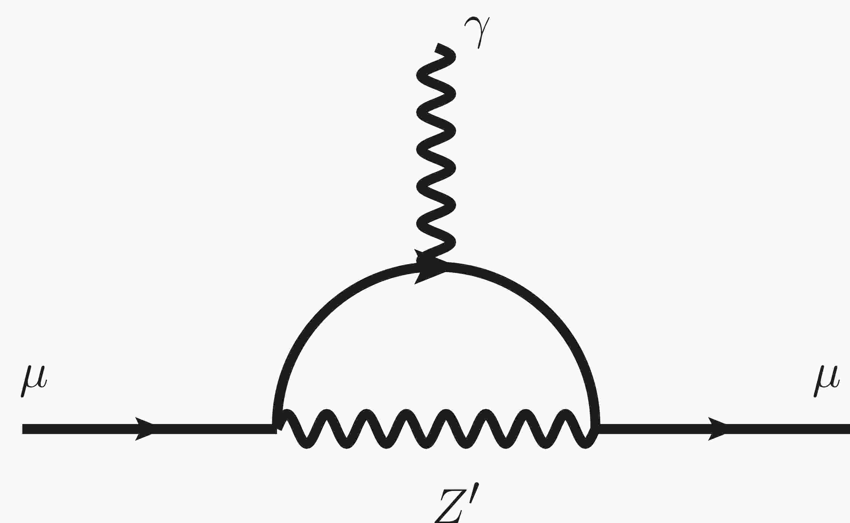
$ (g-2)_{\mu} $ constraints on the$ M_{Z_p}-g_p $ plane, as one goal for introducing$ U(1)_{L _{\mu}- L_{\tau}} $ symmetry is to explain the$ (g-2)_{\mu} $ anomaly. The contribution of the new gauge boson$ Z' $ to the muon anomalous magnetic momentum is shown in Fig. 1. The analytical expression for$ \Delta a_\mu $ is [54]
Figure 1. One-loop contribution of
$ Z' $ to$ (g-2)_{\mu} $ anomaly.$ \Delta a_\mu = \frac{g_p^2 m_{\mu}^2}{8\pi^2} \int_{0}^{1} \frac{2x^2(1-x)}{x^2 m_{\mu}^2+(1-x)M_{Z_{p}}^2} {\rm d}x , $

(21) where
$ m_{\mu} $ is the muon mass.Experimental searches for new gauge bosons have already provided the most stringent constraint on the parameter space of
$ M_{Z_p}-g_p $ . At colliders, the$ Z' $ gauge boson can be produced via$ e^+ e^- \to \mu^+ \mu^- Z' $ with the subsequent decay of$ Z'\to\mu\mu $ . Such a search can be found in Babar [29] and provides a possible bound on the$ M_{Z_p}-g_p $ plane. Additionally, neutrino experiments provide new clues for constraining the parameter space. The Borexino data related to the scattering of low energy solar neutrinos [55, 56] can provide the most stringent constraint on the low$ M_{Z_p} $ and low$ g_p $ region. Another constraint is from the CCFR collaboration [57], obtained via the neutrino trident production, which is related to the process$ \nu N \to \nu N \mu^+ \mu^- $ , where a muon neutrino scatters off of a nucleus, producing a$ \mu^+ \mu^- $ pair. This process will be enhanced by the existence of$ Z' $ compared with the SM case, which gives strong bounds on the possible$ Z' $ contribution and constrains the$ M_{Z_p}-g_p $ parameter space accordingly. In our study, we focus on the low$ M_{Z_p} $ region. The combined experiments as well as$ (g-2)_{\mu} $ constraints on the$ M_{Z_p}-g_p $ are illustrated in Fig. 2. According to Fig. 2, CCFR gives the most stringent constraint on the parameter space of interest in the low$ M_{Z_p} $ region. The Borexino limits become relevant at smaller$ M_{Z_p} $ and$ g_p $ . For$ M_{Z_p} \subseteq [0.2,5] $ GeV, BABAR data plays an important role in constraining$ M_{Z_p} $ and$ g_p $ .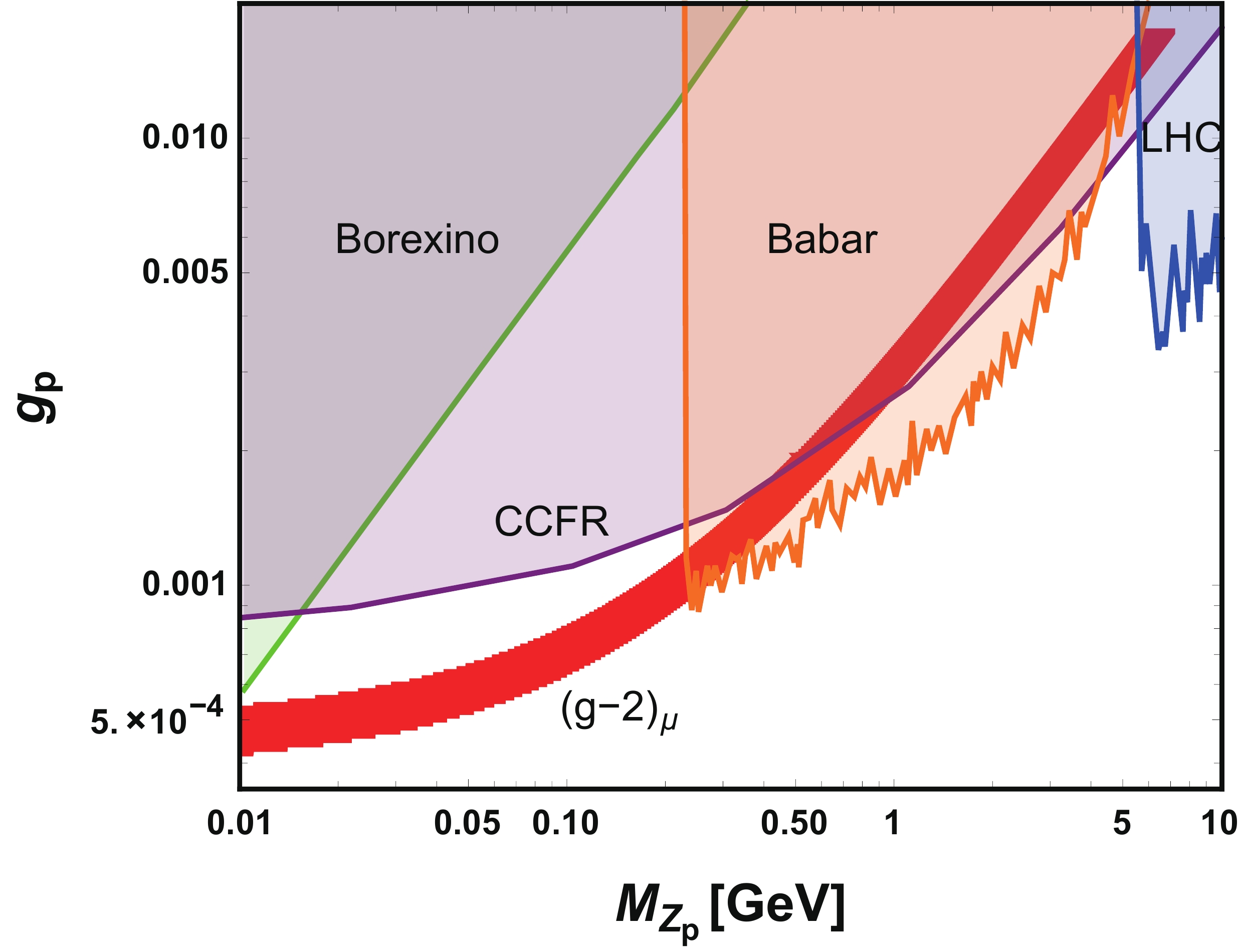
Figure 2. (color online) Allowed region that can explain the
$ (g-2)_{\mu} $ anomaly and the excluded region on$ M_{Z_p}-g_p $ from various experiments: the green (orange, blue, purple) region is excluded by Borexino (BABAR, LHC, CCFC). The red region is the parameter space satisfying the$ (g-2)_{\mu} $ anomaly.We focus on the constraints on
$ M_{Z_p}-g_p $ from experimental data, and it is worth emphasizing that for$ M_{Z_p} \sim 10-20 $ MeV and$ g_p \sim (3-8) \times 10^{-4} $ satisfying the$ (g-2)_{\mu} $ anomaly, the decays of$ Z' $ can heat the neutrino population and delay the process of neutrino decoupling, resulting in$ \Delta N_{\rm eff} \sim 0.2-0.5 $ , according to [58], where$ \Delta N_{\rm eff} $ is the difference from the effective number of neutrino spceies$ N_{\rm eff} $ [59].To sum up, most of the parameter space to explain
$ (g-2)_{\mu} $ has been excluded by these experiments, except for$ M_{Z_p} \subseteq [0.01,0.25] $ GeV and$ g_p $ at the$ 10^{-3} $ level. -
In our model, we have a new gauge boson
$ Z' $ and two scalar fields$ S_{ \rm I} $ and$ S_{ \rm R} $ , We assume that all of these particles masses are smaller than the SM Higgs mass with$ M_{Z_p} <1/2 m_1 $ ,$ m_{\rm I}< 1/2 m_1 $ , and$ m_{\rm R}< 1/2 m_1 $ so that the SM Higgs can decay to these particles, which will contribute to the invisible Higgs decay width. The current constraint on this invisible branching fraction is$ {\rm Br}(h \to {\rm i}nv) <0.24 $ according to the observations at the LHC for the SM Higgs [60], which means$ \frac{\Gamma(h \to {\rm i}nv)}{\Gamma(h \to {\rm i}nv)+\Gamma(h \to {\rm SM})} <0.24 . $

(22) The decay widths related to the Higgs invisible decay channel in our model are given as follows:
$ \begin{aligned}[b] \Gamma_{h_1 \to S_{ \rm I} S_{ \rm I}} =& \sqrt{m_1^2 (m_1^2-4 m_{\rm I}^2)}/(8 \pi m_1 ^3) \\ &\times (\cos\theta\lambda_{Hs}v+\lambda_{ds} \sin\theta v_b -\lambda_{S P} \sin\theta v_b)^2,\\ \Gamma_{h_1 \to S_{ \rm R} S_{ \rm R}} =& \sqrt{m_1^2 (m_1^2-4 m_{\rm R}^2)}/(8 \pi m_1 ^3) \\ &\times (\cos\theta\lambda_{Hs}v-\lambda_{ds} \sin\theta v_b -\lambda_{S P} \sin\theta v_b)^2,\\ \Gamma_{h_1 \to Z' Z'} =& g_p^4\sqrt{m_1^2 (m_1^2-4 M_{Z_p}^2)} /(2 M_{Z_p}^4 \pi m_1 ^3) \\ &\times (m_1^4-4m_1^2M_{Z_p}^2+ 12M_{Z_p}^4) \sin^2\theta v_b^2 . \end{aligned}$

(23) In this section, we consider the Higgs invisible decay constraint on the chosen parameter space. As will be clear in the following discussion,
$ \lambda_{ds} $ is limited stringently under the relic density constraint, while$ \lambda_{Hs} $ and$ \lambda_{S P} $ are more flexible. According to Eq. (22), the contribution of$ \lambda_{Hs} $ to the Higgs invisible decay width is positive, while$ \lambda_{S P} $ is negative. For simplicity, we can set$ \lambda_{Hs} $ and$ \lambda_{S P} $ to be some special values and give the result of the Higgs invisible decay width of our model to estimate the chosen parameter space. In Fig. 3, we set$ \lambda_{Hs}=0.005 $ ,$ \lambda_{S P}=0.001 $ ,$ M_{Z_p}=0.2\ {\rm{GeV}} $ ,$ g_p=0.001 $ ,$ \rm sin\theta=0.001 $ , and$ m_2= 600\ {\rm{GeV}}. $ We also set$ \lambda_{ds} \subseteq [1 \times 10^{-5},0.01] $ and$ m_0 \subseteq [0, 60] \; {\rm{GeV}}. $ According to Fig. 3, the Higgs invisible decay width is much lower than the current constraint in the case of$ \lambda_{Hs}=0.005 $ and$ \lambda_{S P}=0.001 $ . As discussed above, we can set$ \lambda_{Hs}<0.005 $ and$ \lambda_{S P}>0.001 $ to obtain a viable parameter space satisfying the Higgs invisible decay width constraint. It is worth emphasizing that the Higgs invisible decay width is also related to$ \rm sin\theta $ , and in particular, we have a${ \rm \lambda}_{ds}{\rm sin}\theta $ term; when$ \rm sin\theta $ takes a small value,$ \lambda_{ds} $ has little effect on the Higgs invisible decay width.
Figure 3. (color online) Contourplot of Higgs invisible decay width, where the X-axis is
$ m_0 $ and Y-axis is$ \lambda_{ds} $ when$ \lambda_{Hs}= $ $ 0.005 $ ,$ \lambda_{S P}=0.001 $ ,$M_{Z_p}=0.2\ {\rm GeV}$ ,$ g_p=0.001 $ ,$ \rm sin\theta=0.001 $ , and$ m_2= 600\ {\rm{GeV}} $ . -
In this section, we discuss the dark matter phenomenology in the model. The expression for the relic abundance of dark matter can be given as follows:
$ \Omega h^2 = \frac{1.07\times 10^9 \;{{\rm{GeV}}}^{-1} }{{g*}^{1/2}M_{\rm Pl}}\frac{1}{J(x_f)}, $

(24) where
$ g* $ is the total number of effective relativistic degrees of freedom,$ M_{\rm Pl}=1.22\times 10^{19} $ GeV is the Planck mass, and$ J(x_f) $ is given by:$ J(x_f)=\int _{x_f}^\infty \frac{{\rm d}x}{x^2} \langle \sigma {\rm v} \rangle (x) . $

(25) The freeze-out parameter
$ x_f $ in the integral is [61]:$ x_f =\ln \frac{0.038 g M_{\rm Pl} m_{\rm DM} \langle \sigma {\rm v} \rangle (x_f)}{( {g*} x_f )^{1/2}}, $

(26) where
$ m_{\rm DM} $ is the dark matter mass, g is the dark matter's effective number of degrees of freedom, and$ \langle \sigma{\rm v} \rangle (x) $ is the thermally averaged product of the effective dark matter annihilation cross-section and the relative speed of the dark matter pair in their center-of-mass frame. According to the current experiment, the dark matter relic density is [62]:$ \Omega h^2 =0.1198 \pm 0.0012 . $

(27) Scalar dark matter in our model is stabilized by
$ Z_2 $ symmetry after$ U(1)_{L_{\mu}-L_{\tau}} $ spontaneously breaks symmetry. It is worth noting that another scalar$ S_{ \rm R} $ can also play the role of dark matter when$ S_{ \rm I} $ and$ S_{ \rm R} $ are nearly degenerate. The dark matter relic density will be determined not only by$ S_{ \rm I} $ , but also by$ S_{ \rm R} $ , which is the so-called co-annihilation case [63]. In the case we considered, the number density of$ S_{ \rm R} $ will track the$ S_{ \rm I} $ number density during freeze-out, when the relative mass splitting Δ is small compared with the freeze-out temperature, which is defined by:$ \Delta \equiv \frac{m_{\rm R}-m_{\rm I}}{m_{\rm I}} . $

(28) Concretely speaking, the relic density is calculated by solving the Boltzman equation, which depends on the dimensionless variable
$ x=m_{\rm DM}/T $ . Freeze-out occurs at$ x_{\rm F}=m_{\rm DM}/T_{\rm F} \approx 20\sim 30 $ for cold, non-relativistic dark matter, where$ T_{\rm F} $ is the freeze-out temperature. For$ \delta m = m_{\rm R}-m_{\rm I} $ much larger than$ T_{\rm F} $ , we simply have dark matter$ S_{ \rm I} $ annihilations freeze-out. However,$ S_{ \rm R} $ will be thermally accessible when$ \delta m \approx T_{\rm F} $ . Hence, the relative mass splitting Δ can give the upper bound of$ \Delta \sim x_{\rm F}^{-1} \sim 0.03-0.05 $ when we consider the co-annihilation case. A more systematic estimate for the contribution of Δ to relic density can be found in [36, 64], and a necessary mass splitting for successful co-annihilation is typically$ \Delta \leqslant 0.3 $ , according to [64]. Δ in our model can be written as follows:$ \Delta = \frac{m^2_{\rm R}-m^2_{\rm I}}{m_{\rm I}(m_{\rm I}+m_{\rm R})}=\frac{2\lambda_{ds}v^2_b}{m^2_{\rm I}+m_{\rm I}m_{\rm R}} . $

(29) According to Eq. (29), co-annihilation becomes more significant in the model as long as
$ \lambda_{ds}v_b^2 \ll m_{\rm I}^2 $ , where$ S_{ \rm I} $ and$ S_{ \rm R} $ are kept in equilibrium via the interactions$ S_{ \rm I} S_{ \rm I} \leftrightarrow S_{ \rm R} S_{ \rm R} $ , while in the light dark matter case, the main contribution of relic density arises from the annihilation of$ S_{ \rm I} $ . Before we consider the relic density numerically, we should stress that the co-annihilation process can be dominated during the evolution of relic density in the heavy dark matter case, but we want to consider a viable region where annihilation and co-annihilation can be both involved, which means that the dark matter mass we considered should not be too heavy. We choose a viable parameter space with$ 0\leqslant m_0\leqslant 60 $ GeV, and the dark matter particle mass will be constrained to range from a few GeV to approximately 70 GeV. Annihilation and co-annihilation processes will be both involved within the chosen parameter space, as will be clear in the following discussion.The Feynman diagrams relevant for the production of dark matter are given in Fig. 4. According to Fig. 4, scalar dark matter can annihilate into SM particles with Higgs-mediated interactions. In the case of
$ 2m_{\rm DM}>M_{Z_p} $ as we have assumed, dark matter can annihilate into a pair of$ Z' $ via the t-channel, as shown in Fig. 4(e). In particular, in the case of the light dark matter region where$ S_{\rm I} $ and$ S_{ \rm R} $ cannot be degenerate, we have a t-channel process with$ S_{{\rm R}\mu} \rightarrow S_{{\rm I} \mu} $ as in Fig. 4 (g), which can also contribute to the relic density. Vertices related to these Feynman diagrams are given in Table 1 for$ S_{\rm I} $ annihilation. As discussed above,$ S_{\rm R} $ can also play the role of dark matter in the case of co-annihilation, and the relevant vertices are also given in Table 1.Coupling Vertex factor ${\cal C}_{S_{\rm {I(R)} } S_{{\rm {I(R)}} h_1} }$ 

$-{\rm i} [2 v \lambda_{Hs} \cos\theta \pm 4 v_b \lambda_{ds}\sin\theta \mp 2 v_b \lambda_{S P} \sin\theta]$ 

$ {\cal C}_{S_{\rm {I(R)}} S_{\rm {I(R)}} h_2} $ 

$ -{\rm i} [2 v \lambda_{Hs} \sin\theta \mp 4 v_b \lambda_{ds}\cos\theta \pm 2 v_b \lambda_{S P} \cos\theta] $ 

$ {\cal C}_{S_{\rm {I(R)}} S_{\rm {I(R)}} h_1 h_1} $ 

$ -{\rm i}[2 \lambda_{Hs} \cos^2\theta \mp 4 \lambda_{ds}\sin^2\theta + 2 \lambda_{S P} \sin^2\theta] $ 

$ {\cal C}_{S_{\rm {I(R)}} S_{\rm {I(R)}} h_2 h_2} $ 

$-{\rm i} [2 \lambda_{S P} \cos^2\theta \mp 4 \lambda_{ds}\cos^2\theta + 2 \lambda_{Hs} \sin^2\theta]$ 

$ {\cal C}_{S_{\rm {I(R)}} S_{\rm {I(R)}} h_1 h_2} $ 

$ -{\rm i} \cos\theta \sin\theta [2 \lambda_{Hs} \pm 4 \lambda_{ds} - 2\lambda_{S P}] $ 

${\cal C}_{S_{\rm I} S_{\rm R} Z'}$ 

$\dfrac{2}{3}g_p(p_1-p_2)^{\mu}$ 

${\cal C}_{S_{\rm {I(R)}} S_{\rm {I(R)}} Z'Z'}$ 

${\rm i} 16 g_p^2$ 

Table 1. Vertices related to
$ S_{\rm {I(R)}} $ annihilation.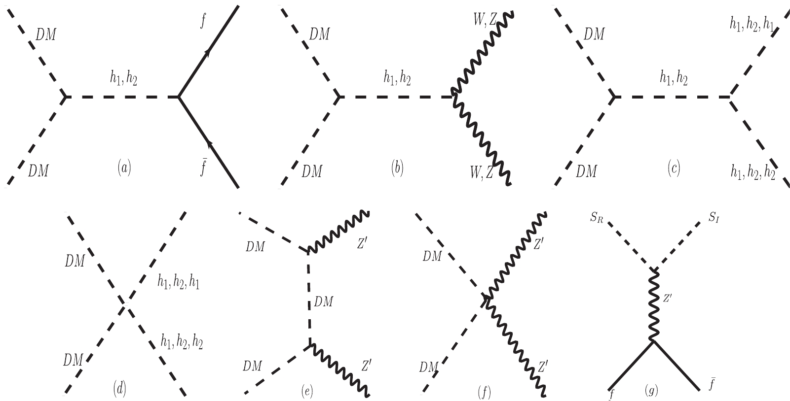
Figure 4. Feynman diagrams related to dark matter relic density.
In this work, we use Feynrules [65] to generate the implemented code, micrOmegas [66] to calculate the relic density, and t3ps [67] to scan the parameter space. For simplicity, we assume
$ \lambda_s=0 $ because the self interaction part of dark matter makes no contribution to the relic density. Moreover, searches for the exotic Higgs at the LHC give upper limits of the mixing angle of$ |\sin\theta| \leqslant 0.2 \sim 0.6 $ , depending on the heavy Higgs mass [68–71]. In addition, as we discussed above,$ M_{Z_p} $ and$ g_p $ are limited in the current experiments. To summarize, there are 8 independent parameters in the model, and we use three scenarios to estimate these parameters separately for simplicity. In$ Scenario\ A $ , we consider the$ (g-2)_{\mu} $ anomaly as well as dark matter relic density constraint on$ M_{Z_p}-g_p $ . In$ Scenario\ B $ , we discuss the contribution of various parameters to the dark matter relic density. In$ Scenario\ C $ , we focus on the relic density constraint on the couplings$ \lambda_{Hs} $ ,$ \lambda_{S P} $ , and$ \lambda_{ds} $ . -
In this section, we focus on the
$ (g-2)_{\mu} $ anomaly as well as the dark matter relic density constraint on$ M_{Z_p}-g_p $ , where the inputs are given in Table 2. According to Fig. 5, the allowed region to satisfy the relic density constraint (blue dots) and the$ (g-2)_{\mu} $ anomaly (red region) is$ M_{Z_p}\subseteq [0.01,0.25] $ GeV and$ g_p \subseteq [4 \times 10^{-4},0.002] $ where we have set$ \sin\theta = 0.01 $ ,$ m_2 \subseteq [0.2,2] $ TeV, and$ \lambda_{Hs, S P, ds} \subseteq [10^{-5},0.1] . $ Because we have chosen$ m_2 $ and$ v_b=M_{Z_p}/2g_p $ as inputs, these parameters should be limited by perturbative constraint as well as vacuum stability constraint, which means that$ v_b=M_{Z_p}/2g_p $ should not be too small. We focus on the light scalar$ S_{\rm R} $ mass at a few GeV, where contribution to the$ N_{\rm eff} $ can be negligible. As we can see from Fig. 5, most of the blue points fall in the lower-right region, and the upper-left region is excluded within the chosen parameter space.Parameter Value for inputs $m_2/{\rm TeV}$ 

$ [0.2,2] $ 

$ \sin \theta $ 

0.001 $\lambda_{H s}$ 

$ [10^{-5},0.1] $ 

$\lambda_{S P}$ 

$ [10^{-5},0.1] $ 

$ \lambda_{ds} $ 

$ [10^{-5},0.1] $ 

$M_{Z_p}/{\rm GeV}$ 

$ [0.01,0.25] $ 

$ g_p $ 

$ [4 \times 10^{-4},0.002] $ 

$m_0 /{\rm GeV}$ 

$[0, 60]$ 

Table 2. Values for parameters as input to calculate dark matter relic density.
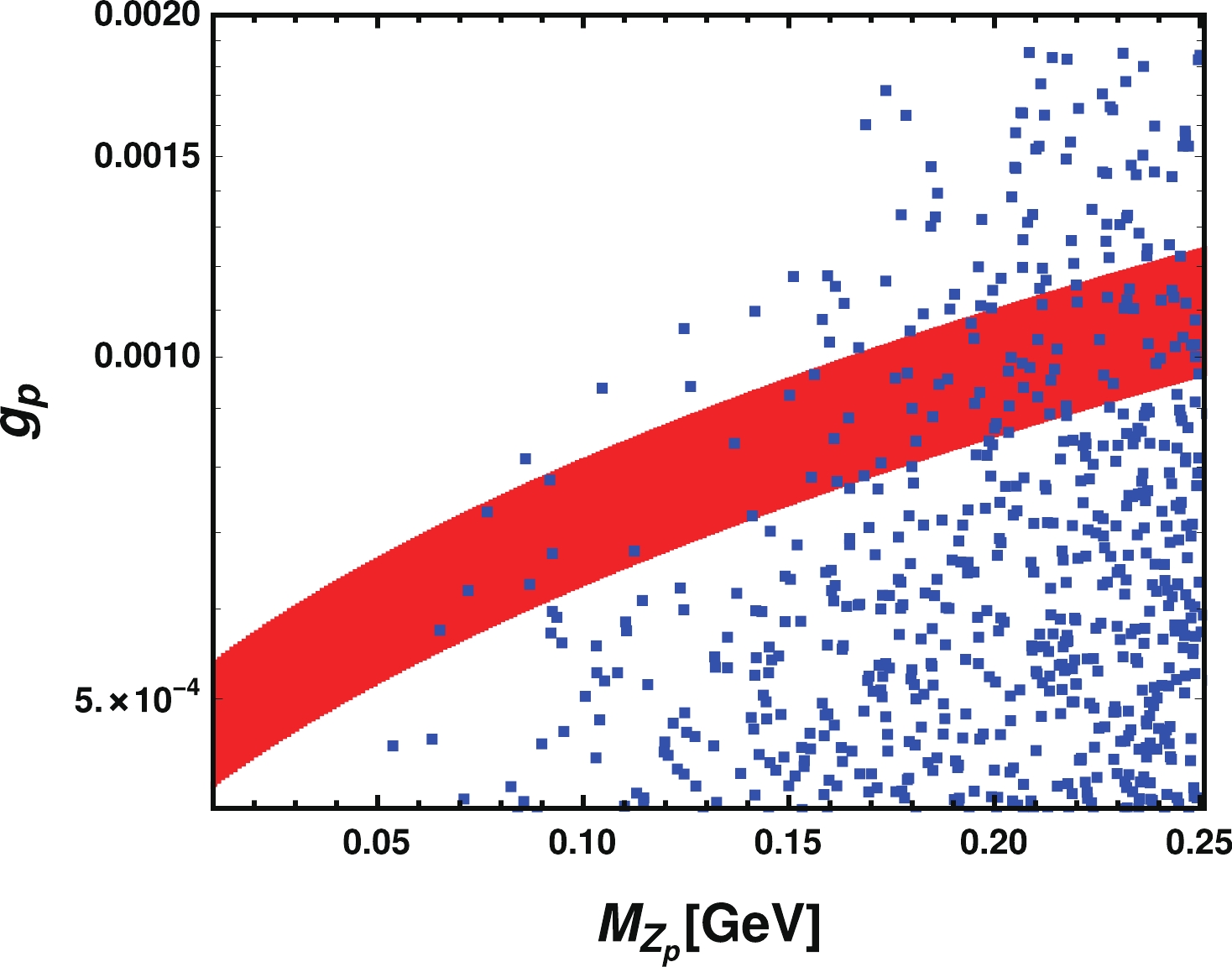
Figure 5. (color online) Allowed
$ M_{Z_p}-g_p $ region to satisfy relic density constriant (blue dots) and$ (g-2)_{\mu} $ anomaly [red region] with$ M_{Z_p}\subseteq [0.01,0.25] $ GeV and$ g_p \subseteq [4 \times 10^{-4}, 0.002] $ , where we have set$ \sin\theta=0.01 $ ,$ m_2\subseteq [0.2,2] $ TeV, and$\lambda_{Hs, S P, ds} \subseteq $ $ [10^{-5},0.1]$ ,$ m_0\subseteq [0, 60] $ GeV. -
In this section, we discuss the contribution of other parameters to the dark matter relic density. The results of relic density are shown in Fig. 6, where curves with different colors correspond to one of the parameters. We set
$ 0 \leq m_0 \leq 60\;{\rm{GeV}} $ , and the benchmark values for the parameters are given in Table 3. We fix$ M_{Z_p}=0.2 $ GeV and$ g_p=0.001 $ in Fig. 6 (top), while in Fig. 6 (bottom), we fix$ M_{Z_p}=0.1 $ GeV and$ g_p=0.0007 $ .
Figure 6. (color online) Value of relic density as a function of
$ m_0 $ . The purple solid curve is the experimentally observed relic density [62]. Curves with different colors correspond to different parameters when$ M_{Z_p}=0.2 $ GeV,$ g_p=0.001 $ (top figure) and$ M_{Z_p}=0.1 $ GeV,$ g_p=0.0007 $ (bottom figure).Parameter Benchmark value for input $ m_2/{\rm GeV} $ 

300 $ \sin\theta $ 

0.001 $\lambda_{H s}$ 

$ 1 \times 10^{-4} $ 

$\lambda_{S P}$ 

$ 1 \times 10^{-4} $ 

$ \lambda_{ds} $ 

$ 1 \times 10^{-4} $ 

$ M_{Z_p}/{\rm GeV} $ 

0.2 $ g_p $ 

0.001 Table 3. Benchmark values for parameters as input to calculate dark matter relic density.
In Fig. 6 (top), the purple solid curve is the experimentally observed relic density. Curves corresponding to
$ m_2=600 $ GeV and$ \sin\theta=0.03 $ almost coincide with the benchmark curve, which occurs because dark matter annihilation channels related to Higgs make little contribution to relic density in these cases. Correspondingly, for the red line with$\lambda_{H s}=0.01$ , there is a resonance region at approximately$ 2m_{\rm DM}=m_1 $ , where the relic density decreases sharply and intersects with the relic density constraint curve. For$ \lambda_{ds}=0.001 $ , i.e., the blue dashed curve, the dark matter mass can be negative when$ m_0 $ has a small value, so that the starting point of the curve is not$ m_0=0 $ . For Fig. 6 (bottom), with$ M_{Z_p}=0.1 $ GeV and$ g_p=0.0007 $ , the curves are almost the same with those in Fig. 6 (top), and one of the typical differences is that the blue dashed curve corresponding to$ \lambda_{ds}=0.001 $ starts at$ m_0=0 $ and intersects with the relic density constraint curve. According to these figures, we can reduce the inputs to$ \lambda_{ds} $ ,$ \lambda_{S P} $ ,$ \lambda_{Hs} $ ,$ m_0 $ ,$ M_{Z_p} $ , and$ g_p $ , as the contributions of$ m_2 $ and$ \sin\theta $ to relic density are small. -
In this section, we scan the parameter space to study the relic density constraint on the couplings. For simplicity, we fix
$ M_{Z_p} $ ,$ g_p $ ,$ \sin\theta $ , and$ m_2 $ , and focus on$ \lambda_{S P} $ ,$ \lambda_{ds} $ , and$ \lambda_{H s} $ . It is worth emphasizing that$ Z' $ is not stable and can decay into a pair of muon neutrinos as well as tauon neutrinos. We set these parameters as in Table 4. To avoid$ m_{\rm DM} $ having a value that is too large, we have set the couplings$ \lambda_{Hs, S P, ds} $ to be smaller than 0.01. The results are given in Fig. 7. According to the first image in Fig. 7, the possible dark matter$ S_{\rm I} $ mass ranges from a few GeV to approximately$ m_1/2 $ , as discussed above, and for$ m_{\rm I} $ larger than approximately 3.3 GeV, we have$ m_{\rm R} \approx m_{\rm I} $ and the co-annihilation process can dominate the evolution of relic density where both$ S_{\rm R} $ and$ S_{\rm I} $ play the role of dark matter. When$ S_{\rm I} $ takes a smaller value, Δ can be very large, and only$ S_{\rm I} $ plays the role of dark matter. In addition, we give the scan results of$ \lambda_{ds}-m_{\rm I} $ ,$ \lambda_{Hs}-m_{\rm I} $ and$ \lambda_{S P}-m_{\rm I} $ in the other images in Fig. 7 separately. It is clear from the second image that the allowed value of$ \lambda_{ds} $ is constrained within a narrow region when$ m_{\rm I} $ is in the region of$ [3.3,\; 50\ {\rm{GeV}}] $ and increases as$ m_{\rm I} $ increases; this result is seemingly contrary to Eq. (9), where$ m_{\rm I} $ decreases as$ \lambda_{ds} $ increases. This means that$ \lambda_{H s} $ and$ \lambda_{S P} $ play a more important role in determining dark matter mass under the relic density constraint. For$ m_{\rm I} \leqslant 3.3\ {\rm{GeV}} $ ,$ \lambda_{ds} $ is constrained in$ [0.001,0.01] $ and decreases when$ m_{\rm I} $ increases, following Eq. (9). For$ m_I>50 $ GeV,$ \lambda_{ds} $ can take a value within the whole range of$ [1\times 10^{-5}, 0.0084] $ . In the last two images, both$ \lambda_{H s} $ and$ \lambda_{S P} $ can take values from$ 1 \times 10^{-5} $ to$ 0.01 $ , and a certain number of points fall in the region$ [0,001, 0.01] $ , with a few points obtained in the low mass region.Parameter Value for inputs $ m_2/{\rm GeV} $ 

300 $ \sin \theta $ 

0.001 $ M_{Z_p}/{\rm GeV} $ 

0.2 $ g_p $ 

0.001 $ m_0/{\rm GeV} $ 

$ [0, 60] $ 

$\lambda_{H s}$ 

$ [10^{-5},0.01] $ 

$\lambda_{S P}$ 

$ [10^{-5},0.01] $ 

$ \lambda_{ds} $ 

$ [10^{-5},0.01] $ 

Table 4. Values for parameters as input for scan.
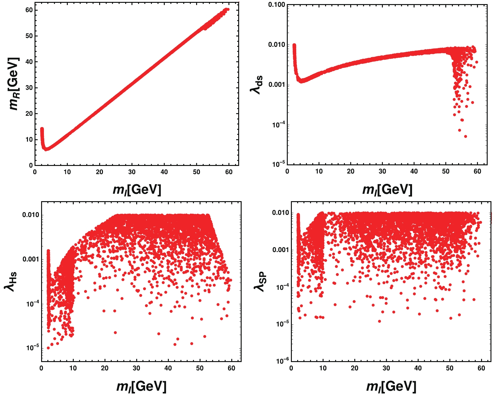
Figure 7. (color online) Scatter points satisfying relic density constraint, with the X-axis being
$ S_{\rm I} $ mass and Y-axis being$ S_{\rm R} $ mass in the first image. The scan results of$ \lambda_{ds}-m_{\rm I} $ ,$ \lambda_{Hs}-m_{\rm I} $ , and$ \lambda_{S P}-m_{\rm I} $ are given in the second, third, and fourth images, respectively. -
Experiments related to dark matter direct detection such as CDMS II [72], XENON100 [73], XENON1T [74], and LUX [75] have been searching for signals related to the interaction of dark matter with nucleons. In our model, we have two constraints arising from tree level and loop level explicitly. On the one hand, quarks do not couple with
$ Z' $ , but only with two Higgs particles, and these interactions can be concluded by the scattering of dark matter particles off a SM fermion f via the t-channel exchange of the two Higgs particles, which is similar to the two singlet scalar model [76, 77]. The effective Lagrangian for dark matter-quark elastic scattering can be given by$ {\cal L}_{q,{\rm eff}}=-\frac{m_q}{2v}\left(\frac{{\cal C}_{h_1S S}\cos\theta}{m_1^2} + \frac{{\cal C}_{h_2S S}\sin\theta}{m_2^2}\right)S S \bar{q}q , $

(30) and the effective Lagrangian related to
$ S_{\rm I }$ and$ S_{\rm R} $ can be given by$ {\cal L}_{q,{\rm eff}}=\sum_{S=S_{\rm R},S_{\rm I}} -\frac{m_q}{2v}\left(\frac{{\cal C}_{h_1S S}\cos\theta}{m_1^2} + \frac{{\cal C}_{h_2S S}\sin\theta}{m_2^2}\right)S S \bar{q}q .\; $

(31) Furthermore, the effective Lagrangian related to dark matter-nucleon elastic scattering can be given by:
$\begin{aligned}[b] {\cal L}_{N,{\rm eff}} =& \sum_{S=S_{\rm R},S_{\rm I}} \frac{m_N-\dfrac{7}{9}m_B}{v} \\ &\times \left(\frac{{\cal C}_{h_1S S}\cos\theta}{m_1^2}+ \frac{{\cal C}_{h_2S S}\sin\theta}{m_2^2}\right)S S \bar{N}N, \end{aligned}$

(32) where
$ m_N $ represents the nucleon mass and$ m_B $ represents the baryon mass in the chiral limit [43]. The total cross section for$ S-N $ elastic scattering can be given by$ \sigma_{SN\rightarrow SN} =\frac{m^4_Nf_N^2}{4\pi (m_N+m_{\rm DM})^2} \times \left(\frac{{\cal C}_{h_1S S}\cos\theta}{m_1^2}+ \frac{{\cal C}_{h_2S S}\sin\theta}{m_2^2}\right)^2, $

(33) where
$ f_N $ is the Higgs-nucleon Formfactor with$ f_N= 0.308(18) $ , according to the phenomenological and lattice-QCD calculations [78], and$ m_{\rm DM} $ corresponds to both$ m_{\rm I} $ and$ m_{\rm R} $ .On the other hand, dark matter particles can scatter off nuclei through a loop of charged leptons coupling to photons, which couple to protons as in Fig. 8. The first diagram in Fig. 8 is the most relevant, and the rest two are 2-loop suppressed and negligible. In our model, we have the
$S_{{\rm R} N} \rightarrow S_{{\rm I} N}$ process, and a similar process can be found in [38], where the dark matter candidate is a fermion. In particular, we have a similar WIMP-nucleon scattering cross section [79] in the case of$S_{\rm R} \approx S_{\rm I}$ :
Figure 8. Feynman diagrams related to spin-independent dark matter-nucleon scattering at the one loop level.
$ \sigma =\frac{1}{A^2}\frac{\mu_N^2}{9\pi}\left(\frac{2\alpha_{\rm em}Zg_p^2}{\pi M_{Z_p}^2}\log\left(\frac{m^2_{\mu}}{m^2_{\tau}}\right)\right)^2 . $

(34) Because the theoretical results are compared with current limits from Xe-based experiments, we set
$ \mu_{N}=m_{\rm Xe}m_{\rm DM}/ (m_{\rm Xe}+m_{\rm DM}) $ , which is the WIMP-nucleus reduced mass, where$ m_{\rm Xe} $ is the Xe nucleus mass and$ m_{\rm Xe} \approx129 $ GeV. Correspondingly, Z is the atomic number of Xe, with$ Z=54 $ , and A is the mass number of Xe.As discussed above, we have two cases, corresponding to tree level and loop level in direct detection, and the tree level contribution is much smaller than the loop level, even though our model is loop-suppressed. This result can be understood by considering that the cross section of the loop contribution is proportional to the nucleus electric charge, while the tree level is strictly suppressed by the Higgs mass.
We consider the direct detection constraint on the chosen parameter space of the model, and the result is given in Fig. 9, where the plot is drawn as a function of
$ m_{\rm I} $ . The red points represent the result of the chosen parameter space satisfying the relic density constraint, the blue curve represents the result of XENON1T [80], the black curve represents the result from the light dark matter search in XENON1T [81], the orange curve represents results from Darkside-50 [82], and the green curve represents the constraint from CRESST-III [83] in the light dark matter region. According to Fig. 9, direct detection gives the most stringent limit on the parameter space, and most of the region above 5 GeV is excluded by XENON1T [80]. In addition, XEN0N1T [81] excludes the region above 3.7 GeV in the light dark matter region. However, the range of$ [3.3,\; 3.7\ {\rm{GeV}}] $ is not excluded, which satisfies the co-annihilation condition. Most importantly, in our model, a region of a few GeV is still allowed, in spite of the severe constraint from direct detection, and the co-annihilation process is also permitted in our model, as discussed above.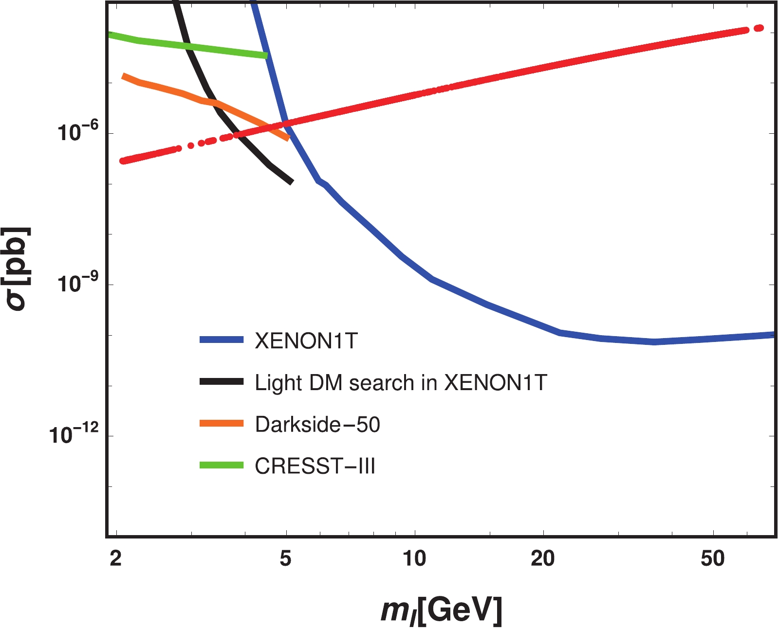
Figure 9. (color online) Spin independent cross section as a function of
$ m_{\rm I} $ ; the red points represent the result of the chosen parameter space satisfying the relic density constraint, the blue curve represents the result of XENON1T [80], the black curve represents the result from the light dark matter search in XENON1T [81],the orange curve represents results from Darkside-50 [82], and the green curve represents the result of the CRESST-III experiment [83]. -
The SM has achieved great success because of its high accuracy in describing electroweak and strong interactions. However, there remain problems, such as the neutrino mass and dark matter, that the SM cannot explain. In addition, recent results regarding the muon anomalous magnetic moment
$ (g-2)_\mu $ offer new challenges to the SM. The$ 4.2\sigma $ discrepancy between experiment and SM prediction seems to indicate new physics behind the$ (g-2)_{\mu} $ anomaly and gives possible hints to what is beyond the SM. Among these models, a gauged$ U(1)_{L_{\mu}-L{\tau}} $ model stands out because of its simplicity, as the gauge anomaly cancellation can be accomplished without introducing extra fermions. Related discussions regarding this model and experiments constrain the new gauge boson$ Z' $ mass at the MeV scale, which are also satisfied with the$ (g-2)_{\mu} $ constraint. In addition, one can also introduce new particles to the$ {L_{\mu}-L_{\tau}} $ model so that the dark matter problem as well as the neutrino mass problem can be explained.In this article, we consider a scalar dark matter model within the frame of a gauged
$ {L_{\mu}-L_{\tau}} $ model. We introduce a new gauge boson$ Z' $ as well as two scalar fields S and Φ to the SM. The lighter component of S can play the role of dark matter, which is stabilized by an extra$ Z_2 $ symmetry after spontaneously breaking symmetry. In this work, we focus on dark matter and the$ (g-2)_{\mu} $ anomaly and ignore the neutrino mass problem. In the case of$ m_{\rm I} <m_1/2 $ ,$ m_{\rm R} <m_1/2 $ , and$ M_{Z_p} <m_1/2 $ , we have new Higgs invisible channels, which should be limited by the current experimental result at the LHC. We consider the possibility of light dark matter as well as the co-annihilation case in our model. We discuss relic density constraint and find that in the case of$ m_{\rm I} $ on the order of a few GeV, the imaginary part$ S_{\rm I} $ of S can be considered light dark matter with$ m_{\rm R} $ much larger than$ m_{\rm I} $ . However, with$ m_{\rm I} $ increasing, the allowed values for$ m_{\rm I} $ and$ m_{\rm R} $ are approximately equal, so that we have$ \Delta \approx 0 $ , and we come to the so-called co-annihilation process, where both$ S_{\rm R} $ and$ S_{\rm I} $ play the role of dark matter. For$ m_{\rm I} < 50 $ GeV, the relic density constraint limits$ \lambda_{ds} $ stringently, which plays a significant role in determining$ m_{\rm I} $ and$ m_{\rm R} $ . We have two cases, arising from the tree level and loop level, when discussing the direct detection constraint on our model, and the tree level contribution is much smaller than that of the loop level, even though our model is loop-suppressed. Direct detection gives the most stringent limit on the parameter space, and most of the region above 3.7 GeV is excluded. In our model, a region of a few GeV is still allowed in spite of the severe constraint from direct detection, and the co-annihilation process is also permitted in our model. According to [84], one can consider the generation of$ Z' $ via$ Zh_1 $ associated production, followed by$ h_1 $ decaying into a$ Z' $ pair process in future high energy$ e^+e^- $ colliders, where$ h_1 $ a is the SM-like Higgs boson, and one can conclude that signal significance above$ 5\sigma $ for$ Z' $ detection can be achieved via both these processes with appropriate parameter values and high integrated luminosity. Such a scenario makes it possible to test the model in future experiments.
Scalar dark matter and muon g-2 in a ${\boldsymbol U({\bf 1})_{{\boldsymbol L}_{\boldsymbol\mu} - {\boldsymbol L}_{\boldsymbol\tau}}} $ model
- Received Date: 2022-02-11
- Available Online: 2022-08-15
Abstract: We consider a simple scalar dark matter model within the frame of gauged


 DownLoad: