


 Abstract
 HTML
HTML Reference
 Related
 PDF
PDF


-
One of the most important events of the 2010s was the direct detection of gravitational waves (GWs), which succeeded in verifying the existence of black holes (BHs) [1, 2]. The BH perturbation theory can describe GWs emitted at the ringdown phase of a coalescence, which are characterized as quasinormal modes (QNMs). The gravitational perturbations of a BH can reflect the nature of the BH itself, and the ringdown phase of GWs is very important for astronomical observations related to compact celestial bodies. Shortly after the first detection of GWs, GWs emitted by the coalescence of two neutron stars were detected by the Ligo-Virgo collaboration [3]. In the meantime, the source emitted accompanying electromagnetic (EM) signals. This exceptional scientific achievement inaugurated a new era of physical observation. Therefore, the ringdown phase of GWs from the coalescence of compact binary celestial bodies (binary BHs, binary neutron stars and BH-neutron stars) plays a very important role in exploring corresponding sources.
Recent observations show the presence of magnetic fields near BHs [4]. In strong magnetic fields, quantum electrodynamics (QED) predicts photon splitting and pair conversion [5]. In fact, because of EM self-interactions in intense EM fields, the vacuum has the nature of a material medium and then the EM wave changes direction (i.e., birefringence [6–8]) and magnitude of velocity. By using the method of waveguides, one is able to detect QED vacuum nonlinearities [9]. Moreover, the method with intense laser pulses has been proposed to detect vacuum polarization effects [10–12].
The Euler-Heisenberg (EH) theory was derived from QED to one loop [13, 14], which treats the vacuum as a medium, and processes of nonlinear light interaction are predicted. In this theory, the EH Lagrangian is
$ \mathcal{L}_{\mathrm{EH}}(F, G)=-\frac{F}{4}+\frac{\mu}{4}\left(F^{2}+\frac{7}{4} G^{2}\right), $

(1) where
$ F=F^{\mu \lambda} F_{\mu \lambda} $ ,$ G=-^{*} F^{\mu \lambda}F_{\mu \lambda} $ .$ F_{\mu \lambda} $ and$ { }^{*} F_{\mu \nu}= \epsilon_{\mu \nu \rho \sigma} F^{\sigma \rho}/2 \sqrt{-g} $ are the electromagnetic tensor and its dual, respectively. In the limit of the weak field, the EH parameter$ \mu=2 \alpha^{2}/45 m_{\rm e}^{4} $ is related to the electron mass$ m_{\rm e} $ and the fine structure constant α [14, 15]. Therefore, the EH parameter μ can be on the order of$ \alpha / E_{\rm c}^{2} $ , where$ E_{\rm c} $ represents the critical electric field. In the limit of$ \mu=0 $ ,$ \mathcal{L}_{\mathrm{EH}}(F, G)=\mathcal{L}_{\rm {Maxwell }}(F)=-F / 4 $ , the EH theory goes back to linear EM Maxwell theory. Coupling the EH theory with Einstein gravity, a static spherically symmetric (SSS) charged solution can be obtained, i.e., the Einstein-Euler-Heisenberg (EEH) BH.It is noteworthy that there has been an increasing interest in using QNMs to test modified gravity theories in recent years [16–28]. In particular, the QNMs in the Einstein-power-Maxwell electrodynamics theory have been investigated, for instance [25, 28]. For the EH theory, Bretón and López have studied the eikonal QNMs of the EEH BH [15]. However, in modified gravity theories, the eikonal approximation may be violated for gravitational perturbations of BHs, such as EiBI charged BHs [29]. In order to determine the potentials in the eikonal limit and further investigate the effects of the EH theory, we will study the QNMs of both the axial and the polar gravitational perturbations. The analysis of the stability of a Schwarzschild singularity ushered the BH perturbation theory [30]. Subsequently, polar gravitational perturbations were studied by Zerilli [31–33]. Chandrasekhar then systematically summarized the BH perturbation theory in his monograph [34]. In fact, a perturbed BH is considered as a dissipative system with a discrete spectrum of complex quasinormal frequencies. In this case, quasinormal frequencies are associated with the spacetime properties of the BH but not the initial disturbances. Thus, the spacetime properties of BHs are accurately reflected by the QNMs. In this paper, the master equations of both the axial and the polar gravitational perturbations are derived. For the accuracy of quasinormal frequencies, the 6th order WKB method is used [35–38], and the quasinormal frequencies are shown to be dependent on the EH parameter μ.
The remainder of this paper is organized as follows. In Sec. II, the formulation of the EH theory and its SSS solution are briefly reviewed. In Sec. III, the master equations governing both the axial and the polar gravitational perturbations of the EEH BH are derived. In Sec. IV, the QNMs and the late-time tails are studied. The conclusion is given in Sec. V.
-
In this section, we rewind briefly to review how to obtain the EEH BH. Nonlinear electrodynamics (NLED) with the Lagrangian
$ \mathcal{L}_{\mathrm{EH}}(F, G) $ are coupled with Einstein gravity as follows:$ S=\frac{1}{4 \pi} \int {\rm d}^{4} x \sqrt{-g}\left[\frac{R}{4}-\mathcal{L}_{\mathrm{EH}}(F, G)\right]. $

(2) There are two possible frameworks for EH-NLED [39]. In the P framework, the tensor
$ P_{\mu \nu} $ is defined by$ P_{\mu \nu}=-\left(\mathcal{L}_{F} F_{\mu \nu}+{ }^{*} F_{\mu \nu} \mathcal{L}_{G}\right), $

(3) where
$ \mathcal{L}_{X}={\rm d} \mathcal{L}_{\mathrm{EH}}(F, G) / {\rm d} X $ . Then$ P_{\mu \nu}=(1-\mu F) F_{\mu \nu}-{ }^{*} F_{\mu \nu} \frac{7 \mu}{4} G. $

(4) In the case of the P framework, there are two invariants s and t,
$ s=-\frac{1}{4} P_{\mu \nu} P^{\mu \nu}, \quad t=-\frac{1}{4} P_{\mu \nu} { }^{*} P^{\mu \nu}, $

(5) where
$ { }^{*} P^{\mu \nu}= \epsilon_{\mu \nu \rho \sigma} P^{\sigma \rho}/2 \sqrt{-g} $ .The Hamiltonian
$ \mathcal{H}(s, t) $ is defined as follows:$ \mathcal{H}(s, t)=-\frac{1}{2} P^{\mu \nu} F_{\mu \nu}-\mathcal{L}_{\mathrm{EH}}(F, G). $

(6) Neglecting the higher order terms of the EH parameter μ, the Hamiltonian
$ \mathcal{H}(s, t) $ takes the form [40]$ \mathcal{H}(s, t)=s-4 \mu\left(s^{2}+\frac{7 \mu}{4} t^{2}\right). $

(7) In the P framework of EH-NLED, the gravitational and EM field equations are
$ G_{\mu \nu}+\Lambda g_{\mu \nu}=8 \pi T_{\mu \nu}, \quad \nabla_{\mu} P^{\mu \nu}=0, $

(8) where
$ \begin{split} T_{\mu \nu}&=\frac{1}{4 \pi}(1-\mu s) P_{\mu}^{\beta} P_{\nu \beta} +\frac{g_{\mu \nu}}{4 \pi}\left(s-\frac{\mu}{2}\left(3 s^{2}+\frac{7}{4} t^{2}\right)\right). \end{split} $

(9) Because the EEH BH, like the Reissner-Nordström (RN) solution, represents an SSS spacetime, we can write the metric as follows:
$ \begin{split} {\rm d} s^{2}&=-f(r) {\rm d} t^{2}+f(r)^{-1} {\rm d} r^{2} +r^{2}\left({\rm d} \theta^{2}+\sin ^{2} \theta {\rm d} \varphi^{2}\right), \end{split} $

(10) where
$ f(r)=1-2 m(r) / r $ was first derived in [41] and then studied in [15, 42]. We would like to emphasize that Eq. (10) represents an electric (or magnetic) charged BH. For simplicity, we have only studied the electric case. In the P framework, the antisymmetric tensor$ P_{\mu \nu} $ is given by$ P_{\mu \nu}=\frac{Q_{\rm e}}{r^{2}}\left(\delta_{\mu}^{1} \delta_{\nu}^{0}-\delta_{\mu}^{0} \delta_{\nu}^{1}\right), $

(11) where
$ Q_{\rm e} $ denotes the electric charge of the EEH BH. The EM invariants are given by$ s=2 r^{4}/Q_{\rm e}^{2} $ and$ t=0 $ . It can be seen that$ P_{0 1} $ and$ P_{1 0} $ (i.e.,$ P_{t r} $ and$ P_{r t} $ ) are the non-vanishing components of the EM field tensor. The metric function$ f(r) $ is then given by$ f(r)=1-\frac{2 M}{r}+\frac{Q_{\rm e}^{2}}{r^{2}}-\frac{\mu Q_{\rm e}^{4}}{20 r^{6}}. $

(12) where M denotes the mass of the EEH BH. The horizon
$ r_{+} $ can be obtained by the following equation:$ r_+^{6}-2 r_+^{5}+Q_{\rm e}^{2} r_+^{4}-\frac{\mu Q_{\rm e}^{4}}{20}=0, $

(13) where Eq. (13) has been written in terms of the dimensionless parameters
$ r \mapsto r / M $ ,$ Q_{\rm e} \mapsto Q_{\rm e} / M $ and$ \mu \mapsto \mu / M^{2}. $ It is noteworthy that the electric charge$ Q_{\rm e} \leq 5 / 2\sqrt{6} $ and the EH parameter$ \mu \leq 50 / 81 $ have been found by Bretón and López [15]. In the limit of$ \mu=0 $ , the RN solution is recovered from the EEH solution. -
We will derive two types of gravitational perturbations of the EEH BH following conventions in Chandrasekhar's monograph [29, 34]. As with the RN solution, by linearizing about the EEH BH solution, one can analyze the perturbation in the metric functions of this solution. In the perturbed background, the metric of the EEH BH takes the form
$ \begin{split} {\rm d} s^{2}=&{\rm e}^{2 \nu}\left({\rm d} x^{0}\right)^{2}-{\rm e}^{2 \mu_{2}}\left({\rm d} x^{2}\right)^{2}-{\rm e}^{2 \mu_{3}}\left({\rm d} x^{3}\right)^{2} \\ &-{\rm e}^{2 \psi}\left({\rm d} \varphi-\omega {\rm d} x^{0}-q_{2} {\rm d} x^{2}-q_{3} {\rm d} x^{3}\right)^{2}, \end{split} $

(14) where
$ x^{0}=t $ ,$ x^{1}=\varphi $ ,$ x^{2}=r $ , and$ x^{3}=\theta $ . In addition,$ {\rm e}^{2\nu}={\rm e}^{-2\mu_2}=f(r) $ ,$ {\rm e}^{\mu _3}=r $ , and$ {\rm e}^{\psi}=r\rm{sin}\theta $ . ω,$ q_{2} $ , and$ q_{3} $ are the first order small quantities in the perturbation. In the perturbed background,$ \nu=\nu+\delta \nu $ ,$ \mu_{2}=\mu_{2}+\delta \mu_{2} $ ,$ \mu_{3}=\mu_{3}+ \delta \mu_{3}, $ , and$ \psi=\psi+\delta \psi $ , where$ \delta \nu $ ,$ \delta \mu_{2} $ ,$ \delta \mu_{3} $ , and$ \delta \psi $ denote the non-vanishing increments of ν,$ \mu_{2} $ ,$ \mu_{3} $ , and ψ. In the tetrad formalism of Eq. (14), we have [34]$ \begin{split} &{\rm e}^{\mu}_{(a)}=\left(\begin{array}{cccc} {\rm e}^{-\nu} & \omega {\rm e}^{-\nu} & 0 & 0 \\ 0 & {\rm e}^{-\psi} & 0 & 0 \\ 0 & q_{2} {\rm e}^{-\mu_{2}} & {\rm e}^{-\mu_{2}} & 0 \\ 0 & q_{3} {\rm e}^{-\mu_{3}} & 0 & {\rm e}^{-\mu_{3}} \end{array}\right), \\ &{\rm e}^{(a)} _{\mu}=\left(\begin{array}{cccc} {\rm e}^{\nu} & 0 & 0 & 0 \\ \omega {\rm e}^{\psi} & -{\rm e}^{\psi} & q_{2} {\rm e}^{\psi} & q_{3} {\rm e}^{\psi} \\ 0 & 0 & -{\rm e}^{\mu_{2}} & 0 \\ 0 & 0 & 0 & -{\rm e}^{\mu_{3}} \end{array}\right), \end{split} $

(15) where
$ (a) $ represents the tetrad index. The properties of the tetrad basis are given below,$ \begin{split} &{\rm e}_{\mu}^{(a)} {\rm e}_{(b)}^{\mu} =\delta_{(b)}^{(a)}, \quad\quad {\rm e}_{\mu}^{(a)} {\rm e}_{(a)}^{\nu}=\delta_{\mu}^{\nu}, \\& {\rm e}_{\mu}^{(a)} =g_{\mu \nu} \eta^{(a)(b)} {\rm e}_{(b)}^{\nu}, \\ &g_{\mu \nu} =\eta_{(a)(b)} e_{\mu}^{(a)} {\rm e}_{\nu}^{(b)} = {\rm e}_{(a) \mu} {\rm e}_{\nu}^{(a)}. \end{split} $

(16) In the case of the tetrad formalism,
$ \eta_{(a)(b)} $ is generally given by$ \eta_{(a)(b)}=\eta^{(a)(b)}=\operatorname{diag}(-1,1,1,1). $

(17) -
For the gravitational perturbations of EEH BH, it is similar to the treatment of the RN perturbation. Note that to be consistent with Chandrasekhar [34], we choose
$ x^{2}=r $ in Sec. III instead of$ x^{1}=r $ in Sec. II. Then,$ P_{02} $ and$ P_{20} $ (i.e.,$ P_{tr} $ and$ P_{rt} $ ) are the non-vanishing components of the EM field tensor in the unperturbed background. In the perturbed background of Eq. (14), the tensor$ P_{\mu \nu} $ and the metric functions could be dependent on the coordinates$ t, r $ , and θ. Then the Bianchi identity and the conservation equation of the EM field (i.e.,$ \nabla_{[\alpha} P_{\beta \gamma]}=0 $ and$ \nabla_{\mu} P^{\mu \nu}=0 $ ) take the forms$ \begin{split} & \left(\mathrm{{\rm e}}^{\psi+\mu_{2}} P_{12}\right)_{,3}+\left({\rm e}^{\psi+\mu_{3}} P_{31}\right)_{, 2}=0,\\ & \left({\rm e}^{\psi+\nu} P_{01}\right)_{, 2}+\left(\mathrm{{\rm e}}^{\psi+\mu_{2}} P_{12}\right)_{, 0}=0,\\ & \left({\rm e}^{\psi+\nu} P_{01}\right)_{, 3}+\left({\rm e}^{\psi+\mu_{3}} P_{13}\right)_{, 0}=0,\\ & \left({\rm e}^{\mu_{2}+\mu_{3}} P_{01}\right)_{, 0}+\left({\rm e}^{\nu+\mu_{3}} P_{12}\right)_{,2} +\left({\rm e}^{\nu+\mu_{2}} P_{13}\right)_{, 3} \\ = & \;{\rm e}^{\psi+\mu_{3}} P_{02} Q_{02} +{\rm e}^{\psi+\mu_{2}} P_{03} Q_{03}-{\rm e}^{\psi+\nu} P_{23} Q_{23}, \end{split} $

(18) and
$ \begin{split} &\left(\mathrm{{\rm e}}^{\psi+\mu_{3}} P_{02}\right)_{, 2}+\left({\rm e}^{\psi+\mu_{2}} P_{03}\right)_{, 3}=0,\\ &-\left({\rm e}^{\psi+\nu} P_{23}\right)_{, 2}+\left({\rm e}^{\psi+\mu_{2}} P_{03}\right)_{, 0}=0,\\ &\left({\rm e}^{\psi+\nu} P_{23}\right)_{, 3}+\left({\rm e}^{\psi+\mu_{3}} P_{02}\right)_{, 0}=0,\\ & \left({\rm e}^{\nu+\mu_{2}} P_{02}\right)_{, 3}-\left({\rm e}^{\nu+\mu_{3}} P_{03}\right)_{, 2}+\left({\rm e}^{\mu_{2}+\mu_{3}} P_{23}\right)_{, 0} \\ = &\;\mathrm{{\rm e}}^{\psi+\nu} P_{01} Q_{23} +{\rm e}^{\psi+\mu_{2}} P_{12} Q_{03}-{\rm e}^{\psi+\mu_{3}} P_{13} Q_{02}, \end{split} $

(19) where
$ Q_{A B}=q_{A, B}-q_{B, A} $ ,$ Q_{A 0}=q_{A, 0}-\omega_{, A} (A, B=2,3) $ . Eqs. (18) and (19) correspond to what Chandrasekhar described as axial and polar quantities, respectively. To linearize Eqs. (18) and (19) in the perturbed background, the non-vanishing component$ P_{02} $ ($ =P_{20} $ ) is decomposed into$ P_{02} + \delta P_{02} $ . It is noteworthy that the tensor components$ P_{\mu \nu} $ ($ \mu \nu \neq 02 $ or$ 20 $ ) and the metric functions (i.e., ω,$ q_{2} $ ,$ q_{3} $ ,$ \delta \nu $ ,$ \delta \mu_{2} $ ,$ \delta \mu_{3} $ , and$ \delta \psi $ ) are directly seen as the linear order perturbation quantities, which vanish in the unperturbed background [29, 34]. Eqs. (18) and (19) can then be written as$ \begin{split} & \left(r {\rm e}^{\nu} P_{01} \sin \theta\right)_{, r}+r {\rm e}^{-\nu} P_{12,0} \sin \theta=0,\\ & r {\rm e}^{\nu}\left(P_{01} \sin \theta\right)_{, \theta}+r^{2} P_{13,0} \sin \theta=0,\\ & r {\rm e}^{-\nu} P_{01,0}+\left(r {\rm e}^{\nu} P_{12}\right)_{, r}+P_{13, \theta} =-Q_{{\rm e}}\left(\omega_{, 2}-q_{2,0}\right) \sin \theta,\\ \end{split} $

(20) and
$ \begin{split} &r {\rm e}^{-\nu} P_{03,0}=\left(r {\rm e}^{\nu} P_{23}\right)_{, r},\\ &\frac{{\rm e}^{\nu}}{r \sin \theta}\left(P_{23} \sin \theta\right)_{, \theta}-\frac{Q_{{\rm e}}}{r^{2}}\left(\delta \psi+\delta \mu_{3}\right)_{, 0}+\delta P_{02,0} =0,\\ &\left[\delta P_{02}-\frac{Q_{{\rm e}}}{r^{2}}\left(\delta \nu+\delta \mu_{2}\right)\right]_{, \theta}+\left(r {\rm e}^{\nu} P_{30}\right)_{, r}+r {\rm e}^{-\nu} P_{23,0}=0. \\ \end{split} $

(21) -
Based on Eq. (8), we set the perturbed components of the Ricci tensor to be
$ \begin{split} \delta R_{(a)(b)}-\frac{1}{2} \eta_{(a)(b)} \delta R =&2(\eta^{(a)(b)}((-\mu \delta P) P_{(\mu)(a)} P_{(\nu)(b)} \\ &+(1-\mu P) \delta P_{(\mu)(a)} P_{(\nu)(b)} \\ &+(1-\mu P) P_{(\mu)(a)} \delta P_{(\nu)(b)}) \\ &+\eta_{(a)(b)}\left(\delta P-3\mu P \delta P\right)). \end{split} $

(22) From Eq. (22), we find that
$ \begin{split} &\delta R_{00}=-\delta R_{22}=\frac{\left(\mu Q_{\rm e}^{3}-2 Q_{\rm e} r^{4}\right) \delta P_{02}}{r^{6}},\\ & \delta R_{11}=\delta R_{33}=\frac{\left(3 \mu Q_{\rm e}^{3}-2 Q_{\rm e} r^{4}\right) \delta P_{02}}{r^{6}}, \\ & \delta R_{01}=\frac{P_{12} Q_{\rm e}\left(\mu Q_{\rm e}^{2}-2 r^{4}\right)}{r^{6}}, \\ & \delta R_{03}=-\frac{P_{23} Q_{\rm e}\left(\mu Q_{\rm e}^{2}-2 r^{4}\right)}{r^{6}}, \\ & \delta R_{12}=-\frac{P_{01} Q_{\rm e}\left(\mu Q_{\rm e}^{2}-2 r^{4}\right)}{r^{6}},\\ & \delta R_{23}=-\frac{P_{03} Q_{\rm e}\left(\mu Q_{\rm e}^{2}-2 r^{4}\right)}{r^{6}}, \\ & \delta R_{02}=\delta R_{13}=0. \end{split} $

(23) -
The non-vanishing values of ω,
$ q_{2} $ , and$ q_{3} $ denote the axial perturbations of the EEH BH, by substituting$ \delta R_{12} $ and$ \delta R_{13} $ from Eq. (23) into the Ricci tensor components, we can obtain$ \begin{split} & \left(r^{2} {\rm e}^{2 \nu} Q_{23} \sin ^{3} \theta\right)_{, 3}+r^{4} Q_{02,0} \sin ^{3} \theta\\ =&-\frac{2 P_{01} Q_{\rm e}\left(\mu Q_{\rm e}^{2}-2 r^{4}\right) {\rm e}^{\nu} \sin ^{2} \theta}{r^{3}} \end{split} $

(24) and
$ \begin{split} \left(r^{2} {\rm e}^{2 \nu} Q_{23} \sin ^{3} \theta\right)_{, 2}-r^{2} {\rm e}^{-2 \nu} Q_{03,0} \sin ^{3} \theta=0. \end{split} $

(25) Eqs. (24) and (25) must be considered alongside Eq. (20), which can be reduced to a single equation for
$ P_{01} $ by eliminating$ P_{12} $ and$ P_{13} $ as follows$ \begin{split} & {\left[{\rm e}^{2 \nu}\left(r {\rm e}^{\nu} B\right)_{, r}\right]_{, r}+\frac{{\rm e}^{\nu}}{r}\left(\frac{B_{, \theta}}{\sin \theta}\right)_{, \theta} \sin \theta} \\ & -r {\rm e}^{-\nu} B_{, 0,0} =Q_{{\rm e}}\left(\omega_{, 2,0}-q_{2,0,0}\right) \sin ^{2} \theta, \end{split} $

(26) where
$ B=P_{01} \sin \theta $ .In Eqs. (24) and (25), by the introduction of the substitution as follows:
$ \begin{split} Q(r, \theta, t)&=r^{2} {\rm e}^{2 \nu} Q_{23} \sin ^{3} \theta\\ &=\Delta\left(q_{2,3}-q_{3,2}\right) \sin ^{3} \theta, \end{split} $

(27) ω can be eliminated. Additionally, by assuming that gravitational perturbations have a time-dependence
$ {\rm e}^{{\rm i} \sigma t} $ (σ is a real constant), we can obtain a single equation$ \begin{split} &-\frac{2 \sin ^3\theta \left(\mu^2 Q_{\rm e}^2-2 r^4\right) {\rm e}^{\nu } Q_{\rm e}}{r^3}\frac{\partial }{\partial \theta }\left(\frac{B}{ \sin ^2\theta}\right)\\ =&r^4\frac{\partial }{\partial r}\left(\frac{\Delta }{r^4}\frac{\partial Q}{\partial r}\right)+\frac{Q r^4 \sigma ^2}{\Delta }+\sin ^3\theta \frac{\partial }{\partial \theta }\left(\frac{1}{ \sin ^3\theta}\frac{\partial Q}{\partial \theta }\right).\\ \end{split} $

(28) Similarly, by eliminating
$ \left(\omega_{, 2}-q_{2,0}\right)_{, 0} $ from Eq. (24) by using Eq. (26), we can also obtain a single equation:$ \begin{split} &{\left[{\rm e}^{2 \nu}\left(r {\rm e}^{\nu} B\right)_{, r}\right]}_{, r}+\frac{{\rm e}^{\nu}}{r}\left(\frac{B_{, \theta}}{\sin \theta}\right)_{, \theta} \sin \theta \\ &+\sigma^{2} r {\rm e}^{-\nu} B+ \frac{2{\rm e}^{\nu}Q_{{\rm e}}^{2}\left(\mu Q_{\rm e}^2-2 r^4\right)}{r^{7}} B =-Q_{{\rm e}} \frac{Q_{, \theta}}{r^{4} \sin \theta}. \\ \end{split} $

(29) For Eqs. (28) and (29), the variables r and θ in Eqs. (28) and (29) can be separated through the Gegenbauer function:
$ \begin{split} Q(r, \theta)&=Q(r) C_{l+2}^{-3 / 2}(\theta),\\ B(r, \theta)&=\frac{B(r)}{\sin \theta} \frac{\mathrm{d} C_{l+2}^{-3 / 2}}{\mathrm{\; d} \theta}=3 B(r) C_{l+1}^{-1 / 2}(\theta), \end{split} $

(30) where
$ \mathrm{d} C_{n}^{\nu}/\mathrm{\; d} \theta=-2 \sin \theta \nu C_{n-1}^{\nu+1} $ . As a result, Eqs. (28) and (29) yield radial equations:$ \begin{split} \Delta \frac{\mathrm{d}}{\mathrm{d} r}\left(\frac{\Delta}{r^{4}} \frac{\mathrm{d} Q}{\mathrm{\; d} r}\right)-\mu_{*}^{2} \frac{\Delta}{r^{4}} Q+\sigma^{2} Q = \frac{2 B \Delta \mu_{*}^{2} \left(\mu Q_{\rm e}^2-2 r^4\right) {\rm e}^{\nu } Q_{\rm e}}{r^7},\\ \end{split} $

(31) and
$ \begin{split} &\left[{\rm e}^{2 \nu}\left(r {\rm e}^{\nu} B\right)_{, r}\right]_{, r}-\left(\mu_{*}^{2}+2\right) \frac{{\rm e}^{\nu}}{r} B+\left(\sigma^{2} r {\rm e}^{-\nu}-\frac{4 Q_{{\rm e}}^{2}}{r^{3}} {\rm e}^{\nu}\right) B\\ =&\frac{2 {\rm e}^{\nu } Q_{\rm e}^2 \left(\mu Q_{\rm e}^2-2 r^4\right)}{r^7}, \end{split} $

(32) where
$ \mu_{*} $ and n are related to the multipole number l.By letting
$ Q(r)=r H_{2}^{(-)} $ and$ r {\rm e}^{\nu} B=-H_{1}^{(-)}/2 \mu_{*} $ , we find that$ H_{2}^{(-)} $ and$ H_{1}^{(-)} $ satisfy a pair of coupled equations as follows:$ \begin{split} \Lambda ^2H_2{}^{(-)}=&\frac{\Delta }{r^5} \Bigg \{ \left[-3 M+\frac{4 Q_{{\rm e}}^2}{r}+\left(\mu_{*}^{2}+2\right) r\right]H_{2}^{(-)}\\ &-\frac{2 \mu Q_{{\rm e}}^4}{5 r^5}+3 M H_{2}^{(-)}+\left(2 \mu_{*} Q_{{\rm e}}-\frac{\mu Q_{{\rm e}}^2}{r^4}\right)H_{1}^{(-)} \Bigg \}, \end{split} $

(33) $ \begin{split} \Lambda ^2H_1{}^{(-)}=&\frac{\Delta }{r^5}\Bigg \{ \left[-3 M+\frac{4 Q_{{\rm e}}^2}{r}+\left(\mu_{*}^{2}+2\right) r\right]H_1{}^{(-)}\\ &+2Q_{{\rm e}} \mu_{*} H_{2}^{(-)}+\left(3 M-\frac{2 \mu Q_{{\rm e}}^4}{r^5}\right) H_{1}^{(-)}\Bigg \}, \end{split} $

(34) where
$ \Lambda^{2}=\mathrm{d}^{2}/\mathrm{\; d} r_{*}^{2}+\sigma^{2} $ ,${\rm d} r/{\rm d} r_{*}={\rm e}^{\nu-\mu_{2}}$ .The substitutions can decouple Eqs. (33) and (34):
$ Z_{1}^{(-)}=+q_{1} H_{1}^{(-)}+\left(-q_{1} q_{2}\right)^{1 / 2} H_{2}^{(-)}, $

(35) and
$ Z_{2}^{(-)}=-\left(-q_{1} q_{2}\right)^{1 / 2} H_{1}^{(-)}+q_{1} H_{2}^{(-)}, $

(36) where
$ q_{1}=3 M-\frac{4 \mu Q_{{\rm e}}^{4}}{5 r^{5}}+\sqrt{\left(3 M-\frac{4 \mu^{4}}{5 r^{5}}\right)^{2}+4 Q_{{\rm e}}^{2} \mu_{*}^{2}-\frac{2 \mu Q_{{\rm e}}^{4}}{r^{4}} \mu_{*}^{2}}, \\ $

(37) $ q_{2}=3 M-\frac{4 \mu Q_{{\rm e}}^{4}}{5 r^{5}} -\sqrt{\left(3 M-\frac{4 \mu^{4}}{5 r^{5}}\right)^{2}+4 Q_{{\rm e}}^{2} \mu_{*}^{2}-\frac{2 \mu Q_{{\rm e}}^{4}}{r^{4}} \mu_{*}^{2}}.\;\;\;\\ $

(38) Furthermore, Eqs. (33) and (34) can be written as
$ \left(\frac{{\rm d}^{2}}{{\rm d} r_{*}^{2}}+\omega^{2}\right)\left[\begin{array}{l} H_{1}^{(-)} \\ H_{2}^{(-)} \end{array}\right]=\left[\begin{array}{ll} V_{11} & V_{12} \\ V_{21} & V_{22} \end{array}\right]\left[\begin{array}{l} H_{1}^{(-)} \\ H_{2}^{(-)} \end{array}\right], $

(39) where
$ V_{ij} $ is given in the pair of coupled equations in Eqs. (33) and (34). In fact,$ Z_{1}^{(-)} $ and$ Z_{2}^{(-)} $ satisfy the one-dimensional wave equation as follows:$ \begin{gathered} \Lambda^{2} Z_{i}^{(-)}=V_{i}^{(-)} Z_{i}^{(-)}, \end{gathered} $

(40) $ \begin{gathered} V_{i}^{(-)}=\frac{\Delta}{r^{5}}\left[\left(\mu_{*}^{2}+2\right) r-q_{j}\left(1+\frac{q_{i}}{\mu_{*}^{2} r}\right)\right], \end{gathered} $

(41) where
$ q_{1}+q_{2}=6 M-8 \mu Q_{{\rm e}}^4/5 r^5 $

and
$ q_{1} q_{2}= 2 \mu_{*} ^2 Q_{{\rm e}}^2 \left(\mu Q_{{\rm e}}^2/ r^4 -2\right) $

It can be observed that in the limit of
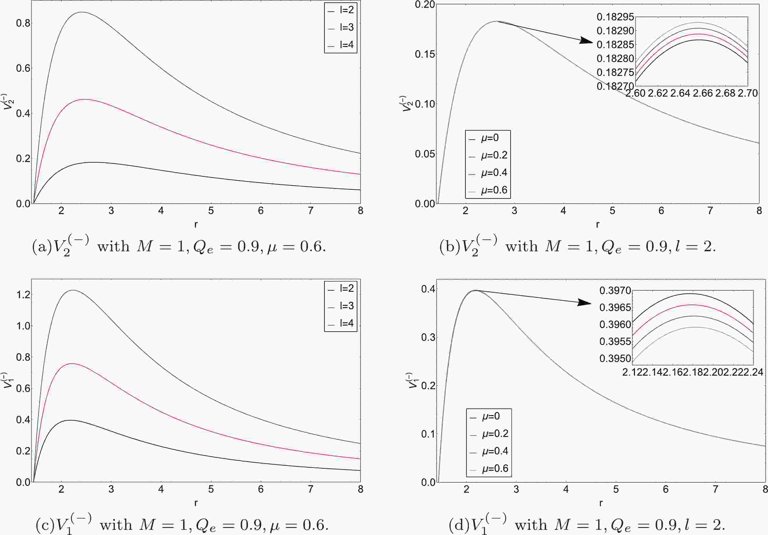
$ \mu=0 $ and$Q_{{\rm e}}=0$ , the equation governing$ Z_{1}^{(-)} $ ,$ Z_{2}^{(-)} $ reduces to the pure EM perturbations and the pure axial gravitational (Regge-Wheeler) perturbations of a Schwarzschild BH, respectively.In Fig. 1, as the multipole number l increases, the height of the potential increases. In addition, one can see that as the value of μ increases, the height of the potential
$ V_{2}^{(-)} $ increases slightly, while$ V_{1}^{(-)} $ shows the opposite trend.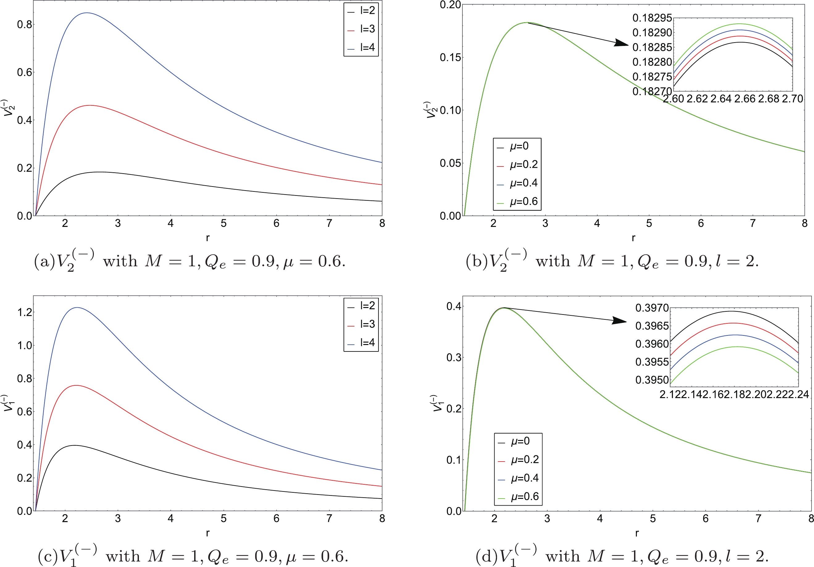
Figure 1. (color online) Behavior of the EEH BH effective potential
$ V_{i}^{(-)} $ under axial gravitational perturbations: (a), (c) different values of l (from bottom to top:$ l=2,3,4 $ ), (b) different values of μ (from bottom to top:$ \mu=0,0.2,0.4,0.6 $ ), (d) different values of μ (from bottom to top:$ \mu=0.6,0.4,0.2,0 $ ). -
The non-vanishing increments of ν,
$ \mu_{2} $ ,$ \mu_{3} $ , and ψ (i.e.,$ \delta \nu $ ,$ \delta \mu_{2} $ ,$ \delta \mu_{3} $ , and$ \delta \psi $ ) denote polar perturbations of the EEH solution. By linearizing expressions for$ R_{02} $ ,$ R_{03} $ ,$ R_{23} $ ,$ R_{11} $ , and$ G_{22} $ about the EEH BH Eq. (14), we can obtain the following equations$ \left(\delta \psi+\delta \mu_{3}\right)_{, r}+\left(\frac{1}{r}-\nu_{, r}\right)\left(\delta \psi+\delta \mu_{3}\right)-\frac{2}{r} \delta \mu_{2}=0, $

(42) $ \begin{aligned}[b] & (\left(\delta \psi+\delta \mu_{2}\right)_{, \theta}+\left(\delta \psi-\delta \mu_{3}\right) \cot \theta)_{, 0}\\=& \frac{P_{23} {\rm e}^{\nu } \left(\mu Q_{\rm e}^2-2 r^4 Q_{\rm e}\right)}{r^5}, \end{aligned} $

(43) $ \begin{split} &(\delta \psi+\delta \nu)_{, r, \theta}+(\delta \psi-\delta \mu_{3})_{, r} \cot \theta \\& +\left(\nu_{, r}-\frac{1}{r}\right) \delta \nu_{, \theta}-\left(\nu_{, r}+\frac{1}{r}\right) \delta \mu_{2, \theta}\\ =&\frac{P_{03} {\rm e}^{-\nu } \left(\mu Q_{\rm e}^3-2 r^4 Q_{\rm e}\right)}{r^5}, \end{split} $

(44) $ \begin{split} &{\rm e}^{2 \nu}\left(\frac{2}{r} \delta \nu_{, r}+\left(\frac{1}{r}+\nu_{, r}\right)\left(\delta \psi+\delta \mu_{3}\right)_{, r}-2\left(\frac{1}{r^{2}}+2 \frac{\nu_{, r}}{r}\right) \delta \mu_{2}\right)\\ &+\frac{1}{r^{2}}((\delta \psi+\delta \nu)_{, \theta, \theta}+\left(2 \delta \psi+\delta \nu-\delta \mu_{3}\right)_{, \theta} \cot \theta+2 \delta \mu_{3}) \\ &-{\rm e}^{-2 \nu}\left(\delta \psi+\delta \mu_{3}\right)_{, 0,0}=\frac{\delta P_{02} \left(2 r^4 Q_{\rm e}-\mu Q_{\rm e}^3\right)}{r^6}, \end{split} $

(45) and
$ \begin{aligned}[b] &{\rm e}^{2 \nu}(2\left(\frac{1}{r}+\nu_{, r}\right) \delta \psi_{, r}-2\left(\frac{1}{r}+2 \nu_{, r}\right) \frac{\delta \mu_{2}}{r}+\delta \psi_{, r, r}\\ &+\frac{1}{r}\left(\delta \psi+\delta \nu+\delta \mu_{3}-\delta \mu_{2}\right), r)+\frac{1}{r^{2}}(\delta \psi_{, \theta, \theta}+\delta \psi_{, \theta} \cot \theta\\ &+2 \delta \mu_{3}+\left(\delta \psi+\delta \nu-\delta \mu_{3}+\delta \mu_{2}\right)_{, \theta} \cot \theta) -{\rm e}^{-2 \nu} \delta \psi_{, 0,0}\\ = &\frac{\delta P_{02} \left(2 r^4 Q_e-3 \mu Q_{\rm e}^3\right)}{r^6}. \end{aligned} $

(46) Eqs. (42)–(46) must be considered alongside Eq. (21) obtained from the linearization of EM field equations.
The variables r and θ in Eqs. (21) and (42)–(46) can be separated by substitutions:
$ \begin{split} & \delta \nu=N(r) P_{l}(\theta), \delta \mu_{2}=L(r) P_{l}(\theta),\\ & \delta \mu_{3}=\left[T(r) P_{l}+V(r) P_{l, \theta, \theta}\right], \\ & \delta \psi=\left[T(r) P_{l}+V(r) P_{l, \theta} \cot \theta\right],\end{split} $

$ \begin{split} & \delta P_{02}=\frac{r^{2} {\rm e}^{2 \nu}}{2 Q_{\rm e}} B_{02}(r) P_{l}, \\ & P_{03}=-\frac{r {\rm e}^{\nu}}{2 Q_{\rm e}} B_{03}(r) P_{l, \theta},\\ & P_{23}=-{\rm i} \sigma \frac{r {\rm e}^{-\nu}}{2 Q_{\rm e}} B_{23}(r) P_{l, \theta}. \end{split} $

(47) As a result, according to Eqs. (47),
$ \left[\frac{\mathrm{d}}{\mathrm{d} r}+\left(\frac{1}{r}-\nu_{, r}\right)\right][2 T-l(l+1) V] -\frac{2}{r} L=0, $

(48) $ (T-V+L)=\left(1-\frac{\mu Q_{\rm e}^2}{2 r^4}\right)B_{23}, $

(49) $ (T-V+N)_{, r}-\left(\frac{1}{r}-\nu_{, r}\right) N -\left(\frac{1}{r}+\nu_{, r}\right) L=\left(1-\frac{\mu Q_{\rm e}^2}{2 r^4}\right)B_{03}, $

(50) $ \begin{aligned}[b] &\frac{2}{r} N_{, r}+(\frac{1}{r}+\nu_{, r})[2 T-l(l+1) V] -\frac{2}{r}\left(\frac{1}{r}+2 \nu_{, r}\right) L\\ &-\frac{l(l+1)}{r^{2}} {\rm e}^{-2 \nu} N -\frac{2 n}{r^{2}} {\rm e}^{-2 \nu} T+\sigma^{2} {\rm e}^{-4 \nu}[2 T-l(l+1) V]\\ =&\left(1-\frac{\mu Q_{\rm e}^2}{2 r^4}\right)B_{02}, \end{aligned} $

(51) $ B_{03}=\frac{1}{r^{2}}\left(r^{2} B_{23}\right),_{r}=B_{23, r}+\frac{2}{r} B_{23}, $

(52) $ r^{4} {\rm e}^{2 \nu} B_{02}=2 Q_{\rm e}^{2}[2 T-l(l+1) V]-l(l+1) r^{2} B_{23}, $

(53) and
$ \begin{aligned}[b] \left(r^{2} {\rm e}^{2 \nu} B_{03}\right)_{, r}+r^{2} {\rm e}^{2 \nu} B_{02} =\sigma^{2} r^{2} {\rm e}^{-2 \nu} B_{23}+2 Q_{\rm e}^{2} \frac{N+L}{r^{2}}, \end{aligned} $

(54) where
$ X=n V=(l-1)(l+2) V/2 $ . In addition, Eqs. (49) and (53) are algebraic.We find Eq. (49) can be rewritten as
$ 2 T-l(l+1) V =-2\left(L+X-B_{23}+\frac{\mu Q_{\rm e}^2}{2 r^4}B_{23}\right). $

(55) With Eq. (55), Eq. (48) can be rewritten as
$ \begin{split} &\left(L+X-B_{23}+\frac{\mu Q_{\rm e}^2}{2 r^4}B_{23}\right)_{, r}\\ =&-\left(\frac{1}{r}-\nu_{, r}\right)\left(L+X-B_{23}+\frac{\mu Q_{\rm e}^2}{2 r^4}B_{23}\right)-\frac{1}{r} L. \end{split} $

(56) Similarly, by combining Eqs. (49), (50), and (52)
$ \begin{split} N_{, r}-L_{, r}=&\left(\frac{1}{r}-\nu_{, r}\right) N+\left(\frac{1}{r}+\nu_{, r}\right) L\\ &+\frac{2 r^4-3 \mu Q_{\rm e}^2}{r^5} B_{23}+\left(1-\frac{\mu Q_{\rm e}^2}{2 r^4}\right)B_{03}. \end{split} $

(57) Additionally, by separating variables in Eq. (46) by substituting Eq. (47), we can obtain the equation
$ V_{, r, r}+2\left(\frac{1}{r}+\nu_{, r}\right) \nu_{, r}+\frac{{\rm e}^{-2 \nu}}{r^{2}}(N+L)+\sigma^{2} {\rm e}^{-4 \nu} V=0 $

(58) We may note that Eqs. (51), (56), and (57) are three first order linear equations of three functions N, L, and X. These equations can be rewritten as
$ N_{, r}=a N+b L+cX-cB_{23}+c\frac{\mu Q_{\rm e}^2}{2 r^4}, $

(59) $ \begin{aligned}[b] L_{, r}=&\left(a-\frac{1}{r}+\nu_{, r}\right) N+\left(b-\frac{1}{r}-\nu_{, r}\right) L \\ &+c\left(X-B_{23}\right)-\frac{2}{r} B_{23}+\frac{3 \mu Q_{\rm e}^2}{r^5}B_{23}, \end{aligned} $

(60) $ \begin{aligned}[b] X_{, r}=&-\left(a-\frac{1}{r}+\nu_{, r}\right) N-\left(b+\frac{1}{r}-2 \nu_{, r}\right) L\\ &-\left(c+\frac{1}{r}-\nu_{, r}\right)\left(X-B_{23}\right)+B_{03}-\frac{\mu Q_{\rm e}^2}{2 r^4}B_{03}, \end{aligned} $

(61) where
$ a=\frac{n+1}{r} {\rm e}^{-2 \nu}, $

(62) $ \begin{aligned}[b] b =&-\frac{1}{r}-\frac{n}{r} {\rm e}^{-2 \nu}+\nu_{, r}+r \nu_{, r}^{2}+\sigma^{2} r {\rm e}^{-4 \nu}\\ &-2 \frac{Q_{\rm e}^{2}}{r^{3}} {\rm e}^{-2 \nu}+\frac{\mu {\rm e}^{-2 \nu } Q_{\rm e}^4}{r^7} , \end{aligned} $

(63) $ \begin{aligned}[b] c =&-\frac{1}{r}+\frac{{\rm e}^{-2 \nu}}{r}+r \nu_{, r}^{2}+\sigma^{2} r {\rm e}^{-4 \nu}\\ &-2 \frac{Q_{{\rm e}}^{2}}{r^{3}} {\rm e}^{-2 \nu}+\frac{\mu {\rm e}^{-2 \nu } Q_{\rm e}^4}{r^7} . \end{aligned} $

(64) According to the method by Chandrasekhar and Xanthopoulos, Eqs. (52)–(54) and (59)–(61) can be reduced to two independent second order equations with functions
$ H_{2}^{(+)} $ and$ H_{1}^{(+)} $ as follows$ H_{2}^{(+)}=\frac{r}{n} X-\frac{r^{2}}{\varpi}\left(L+X-\frac{\mu B_{23} Q_{\rm e}^2}{2 r^4}+B_{23}\right), $

(65) and
$ \begin{aligned} H_{1}^{(+)} =-\frac{1}{Q_{\rm e} \mu}\left[r^{2} B_{23}+2 \frac{Q_{e}^{2}}{r}\left(\frac{r}{n} X-H_{2}^{(+)}\right)\right], \end{aligned} $

(66) where
$\varpi=n r+3 M+\mu Q_{\rm e}^4/5 r^5-2 Q_{\rm e}^2/r$ . Moreover, the pair of equations reads below:$ \begin{aligned}[b] \Lambda^{2} H_{2}^{(+)}=&\frac{\Delta}{r^{5}}[U H_{2}^{(+)}+W(- \left(\frac{\mu Q_{\rm e}^4}{5 r^5}+3 M\right) H_{2}^{(+)}\\ &+ \left(2-\frac{\mu Q_{\rm e}^2}{r^4}\right) \mu H_{1}^{(+)})], \end{aligned} $

(67) $ \begin{aligned}[b] \Lambda^{2} H_{1}^{(+)}=&\frac{\Delta}{r^{5}}[U H_{1}^{(+)}+W(+2 Q_{{\rm e}} \mu H_{2}^{(+)}\\ &+ \left(3 M-\frac{2 \mu Q_{\rm e}^4}{r^5}\right) H_{1}^{(+)})], \end{aligned} $

(68) where
$ \begin{split} &U=(2 n r+3 M) W+(\varpi-n r-M)-\frac{2 n \Delta}{\varpi},\\ &W=\frac{\Delta}{r \varpi^{2}}(2 n r+3 M)+\frac{1}{\varpi}(n r+M). \end{split} $

(69) As with axial perturbations, for polar perturbations Eqs. (67) and (68) can be decoupled by
$ \begin{split} &Z_{1}^{(+)}=+q_{1} H_{1}^{(+)}+\left(-q_{1} q_{2}\right)^{1 / 2} H_{2}^{(+)},\\ &Z_{2}^{(+)}=-\left(-q_{1} q_{2}\right)^{1 / 2} H_{1}^{(+)}+q_{1} H_{2}^{(+)}, \end{split} $

(70) where
$ q_{1} $ and$ q_{2} $ are defined in Eqs. (37) and (38). Finally, one-dimensional wave equations read$ \Lambda^{2} Z_{i}^{(+)}=V_{i}^{(+)} Z_{i}^{(+)} \quad(i=1,2), $

(71) where
$ \begin{split} &V_{1}^{(+)}=\frac{\Delta}{r^{5}}\left[U+\frac{1}{2}\left(q_{1}-q_{2}\right) W\right],\\ &V_{2}^{(+)}=\frac{\Delta}{r^{5}}\left[U-\frac{1}{2}\left(q_{1}-q_{2}\right) W\right]. \end{split} $

(72) It can be observed that in the limit of
$ \mu=0 $ and$ Q_{\rm e}=0 $ , the equation governing$ Z_{1}^{(+)}, Z_{2}^{(+)} $ reduces to the pure EM perturbations and the pure polar gravitational (Zerlli) perturbations of a Schwarzschild BH, respectively.In Fig. 2, as the multipole number l increases, the height of the potential increases. In addition, one can see that as the value of μ increases, the height of the potential
$ V_{2}^{(+)} $ increases slightly, while$ V_{1}^{(+)} $ shows the opposite trend.
Figure 2. (color online) The behavior of the EEH BH effective potential
$ V_{i}^{(+)} $ under polar gravitational perturbations: (a), (c) different values of l (from bottom to top:$ l=2,3,4 $ ), (b) different values of μ (from bottom to top:$ \mu=0,0.2,0.4,0.6 $ ), (d) different values of μ (from bottom to top:$ \mu=0.6,0.4,0.2,0 $ ).As indicated to the left of Fig. 3, we show the potential barriers
$ V_{2}^{(\pm)} $ surrounding the EEH BH: the solid blue curves and the red dashed curves are appropriate for both the axial perturbations and the polar perturbations, respectively. The potential barriers for the polar perturbations differ very little from those of the axial perturbations. The potential barriers$ V_{1}^{(\pm)} $ surrounding the EEH BH are shown in the right of Fig. 3: solid blue curves and red dashed curves are appropriate for both the axial and the polar perturbations, respectively. In the scale of the figure, we cannot distinguish the potential barriers for the axial perturbations from those for the polar perturbations.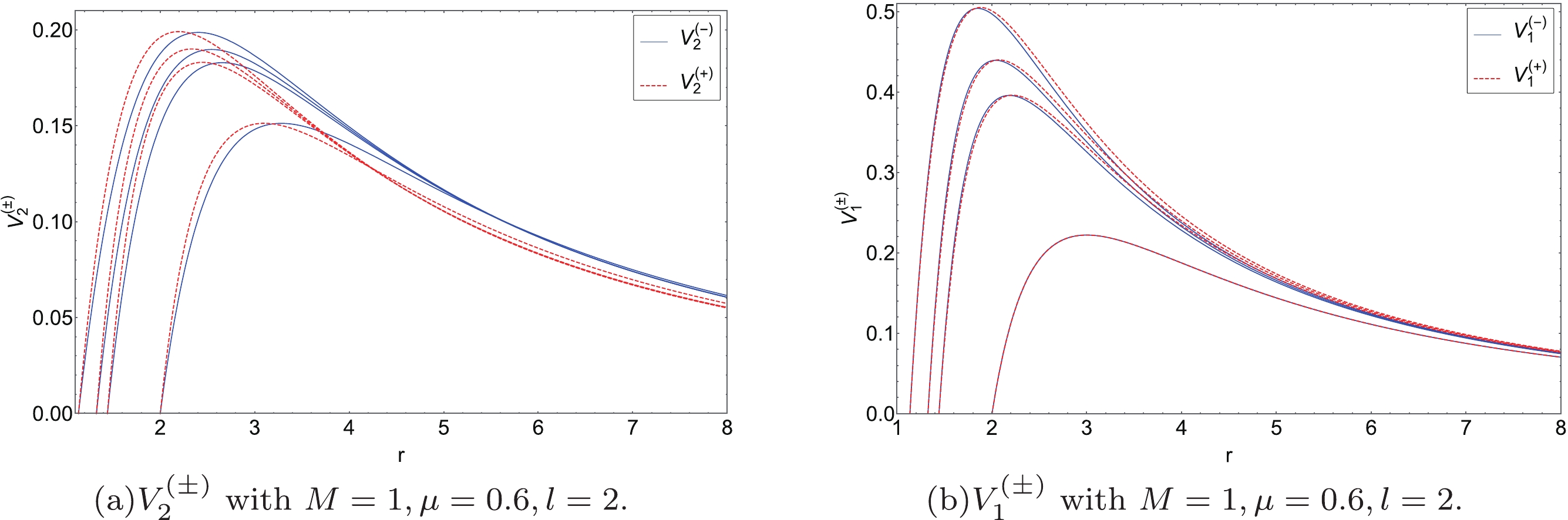
Figure 3. (color online) The relation between the polar effective potential
$ V_{i}^{(+)} $ and the axial effective potential$ V_{i}^{(-)} $ of the EEH BH. Curves are labelled by values of$Q_{\rm e}=0,0.9,0.95$ and$ 1 $ to which they belong. -
To calculate the quasinormal frequencies of both the axial and the polar gravitational perturbations, there are many methods, such as semi-analytic methods [17, 19] and numerical approaches [43, 44]. In this study, the 6th order WKB method was used to obtain the quasinormal frequencies. This method was first suggested in [35] and up to the 3rd order beyond the eikonal approximation [36]. Konoplya and Zhidenko used the 6th order WKB method to solve the scattering problem [16, 37]. Recently, the 13th order WKB method was proposed in [38]. Specifically, the quasinormal frequencies can be calculated as follows [35–37]
$ \frac{{\rm i}\left(\omega^{2}-V_{m}\right)}{\sqrt{-2 V_{m}^{\prime \prime}}}-\sum\limits_{i=2}^{6} \Lambda_{i}=n+\frac{1}{2}, $

(73) where
$ \Lambda_{i} $ are constant coefficients derived from higher order WKB corrections, and$ V_{m} $ and$ V_{m}^{\prime \prime} $ represent the maximum of the potential and its second derivative, respectively. In this paper, we will focus on the fundamental QNMs with the overtone number$ n = 0 $ . -
Table 1 lists the quasinormal frequencies of both the axial and the polar gravitational perturbations in the EEH BH spacetime. The sign of the real (imaginary) parts of the quasinormal frequencies is positive (negative). The real parts of quasinormal frequencies describe the oscillation of gravitational perturbations, while the imaginary parts of those frequencies describe the decay of amplitudes. We mainly focus on the impact of the EH parameter μ while
$ l=2,3,4 $ . The results illustrate μ would increase the real parts of the quasinormal frequencies$ \operatorname{Re}(\omega) $ for$ V_{2}^{(\pm)} $ but decrease them for$ V_{1}^{(\pm)} $ . Meanwhile, the EH parameter μ would increase the imaginary parts of the quasinormal frequencies$ \operatorname{Im}(\omega) $ for$ V_{1}^{(\pm)} $ and$ V_{2}^{(+)} $ but decrease them for$ V_{2}^{(-)} $ . The behavior of the axial gravitational QNMs is different from that of the polar gravitational QNMs for varying EH parameter μ. Another interesting fact is that the axial sector and the polar section (i.e.,$ V_{2}^{(-)} $ and$ V_{2}^{(+)} $ ,$ V_{1}^{(-)} $ and$ V_{1}^{(+)} $ ) share very close spectra in Table 1. In other words, the isopectrality remains unbroken in the gravitational perturbations of the EEH BH. In fact, the isopectrality applies to the Schwarzschild, RN and Kerr BH [30, 31, 34]. However, for the modified gravity theories, the isospectrality is generally broken [45–53]. From this point of view, the isospectrality of the EEH BH is interesting.l μ Axial Polar $ V_{2}^{(-)} $ 

$ V_{1}^{(-)} $ 

$ V_{2}^{(+)} $ 

$ V_{1}^{(+)} $ 

2 0 0.381624 - 0.0895441 i 0.493673 - 0.0972002 i 0.381692 - 0.0896098 i 0.493673 - 0.0972000 i 0.1 0.381625 - 0.0895437 i 0.493670 - 0.0972016 i 0.381694 - 0.0896102 i 0.493670 - 0.0972011 i 0.2 0.381627 - 0.0895433 i 0.493665 - 0.0972032 i 0.381696 - 0.0896106 i 0.493667 - 0.0972022 i 0.3 0.381628 - 0.0895430 i 0.493662 - 0.0972048 i 0.381698 - 0.0896110 i 0.493664 - 0.0972033 i 0.4 0.381630 - 0.0895425 i 0.493657 - 0.0972064 i 0.381699 - 0.0896114 i 0.493661 - 0.0972044 i 0.5 0.381632 - 0.0895420 i 0.493654 - 0.0972078 i 0.381701 - 0.0896117 i 0.493658 - 0.0972055 i 3 0 0.612651 - 0.0932423 i 0.705399 - 0.0976511 i 0.612651 - 0.0932428 i 0.705399 - 0.0976511 i 0.1 0.612653 - 0.0932421 i 0.705395 - 0.0976525 i 0.612653 - 0.0932427 i 0.705396 - 0.0976522 i 0.2 0.612655 - 0.0932420 i 0.705391 - 0.0976539 i 0.612655 - 0.0932426 i 0.705392 - 0.0976534 i 0.3 0.612656 - 0.0932419 i 0.705387 - 0.0976553 i 0.612658 - 0.0932425 i 0.705389 - 0.0976545 i 0.4 0.612658 - 0.0932417 i 0.705383 - 0.0976567 i 0.612660 - 0.0932425 i 0.705385 - 0.0976556 i 0.5 0.612660 - 0.0932416 i 0.705379 - 0.0976581 i 0.612662 - 0.0932424 i 0.705381 - 0.0976568 i 4 0 0.828575 - 0.0947359 i 0.913104 - 0.0977910 i 0.828575 - 0.0947359 i 0.913104 - 0.0977910 i 0.1 0.828577 - 0.0947359 i 0.913099 - 0.0977923 i 0.828577 - 0.0947359 i 0.913099 - 0.0977921 i 0.2 0.828579 - 0.0947358 i 0.913095 - 0.0977935 i 0.828580 - 0.0947358 i 0.913095 - 0.0977932 i 0.3 0.828581 - 0.0947358 i 0.913090 - 0.0977948 i 0.828582 - 0.0947358 i 0.913091 - 0.0977943 i 0.4 0.828583 - 0.0947357 i 0.913086 - 0.0977960 i 0.828584 - 0.0947358 i 0.913087 - 0.0977954 i 0.5 0.828585 - 0.0947357 i 0.913082 - 0.0977973 i 0.828586 - 0.0947357 i 0.913083 - 0.0977965 i Table 1.
$ V_{i}^{(\pm)} $ with$ M=1 $ ,$Q_{{\rm e}}=0.5.$ Furthermore, we calculate the quasinormal frequency ratio of the EEH BH and the RN BH to highlight the effect of the EH parameter μ. In Fig. 4, the solid curves represent the real quasinormal frequency ratio of the EEH BH and the RN BH, while the dashed curves represent the imaginary quasinormal frequency ratio. We set
$ M=1,l=2 $ for the effective potential$ V_{i}^{(\pm)} $ in this figure. The ratios are calculated for the EH parameter μ. Different curves correspond to different values of$Q_{\rm e}=0,0.3,0.4,0.5$ . Fig. 4 also shows that the charge$Q_{\rm e}$ increases the influence of the EH parameter μ.
Figure 4. (color online)
$ V_{i}^{(\pm)} $ with$ M=1,\; l=2,\; \mu=0.5 $ . Real parts (solid curves) and imaginary parts (dashed curves) of the quasinormal frequency ratio between the EEH BH and the RN BH are shown with respect to μ. -
According to Cardoso et al. [54], in the eikonal limit, the real and imaginary parts of the QNMs of an SSS flat spacetime are given as follows:
$ \omega = \Omega_{c} l-{\rm i}(n+1 / 2)\left|\lambda_{c}\right|, $

(74) where
$ \Omega_{c}=\frac{f_{c}^{1 / 2}}{r_{c}}, $

(75) and
$ \lambda_{c}=\frac{1}{\sqrt{2}} \sqrt{-\frac{r_{c}^{2}}{f_{c}}\left(\frac{{\rm d}^{2}}{{\rm d} r_{*}^{2}} \frac{f(r)}{r^{2}}\right)_{r=r_{c}}}. $

(76) $ \Omega_{c} $ and$ \lambda_{c} $ are the angular velocity and the Lyapunov exponent of the unstable circular null geodesics (i.e., the light ring), respectively.$ r_{c} $ is the radius of the circular null geodesic, and it satisfies$ 2 f_{c}=r_{c} f_{c}^{\prime} $ .$ r_{*} $ is the tortoise coordinate and defined by$ {\rm d} r/{\rm d} r_{*}=f(r) $ . However, there is a counter-example in [55] that Eq. (74) is invalid in the Einstein-Lovelock theory. In this paper, we shall use the same method in [55] to check that Eq. (74) is not violated in the gravitational perturbations of the EEH BH.On the one hand, in order to obtain concise analytical expressions of
$ \Omega_{c} $ and$ \lambda_{c} $ , it is necessary to expand$ r_{c} $ in terms of μ as follows:$ r_{c}=r_{c 0}+r_{c 1} \mu+\mathcal{O}\left(\mu^{2}\right) . $

(77) The equation
$ 2 f_{c}=r_{c} f_{c}^{\prime} $ reads$ 10 r^{6}-30 M r^{5}+20 Q_{\rm e}^{2} r^{4}-2 \mu Q_{\rm e}^{4}=0 $

(78) Substituting Eq. (77) into Eq. (78), one can find the following:
$ \begin{aligned}[b] &r_{c0}=\frac{1}{2}\left(3 M+\sqrt{9 M^{2}-8 Q_{\rm e}^{2}}\right), \\ &r_{c1}=\frac{16 Q_{\rm e}^{4}\left(3 M+\sqrt{9 M^{2}-8 Q_{\rm e}^{2}}\right)^{-3}}{5\left(9 M^{2}-8 Q_{\rm e}^{2}+3 M \sqrt{9 M^{2}-8 Q_{\rm e}^{2}}\right)}. \end{aligned} $

(79) It is interesting from Eq. (79) that
$ r_{c0} $ is actually the radius$ r_{cRN} $ of the circular null geodesic of the RN BH. One can then also expand$ \Omega_{c} $ and$ \lambda_{c} $ (given by Eq. (75) into Eq. (76)) in terms of a as follows:$ \begin{split} \Omega_{c}=\frac{\sqrt{M r_{c0}-Q_{\rm e}^{2}}}{r_{c0}^{2}}-\frac{Q_{\rm e}^{4}}{40 r_{c0}^{6} \sqrt{M r_{c0}-Q_{\rm e}^{2}}} \mu+ \mathcal{O}\left(\mu^{2}\right), \end{split} $

(80) and
$ \begin{split} \lambda_{c} =&\sqrt{\frac{\alpha_{1}}{2 r_{c0}^{6}}}+\frac{ \sqrt{\alpha_{1}}\left(17 Q_{\rm e}^{4} \alpha_{1}+\alpha_{2}\right)}{80 \sqrt{2} r_{c0}^{7}\left(4 Q_{\rm e}^{2}-3 M r_{c0}\right)^{2}\left(M r_{c0}-Q_{\rm e}^{2}\right)} \mu \\ & + \mathcal{O}\left(\mu^{2}\right), \end{split} $

(81) where parameters
$ \alpha_{1} $ and$ \alpha_{2} $ are given as follows:$ \begin{split} \alpha_{1} =&27 M^{4}-33 M^{2} Q_{\rm e}^{2}+8 Q_{\rm e}^{4}\\ &+9 M^{3} \sqrt{9 M^{2}-8 Q_{\rm e}^{2}}-7 M Q_{\rm e}^{2} \sqrt{9 M^{2}-8 Q_{\rm e}^{2}} , \\ \alpha_{2}=&Q_{\rm e}^{6}\left(57 M^{2}-40 Q_{\rm e}^{2}+19 M \sqrt{9 M^{2}-8 Q_{\rm e}^{2}}\right). \end{split} $

(82) It is clear from Eqs. (80) and (81) that the quasinormal frequencies are related to the first order terms of the EH parameter μ. In the case of
$ \mu=0 $ , the quasinormal frequencies can go to back to the case of the RN BH.On the other hand, in the eikonal limit, for the effective potential
$ V_{i}^{(\pm)} $ of master Eqs. (40) and (71), one can find that$ \lim \limits_{l \rightarrow \infty} \frac{V_{i}^{(\pm)}}{V_{\rm eikonal}}=1, $

(83) where
$ V_{\rm eikonal} = f(r) \frac{l^{2}}{r^{2}}. $

(84) Therefore, in the eikonal limit, the effective potential
$ V_{i}^{(\pm)} $ can be rewritten as follows:$ V_{i}^{(\pm)}= l^{2}\left(\frac{f(r)}{r^{2}}+\mathcal{O}\left(\frac{1}{\ell}\right)\right). $

(85) According to Schutz and Will [35] (see also [55]), the WKB formula can be applied for finding QNMs as follows:
$ \frac{Q_{0}\left(r_{0}\right)}{\sqrt{2 Q_{0}^{(2)}\left(r_{0}\right)}}=i(n+1 / 2), $

(86) where
$ Q_{0}^{(2)} \equiv {\rm d}^{2} Q_{0} / {\rm d} r_{*}^{2} $ and$ r_{0} $ is the extremum of$ Q_{0} $ . In the eikonal limit, one can find that$ Q_{0} \simeq \omega^{2}-f(r) \frac{l^{2}}{r^{2}}. $

(87) It is easy to find that
$ 2 f\left(r_{0}\right)=r_{0} f^{\prime}\left(r_{0}\right), $

(88) It is clear that if Eq. (88) does coincide with Eq. (74), then
$ r_{0} $ must coincide with$ r_{c} $ . Moreover, the WKB formula is given as follows:$ \omega_{\mathrm{QNM}}=l \sqrt{\frac{f\left(r_{0}\right)}{r_{0}^{2}}}-{\rm i} \frac{(n+1 / 2)}{\sqrt{2}} \sqrt{-\frac{r_{0}^{2}}{f\left(r_{0}\right)}\left(\frac{{\rm d}^{2}}{{\rm d} r_{*}^{2}} \frac{f\left(r\right)}{r^{2}}\right)_{r_{0}}} . $

(89) One can find that Eq. (89) does coincide with Eq. (74). In the eikonal limit, Eq. (74) is not violated in the gravitational perturbations of the EEH BH.
In addition, the quasinormal frequencies cannot go to back to the case of the RN BH when
$ l \rightarrow \infty $ . In other words, in the eikonal approximation, the EEH BH and the RN BH can be distinguished through the QNMs. This is consistent with the case in which the Schwarzschild BH and the RN BH have different QNMs in the eikonal limit [56]. -
In EEH BH spacetime, we study the dynamic evolution of gravitational perturbations and late-time tails through the finite difference method [57–60]. In light-cone coordinates where
$ u=t-r_{*} $ and$ v=t+r_{*} $ , we rewrite master Eqs. (40) and (71) as follows:$ \frac{\partial^{2} \Psi}{\partial u \partial v}+\frac{1}{4} V(r) \Psi=0. $

(90) By imposing appropriate boundary conditions on
$ u=u_{0} $ and$ v=v_{0} $ , Eq. (90) can be calculated by directly integrating numerically.Figure 5 shows the dynamic evolution of both the axial and the polar gravitational perturbations for different multipole numbers
$ l=2,3,4 $ , which shows that no instability occurs. The period of oscillation of the gravitational field and the descent speed of the peak decrease and increase with higher multipole number l, respectively. This result shows the consistency with the analysis of the 6th order WKB method. In the scale of Fig. 6, the dynamic evolution profiles of$ V_{i}^{(\pm)} $ for$ \mu=0,0.2,0.4,0.6 $ have close resemblances so we cannot distinguish them. In other words, the effect of the EH parameter μ on the periods of oscillation and the descent speed of the peak is not obvious.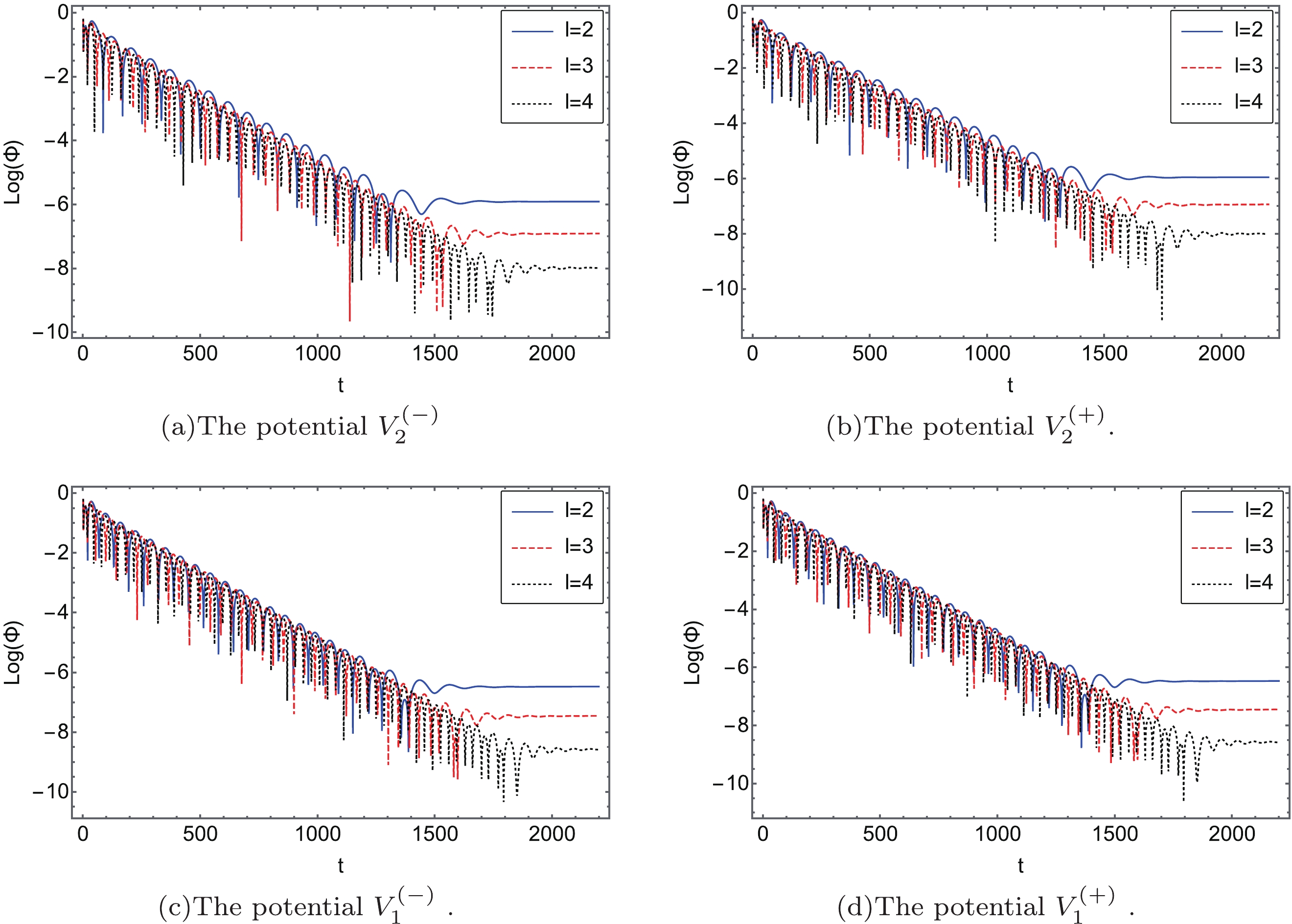
Figure 5. (color online) Dynamical evolution of fundamental QNMs of both axial and polar gravitational perturbations in the EEH BH spacetime with
$M=1,Q_{\rm e}=0.5,\mu=0.6$ and multipole numbers$ l=2,3,4 $ .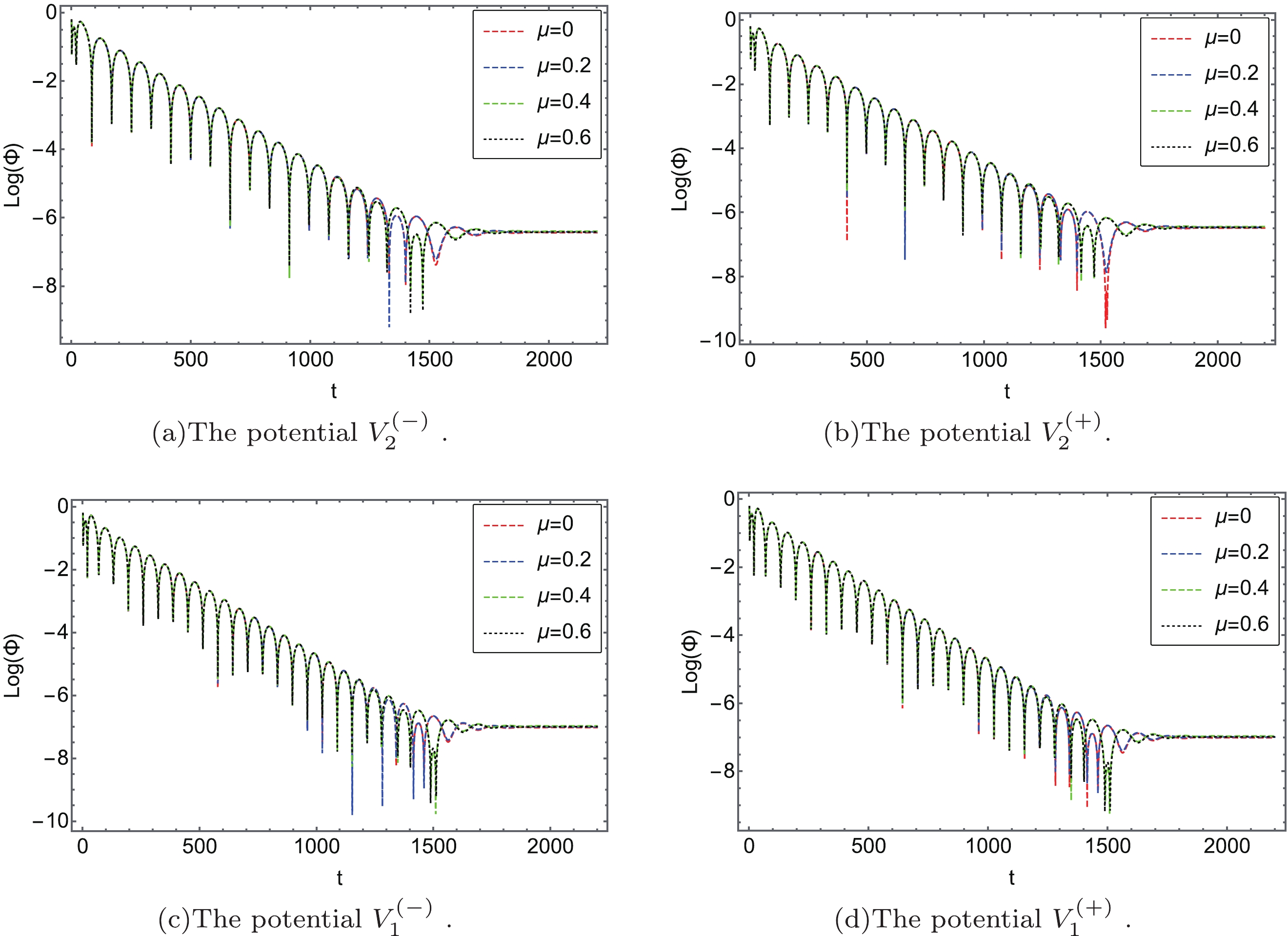
Figure 6. (color online) Dynamical evolution of fundamental QNMs of both axial and polar gravitational perturbations in the EEH BH spacetime with
$M=1,Q_{\rm e}=0.5,l=2$ and EH parameter$ \mu=0,0.2,0.4,0.6 $ . -
We briefly review the EEH BH. The investigation of the QNMs has shown that the EH parameter μ affects the gravitational perturbations of the EEH BH. In the limit of
$ \mu=0 $ and$ Q_{\rm e}=0 $ , the equation governing$ Z_{2}^{(-)}, Z_{2}^{(+)} $ reduces to the pure axial (Regge-Wheeler) and the pure polar gravitational (Zerilli) perturbations of a Schwarzschild BH, respectively, while the equation governing$ Z_{1}^{(-)}, Z_{1}^{(+)} $ reduces to pure EM perturbations. The EH parameter μ enhances the imaginary part$ \operatorname{Re}(\omega) $ for$ V_{2}^{(\pm)} $ , but for$ V_{1}^{(\pm)} $ , the trends reveal the opposite. The EH parameter μ increases the real part$ \operatorname{Im}(\omega) $ for$ V_{1}^{(\pm)} $ and$ V_{2}^{(+)} $ , while for$ V_{2}^{(-)} $ , the opposite is the case. In the gravitational perturbations of the EEH BH, the isopectrality remains unbroken. In our future work, the isospectrality in the modified gravity theories will be discussed in detail. Additionally, the charge$ Q_{e} $ increases the impact of the EH parameter μ. In the eikonal limit, the eikonal quasinormal frequencies correspond to the properties of the null circular orbit around the EEH BH, and the quasinormal frequencies are related to the EH parameter μ. Finally, we study the dynamic evolution of both the axial and the polar gravitational perturbations. This shows that the period of the oscillation in the gravitational field decreases with higher multipole number l. In addition, the perturbation with$ l=2 $ decays thw slowest. In Fig. 6, the dynamic evolution profiles are very similar, so it is difficult to distinguish them. In fact, the conclusion is consistent with the case in which their effective potentials are almost identical.
Gravitational perturbations of the Einstein-Euler-Heisenberg black hole
- Received Date: 2022-02-25
- Available Online: 2022-08-15
Abstract: The prospect of using gravitational wave detections via the quasinormal modes (QNMs) to test modified gravity theories is exciting area of current research. Gravitational waves (GWs) emitted by a perturbed black hole (BH) will decay as a superposition of their QNMs of oscillations at the ringdown phase. In this work, we investigate the QNMs of the Einstein-Euler-Heisenberg (EEH) BH for both axial and polar gravitational perturbations. We obtain master equations with the tetrad formalism, and the quasinormal frequencies of the EEH BH are calculated in the 6th order Wentzel-Kramers-Brillöuin approximation. It is interesting to note that the QNMs of the EEH BH would differ from those of the Reissner-Nordström BH under the EH parameter, which indicates the EH parameter would affect the gravitational perturbations for the EEH BH.


 DownLoad: