


 Abstract
 HTML
HTML Reference
 Related
 PDF
PDF


-
The nuclear charge radius, which can reflect the nuclear charge density distribution and the Coulomb potential, is one of the most fundamental properties of the atomic nucleus. It depends sensitively on the properties of nuclear force and plays a key role in investigating nuclear structure such as shape coexistence and shape transition [1, 2], shell evolution [3–5], and the nuclear volume properties connected with exotic phenomena such as skin and halo [6–8], etc. Accurate nuclear charge radii are also needed in many theoretical studies, such as understanding the origin of elements in the universe [9, 10].
Experimentally, considerable efforts have been devoted to the measurement of nuclear charge radii. By using several techniques [11, 12], e.g., muonic atom x-ray spectra, electron elastic scattering experiments, and isotope shifts, more than 900 nuclear charge radii have been provided by experiments [13]. Very recently, the observation of the charge radii of several very exotic nuclei has aroused people's attention [14–17], providing a stringent test for various nuclear models.
From theoretical aspects, various methods have been developed to calculate the nuclear charge radii, e.g., phenomenological formulae [18–25], macroscopic–microscopic models [26–29], relativistic [30–37] and non-relativistic [38–40] mean-field models, local-relation-based models [41–46], and ab initio no-core shell model [47]. All of these models can provide global quantitative descriptions for the nuclear charge radii in a wide region of the nuclear chart. However, except for local-relation-based models, the root-mean-square (rms) deviations are larger than 0.02 fm for all of these methods, which need further improvement.
In recent years, machine learning (ML) has been employed to further improve the accuracy of nuclear models, due to its powerful and convenient inference abilities. Various ML approaches have been adopted to improve the description of the nuclear charge radii, e.g., the feed-forward neural network [48, 49], the Bayesian neural network approach [50–53], etc. By training the ML network with the deviations between experimental and calculated charge radii, ML approaches can reduce the corresponding rms deviations significantly to about 0.02 fm.
In this paper, the kernel ridge regression (KRR) method with a Gaussian kernel, which is one of the most popular ML approaches, is used to improve the description of the nuclear charge radius by taking six phenomenological formulae as examples. Least-square fitting based on the Levenberg–Marquardt (LM) method [54] is applied in order to obtain the new parameters in these formulae, and then the KRR method is adopted to train the charge radius residuals. The two hyperparameters (
$ \sigma, \lambda $ ) in the KRR method are determined by leave-one-out cross-validation. The performance and reliability of the extrapolated predictions of the KRR method are also analyzed in detail. The comparison with the radial basis function (RBF) method, which has been widely used to predict the nuclear mass and β-decay half-lives, etc. [55–61], is also discussed. Note that the KRR method has already provided successful descriptions for nuclear mass predictions [62, 63] and also has been used to build nuclear energy density functionals [64].This paper is organized as follows. A brief introduction of the phenomenological nuclear charge radius formulae and the KRR method is presented in Sec. II. The results obtained by the KRR method and the extrapolation power comparison to the RBF method are given in Sec. III. A summary of this work is given in Sec. IV.
-
Considering the nuclear saturation property, the radius of nuclear charge distribution is usually described by the
$ A^{1/3} $ law [18]$ R_c=r_A A^{1/3} \ , $

(1) where A is the mass number and
$ R_c=\sqrt{5/3}\langle r^2 \rangle^{1/2} $ , with$ \langle r^2 \rangle^{1/2} $ the rms nuclear charge radius. In order to obtain the global description of the charge radius, the parameter$ r_A $ is fitted to the experimental data [13]. However, it is found that the$ A^{1/3} $ formula is not valid for all nuclei since$ r_A $ is not a constant but decreases systematically with increasing mass number. Investigations show that$ r_A \approx 1.30 $ fm for light nuclei and 1.20 fm for heavy nuclei. In Ref. [19], a$ Z^{1/3} $ law was proposed$ R_c=r_Z Z^{1/3} \ , $

(2) which is much better than the conventional
$ A^{1/3} $ formula. Investigations show that the parameter$ r_Z $ remains almost constant, i.e.,$ r_Z \approx 1.65 $ fm, for nuclei with$ A \geq 40 $ . Furthermore, the N-dependence of nuclear charge radii was discussed [65] and an$ N^{1/3} $ formula was proposed [25], which can be written as$ R_c=r_N N^{1/3} \ . $

(3) To have a better description of the nuclear charge radii, improved
$ A^{1/3} $ ,$ N^{1/3} $ and$ Z^{1/3} $ formulae that include the isospin dependence have also been proposed [20, 22, 25], which can be written as$ R_c = r_A \left(1-b\frac{N-Z}{A}\right)A^{1/3} \ , $

(4) $ R_c = r_N \left(1-b\frac{N-Z}{N}\right)N^{1/3} \ , $

(5) $ R_c = r_Z \left(1+\frac{5}{8\pi}\beta^2\right)\left(1+b\frac{N-N^\ast}{Z}\right)Z^{1/3} \ , $

(6) where β is the quadrupole deformation, which in the present work is taken from Ref. [66], and
$ N^\ast $ is the neutron number for the nuclei along the β-stability line, which can be extracted from the nuclear mass formula [18] and can be written as$ Z=A/(1.98+0.0155A^{2/3}) $ .$ r_A $ ,$ r_N $ ,$ r_Z $ and b are constants, which are obtained by fitting the experimental data. Note that the influence of deformation on nuclear charge radius was studied systematically in Ref. [67].KRR is a popular ML method with the extension of ridge regression on the nonlinearity [68, 69]. It uses a kernel machine to map data into higher dimensional space and then uses a regression method to treat the data. The KRR function
$ S({\boldsymbol{x}}_j) $ can be written as$ S({\boldsymbol{x}}_j)=\sum\limits_{i=1}^m K({\boldsymbol{x}}_j, {\boldsymbol{x}}_i)\omega_i, $

(7) where m is the number of training data,
$ {\boldsymbol{x}}_i $ denotes the location of training data,$ \omega_{i} $ are weights to be determined, and$ K({\boldsymbol{x}}_j, {\boldsymbol{x}}_i) $ is the kernel function, which characterizes the similarity between the data. There are several kinds of kernels that can be used in the KRR method, e.g., linear kernel, polynomial kernel, Gaussian kernel, etc. In the present work, the Gaussian kernel is adopted,$ K({\boldsymbol{x}}_j,{\boldsymbol{x}}_i)=\exp\left(-\frac{||{\boldsymbol{x}}_i-{\boldsymbol{x}}_j||^2}{2\sigma^2}\right) \ , $

(8) where σ (
$ \sigma>0 $ ) is a hyperparameter defining the range that the kernel affects. By minimizing the following loss function$ L({\boldsymbol{\omega}})=\sum\limits_{i=1}^m [S({\boldsymbol{x}}_i)-y({\boldsymbol{x}}_i)]^2+\lambda||{\boldsymbol{\omega}}||^2 \ , $

(9) the weights
$ \omega_{i} $ can be determined, where$ {\boldsymbol{\omega}} = (\omega_{1},..., \omega_{m}) $ . The hyperparameter λ ($ \lambda\geq0 $ ) determines the regularization strength and is adopted to reduce the risk of overfitting. Minimizing Eq. (9) leads to$ {\boldsymbol{\omega}}=({\boldsymbol{K}}+\lambda {\boldsymbol{I}})^{-1}{\boldsymbol{y}} \ , $

(10) where
$ {\boldsymbol{I}} $ is the identity matrix and$ {\boldsymbol{K}} $ is the kernel matrix with elements$ K_{ij}=K({\boldsymbol{x}}_j, {\boldsymbol{x}}_i) $ .In the present work, the KRR method is applied for nuclear charge radius predictions. Therefore, the coordinate
$ {\boldsymbol{x}}_i $ of each nucleus is naturally chosen as$ {\boldsymbol{x}}_i=(N_i,Z_i) $ . The Euclidean norm$ r=||{\boldsymbol{x}}_i-{\boldsymbol{x}}_j||=\sqrt{(Z_i-Z_j)^2+(N_i-N_j)^2} $

(11) is defined to be the distance between two nuclei.
-
In this work, 884 experimental data [13] with proton number
$ Z \geq 8 $ and neutron number$ N \geq 8 $ have been adopted for least-square fitting with the Levenberg–Marquardt method to obtain new parameters in these six phenomenological nuclear charge radius formulae. The obtained parameters and the corresponding rms deviations are shown in Table 1. In addition, old parameters and the corresponding rms deviations obtained by previous investigations are also shown for comparison. These old parameters are fitted with the experimental data in Ref. [70] except the two$ N^{1/3} $ formulae. It can be seen that the rms deviations are reduced a little when these new parameters are adopted. By considering the isospin dependence, the descriptions are improved a lot, especially for the$ N^{1/3} $ formula. It seems worth noting that the$ Z^{1/3} $ formula with only one parameter achieves an accuracy of charge radii comparable to those of the two-parameter$ A^{1/3} $ and$ N^{1/3} $ formulae with isospin dependence. Among these six phenomenological formulae, the$ Z^{1/3} $ formula with isospin dependence can reproduce the data best, with a rms deviation of 0.049 fm. Note that the parameters have also been refitted in Ref. [25], with results quite similar to the present work except those in Eq. (6). In addition, the parameters are fitted by the rms charge radius$ \langle r^2 \rangle^{1/2} $ in Ref. [25], which has a factor of$ \sqrt{5/3} $ relative to the parameters in Table 1, including these two$ N^{1/3} $ formulae.Formula Parameters $\Delta_{\rm rms}$ /fm

New parameters $\Delta_{\rm rms}$ /fm

$R_c=r_A A^{1/3}$ 

$r_A$ =1.223 fm [18]

0.094 $r_A$ =1.227 fm

0.093 $R_c=r_N N^{1/3}$ 

$r_N$ =1.472 fm [25]

0.151 $r_N$ =1.470 fm

0.151 $R_c=r_Z Z^{1/3}$ 

$r_Z$ =1.631 fm [19]

0.076 $r_Z$ =1.639 fm

0.072 $R_c=r_A \left[1-b(N-Z)/A\right]A^{1/3}$ 

$r_A$ =1.269 fm;

$b=0.252$ [20]

0.068 $r_A$ =1.282 fm;

$b=0.342$ 

0.065 $R_c=r_N \left[1-b(N-Z)/N\right]N^{1/3}$ 

$r_N$ =1.629 fm;

$b=0.451$ [25]

0.063 $r_N$ =1.623 fm;

$b=0.438$ 

0.063 $R_c=r_Z (1+5\beta^2/8\pi)\left[1+b(N-N^\ast)/Z\right]Z^{1/3}$ 

$r_Z$ =1.631 fm;

$b=0.062$ [22]

0.057 $r_Z$ =1.634 fm;

$b=0.220$ 

0.049 Table 1. Parameters and the root-mean-square deviations (
$\Delta_{\rm rms}$ ) for the six phenomenological nuclear charge radius formulae. Experimental data are taken from [13], with proton number$Z \geq 8$ and neutron number$N \geq 8$ .The KRR function (7) is trained to reconstruct the differences between experimental and calculated nuclear charge radius
$ \Delta R(N, Z)=R^{\rm exp}(N,Z)-R^{\rm cal}(N, Z) $ . Once the weights$ w_i $ are obtained, the reconstructed function$ S(N, Z) $ can be obtained for every nucleus. Therefore, the predicted charge radius for a nucleus with neutron number N and proton number Z is given by$R^{\rm KRR} = R^{\rm cal}(N, Z)+S(N,Z)$ .In the present work, leave-one-out cross-validation is adopted to determine the hyperparameters (
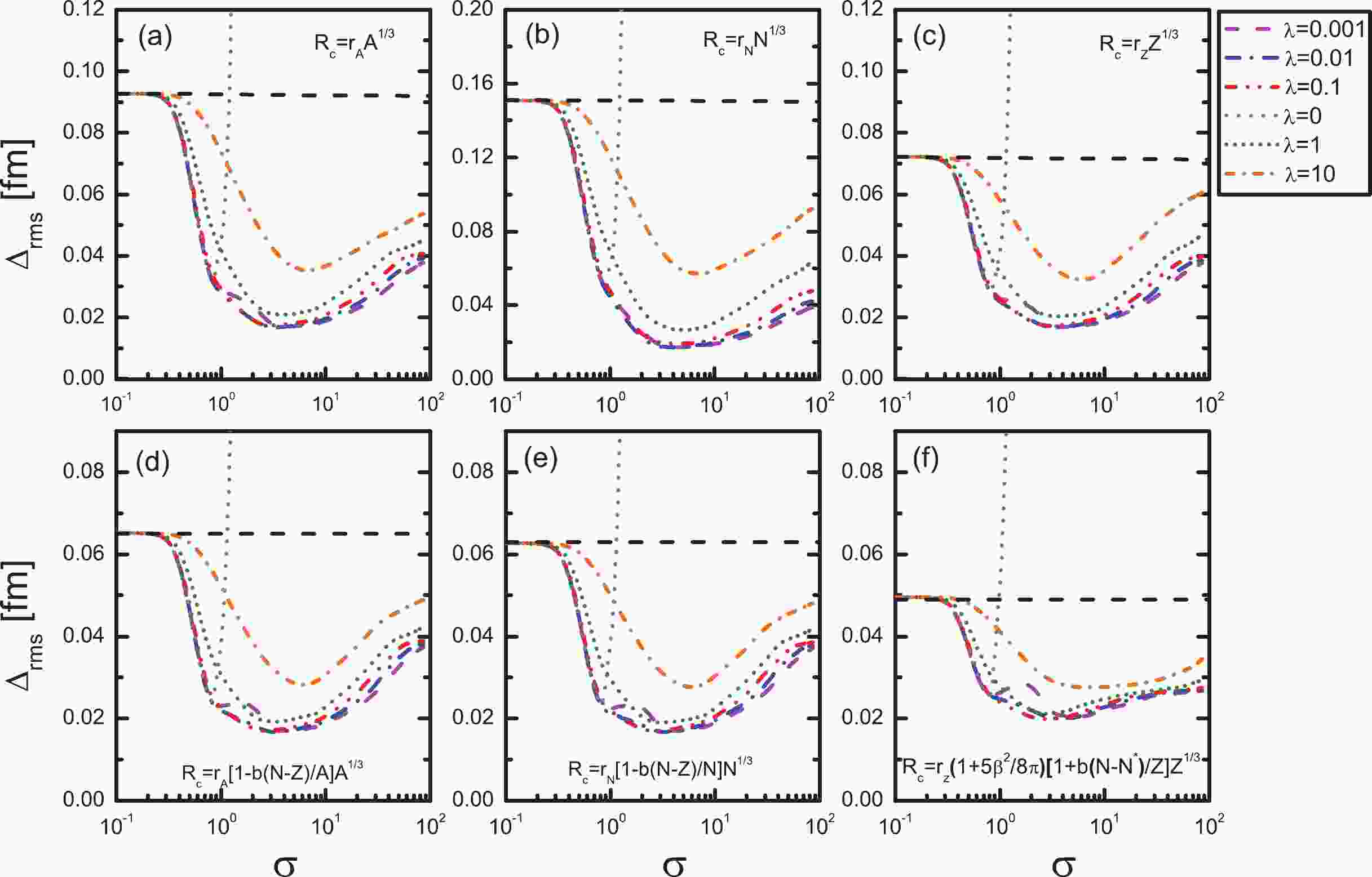
$ \sigma, \lambda $ ). In Fig. 1, the leave-one-out cross-validation rms deviations are presented as a function of the hyperparameter σ with selected penalties λ ranging from$ 10^{-3} $ to$ 10^1 $ . The calculations with$ \lambda=0 $ are also shown, which corresponds to the RBF results. For comparison, the corresponding rms deviation of each formula is also shown with horizontal black dashed lines. It can be seen that for small σ values, the rms deviations obtained by the KRR method are close to those obtained by the phenomenological formulae, regardless of the magnitudes of λ, so the corresponding reconstructed functions$ S(N, Z) $ are quite small. The role of the penalty term can be clearly seen with σ increasing. The penalty λ has a great influence on the selection of the hyperparameter σ. When the penalty term is neglected ($ \lambda=0 $ ), the rms deviations are minimized at$ \sigma=0.83, \; 0.84, \; 0.84, \; 0.82, \; 0.81, \; 0.79 $ for Eqs. (1) to (6), respectively, and they grow rapidly with increasing σ. In addition, the rms deviations obtained with$ \lambda=0 $ are systematically larger than those with the penalty term$ \lambda\neq0 $ . It can be seen that when$ \lambda\neq0 $ , the rms deviations do not grow very fast for a larger σ, in contrary to the case$ \lambda=0 $ , which demonstrates clearly that the penalty term can effectively prevent the results from overfitting.
Figure 1. (color online) The rms deviations as a function of the hyperparameter σ with several selected λ values. For comparison, the corresponding rms deviation of each formula is also shown with horizontal black dashed lines.
It can be seen in Fig. 1 that those minima at
$ \lambda= $ 0.001, 0.01, and 0.1 are quite close to each other. This indicates that the results may not be that sensitive to the hyperparameters in this region. The optimized hyperparameters σ and λ from the KRR method in each formula are shown in Table 2. The obtained rms deviations are smaller than 0.017 fm, except for the$ Z^{1/3} $ formula with isospin dependence, which has a rms deviation with 0.0197 fm. It is quite interesting that this formula can reproduce the data best without the KRR method, but after the KRR modification, the results are the worst of these six formulae. This may be caused by the deformation effect, since the deformation is considered only in this formula. Maybe a better deformation parameter set can further improve the result. It can be seen that the KRR method can enormously improve the description of the nuclear charge radius by these phenomenological formulae, even when the original rms deviation is as large as 0.151 fm in the$ N^{1/3} $ formula. In addition, the predictive power of the KRR method was tested by separating the nuclear charge data into two subsets, i.e., the 782 nuclei in the nuclear charge table of 2004 (denoted as CR04) [70], and the 102 "new" nuclei (denoted as CR13-04) appearing in Ref. [13]. It can be seen that nearly all the rms deviations for the test sets are smaller than 0.03 fm, except for the$ N^{1/3} $ formula.Formula σ λ $\Delta_{\rm rms}^{\rm KRR}/{\rm{ fm} }$ 

$\Delta_{\rm rms}^{\rm CR04}/{\rm{ fm} }$ 

$\Delta_{\rm rms}^{\rm CR13-04}/{\rm{ fm} }$ 

$R_c=r_A A^{1/3}$ 

3.01 0.01 0.0166 0.0125 0.0288 $R_c=r_N N^{1/3}$ 

3.86 0.001 0.0165 0.0128 0.0369 $R_c=r_Z Z^{1/3}$ 

2.93 0.01 0.0168 0.0123 0.0268 $R_c=r_A \left[1-b(N-Z)/A\right]A^{1/3}$ 

2.88 0.01 0.0165 0.0122 0.0280 $R_c=r_N \left[1-b(N-Z)/N\right]N^{1/3}$ 

2.88 0.01 0.0166 0.0122 0.0280 $R_c=r_Z (1+5\beta/8\pi^2)\left[1+b(N-N^\ast)/Z\right]Z^{1/3}$ 

2.46 0.06 0.0197 0.0146 0.0301 Table 2. Adopted hyperparameters σ and λ in the KRR method for each formula obtained through the leave-one-out cross-validation. The corresponding rms deviations between the experimental data and the KRR method are shown as
$\Delta_{\rm rms}^{\rm KRR}$ . The$\Delta_{\rm rms}^{\rm CR04}$ and$\Delta_{\rm rms}^{\rm CR13-04}$ denote the rms deviations of the training and test sets when the nuclear charge radius in Ref. [70] is chosen as the training set (denoted as "CR04"), and the "new" nuclei appearing in Ref. [13] are chosen as the test set (denoted as "CR13-04").When the hyperparameters (
$ \sigma, \lambda $ ) of each formula are determined, the reconstructed function$ S(N,Z) $ for every nucleus can be calculated by KRR method, which are shown in the middle panels of Fig. 2. For comparison, the differences$ \Delta R=R^{\rm exp}-R^{\rm cal} $ between experimental and the calculated values by$ A^{1/3} $ ,$ N^{1/3} $ and$ Z^{1/3} $ formulae are shown in the upper panels of Fig. 2. The magic numbers are shown by vertical and horizontal dotted lines. In the present work, the number of possible existing nuclei with$ Z \geq 8 $ and$ N \geq 8 $ is taken as 7275 according to Ref. [71]. It can be seen clearly that for each formula, the reconstructed function$ S(N,Z) $ has a similar pattern to$ \Delta R $ , which indicates that the charge radius residuals can be learned well by$ S(N,Z) $ . After considering the KRR corrections, the predicted charge radius by these three formulae are in good agreement with the data, which are shown at the lower pannels of Fig. 2. The corresponding rms deviations are reduced to less than 0.017 fm (see Table 2).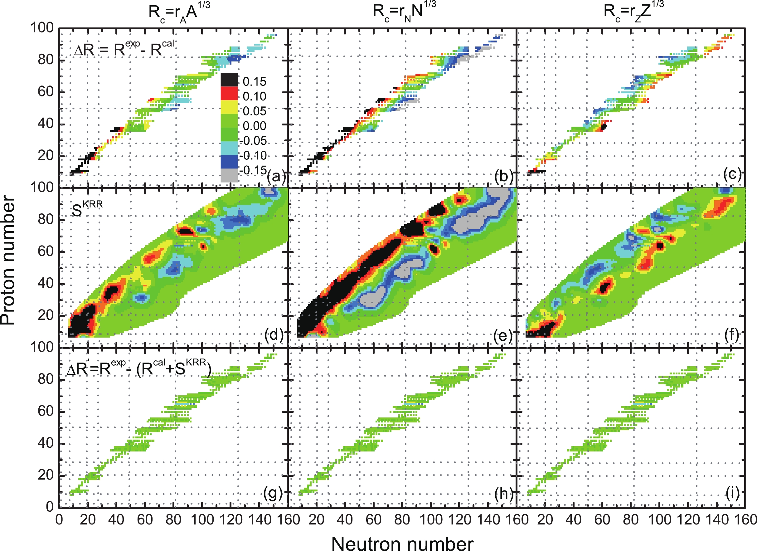
Figure 2. (color online) Differences
$\Delta R=R^{\rm exp}-R^{\rm cal}$ between experimental and the calculated values using$A^{1/3}$ ,$N^{1/3}$ and$Z^{1/3}$ formulae (upper panels), the KRR reconstructed function$S(N, Z)$ (middle panels), and the differences$\Delta R'=R^{\rm exp}-(R^{\rm cal} + S^{\rm KRR})$ between experimental and the predictions of these three formulae with the KRR corrections (lower pannels). The magic numbers are shown by vertical and horizontal dotted lines. The possible existing nuclei are taken from [71].Figure 3 is the same as Fig. 2, but for the three formulae considering the isospin dependence. It can be seen that, after considering the isospin dependence, the descriptions of the experimental data are improved a lot, especially for the
$ N^{1/3} $ formula [see Fig. 3(b)]. After considering the corrections of the reconstructed function, the predicted charge radius (the lower panels of Fig. 3) are quite similar to those corresponding results in Fig. 2. It can be seen in the middle panels of Figs. 2 and 3 that except for those nuclei close to the nuclei with known charge radius, the KRR reconstructed function$ S(N, Z) $ becomes to zero for most nuclei with unknown charge radius. This is due to the Gaussian kernel adopted in the present calculation. It means that for a given nucleus, very little information can be learned from the nuclei far away from it. Therefore, for the very neutron-rich nuclei, the reconstructed function$ S(N, Z) $ vanishes since no data can be learned from the neighboring nuclei.
Figure 3. (color online) Same as Fig. 2, but for the three formulae considering the isospin dependence.
To study the predictive power of the KRR method for the neutron-rich nuclei, the 884 nuclei with known charge radius are redivided into a training set and test sets as follows. For each isotopic chain with more than nine nuclei, the six most neutron-rich nuclei are removed from the training set, and then they are classified into six test sets according to the distance to the last nucleus in the training set. Test set 1 has the shortest extrapolation distance and test set 6 has the longest. For comparison, the predictive power of the RBF method with the Gaussian kernel is also studied. Note that the hyperparameters obtained by the leave-one-out cross-validation remain the same in the following studies of KRR and RBF extrapolations.
In Figs. 4(a) and (b), the rms deviations of the calculated nuclear charge radius after taking into account the KRR and RBF corrections are shown as a function of the extrapolation distance for six test sets. It can be seen that the rms deviations of these six formulae are increasing with extrapolation distance for both KRR and RBF methods. In the KRR method [see Fig. 4(a)], the extrapolation power of
$ Z^{1/3} $ formula is the worst, while after considering the isospoin dependence, it becomes the best. In the RBF method [see Fig. 4(b)], the extrapolation power of$ N^{1/3} $ formula is the worst. After considering the isospoin dependence, the results become much better. The$ Z^{1/3} $ formula with isospin dependence is also the best one among these six formulae. Note that the extrapolation power of$ A^{1/3} $ formula with isospin dependence becomes worse than the traditional$ A^{1/3} $ formula with larger extrapolation distance both in KRR and RBF methods. To see it more clearly, in Figs. 4(c) and (d), the rms deviations are scaled to the corresponding rms deviations of the phenomenological charge radius formulae without KRR or RBF corrections. It can be seen in Fig. 4(c) that the scaled rms deviations increase approximately linearly and there is no overfitting in the KRR method for all of these six formulae. As for the RBF method, the scaled rms deviations increase sharply from the first to the second extrapolation step, and the overfitting appears in the fifth or the sixth step of extrapolation. Note that the overfitting is not that serious due to the Gaussian kernel adopted in the present RBF calculation. If the linear kernel is adopted, the overfitting will be much more obvious, which has been shown in the mass prediction in Ref. [62]. Thus, it can be seen clearly that compared with the RBF method, the KRR method has a better extrapolation power for any phenomenological formula. This is because the ridge penalty term λ in the KRR method can automatically identify the limit of the extrapolation distance.
Figure 4. (color online) Comparison of the extrapolation power of the KRR and the RBF methods for six test sets with different extrapolation distances. The upper panels show the extrapolated rms deviations of the KRR and RBF methods. The lower panels show the rms deviations scaled to the corresponding rms deviations for the phenomenological charge radius formulae without KRR or RBF corrections.
As shown in Fig. 1 before, the rms deviations are not sensitive to the hyperparameter λ when λ is chosen as 0.1, 0.01 and 0.001. Therefore, it is important to know the influence of the ridge penalty term λ on the extrapolation power. Fig. 5 shows the extrapolated rms deviation of the KRR method with
$ \lambda= $ 0.1, 0.01 and 0.001. Note that the hyperparameter σ is chosen as the optimum value for each λ, which can obtain the smallest rms deviation. It can be seen that for most cases, a smaller λ gives an obviously worse extrapolation power, especially for$ \lambda=0.001 $ , except for the$ Z^{1/3} $ formula [Fig. 5(c)]. For$ \lambda=0.01 $ and 0.1, the extrapolation power is quite similar for these six formulae. Therefore, one should be very careful to choose the hyperparameters if they are not sensitive to the results. Note that when$ \lambda= $ 0.001 is adopted in the$ N^{1/3} $ formula, the extrapolation power is not that bad. Therefore, the hyperparameters adopted in the present work (see Table 2) are quite reasonable.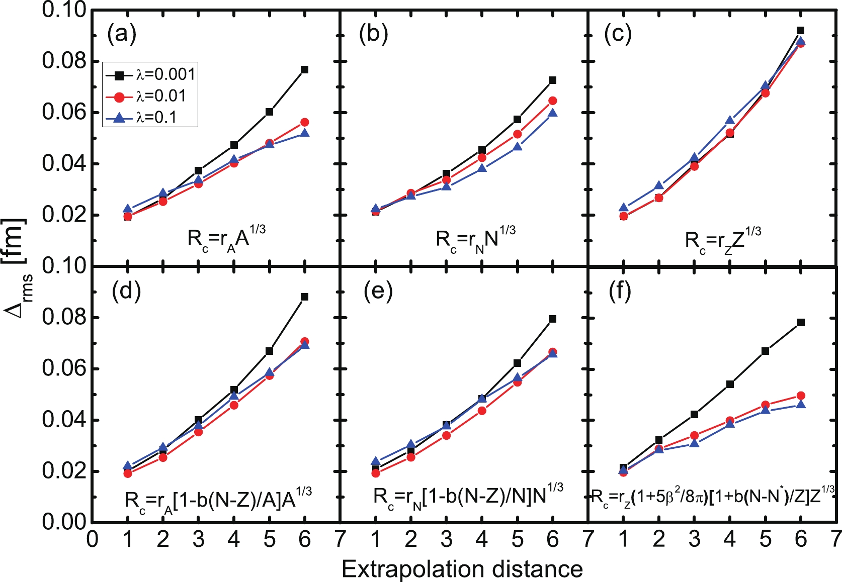
Figure 5. (color online) Effect of the ridge penalty term λ on the extrapolation power.
Very recently, the charge radii of several very exotic K and Ca isotopes have been observed [14, 15, 17]. Figure 6 shows the comparison between the experimental and calculated root-mean-square nuclear charge radii without (upper panels) and with (lower panels) KRR corrections for Ca and K isotopes. It can be seen that the calculated results by these six formulae without KRR corrections deviate a lot from the experimental data. After the KRR corrections being considered, all these six formulae can reproduce the data in "CR2013" quite well. However, for the "new" data observed by later experiments, the calculations become quite different. For the Ca isotopes [Fig. 6(c)], the
$ N^{1/3} $ and$ A^{1/3} $ formulae reproduce the data not very well, while other formulae reproduce the data at the same level. For the K isotopes [Fig. 6(d)], all the formulae can reproduce the data for the proton-rich side, while the$ A^{1/3} $ formula and the$ Z^{1/3} $ formula with isospin dependence can reproduce the data better for the neutron-rich side. It is also interesting to see that only the$ Z^{1/3} $ formulae with isospin dependence can reproduce the slight staggering in the K isotopes. This may be due to the deformation effect considered in this formula. Therefore, it can be seen that although KRR method is a powerful machine learning method, a microscopic model which can provide a better description of the nuclear charge radius is still needed. Note that a Bayesian neural network has also been applied to study the nuclear charge radii for the Ca and K isotopes recently [53].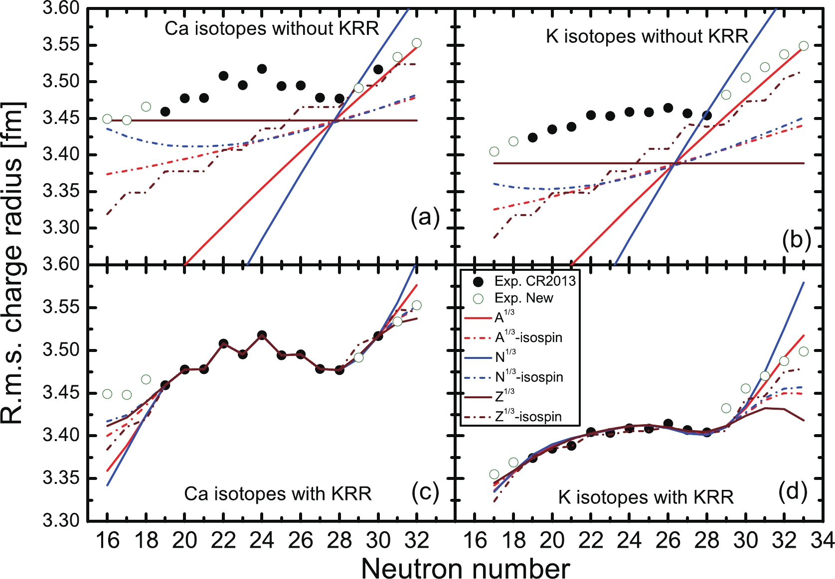
Figure 6. (color online) Comparison between experimental and calculated root-mean-square nuclear charge radii without (upper panels) and with (lower panels) KRR corrections for Ca and K isotopes. The experimental data taken from Ref. [13] (denoted as "CR2013") are shown by black solid circles, and the new data taken from Refs. [14, 15, 17] (denoted as "New") are shown by olive open circles.
-
The kernel ridge regression (KRR) method was adopted to improve the description of the nuclear charge radius by several phenomenological formulae. The widely used
$ A^{1/3} $ ,$ N^{1/3} $ and$ Z^{1/3} $ formulae, and their improved versions that include the isospin dependence, were adopted as examples. First, 884 experimental data with proton number$ Z \geq 8 $ and neutron number$ N \geq 8 $ were adopted for the least-square fitting with Levenberg–Marquardt method to obtain new parameters in these six phenomenological nuclear charge radius formulae. The root-mean-square deviations were reduced when these new parameters were adopted. Then the radius for each nucleus was predicted with the KRR network, which was trained with the deviations between experimental and calculated nuclear charge radii. For each formula, the resultant root-mean-square deviations was reduced to about 0.017 fm after considering the modification of the KRR method. The extrapolation ability of the KRR method for the neutron-rich region was examined carefully and compared with the radial basis function method. It was found that, compared with the RBF method, the improved nuclear charge radius formulae from the KRR method can avoid the risk of overfitting, and have a good extrapolation ability. The influence of the ridge penalty term on the extrapolation ability of the KRR method was analyzed. The charge radii of several recently observed K and Ca isotopes were also analyzed. -
The authors are grateful to X. H. Wu and P. W. Zhao for fruitful discussions.
Improved phenomenological nuclear charge radius formulae with kernel ridge regression
- Received Date: 2022-02-09
- Available Online: 2022-07-15
Abstract: The kernel ridge regression (KRR) method with a Gaussian kernel is used to improve the description of the nuclear charge radius by several phenomenological formulae. The widely used


 DownLoad: