


 Abstract
 HTML
HTML Reference
 Related
 PDF
PDF


-
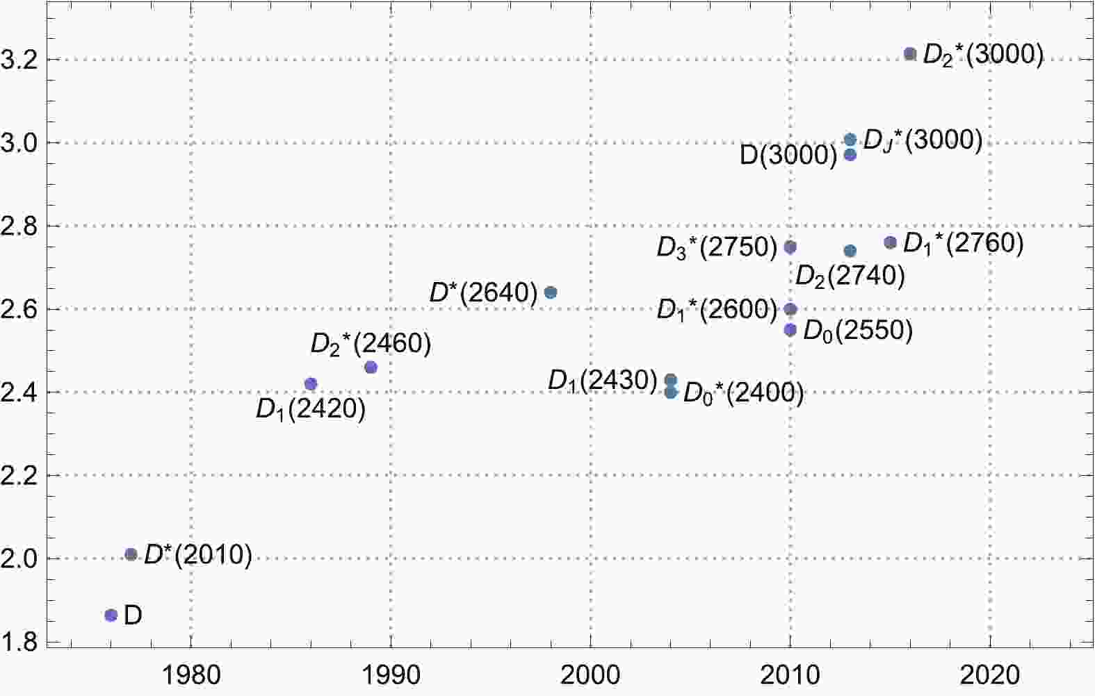
After the observations of
$ J/\psi $ in 1974 [1, 2], the crucial test of the notion of the charm quark is the existence of charmed mesons near 2 GeV, as indicated in Ref. [3]. Many experimental attempts have been made in various processes, and an increasing number of charmed mesons have been observed. In the following, we present a short review of the discovery history of charmed mesons.● The lowest S wave charmed mesons. The first charmed meson,
$ D^{0} $ , was observed after two years of the observation of$ J/\psi $ in the$ K^\pm \pi^\mp $ and$ K^\pm \pi^\mp \pi^\pm \pi^\mp $ invariant mass spectra produced by$ e^{+}e^{-} $ annihilation at the center-of-mass energies between 3.90 and 4.60 GeV [4], and soon after, its charged partner$ D^{\pm} $ was discovered in similar processes [5]. In 1977, another charmed meson,$ D^\ast $ , was observed in the$ e^{+}e^{-} $ annihilation process [6], which has been identified as a$ 1^{3}S_{1} $ charmed meson. Subsequently, the lowest S wave charmed mesons were fully established.● The lowest P wave charmed mesons. For P wave charmed mesons, the
$ J^P=1^+ $ state in the spin triplet can mix with the one in the spin singlet. In the heavy quark limit, one physical$ 1^+ $ state dominantly couples with$ D^\ast \pi $ via S wave, while another one dominantly couples with$ D^\ast \pi $ via D wave. In this case, the former$ D_1 $ should be much broader than the latter one. On the experimental side, the first P wave charmed meson,$ D_{1}(2420) $ , was observed in 1986 by the ARGUS collaboration at the DORIS II$ e^{+}e^{-} $ storage ring at DESY [7]. The mass and width were measured to be$ 2420\pm 6 $ and$ 70 \pm 21 $ MeV, respectively [7]. The angular momentum analysis indicated that the$ J^P $ quantum numbers of this state should be$ 1^{+} $ [7], which implies that$ D_1(2420) $ should be a P wave charmed meson. After the discovery of$ D_{1}(2420) $ , it has been further confirmed in other measurements [8–14]. The second observed P wave charmed meson is$ D_2(2460) $ , which was observed in the$ D^{+}\pi^{-} $ invariant mass spectrum by the E691 experiment at Fermilab [8]. The resonance parameters were observed to be$ m=2459 \pm 3 $ MeV and$ \Gamma=20 \pm 10 \pm 5 $ MeV, and its spin-parity was determined as$ J^{P}=2^{+} $ .The broader
$ D_1 $ state,$ D_{1}(2430) $ , with a mass$ 2427\pm 26 \pm 20 \pm 15 $ MeV and a width$ 384^{+107}_{-75} \pm 24 \pm 70 $ MeV was detected by the Belle Collaboration in 2004 [15]. In addition to$ D_1(2430) $ , another broad state$ D_{0}^{*}(2400) $ was observed in the$ D \pi $ invariant mass spectrum of$ B \to D \pi \pi $ process, which can be categorized as the last lowest P wave charmed meson with$ J^P=0^+ $ . The measure mass and width are$ 2308 \pm 17 \pm 15 \pm 28 $ and$ 276 \pm 21\pm 63 $ MeV, respectively. Subsequently, all the lowest P wave charmed mesons have been observed.●
$ D_0(2550) $ and$ D_1^\ast (2600) $ as$ 2S $ charmed meson candidates. In 2010, the BABAR Collaboration performed an analysis of the$ D^+ \pi^- $ ,$ D^0 \pi^+ $ , and$ D^\ast \pi^- $ system in the inclusive$ e^ +e^- \to c\bar{c} $ interaction to search for new excited charmed mesons, and four new states were observed, which are$ D_0(2550) $ ,$ D_1^\ast (2600) $ ,$ D_3(2750) $ , and$ D_1^\ast(2760) $ [12]. The mass and width of$ D_0(2550) $ were measured to be$ 2539.4\pm4.5\pm6.8 $ and$ 130 \pm 12 \pm 13 $ MeV, respectively, and the$ J^P $ quantum numbers were determined to be$ 0^- $ , which indicates that$ D_0(2550) $ could be a good candidate of the$ D(2^1S_0) $ state. The estimations of the mass spectrum and decay properties in Refs. [16–18] supported the$ D(2^1S_0) $ assignment for$ D_0(2550) $ .For
$ D_1^\ast (2600) $ , the resonance parameters were measured to be$ m=2608.7 \pm 2.4 \pm 2.5 $ MeV and$ \Gamma = 93 \pm 6 \pm 13 $ MeV, whereas the helicity angle distributions indicated that its$ J^P $ quantum numbers were$ 1^- $ . An estimation in Ref. [19] indicated that the mass of$ D_1^{*}(2600) $ was very close to the predicted value for$ D(2^{3}S_{1}) $ . The investigations of strong decay behaviors in the heavy quark effective theory with the leading order approximations supported that$ D_1^\ast(2600) $ could be the first radial excitation of$ D^{*} $ . It is worth noting that the estimations in Refs. [18, 20–22] also identified$ D_1^{*}(2600) $ as a$ 2^{3}S_{1} $ charmed meson.●
$ D_3(2750) $ ,$ D_1^\ast (2760) $ , and$ D_2(2740) $ as D wave charmed meson candidates. As indicated in Ref. [12],$ D_1^\ast(2760) $ and$ D_3(2750) $ were observed in the invariant mass spectra of$ D \pi $ and$ D^\ast \pi $ , respectively, and their mass and widths differ by$ 2.6\; \sigma $ and$ 1.5\; \sigma $ , respectively. The Dalitz plot analysis of$ B^{0}\rightarrow \bar{D}^{0}\pi^{+}\pi^{-} $ performed by the LHCb collaboration [23] indicated that the spin-parity of$ D_3(2750) $ should be$ 3^- $ , which is a good candidate of the$ 1^3D_3 $ charmed meson. For$ D_1^\ast (2760) $ , the analysis by the LHCb collaboration indicated that its spin-parity should be$ 1^- $ . The estimations in the frame of relativistic quark model in Ref. [24] indicated that$ D_1^\ast (2760) $ could be a good candidate of the$ 1^{3}D_{1} $ charmed meson. By investigating the mass spectrum and decay properties of charmed mesons, the authors in Ref. [22] explained$ D_1^\ast (2760) $ as a mixed state of$ D(2^{3}S_{1}) $ and$ D(1^{3}D_{1}) $ .Similar to the P wave charmed mesons, the two physical charmed mesons with
$ J^P=2^- $ are mixtures of the spin singlet and triplet. The first$ 2^- $ charmed meson,$ D_{2}(2740) $ , was observed in the$ D^{*}\pi $ invariant mass spectrum of the inclusive reaction$ pp \to D\pi X $ by the LHCb collaboration in 2013 [13]. The mass and width were observed to be$ 2737.0\pm3.5\pm11.2 $ and$ 73.2\pm 13.4\pm 25.0 $ MeV, respectively. Further analysis of the helicity angle distributions of$ B^{-}\rightarrow D^{*+}\pi^{-}\pi^{-} $ indicates the spin-parity of$ D_2(2740) $ as$ 2^- $ [14], which implies that$ D_{2}(2740) $ should be a$ 1^3D_2 $ charmed meson.● Higher charmed mesons at approximately 3 GeV. In 2013, the LHCb Collaboration observed two new charmed mesons,
$ D_J(3000) $ and$ D^{*}_{J}(3000) $ , in the$ D^{*}\pi $ and$ D\pi $ invariant mass spectrum of the inclusive reactions$ pp\to D^{(\ast)} \pi X $ , respectively [13]. The resonance parameters of$ D_J(3000) $ are$ m=2971.8\pm8.7 $ MeV and$ \Gamma=188.1\pm44.8 $ MeV. The helicity angular distributions of$ D_J(3000) $ are compatible with unnatural parity. The mass and width of$ D^{*}_{J}(3000) $ are$ 3008.1\pm4.0 $ and$ 110.5\pm11.5 $ MeV, respectively [13]. Through further analysis of the$ D \pi $ invariant mass spectra of the exclusive process$ B^{-}\rightarrow D^{+}\pi^{-}\pi^{-} $ , the LHCb collaboration observed one more broad resonance in the$ D\pi $ invariant mass distribution above 3 GeV [25]. The resonance parameters were fitted to be$ M=3214\pm29\pm49 $ MeV and$ \Gamma=186\pm38\pm34 $ MeV, and the Dalitz plot analysis indicated that its spin-parity was$ 2^+ $ [25]. The measured resonance parameters of$ D_2^\ast (3000) $ were not consistent with those of$ D_J^\ast(3000) $ , which indicates that the origins of$ D_2^\ast(3000) $ and$ D_J^\ast(3000) $ should be different.Besides the
$ 1F $ charmed mesons, the masses of$ 2P $ and$ 3S $ charmed mesons were also predicted to be around 3 GeV [16]; thus, these states can be good candidates of$ 1F $ and$ 2P $ charmed mesons. In Ref. [20], the authors investigated the decay properties of$ D_J(3000) $ and$ D^{*}_{J}(3000) $ using the$ 3P_{0} $ model, and they concluded that$ D_J(3000) $ can be categorized as the first radial excitation of$ D_{1}(2430) $ , and$ D^{*}_{J}(3000) $ can be categorized as a$ D(1^{3}F_{2}) $ or$ 1^{3}F_{4} $ charmed meson. The estimation in Ref. [18] indicated that$ D^{*}_{J}(3000) $ can be assigned as$ 1^{3}F_{4} $ , but$ D_J(3000) $ was a good candidate of the$ D(3^{1}S_{0}) $ charmed meson.A sketch diagram of the charmed mesons discovery history is presented in Fig. 1, where we observe that most higher charmed mesons were observed in the past decade. With the high energy and high luminosity beams at the LHC and SuperKEKB, higher charmed mesons have been observed, which undoubtedly enrich the charmed meson spectrum. The investigations of their properties are crucial for us to properly categorize these newly observed charmed mesons. In addiiton to the strong decay process, the electromagnetic decays of the hadron are sensitive to its inner structure; thus, the radiative transitions can also probe the internal charge structure of mesons and be useful in determining the meson structure.
To investigate the radiative decay properties of charmed mesons, we employ the quark model to estimate the mass spectra and wave functions. In Ref. [16], Godfrey and Isgur proposed a relativistic quark model (GI model) with chromodynamics to describe the entire meson spectra. The GI model achieved significant success in describing the ground state of the meson spectra. However, the model failed to address the higher excited states owing to a simple linear confinement potential without including the unquenched effects, which are expected to be important for higher excited states [28]. In Ref. [29], we replaced the simple linear potential with the screened potential, which can, to a certain extent, reflect the unquenched effects in the higher excited charmed mesons. With the modified GI model [29], we observed that the mass spectra and strong decay properties of the higher charmed mesons can be better described than those with the GI model. In this study, we employ the modified GI model to investigate the radiative decay properties of charmed mesons.
This paper is organized as follows. After the introduction, we present a review of the quark model employed in the present estimation and the formulas for radiative decays. The numerical results and discussions are provided in Sec. III, and the final section presents a summary.
-
From the perspective of classical physics, the light quark in the heavy-light meson system moves very rapidly relative to the heavy quark. Therefore, the relativistic effect cannot be ignored for heavy-light meson systems. The GI model proposed nearly forty years ago can fully describe the ground state meson spectrum of the heavy-light meson system. The hamiltonian of the GI model can be expressed as
$ \tilde{H}=(p^{2}+m^{2}_{1})^{1/2}+(p^{2}+m^{2}_{2})^{1/2}+\tilde{V}_{\mathrm{eff}}({\boldsymbol{p}},{\boldsymbol{r}}), $

(1) where
$ \tilde{V}_{\mathrm{eff}}({\boldsymbol{p}},{\boldsymbol{r}})=\tilde{V}^{\mathrm{conf}}+\tilde{V}^{\mathrm{hyp}}+\tilde{V}^{\mathrm{SO}} $ is the effective confinement potential between the quark and anti-quark in a meson. In the non-relativistic approximation, the effective potential can be expressed as$ V_{\mathrm{eff}}(r)=V^{\mathrm{conf}}(r)+V^{\mathrm{hyp}}(r)+V^{\mathrm{SO}}(r), $

(2) The spin-independent term
$ \tilde{V}^{\mathrm{conf}} $ is primarily composed of two parts: A short-distance$ \gamma^{\mu}\otimes\gamma_{\mu} $ interaction of one-gluon-exchange and a long-distance$ 1\otimes1 $ linear confining interaction. The specific forms of these two interactions are a Coulomb potential and a long-range linear potential; subsequently,$ V^{\mathrm{conf}}_{ij}(r) $ is given by$ V^{\mathrm{conf}}_{ij}(r) = -\Bigg[\frac{3}{4}c+\frac{3}{4}br-\frac{\alpha_{s}(r)}{r}\Bigg]\Big({\boldsymbol{F}}_{i}\cdot{\boldsymbol{F}}_{j}\Big), $

(3) where i and j represent different quarks in the system. The concrete form of the color-hyperfine term is
$ \begin{aligned}[b] V^{\mathrm{hyp}}(r)=&-\frac{\alpha_{s}(r)}{m_{1}m_{2}}\Bigg[\frac{8\pi}{3}{\boldsymbol{S}}_{1}\cdot{\boldsymbol{S}}_{2}\delta^{3}({\boldsymbol{r}}) \\ & \times \frac{1}{r^{3}}\Bigg(\frac{3{\boldsymbol{S}}_{1}\cdot{\boldsymbol{rS}}_{2}\cdot r}{r^{2}}-{\boldsymbol{S}}_{1}\cdot{\boldsymbol{S}}_{2}\Bigg)\Bigg]\Big({\boldsymbol{F}}_{i}\cdot{\boldsymbol{F}}_{j}\Big). \end{aligned} $

(4) and the spin orbit term
$ V^{\mathrm{SO}} $ consists of two parts, and it is given by$ V^{\mathrm{SO}}_{ij}(r)=V^{\mathrm{SO(cm)}}_{ij}+V^{\mathrm{SO(tp)}}_{ij}, $

(5) where the former is the color-magnetic term, and the later is the Thomas-precession term. The concrete forms of these two terms are
$ V^{\mathrm{SO(cm)}}_{ij}(r)=-\frac{\alpha_{s}(r)}{r^{3}}\Bigg[\frac{1}{m_{i}}+\frac{1}{m_{j}}\Bigg]\Bigg[\frac{{\boldsymbol{S}}_{i}}{m_{i}}+\frac{{\boldsymbol{S}}_{j}}{m_{j}}\Bigg]\cdot{\boldsymbol{L}}\Big({\boldsymbol{F}}_{i}\cdot{\boldsymbol{F}}_{j}\Big), $

(6) $ V^{\mathrm{SO(tp)}}_{ij} (r) =-\frac{1}{2r}\frac{\partial V^{\mathrm{conf}}_{ij}}{\partial r}\Bigg[\frac{{\boldsymbol{S}}_{i}}{m^{2}_{i}}+\frac{{\boldsymbol{S}}_{j}}{m^{2}_{j}}\Bigg]\cdot{\boldsymbol{L}} , $

(7) where
$ {\boldsymbol{S}}_{1} $ and$ {\boldsymbol{S}}_{2} $ represent the spins of the quark and anti-quark, respectively, and$ {\boldsymbol{L}}={\boldsymbol{r}}\times{\boldsymbol{p}} $ is the orbital angular momentum. The value of$ {\boldsymbol{F}}_i \cdot {\boldsymbol{F}}_j $ is$ -4/3 $ in meson systems.The influence of the relativistic effect is considered from two aspects, i.e., the non-locality of the effective potential of the quark and antiquark interactions and the momentum dependences of the effective potential on momentum. For the first type of correction, we can introduce a smearing function, which is
$ \rho_{12}({\boldsymbol{r}}-{\boldsymbol{r'}})=\frac{\sigma^{3}_{12}}{\pi^{3/2}}\mathrm{exp}\big(-\sigma^{2}_{12}({\boldsymbol{r}}-{\boldsymbol{r'}})\big), $

(8) with
$ \sigma^{2}_{12}=\sigma^{2}_{0} \Bigg[\frac{1}{2}+\frac{1}{2}\left(\frac{4m_{1}m_{2}}{(m_{1}+m_{2})^{2}}\right)^{4}\Bigg]+s^{2}\left(\frac{2m_{1}m_{2}}{m_{1}+m_{2}}\right)^{2}. $

(9) The potentials of relativistic form is
$ \tilde{f_{12}}(r)=\int {\rm d}^{3}{\boldsymbol{r'}}\rho_{12}({\boldsymbol{r}}-{\boldsymbol{r'}})f(r'), $

(10) where
$ \tilde{f}(r) $ and$ f(r) $ represent the potentials in the relativistic and nonrelativistic forms, respectively.The second type of relativistic corrections is introducing the momentum dependences in the effective potentials. The corrected Coulomb potential is expressed as [16]:
$ \tilde{G}(r)\rightarrow \left[1+\frac{p^{2}}{E_{1}E_{2}}\right]^{1/2}\tilde{G}(r)\left[1+\frac{p^{2}}{E_{1}E_{2}}\right]^{1/2}. $

(11) The corrected forms of the tensor, contact, vector spin-orbit, and scalar spin-orbit potentials are expressed as follows:
$ \frac{\tilde{V}_{i}(r)}{m_{1}m_{2}}\rightarrow \left[1+\frac{p^{2}}{E_{1}E_{2}}\right]^{1/2+\epsilon_{i}}\frac{\tilde{V}_{i}(r)}{m_{1}m_{2}}\left[1+\frac{p^{2}}{E_{1}E_{2}}\right]^{1/2+\epsilon_{i}}. $

(12) The parameters
$ \epsilon_i $ are different for different effective potentials, which have been listed in Ref. [16]. -
The GI model is successful in describing the low-lying meson spectrum, but it has encountered problems in describing highly excited states. The predictions given by the GI model is considerably different from experimental measurements [30–34]. For example, the observed masses of
$ X(3872) $ ,$ D_{s0}^\ast (2317) $ , and$ D_{s1}(2460) $ are significantly lower than the expectations of the relativistic quark model [16, 35]. Further theoretical estimations indicated that the near-threshold effect of the coupling channel depresses the mass of the high excited-state [36–38]. From the perspective of the quark model, the coupling channel effects can be phenomenologically described by screening the color charges at a large distance, for example, a distance greater than 1 fm, by creating light quark-antiquark pairs. Estimations using the unquenched Lattice QCD [39–41] and holographic models [42] have confirmed the existence of the screening effects in hadrons.In literature, the screening effect in charmonia [28, 43], light unflavored mesons [44], and heavy light mesons [29, 45] have been investigated by flattening the linear confinement potential. In Ref. [28], the screening effect in charmonia was proposed to be described by replacing the linear confinement potential with a screened potential in the form
$ br\rightarrow V^{\mathrm{scr}}(r)=\frac{b(1-{\rm e}^{-\mu r})}{\mu}, $

(13) where the corrected potential behaves as a linear potential
$ br $ at the short distance and approaches a constant$ b/\mu $ at a long distance. Following the method in Ref. [16], we can transfer the non-relativistic effective potential to the relativistic form using$ \tilde{V}^{\mathrm{scr}}=\int {\rm d}^{3}{\boldsymbol{r'}}\rho_{12}({\boldsymbol{r}}-{\boldsymbol{r'}})\frac{b(1-{\rm e}^{-\mu r'})}{\mu}. $

(14) Note that the above screened potential scheme was also introduced to describe the heavy light meson families in Refs. [29, 45], where the mass spectrum and strong decay behaviors of excited charmed and charmed strange mesons can be well described. In this study, we adopt the same modified GI model as the one in Ref. [45] to estimate the mass spectrum and radiative decays of the charmed mesons. The estimated mass spectrum of charmed mesons are listed in Table 1. For comparison, we also list the spectrum predicted by the GI model and the experimental measurements [12, 35]. The table shows that the modified GI model can better describe the mass spectrum of charmed mesons.
States GI model [16] Modified GI model [45] PDG [12, 35] $ 1^{1}S_{0} $ 

1874 1861 $ 1864.84\pm0.07 $ 

$ 2^{1}S_{0} $ 

2583 2534 $ 2539.4\pm4.5\pm6.8 $ 

$ 3^{1}S_{0} $ 

3068 2976 $ 1^{3}S_{1} $ 

2038 2020 $ 2010.26\pm0.7 $ 

$ 2^{3}S_{1} $ 

2645 2593 $ 2608.7\pm2.4\pm2.5 $ 

$ 3^{3}S_{1} $ 

3111 3015 $ 1P_{1} $ 

2455 2424 $ 2421.4\pm0.6 $ 

$ 2P_{1} $ 

2933 2866 $ 1^{3}P_{0} $ 

2398 2365 $ 2318\pm29 $ 

$ 2^{3}P_{0} $ 

2932 2865 $ 1P_{1}^{ \prime } $ 

2467 2434 $ 2427\pm26\pm25 $ 

$ 2P_{1}^{ \prime } $ 

2952 2872 $ 1^{3}P_{2} $ 

2501 2468 $ 2464.3\pm1.6 $ 

$ 2^{3}P_{2} $ 

2957 2884 $ 1D_{2} $ 

2827 2775 $ 2D_{2} $ 

3225 3127 $ 1^{3}D_{1} $ 

2816 2762 $ 2^{3}D_{1} $ 

3231 3131 $ 1D_{2}^{ \prime } $ 

2834 2777 $ 2D_{2}^{ \prime } $ 

3235 3133 $ 1^{3}D_{3} $ 

2833 2779 $ 2^{3}D_{3} $ 

3226 3129 Table 1. Spectrum of the charm mesons in MeV. The theoretical predictions of the GI model; the experimental measurements are also presented for comparison.
-
With the wave function evaluated by the modified GI model, we can investigate the radiative decays of charmed mesons. The start point of the radiative decay is the quark-photon electromagnetic coupling at the tree level, which is
$ H_{em}=-\sum_{j}e_{j}\bar{\psi}_{j}\gamma^{j}_{\mu}A^{\mu}({\boldsymbol{k}},{\boldsymbol{r}})\psi_{j}, $

(15) where
$ {\psi}_{j} $ represents the j-th quark field in the charmed meson,$ e_{j} $ is the charge carried by the j-th constituent quark, and$ {\boldsymbol{k}} $ is the three momentum of the emitted photon.In the non-relativistic limit, the spinor
$ \bar{\psi} $ can be replaced by$ \psi^{\dagger} $ , while the$ \mathit{\boldsymbol{\gamma}} $ matrices become$ \mathit{\boldsymbol{\alpha}} $ matrices. In this case, the electromagnetic transitions operator can be expressed as [46–48]$ h_{e}\simeq\sum_{j}\left[e_{j}{\boldsymbol{r}}_{j}\cdot\mathit{\boldsymbol{\epsilon}}-\frac{e_{j}}{2m_{j}}\mathit{\boldsymbol{\sigma}}_{j}\cdot(\mathit{\boldsymbol{\epsilon}}\times{\boldsymbol{\hat{k}}})\right]{\rm e}^{-{\rm i}{\boldsymbol{k}}\cdot {\boldsymbol{r}}_{j}}, $

(16) where
$ m_{j} $ and$ {\boldsymbol{r}}_{j} $ are the mass and coordinate of the j-th constituent quark, respectively,$ \mathit{\boldsymbol{\sigma}}_{j} $ is the Pauli matrix, and$ {\bf{\epsilon}} $ is polarization vector of the photon. In the above transition operator, the first and second terms correspond to the electric and magnetic transitions, respectively.Considering the electromagnetic transitions between the initial state
$ |i\rangle $ and final state$ |f\rangle $ , the helicity amplitudes of the electric and magnetic transitions are$ \mathcal{A}^{E}_{\lambda}=- i\sqrt{\frac{\omega_{\gamma}}{2}}\big\langle f \big|\sum_{j}e_{j}{\boldsymbol{r}}_{j}\cdot\mathit{\boldsymbol{\epsilon}}{\rm e}^{-{\rm i}{\boldsymbol{k}}\cdot{\boldsymbol{r}}_{j}} \big| i \big\rangle, $

(17) $ \mathcal{A}^{M}_{\lambda}=+i\sqrt{\frac{\omega_{\gamma}}{2}}\big \langle f \big|\sum_{j}\frac{e_{j}}{2m_{j}}\mathit{\boldsymbol{\sigma}}_{j}\cdot(\mathit{\boldsymbol{\epsilon}}\times\mathit{\boldsymbol{\hat{k}}}){\rm e}^{-{\rm i}{\boldsymbol{k}}\cdot{\boldsymbol{r}}_{j}} \big| i \big \rangle, $

(18) where
$ \omega_{\gamma} $ is energy of the emitted photon.In the initial hadron stationary system, we can select the photon momentum
$ {\boldsymbol{k}} $ along the z axial direction, i.e.,$ {\boldsymbol{k}}=\{0,0,k\} $ , and polarization vector of the photon with the right-hand to be$ \mathit{\boldsymbol{\epsilon}}=-{1}/{\sqrt{2}}(1,i,0) $ . Considering the multipole expansion of$ {\rm e}^{-{\rm i}{\boldsymbol{k}}\cdot{\boldsymbol{r}}_{j}} $ , the helicity amplitudes in Eq. (18) can be expanded using amplitudes with a certain angular momentum l, which are [49, 50]$ \begin{aligned}[b] \mathcal{A}^{El}_{\lambda}=&\sqrt{\frac{\omega_{\gamma}}{2}}\big\langle J^{\prime}\lambda^{\prime} \big| \sum_{j}(-i)^{l}B_{l}e_{j}j_{l+1}(kr_{j})r_{j}Y_{l1}\big| J\lambda \big \rangle \\ & +\sqrt{\frac{\omega_{\gamma}}{2}} \big \langle J^{\prime}\lambda^{\prime} \big| \sum_{j}(-i)^{l}B_{l}e_{j}j_{l-1}(kr_{j})r_{j}Y_{l1}\big| J\lambda \big\rangle , \end{aligned} $

$ \begin{aligned}[b] \mathcal{A}^{Ml}_{\lambda}=&\sqrt{\frac{\omega_{\gamma}}{2}}\big\langle J^{\prime}\lambda^{\prime}\big|\sum_{j}(-i)^{l}C_{l}\frac{e_{j}}{2m_{j}}j_{l-1}(kr_{j}) \\ & \times[\sigma^+_{j}\otimes Y_{l-10}]^{l}_{1}\big|J\lambda\big \rangle \\ & +\sqrt{\frac{\omega_{\gamma}}{2}}\big \langle J^{\prime}\lambda^{\prime}\big|\sum_{j}(-i)^{l}C_{l}\frac{e_{j}}{2m_{j}}j_{l-1}(kr_{j}) \\ & \times[\sigma^+_{j}\otimes Y_{l-10}]^{l-1}_{1}\big|J\lambda\big \rangle, \end{aligned} $

(19) with
$ B_{l}=\sqrt{2\pi l(l+1)/(2l+1)} $ and$ C_{l}=i\sqrt{8\pi (2l-1)} $ .As indicated in Ref. [50], the high angular momentum contributions are negligible compared with the lowest order approximation with
$ l=1 $ . Thus, in the lowest order approximation, the electric transition widths is [51]$ \begin{aligned}[b] \Gamma^{E_1}=&\frac{4}{3}\alpha \Bigg(\frac{e_{1}m_{2}}{m_{1}+m_{2}}-\frac{e_{2}m_{1}}{m_{1}+m_{2}}\Bigg)^{2}\omega^{3}_{\gamma}\delta_{SS^{\prime}}\delta_{LL^{\prime}\pm1}\max\left(L,L^{\prime}\right) \\ &\times (2J^{\prime}+1)\begin{Bmatrix}L^{\prime} & J^{\prime} & S \\ J & L & 1\end{Bmatrix}^{2}\big\langle n^{\prime 2S^{\prime}+1}L^{\prime}_{J^{\prime}}\big|r\big|n^{2S+1}L_{J}\big\rangle^2, \end{aligned} $

(20) and the magnetic transition width is
$ \begin{aligned}[b] \Gamma^{M_1}=&\frac{\alpha}{3}\omega_{\gamma}^{3}\delta_{LL^{\prime}}\delta_{SS^{\prime}\pm1}\frac{2J^{\prime}+1}{2L+1}\big\langle n^{\prime2S^{\prime}+1}L^{\prime}_{J^{\prime}}\big|\frac{e_{1}}{m_{1}}j_{0}\Bigg(\omega_{\gamma}\frac{m_{2}r}{m_{1}+m_{2}}\Bigg) \\ & -\frac{e_{2}}{m_{2}}j_{0}\Bigg(\omega_{\gamma}\frac{m_{1}r}{m_{1}+m_{2}}\Bigg)\big|n^{2S+1}L_{J}\big\rangle^2, \end{aligned} $

(21) where
$ \left \langle n^{\prime 2S^{\prime }+1}L^{\prime }_{J^{\prime }}\right| $ and$ \left \langle n^{2S+1}L_{J}\right| $ represent the space function of the final and initial states, respectively, which are estimated using the modified GI model,$ e_{1}(m_1) $ and$ e_{2}(m_2) $ represent the charge (mass) of the charm and anti-light quark, respectively, and α is the fine structure constant. -
For the heavy-light system, the
$ ^1L_\ell $ and$ ^3L_\ell $ states have the same$ J^P $ quantum numbers; thus, the physical states are the mixtures of these two states. In this study, we have$ \begin{array}{*{20}{l}} \left( \begin{array}{c} |nL_1 \rangle\\ |nL_1^\prime\rangle \end{array} \right)= \left( \begin{array}{cc} \cos\theta_{L} &\sin \theta_L\\ -\sin\theta_{L} &\cos \theta_L\\ \end{array} \right) \left( \begin{array}{c} |n^1L_1 \rangle\\ |n^3L_1\rangle \end{array} \right), \end{array} $

(22) where
$ L=P $ and D correspond to P and D wave charmed mesons, respectively. In the heavy quark limit, the mixing angle$ \theta_{P} $ and$ \theta_{D} $ are estimated to be$ -54.7^{\circ} $ and$ -50.8^{\circ} $ , respectively. In addition to the above mixing, the tensor term in the Hamiltonian can result in the mixing between the states with an angular momentum difference of two, such as the mixing between$ ^3S_1 $ and$ ^3D_1 $ . As indicated in Refs. [29, 45], this type of mixing is rather small; thus, in the following estimations, such mixing is neglected. -
As indicated in Eq. (20), the
$ E_1 $ transitions occur between the states with the same spins but an angular momenta difference of one. In Tables 2–5, we present the electric transitions of$ S\to P \gamma $ ,$ P\to S\gamma $ ,$ P\to D \gamma $ , and$ D\to P\gamma $ , where S, P, and D refer to the$ S- $ ,$ P- $ , and$ D- $ wave charmed mesons, respectively. It is worth noting that in the quark model, the masses of the up and down quarks usually have the same value, and then, the estimated mass spectra and wave functions for the charged and neutral charmed mesons are identical. Thus, for the$ E_1 $ transition as shown in Eq. (20), the only difference for the charged and neutral charmed mesons is the charge of the involved quarks. Setting$ m_c=1628 $ MeV and$ m_u=m_d=220 $ MeV [16], we determine the E1 transition for the neutral states to be approximately 9.7 times the corresponding one for the charged states.Initial state Final state Width ( $c\bar{u}$ /

$c\bar{d}$ )

Present Ref. [52] Ref. [51] $2^{1}S_{0}$ 

$1P_{1}$ 

11.5/1.2 44.6/4.61 $1P^{ \prime }_{1}$ 

26.2/2.7 77.8/4.7 7.83/0.809 $2^{3}S_{1}$ 

$1^{3}P_{0}$ 

21.6/2.2 66/3.8 23.6/2.43 $1P_{1}$ 

21.5/2.2 40.7/2.3 8.25/0.852 $1P^{ \prime }_{1}$ 

11.8/1.2 29.8/3.08 $1^{3}P_{2}$ 

35.8/3.7 163/9.4 45.5/4.70 $3^{1}S_{0}$ 

$1P_{1}$ 

11.4/1.2 39.3/4.06 $1P^{ \prime }_{1}$ 

23.2/2.4 8.64/0.89 $2P_{1}$ 

22.0/2.3 138/14.3 $2P^{ \prime }_{1}$ 

68.1/7.0 18.7/1.93 $3^{3}S_{1}$ 

$1^{3}P_{0}$ 

2.4/0.3 2.60/0.269 $1P_{1}$ 

$\sim0$ /

$\sim0$ 

$\sim0$ /

$\sim0$ 

$1P^{ \prime }_{1}$ 

$\sim0$ /

$\sim0$ 

0.32/ $\sim0$ 

$1^{3}P_{2}$ 

40.7/4.2 65.7/6.79 $2^{3}P_{0}$ 

18.6/1.9 24.4/2.52 $2P_{1}$ 

30.8/3.2 24.9/2.57 $2P^{ \prime }_{1}$ 

21.3/2.2 41.7/4.30 $2^{3}P_{2}$ 

84.9/8.8 131/13.5 Initial state Final state Width ( $c\bar{u}$ /

$c\bar{d}$ )

Present Ref. [51] $1^{3}D_{1}$ 

$1^{3}P_{0}$ 

488.9/50.5 521/53.8 $1P_{1}$ 

177.0/18.3 55.9/5.78 $1P^{ \prime }_{1}$ 

174.2/18.0 222/22.9 $1^{3}P_{2}$ 

14.4/1.5 15.9/1.64 $1D_{2}$ 

$1P_{1}$ 

21.0/2.2 642/66.4 $1P^{ \prime }_{1}$ 

579.4/59.9 12.2/1.26 $1^{3}P_{2}$ 

88.3/9.1 55.4/5.72 $1D^{ \prime }_{2}$ 

$1P_{1}$ 

571.4/59.0 64.7/6.69 $1P^{ \prime }_{1}$ 

77.6/8.0 640/66.1 $1^{3}P_{2}$ 

60.9/6.3 116/11.9 $1^{3}D_{3}$ 

$1^{3}P_{2}$ 

625.0/64.6 686/70.9 $2^{3}D_{1}$ 

$1^{3}P_{0}$ 

8.2/0.9 $1P^{ \prime }_{1}$ 

0.7/0.1 $1P_{1}$ 

1.5/0.1 $1^{3}P_{2}$ 

3.6/0.4 $2^{3}P_{0}$ 

314.9/32.5 $2P^{ \prime }_{1}$ 

76.6/7.9 $2P_{1}$ 

172.2/17.8 $2^{3}P_{2}$ 

15.5/1.6 $2D_{2}$ 

$1P_{1}$ 

0.7/0.1 $1P^{ \prime }_{1}$ 

5.9/1.6 $1^{3}P_{2}$ 

4.9/0.5 $2P_{1}$ 

15.2/1.6 $2P^{ \prime }_{1}$ 

435.8/45.0 $2^{3}P_{2}$ 

75.1/7.7 $2D^{ \prime }_{2}$ 

$1P_{1}$ 

6.1/0.6 $1P^{ \prime }_{1}$ 

0.3/ $\sim0$ 

$1^{3}P_{2}$ 

5.1/0.5 $2^{3}P_{0}$ 

77.6/8.0 $2P_{1}$ 

391.8/40.5 $2P^{ \prime }_{1}$ 

57.3/5.9 $2^{3}P_{2}$ 

52.9/5.4 $2^{3}D_{3}$ 

$1^{3}P_{2}$ 

1.1/0.1 $2^{3}P_{2}$ 

442.4/45.7 Table 5. Same as Table 2 but for
$ D\to P\gamma $ processes.●
$ S \to P\gamma $ processes. In Table 2, we present our estimations of the electric transition widths from S wave to P wave charmed mesons, where$ c\bar{u} $ and$ c\bar{d} $ refer to the neutral and charged charmed mesons, respectively. For comparison, we also present the results from Refs. [51, 52]. In Ref. [52], the wave functions were evaluated in a simple nonrelativistic quark model with a color Coulomb plus linear scalar confinement interaction with the addition of a Gaussian smeared contact hyperfine interaction term. For the$ 2S \to 1P \gamma $ processes, the results of Ref. [52] are several times larger than those of this study owing to the different model parameters. In Ref. [51], the radiative decays were investigated using the GI model. From the table, we observe that the radiative transition widths of the process involving$ P_{1}/P_1^{\prime} $ states are significantly different because of the different mixing angles used in the present estimations and Ref. [51], while the widths of other channels are very similar. The influence of mixing angle on the radiative decay process are discussed later. Moreover, the widths of$ D(2^{1}S_{0})^{0} $ and$ D^{*}(2^{3}S_{1})^{0} $ were measured to be$ 199\pm5\pm17 $ and$ 149\pm4\pm20 $ MeV, respectively [14], thus the branching ratios of$ 2S \to 1P \gamma $ processes are of the order$ 10^{-4} $ and$ 10^{-5} $ for neutral and charged charmed mesons, respectively.For
$ 3S $ states, our estimation indicates that the partial widths of$ 3S \to 1P \gamma $ processes are suppressed compared with those of$ 3S\to 2P \gamma $ processes because of the node effects. In particular, our estimations indicate that the widths of$ D^0(3^1S_0) \to D_1^{\prime 0}(2P^\prime_1) \gamma $ and$ D(3^3S_1)^0 \to D_2(2^3P_2)^{0} \gamma $ are approximately 100 keV. In Ref. [45], the widths of$ D(3^1S_0) $ and$ D^{\ast}(3^3S_1) $ were approximately 100 MeV; thus, the branching ratios of$ D^0(3^1S_0) \to D_1^{\prime 0}(2P^\prime_1) \gamma $ and$ D^{\ast 0}(3^3S_1) \to D_2^0(2^3P_2) \gamma $ should be of the order of$ 10^{-3} $ , which may be detected by further measurements in the LHCb and Belle II experiments.●
$ P \to S\gamma $ processes. In Table 3, we present our estimations of the$ E_1 $ transition widths of$ P-S\gamma $ processes. The estimations in Refs. [51–54] are also presented for comparison. For$ 1^3P_0 \to 1^3S_{1} \gamma $ and$ 1^3P_2 \to 1^3S_1 \gamma $ processes, we observe that our results are almost the same as those in Ref. [51] since the modified relativistic quark model used in this study is similar to the GI model employed in Ref. [51]. For$ 1P_1/1P_1^\prime \to 1S \gamma $ , our estimation is slightly different from those in Ref. [51] owing to the different mixing angle$ \theta_{1P} $ used in the estimations.Initial state Final state Width ( $c\bar{u}$ /

$c\bar{d}$ )

Present Ref. [51] Ref. [52] Ref. [53] Ref. [54]a $1^{3}P_{0}$ 

$1^{3}S_{1}$ 

275.4/28.5 288/30 304/17 $115\pm54/ <2.8$ 

$1P_{1}$ 

$1^{1}S_{0}$ 

254.9/26.4 640/66 349.3/19.7 $245\pm18$ 

$1^{3}S_{1}$ 

290.2/30.0 82.8/8.6 $60\pm5$ 

$1P^{ \prime }_{1}$ 

$1^{1}S_{0}$ 

533.1/55.1 156/16.1 $14\pm6/<3.3$ 

$1^{3}S_{1}$ 

155.4/16.1 386/39.9 549.5/30.9 $93\pm44/<2.3$ 

$1^{3}P_{2}$ 

$1^{3}S_{1}$ 

577.4/59.7 592/61.2 895/51 $2^{3}P_{0}$ 

$1^{3}S_{1}$ 

63.7/6.6 76.4/7.90 $2^{3}S_{1}$ 

362.6/37.5 427/44.1 $2P_{1}$ 

$1^{1}S_{0}$ 

7.8/0.8 14.1/1.46 $1^{3}S_{1}$ 

7.4/0.8 3.70/0.382 $2^{1}S_{0}$ 

180.9/18.7 384/39.6 $2^{3}S_{1}$ 

275.5/28.5 88.9/9.19 $2P^{ \prime }_{1}$ 

$1^{1}S_{0}$ 

14.9/1.5 4.88/0.505 $1^{3}S_{1}$ 

3.5/0.4 12.9/1.34 $2^{1}S_{0}$ 

315.2/32.6 162/16.7 $2^{3}S_{1}$ 

117.0/12.1 396/40.9 $2^{3}P_{2}$ 

$1^{3}S_{1}$ 

14.0/1.4 10.9/1.12 $2^{3}S_{1}$ 

366.9/37.9 425/43.9 a Only the $E_1$ transitions between the neutral charmed meson were estimated.

Table 3. Same as Table 2 but for
$ P-S\gamma $ processes. The theoretical estimation in Refs. [51–54] are also presented for comparison. The mixing angles of Refs. [51] and [52] are$ \theta_{1P}=-25.68^{\circ}/\theta_{2P}=-29.39^{\circ} $ and$ \theta_{1P}=-26^{\circ} $ , respectively, while the mixing angle is ignored in Ref. [53].To explore the influence of the mixing angle on the electrical transition width, we present the mixing angle dependences of the radiative decay widths of the process
$ D_1^0(1P_1) \to D^{(\ast) 0} \gamma $ and$ D_1^{\prime 0}(1P_1^\prime) \to D^{(\ast) 0} \gamma $ in Figs. 2 and 3, respectively. For the electric transition processes, the initial and final states should have the same spin; thus, the widths of$ D^{0}_{1}(1P_{1}) \to D^{*0}\gamma $ and$ D^{\prime 0}_{1}(1P^{\prime}_{1}) \to D^{0}\gamma $ should be proportional to$ \sin^2 \theta_{1P} $ , while the widths of$ D^{\prime 0}_{1}(1P^\prime_{1}) \to D^{*0}\gamma $ and$ D^{ 0}_{1}(1P_{1}) \to D^{0}\gamma $ are proportional to$ \cos^2 \theta_{1P} $ . In the figures, we also show the different mixing angles used in this study and Ref. [51], which are$ \theta_{1P}=-54.7^{\circ} $ and$ \theta_{1P}=-25.68^{\circ} $ , respectively. As indicated in the figures, the widths of the processes of$ D^{0 (\prime)}_{1}(1P^{(\prime)}_{1}) \to D^{(\ast)0}\gamma $ calculated in this study are similar to those in Ref. [51] when we use the same mixing angle$ \theta_{1P} $ 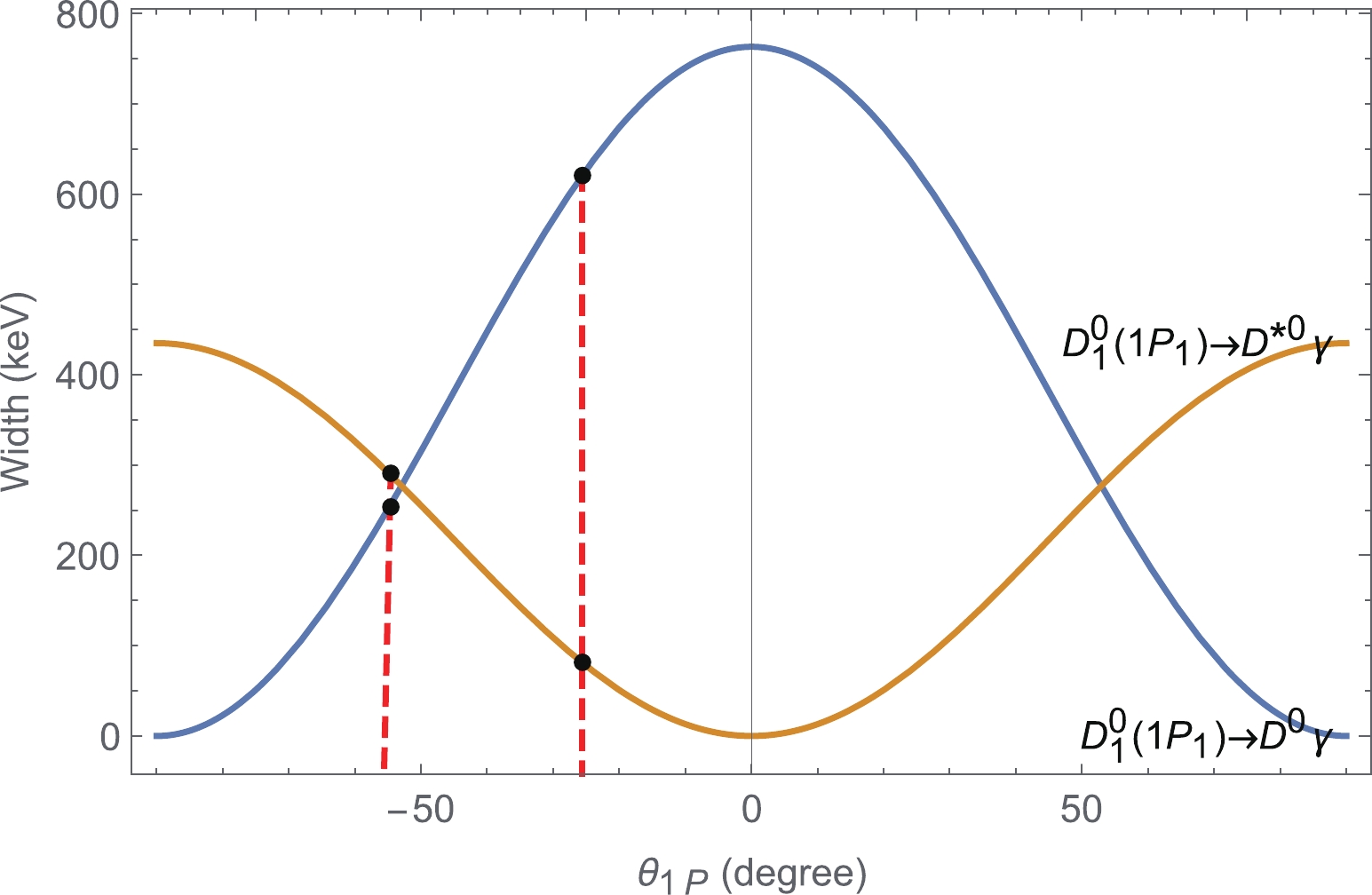
Figure 2. (color online) Width of the process
$ D^{0}_{1}(1P_{1}) \to $ $ D^{*0}/D^{0}\gamma $ depending on the mixing angle$ \theta_{1P}. $ 
Figure 3. (color online) Same as Fig. 2 but for
$ D^{\prime 0}_{1}(1P^{\prime}_{1}) \to $ $ D^{*0}/D^{0}\gamma. $ Our estimations are also comparable to those in Ref. [52], where the wave functions are estimated in a non-relativistic quark model. However, the estimations based on the heavy quark effective theory in Refs. [53, 54] are several times smaller than the potential model estimation in this study and Refs. [51, 52]. For
$ 1P \to 1S \gamma $ processes, the present estimations indicate the widths of all the possible processes are greater than 100 keV. The PDG average of the widths of$ D_0(1^3P_0) $ ,$ D_1(1P_1) $ ,$ D_1(1P_1^\prime) $ , and$ D_2(1^3P_2) $ are$ 229 \pm 16 $ ,$ 31.3 \pm 1.9 $ ,$ 314\pm 29 $ , and$ 47.3 \pm 0.8 $ MeV, respectively. Thus, for$ D_1(1P_1) $ and$ D_2(1^3P_2) $ , the branching ratios of the$ E_1 $ transitions are of the order of$ 10^{-3} \sim 10^{-2} $ , which are sufficiently large to be detected.Similar to the
$ S \to P \gamma $ process, our estimation also indicates that$ 2P \to 1S \gamma $ processes are suppressed compared with the$ 2P \to 2S \gamma $ process owing to node effects. In particular, we observe that the widths of$ D_0^0(2^3P_0) \to D^{\ast 0}(2^3S_1) \gamma $ ,$ D_1^0(2P_1) \to D^0(2^1S_0) \gamma $ ,$ D_1^0(2P_1) \to D^{\ast 0}(2^3S_1) \gamma $ ,$ D_1^{\prime 0}(2P_1^\prime) \to D^0(2^1S_0) \gamma $ ,$ D_1^{\prime 0}(2P_1^\prime) \to D^{\ast 0}(2^3S_1) \gamma $ , and$ D_2^0(2^3P_2) \to D^{\ast 0}(2^3S_1) \gamma $ are larger than 100 keV. Our estimations in Ref. [45] indicated the widths of$ 2P $ charmed mesons to be approximately 100 MeV; thus, the branching ratios of the above processes should be of the order of$ 10^{-3} $ .●
$ P \to D\gamma $ processes. As shown in Table 4, our estimations indicate that the$ E_1 $ transition widths of$ 2P \to 1D \gamma $ are rather small, which are similar to those in Ref. [51]. In this study, only the widths of$ D_0^0(2^3P_0) \to D_1^0(1^3D_1) \gamma $ ,$ D_1^0(2P_1) \to D_2^{\prime 0}(1D^\prime_2) \gamma $ ,$ D_1^{\prime 0}(2P_1^\prime) \to D_2^{0}(1D_2) \gamma $ , and$ D_2^0(2^3P_2) \to D_3^0(1^3D_3) \gamma $ are several tens keV. However, the widths of$ 2P $ charmed mesons are approximately 100 MeV; thus, the branching ratio of these channel should be at most of the order of$ 10^{-4} $ . The widths of the other seven channels are even smaller. Thus, it is difficult to detect the$ 2P \to 1D \gamma $ processes experimentally.Initial state Final state Width ( $c\bar{u}$ /

$c\bar{d}$ )

Present Ref. [51] $2^{3}P_{0}$ 

$1^{3}D_{1}$ 

19.8/2.0 30.5/3.15 $2P_{1}$ 

$1^{3}D_{1}$ 

2.5/0.3 1.26/0.13 $1D_{2}$ 

0.9/0.1 25.1/2.59 $1D^{ \prime }_{2}$ 

18.8/1.9 0.476/ $\sim0$ 

$2P^{ \prime }_{1}$ 

$1^{3}D_{1}$ 

3.1/0.3 9.30/0.961 $1D_{2}$ 

14.0/1.4 0.385/ $\sim0$ 

$1D^{ \prime }_{2}$ 

1.4/0.1 26.7/2.76 $2^{3}P_{2}$ 

$1^{3}D_{1}$ 

0.2/ $\sim 0$ 

0.36/ $\sim0$ 

$1D_{2}$ 

2.2/0.2 2.02/0.208 $1D^{ \prime }_{2}$ 

1.2/0.1 2.47/0.255 $1^{3}D_{3}$ 

23.8/2.5 34.2/3.53 ●
$ D\to P\gamma $ processes. Our estimations of the widths of$ D\to P \gamma $ are listed in Table 5. By comparing our estimations with the results in Ref. [51], we observe that the transition widths are very similar, except for the processes with mixing states, such as$ 1P_1 $ and$ 1P_1^\prime $ . As indicated in Fig. 2 and Fig. 3, such discrepancies result from the different mixing angles adopted in the calculations. For$ 1D \to P \gamma $ processes, our estimations indicate that the widths of$ D_1^0(1^3D_1) \to D_0^0(1^3P_0) \gamma $ ,$ D_2^0(1D_2) \to D_1^{\prime 0}(1P^\prime_1) \gamma $ ,$ D_2^{\prime 0}(1D_2^\prime) \to D_1^{0}(1P_1) \gamma $ , and$ D_3^0(1D_3) \to D_2^0(1^3P_2) \gamma $ are greater than 400 keV. The experimental measurement and theoretical estimations in Ref. [45] indicated that the widths of$ D_1(1^3D_1) $ ,$ D_2(1D_2) $ and$ D_2^\prime (1D_2^\prime) $ are approximately 100 MeV; thus, the branching ratios of$ D_1^0(1^3D_1) \to D_0^0(1^3P_0) \gamma $ ,$ D_2^0(1D_2) \to D_1^{\prime 0}(1P_1^\prime) \gamma $ , and$ D_2^{\prime 0}(1D_2^\prime) \to D_1^{0}(1P_1) \gamma $ should be of the order of$ 10^{-3} $ . The width of$ D_3(1D_3) $ is estimated to be 18.3 MeV, which indicates that the branching ratio of$ D_3^0(1D_3) \to D_2^0(1^3P_2) \gamma $ is approximately$ 3\% $ , which should be observable experimentally.For the electric decays of
$ 2D $ states, we observe that the widths of$ 2D \to 1P \gamma $ are smaller than the corresponding one of$ 2D \to 2P \gamma $ , which is similar to that of the electric decays of$ 3S $ and$ 2P $ states. For the$ 2D\to 2P \gamma $ process, our estimations show that the widths of the$ D_1^0(2^3D_1) \to D_0^0(2^3P_0) \gamma $ ,$ D_2^0(2D_2) \to D_1^{\prime 0}(2P_1^\prime) \gamma $ ,$ D_2^{\prime 0}(2D_2^\prime)\to D_1^{0}(2P_1) \gamma $ , and$ D_3^0(2^3D_3) \to D_2^0(2^3P_2) \gamma $ processes are 314.8, 435.8, 391.8, and 442.4 keV, respectively. As indicated in Ref. [45], the widths of$ D(2^3D_1) $ and$ D(2D_2) $ are approximately 100 MeV, while the widths of$ D_2^\prime (2D_2^\prime) $ and$ D_3(2^3D_3) $ are approximately 30 MeV; thus, we observe that the branching ratios of$ D_1^0 (2^3D_1)\to D_0^0(2^3P_0) \gamma $ and$ D_2^0(2D_2) \to D_1^{\prime 0}(2P_1^\prime) \gamma $ are of the order of$ 10^{-3} $ , while the branching ratios of$ D_2^{\prime 0}(2D_2^\prime) \to D_1^{0}(2P_1) \gamma $ and$ D_3^0(2^3D_3) \to D_2^0(2^3P_2) \gamma $ are of the order of$ 10^{-2} $ , which should be accessible in further experiments. -
As indicated in Eq. (21), the
$ M_1 $ transitions occur between the states with the same angular but different spin. Our estimations of the$ M_1 $ transition for$ S\to S \gamma $ ,$ P\to P \gamma $ and$ D\to D\gamma $ are listed in Tables 6–8, respectively.Initial state Final state Width ( $c\bar{u}$ /

$c\bar{d}$ )

Present Ref. [51] Ref. [52] Ref. [53] $1^{3}S_{1}$ 

$1^{1}S_{0}$ 

97.0/9.9 106/10.2 32/1.8 43.6/1.1 $2^{1}S_{0}$ 

$1^{3}S_{1}$ 

0.4/4.3 $\sim0$ /5.80

$2^{3}S_{1}$ 

$1^{1}S_{0}$ 

526.4/87.0 600/100 $2^{1}S_{0}$ 

5.4/0.5 6.26/0.641 $3^{1}S_{0}$ 

$1^{3}S_{1}$ 

0.8/3.6 $\sim0$ /6.27

$2^{3}S_{1}$ 

24.6/13.2 44.5/22.4 $3^{3}S_{1}$ 

$1^{1}S_{0}$ 

547.9/97.2 663/119 $2^{1}S_{0}$ 

189.7/68.0 257/48.2 $3^{1}S_{0}$ 

1.5/0.1 2.03/0.208 Initial state Final state Width ( $c\bar{u}$ /

$c\bar{d}$ )

$1D_{2}$ 

$1^{3}D_{1}$ 

$\sim0$ /

$\sim0$ 

$1D^{ \prime }_{2}$ 

$1^{3}D_{1}$ 

0.1/ $\sim0$ 

$1D_{2}$ 

$\sim0$ /

$\sim0$ 

$1^{3}D_{3}$ 

$1D_{2}$ 

$\sim0$ /

$\sim0$ 

$2^{3}D_{1}$ 

$1D_{2}$ 

2.3 /1.2 $1D^{ \prime }_{2}$ 

3.0/1.5 $2D_{2}$ 

$\sim0$ /

$\sim0$ 

$2D_{2}$ 

$1^{3}D_{1}$ 

12.1/2.1 $1D_{2}$ 

21.1/5.0 $1D^{ \prime }_{2}$ 

0.3/0.1 $1^{3}D_{3}$ 

4.8/1.9 $2D^{ \prime }_{2}$ 

$1^{3}D_{1}$ 

20.0/3.4 $1D_{2}$ 

1.9/0.3 $1D^{ \prime }_{2}$ 

21.5/5.0 $2^{3}D_{1}$ 

$\sim0$ /

$\sim0$ 

$2D_{2}$ 

$\sim0$ /

$\sim0$ 

$2^{3}D_{3}$ 

$1D_{2}$ 

17.5/3.1 $2D_{2}$ 

$\sim0$ /

$\sim0$ 

Table 8. Same as Table 6 but for
$ D\to D\gamma $ processes.●
$ S\to S \gamma $ processes. In Table 6, we present our estimations to the$ M_1 $ transitions between two S wave charmed mesons. For comparison, we also present the estimations from the GI model [51], nonrelativistic quark model [52], and heavy quark effective theory [53]. For$ D^\ast \to D \gamma $ , we observe that the widths of$ D^{\ast 0} \to D^0 \gamma $ and$ D^{\ast +} \to D^+ \gamma $ are approximately 97 and 9.9 keV, respectively, which are consistent with the estimation in GI model and several times larger than the one in non-relativistic quark model [52] and heavy quark effective theory [53].On the experimental side, the width of
$ D^{\ast+} $ is$ 83.4 \pm 1.8 $ keV, and the branching ratio of$ D^{\ast +} \to D^{+} \gamma $ is measured to be$ (1.6 \pm 0.4)\% $ ; thus, the measured width of$ D^{\ast +} \to D^{+} \gamma $ is$ 1.33 \pm 0.33 $ keV, which is several times smaller than the estimation in this study. For$ D^{\ast 0} \to D^0 \gamma $ , the branching ratio has been well determined, which is$ (35.3\pm 0.9)\% $ , but only the upper limit of the width of$ D^{\ast 0} $ has been measured, which is 2.1 MeV. Thus, the upper limit of width of$ D^{\ast 0} \to D^0 \gamma $ is approximately 740 keV, which is significantly larger than the present estimation. Furthermore, we can estimate the partial widths of$ D^{\ast 0} \to D^0 \gamma $ using the relative fraction of$ D^{\ast 0} \to D^0 \gamma $ and$ D^{\ast 0} \to D^0 \pi^0 $ . The PDG average of the branching ratio of$ D^{\ast 0} \to D^0 \pi^0 $ is$ (64.7 \pm 0.9 )\% $ , which is approximately$ 1.83 $ times that of$ D^{\ast 0} \to D^0 \gamma^0 $ , while the partial widths of$ D^{\ast 0} \to D^0 \pi^0 $ can be deduced from that of$ D^{\ast +} \to D^{+} \pi^0 $ by considering the isospin symmetry [55, 56]. Subsequently, the width of$ D^{\ast 0} \to D^0\gamma $ is estimated to be approximately 15 keV, which is also several times smaller than the present estimation and the results of the GI model.Note that the magnetic transition width in Eq. (21) is sensitive to the quark mass. Using the process
$ D^\ast \to D \gamma $ as an example, we can expand the spherical Bessel function$ j_0(x) \simeq 1 -x^2/6 +\mathcal{O}(x^4) $ ; thus, in the leading order approximation, the magnetic transition width is proportional to$ (e_1m_2-e_2m_1)^2/(m_1^2m_2^2) $ . In the present modified GI model and the GI model, the mass of the light quark is 220 MeV, while in the non-relativistic quark model, the mass of the light quark is often set to be 330 MeV. A smaller light quark mass usually results in larger magnetic transition widths. In Fig. 4, we present the widths of the process$ D^{+*} \to D^{+}\gamma $ depending on the light quark mass, in which we observe that the width will be approximately 2 keV when we use$ m_d=0.33 $ GeV, which is several times smaller than that of$ m_d=0.22 $ GeV and consistent with the experimental measurements.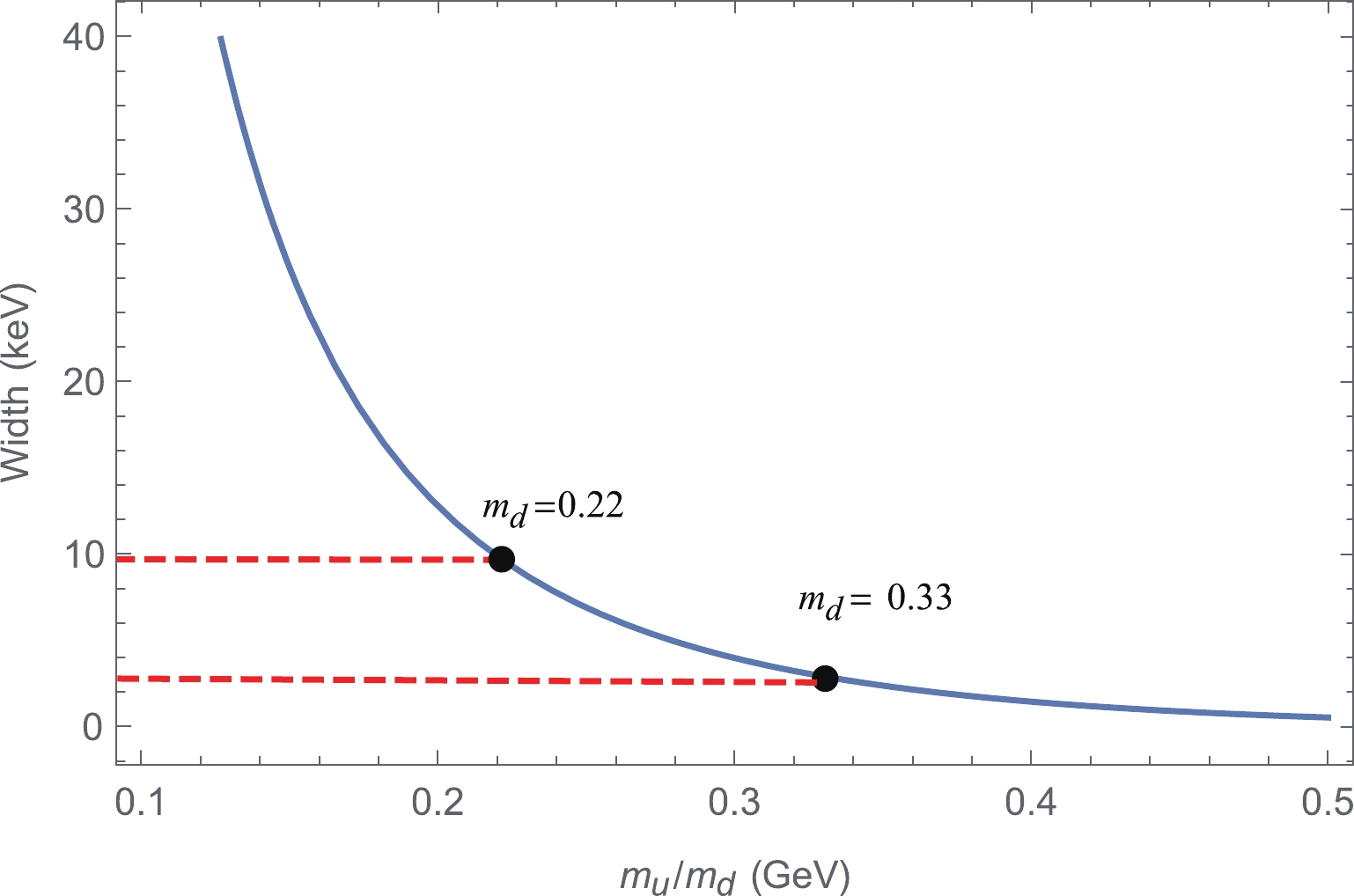
Figure 4. (color online) Width of
$ D^{+*} \to D^{+}\gamma $ depending on the light quark moass.Our estimations indicate that the widths of
$ D^{\ast 0} (2^3S_1) \to D^{0} \gamma $ and$ D^{\ast 0} (3^3S_1) \to D^{0} \gamma $ are greater than 500 keV, which are also consistent with the estimations in the GI model [51]. The PDG average of the widths of$ D_1^\ast(2600) $ is$ 141 \pm 23 $ MeV; thus, the branching ratio of$ D^{\ast 0} (2^3S_1) \to D^{0} \gamma $ is approximately$ 3.7 \pm 10^{-3} $ . The width of$ D^{\ast 0} (3^3S_1) $ was estimated to be 80 MeV in the modified GI model [45]; thus, the branching ratio of$ D^{\ast 0} (3^3S_1) \to D^{0} \gamma $ is approximately$ 6.8 \times 10^{-3} $ .●
$ P \to P \gamma $ processes. As shown in Table 7, the widths of most of the$ P\to P \gamma $ processes are significantly small. In particular, the widths of the$ 1P \to 1P \gamma $ process are several keV or less than 1 keV. The widths of the$ 2P \to 1P \gamma $ process vary from several keV to several tens keV. For$ 2P \to 2P \gamma $ processes, the widths are very small and most of them are close to 0.Initial state Final state Width ( $c\bar{u}$ /

$c\bar{d}$ )

$1P_{1}$ 

$1^{3}P_{0}$ 

1.4/0.1 $1P^{ \prime }_{1}$ 

$1P_{1}$ 

$\sim0$ /

$\sim0$ 

$1^{3}P_{2}$ 

$1P_{1}$ 

1.4/0.1 $1P^{ \prime }_{1}$ 

0.5/0.1 $2^{3}P_{0}$ 

$1P_{1}$ 

4.2/2.6 $1P^{ \prime }_{1}$ 

1.8/1.2 $2P_{1}$ 

$1^{3}P_{0}$ 

30.8/5.4 $1P_{1}$ 

33.5/8.2 $1P^{ \prime }_{1}$ 

6.0/1.2 $1^{3}P_{2}$ 

3.7/2.9 $2^{3}P_{0}$ 

$\sim0$ /

$\sim0$ 

$2P^{ \prime }_{1}$ 

$1^{3}P_{0}$ 

17.6/3.1 $1P_{1}$ 

7.3/1.4 $1P^{ \prime }_{1}$ 

34.9/8.5 $1^{3}P_{2}$ 

0.6/0.4 $2^{3}P_{0}$ 

$\sim0$ /

$\sim0$ 

$2P_{1}$ 

$\sim0$ /

$\sim0$ 

$2^{3}P_{2}$ 

$1P_{1}$ 

37.6/6.5 $1P^{ \prime }_{1}$ 

78.5/13.6 $2P_{1}$ 

0.2/ $\sim0$ 

$2P^{ \prime }_{1}$ 

$\sim0$ /

$\sim0$ 

Table 7. Same as Table 6 but for
$ P\to P\gamma $ processes.●
$ D \to D \gamma $ processes. In Table 8, we present our estimations of the widths of the$ D\to D \gamma $ process. As for$ 1D \to 1D \gamma $ and$ 2D\to 2D \gamma $ processes, the widths are very small and most of them are less than 0.1 keV. As for$ 2D\to 1D \gamma $ process, the widths are estimated from several keV to several tens keV. The widths of$ 2D\to 1D \gamma $ are slightly higher than those of$ 1D \to 1D \gamma $ and$ 2D\to 2D \gamma $ processes, but the branching ratios of these channels should at most be of the order of$ 10^{-4} $ . -
Over the past two decades, an increasing number of charmed mesons have been observed experimentally, which makes the charmed meson spectrum abundant. However, categorizing these newly observed charmed mesons is a significant challenge for theorists. As one of the most successful QCD inspired quark models, the GI model can describe the low lying mesons adequately but fails for higher excited states owing to the coupled channel effects. In Refs. [29, 45], we introduced a screened potential in the GI model to substitute for the coupled channels effects, and in this modified GI model, the higher excited charmed mesons, including the mass spectra and strong decays, can be better described than those with the GI model. Similar to the strong decays, the radiative transitions can also probe the internal charge structure of mesons and be useful in determining meson structure; thus, in this study, we extend our estimations from Ref. [29, 45] to investigate the radiative decays of the charmed mesons.
By using the wave function obtained from modified GI model, we estimate the radiative transitions between the
$ mS $ ,$ nP $ , and$ nD $ charmed mesons ($ m=\{1,2,3\}, \; n= \{1,2\} $ ) in this study. Our estimations indicate that the branching ratios of some processes, including$ D_2^0(1^3P_2) \to D^{\ast 0 }(1^3S_1) \gamma $ ,$ D_3^0(1D_3) \to D_2^0(1^3P_2) \gamma $ ,$ D_2^{\prime 0}(2D_2^\prime) \to D_1^{0}(2P_1) \gamma, $ $ D_3^0(2^3D_3) \to D_2^0(2^3P_2) \gamma $ , and$ D^{\ast 0}(1^3S_1) \to D^0(1^1S_0) \gamma $ , are of the order of$ 10^{-2} $ , which should be sizable to be detected experimentally. Moreover, the branching ratios of some channels, for example,$ D_1^0(1P_1) \to D^0(1^1S_0) \gamma $ ,$ D^0(3^1S_0) \to D_1^{\prime 0}(2P_{1}^\prime) \gamma $ , and$ D^0 (3^3S_1) \to D_2^0(2^3P_2) \gamma $ are estimated to be approximately$ 10^{-3} $ , which may also be accessible with the accumulation of data in future experiments.
Radiative decays of charmed mesons in a modified relativistic quark model
- Received Date: 2022-01-17
- Available Online: 2022-07-15
Abstract: In this study, we perform systematic estimations of the radiative decays of the charmed mesons in a modified relativistic quark model. Our estimations indicate that the branching ratios of the processes of


 DownLoad: