


 Abstract
 HTML
HTML Reference
 Related
 PDF
PDF


-
The present Hubble constant value can be measured in several ways, e.g., by the ΛCDM model with CMB measurement fixing its parameters at a relatively early universe, or by the distance ladder method at a relatively late universe. The discrepancy between the values of these different methods is known as the
$ H_0 $ tension problem.In the late 1990s, the use of Type Ia supernovae as standard candles led to the discovery that the expansion of the universe is accelerating. Large-scale observations indicate a cosmological acceleration phase that occurs at a late time [1]. Hence, several attempts have been proposed to describe the cosmic accelerated scenario. In general, there are two types of interpretations for this cosmic phase: i) postulating an exotic form of energy with negative pressure commonly called dark energy or ii) modifying the laws of gravity. Numerous models have been proposed based on these two branches; however, it is difficult to determine the correct one owing to the degeneracies in the parameter space. Nevertheless, the ΛCDM model with six parameters could excellently fit almost all observational data, and has been set as the standard model of cosmology [2]. By assuming a flat space in the ΛCDM model, the final full-mission Planck measurements of the cosmic microwave background (CMB) anisotropies have deduced a value for the Hubble constant
$ {{H}_{0}} = \left(67.27\pm 0.60 \right)\;{\rm km/s/Mpc} $ . This is compatible with many earlier and recent estimates of$ H_0 $ . In contrast, multiple local expansion rate measurements find slightly higher$ H_0 $ values and slightly larger error bars. In addition, the latest value from the Supernovae and$ H_0 $ for the Dark Energy Equation of State (S$ H_0 $ ES) project, together with GAIA DR2 parallaxes, is$ {{H}_{0}} = \left(73.52\pm 1.62 \right)\;{\rm km/s/ $ $ Mpc} $ , which has a more than$ 3\sigma $ tension with the Planck CMB data [3]. This tension is one of the most intriguing problems in modern cosmology. There have been several attempts to solve the problem, such as introducing new physics beyond the standard ΛCDM cosmological model. The non-zero spatial curvature may be a choice solution to the$ H_0 $ tension problem. Observing that the Friedmann equation$ {{\dot{a}}^{2}}+K = \dfrac{8\pi G}{3}\rho {{a}^{2}} $ in the ΛCDM model with spatial curvature can be written as$ \begin{equation} 1-\frac{1}{\Omega } = \frac{3K}{8\pi G\rho {{a}^{2}}} \end{equation}, $

(1) where
$ \Omega = \dfrac{\rho }{{{\rho }_{c}}} = \dfrac{8\pi G\rho }{3}{{\left(\dfrac{a}{{\dot{a}}} \right)}^{2}} $ is cosmic density, one can find$ \dfrac{3K}{8\pi G\rho {{a}^{2}}}\propto {{a}^{2}} $ in the radiation dominated era while$ \dfrac{3K}{8\pi G\rho {{a}^{2}}}\propto a $ can be found in the matter-dominated era for$ \rho {{a}^{3}} = {\rm con}st $ . In other words, the absolute value of$ 1-\dfrac{1}{\Omega } $ should grow all the time from the early universe until now if$ K\ne 0 $ , because the cosmic scale factor is growing all the time. From the Planck period until now,$ a\left(t \right) $ increased by dozens of magnitudes, followed by the value of$ 1-\dfrac{1}{\Omega } $ , which also increased by dozens of magnitudes. Currently, the deviation of Ω to 1 is observed to be a magnitude of up to 1, followed by the current value of$ 1-\dfrac{1}{\Omega } $ , which should also be a magnitude of 1. Based on existing conclusions, we can get the cosmological density of the Planck period$ {{\Omega }_{p}} = 1\pm {{10}^{-N}} $ , where N is a constant more than dozens. It suggests that at the end of the Planck period, the critical and cosmic mass densities were the same in several significant numbers, and the two physical quantities were not exactly equal. Otherwise, after the long evolution, there is a universe without the present spatial quasi-flatness. The non-zero spatial curvature encounters the problem of fine-tuning somehow in the inflation scenario. However it is still sensible to figure out whether the present distance observations prefer a non-zero spatial curvature or not. Although the current cosmological observations strongly favor a spatially flat Universe, e.g., the combined Planck 2018 cosmic microwave background (CMB) and baryon acoustic oscillation measurements, which suggest that$ {{\Omega }_{K}} = 0.001\pm 0.002 $ [1], these constraints are based on the pre-assumption of a specific cosmological model (e.g., the standard ΛCDM model). Because of the strong degeneracy between spatial curvature and the equation of state of dark energy [4], it is rather difficult to constrain the two quantities simultaneously. In general, dark energy is assumed to be a cosmological constant for the estimation of curvature, or conversely, the Universe is assumed to be flat in a dark energy analysis. Indeed, if the density of dark energy is allowed to vary freely with time, constraints on the geometry of the Universe may not only become less stringent, but may even depend on the properties that dark energy was previously assumed to have [5]. However, a simple flatness assumption may result in an incorrect reconstruction of the dark energy equation of state, even if the real curvature is very small, and a cosmological constant assumption may lead to confusion between ΛCDM and a dynamical dark energy model [6]. Moreover, the tension between the most recent SneIa data and spatial flat assumption in the ΛCDM model [7] may eventually support a spatial non-flat universe [8]. It has been pointed out that the Planck 2018 CMB spectra prefer a positive spatial curvature at more than 99% confidence level (CL) [9, 10]. The combined analysis of Planck CMB anisotropy and luminosity distant data simultaneously excludes a flat universe and cosmological constant at 99% CL [11].The motivation behind the choice of non-flat cosmology is that, as conventionally believed, an early inflationary phase leads to an almost flat universe, although not exactly with a perfectly zero spatial curvature. This is not necessary if the number of e-foldings is not significantly large [12]. It is still possible that there is a contribution to the Friedmann equations from the spatial curvature when studying late-time universe, though substantially smaller than other energy components according to observations. Recent observations have complicated this problem by suggesting that the deceleration factors of the expansion of the universe change over time, and that the universe went from decelerating to accelerated expansion approximately 6 billion years ago.
In the ΛCDM model, the cosmological constant can be viewed from the perspective of vacuum energy density, which is responsible for the accelerated expansion of the universe. Considering the large scale Lorentz violation, the large-scale torsion distribution caused by the Lorentz violation effect combined with the vacuum energy density is responsible for the accelerating expansion [13]. Therefore, we can introduce the effective cosmological constant, which is responsible for the accelerating expansion of the universe. Using the evolution of matter density
$ {{\Omega }_{M}} $ and initial conditions, one can constrain the bare cosmological constant to a desirable range. The implications of the large scale Lorentz violation model with non-vanishing spatial curvature under these constrains will be discussed in this paper. -
The large scale Lorentz violation gravitation model with zero spatial curvature is discussed in Ref. [13]. The general FRW metric, including the open and closed spatial geometry, is expressed as
$ \begin{aligned}[b] {\rm d}{{s}^{2}} = {\rm d}{{t}^{2}}-{{a}^{2}}\left( t \right)\left( {\rm d}{{r}^{2}}/\left( 1-K{{r}^{2}} \right)\right.\left.+{{r}^{2}}{\rm d}{{\theta }^{2}}+{{r}^{2}}{\rm d}{{\theta }^{2}}+{{r}^{2}}{{\rm sin}^{2}}\theta {\rm d}{{\varphi }^{2}} \right). \end{aligned} $

(2) The equations of motion for the gravitational field equation is
$ \begin{equation} {{\tilde{G}}^{a}}_{\ \ b} = {{\tilde{R}}^{a}}_{\ \ b}-1/2\tilde{R}{{\delta }^{a}}_{b} = 8\pi G/{{c}^{4}}{{\left( {{T}_{M}}+{{T}_{\Lambda }} \right)}^{a}}_{b}, \end{equation} $

(3) in which
$ {{\tilde{G}}^{a}}_{\ \ b} $ ,$ {{\tilde{R}}^{a}}_{\ \ b} $ , and$ \tilde{R} $ denote the Einstein tensor, Ricci curvature tensor, and Ricci curvature scalar of the spacetime with Levi-Civita connection, respectively.$ {{T}_{\Lambda }} $ represents the energy-momentum tensor of the dark partner contributed by the contortion tensor, which is responsible for the accelerated expansion of the universe,$ {{\left[{{T}_{\Lambda }} \right]}^{a}}_{b} = {\rm diag}\left({{\rho }_{\Lambda }},-{{p}_{\Lambda }}, $ $ -{{p}_{\Lambda }},-{{p}_{\Lambda }} \right) $ . The dark partner energy density$ {{\rho }_{\Lambda }} $ and pressure$ {{p}_{\Lambda }} $ are expressed as$ \begin{equation} {{\rho }_{\Lambda }} = -\frac{{{c}^{4}}}{8\pi G}\left( 3{{\mathcal K}^{2}}+6{\mathcal K}\frac{{\dot{a}}}{a}-{{\Lambda }_{0}} \right) \end{equation} $

(4) and
$ \begin{equation} {{p}_{\Lambda }} = \frac{{{c}^{4}}}{8\pi G}\left( {{\mathcal K}^{2}}+4{\mathcal K}\frac{{\dot{a}}}{a}+2\dot{\mathcal K}-{{\Lambda }_{0}} \right) \;, \end{equation} $

(5) where
$ {\mathcal K}\left(t \right) = K_{11}^{0} = K_{22}^{0} = K_{33}^{0} $ represents the non-zero components of the contortion tensor and$ {{\Lambda }_{0}} $ is the bare cosmological constant, the geometrical contribution by vacuum energy density. The modified Friedmann equations in geometrical unit$ \dfrac{{{c}^{4}}}{8\pi G} = 1 $ can be expressed as$ \begin{equation} {{\left( \frac{{\dot{a}}}{a} \right)}^{2}}{\rm+}2\frac{{\dot{a}}}{a}{\mathcal K}+{{\mathcal K}^{2}}+\frac{K}{{{a}^{2}}} = \frac{1}{3}\left( \rho {\rm+}{{\Lambda }_{0}} \right) \end{equation} $

(6) and
$ \begin{equation} \ddot{a} = -\frac{a}{2}\left( p+\frac{1}{3}\rho \right){\rm+}\frac{1}{3}a{{\Lambda }_{0}}-\frac{\rm d}{{\rm d}t}\left( a{\mathcal K} \right)\;. \end{equation} $

(7) As a reference, the Friedmann equations for ΛCDM model are
$ \begin{equation} {{\left( \frac{{\dot{a}}}{a} \right)}^{2}} = \frac{1}{3}\left( \rho +\Lambda \right) \end{equation} $

(8) and
$ \begin{equation} \ddot{a} = -\frac{a}{2}\left( p+\frac{\rho }{3} \right)+\frac{1}{3}a\Lambda \;. \end{equation} $

(9) This research attempts to explore the implications of the large scale Lorentz violation model with non-vanishing spatial curvature. It should be noted that the model lacks the evolution of
$ {\mathcal K}\left(t \right) $ , and the set of Eqs. (6) and (7) is not closed. As discussed in [13–15], the scales of the Lorentz violation region during the quantum gravity dominating era are stretched out beyond the horizon by inflation, and the region with sub-scale may reenter the horizon during normal expansion. In principle, the specific quantum gravity and inflation models are required to provide the prediction on the evolution of$ {\mathcal K}\left(t \right) $ . However, the evolution of$ {\mathcal K}\left(t \right) $ can be approximated by employing the ΛCDM model or assuming an equation of state satisfied by the dark partner phenomenologically. One can add an independent equation from the set of Friedmann equations of the ΛCDM model to close the set of modified Friedmann equations with two choices, as in [14, 15]. The third approximation comes from adding the equation of state for the dark partner to the modified Friedmann equations set. The three types of approximation can be given as follows [14, 15].Notice that (6) and (7) can be combined into one equation when the equation of state
$ p = w\rho $ is assumed,$ \begin{aligned}[b] \frac{{\ddot{a}}}{a}&+\frac{3w+1}{2}{{\left(\frac{{\dot{a}}}{a}\right)}^{2}}+\left(3w+2 \right)\frac{{\dot{a}}}{a}\mathcal K+\dot{\mathcal K}+\frac{3w+1}{2}{{\mathcal K}^{2}}\\&+\frac{3w+1}{2}\frac{\mathcal K}{{{a}^{2}}}-\frac{w+1}{2}{{\Lambda }_{0}} = 0\;, \end{aligned} $

(10) with a reference equation
$ \begin{equation} \frac{{\ddot{a}}}{a} = -\frac{3w+1}{2}{{\left( \frac{{\dot{a}}}{a} \right)}^{2}}{\rm+}\frac{w+1}{2}\Lambda \end{equation} $

(11) in the ΛCDM model. The first kind of approximation named Case A is
$ \begin{equation} \frac{1}{3}a{{\Lambda }_{0}}-\frac{1}{3}a\Lambda = \frac{\rm d}{{\rm d}t}\left( a{\mathcal K} \right), \end{equation} $

(12) obtained by combining (7) and (9). The second type named Case B is
$ \begin{equation} \left( 3w+2 \right)\frac{{\dot{a}}}{a}{\mathcal K}{\rm+}\dot{\mathcal K}{\rm+}\frac{3w+1}{2}{{\mathcal K}^{2}}{\rm+}\frac{3w+1}{2}\frac{K}{{{a}^{2}}}{\rm+}\frac{w+1}{2}\left( \Lambda -{{\Lambda }_{0}} \right){\rm{ = 0}}, \end{equation} $

(13) obtained by combining (10) and (11), while the third one named Case C is
$ \begin{equation} \left( 4{\rm+}6{{w}_{0}} \right)\frac{{\dot{a}}}{a}{\mathcal K}{\rm+}\left( 1+3{{w}_{0}} \right){{\mathcal K}^{2}}+2\dot{\mathcal K} = \left( {{w}_{0}}+1 \right){{\Lambda }_{0}}, \end{equation} $

(14) with the assumption that the equation of state for dark partner is
$ \begin{equation} {{p}_{\Lambda }} = {{w}_{0}}{{\rho }_{\Lambda }} \;. \end{equation} $

(15) The Friedmann equation of the ΛCDM model can be expressed as
$ \begin{equation} \Lambda = 3{{\left( \frac{{\dot{a}}}{a} \right)}^{2}}-\rho\;. \end{equation} $

(16) Similarly, the modified Friedmann equation of the large scale Lorentz violation model can be expressed as
$ \begin{equation} {{\Lambda }_{0}}-{\rm{6}}{\mathcal K}\frac{{\dot{a}}}{a}-3{{\mathcal K}^{2}}-3\frac{K}{{{a}^{2}}} = 3{{\left( \frac{{\dot{a}}}{a} \right)}^{2}}-\rho. \end{equation} $

(17) Comparing (16) and (17), it is not only the bare cosmological constant
$ {{\Lambda }_{0}} $ that contributes to the accelerated expansion of the universe in the large scale Lorentz violation model, but also the contribution from$ {\mathcal K}\left(t \right) $ , whose total contribution can define the effective cosmological constant$ \begin{equation} {{\Lambda }_{\rm eff}}\equiv {{\Lambda }_{0}}-6H{\mathcal K}-3{{\mathcal K}^{2}}-\frac{3K}{{{a}^{2}}}. \end{equation} $

(18) The initial value of
$ {\mathcal K}\left(t \right) $ , the contortion component value at present, can be obtained by the Friedmann equation of the ΛCDM model with two possible choices. The first type of initial value is$ \begin{equation} {\mathcal K}\left( {{t}_{0}} \right) = {{H}_{0}}\left\{ -1+\sqrt{1-\frac{K}{a_{0}^{2}H_{0}^{2}}-\frac{\Lambda }{3H_{0}^{2}}+\frac{{{\Lambda }_{0}}}{3H_{0}^{2}}} \right\}, \end{equation} $

(19) while the second one is
$ \begin{equation} {\mathcal K}\left( {{t}_{0}} \right) = {{H}_{0}}\left\{ -1-\sqrt{1-\frac{K}{a_{0}^{2}H_{0}^{2}}-\frac{\Lambda }{3H_{0}^{2}}+\frac{{{\Lambda }_{0}}}{3H_{0}^{2}}} \right\}. \end{equation} $

(20) To ensure the values of contortion components take real numbers, there should be a constrain condition satisfied by the bare cosmological constant, cosmological constant observed, and spatial curvature,
$ K/a_{0}^{2}+ \Lambda /3- $ $ {{\Lambda }_{0}}/3\le H_{0}^{2} $ , i.e.,$ \begin{equation} {{\Lambda }_{0}}\ge \Lambda {\rm+}\frac{{\rm{3}}K}{a_{0}^{2}}-3H_{0}^{2}. \end{equation} $

(21) For a specific large scale Lorentz violation model, the spatial curvature constant K, current cosmic scale factor
$ {{a}_{0}} $ , Hubble constant$ {{H}_{0}} $ , and bare cosmological constant$ {{\Lambda }_{0}} $ are the free input parameters given by observation or predicted by a more fundamental theory model. It can be defined that$ \begin{equation} {{\Lambda }_{\rm min}} = \Lambda {\rm+}\frac{{\rm{3}}K}{a_{0}^{2}}-3H_{0}^{2} \end{equation} $

(22) from condition (21), such that there is a minimum for the free input bare cosmological constant,
$ \Lambda _0 \ge \Lambda _{\rm min} $ , to facilitate a feasible evolution of the universe.Because the accelerated expansion occurs in the late stage of the cosmic evolution, we mainly concentrate on considering the matter-dominated era. In the case of
$ w = 0 $ , the evolution of the Hubble parameters and contortion can be obtained by the modified Friedmann equations (6), (7), and one of the three kind of approximations, (12), (13) and (14), with both the initial values of$ {\mathcal K}\left(t \right) $ in (19) and (20). The evolution of H versus time in different cases are presented in Figs. 1 and 2. Figure 1 shows that the behavior of the evolution of the Hubble parameter in Case C2 deviates rather significantly from other cases and the ΛCDM model. However, deviation among different models become small after the scale factor of the universe, a, becomes greater than 1. The evolutions of Case B and ΛCDM models tend to be identically the same globally.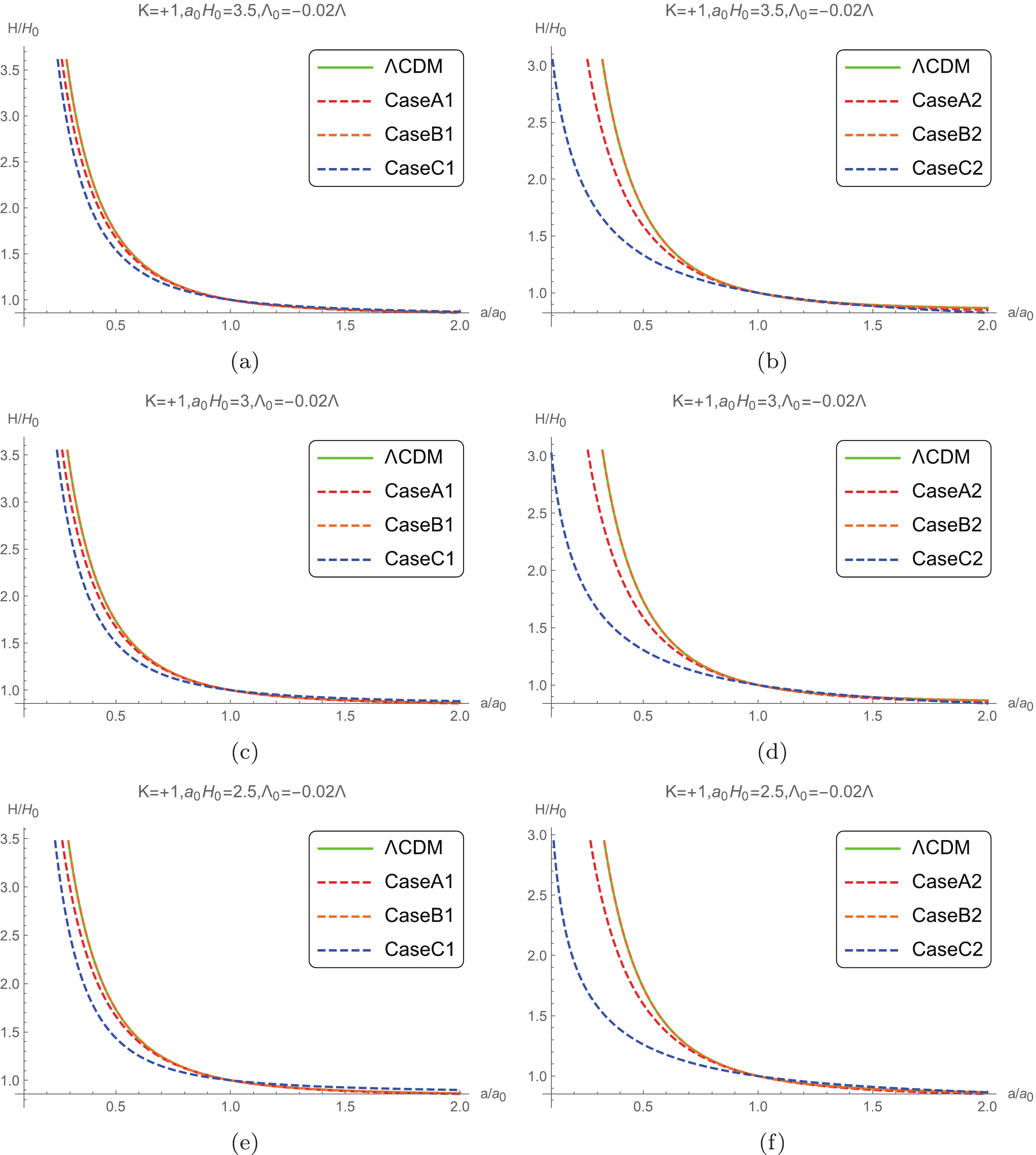
Figure 1. (color online) Hubble constant evolving with the scale factor when
$ K = +1,\;{{\Lambda }_{0}} = -0.02\Lambda $ .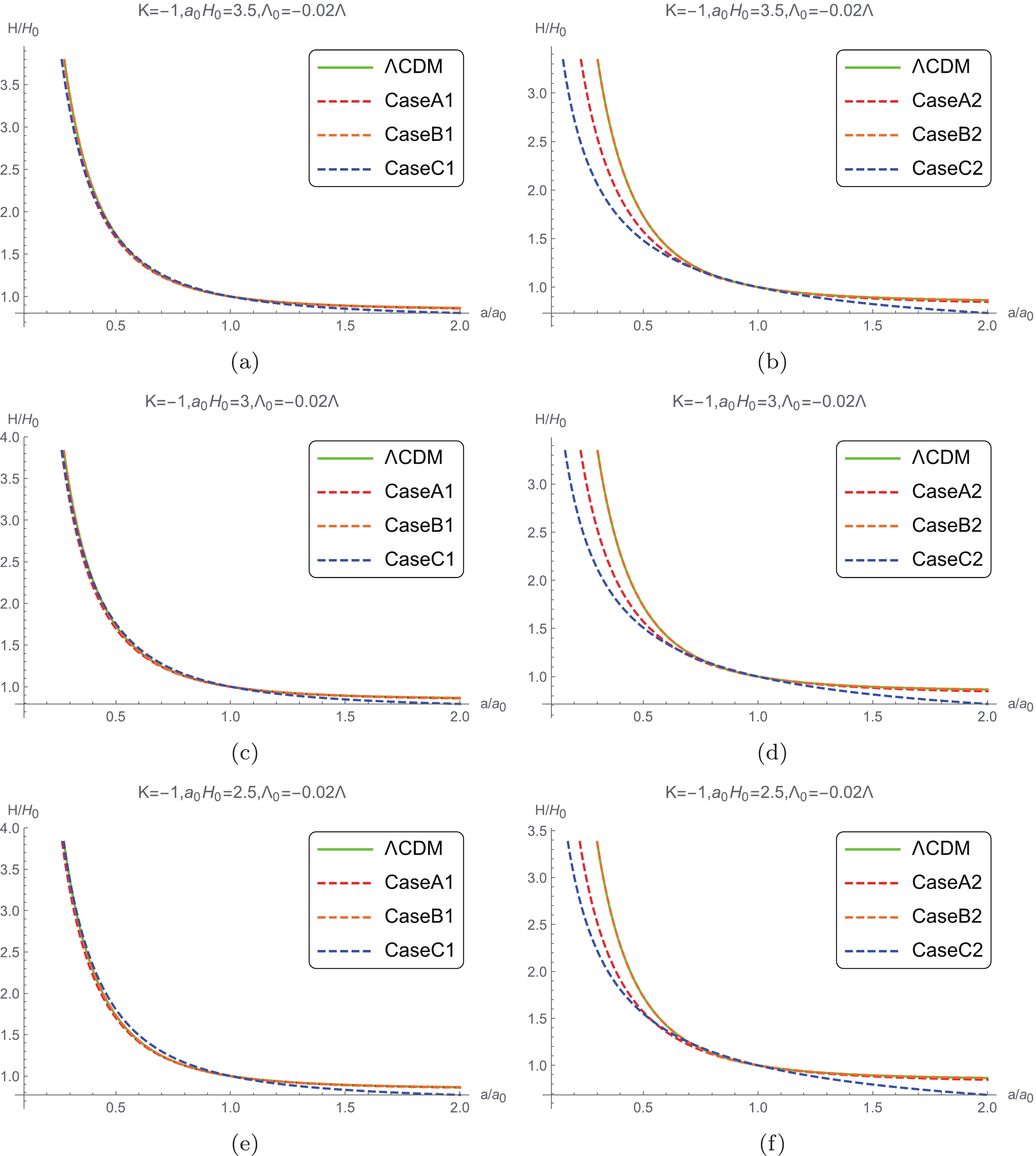
Figure 2. (color online) Hubble constant evolving with the scale factor when
$ K = -1 $ ,$ {{\Lambda }_{0}} = -0.02\Lambda $ .Figure 2 shows that the evolutions of Cases A2 and C2 in the case of
$ K = -1 $ deviate from the behavior of the ΛCDM model, while the deviations among Cases A1, B1, C1, and B2 and the ΛCDM models are very small. Figs. 1 and 2 illustrate that the evolutions in the three types of approximations, respectively, are significantly close to the evolution in the ΛCDM model when$ K = -1 $ , where$ {\mathcal K}\left(t \right) $ takes the first initial value. Because the light ray travels along the geodesic line even in the case of non-zero torsion, the redshift formula for the large scale Lorentz violation model is the same as that for the ΛCDM model,$ \begin{equation} 1{\rm+}z = \frac{{{a}_{0}}}{a}. \end{equation} $

(23) From the definition of luminosity distance, one can obtain
$ \begin{equation} {{d}_{\rm L}}\left( z \right) = \left( 1+z \right)\frac{{{d}_{\rm H}}}{\sqrt{{{\Omega }_{K}}}}\sinh \left[ \sqrt{{{\Omega }_{K}}}\int_{0}^{z}{\frac{{{H}_{0}}}{H\left( {{z}'} \right)}{\rm d}{z}'} \right], \end{equation} $

(24) where
$ {{d}_{\rm L}} $ represents the luminosity distance,$ \begin{equation} {{d}_{\rm H}} = \frac{c}{{{H}_{0}}} \end{equation} $

(25) the Hubble distance and
$ \begin{equation} {{\Omega }_{K}} = -\frac{K}{{{H}_{0}}^{2}{{a}_{0}}^{2}} \end{equation} $

(26) denotes the curvature density at present. Taking the derivative of (24) with respect to z, one can obtain
$ \begin{equation} H\left( z \right) = \frac{{{\left( 1+z \right)}^{2}}\sqrt{1-\frac{K}{{{a}_{0}}^{2}{{\left( 1+z \right)}^{2}}}{{d}_{\rm L}}^{2}\left( z \right)}}{{{d}_{\rm L}}^{\prime }\left( z \right)\left( 1+z \right)-{{d}_{\rm L}}\left( z \right)}\;. \end{equation} $

(27) With the approximation
$ \begin{equation} \sqrt{1-\frac{K{{d}_{\rm L}}^{2}\left( z \right)}{{{a}_{0}}^{2}{{\left( 1+z \right)}^{2}}}}\simeq 1-\frac{K{{d}_{\rm L}}^{2}\left( z \right)}{2{{a}_{0}}^{2}{{\left( 1+z \right)}^{2}}}, \end{equation} $

(28) and the relationship between the derivative, with respect to z and t
$ \begin{equation} \frac{\rm d}{{\rm d}t} = aH\left( a \right)\frac{\rm d}{{\rm d}a} = aH\left( a \right)\frac{{\rm d}z}{{\rm d}a}\frac{\rm d}{{\rm d}z} = -\left( 1+z \right)H\left( z \right)\frac{\rm d}{{\rm d}z}\;, \end{equation} $

(29) in the case of
$ w\approx 0 $ , equation (10) can be rewritten in terms of$ d_{\rm L} $ and z as$ \begin{aligned}[b] &\frac{{{d}_{\rm L}}^{\prime \prime}\left( z \right){{\left( 1+z \right)}^{6}}{{\left( 1-\dfrac{K{{d}_{\rm L}}^{2}\left( z \right)}{2{{a}_{0}}^{2}{{\left( 1+z \right)}^{2}}} \right)}^{2}}}{{{\left[ {{d}_{\rm L}}^{\prime }\left( z \right)\left( 1+z \right)-{{d}_{\rm L}}\left( z \right) \right]}^{3}}}-\frac\rm {1}{2}\frac{{{\left( 1+z \right)}^{4}}{{\left( 1-\dfrac{K{{d}_{\rm L}}^{2}\left( z \right)}{2{{a}_{0}}^{2}{{\left( 1+z \right)}^{2}}} \right)}^{2}}}{{{\left[ {{d}_{\rm L}}^{\prime }\left( z \right)\left( 1+z \right)-{{d}_{\rm L}}\left( z \right) \right]}^{2}}}{\rm+}\frac{K}{{{a}_{0}}^{2}}\frac{{{d}_{\rm L}}\left( z \right){{\left( 1+z \right)}^{2}}\left( 1-\dfrac{K{{d}_{\rm L}}^{2}\left( z \right)}{2{{a}_{0}}^{2}{{\left( 1+z \right)}^{2}}} \right)}{{{d}_{\rm L}}^{\prime }\left( z \right)\left( 1+z \right)-{{d}_{\rm L}}\left( z \right)} \\ &+2\frac{{{\left( 1+z \right)}^{2}}\left( 1-\dfrac{K{{d}_{\rm L}}^{2}\left( z \right)}{2{{a}_{0}}^{2}{{\left( 1+z \right)}^{2}}} \right)}{{{d}_{\rm L}}^{\prime }\left( z \right)\left( 1+z \right)-{{d}_{\rm L}}\left( z \right)}{\mathcal K}\left( z \right)-\frac{{{\left( 1+z \right)}^{3}}\left( 1-\dfrac{K{{d}_{\rm L}}^{2}\left( z \right)}{2{{a}_{0}}^{2}{{\left( 1+z \right)}^{2}}} \right)}{{{d}_{\rm L}}^{\prime }\left( z \right)\left( 1+z \right)-{{d}_{\rm L}}\left( z \right)}{\mathcal K}'\left( z \right){\rm+}\frac{1}{2}{{\mathcal K}^{2}}\left( z \right){\rm+}\frac{K}{2{{a}^{2}}}-\frac{1}{2}{{\Lambda }_{0}} = 0, \end{aligned} $

(30) together with the Case A approximation, and (12) is rewritten as
$ \begin{aligned}[b]& \frac{{{\left( 1+z \right)}^{2}}\left( 1-\dfrac{K{{d}_{\rm L}}^{2}\left( z \right)}{2{{a}_{0}}^{2}{{\left( 1+z \right)}^{2}}} \right)}{{{d}_{\rm L}}^{\prime }\left( z \right)\left( 1+z \right)-{{d}_{\rm L}}\left( z \right)}\left[ {\mathcal K}\left( z \right)-\left( 1+z \right){\mathcal K}'\left( z \right) \right] \\=& \frac{1}{3}\left( {{\Lambda }_{0}}-\Lambda \right), \end{aligned} $

(31) the Case B approximation (13) in the case of
$ w\approx 0 $ is rewritten as$ \begin{aligned}[b]& \frac{{{\left( 1+z \right)}^{2}}\left( 1-\dfrac{K{{d}_{\rm L}}^{2}\left( z \right)}{2{{a}_{0}}^{2}{{\left( 1+z \right)}^{2}}} \right)}{{{d}_{\rm L}}^{\prime }\left( z \right)\left( 1+z \right)-{{d}_{\rm L}}\left( z \right)}\left[ 2{\mathcal K}\left( z \right)-\left( 1+z \right){\mathcal K}'\left( z \right) \right]\\&{+}\frac{1}{2}{{\mathcal K}^{2}}\left( z \right){\rm+}\frac{K}{2{{a}^{2}}}{\rm+}\frac{1}{2}\left( \Lambda -{{\Lambda }_{0}} \right){\rm{ = 0}} \end{aligned} $

(32) and the Case C approximation (14) is rewritten as
$ \begin{aligned}[b]& \frac{{{2\left( 1+z \right)}^{2}}\left( 1-\dfrac{K{{d}_{\rm L}}^{2}\left( z \right)}{2{{a}_{0}}^{2}{{\left( 1+z \right)}^{2}}} \right)}{{{d}_{\rm L}}^{\prime }\left( z \right)\left( 1+z \right)-{{d}_{\rm L}}\left( z \right)}[\left(2+3w_0\right){\mathcal K}\left( z \right) \\&-\left( 1+z \right){\mathcal K}'\left( z \right) ]+\left(1+3w_0\right){{\mathcal K}^{2}}\left( z \right) = \left(1+w_0\right)\Lambda_{0} \end{aligned} $

(33) The distance modulus defined by
$ \begin{equation} \mu = 25+5{\rm{log}}\left(\frac{d_{\rm L}}{M{\rm{pc}}}\right) \end{equation} $

(34) is a way of expressing the distance often used in astronomical observation [16]. Figs. 3 and 4 present the evolution of the luminosity distance versus redshift predicted by the present model.

Figure 3. (color online) Luminosity distance evolving with the redshift when
$ K = +1, {{w}_{0}} = -1, {{\Lambda }_{0}} = -0.02\Lambda $ .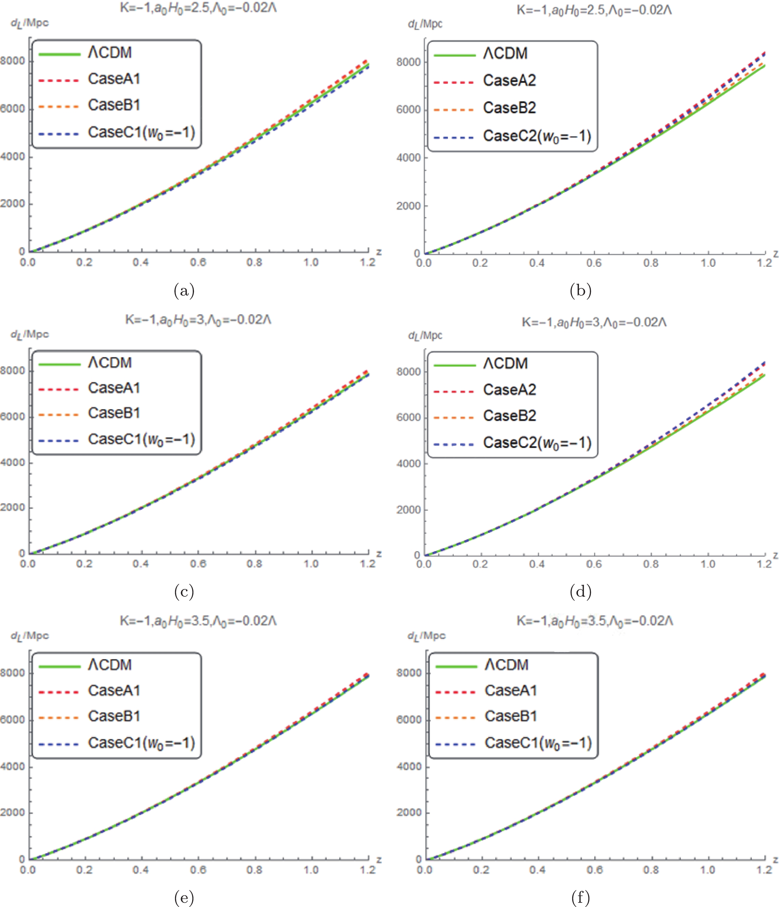
Figure 4. (color online) Luminosity distance evolving with the redshift when
$ K = -1, {{w}_{0}} = -1, \;{{\Lambda }_{0}} = -0.02\Lambda $ . -
The modified Friedmann Eq. (17) of the large scale Lorentz violation model can be expressed as
$ \begin{equation} \frac{\rho }{3{{H}^{2}}}{\rm+}\frac{{{\Lambda }_{0}}}{3{{H}^{2}}}-\frac{2\mathcal K}{H}-{{\left( \frac{\mathcal K}{H} \right)}^{2}}-\frac{K}{{{a}^{2}}{{H}^{2}}} = 1 \end{equation} $

(35) and
$ \begin{equation} {{\Omega }_{M}}+{{\Omega }_{\rm eff}} = 1, \end{equation} $

(36) where
$ \begin{equation} {{\Omega }_{M}} = \frac{\rho }{3{{H}^{2}}} \end{equation} $

(37) denotes the matter density, while
$ {{\Omega }_{\rm eff}} = \dfrac{{{\Lambda }_{0}}}{3{{H}^{2}}}-\dfrac{2\mathcal K}{H}- $ $ {{\left(\dfrac{\mathcal K}{H} \right)}^{2}}-\dfrac{K}{{{a}^{2}}{{H}^{2}}} $ represents the contributions of the bare cosmological constant, contortion, and spatial curvature. The minimum value for$ \Lambda_0 $ in the case of$ K = +1, -1 $ is presented in Fig. 5. Utilizing the modified Friedmann equation, for every type of approximation model, one can obtain the evolution of the matter energy density with time. The evolution of$ {{\Omega }_{M}} $ in the three approximation model types at different values of$ {{\Lambda }_{0}} $ is presented in Fig. 6.$ {{\Omega }_{M}} $ will decrease to be negative along with the increase in$ {{\Lambda }_{0}} $ beyond a critical value,$ \Lambda _{\rm max} $ . This triggers a constrain condition on the$ \Lambda_{0} $ value,
Figure 5. (color online) Evolution of the
$ {{\Lambda }_{\min }} $ versus$ {{a}_{0}}{{H}_{0}} $ .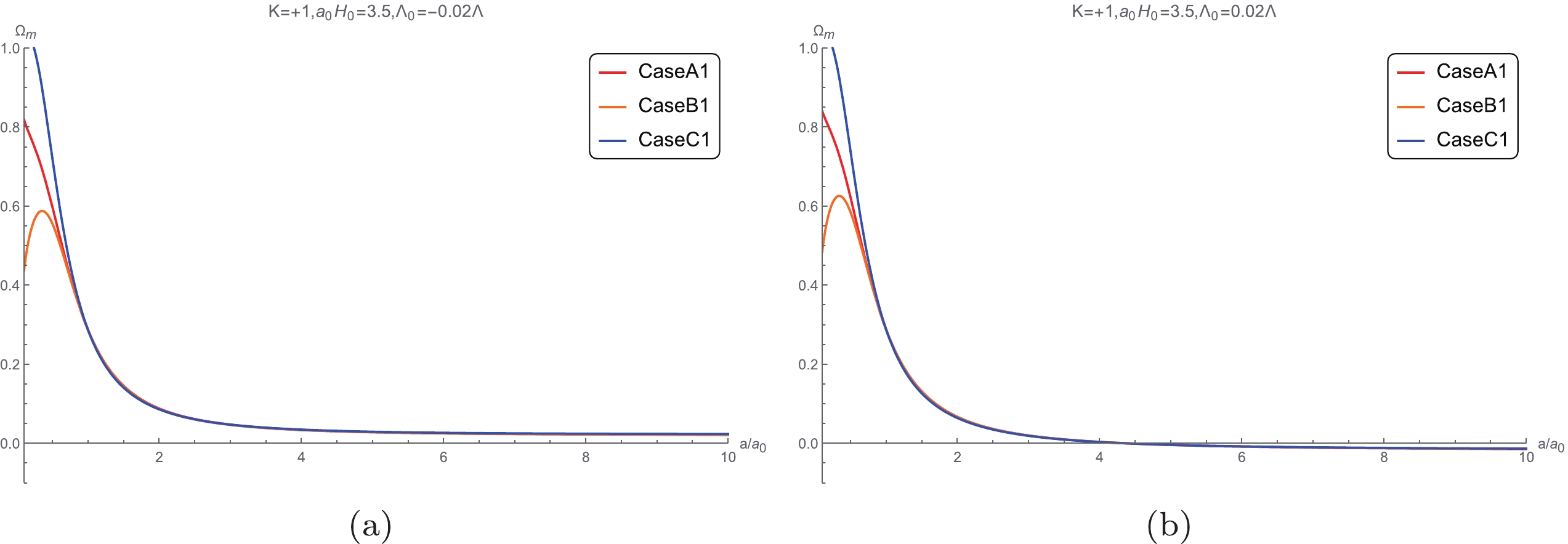
Figure 6. (color online) Evolution of the matter density
$ \Omega_{M} $ versus the scale factor.$ \begin{equation} 1-\frac{{{\Lambda }_{0}}}{3{{H}^{2}}}+\frac{2\mathcal K}{H}+{{\left( \frac{\mathcal K}{H} \right)}^{2}}+\frac{K}{{{a}^{2}}{{H}^{2}}}\ge 0, \end{equation} $

(38) to ensure that
$ {{\Omega }_{M}}\ge 0 $ . Constrain (38) sets a maximum$ \Lambda_{\max} $ ,$ \begin{equation} {{\Lambda }_{\max }} = 3{{H}^{2}}+6H\mathcal{K}+3{{\mathcal{K}}^{2}}+\frac{3K}{{{a}^{2}}}, \end{equation} $

(39) for the
$ \Lambda_{0} $ value. When$ {{\Lambda }_{0}} > {\Lambda }_{\max } $ , the value of$ {{\Omega }_{M}} $ will be less than zero. Tables 1 and 2 present the$ {\Lambda }_{\max } $ values for all the cases in consideration.$ K=+1 $ 

$\Lambda_{\rm max}$ 

$ a_0 H_0 = 2 $ 

$ (\Omega_k=-0.25) $ 

$ a_0 H_0 = 2.5 $ 

$ (\Omega_k=-0.16) $ 

$ a_0 H_0 = 3 $ 

$ (\Omega_k=-0.11) $ 

$ a_0 H_0 = 3.5 $ 

$ (\Omega_k=-0.08) $ 

Case A1 0.0008 0.0007 0.0007 0.0006 Case A2 0.0012 0.0014 0.0015 0.0015 Case B1 0.0008 0.0007 0.0007 0.0006 Case B2 0.0012 0.0014 0.0015 0.0016 Case C1
($ w_0=-1 $ )

0.0008 0.0007 0.0007 0.0006 Case C2
($ w_0=-1 $ )

0.0012 0.0015 0.0015 0.0016 Case C1
($ w_0=-8/9 $ )

0.0008 0.0007 0.0007 0.0006 Case C2
($ w_0=-8/9 $ )

0.0013 0.0016 0.0017 0.0018 Case C1
($ w_0=-7/9 $ )

0.0008 0.0007 0.0007 0.0006 Case C2
($ w_0=-7/9 $ )

0.0013 0.0016 0.0018 0.0019 Case C1
($ w_0=-2/3 $ )

0.0008 0.0007 0.0006 0.0006 Case C2
($ w_0=-2/3 $ )

0.0014 0.0018 0.002 0.0022 Case C1
($ w_0=-1/3 $ )

0.0008 0.0006 0.0006 0.0006 Case C2
($ w_0=-1/3 $ )

0.0025 0.0046 0.0056 0.0062 Table 1. Values of
$ \Lambda_{\rm max} $ when$ K = +1 $ $ K=-1 $ 

$\Lambda_{\rm max}$ 

$ a_0 H_0 = 1.5 $ 

$ (\Omega_k=0.44) $ 

$ a_0 H_0 = 2 $ 

$ (\Omega_k=0.25) $ 

$ a_0 H_0 = 2.5 $ 

$ (\Omega_k=0.16) $ 

$ a_0 H_0 = 3 $ 

$ (\Omega_k=0.11) $ 

$ a_0 H_0 = 3.5 $ 

$ (\Omega_k=0.08) $ 

Case A1 0.0004 0.0005 0.0005 0.0005 0.0005 Case A2 0.0023 0.002 0.0019 0.0018 0.0018 Case B1 0.0004 0.0004 0.0005 0.0005 0.0005 Case B2 0.0023 0.002 0.0019 0.0019 0.0018 Case C1
($ w_0=-1 $ )

0.0003 0.0004 0.0005 0.0005 0.0005 Case C2
($ w_0=-1 $ )

0.015 0.0027 0.0023 0.0021 0.002 Case C1
($ w_0=-8/9 $ )

0.0003 0.0004 0.0005 0.0005 0.0005 Case C2
($ w_0=-8/9 $ )

0.0033 0.0033 0.0026 0.0024 0.0023 Case C1
($ w_0=-7/9 $ )

0.0003 0.0004 0.0005 0.0005 0.0005 Case C2
($ w_0=-7/9 $ )

0.0032 0.0032 0.0032 0.0028 0.0026 Case C1
($ w_0=-2/3 $ )

0.0003 0.0004 0.0004 0.0004 0.0005 Case C2
($ w_0=-2/3 $ )

0.0185 0.0091 0.0054 0.0037 0.0031 Case C1
($ w_0=-1/3 $ )

0.001 0.0005 0.0005 0.0005 0.0005 Case C2
($ w_0=-1/3 $ )

0.0147 0.0119 0.0105 0.0097 0.0092 Table 2. Values of
$\Lambda_{\max}$ when$ K = -1. $ It can be observed that
$ {{\Omega }_{M}} $ will decrease to be negative whenever$ {{\Lambda }_{0}} $ is positive. Hence, the reasonable values of$ {{\Lambda }_{0}} $ should be non-positive, i.e.,$ {{\Lambda }_{\rm max}}\approx 0 $ . In [14, 15], the authors point out that there is a critical value for$ {{\Lambda }_{0}} $ , named$ {{\Lambda }_{0-{\rm crit}}} $ , which represents the separation of two phases in the evolution pattern of$ {{\Lambda }_{\rm eff}} $ versus t, i.e.,$ {{\Lambda }_{\rm eff}} $ decreases monotonically along with the increase in t when$ {{\Lambda }_{0}}\le {{\Lambda }_{0-{\rm crit}}} $ , while its evolution has a local minimum when$ {{\Lambda }_{0}}>{{\Lambda }_{0-{\rm crit}}} $ , and the$ {{\Lambda }_{0-{\rm crit}}} $ is approximately zero. In other words,$ {{\Lambda }_{\rm eff}} $ monotonically decreases when$ {{\Lambda }_{0}} $ emerges from the string landscape, while$ {{\Lambda }_{\rm eff}} $ has a local minimum when$ {{\Lambda }_{0}} $ originates from the swampland. Tables 3 and 4 present the values of$ {{\Lambda }_{0-{\rm crit}}} $ for all the cases of approximation in consideration. In [17], it is demonstrated that$ V\left(\phi \right) $ is a monotonically decreasing quintessence potential if$ {{\Lambda }_{0}} $ is negative or from the string landscape, while$ V\left(\phi \right) $ is a meta-stable de Sitter one if$ {{\Lambda }_{0}} $ is positive or from the swampland when$ {{\Lambda }_{\rm eff}} $ is simulated by a scalar quintessence field potential$ V\left(\phi\right) $ . The dependence of$ {{\Lambda }_{0{\rm{-}}{\rm crit}}} $ on different values of$ a_0H_0 $ in both the cases of$ K = +1 $ and$ K = -1 $ is investigated in this study, and the numerical results are presented in Tables 3 and 4. A specific example solution of the$ {{\Lambda }_{{\rm{eff}}}} $ evolution pattern transition with the dependence on$ \Lambda_{0} $ is presented in Fig. 7. Figure 5 demonstrates that$ {{\Lambda }_{\min }} $ is positive if$ {{a}_{0}}{{H}_{0}} $ takes a value less than 2 in the case of$ K = +1 $ , i.e.,$ {{\Lambda }_{\min }}>{{\Lambda }_{\max }} $ , such that$ \Lambda_{0{\rm{-}}{\rm crit}} $ does not make any sense in the case of$ K = +1 $ and$ {{a}_{0}}{{H}_{0}}\ge 2 $ .$ K=+1 $ 

$ K=0 $ 

$ \Lambda_{0-{\rm crit}} $ 

$ a_0 H_0 = 2.5 $ 

$ a_0 H_0 = 3 $ 

$ a_0 H_0 = 3.5 $ 

Case A1 −0.072 −0.064 −0.059 0.05 Case A2 −0.14 −0.0159 −0.167 −0.18 Case B1 −0.094 −0.083 −0.078 −0.066 Case B2 −0.154 −0.176 −0.187 −0.2144 Case C1
($ w_0=-1 $ )

0 0 0 0 Case C2
($ w_0=-1 $ )

0 0 0 0 Case C1
($ w_0=-8/9 $ )

0.162 0.152 0.146 0.119 Case C2
($ w_0=-8/9 $ )

0.09 0.086 0.083 0.075 Case C1
($ w_0=-7/9 $ )

none none none none Case C2
($ w_0=-7/9 $ )

0.173 0.164 0.164 0.152 Case C1
($ w_0=-2/3 $ )

none none none none Case C2
($ w_0=-2/3 $ )

0.246 0.235 0.228 0.225 Case C1
($ w_0=-1/3 $ )

none none none none Case C2
($ w_0=-1/3 $ )

0.354 0.368 0.375 0.397 Table 3. Values of
$\Lambda_{\rm 0-crit}$ in the case of$ K = +1 $ $ K=-1 $ 

$ K=0 $ 

$\Lambda_{0-{\rm crit}}$ 

$ a_0 H_0 = -1.5 $ 

$ a_0 H_0 = -2 $ 

$ a_0 H_0 = -2.5 $ 

$ a_0 H_0 = -3 $ 

$ a_0 H_0 = -3.5 $ 

Case A1 −0.023 −0.033 −0.038 −0.041 −0.044 −0.05 Case A2 −0.214 −0.208 −0.203 −0.198 −0.195 −0.187 Case B1 −0.03 −0.042 −0.049 −0.053 −0.056 −0.066 Case B2 −0.284 −0.262 −0.248 −0.239 −0.233 −0.2144 Case C1
($ w_0=-1 $ )

0 0 0 0 0 0 Case C2
($ w_0=-1 $ )

0 0 0 0 0 0 Case C1
($ w_0=-8/9 $ )

0.05 0.086 0.102 0.107 0.115 0.119 Case C2
($ w_0=-8/9 $ )

none 0.03 0.052 0.059 0.064 0.075 Case C1
($ w_0=-7/9 $ )

none none none none none none Case C2
($ w_0=-7/9 $ )

none 0.079 0.104 0.118 0.131 0.152 Case C1
($ w_0=-2/3 $ )

none none none none none none Case C2
($ w_0=-2/3 $ )

0.03 0.15 0.173 0.189 0.198 0.225 Case C1
($ w_0=-1/3 $ )

none none none none none none Case C2
($ w_0=-1/3 $ )

0.203 0.25 0.278 0.309 0.343 0.397 Table 4. Values of
$\Lambda_{\rm 0-crit}$ in the case of$ K = -1 $ 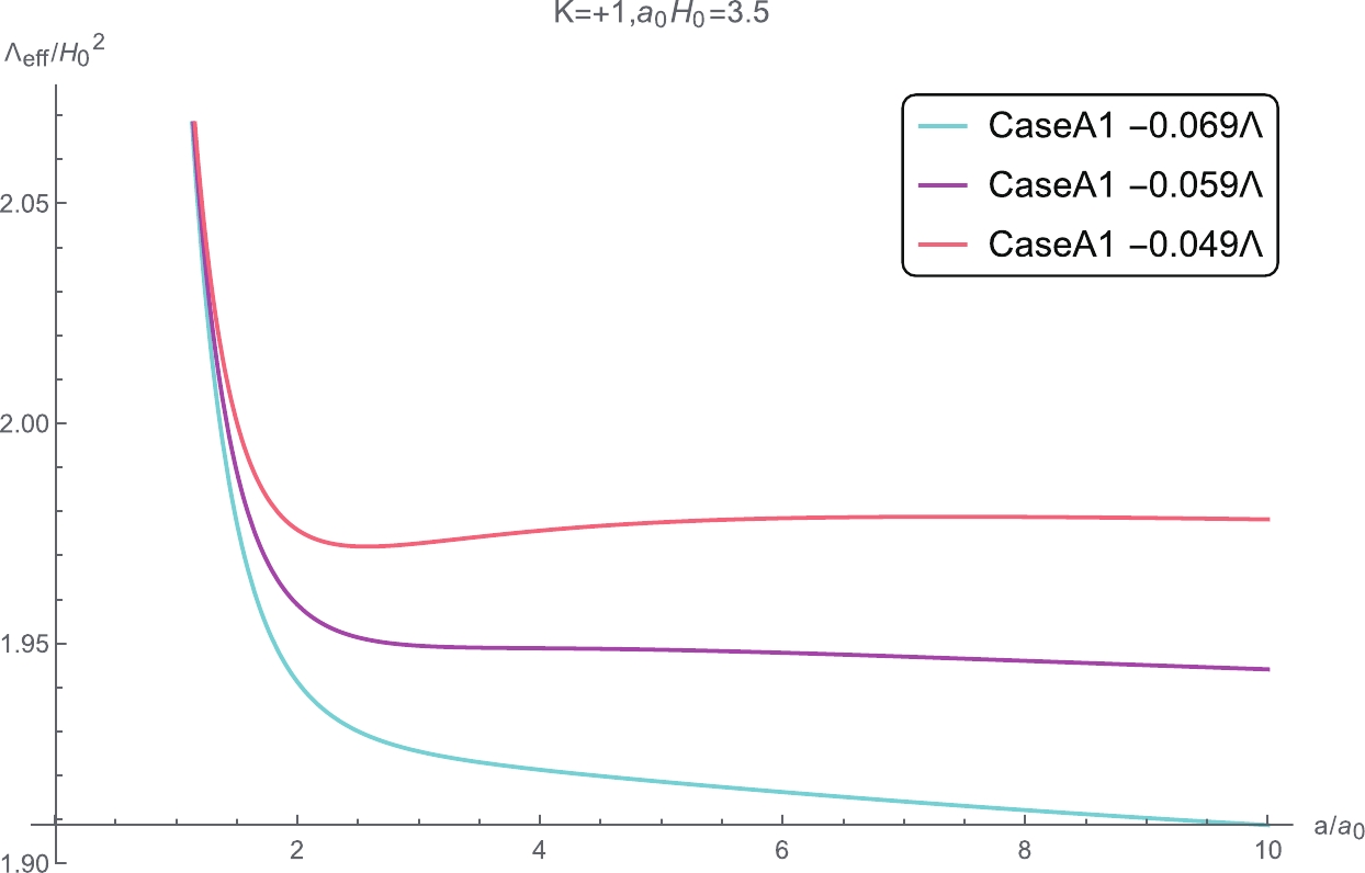
Figure 7. (color online) Evolution pattern of
$ {{\Lambda }_{{\rm{eff}}}} $ versus scale factor shifting from a monotonically decreasing quintessence type to a local minimal type with a dependence on$ \Lambda_0 $ .When the
$ w_0 $ value of Case C2 is greater than$ -\dfrac{8}{9} $ ,$ \Lambda_{\rm eff} $ exhibits a quintessence like potential that decreases monotonically over time without a local minimum, i.e., there is no solution for$ {{\Lambda }_{0-{\rm crit}}} $ . It is possible that the behavior is caused by the fixed value of$ w_0 $ , other than an evolved one in the equation of state for dark partner. A similar conclusion is reached based on the large-scale Lorentz violation model without spatial curvature in [14, 15]. When$ {{w}_{0}}>-\dfrac{8}{9} $ , the model prediction on the luminosity distance modulus versus redshift curve of Case C2 does not match observation one in the case of$ K = 0 $ ; however, the prediction on the evolution luminosity distance modulus is compatible with observation one in the case of$ K\ne 0 $ . The spatial non-flat Case C2 with$ {{w}_{0}}>-\dfrac{8}{9} $ cannot be excluded by observation, similar to the spatial flat case presented in [14, 15]. However, we find that the$ {{\Lambda }_{0-{\rm crit}}} $ of Case C is always greater than$ {{\Lambda }_{\max }} $ when$ {{w}_{0}}>-1 $ from Tables 1, 2, 3 and 4, i.e., the solution of$ {{\Lambda }_{0-{\rm crit}}} $ for Case C does not exist within the range of values that can be taken for$ \Lambda_{0} $ when$ {{w}_{0}}>-1 $ . Comparisons of the luminosity distance$ {{d}_{\rm L}} $ curve versus redshift z among three models of approximation and the ΛCDM model are presented in Fig. 8 to Fig. 13.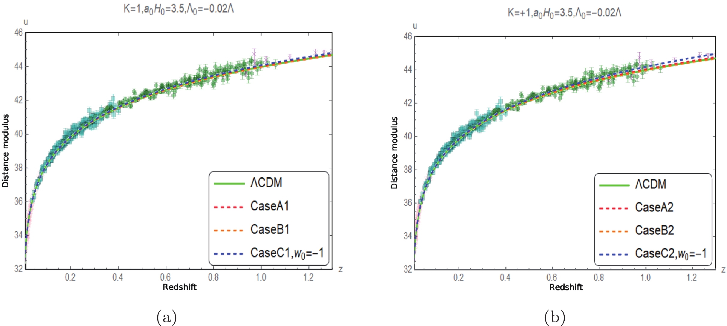
Figure 8. (color online) Comparison of the measured distance modulus [16] with the corresponding predicted values when
$ K = +1 $ ,$ {{\Lambda }_{0}} = -0.02\Lambda $ , and$ {{a}_{0}}{{H}_{0}} = 3.5 $ .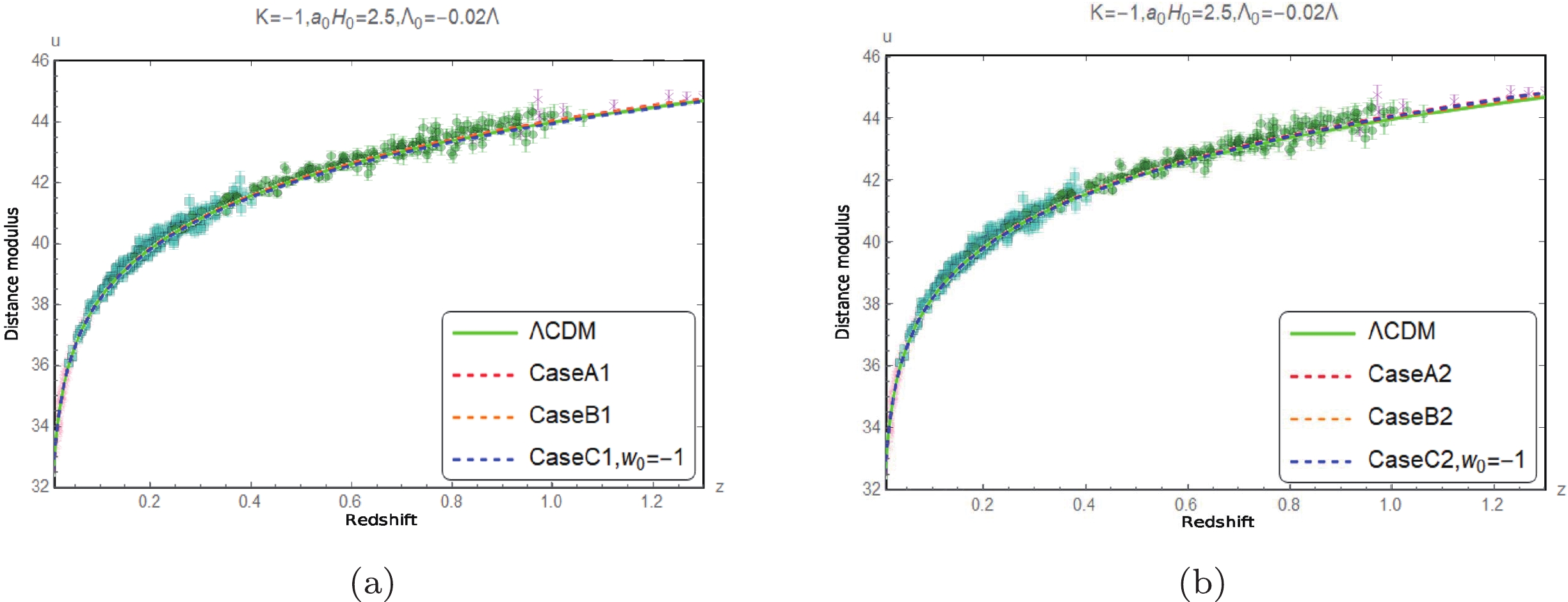
Figure 13. (color online) Comparison of the measured distance modulus [16] with the corresponding predicted values when
$ K = -1 $ ,$ {{\Lambda }_{0}} = -0.02\Lambda $ , and$ {{a}_{0}}{{H}_{0}} = 2.5 $ .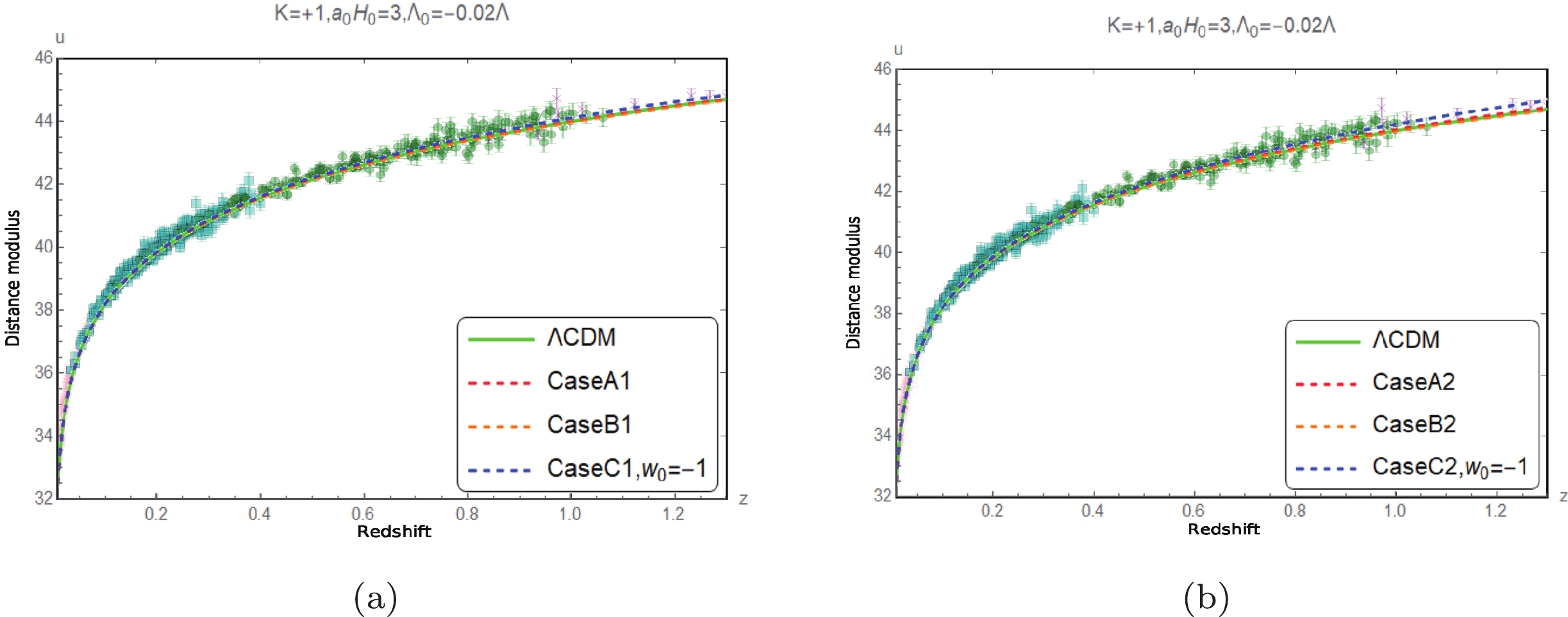
Figure 9. (color online) Comparison of the measured distance modulus [16] with the corresponding predicted values when
$ K=+1 $ ,$ {{\Lambda }_{0}}=-0.02\Lambda $ , and$ {{a}_{0}}{{H}_{0}}=3 $ .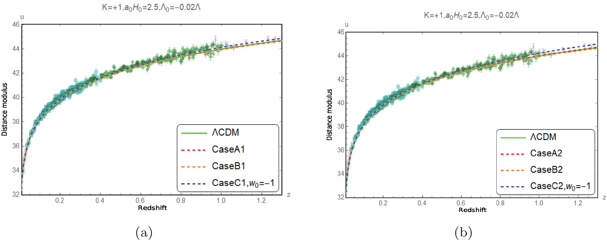
Figure 10. (color online) Comparison of the measured distance modulus [16] with the corresponding predicted values when
$ K=+1 $ ,$ {{\Lambda }_{0}}=-0.02\Lambda $ , and$ {{a}_{0}}{{H}_{0}}=2.5 $ .
Figure 11. (color online) Comparison of the measured distance modulus [16] with the corresponding predicted values when
$ K=-1 $ ,$ {{\Lambda }_{0}}=-0.02\Lambda $ , and$ {{a}_{0}}{{H}_{0}}=3.5 $ .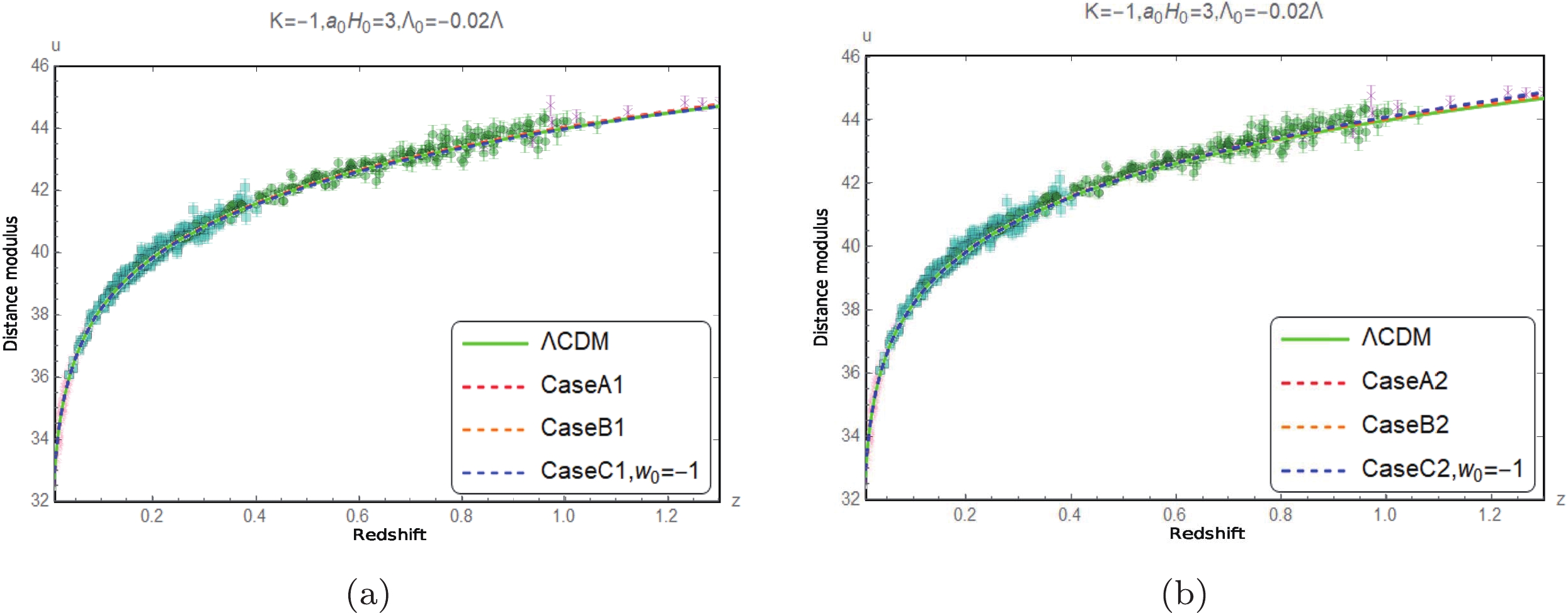
Figure 12. (color online) Comparison of the measured distance modulus [16] with the corresponding predicted values when
$ K=-1 $ ,$ {{\Lambda }_{0}}=-0.02\Lambda $ , and$ {{a}_{0}}{{H}_{0}}=3 $ .Figs. 8 to 13 show that the predictions of the luminosity distance modulus of the three cases of the approximation models for different spatial curvature values with the restricted range of
$ \Lambda_0 $ values are all compatible with the observational data within the error range [16]. In other words, the luminosity distance observations are inefficient in choosing the models.The evolutions of
$ {{\Omega }_{\Lambda }} = \dfrac{{{\Lambda }}}{3{{H}^{2}}} $ in ΛCDM model,$ {{\Omega }_{\rm eff}}\left(K = 0 \right) $ in the large-scale Lorentz violation model without spatial curvature, and$ {{\Omega }_{\rm eff}}\left(K = \pm 1 \right) $ in the large-scale Lorentz violation model with spatial curvature are presented in Fig. 14, which demonstrates that the evolution behaviors of$ {{\Omega }_{\Lambda }} $ ,$ {{\Omega }_{\rm eff}}\left(K = 0 \right) $ , and$ {{\Omega }_{\rm eff}}\left(K = \pm 1 \right) $ are similar; hence, their contributions are degenerate in the results.
Figure 14. (color online) Evolution of
$ {{\Omega }_{\Lambda }} $ ,$ {{\Omega }_{\rm eff}}\left(K = 0 \right) $ ,$ {{\Omega }_{\rm eff}}\left(K = \pm 1 \right) $ , and$ \Omega_k $ .Fig. 15 illustrates the evolution of the energy density of the spatial curvature
$ \Omega_K = -\dfrac{K}{{{a}^{2}}{{H}^{2}}} $ versus scale factor a based on the modified Friedmann equations for both the cases of$ K = +1 $ and$ K = -1 $ , respectively. The maximum and minimum values of$ {{\Omega }_{K}} $ can also be obtained from the evolution of$ \Omega_K $ . When$ K = +1 $ , Case C1 exhibits the minimum curvature energy density of$ {{\Omega }_{K}} = -0.34 $ , while Case A1 has the maximum of$ {{\Omega }_{K}} = 0.6 $ when$ K = -1 $ . The evolution of the absolute values of the curvature energy densities always increase at the first stage, then decrease to zero after reaching the maximum. Figs. 1 to 2 can also indicate the evolution tendency of the absolute values of the curvature densities, where the evolution of H decreases, and$ {{a}^{2}}{{H}^{2}} $ has a minimum value during evolution.
Figure 15. (color online) Evolution of
$ {{\Omega }_{K}} $ with the scale factor.The evolution of the acceleration of the universe expansion
$ \ddot a $ can also be obtained by the modified Friedmann equations and the approximations considered. The evolution of$ \ddot{a} $ versus scale factor a is presented in Fig. 16, from which it can be approximately obtained that the expansion of the universe decelerates before the cosmic scale factor reaches$ 0.5a_0 $ , and the universe starts accelerating afterwards. This conclusion is consistent with the observed universe experiencing the transition from decelerating expansion to accelerating expansion, thus providing further side proof for the confidence level of the large scale Lorentz violation model with non-vanishing spatial curvature.
Figure 16. (color online) Evolution of
$ \ddot{a} $ versus the scale factor. -
The cause of the
$ H_0 $ tension between high and low redshift measurements remains unknown to date, although several solutions to$ H_0 $ tension have been proposed. It was suggested that this was owing to systematic errors; however, these claims were quickly disproved [18–21]. The gravitational waves from the binary neutron star (BNS) merger may be able to provide independent measurements of$ H_0 $ [22], although future observations should be able to reduce the error [23–30]. However, this current measurement method has a large error (due to being a single event); hence, it does not resolve the tension between$ H_0 $ measurements. Furthermore, as one of the simplest alternatives to the ΛCDM model, quintessence fields with smooth potential energy, rolling slowly or at moderate velocity in the non-flat FRW universe, are expected to resolve the tension between Hubble constant measurements. However, after combining the latest CMB, SNe, and BAO data, it was deduced that this model does not reduce the Hubble constant tension [31].A previous study [32] presents a novel solution to the Hubble constant problem. The solution is based on the Simsilun simulation (relativistic simulation of the large scale structure of the Universe) with the ray-tracing algorithm implemented; the Simsilun simulation relativistic and nonlinear evolutions of cosmic structures lead to the emerging spatial curvature phenomenon, where the mean spatial curvature evolves from spatial flatness of the early universe towards the slightly curved present-day universe. The deduced Hubble constant,
$ H_0 = (68.1\pm $ $ 2.0){\rm{km}}/({\rm{s}}\cdot {\rm{Mpc}}) $ , alleviates the tension between the CMB and distance ladder measurements of the Hubble constant, and it is argued that the$ H_0 $ tension is a manifestation of rigidity in the FLRW geometry.At the current stage, the existence of spatial curvature appears to be a viable solution to the Hubble constant problem. In fact, we can also counter that the tension is an indirect evidence of the emerging spatial curvature. From the perspective of astronomical observations, no direct measurement of spatial curvature has yet been obtained at low redshifts (the constraint obtained is also only the result of fitting FLRW to the data, which is not equivalent to a direct measurement).
In conclusion, although the large scale Lorentz violation model with non-vanishing spatial curvature has one more cosmological scale contortion parameter than the ΛCDM model with non-vanishing spatial curvature, the inputs are well constrained in a variety of ways, and the theoretical predictions of distance modulus, cosmic expansion acceleration, etc., agree well with observations.
The temperature fluctuation in the CMB power spectra can fix the cosmological parameters of the ΛCDM model strictly. The Hubble constant predicted by the large scale Lorentz violation with a non-vanishing spatial curvature is also constrained by the CMB data and compared with the one predicted by the CMB data based on ΛCDM model, to evaluate the improvement on the
$ H_0 $ tension problem by the large scale Lorentz violation with a non-vanishing spatial curvature model. The cosmological parameters of the specific cosmological model, such as the ΛCDM model, can be obtained from CMB data, using numerical software, such as the Code for Anisotropies in the Microwave Background (CAMB). It is pointed out that the spatial flatness assumption may be responsible for the$ H_0 $ tension, and the non-vanishing spatial curvature is an alternative choice. This study provides a feasible solution to$ H_0 $ tension by investigating the constrain on the spatial curvature provided by the large scale Lorentz violation cosmological model with spatial curvature. We infer that the non-vanishing of the spatial curvature is compatible with the present observation. The model provides a feasible premise to solve the$ H_0 $ tension problem using the spatial non-flat cosmological model. The numerical software (such as CAMB) needs to be extended to the model with non-trivial contortion distribution to present the$ H_0 $ value in this type of models.
Spatial curvature and large scale Lorentz violation
- Received Date: 2021-12-05
- Available Online: 2022-06-15
Abstract: The tension between the Hubble constant values obtained from local measurements and cosmic microwave background (CMB) measurements has motivated us to consider the cosmological model beyond ΛCDM. We investigate the cosmology in the large scale Lorentz violation model with a non-vanishing spatial curvature. The degeneracy among spatial curvature, cosmological constant, and cosmological contortion distribution makes the model viable in describing the known observational data. We obtain some constraints on the spatial curvature by comparing the relationship between measured distance modulus and red-shift with the predicted one, the evolution of matter density over time, and the evolution of effective cosmological constant. The implications of the large scale Lorentz violation model with the non-vanishing spatial curvature under these constrains are discussed.


 DownLoad: