Mass spectra and decay of mesons under strong external magnetic field

Over the years, studies on the nature and state of strong interacting substances under extreme conditions have attracted much attention, where extreme conditions include high temperature and finite baryon chemical potential [1-3], as well as strong magnetic fields. In this paper we discuss the effects of finite magnetic fields on strong interacting matter [4-14]. Magnetic field changes are closely related to high-energy nuclear collisions, dense stars and cosmic phase transitions. The maximum magnetic field observed in nature is about $ 10^{12}- $$ 10^{13} ~~ \mathrm{Gauss} $ in pulsars, the maximum magnetic field on the surface of some magnetospheric stars is around $ 10^{14}-10^{15} ~~ \mathrm{Gauss} $, and its internal field is estimated to be $ 10^{18}-10^{20} ~~ \mathrm{Gauss} $. In the early stage of the RHIC non-central heavy ion collision, there is also an evidence of a very strong and instantaneous magnetic field. Depending on the energy of the collision and impact parameters, the magnetic field produced in RHIC is about $ eB\sim1.5m_{\pi}^{2}\sim $$ 0.03 ~~ \mathrm{GeV^{2}} $, and $ eB\sim15 m_{\pi}^{2}\sim0.3 ~~ \mathrm{GeV^{2}} $ in the LHC [15-18]. On the other hand, the quark–gluon plasma produced in high energy heavy-ion collisions went through many stages in the process of evolution. A large number of hadrons including π are produced, freeze out and then survive in the final state [19]. Therefore, the existence of the background magnetic field generated in the heavy ion experiment may affect the properties of the early "charged quarks" in the collision. Although this strong magnetic field lasts a very short time and disappears very fast, it may affect the properties of the hadrons formed by these "magnetized" quarks. Even the properties of neutral mesons may be affected by external magnetic fields produced in the early stage of heavy ion collisions [16, 17].

This paper is based on the two-flavor NJL model [20-23]. We calculate the energy gap equation by the mean field approximation. We use the Ritus method to calculate the decay triangle diagram and self-energy in the magnetic field through Random Phase Approximation (RPA), then we obtain the meson decay width and meson–quark coupling constant. Our result shows that as quarks which constitutes mesons are magnetized under a magnetic field, the mass of σ grows, whereas the mass of $ \pi_0 $ changes very little at low temperature, and the coupling constants $ g_{\sigma qq} $ and $ g_{\pi_{0}qq} $ are significantly larger than that without a magnetic field.

The organization of the paper is as follows. In Sec. II, we give the effective thermodynamic potential. In Sec. III, we calculate the mass spectra of mesons and the decay constant of $ \sigma\rightarrow \pi_{0}\pi_{0} $. Section IV gives the numerical results of our work. Finally we summarize and discuss some possible extension of our work in Sec. V.

The Lagrangian density of the SU(2) NJL model is

The Lagrangian density has $ SU_V(2)\times{SU_A(2)}\times{U_V(1)} $ symmetry, where $ SU_V(2) $ corresponds to the chiral symmetry, $ SU_A(2) $ corresponds to the conservation of isotopic spin, and $ U_V(1) $ corresponds to the conservation of baryon numbers. In the formula, ψ and $ \bar\psi $ are quark fields. When the isospin symmetry is satisfied, we have $ m_{\mu} = m_{d} = m_{0} $. $ D^{\mu} = \partial^{\mu}+{\rm i}eA^{\mu} $ is covariant differentiation, $ A^{\mu} = \delta_{0}^{\mu}A^{0} $ and $ A^{0} = -{\rm i}A^{4} $ are gauge fields. G is the four-quark coupling constant. The Pauli matrix $ \tau_{i}(i = 1,2,3) $ is defined in the isospin space.

The thermodynamic potential can be expressed as

with the partition function

where V is the volume, $ \beta = \dfrac{1}{T} $. $ \mu = {\rm dig}(\mu_{u},\mu_{d}) $ is the chemical potential of the quark. Following the calculations such as [24, 25], we have the thermodynamic potential under the mean field approximation,

where $ \Omega_{q} $ is the contribution of the quark part

In this formula $ S^{-1}(p) = \gamma^{\mu}p_{\mu}-m_{q},\; p^{0} = {\rm i}\omega_{n} = (2n+1)\pi T $. It is known that

Using of the summation formula [26]

one can obtain

where, $ E_{p} = \sqrt{p_{3}^{2}+m_{q}^{2}} $. Regardless of the chemical potential, $ \mu = 0 $, the formula will change to

If the magnetic field is added, one will find that

then, the thermodynamic potential becomes

where, $ E_f = \sqrt{p_{3}^{2}+2 n\left|Q_{f} B\right|+m_{q}^{2}} $, $ \alpha_{n} = 2-\delta_{n0} $, charge $ Q = $$ {\rm diag}(Q_{u},Q_{d}) $ to the external magnetic field $ \boldsymbol{B} = (0,0,B) $ in z-direction, f is flavor u or d.

The energy gap equation can be derived from the derivative of the thermodynamic potential. From the energy gap equation we can calculate the mass of the quark and the single-loop self-energy through RPA [21-23, 27] in a two-flavor NJL model. As for the selection of magnetical quark propagators, usually we have two methods: Ritus scheme [18, 28-36] and the Schwinger scheme [11, 12]. In this paper, the Ritus scheme is used to deal with propagators, which is described in coordinate space,

where,

and the magnetic field related terms are

the term $ g_n^{sf}(x_1,p_2) = \phi_n(x_1-s_fp_2/|Q_fB|) $ is determined by hermite polynomial $ H_{n}(\zeta) $.

Here, $ \tilde{p} = (p_{0},0,p_{2},p_{3}) $ is the momentum of the Fourier transform, and $ \bar{p} = (p_{0},0,-s_{f}\sqrt{2n|Q_{f}B|},p_{3}) $ is the conserved Ritus momentum. $ s_{f} = sgn(Q_{f}B) $, $ Q_{f} = (2/3,-1/3) $, and f means quark flavor. $ I_{n} = 1-\delta_{n0} $, where n is the landau energy level.

To illustrate the Ritus scenario clearly, we use neutral mesons as a simple example. In this case, the meson momentum $ k = (\omega,k_{1},k_{2},k_{3}) $ is conserved for neutral mesons which do not interact with the magnetic field. The corresponding meson polarization functions in the momentum space are the Fourier transforms of their expressions in the coordinate space,

Using random phase approximation, one can obtain

The mass of a meson is defined by the pole of the denominator at zero momentum

The polarization function is [37],

where,

and

with $ \epsilon_{\pi_0} = 0 $ and $ \epsilon_{\sigma} = 2m_q $.

Under zero magnetic field

where $ E_f = \sqrt{{\boldsymbol{p}}^{2}+m_{q}^{2}} $ for the distribution function $ f_{F}(E_{f}) = \dfrac{1}{{\rm e}^{\beta E_{f}+1}} $. After considering the magnetic field, one can make the substitution in Eq. (11). Therefore, the self-energy of mesons under external magnetic field can be further obtained,

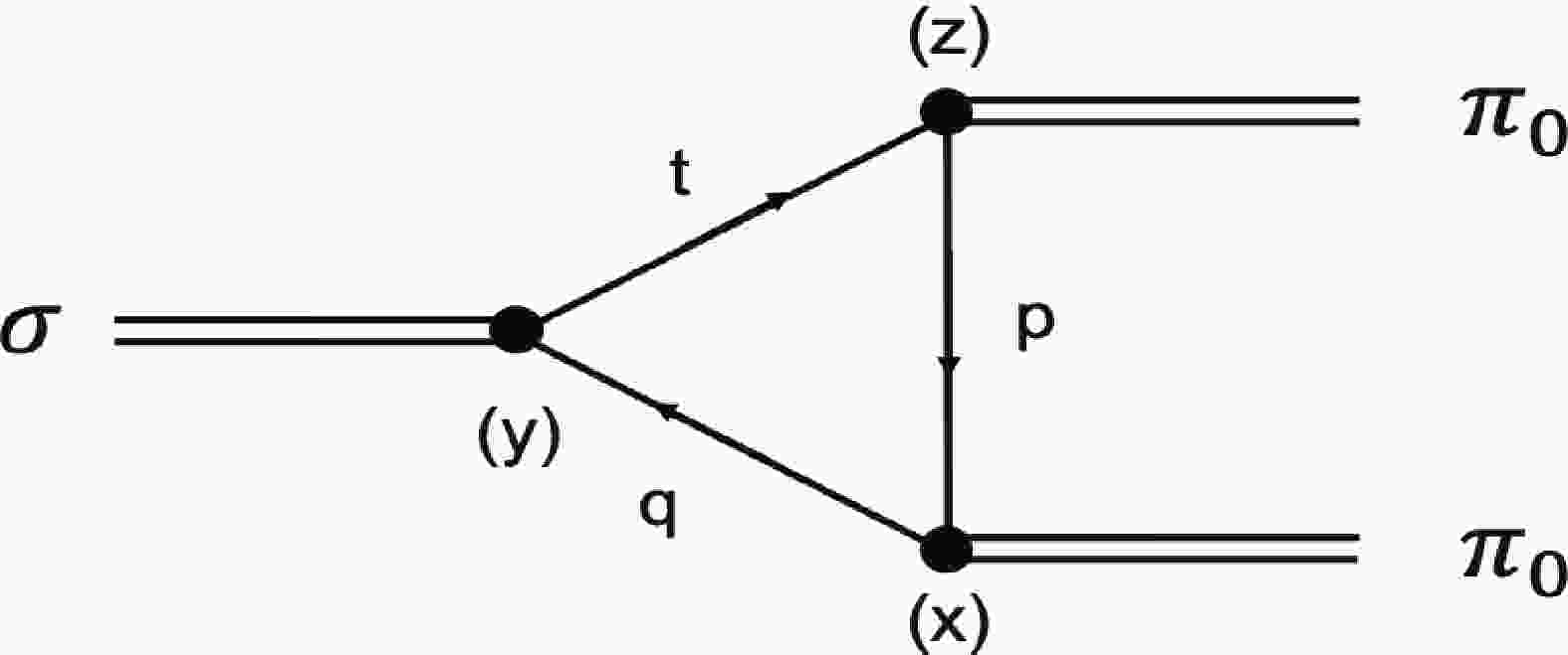
Elementary particles have the tendency to decay. For a given interaction, the larger the mass difference between the initial particles and the decay products, the faster the decay proceeds. Here we define the decay rate for $ \sigma\rightarrow \pi_{0}\pi_{0} $ at the one-loop level depicted in Fig. 1 by a Lorentz conservation matrix M [38]

Figure 1.  Feynman diagram for the process $ \sigma\rightarrow \pi_{0}\pi_{0}. $

where $ \pi_{0} $ momentum is $ |P| = \sqrt{\rm{{\dfrac{m_{\sigma}^{2}}{4}-m_{\pi_{0}}^{2}}}} $ and $ M(T,\mu) = $$ g_{\sigma}g_{\pi_{0}}^{2}A_{\sigma\pi_{0}\pi_{0}} $.

At a finite temperature and density, the decay rate of $ \sigma\rightarrow \pi\pi $ process is [39]

where $f_{\rm B}\left({m_{\sigma}}/{2}\right) = {1}/({{\rm e}^{\frac{m_{\sigma}}{2}}-1})$ is the Bose–Einstein distribution function.

σ coupling constant and π coupling constant are respectively defined by

The triangle factor $ A_{\sigma\pi_{0}\pi_{0}} $ is defined by

The vertex of the meson is expressed as

In Eq. (12), we have defined the propagator of meson in coordinate space. Here, we let

Then, we can obtain the triangle factor $ A_{\sigma\pi_{0}\pi_{0}} $

Normalization was carried out using the following formula [33]

and ${\rm e}^{-{\rm i}\widetilde{q}(x-y)-{\rm i}\widetilde{l}(y-z)-{\rm i}\widetilde{p}(z-x)}$ in coordinate space can be changed to $ (\bar{k},\bar{p}_{3}) $ momentum space by Fourier transform. For $ y-z\neq0 $ and $ z-x\neq0 $, the relationship of momentum conservation becomes

Finally, we have the triangle factor

where $ S = m_{\sigma}^2 $, $ |\boldsymbol{p}_{\bf{3}}| = \sqrt{m_{\sigma}^{2}/4-m_{\pi_{0}}^{2}} $, $ |\boldsymbol{q}| = \sqrt{q_{3}^{2}+2n|Q_{f}eB|} $. Since we only consider the decay process of $ \sigma\rightarrow \pi_{0}\pi_{0} $, the decay constant can be approximated as

The chiral condensate or the dynamical quark mass is controlled by the minimum of the thermodynamic potential [11, 12, 36, 40, 41]. Using the thermodynamic potential from Eq. (11), we have

In this work, our choice of parameters are $ m_{0} $ = 5 MeV, Λ = 653.3 MeV, $ G = 4.93\times10^{-6} $ $ \mathrm{MeV^{2}} $. The hard-cutoff regularization scheme is adopted to deal with the integral in our work. There are other kinds of regularization schemes, such as soft-cutoff regularization scheme and Pauli–Villars regularization scheme; one may find these methods in Ref. [42].

The diagrams of mass variation corresponding to the temperature under different external magnetic fields $ eB = 0, 2, 5, 7 m_{\pi}^{2} $ are plotted in Fig. 2. We observe that when the temperature increases, the mass of the quark decreases first slowly then sharply, and finally changes slowly after $ T = 200 $ MeV. For a fixed temperature, the quark mass gradually increases with the increase of magnetic field.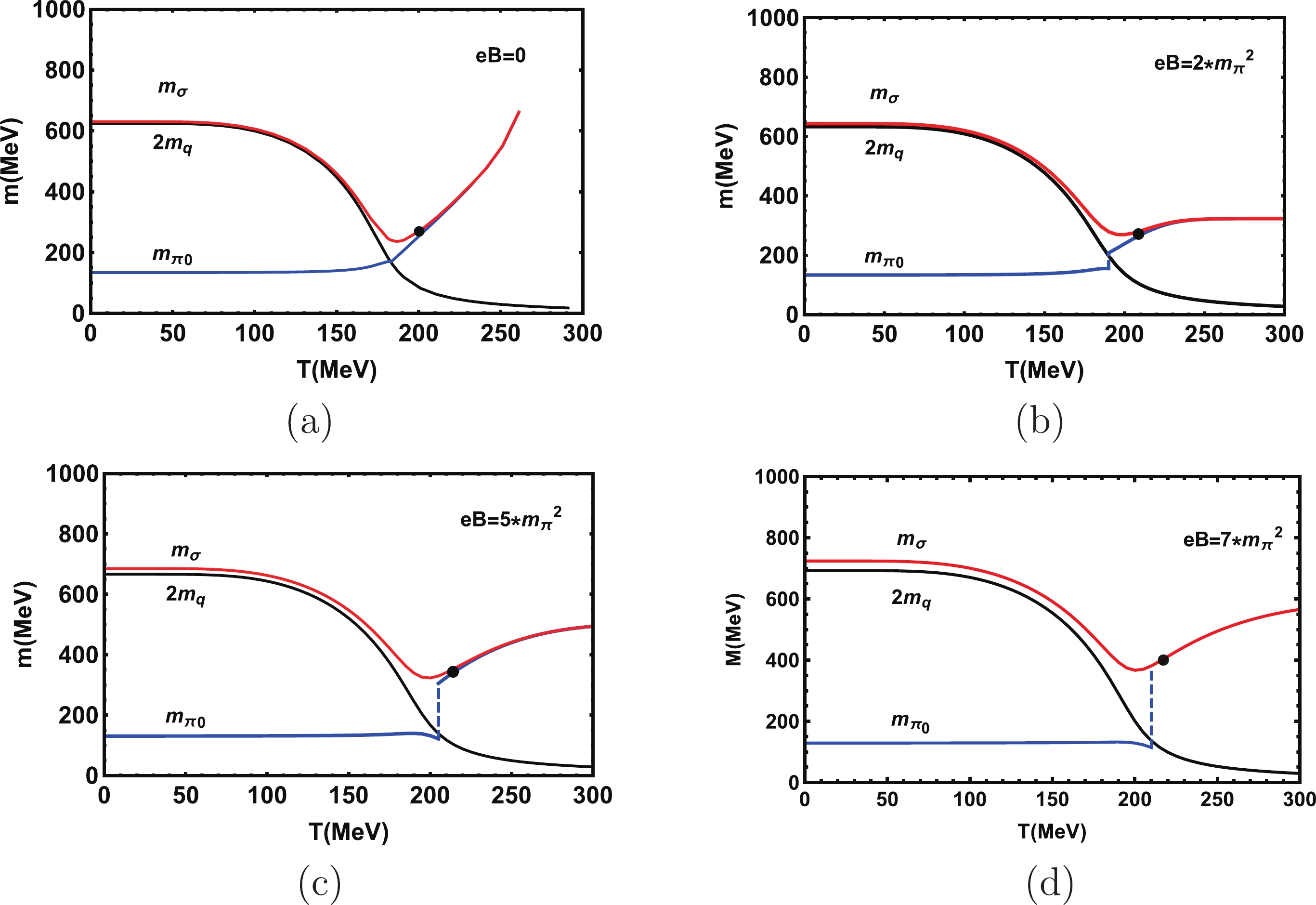

Figure 2.  (color online) Masses of quarks, σ and $ \pi_0 $ mesons at $ eB = 0, 2, 5, 7 m_{\pi}^{2} $ when $ \mu = 0 $.

Figure 2 indicates that with the increase of magnetic field, the temperature when the chiral symmetry is restored increases continuously. This temperature is the so-called critical temperature $ T_{\rm C} $. We plot black points in Fig. 2 and Fig. 3, which means that at this point, the chiral symmetry is restored. The temperature of this point is the critical temperature of the chiral phase transition $ T_{\rm C} $.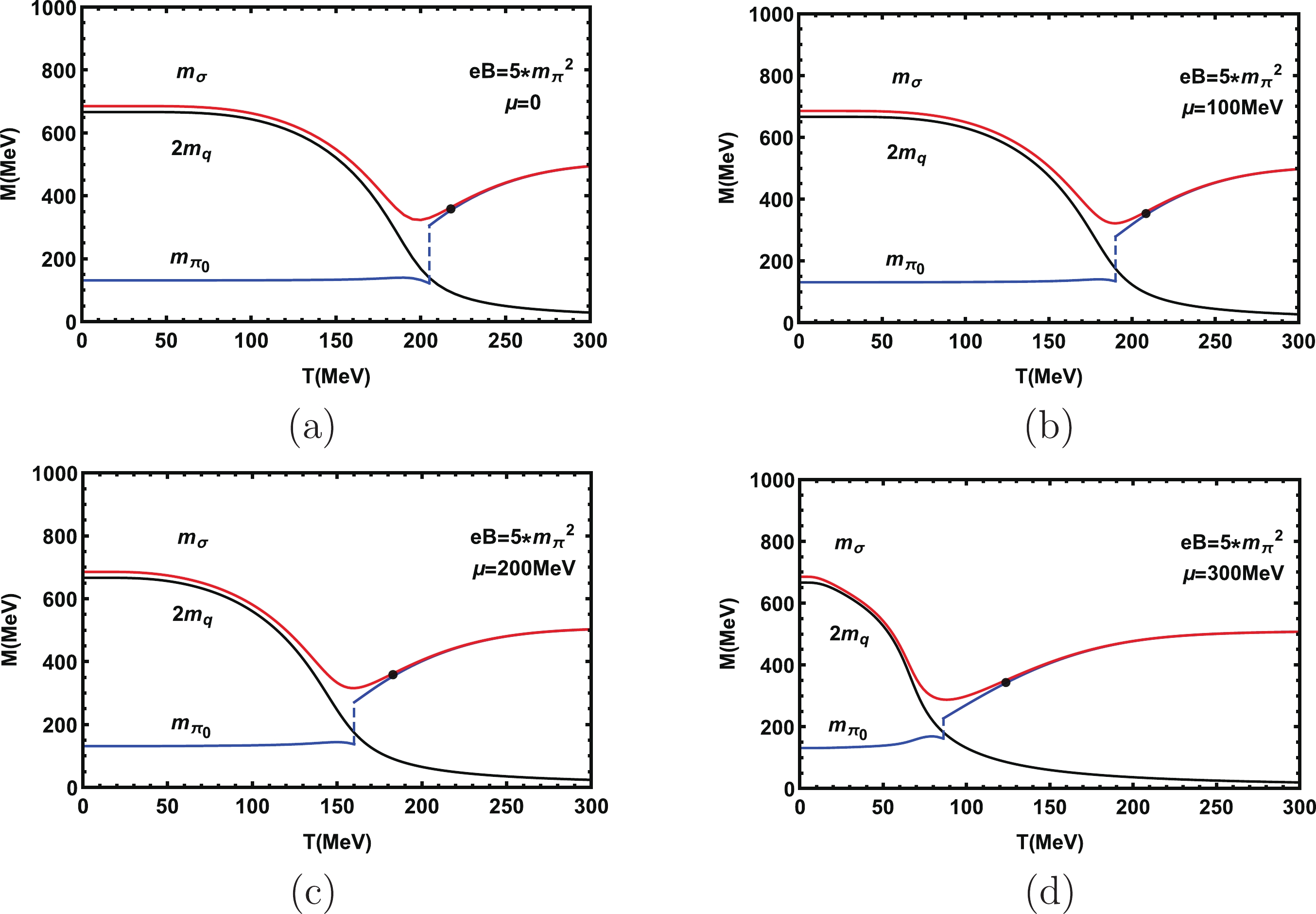

Figure 3.  (color online) Masses of quark σ and $ \pi_0 $ mesons at $ \mu = 0,100,200,300 $ MeV when $ eB = 5m_{\pi}^{2} $.

When $ m_{\pi} = 2m_{q} $, the temperature is the Mott temperature [5, 36], $ T_{\rm Mott} $, where the decay $ \pi\rightarrow $ qq is possible. When $ m_{\sigma} = 2m_{\pi} $ the temperature is the dissociation temperature, $ T_{\rm diss} $, where the $ \sigma\rightarrow \pi\pi $ decay can occur. In the chiral limit, $ T_{\rm Mott} = T_{\rm diss} = T_{\rm C} $. When $ T> T_{\rm diss} $, a σ meson can decay into two π mesons. When $ T> T_{\rm Mott} $, a π meson can decay into a pair of positive and negative quarks. When the temperature is $ T_{\rm Mott} $, there is a distinct transition in $ m_{\pi} $. There is also a distinct transition from $ m_{\sigma}>2m_{\pi} $ to $ m_{\sigma}\approx 2m_{\pi} $ at $ T_{\rm Mott} $. So we set $ T_{\rm Mott} \approx T_{\rm diss} $ in our work, and for the strong magnetic field this relation is also fulfilled.

The phase transition with temperature is a crossover, and we see that in the crossover region, the mass of the σ meson increases with the increase of the magnetic field. However in the crossover region, the mass of the $ \pi_{0} $ meson decreases slightly with the increase of magnetic field. This result agrees with that in Ref. [43]. When chiral symmetry is restored, the mass of the σ meson is degenerate with that of the $ \pi_{0} $ meson. At a finite temperature, the mass of the constituent quarks increase with the enhancement of the magnetic field, due to the fact that the external magnetic field can also cause magnetic catalysis (MC) [44-46]. In Fig. 2, we can clearly see that $ T_{\rm C} $ and $ T_{\rm Mott} $ are all increasing, and when the magnetic field is strong enough, $ T_{\rm Mott} \approx T_{\rm C} $.

Figure 3 shows the diagrams of mass change corresponding to the temperature under different chemical potentials $ \mu = 0,100,200,300 $ MeV, where we fix the magnetic filed $ eB = 5m_{\pi}^{2} $. From these figures, it is observed that when the temperature increases, the mass of the quarks decreases slowly and then decreases quickly. Finally the mass of quark changes slowly around $ T = 200,190, $$ 160, 90 $ MeV and tends to stay unchanged for different chemical potentials. For a fixed temperature, we find that as the chemical potential increases, the mass of quark gradually decreases.

When chiral symmetry is restored, the mass of the σ meson degenerates to the mass of the $ \pi_0 $ meson. Here one can clearly observe that for a fixed strong external magnetic field, with increasing chemical potential, the Mott transition temperature $ T_{\rm Mott} $ and the critical temperature $ T_{\rm C} $ for the restoration of chiral symmetry are both decreasing gradually. In the crossover region, the mass of the σ meson decreases continually with the chemical potential, while the mass of the $ \pi_0 $ increases with the chemical potential. There is still a sharp change in the mass of $ \pi_0 $ for the existence of the magnetic field.

In fact, there is some non-monotonical behavior of the pion mass near the critical temperature, which does not conflict with the chiral symmetry restoration process. This behavior was predicted by Son and Stephanov in Ref. [47] by scaling and universality arguments, and also observed later by the lattice results in Ref. [48]. This behavior is due to the interplay between the pion’s velocity and its screening mass at finite temperature. The pion’s velocity drops near $ T_{\rm C} $, while the screening mass increases with temperature.

Figure 4 shows the corresponding coupling constants $ g _ {\pi_0 qq} $ and $ g _ {\sigma qq} $ as we change the temperature. Here we fix the chemical potential $ \mu = 0 $ and the magnetic fields are $ eB = 0, 2, 5, 7 m_{\pi}^{2} $. One can see that the coupling constant becomes larger with the increase of the magnetic field. For a fixed magnetic field, the coupling constant is basically constant at low temperature, then it changes significantly around $ T = 200 $ MeV.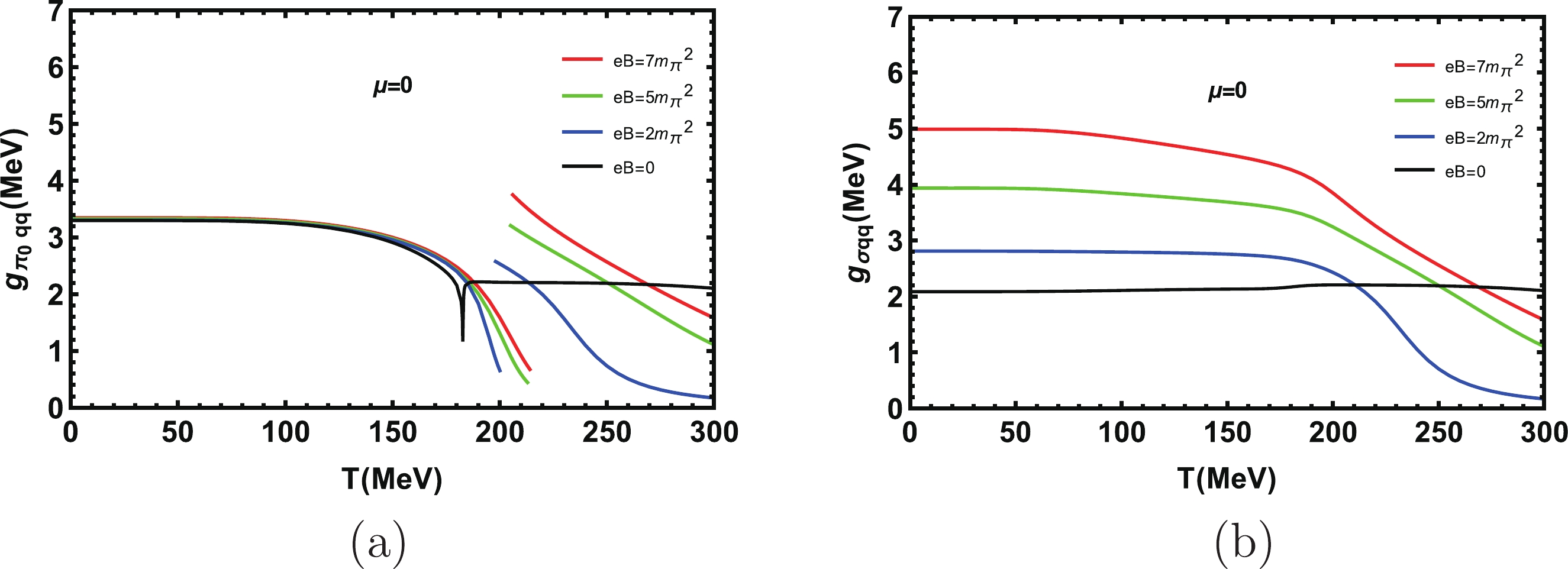

Figure 4.  (color online) Coupling constants $ g_{\pi_0 qq} $ and $ g_{\sigma qq} $ at different magnetic fields when the chemical potential $ \mu = 0 $.

In Fig. 4 (a), the corresponding coupling constant $ g _ {\pi_0 qq} $ increases slightly with the increase of magnetic field when we choose a fixed temperature. In Fig. 4 (b), the corresponding coupling constant $ g _ {\sigma qq} $ also increases with the increase of magnetic field. When it reaches $ T_{\rm Mott} $, $ g _ {\pi_0 qq} $ drops down significantly and then jumps to a high value.

Figure 5 shows the effects of the chemical potential through coupling constants $ g _ {\pi_0 qq} $ and $ g _ {\sigma qq} $. Here we fix the magnetic field $ eB = 5m_{\pi}^{2} $ and the chemical potentials are $ \mu = 0,100,200,300 $ MeV. In Fig. 5 (a), the coupling constant becomes smaller with the increase of chemical potential. For a fixed magnetic field, the coupling constant is basically constant and then changes significantly when the chemical potential is finite. One can clearly see that the critical temperature when $ g _ {\pi_0 qq} $ jumps is decreasing with the increase of chemical potential, which means adding chemical potential suppresses the decay of the $ \pi_0 $ meson. In Fig. 5 (b), the chemical potential has a significant impact on coupling constant $ g _ {\sigma qq} $, and it decreases gradually with the increase of temperature.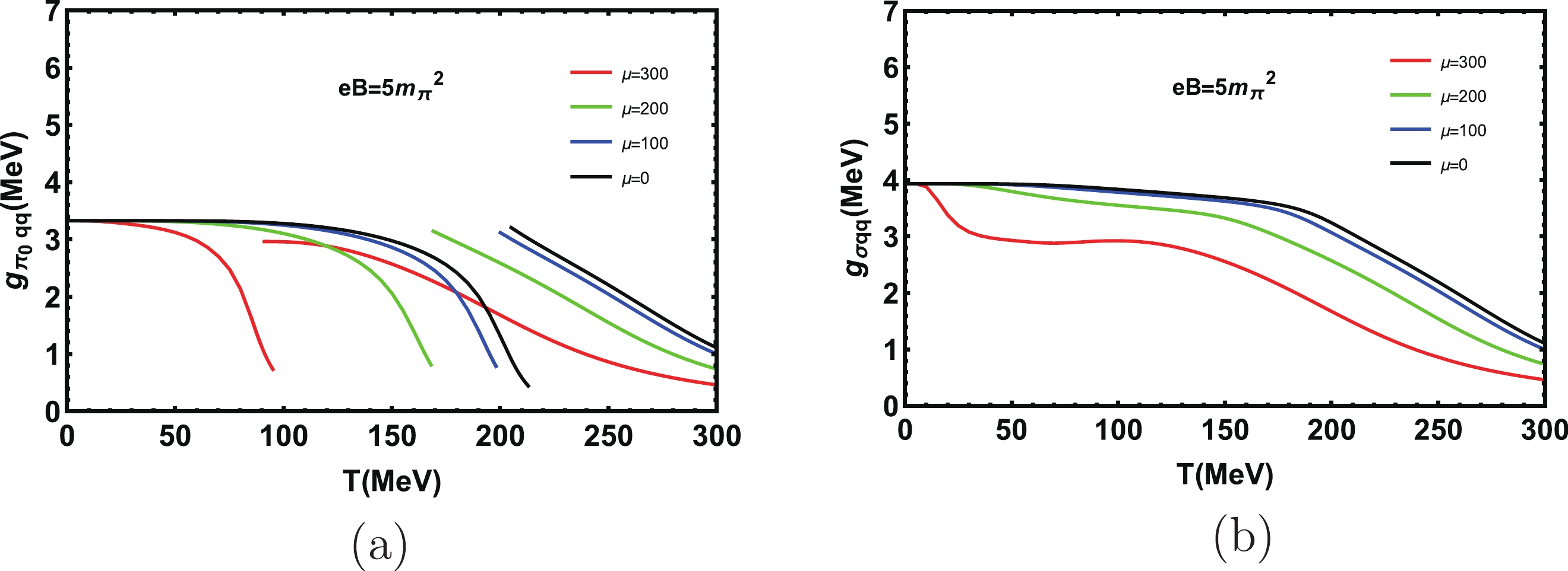

Figure 5.  (color online) Coupling constants $ g_{\pi_0 qq} $ and $ g_{\sigma qq} $ at different chemical potentials when the magnetic field $ eB = 5m_{\pi}^{2} $.

The variation of the decay width $ \Gamma _ {\sigma\rightarrow \pi_0\pi_0} $ with temperature is shown in Fig. 6 and Fig. 7. We fix the chemical potential $ \mu = 0 $ in Fig. 6, and the magnetic fields are respectively $ eB = 0, 2, 5, 7 m_{\pi}^{2} $. We find that when the magnetic field increases, the decay width increases. In Lattice QCD [49], the decay widths of $ \pi_{0} $ have been calculated. The decay constant also shows an increase with the increase of magnetic field. When $ eB = 0 $, the decay width is 84.7 MeV, and when the magnetic field is added, the decay width becomes 153.1, 310.2, and 510.6 MeV respectively. This is about 1.8 times, 3.7 times and 6.0 times of that in the case of zero magnetic field. With the increase of temperature, the decay critical point also increases from $ T = 170 $ MeV to $ T = 220 $ MeV. Finally the decay width $ \Gamma _ {\sigma\rightarrow \pi_0\pi_0} $ decreases, and goes to 0 when the temperature is around the critical point temperature. At this temperature, the decay happens rapidly and then stops.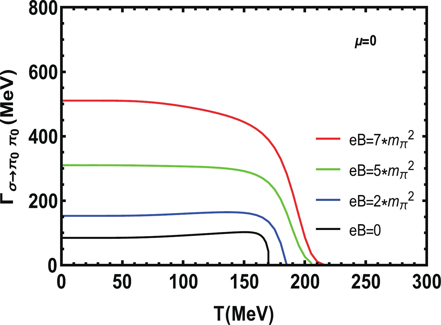

Figure 6.  (color online) Decay width $ \Gamma _{\sigma\rightarrow \pi_0\pi_0} $ at different magnetic fields when the chemical potential $ \mu = 0 $.

Figure 7.  (color online) Decay width $ \Gamma _{\sigma\rightarrow \pi_0\pi_0} $ at different chemical potentials when the magnetic field $ eB = 5m_{\pi}^{2} $.

In Fig. 7 we fix the magnetic field $ eB = 5m _ {\pi} ^ {2} $, and the chemical potentials are $ \mu = 0,100,200,300 $ MeV. One find that when the chemical potential increases, the corresponding decay width $ \Gamma _ {\sigma\rightarrow \pi_0\pi_0} $ decreases, and the decay critical points move to lower temperature. Their temperatures are respectively 210, 189, 159, 72 MeV. Near to the critical point, $ \Gamma _ {\sigma\rightarrow \pi_0\pi_0} $ suddenly changes to 0, which means the decay process stops. It is clear that the presence of the chemical potential suppresses the decay of σ meson.

Under the corresponding magnetic field in Fig. 6, the decay width increases with the increase of magnetic field, and it drops to zero at $ T_{\rm Mott} $, which reflects the restoration of chiral symmetry. Similar results on the decay widths of σ mesons at fixed chemical potential $ \mu = 0 $ can be found in Ref. [50] for the study of the decay widths of neutral π mesons decaying into photons for different neutral mesons. The increase of decay width is particularly pronounced when the magnetic field is very large. When we consider different chemical potentials and fix the external magnetic field $ eB = 5m _ {\pi} ^ {2} $ in Fig. 7, the change of $ \Gamma_{\sigma\rightarrow \pi_0\pi_0} $ looks very clear and the critical point decreases with the chemical potential.

In Ref. [5], they have considered the weak decay constant of $ \pi_{0} $ at finite temperature T, chemical potential μ and in the presence of a constant magnetic field B. In their work, they consider the decay constant of $ \pi_{0} $ at $ \mu = 0 $. In our paper, we mainly calculate the decay constant of σ with different chemical potentials and magnetic fields, that is the new point in our paper. We also calculate the mass spectra of mesons.

From all the figures, one may find that the critical temperature of $ g _ {\pi_0 qq} $, $ g _ {\sigma qq} $ and $ \Gamma _ {\sigma\rightarrow \pi_0\pi_0} $ is $ T_{\rm Mott} $, not $ T_{\rm C} $. In Refs. [27, 38, 39], $ \Gamma _ {\sigma\rightarrow \pi\pi} $ is usually associated with the chiral phase transition. In their work, the threshold temperature is $ T_{\rm diss} $ since there is no magnetic field. With the magnetic field, $ T_{\rm C} $ and $ T_{\rm Mott} $ are different — this difference is studied in Refs. [34-36]. $ T_{\rm Mott} $ is decreasing with the increase of chemical potential, which agrees with Ref. [38]. In that paper, $ \Gamma _ {\rm max} $ is first decreasing and then increasing with the increase of chemical potential, and when the chemical potential is bigger enough, it turns to zero. In our work, the change of $ \Gamma _ {\sigma\rightarrow \pi_0\pi_0} $ is different since we chose a constant magnetic field $ eB = 5m _ {\pi} ^ {2} $. With the increase of chemical potential, $ \Gamma _ {\sigma\rightarrow \pi_0\pi_0} $ is clearly decreasing.

Magnetic fields were generated in the early universe. They can influence subsequent cosmic phase transitions, which is important for particle physics in the early universe. Our results suggest that the presence of an external magnetic field "magnetizes" quarks in neutral mesons, affecting their thermodynamic properties. The existence of the magnetic field increases the critical temperature, thus increasing the symmetry breaking region and suppressing the phase transition to some extent.

From this work, we clearly see that the neutral meson is also affected by the external magnetic field, which is mainly due to the “magnetization” of the charged quarks that make up the meson, which affects the properties of the meson, such as meson mass, coupling constant, decay width and so on. Here, the effect of the magnetic field is to increase the critical temperature in the mass spectrum, thereby increasing the symmetry breaking region. At the same time, the existence of the magnetic field breaks the isospin symmetry, and the separation of quark energy levels leads to the jump in $ \pi_0 $ mass.

The effect of the chemical potential is to decrease the critical temperature in the mass spectrum. In the case of fixed strong external magnetic field $ eB = 5m_{\pi}^{2} $, with the increase of chemical potential, the masses of σ, $ \pi_0 $ and quark don't change much at low temperature, while the coupling constants and decay width all decrease. The existence of chemical potential reduces the critical temperature and accelerates the restoration of chiral symmetry. It is worth mentioning that the critical temperature of $ g _ {\pi_0 qq} $, $ g _ {\sigma qq} $ and $ \Gamma _ {\sigma\rightarrow \pi_0\pi_0} $ is $ T_{\rm Mott} $, not $ T_{\rm C} $. We know that the truly critical temperature of $ \sigma\rightarrow \pi_0\pi_0 $ should be $ T_{\rm diss} $, and $ T_{\rm Mott} \approx T_{\rm diss} $ when we consider the magnetic field in our work.

To conclude, we use SU(2) NJL model to study the decay process of $ \sigma\rightarrow \pi_0\pi_0 $, and our results show that the magnetic field will enhance the decay process while the chemical potential will reduce the decay process. In this work, a general method is used to calculate the decay constant, which can be extended to other charged mesons, such as K or ρ mesons. It can also be extended to other backgrounds, such as the 3-flavor NJL model, PNJL model and so on.