


 Abstract
 HTML
HTML Reference
 Related
 PDF
PDF


-
The detection of gravitational waves (GWs) by LIGO/VIRGO [1–5] raises people's growing interest in the study of GWs, which provides an approach to probe the early universe and new physics at high scales. A stochastic gravitational-wave background (SGWB), the preliminary target at LIGO/VIRGO and LISA [6, 7], may come from: a cosmological first-order phase transition (FOPT), cosmic strings, or inflation [8]. For some phase transition models, the GWs produced from a FOPT occurring at high temperature (far beyond the electroweak scale) cannot be reached by LISA [6, 7], nor even LIGO/VIRGO. On the other hand, cosmic strings can form when a high scale FOPT induces spontaneous symmetry breaking of a
$ U(1) $ theory in the early universe [9, 10]. In literatures, the SGWB emitted from cosmic strings has been extensively studied since cosmic strings are generic predictions of theories beyond the Standard Model, such as Grand Unified Theories [11–13], and seesaw models where a$ U(1)_{B-L} $ symmetry is spontaneously broken [14-16].In this work, we intend to investigate the scenario where the scale of the FOPT is far beyond the capacity of current and future GW detectors. We study the SGWB from cosmic strings formed after spontaneous symmetry breaking of a local U(1) driven by a FOPT. We consider Nambu–Goto strings and remind readers that the loop-production efficiency
$C_{\rm eff}$ obtained from Nambu-Goto simulations [17] is about four times larger than that of Abelian-Higgs simulations [18]. To see whether the Nambu–Goto approximation applied for the Abelian-Higgs theory requires classical field string lattice simulations, which is still under debate, see Refs. [18–23]. This paper is organized as follows. In section II, we introduce the phase transition model with a local$ U(1) $ symmetry. In section III, we compute the GWs produced from the FOPT and cosmic strings. Section IV is devoted to conclusions and discussions. -
The relevant Lagrangian is
$ {{\cal{L}}} = |D_\mu S|^2 - \frac{1}{4} F^\prime_{\mu\nu}F^{\prime\mu\nu} - V(S)\;, $

(1) with
$ F^\prime_{\mu\nu} $ being the field strength tensor of$ U(1)^\prime $ . The covariant derivative is$ \begin{align} D_\mu S & = \left(\partial_\mu + {\rm i} g_D A_\mu^\prime\right)S \,, \end{align} $

(2) where
$ g_D $ is the gauge coupling and$ A_\mu^\prime $ is the gauge boson of$ U(1)' $ . The tree-level scalar potential is given by$ V_\text{tree}(S) = - \mu_S^2 S^\dagger S + \frac{\lambda_S}{2} (S^\dagger S)^2\;, $

(3) where the
$ \mu_S^2 = \lambda_S v_s^2/2 $ can be obtained from the minimal condition of the potential,$ \begin{align} \; \; \frac{{\rm d}V_\text{tree}(S)}{{\rm d}s}\bigg|_{s = v_s} = 0\;. \end{align} $

(4) With the standard methodology, the phase transition can be studied with the thermal one-loop effective potential [24],
$ \begin{align} V_{\rm eff}(s,T)& = V_{\rm 0} (s)+ V_{\rm CW}(s)+V^{\rm c.t}_{1}(s)+ V_{1}^{T}(s,T)\, . \end{align} $

(5) The
$ V_{\rm 0} (s) $ is the tree-level potential for the classical scalar field,$ \begin{equation} V_{0} (s) = - \frac{\mu_s^2}{2}s^2 + \frac{\lambda_s}{8} s^4. \end{equation} $

(6) The Coleman–Weinberg contribution is given by [25]
$ \begin{align} V_{\rm CW}(s) = \sum_{i} \frac{g_{i}(-1)^{F}}{64\pi^2} m_{i}^{4}(s)\left(\mathrm{Ln}\left[ \frac{m_{i}^{2}(s)}{\mu^2} \right] - C_i\right)\, , \end{align} $

(7) where,
$ F = 0 \; (1) $ for bosons (fermions), μ is the$ \overline{\text{MS}} $ renormalization scale,$ g_{i} = \{1,3,1 \} $ for the$ s, \; A' $ ,$ G^D $ in$ U(1) $ model,$ C_i = 5/6 $ for gauge bosons and$ C_i = 3/2 $ for scalar fields and fermions. The field-dependent masses of the scalar, Goldstone, and gauge boson are$ \begin{aligned}[b] &m^2_{S}(s) = -\mu_S^2+\frac{3}{2}\lambda_S s^2 \,,\; \; \\ &m^2_{G_D}(s) = -\mu_S^2+\frac{1}{2}\lambda_S s^2 \,,\; \; \\ &m^2_{A'}(s) = g_D^2 s^2 \,. \end{aligned} $

(8) The counter terms to the potential in Eq. (7) are
$ \begin{equation} V^{\rm c.t}_{1} (s) = -\frac{\delta\mu_2^2}{2} s^{2} + \frac{\delta\lambda_2}{8}s^{4}. \end{equation} $

(9) To prevent shifts of the masses and VEVs of the scalars from their tree-level values, we impose
$ \begin{aligned}[b] \partial_{s} (V_{\rm CW}(s) + V^{\rm c.t}_{1}(s)) \bigg|_{s = v_s}& = 0\,,\\ \partial_{s} \partial_{s} (V_{\rm CW}(s) + V^{\rm c.t}_{1}(s)) \bigg|_{s = v_s}& = 0\,. \end{aligned} $

(10) The finite temperature effective potential at one-loop level is given by
$ V_{1}^{T}(s, T) = \frac{T^4}{2\pi^2}\, \sum\limits_i g_i J_{B,F}\left( \frac{ M_i^2(s)+\Pi_i(T)}{T^2}\right), $

(11) where the Debye masses are calculated as
$ \begin{aligned}[b] \Pi_{S(G)}(T) =& \left(\frac{\lambda_S}{6} + \frac{g_D^2}{4}\right) T^2 \,, \; \; \\ \Pi^L_{A'}(T) = & \frac{g_D^2}{3} T^2 \,. \end{aligned} $

(12) Here, we note that only the longitudinal mode will receive thermal correction. The functions
$ J_{B,F}(y) $ are$ \begin{array}{*{20}{l}} J_{B,F}(y) = \pm \int_0^\infty\, {\rm d}x\, x^2 \mathrm{Ln}\left[1\mp {\rm exp}\left(-\sqrt{x^2+y}\right)\right]\,, \end{array} $

(13) where the upper (lower) sign corresponds to bosonic (fermionic) contributions. The above integral
$ J_{B,F} $ can be expressed as a sum of the second kind modified Bessel functions$ K_{2} (x) $ [26],$ J_{B,F}(y) = \lim\limits_{N \to +\infty} \mp \sum\limits_{l = 1}^{N} {(\pm1)^{l} y \over l^{2}} K_{2} (\sqrt{y} l)\;. $

(14) With the thermal effective potential obtained above, one can obtain the solution of the bounce configuration (the bounce configuration of the field connects the
$ U(1)^\prime $ broken vacuum (true vacuum) and the$ U(1)^\prime $ preserving vacuum (false vacuum)) of the nucleated bubble, which is obtained by extremizing,$ S_3(T) = \int 4\pi r^2 {\rm d} r\Bigg[\frac{1}{2}\Bigg(\frac{{\rm d} \phi_b}{{\rm d}r}\Bigg)^2+V_{\rm eff}(\phi_b,T)\Bigg]\;, $

(15) after solving the equation of motion for the field
$ \phi_b $ , which satisfies the boundary conditions$ \lim\limits_{r\rightarrow \infty}\phi_b = 0\;, \quad \frac{{\rm d}\phi_b}{{\rm d} r}\bigg|_{r = 0} = 0\;. $

(16) The
$ \phi_b $ is the s field considered in this work. The nucleation temperature ($ T_n $ ) is obtained when the number of bubbles for bubble nucleation per horizon volume and per horizon time is of order unity [27–29]:$ \begin{array}{*{20}{l}} \Gamma\approx A(T){\rm e}^{-S_3/T}\sim 1\;. \end{array} $

(17) After analyzing the FOPT with the method in this section, one can obtain the phase transition temperature, the phase transition strength, and the phase transition duration that are crucial for calculating GWs produced during the FOPT. The FOPT further induces spontaneous breakdown of
$ U(1) $ and produces cosmic strings. -
We calculate the GWs from the FOPT and cosmic strings produced by the spontaneous symmetry breaking of
$ U(1) $ at high scales. -
One crucial parameter for calculating the gravitational wave is the latent heat of the FOPT normalized by the radiative energy, which is defined as [30]
$ \alpha = \frac{\Delta\rho}{\rho_R}\;. $

(18) Here,
$ \Delta \rho $ is the latent heat released from the phase transition to the energy density of the plasma background. Another crucial parameter is β characterizing the inverse time duration of the phase transition, given by$ \frac{\beta}{H_n} = T\frac{d (S_3(T)/T)}{d T}|_{T = T_n}\; . $

(19) The gravitational waves from the FOPT mainly include sound waves and MHD turbulence [30]. The sound waves created in the plasma constitute the leading source of GWs (The sub-leading source, i.e., MHD turbulence, is still uncertain [31]), and its energy density is given by
$ \begin{aligned}[b] \Omega h^2_{\rm sw}(f) =& 2.65 \times 10^{-6}(H_*\tau_{\rm sw})\left(\frac{\beta}{H}\right)^{-1} v_b \left(\frac{\kappa_\nu \alpha }{1+\alpha }\right)^2 \left(\frac{g_*}{100}\right)^{-\frac{1}{3}}\\&\times \left(\frac{f}{f_{\rm sw}}\right)^3 \left(\frac{7}{4+3 \left(f/f_{\rm sw}\right)^2}\right)^{7/2}, \end{aligned} $

(20) where
$ \tau_{\rm sw} = \rm{Min}\left[\dfrac{1}{H_*},\dfrac{R_*}{\bar{U}_f}\right] $ ,$ H_*R_* = v_b(8\pi)^{1/3}(\beta/H)^{-1} $ is included to account for the duration of the phase transition [32]. We take$ v_b = 1 $ in this study. The root-mean-square (RMS) fluid velocity can be approximated as [31, 33, 34]$ \begin{equation} \bar{U}_f^2\approx\frac{3}{4}\frac{\kappa_\nu\alpha}{1+\alpha}\;. \end{equation} $

(21) The term
$ H_*\tau_{\rm sw} $ is included to account for the suppression of the GW amplitude when the sound wave source can not last more than one Hubble time. The fraction of the latent heat transferred into plasma's kinetic energy is described by the$ \kappa_\nu $ factor, which can be obtained through hydrodynamic analysis [35]. The peak frequency is located at [33, 36, 37]$ \begin{equation} f_{\rm sw} = 1.9 \times 10^{-5} \frac{\beta}{H} \frac{1}{v_b} \frac{T_*}{100}\left({\frac{g_*}{100}}\right)^{\frac{1}{6}} {\rm Hz }\;. \end{equation} $

(22) For this study, we consider
$ T_\star\approx T_n $ . -
In this paper, we consider Nambu–Goto cosmic strings characterized solely by the string tension
$ \mu\approx 2\pi v_s^2n $ , with n being winding number [10]. Following the Kibble mechanism, the string tension can be roughly estimated as [38, 39]$ \mu\approx \frac{10^{-15}}{\rm G}\left(\frac{T_p}{10^{11}\; {\rm GeV}}\right)^2\; $

(23) for the cosmic strings produced from the FOPT, where G is Newton's constant. We take
$ T_p\approx T_n $ in this study. After formation, the string loops lose energy dominantly through the emission of gravitational waves. We calculate the relic GW energy density spectrum from cosmic string networks following Ref. [38]. The GW spectrum is$ \Omega_{\rm GW}(f) = \sum\limits_k \Omega_{\rm GW}^{(k)}(f)\; , $

(24) with k-mode being
$ \begin{aligned}[b] \Omega_{\rm GW}^{(k)}(f) =& \frac{1}{\rho_c} \frac{2k}{f} \frac{{\cal{F}}_{\alpha}\,\Gamma^{(k)}G\mu^2} {\alpha\left( \alpha+\Gamma G\mu\right)} \int_{t_F}^{t_0}d\tilde{t}\; \frac{C_{eff}(t_i^{(k)})}{t_i^{(k)\,4}} \\&\times\Bigg[\frac{a(\tilde{t})}{a(t_0)}\Bigg]^5 \Bigg[\frac{a(t^{(k)}_i)}{a(\tilde{t})}\Bigg]^3 \,\Theta(t_i^{(k)} - t_{osc})\;.\end{aligned} $

(25) Here,
$ \rho_c = 3H_0^2/8\pi G $ is the critical density, and the factor$ {\cal{F}}_{\alpha} $ characterizes the fraction of the energy released by long strings. We take$ {\cal{F}}_{\alpha} = 0.1 $ ,$ \alpha = 0.1 $ to consider the length of the string loops with a monochromatic loop distribution. The loop production efficiency$C_{\rm eff}$ is obtained after solving the Velocity-dependent One-Scale equations (VOS), with$ C_{\rm eff} = 5.4 (0.39) $ in a radiation (matter) dominated universe [38]②. The gravitational loop-emission efficiency$ \Gamma\approx50 $ [40], its Fourier modes for cusps [41] (emission rate per mode) are given by [40, 42]:$ \Gamma^{(k)} = \frac{\Gamma k^{-\frac{4}{3}}}{\displaystyle\sum_{m = 1}^{\infty} m^{-\frac{4}{3}} } \;, $

(26) with
$ \displaystyle\sum_{m = 1}^{\infty} m^{-\frac{4}{3}} \simeq 3.60 $ and$ \Gamma = \displaystyle\sum_k \Gamma^{(k)} $ . The formation time of loops of the k mode is a function of the GW emission time$ \tilde{t} $ and has the form of$ \begin{equation} t_i^{(k)}(\tilde{t},f) = \frac{1}{\alpha+\Gamma G\mu}\left[ \frac{2 k}{f}\frac{a(\tilde{t})}{a(t_0)} + \Gamma G\mu\;\tilde{t}\; \right]. \end{equation} $

(27) The long string oscillation time is
$t_{\rm osc } = {\rm Max}[t_{\rm fric},t_F]$ , where the formation time$ t_F $ of the cosmic string networks can connect with the phase transition through [38]:$ \begin{equation} \sqrt{\rho_{\rm tot}(t_F)}\equiv \mu\;, \end{equation} $

(28) with the tension μ being a function of phase transition temperature as given in Eq. (23). Here, we note that the formation of cosmic strings during the phase transition when vacuum bubble collision occurs (with different Higgs phases of bubbles respecting the geodesic rule) has been established by numerical simulations of variant groups [43–45]. The detailed dynamics of the cosmic strings' formation will be affected by bubble velocity and scalar oscillation during the phase transition (see Refs. [46–50]). We leave the detailed study to a separate work. For the phase transition case, taking into account the thermal friction effect, the cosmic string networks may reach scaling after the time
$t_{\rm fric}$ [38]. For loops of length smaller than the characteristic length, the particle production effect needs to be taken into account [38, 51]. For the case where cusps dominate the small-scale structure of loops, the high mode in Eq. (24) can be evaluated as$ \Omega_{\rm GW}^{(k)}(f) = \dfrac{\Gamma^{(k)}}{\Gamma^{(1)}}\,\Omega_{\rm GW}^{(1)}(f/k) = k^{-4/3}\,\Omega_{\rm GW}^{(1)}(f/k) $ . When$t_F > t_{\rm fric}$ , Eq. (25) reduces to the case in Ref. [52]. -
For cosmic strings, the GW spectrum at low and high frequencies is dominated by emissions in the matter-dominated and the radiation-dominated universe. The spectrum at high frequencies is flat in a wide range, which is therefore expected to be probed by complementary searches at LIGO [1, 53–55], SKA [56], EPTA [57], PPTA [58], IPTA [59], TianQin [60], Taiji [61], LISA [6], Einstein Telescope [62, 63], Cosmic Explorer [64], BBO [65] and DECIGO [66]. The CMB measurements constrain the dimensionless parameter to be
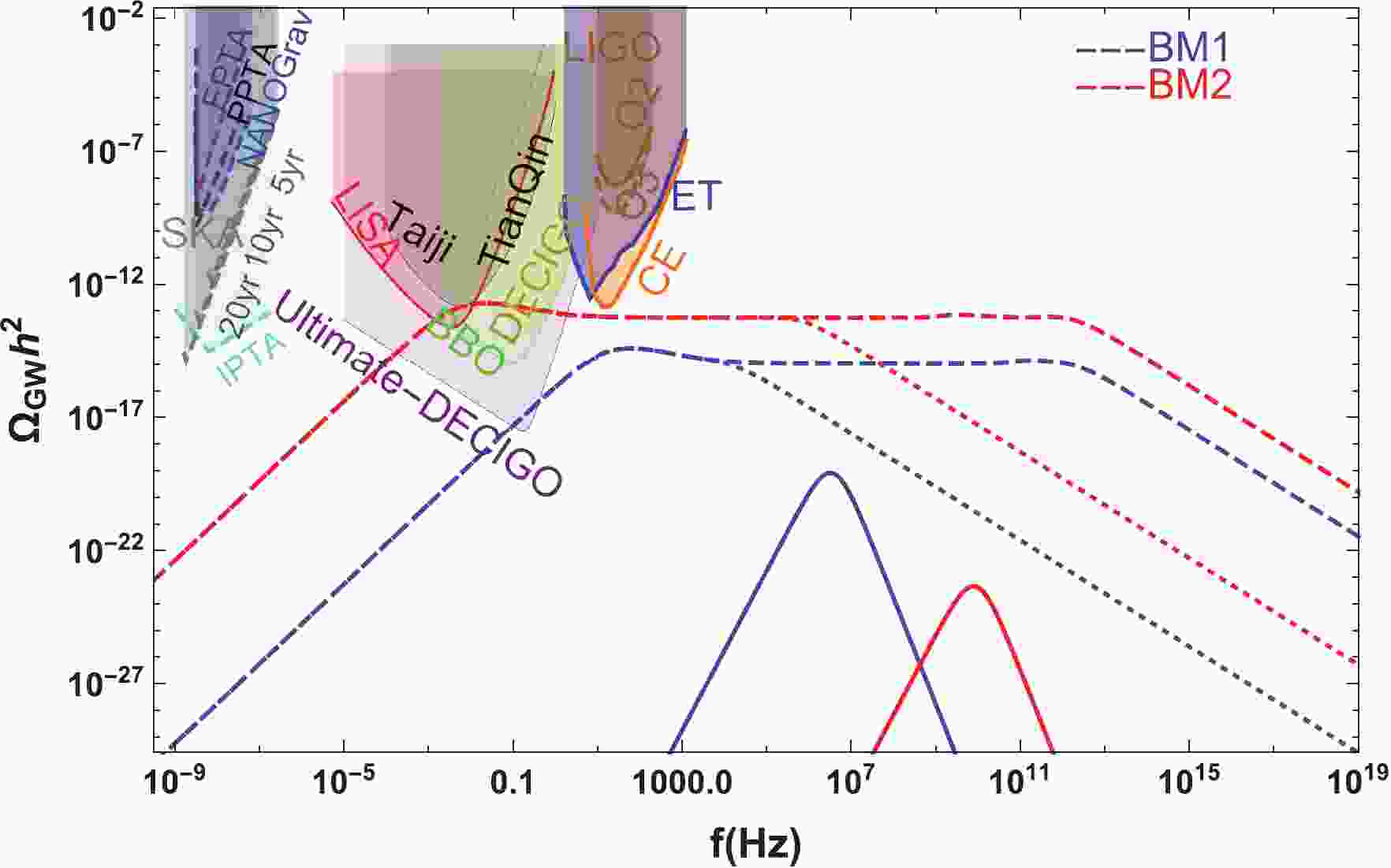
$ G\mu \leqslant 1.1 \times 10^{-7} $ [67]. The current strongest constraints come from pulsar timing array EPTA and NANOGrav:$ G\mu\leqslant 8\times10^ {-10} $ [68],$ G\mu\leqslant 5.3\times10^ {-11} $ [69]. the$ G\mu< 10^{-11} $ corresponds to$ T_n \leqslant 10^{15} $ GeV for FOPT scenarios. With Eqs. (23), (28), we found that one cannot have formation of string loops for$ T_n\geqslant {\cal{O}}(10^{11}) ~~{\rm GeV} $ . We therefore focus on cosmic strings formed after the FOPT with$ T_n\leqslant {\cal{O}}(10^{11}) ~~{\rm GeV} $ .Firstly, Ref. [7] shows that LISA is capable of probing cosmic strings with tensions
$ G\mu\geqslant {\cal{O}}(10^{-17}) $ when the Nambu–Goto strings with the average loop size at formation have$ \alpha\approx 0.1 $ , which corresponds to a phase transition temperature$ T_n\geqslant 10^{10} $ GeV as indicated by Eq. (23). To show the sensitivity of LISA to GWs from cosmic strings and FOPT for the situation, in Fig. 1 we present the GW spectra by adopting the benchmark of BM2 in Table 1 (where$ T_n = 1.332\times 10^{10} $ GeV). We found that the GW from the FOPT is beyond the capacities of current and future GW detectors shown in the figure, while LISA, BBO, and DECIGO can probe the GW from the cosmic strings formed after the FOPT. We also present the sensitivity of Ultimate-DECIGO to GWs from cosmic strings formed after the FOPT for BM1 of Table 1 (with a$ T_n\geqslant {\cal{O}}(10^8) $ GeV). The cut-off effects shown in the spectrum of the GWs from cosmic strings are beyond the ranges of all detectors presented in the figure. The cut-offs at the higher frequencies (dashed lines) represent the formation times of string loops, which correspond to the phase transition temperatures of the FOPT. The cut-offs at the lower frequencies (dotted lines) are due to the impact of thermal friction, which reflects the interaction between strings and particles of the thermal plasma; for detail, see Ref. [38].
Figure 1. (color online) Gravitational wave spectra. Gravitational waves from cosmic strings are shown by dashed lines, the dotted lines represent the cut-off due to thermal friction, and gravitational waves from FOPT are shown by solid lines.
Benchmark points λ $ g_D $ 

$ v_s $ /GeV

$ v_n $ /GeV

$ T_n $ /GeV

α $ \beta/H_n $ 

$\rm BM_1$ 

$ 0.096 $ 

$ 1.459 $ 

$ 1.056\times 10^{9} $ 

$ 1.051\times 10^{9} $ 

$ 2.545\times 10^{8} $ 

$ 0.031 $ 

$ 6.467\times 10^{4} $ 

$\rm BM_2$ 

$ 0.822 $ 

$ 2.164 $ 

$ 1.921\times 10^{10} $ 

$ 1.774\times 10^{10} $ 

$ 1.332\times 10^{10} $ 

$ 0.015 $ 

$ 3.005\times 10^{6} $ 

Table 1. The two benchmark points shown in Fig. 1.
-
In this paper, we study the SGWB from cosmic strings that are formed after the FOPT at high scales. Utilizing a local
$ U(1)^\prime $ theory, we found that the cosmic strings can form when the phase transition temperature$ T_n\leqslant 10^{11} $ GeV. We found that the SGWB from the high scales phase transition under study cannot be reached by any current or planned GW detectors. The SGWB from the cosmic strings can be detected by space-based interferometers when phase transition temperature$ {\cal{O}}(10^8) $ GeV$ \leqslant T_n \leqslant {\cal{O}}(10^{11}) $ GeV. It is found that LISA is able to probe the GWs from the cosmic strings when the phase transition occurs at the temperature of:$ {\cal{O}}(10^{10}) $ GeV$ \leqslant T_n \leqslant {\cal{O}}(10^{11}) $ GeV. Therefore, our study shows that the probe of cosmic strings at GW detectors may serve as a probe of FOPTs occurring at high scales.We didn't consider the supercooling phase transition, where one may have slightly stronger GWs from the FOPT [34, 70, 71]. However, since the string tension is determined by the phase transition temperature, our study on the SGWB from cosmic strings still applies.
-
We are grateful to Alexander Vilenkin, Yanou Cui, Marek Lewicki, David E. Morrissey, James D. Wells, Daniel G. Figueroa, Ruth Durrer, David Weir, Jeff A. Dror, Yann Gouttenoire, Luca Visinelli, Nicklas Ramberg, Eric Madge, Huai-Ke Guo, Yue Zhao, and Ye-Ling Zhou for helpful communications and discussions.
Gravitational waves from cosmic strings after a first-order phase transition
- Received Date: 2021-11-09
- Available Online: 2022-04-15
Abstract: We study the possibility of probing high scale phase transitions that are inaccessible by LIGO. Our study shows that the stochastic gravitational-wave radiation from cosmic strings that are formed after the first-order phase transition can be detected by space-based interferometers when the phase transition temperature is


 DownLoad: