


 Abstract
 HTML
HTML Reference
 Related
 PDF
PDF


-
The LHAASO team will also perform interesting studies, both for basic science and for applications, of solar and heliospheric effects on the cosmic ray flux. These are basically the effects of the solar wind and solar storms, and as such they are directly related to so-called "space weather" effects of the solar wind and solar storms on human activity. LHAASO will obtain unique information on the magnetic fields between the Sun and the Earth, which are moving toward Earth with the solar wind. Indeed, LHAASO will obtain information on the direction of the interplanetary magnetic field, which is a key determinant of whether a solar wind disturbance or solar storm will result in reconnection with Earth's magnetic field and trigger a geomagnetic storm. Thus the real-time data from LHAASO will complement other information for space weather forecasting. In addition, LHAASO will perform numerous other studies of solar, heliospheric, and geomagnetic effects on cosmic rays.
-
Solar storms and the solar wind, as they propagate throughout the heliosphere, have a profound effect on cosmic rays at GeV-range energy, leading to a wide variety of signatures in cosmic ray flux variations with time. These have mostly been studied with detection thresholds up to 10 GeV or slightly higher. With its tremendous count rate at high altitude, LHAASO will obtain sufficient statistics to open the gateway to study many of these phenomena at even higher energy, thus providing new information on these processes. In addition, some phenomena, such as the Sun shadow and Moon shadow, are more profitably examined at TeV energies, where LHAASO will again provide improved statistical accuracy. In studies of time variations, improved statistics allow the possibility of studies at finer time resolution. As we shall describe, LHAASO can even provide useful real–time data for space weather forecasting.
LHAASO will generate two types of data of interest for solar-heliospheric studies: reconstructed shower rates (as a function of energy, direction, and time) and scaler rates (as a function of threshold energy and time).
One of the design goals of LHAASO is to reconstruct showers for gamma rays and cosmic rays down to tens of GeV in energy. Thus reconstructed showers with information on the arrival direction of primary cosmic rays will allow the study of the Sun and Moon shadows over a wider energy range, as well as loss-cone anisotropy to provide advance warning of the arrival of some interplanetary shocks, which can lead to various space weather effects. Directional shower data down to tens of GeV will allow a better determination of the diurnal anisotropy as well [1].
LHAASO will also produce scaler rates (also referred to as the single particle technique or SPT), in which the shower is not reconstructed but count rates are collected for various threshold numbers of "hits" in the detectors. The rate for each threshold has a different response as a function of the primary cosmic ray energy. This opens a possibility to obtain higher rates (and better time resolution) and information on lower energies below the shower reconstruction threshold. (Note, however, that the LHAASO site has a cutoff rigidity of about 13 GeV for protons, so cosmic rays below this energy cannot be examined.) Examples of existing detectors that have examined scaler rates are ARGO-YBJ [2–4] and Auger [5]. To make proper use of scaler rates, we will need to correct for environmental factors. This will require careful monitoring of the weather, atmospheric conditions, and local temperature at each detector.
-
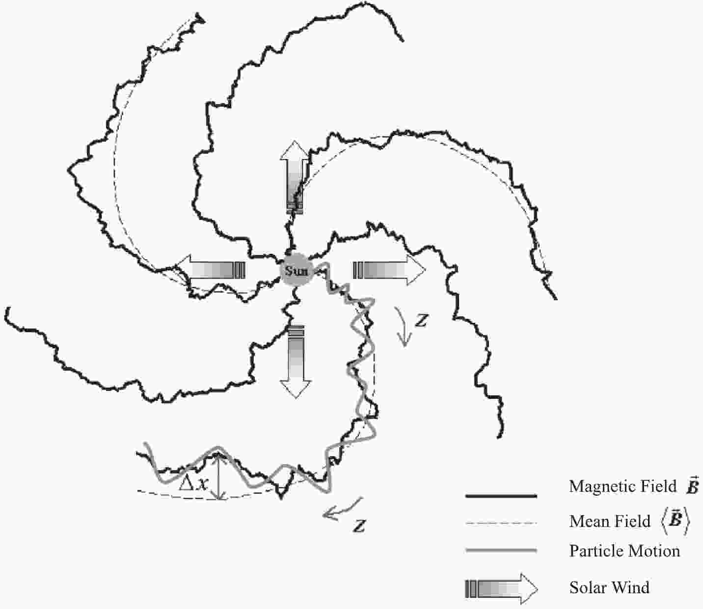
The shadow of the Sun in TeV-range cosmic rays directly relates to solar-terrestrial relations, i.e., how solar phenomena affect the Earth and its immediate environment. The solar wind is a radial flow of plasma out from the Sun at supersonic speeds, which comes out at all times and in all directions (Figure 1). The solar wind drags out the complex coronal magnetic field to become the interplanetary magnetic field. However, both the solar wind plasma flow and the interplanetary magnetic field are highly turbulent, and magnetic fluctuation amplitudes are of the same order as the mean field. Roughly speaking, an interplanetary field line connects parcels of plasma that came from the same region of the solar corona, and because of the solar rotation, its shape is curved into an Archimedean spiral. The solar wind plasma and magnetic field usually take about 4 days to come from the Sun to the Earth.

Figure 1. (color online) Illustration of the solar wind and interplanetary magnetic field. The solar wind is emitted radially from the Sun in all directions at all times. The spiral magnetic field lines connect plasma that originated from the same location on the rotating solar surface. Note that the turbulent magnetic field lines (solid lines) do not coincide with the mean magnetic field lines (dashed lines). The Earth might be located near the bottom of the figure [6].
The arrival direction distribution from shower reconstruction of TeV-range cosmic ray trajectories shows deficits corresponding to the locations of the Sun and Moon [7]. The solar, interplanetary, and terrestrial magnetic fields deflect the particle paths and shift the shadow of the Sun from its actual location, as first reported by the Tibet AS experiment [8]. In other words, the measured deflection of cosmic rays is a cumulative effect of magnetic fields along the whole path from the Sun to the Earth.
This experiment also observed the effect of the interplanetary magnetic field (IMF) [9, 10] a solar cycle variation [11], and coronal mass ejections [12], and evaluated the effects of two coronal magnetic field models [13]: the potential field source surface (PFSS) [14, 15] and current sheet source (CSSS) models [16, 17]. Further experiments of LHAASO can also be used to evaluate more advanced coronal magnetic field models, e.g., the nonlinear force-free field (NLFFF), magneto-hydrostatic (MHS), and magneto-hydrodynamic (MHD) magnetic field models [18]. On the other hand, the electromagnetic fields investigation (FIELDS) aboard the Parker Solar Probe (PSP) offers the first-ever magnetic field measurements in the interplanetary space as close as 10 solar radii from the Sun. Together with the solar wind speed measurements by the Solar Wind Electrons Alphas and Protons Investigation (SWEAP), PSP can add further valuable observational constraints to the aforementioned magnetic field models [19]. The recently launched Solar Orbiter mission is equipped with in-situ magnetic field and solar wind measurements in interplanetary space as well. Together with the measurements close to Earth, the optimal magnetic field models can hopefully be obtained.
-
Solar activity, including the likelihood of solar storms and space weather effects on human activity, is positively associated with the sunspot number, which varies with a cycle of roughly 11 years, known as the "sunspot cycle" or "solar cycle" (see Figure 2). The ARGO-YBJ collaboration also found that the deficit of cosmic ray flux in the Sun shadow is reduced with increasing solar activity [22], as shown in Figure 3. To understand the shadow effect, it is useful to imagine trajectories of antiparticles traveling backward from Earth to intersect the Sun's surface, which are equivalent to the forward trajectories that are blocked by the Sun, causing the shadow. One possible explanation of the weaker Sun shadow with increasing solar activity is that if the solar coronal magnetic fields are very irregularly distributed, the cosmic ray deflections could be so randomized that backward trajectories over a wider range of angles can intersect the Sun. Ref. [22] considers another mechanism: variation and frequent reversals of the IMF during each three-month observation period causes a superposition of Sun shadows with different shifts and leads to an observed shadow that is wider and weaker.
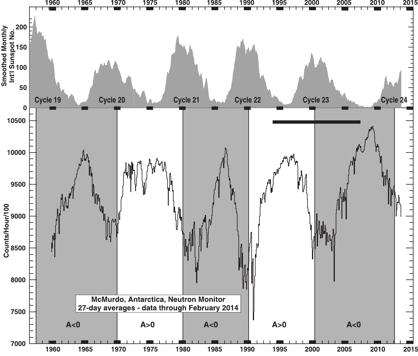
Figure 2. (color online) Smoothed monthly international Sunspot number (using 5-month boxcar smoothing) and McMurdo neutron monitor count rate as a function of time. The long-term drift at McMurdo has been corrected following [20]. A neutron monitor count rate indicates the Galactic cosmic ray flux, which undergoes "solar modulation" in association with solar activity. Solar modulation includes dramatic 11-year variations with the sunspot cycle, and a 22-year variation with the solar magnetic cycle, seen here in changes in the solar modulation pattern between positive (A>0) and negative (A<0) magnetic polarity [21].
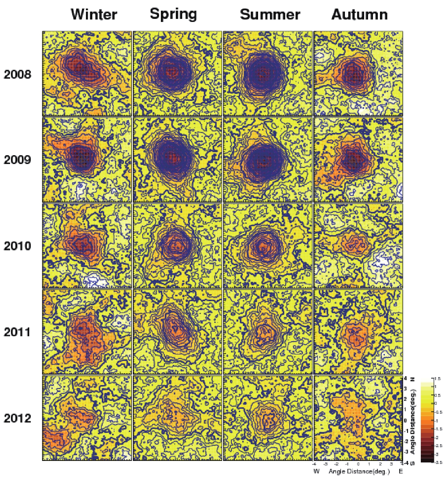
Figure 3. (color online) Seasonal variation in the Sun shadow observed by the ARGO-YBJ experiment in cosmic rays at median energy 5 TeV. The observation period for each map is one astronomical season in the Northern Hemisphere. The smoothing radius is 1.2
$^\circ$ and the pixels are 0.1$^\circ$ $\times$ 0.1$^\circ$ . Each map shows the fractional change in the cosmic ray flux (color scale) and the statistical significance of the change (contours). Each contour represents an integral value of the significance (in units of the standard deviation), with darker contours every 5 units. Maps for the Spring and Summer seasons show stronger significance because the Sun was higher in the sky at the ARGO-YBJ site in Tibet. The fractional change suddenly weakened in Spring 2010, in association with a sudden increase in IMF variability, whereas the sunspot number and some other generic indicators of solar activity started to increase rapidly only in Spring 2011 [22]. -
The Sun produces energetic particles due to occasional sudden explosions at its surface, called solar storms, which can accelerate particles to relativistic energies (ions up to tens of GeV, electrons up to tens of MeV) for durations up to about an hour. Furthermore, a type of storm called a coronal mass ejection (CME) can drive an interplanetary shock that accelerates ions up to tens of MeV (called "energetic storm particles") over several days. The particles due to solar storms, collectively called solar energetic particles (SEPs), pose a radiation hazard to astronauts and high-altitude passenger aircraft for short but unpredictable time periods, as well as damaging expensive satellites and spacecraft (at least fifteen have been disabled by solar storms to date). Strong UV and X-ray fluxes lead to increased ionospheric ionization and disturb human communications and navigation signals. The shock and CME carry particularly strong magnetic fields, and they can significantly disturb the Earth's magnetosphere. In particular, a strong southward magnetic field can lead to magnetic reconnection and a strong inflow of solar wind plasma and energetic particles into the Earth's magnetosphere, which can also damage satellites. A disturbed magnetosphere can lead to geomagnetically induced currents and power outages. All these effects on human activity can collectively be called "space weather" effects.
There is great practical interest in space weather prediction, but current prediction capabilities are very limited. The situation is analogous to long-term weather forecasting some decades ago, when the best results were based on prior experience and qualitative concepts. For modern space weather forecasting, even after a CME has been observed at the Sun, it remains difficult to predict when an interplanetary shock and CME will arrive at Earth (which can be
$ \sim $ 1-4 days, depending on the CME speed), and very difficult to measure or infer the orientation of the magnetic field of the CME; a southward field would result in particularly strong space weather effects.The ARGO-YBJ experiment first used the Sun shadow displacement in the south-north direction to measure the intensity of the magnetic field between the solar wind from the Sun to the Earth, during the previous period of minimum solar activity [23] (see also [10]). This capability could also be used to determine the mean magnetic field orientation between the Sun and Earth, before the field arrives at Earth. At present, the best reported time resolution for Sun shadows – that of the ARGO-YBJ group [22] – is three months, which is not of practical use for space weather forecasting. However, because of its much greater size, LHAASO is expected to produce a statistically meaningful Sun shadow every 1-2 days. This is then directly useful for space weather forecasting. For example, a Sun shadow determined for time t can be compared with the previous Sun shadow, observed 1-2 days earlier, and the difference is due to new magnetic fields that have emerged from the Sun minus old fields that have passed the Earth. When making use of in situ spacecraft observations of the interplanetary magnetic field, we can determine the new magnetic field that emerged from the Sun during that time interval. Then we can infer the orientation of the magnetic field that will pass by Earth in the next few days, including whether the field will have a strong southward component. This will be important information to complement existing data for space weather forecasting. On the other hand, we can perform state-of-the-art MHD simulations of the CME propagation in solar-terrestrial space, e.g., with the SWMF code, in the solar corona (SC) and inner heliosphere (IH) regimes to derive the evolution of the interplanetary magnetic field associated with the CME transition [24]. A next step is to include the CME disturbed solar-terrestrial magnetic field in order to simulate the resulting Sun shadow. The interlink between CME simulations and Sun shadow simulations can shed light on the capability of the Sun shadow as an approach for space weather forecasting.
-
The loss cone anisotropy is another type of measurement of Galactic cosmic rays that is directly relevant to space weather forecasting because it could provide advance warning of the arrival of an interplanetary shock, and could also indicate an expected time of arrival. This would be useful because a shock arrival often coincides with a sudden storm commencement as determined by ground-based geomagnetic observatories, i.e., it marks the start of a geomagnetic storm and the associated space weather effects.
The loss cone anisotropy is a decrease in GeV-range cosmic ray density in only a narrow range of directions, found within 1-2 days before the arrival of an interplanetary shock at Earth. Note that after the shock arrives, there is a decrease in the cosmic ray flux from all directions, known as a Forbush decrease [25], because the high plasma speed and strong magnetic fields inhibit access of cosmic rays to the region downstream of the shock. Now the Forbush decrease itself is not directly useful for space weather forecasting because it arrives after the shock, i.e., after the geomagnetic storm commencement. However, the "loss cone" is a range of angles close to the interplanetary magnetic field direction toward the shock, and particles from these directions came from downstream of the shock where the particle flux is lower. Hence a loss cone anisotropy is an indicator of the approach of an interplanetary shock.
A loss cone anisotropy was first reported in data from neutron monitors, in 1992 [26]. Later there were numerous other reports of loss cone decreases in neutron monitor data, as well as an enhancement of cosmic ray flux in a ring of directions surrounding the loss cone, which was attributed to reflection from the shock. The first theoretical description of the anisotropy and its spatial distribution was provided by [27]. Further computer simulations [28] provided a basis for comparison, so that an observed loss cone angle can be used to infer the shock-field angle. That work has been used to parameterize more recent determinations of loss cone shock precursors by the Global Muon Detector Network (GMDN) with fine directional resolution [29, 30].
LHAASO's reconstructed showers will have excellent directional precision and a huge count rate, over a cosmic ray energy range similar to that of GMDN, so LHAASO will provide improved measurements of the loss cone anisotropy, including a possible discovery of fine directional structure beyond the axisymmetric fits performed with presently available data. This could be used in real time to provide advance warning of impending shock arrivals and geomagnetic storm onsets. According to [28], in this energy range the loss cone feature can provide warning up to 12 hours in advance. With a single detector facility, loss cone precursors can be seen when the interplanetary magnetic field direction rotates into view, which will often but not always occur during that 12-hour window. Therefore, a more comprehensive warning system could be obtained by teaming up with GMDN, other air shower arrays, or neutron monitors worldwide to continuously monitor loss cone features along the interplanetary magnetic field direction.
-
There are also transient cosmic ray flux and anisotropy variations due to major solar storms. The main effect is the so-called Forbush decrease [25]. The first stage of the decrease occurs at a shock driven by a CME. There may be a second stage associated with the arrival of the CME ejecta, with a further decrease that lasts while the ejecta pass the observer [31]. After that, the flux returns to normal over the next few days. It is common to observe interesting anisotropy patterns during a Forbush decrease, often indicating interesting directional distributions of particles following the magnetic structures of the CME. The mechanism for the Forbush decrease is not clear, and the energy distribution of the decrease could provide important clues.
Air shower arrays can play a role by determining the Forbush decrease at high energies, where the energy and time dependence have not been systematically studied. For example, the ARGO-YBJ Collaboration reported the detection of a Forbush decrease on 2005 Jan 18 [32]. LHAASO could provide a great increase in statistics, though it will be necessary to understand and correct for environmental effects on the count rate as a function of time. Together with time-dependent cosmic-ray transport models with a three-dimensional diffusion barrier [33], we can simulate the Forbush-decrease events in different rigidity ranges and for different particle species to understand their possible mechanisms.
-
The longest–period cosmic ray variations that are directly measured are related to the 11-year sunspot cycle and the 22-year solar magnetic cycle. The number of sunspots typically varies over 11 years. There were sunspot maxima in 1989, 2000, and 2014, and sunspot minima in 1996, 2008, and 2019. Because magnetic fields and solar storms are concentrated near sunspots, numerous solar phenomena vary with the solar cycle. They do not precisely depend on the sunspot number, so we tend to speak of "solar maximum" as a period of several years around solar maximum, and "solar minimum" as a period of several years with very few sunspots. Because of the higher solar wind speed (on average) and stronger magnetic fields during solar maximum, the transport of cosmic rays into the inner heliosphere is inhibited. Thus the flux of cosmic rays is observed to have an inverse association with the sunspot number, with the most cosmic rays during solar minimum, and the fewest during solar maximum [34]. The amplitude of variation is
$ \sim 30 $ % at an energy of 1 GeV. This roughly 11-year variation is called the solar modulation of cosmic rays (Figure 2).The Sun's magnetic field is much more complex than the Earth's, and magnetic fields are highly concentrated at the sunspots, typically directed outward at one and inward at another. Nevertheless, there is an overall preponderance of one polarity on one hemisphere and the opposite polarity on the other. Every 11 years or so, at solar maximum, there is a magnetic reversal in which the preponderance reverses sign. Therefore, a complete magnetic cycle requires two sunspot cycles, i.e., about 22 years. Charged particle orbits undergo drift motions that depend on the charge sign and the sign of the magnetic field. The drifts therefore reverse every 11 years and repeat every 22 years. The same holds for the effect of magnetic helicity on the particle scattering. Therefore, there is also a roughly 22-year cosmic ray flux variation corresponding to the solar magnetic cycle [35]. In other words, 11-year periods with opposite magnetic polarity exhibit distinct cosmic ray variations. These effects are associated with a variety of interesting phenomena, such as guiding center drifts, cosmic ray gradients with helio-latitude, particle charge sign dependence, and changing diffusion coefficients [36–38]. These phenomena depend on the sign of
$ qA $ , where q is the particle charge and A is the solar magnetic polarity.With stable, long-term operation, LHAASO will provide important information to further explore solar modulation as a function of energy and time, if its threshold can be reduced to
$ \lesssim50 $ GeV. There may even be sufficient compositional information to discern the individual modulation of protons and alpha particles as a function of energy throughout the solar cycle. This is information that is not available from traditional ground-based observatories of GeV-range cosmic rays, such as neutron monitors and muon detectors. -
Roughly speaking, a faster solar wind speed can inhibit the entry of cosmic rays to the inner heliosphere, and is typically associated with a reduced cosmic ray flux. Thus co-rotational variations in solar wind speed (which rotate with the Sun) are associated with well-known "synodic" or "27 day variations" in the cosmic ray flux [39], which have sometimes been called "recurrent Forbush decreases." It frequently happens that a region of the solar corona that produces fast solar wind, e.g., a coronal hole, lies eastward of a region that produces slow solar wind. Then as the Sun rotates, the source region of fast solar wind moves underneath the region where slow solar wind came out previously, and the fast solar wind will collide with the slow solar wind that lies in front of it. Such a collision region is called a co-rotating interaction region (CIR), The CIR also has a spiral shape, and it represents a region where solar wind is suddenly compressed by the collision. An observer near Earth sees the solar wind speed suddenly increase when the faster solar wind arrives.
It is common to see the cosmic ray flux suddenly decrease at the time of the CIR, either as part of the inverse relationship with solar wind speed or because the compressed plasma and increased magnetic field serve as a barrier to hinder access to cosmic rays (see Figure 4, and note the reversed time axis). These jumps are a key component of the 27-day variations in cosmic ray flux with solar rotation. Note that CIRs also cause geomagnetic storms and space weather effects, so there is some practical interest in what cosmic rays can tell us about the physical properties of CIRs. LHAASO data could provide further insight, especially with regard to the energy dependence, which may allow us to clarify and quantify the association with solar wind parameters. It will be challenging for LHAASO to reduce its threshold to sufficiently low energy to observe cosmic ray flux variations, but it is perhaps more likely for 27-day effects to be observed in the solar diurnal anisotropy (see below). And promisingly, future coordinated observations by solar space missions, e.g., NASA’s Parker Solar Probe, ESA’s Solar Orbiter and the Chinese Advanced Space-based Solar Observatory will provide better solar wind parameters and better Carrington maps of photospheric magnetic field to calculate interplanetary magnetic field.

Figure 4. (color online) Reversed time plots in day of year (DOY) for Carrington (solar) rotation 2071 (between 2008 June 12 and 2008 July 10). Top panel: Synoptic map of the solar corona as observed by the EUVI–A imager in the Fe XII 195–Å bandpass. Upper three graphs: Data of the diurnal anisotropy and flux of Galactic cosmic rays (GCRs) as measured by the Princess Sirindhorn Neutron Monitor at Doi Inthanon, Thailand. Lower graphs: Hourly interplanetary plasma parameters from the ACE and OMNIWeb databases in GSE coordinates. When the high speed solar wind streams pass the Earth they reduce the cosmic ray flux. After the rapid solar wind speed increase of DOY 177, there was a strong, long–lasting enhancement in the diurnal anisotropy of GCRs. This is attributed to an extra
${\bf B}\times\nabla n$ anisotropy with a latitudinal gradient in association with the coronal hole (dark region) morphology [40]. -
The sidereal anisotropy (also called the sidereal diurnal anisotropy) refers to the difference in cosmic ray flux from different directions in space, ideally averaged over the Earth's yearly orbit of the Sun. For scaler rates from a ground-based detector rotating with Earth, the sidereal anisotropy is related to the data organized as a function of sidereal time, as opposed to solar time. The sidereal anisotropy of TeV-range cosmic rays has been a very exciting topic of study, since the initial discoveries of the "loss-cone" deficit from a direction close to the Galactic center and a "tail-in" enhancement from the direction of an assumed heliotail [41]. Further measurements have produced sky maps of the large-scale anisotropy, e.g., [42, 43] (see Figure 5). With better statistics and detector sensitivity, more and more structures have been found at medium and small scales [44, 45]. The possible explanations include large-scale flows in the galaxy, nearby sources of cosmic rays, and/or the fingerprint of interstellar turbulence [46]. For more details, see the section on Cosmic Ray Measurement and Physics.

Figure 5. (color online) Relative intensity map of TeV cosmic rays as measured by ARGO-YBJ, showing the sidereal anisotropy [43].
To some extent, the cosmic ray anisotropy pattern must be affected and distorted by heliospheric magnetic fields [47], so solar and heliospheric phenomena are relevant. Because these magnetic fields vary strongly with the (roughly) 11-year solar cycle, various air shower experiments are looking for such a time dependence in the anisotropy pattern. Other possible types of time variation are a difference between patterns for opposite polarities of the interplanetary magnetic field, and a dependence on the location of the Sun in the sky. Results published to date are consistent with a time-independent anisotropy, but when LHAASO takes data with improved statistics over a substantial portion of a solar cycle, the imprint of heliospheric magnetic fields should be found.
The first impact of such a ground-breaking measurement would be to help determine the heliospheric magnetic field, and indeed the shape of the heliosphere itself. The large-scale structure of the heliosphere, and the shape of its boundary, the heliopause, are still hotly debated. The traditional view is that the interstellar medium (ISM), which moves relative to the heliosphere, pushes past the heliosphere to create a bullet-shaped nose to the heliopause on its upstream side and an extended tail on its downstream side. Others contend that there is no heliotail and that the solar wind instead flows as jets along the poles of solar rotation, with the jets bent downstream by the ISM [48].
The sidereal anisotropy in GeV-range cosmic rays is also of substantial scientific interest. The anisotropy decreases in amplitude with decreasing energy [43], presumably due to solar modulation. However, in data from the Matsushiro underground muon detector at
$ \sim0.6 $ TeV, there was at most a minor solar cycle dependence [49]. This is surprising, because solar modulation had apparently reduced the amplitude by a factor of 3 at that energy. With greater statistics and improved resolution of time variations, LHAASO data may help shed light on this mystery. -
The diurnal anisotropy (also called the solar diurnal anisotropy) refers to the difference in cosmic ray flux from different directions in space relative to the Sun, e.g., as expressed in geocentric solar ecliptic (GSE) coordinates. This is an anisotropy related to solar phenomena, or the Earth's orbit around the Sun. For scaler rates from a ground-based detector rotating with Earth, the diurnal anisotropy is related to the data organized as a function of local solar time. For GeV-range cosmic rays, it is also necessary to account for significant deflection of the cosmic ray direction by Earth's magnetic field.
The basic physical explanation of the diurnal anisotropy is very different for TeV-range and GeV-range cosmic rays. In the TeV range, the cosmic ray distribution is almost isotropic in an inertial frame, so the diurnal anisotropy is dominated by the Compton-Getting effect from Earth's orbital motion. The greatest flux arrives at
$ \sim $ 0600 local time. In contrast, cosmic rays of energy up to$ \sim $ 100 GeV are affected by the Sun and the interplanetary magnetic field (IMF), which introduces an energy-dependent anisotropy [50]. The average diurnal anisotropy (DA) vector has been explained as a consequence of the equilibrium established between the radial convection of the cosmic ray particles by solar wind and the inward diffusion of GCR particles along the IMF. In a reference frame co-rotating with the Sun, convection and parallel diffusion (i.e., diffusion parallel to the large-scale magnetic field) can nearly cancel and the GCR distribution has almost no net flow. Then in Earth's reference frame, there is a net flow as the co-rotating GCR distribution impinges on Earth from the dusk sector, i.e.,$ \sim $ 1800 local time. Transient variations are superimposed on the steady state co-rotational anisotropy, and they sometimes form "trains" of enhanced diurnal variation that persist for several consecutive days (see Figure 4). Thus the long-term variation in GeV-range diurnal anisotropy provides information on solar modulation and cosmic ray gradients [1, 38], while the changes on shorter time scales tell us about the changing structure of the heliosphere [39].LHAASO will examine the diurnal anisotropy of cosmic rays over a wide range of energies, using both scaler data and shower data. Consistency between those two data sets, and also with previous reports, will provide a demanding test that the flux data are properly corrected for environmental effects. Even in the TeV range, previous experiments apparently disagree about whether there is a strong deviation from the expected Compton-Getting effect [43, 51]. Then there is an interesting transition in the TeV range from Compton-Getting to mostly co-rotational anisotropy. Finally, in the GeV range, LHAASO results can be compared with results from neutron monitors (
$ \sim $ 10-35 GeV median energy) and muon detectors ($ \sim $ 60-110 GeV median energy for surface detectors, and higher for underground detectors), and we expect to find interesting structure in the diurnal anisotropy as a function of energy and time. -
Clearly there are sharp decreases in cosmic ray flux associated with discrete structures that accompany an interplanetary coronal mass ejection (ICME) and accompanying shock, as discussed in the section on Forbush decreases. Here we consider the slightly different issue of variations in cosmic ray flux, over times shorter than one day, due to fluctuations in the IMF, the solar wind, or possibly the magnetosphere. It has become clear from observational and theoretical work that apparently homogeneous regions of the solar wind are really permeated by flux-tube like structures that can guide the motion of energetic particles, leading to non-uniform spatial distributions [52–58], including clear observational confirmation at MeV energies or lower. For decades, there has been a notion in the cosmic ray community that there should be local fluctuations in the GeV-range cosmic ray rate in concert with small-scale turbulent fluctuations or coherent structures in the IMF [59]. However, the correlations obtained are somewhat weak, and instrumental and environmental fluctuations could be important. Furthermore, for a ground-based detector with no directional information for individual cosmic rays, and a directional acceptance that rotates with Earth, it is often unclear whether short-term variations in the cosmic ray flux are due to temporal changes in the IMF or due to the cosmic ray directional distribution, i.e., structure in the diurnal anisotropy.
LHAASO data from shower reconstruction at tens of GeV could be a game-changer for this type of study, providing an ability to distinguish between temporal effects and changes in the directional distribution over its wide field of view. There is some reason to expect temporal changes in the Galactic cosmic ray flux in association with interplanetary structures, based on successful observations at MeV energies [60, 61]. Furthermore, neutron monitors in Antarctica had a rare opportunity to observe minute-scale fluctuations in GeV-range solar particles during the giant solar event of 2005 Jan 20 [62] (the Galactic cosmic ray flux does not provide sufficient statistics to study minute-scale fluctuations in such detectors). That study found huge variations in flux with periods of 2 to 4 minutes, which they attributed to fluctuations in the beaming direction of the particle distribution. Thus LHAASO data, with excellent statistics and direction information, will provide a means to seriously search for short-term variations in Galactic cosmic rays at tens of GeV and above and to identify their nature and origin. Environmental stability of the LHAASO detectors will be crucial for this work.
-
The moon shadow in TeV cosmic rays is a very important tool for calibrating the resolution and absolute energy scale of an air shower array [7], because the Moon has a known size and the observed shadow has an energy-dependent deflection due to the known geomagnetic field; see also the section on Cosmic Ray Measurement and Physics. Usually time variations in the moon shadow are not expected, and indeed the constancy of the moon shadow is an important test of an air shower detector's stability. However, there has been a suggestion of a possible so-called day/night effect, because the solar wind continually impinges upon Earth's magnetosphere and compresses the dayside magnetosphere, while the nightside magnetosphere is elongated into the magnetotail. Thus the moon shadow deflection due to the geomagnetic field could be different during different phases of the Moon's orbit, depending on whether it is on Earth's dayside or nightside. There have been previous reports of no day/night effect [7, 63], and also a claim of such an effect [64]. LHAASO should be able to check for this possible effect with better statistics and over a wider energy range. If successfully detected, this could provide a valuable magnetospheric database of measurements of the integrated geomagnetic field along the line of sight to the Moon as it orbits the Earth.
-
Earth's climate change, including global warming, is one of the most important scientific issues of our time. It has been suggested that solar activity has historically played an important role in governing Earth's temperature [65], and one possible mechanism for such a connection involves cosmic rays. In this scenario, increased solar activity leads to decreased cosmic ray flux (see Figure 2), cosmic ray showers are the main cause of atmospheric ionization a few kilometers above ground level, and decreased atmospheric ionization leads to decreased cloud formation, stronger sunlight at Earth's surface, and an increased surface temperature.
The controversy is whether cosmic ray variations really lead to significant changes in cloud cover. Some researchers have claimed a correlation between temporary Forbush decreases and cloud cover [66, 67], while others claim there is no significant effect of cosmic ray variations on cloud cover or on Earth's temperature [68–70]. It should be possible to improve upon the methodology used by [66]. For example, they model the effect of a Forbush decrease on the GCR spectrum using a function that gives a nonsensical decrease of
$ >100 $ % at a rigidity of 1 GV, and they treat each detection rate as a differential flux at the median rigidity rather than an integral flux. With LHAASO data, we can estimate the GCR spectrum with greater accuracy, and we can also use Monte Carlo simulations based on the inferred spectrum to estimate atmospheric ionization and its dependence on geomagnetic cutoff rigidity (or roughly speaking, on geomagnetic latitude), altitude, and time. We should be able to address the issue of a possible effect of cosmic ray variations on cloud cover variations with much greater accuracy.In the big picture, the world's experts on climate change, through the Intergovernmental Panel on Climate Change, have reached a consensus that solar and volcanic variations can account for Earth's surface temperature changes before 1951 and that anthropogenic effects have dominated thereafter.① We do not intend to challenge that expert consensus. We can address the specific question of whether (and how) cloud cover changes are associated with cosmic ray variations, but we would not interpret a positive association as indicating the dominance of solar effects over anthropogenic effects.
-
The scalar rates at LHAASO may be able to detect MeV-range γ-rays from thunderstorms, which have previously been detected by ground-based γ-ray detectors [71] and the solar neutron telescope and neutron monitor at Yangbajing, China [72]. The latter reference contends that the signals in neutron detectors were due to γ-rays. For this purpose, it will be useful to have electric field measurements at the LHAASO site, to corroborate an association with lightning activity. Measurements of the time profile of γ-ray emission, as indicated by increased scaler rates in LHAASO's electromagnetic detectors, in conjunction with the electric field data, may help clarify the physical mechanism causing this mysterious emission from thunderstorms.
-
Environmental neutrons are produced by two natural sources: by cosmic rays in air and in upper layers of soil by natural radioactivity (mostly due to
$ (\alpha,n) $ -reactions on light nuclei) throughout the Earth's crust. Being produced as fast the neutrons are moderated by media down to thermal energy and persist until nuclear capture. The neutron lifetime depends on media chemical composition, temperature and water (or any hydrogenous material). A natural radioactivity chain daughter product, the inert gas radon-222 with 3.8-d half-life can migrate in air and in soil (rock, concrete, etc.) to a long distance and even accumulate in some places, thus changing the neutron flux in underground locations. It is also sensitive to local seismic activity. Therefore, the flux (or concentration) of thermal neutrons in the media is sensitive to the media parameters such as its temperature, humidity, porosity (seismic activity), etc. Measurement of neutron flux time variations for a long time could thus be used to control the above media parameters.We plan to use the EN-detectors of the ENDA array for continuous environmental thermal neutron flux monitoring and its variation study, needed not only for EAS experiment background estimation but also for some geophysical applications. We already have some results [73] of this study and it has a promising future. The following geophysical phenomena will be investigated through thermal neutron study:
● Neutrons during thunderstorms (surface)
● Lunar tidal effects in Earth's crust (surface and underground)
● Seasonal radon-neutron waves at high altitude (surface)
● Free Earth oscillations (underground)
● Forbush effect and Sun-Earth interconnections (surface and underground)
● Ground Level Enhancement (GLE) effect (surface)
The additional geophysical studies on the Earth's surface could be performed cost-free using ENDA detectors. The items needed in an underground detector location could use existing underground or basement rooms to decrease the cosmic ray source and to emphasize the radon-neutron source. Otherwise, additional investment will be required.
1. Development and construction of a prototype array (PRISMA-YBJ) which consisted of 4 en-detectors in the ARGO hall at high altitude in Tibet, which operated continuously from August 30, 2013 to March, 2017. Some results are already published and some are in preparation. Through long-term stable observations of environmental thermal neutron flux variations, periodic changes in the thermal neutron flux caused by the gravitational tidal effect of the Sun-Moon-Earth system have been observed [74], which fully proves that this detector can be used to monitor weak changes in the Earth’s crust. Near the strong (M = 7.8) earthquake on April 25, 2015 in the Gorkha (Nepal) region, the thermal neutron flux monitored by PRISMA-YBJ exhibited a number of anomalies. A series of strong aftershocks followed the main earthquake, with magnitudes
$ >6 $ and as high as 7.3. Close to the main earthquake and strong aftershocks, PRISMA-YBJ twice detected significantly changed thermal neutron flux diurnal wave shape [75].2. Coincidence run of PRISMA-YBJ and ARGO in 2013. The results are partially published.
3. Autonomous running accumulated up to date 2 years of data taking. Results on thermal neutrons lateral and temporal distributions in EAS were published at 33rd ICRC, 34th ICRC and TAUP2015 conferences.
4. Monte-Carlo simulations based on CORSIKA and GEANT were performed to simulate the PRISMA-YBJ experiment configuration. Now we have very good agreement between the simulations and experiment and we need not make any normalization. The program code is ready now to simulate the ENDA-LHAASO configuration.
5. Search for new cheap scintillator for thermal neutron detection has been done. As a result we found scintillator producer in Russia and have developed together a novel technology for scintillator compound based on ZnS(Ag) with natural boron addition as a target for neutron capture. Resulting thermal neutron recording efficiency of the compound is close to 20% at the compound thickness of 50 mg/cm2. The price for the compound is now a factor of 5 lower than that a 6Li enriched compound.
6. Data acquisition system has been developed and it has been tested at an expanded up to 16 en-detector prototype in Yangbajing
-
Studying the effects of thunderstorm electric fields on cosmic rays is very useful in understanding the acceleration mechanism of secondary charged particles caused by an atmospheric electric field. In this work, Monte Carlo simulations are performed with CORSIKA to study the intensity and energy changes of positrons and electrons due to such electric fields at the observatory of LHAASO. The variations of the secondary cosmic ray intensity are found to be highly dependent on the strength and polarity of the electric field. The energy distributions of positrons and electrons have also changed. In the low energy region, the total number of positrons and electrons increases significantly, while at high energies, it does not change obviously. Key components of LHAASO, the electromagnetic particle detectors (ED) in the kilometer-square array (KM2A) and the water Cherenkov detector array (WCDA), are sensitive to the secondary positrons and electrons in extensive air showers. Thus our simulation results could also be helpful in understanding the experimental data of LHAASO during thunderstorms, and may provide important information for studying the acceleration mechanism of secondary charged particles caused by electric fields and the possible physical mechanism of lightning triggered by high energy cosmic rays.
-
During thunderstorms, the maximum strength of electric fields has been found up to 2000V/cm [76, 77]. In such strong fields, by accelerating or decelerating the charged particles in extensive air showers, the intensity and energy of secondary cosmic rays will be considerably affected. In 1924, Wilson [78] first pointed out that the electron with a very small mass can be accelerated to a very high energy by the thunderstorm electric field, and additionally proposed the concept of “runaway” electrons. Gurevich et al. [79] put forward a new breakdown mechanism in 1992, and suggested that the secondary electrons can be accelerated in such fields. When the particles acquire energies greater than the energies lost in ionization and bremsstrahlung, they will ionize the atmospheric molecules to produce new free electrons. These new free electrons are accelerated again by the electric field, resulting in an avalanche process in which the number of electrons increases exponentially. Marshall, Dwyer and Symbalisty et al. [80–82] built upon this theory, now commonly called a relativistic runaway electron avalanche (RREA).
For years, scientists have carried out lots of ground-based experiments to detect the thunderstorm ground enhancements (TGEs) [83] and masses of satellite-borne experiments to investigate the terrestrial gamma flashes (TGFs) [84, 85], trying to find the high-energy electrons accelerated by the thunderstorm electric fields or the high-energy gamma rays radiated by bremsstrahlung. This indicates that the RREA process is believed to be a reasonable explanation of these phenomena.
The correlations between the intensity of the ground cosmic rays and the thunderstorms electric field were measured at YBJ [86, 87]. They found that the particle count rates did not always increase in the field, and in some cases would decline. The intensity decreases cannot be explained by the RREA mechanism. What is the acceleration mechanism for these abnormal results? In order to learn more about the acceleration mechanism and the intensity change, more theoretical, experimental and careful simulation results are needed.
The LHAASO station is located at a high altitude in southwest China. The thunderstorms are frequent in the summer season and beneficial to studying the effects of thunderstorm electric fields on the secondary cosmic rays. In this work, Monte Carlo simulations are performed with CORSIKA to study the effects of thunderstorm electric fields on the secondary positrons and electrons at LHAASO.
-
CORSIKA is a detailed Monte Carlo program to study the evolution and properties of extensive air showers in the atmosphere [88]. The code of CORSIKA7.5700 is used in this work. The hadronic interaction models used are QGSJETII-04 for high energy particles and GHEISHA in the low energy range. In simulations, we apply a vertical uniform electric field from 6400 m to 4400 m above sea level. Here we define the positive electric field as one that accelerates positrons downward in the direction of the earth. In view of the acceleration of the field, the energy cutoff is set to 0.1 MeV, below which value positrons and electrons are discarded from the simulation.
-
Since positrons and electrons predominate in the secondary charged particles of cosmic rays, the effects of the electric field on electrons and positrons are properly taken into account in this work.
-
The electric fields are chosen as a series of values in the range of –1000 to 1000 V/cm. Fig. 6 shows the percent change of the average numbers of positrons and electrons and the sum of both in different electric fields at LHAASO.

Figure 6. (color online) Percent change of particle number as a function of electric field at LHAASO.
As shown in Fig. 6, in a negative electric field (accelerating electrons), the number of electrons increases, while the number of positrons decreases, and the total number increases with the increasing strength of electric field. When the electric field is positive (accelerating positrons), the number of electrons decreases, while the number of positrons increases. In the range 0 to 600 V/cm, the total number declines and the maximum decrease is about 2.5 percent. In the positive field greater than 600 V/cm, the sum of positrons and electrons increases with the increasing strength of the field.
Why does an electric field have a stronger effect on electrons? And what causes the decline in the positive field? In order to answer these questions, the ratio of electrons to positrons and the energies of positrons and electrons are analyzed. As show in Fig. 7, there are more electrons at lower energies than positrons, and the electric field accelerates the particles with lower energy more obviously. From Fig. 8, we can see the number of electrons is greater than the number of positrons (which is mainly due to the Compton effect). So the accelerating effects on electrons are more obvious than the decelerating effects on positrons in negative fields, resulting in a total number of positrons and electrons that goes up with increasing electric field strength. For the same reason, the deceleration of electrons is more important than the acceleration of positrons in a positive field with small strength, and the increase of positrons cannot compensate for the decrease of electrons. As a result, the total number will decrease in the field 0 to 600 V/cm. However, if the positive field strength becomes larger, the accelerating effects on positrons are dominant. The increase of positrons could compensate for the decrease of electrons and the total number starts to increase. This mechanism, explained in detail in [89], produces the asymmetric behavior shown in Fig. 6.

Figure 7. (color online) Percent distributions of positrons and electrons as a function of energy at LHAASO.
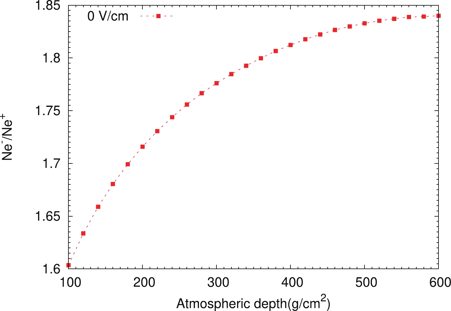
Figure 8. (color online) Ratio of electrons to positrons as a function of the atmospheric depth.
-
From the evaluations of Dwyer and Symbalisty et al., the threshold field strength for the development of the RREA process is about 1650 V/cm at LHAASO (4400 m a.s.l.). In order to get clues to the mechanism of electron acceleration in the thunderclouds, two typical strengths of thunderstorm electric field are selected, namely the field strength 1000 V cm-1 (smaller than the threshold strength for RREA) and the field strength 1700 V cm-1 (greater than the threshold strength for RREA).
Fig. 9 gives the number distributions of positrons in positive fields (the results in 0 V/cm are plotted just for comparison). The increase appears in positive electric fields, especially in the low energy band. With energy lower than 60 MeV, the number of positrons increases obviously. And the enhancement in +1700 V/cm (about 153%) is greater than that in +1000 V/cm (about 17%). As the energy increases, the influence of the electric field on particles gradually decreases. That is, the energy spectrum will become soft.
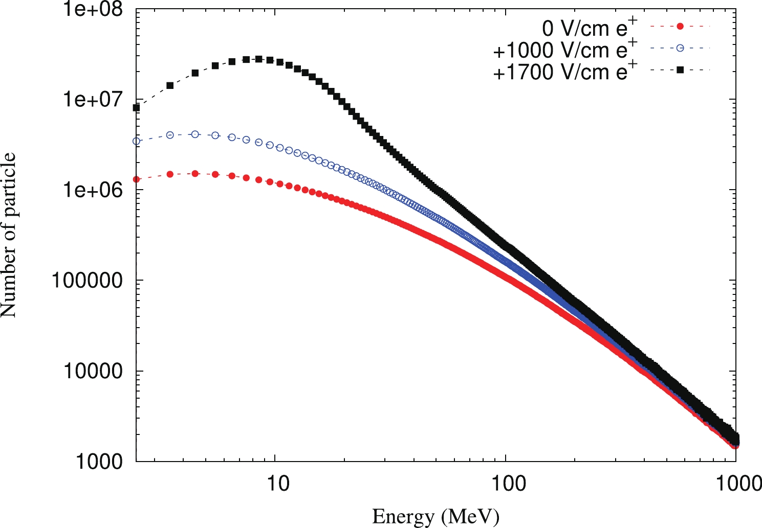
Figure 9. (color online) The number of positrons as a function of energy in positive fields.
Fig. 10 describes the variations of electron number with different energies in negative fields (the results in 0 V/cm are plotted just for comparison). When the electric field strength is 1700V/cm, the electron number exhibits an exponential increase at the low energy region. With energy less than 60 MeV, the increase is up to 14,310%. This is consistet with the RREA theory. From this figure, we can see that when the energy is lower than a few tens of MeV, the increase of electrons in
$ –1000 $ V/cm (about 42%) is far less than the increase in$ –1700 $ V/cm. Based on the results of the above two figures, we also can conclude that the negative electric field has a more obvious effect on particles than positive fields. The acceleration processes in two typical strengths of fields were discussed in detail in Ref. [90].
Figure 10. (color online) The number of electrons and as a function of energy in negative fields.
-
Monte Carlo simulations are performed to study the electric field effects on the secondary positrons and electrons at LHAASO. The intensity and energy of the particles change significantly, and the variation amplitudes are closely related to the strength and polarity of the electric field. These results can explain some of the existing experimental phenomena involving the intensity increases and decreases. Now, LHAASO experimental facilities have been fully built and been operational and acquired data normally. The experimental data of KM2A and WCDA will be analyzed, and the correlations between the variations of cosmic rays and thunderstorm electric fields will be studied. With the simulation and experimental results, we can better understand the data changes in LHAASO experiments during thunderstorms. At the same time, these results may provide important information for studying the acceleration mechanism of secondary charged particles by electric fields and the possible physical mechanism of lightning triggered by high energy cosmic rays.
Chapter 7 Solar and Heliospheric Physics and Interdisciplinary Research with LHAASO
- Received Date: 2021-12-02
- Available Online: 2022-03-15
Abstract: In the following sub-sections, studies of solar-heliospheric effects on cosmic rays, investigating a possible link between cosmic ray flux and Earth’s climate, and detection of MeV-range γ-rays from thunderstorms with the data from LHAASO will be discussed; geophysical research with environmental neutrons will be introduced, and some Monte Carlo simulation results about effects of thunderstorm electric fields on LHAASO observations of cosmic rays will be given.


 DownLoad: