


 Abstract
 HTML
HTML Reference
 Related
 PDF
PDF


-
A Little Bang can be produced by ultra-relativistic heavy-ion collisions, which provides a venue to learn about properties of deconfined quark matter, the strong interaction as well as antimatter nuclei [1-6]. Many probes which correspond to different evolution stages of heavy-ion collisions have been used to pin down the behavior of quark matter and hadronic matter at Relativistic Heavy Ion Collider (RHIC) and the Large Hadron Collider (LHC), see e.g. Refs. [7-12]. Besides collisions of very heavy ions, e.g. Au + Au or Pb + Pb, RHIC or LHC also have plans to collide lighter ions, e.g. the
$ ^{16} {\rm{O}}$ +$ ^{16} {\rm{O}}$ system. In such light nuclei, especially for 4N nuclei, an α-clustered structure is very likely. Actually, the α-clustered structure of stable nuclei has been one of the most interesting topics in nuclear physics community [13-21] since the α-cluster model was first proposed by Gamow. Broniowski et al. proposed that this kind of nuclear structure phenomenon can be demonstrated in relativistic heavy-ion collisions [22] and much progress has been achieved in recent years [23-28].The forward–backward (FB) correlation between final-state charged particle elliptic anisotropies [29, 30] or multiplicities in two separated η windows is a useful observable in high-energy hadron or nuclear collisions to study the dynamics of particle production mechanism [31-34]. Forward–backward rapidity correlation has been discussed in different frameworks such as two-step models [35], PYTHIA with color reconnection [36], the dual parton model [37] and the color glass condensate model [38, 39], and it is taken as a good tool to verify various models. Previous researches on asymmetrical collision systems can be found in literature [40-43]. Experimental studies on long-range correlations (LRC) at the LHC can be found in Refs. [44, 45]. The relationships between FB multiplicity correlation with centrality [46-48], negative binomial distribution (NBD) [49-53] and momentum [54, 55] have been discussed in different literature. Other related observations, such as multiplicity asymmetry variable C and its variance [56, 57] and two-particle correlation function
$ C(\eta _{1},\eta _{2}) $ [58-62] are also discussed. The origin of forward–backward multiplicity correlations is investigated in Refs. [31, 32].The study of correlations among particles produced in different pseudo-rapidity (η) regions may deepen our understanding of particle production mechanisms. In the framework of the dual parton model of nucleus–nucleus collisions, the FB correlations were considered to be the sum of long- and short-range correlations. LRC extends over a wider range of η difference, and originates from fluctuations associated with the particle-emitting sources. Short-range correlations (SRC), which quickly diminish as the pseudo-rapidity distance increases, come mainly from sources such as resonance decay and jets [63].
In high-energy nucleon–nucleon collisions (
$ \sqrt{s}\gg $ 100 GeV), the non-singly diffractive inelastic cross section increases significantly with energy, as does the magnitude of the long-range forward–backward multiplicity correlations [64]. When raising the center of mass energy$ \sqrt{s_{NN}} $ from 200 to 6370 GeV, FB correlations might allow us to decouple long-range correlations from short-range correlations and provide the information of collided light nuclei, if it is built up with exotic nuclear structures such as α-clusters. In a previous work, we use a forward–backward correlation factor$C(N_{\rm f},N_{\rm b})$ to investigate the correlation feature and found its sensitivity to initial nuclear structure [65]. Here we use Pearson's correlation coefficient to check our conclusion and make it more solid for such a probe. In fact, it is found that a system scan experiment could provide a good way to distinguish the exotic α-clustered nuclear structure from the Woods–Saxon structure.The rest of the paper is arranged as follows: In Section II a brief introduction to the AMPT model is presented. Section III presents the centrality and system dependences of the FB multiplicity correlation. Section IV describes how to distinguish the structure of light nuclei through FB multiplicity correlation, and then a summary is given in the end.
-
A Multi-Phase Transport (AMPT) model as a hybrid dynamic model is employed to calculate different collision systems. The AMPT model succeeds in describing extensive physics topics for relativistic heavy-ion collisions at RHIC and LHC energies, e.g., the
$ p_{T} $ distribution of charged particles [66], hadron Hanbury Brown and Twiss correlation [67], dihadron azimuthal correlation [68], collective flows [69, 70], as well as chiral magnetic effects and so on [71]. AMPT consists of four main components: (a) the initial conditions including the spatial and momentum distributions of mini-jet partons and soft string excitations, which are obtained from the HIJING model; (b) partonic cascade [72], whereby interactions among partons are described by equations of motion for their Wigner distribution functions; (c) hadronization, which is conversion from the partonic to the hadronic matter; and (d) hadronic interactions, based on the ART (A Relativistic Transport) model [73], including baryon–baryon, baryon–meson, and meson–meson elastic and inelastic scatterings. There are two versions of AMPT: (1) the AMPT version with a string melting mechanism, in which a partonic phase is generated from excited strings in the HIJING model, where a simple quark coalescence model is used to combine the partons into hadrons, and (2) the default AMPT version which only undergoes a pure hadron gas phase. Details of the AMPT model can be found in reviews [74, 75].We use the string-melting version of AMPT in this article. The initial nucleon distribution inside a nucleus is configured in the HIJING model [76] with the pattern of the Woods–Saxon distribution and the exotic nucleon distribution is embedded to study the α-clustered structure of
$ ^{16} {\rm{O}}$ . For details, parameters of the tetrahedral structure of$ ^{16}\mathrm{O} $ are inherited from an extended quantum molecular dynamics (EQMD) model [16], which is extended from the quantum molecular dynamics (QMD) model. With the effective Pauli potential, the EQMD model can give the reasonable α-cluster configurations for nuclei with 4N and even 4N + valence nucleons. For the four αs in the tetrahedral structure, we put them at the vertices with side length of 3.42 fm so that it gives a similar rms-radius (2.699 fm) to the Woods–Saxon (WS) configuration (2.726 fm) as well as the experimental data (2.6991 fm) [77], while nucleons inside each α are initialized using the Woods–Saxon distribution introduced in the HIJING model. -
Forward–backward multiplicity correlation can be expressed as Pearson's correlation coefficient of forward multiplicity
$ N_{\rm f} $ and backward multiplicity$ N_{\rm b} $ ,$ b_{\rm corr} = \frac{\left \langle N_{\rm b}N_{\rm f} \right \rangle-\left \langle N_{\rm b} \right \rangle\left \langle N_{\rm f} \right \rangle}{\sqrt{\left \langle N_{\rm b}^{2} \right \rangle-\left \langle N_{\rm b} \right \rangle^{2}}{\sqrt{\left \langle N_{\rm f}^{2} \right \rangle-\left \langle N_{\rm f} \right \rangle^{2}}}} = \frac{D_{\rm bf}^2}{D_{\rm bb} D_{\rm ff}}, $

(1) where
$ N_{\rm f} $ and$ N_{\rm b} $ are the numbers of charged particles falling into the forward and backward pseudorapidity intervals$ \delta \eta $ respectively and$ D_{\rm bf} $ ,$ D_{\rm bb} $ , and$ D_{\rm ff} $ represent the backward–forward, backward–backward, and forward–forward dispersions. This definition has been applied in some data analyses and model simulations [34, 46-48, 78]. In the present study, we follow this equation to investigate the system and centrality dependence, especially for the study of α-clustering nuclei.Here two intervals separated symmetrically around
$ \eta = 0 $ with variable width$ \delta \eta $ ranging from 0.2 to 0.8 are defined as “forward” ($ \eta >0 $ ) and “backward” ($ \eta <0 $ ). Correlations between multiplicities of charged particles are studied as a function of the gap between the windows$ \eta _\text{gap} $ , namely the distance between lower and upper boundary of forward and backward η windows.Reference multiplicities are used here to reduce the influence of centrality selection on forward–backward multiplicity correlations. The parameters are set as (a)
$ \delta \eta = 0.2 $ , and$ \eta _\text{gap} $ = 0, 0.2, 0.4, 0.6, 0.8, 1.0, 1.2, 1.4 and 1.6. For$ \eta _\text{gap} $ = 0, 0.2 and 0.4, reference multiplicity is set in$ 0.5<\left | \eta \right |<1.0 $ . For$ \eta _\text{gap} $ = 0.6 and 0.8, the reference multiplicity is the sum of multiplicities in$ \left | \eta \right |<0.3 $ and$ 0.8<\left | \eta \right |<1.0 $ . For$ \eta _\text{gap} $ = 1.0, 1.2, 1.4 and 1.6, reference multiplicity is obtained from$ \left | \eta \right |<0.5 $ . A similar approach can be found in [34, 47, 48]; (b)$ \delta \eta = 0.4 $ , and$ \eta _\text{gap} $ = 0, 0.2, 0.4, 0.6, 0.8, 1.0 and 1.2. For$ \eta _\text{gap} $ = 0, 0.2 and 0.4, reference multiplicity is set in$ 0.7<\left | \eta \right |<1.2 $ . For$ \eta _\text{gap} $ = 0.6 and 0.8, the reference multiplicity is the sum of multiplicities in$ \left | \eta \right |<0.3 $ and$ 1.0<\left | \eta \right |<1.2 $ . For$ \eta _\text{gap} $ = 1.0 and 1.2, reference multiplicity is obtained from$ \left | \eta \right |<0.5 $ ; (c)$ \delta \eta = 0.6 $ , and$ \eta _\text{gap} $ = 0, 0.2, 0.4, 0.6, and 0.8. For$ \eta _\text{gap} $ = 0, 0.2 and 0.4, reference multiplicity is set in$ 0.9<\left | \eta \right |<1.4 $ . For$ \eta _\text{gap} $ = 0.6 and 0.8, the reference multiplicity is the sum of multiplicities in$ \left | \eta \right |<0.3 $ and$ 1.2<\left | \eta \right |<1.4 $ ; (d)$ \delta \eta = 0.8 $ , and$ \eta _\text{gap} $ = 0, 0.2 and 0.4. The reference multiplicity is set in$ 1.1<\left | \eta \right |<1.6 $ . -
Generally speaking, collisions at higher energies give increasing values of mean multiplicity, leading to relatively larger correlation strengths
$ b_\text{corr} $ [78]. In order to obtain the relationship between correlation coefficient$ b_\text{corr} $ and$ \eta _\text{gap} $ , it is natural to check the pseudorapidity distribution first. We present the AMPT results of the$ {\rm d}N_{\text{ch}}/{\rm d}\eta $ with the experimental results for a range of collision centralities. The centrality of collisions is characterized by the number of final-state charged particles ($ N_{\rm ch} $ ). Figure 1 shows the pseudorapidity distributions of the charged particles including$ \pi ^{\pm } $ ,$ K^{\pm } $ , p and$ \bar{p} $ in Au + Au minibias collisions (impact parameter$ b = 0 -13.96 $ fm) at$ \sqrt{s_{NN}} $ = 200 GeV for different centrality bins for$ -5.4< $ $ \eta <5.4 $ . To compare with the experimental results, we do not give the transverse momentum cut here. We can see that the first two centrality bins (namely 0%–6%, 6%–15%) are a bit lower and the last three centrality bins (namely 25%–35%, 35%–45%, and 45%–55%) are a bit higher than those of Au + Au collision experimental data [79]. The difference in pseudorapidity distribution will, to some extent, explain the following calculation results we obtain.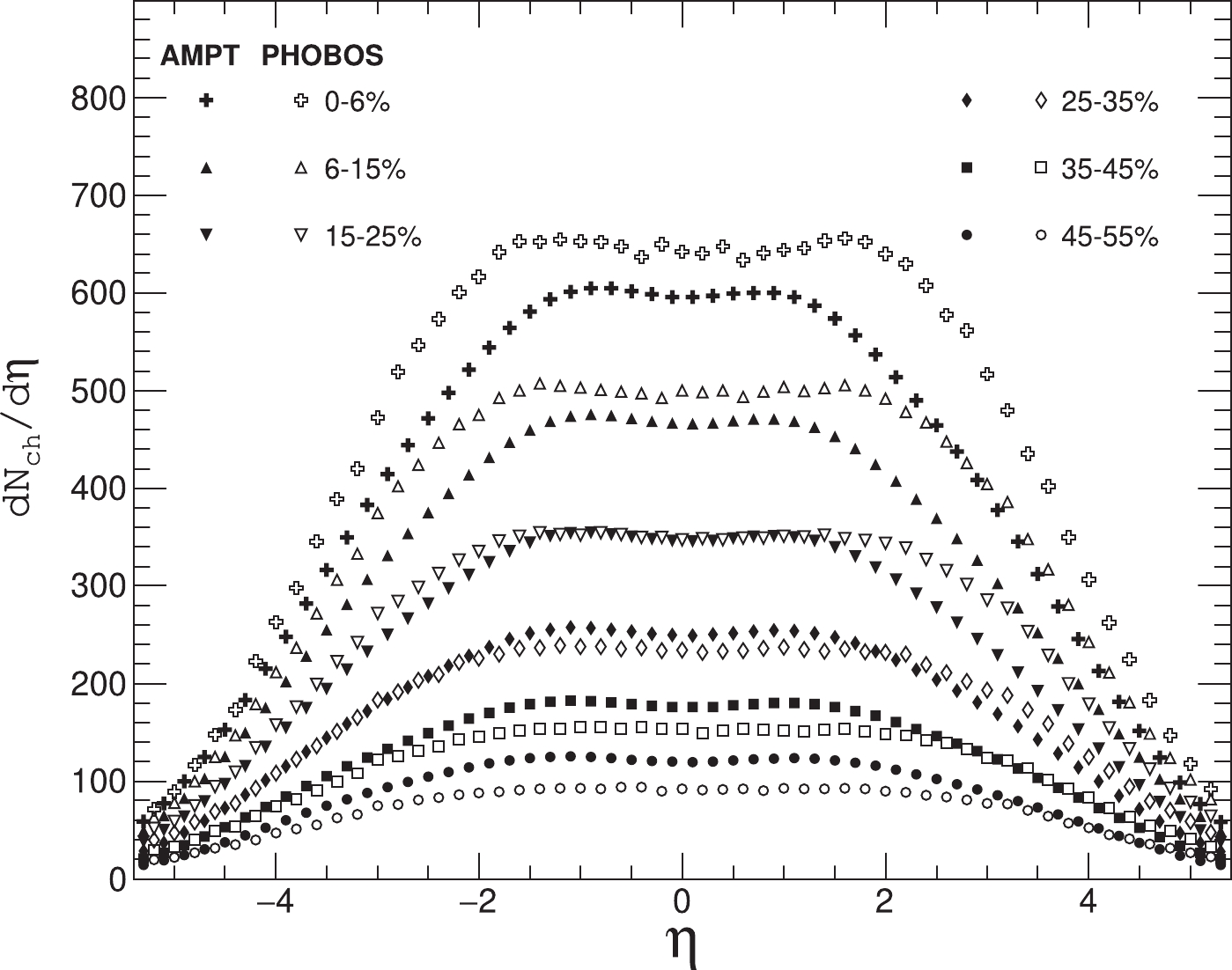
Figure 1. AMPT results of pseudorapidity distribution
${\rm d}N_{\rm ch}/{\rm d}\eta$ for charged particles including$\pi ^{\pm }$ ,$K^{\pm }$ , p and$\bar{p}$ , of Au + Au collisions (impact parameter$b = 0 -13.96$ fm) at$\sqrt{s_{NN}}$ = 200 GeV.Figure 2 shows the distributions of the Au + Au minibias collision events on the
$ N_{\rm b}-N_{\rm f} $ plane at$ \sqrt{s_{NN}} $ = 200 GeV for centrality bins of 0%–10%, 10%–20%, 20%–30%, 30%–40%, 40%–50% and 50%–60%. We select the charged hadrons with transverse momentum cut ($ 0.2<p_{\rm T}<3 $ ) GeV/c, pseudorapidity cut$ 0.8<\eta <1 $ for the forward window and$ -1<\eta <-0.8 $ for the backward window. The dashed lines guide eyes for the equal values of$ N_{\rm b} $ and$ N_{\rm f} $ .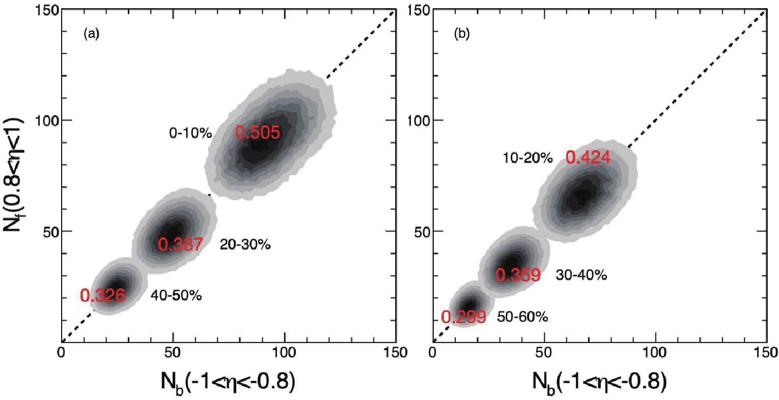
Figure 2. (color online) Distributions of Au + Au minibias collision events on the
$N_{\rm b}-N_{\rm f}$ plane at$\sqrt{s_{NN}}$ = 200 GeV for different centrality bins. Red text inside the contours show the value of “eccentricity”$\varepsilon_2$ of the corresponding 2-dimensional$N_{\rm b}-N_{\rm f}$ plots. -
Figure 3 shows the FB multiplicity correlation coefficient
$ b_\text{corr} $ as a function of$ \eta _\text{gap} $ and for different widths of the η windows ($ \delta \eta $ ) in Au + Au collisions with different centralities at$ \sqrt{s_{NN}} $ = 200 GeV. It is observed that the magnitude of FB correlation strength drops with the increase of centrality, i.e. from central to peripheral collisions, which is consistent with the previous experimental observation in Ref. [34].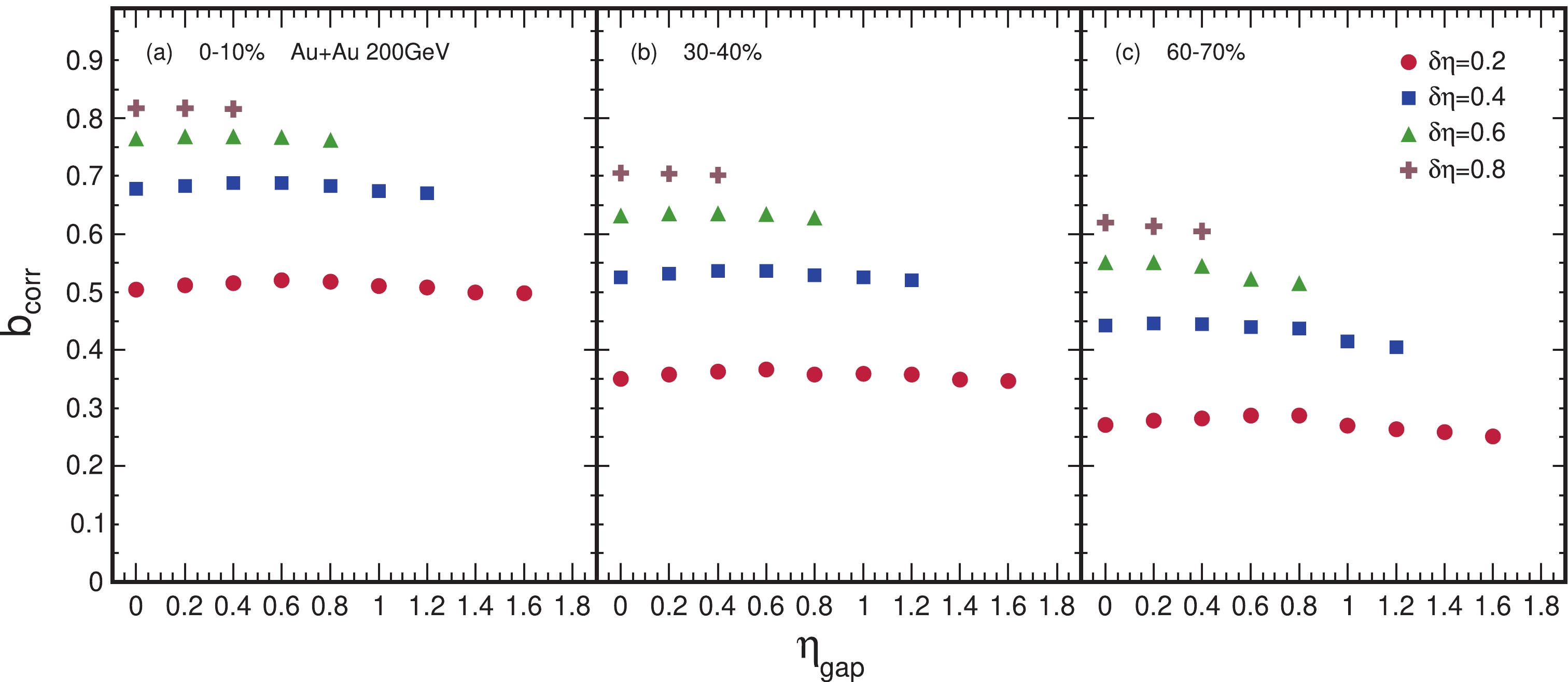
Figure 3. (color online) FB multiplicity correlation coefficient
$ b_\text{corr} $ through AMPT model as a function of$ \eta _\text{gap} $ and for different widths of the η windows ($ \delta \eta $ ) in$ ^{197} {\rm{Au}}$ +$ ^{197} {\rm{Au}}$ collisions at$ \sqrt{s_{NN}} $ = 200 GeV for centralities of (a) 0%-10%, (b) 30%-40%, and (c) 60%-70%.Providing that there is a two-dimensional Gaussian distribution in the
$ N_{\rm b}-N_{\rm f} $ plane with standard deviation$ \sigma _{x} = \sigma _{y} $ , which corresponds to the situation that the centrality bin width goes to zero, this simplified assumption gives$ b_\text{corr} = 0 $ . When the centrality bin width is larger, the situation can be simply understood as putting multiple Gaussian distributions one after another with gradually decreasing σ along the axis of$ N_{\rm b} = N_{\rm f} $ , giving a gradually increasing$ b_\text{corr} $ . If we look back at the charged-particle multiplicity distribution in Ref. [80], where in each centrality bin there are the same number of events, but the wider the$ N_{\rm ch} $ distribution the higher the centrality bin (more central collision). That is to say, there is a longer projection on the axis of$ N_{\rm b} = N_{\rm f} $ , which gives relatively bigger$ b_\text{corr} $ . Related discussion can be found in Ref. [48] by roughly treating the distributions in$ N_{\rm b}-N_{\rm f} $ as a two-dimensional Gaussian.For those distributions of events where different centrality bins in the
$ N_{\rm b}-N_{\rm f} $ plane are similar in shape, we can also use the “eccentricity”$ \varepsilon_2 $ to describe the$ N_{\rm b}-N_{\rm f} $ event distribution, where$ \varepsilon _{2}{\rm e}^{{\rm i}2\Phi_{2}} = -\left \langle n^{2}{\rm e}^{{\rm i}2\phi_{\rm bf}} \right \rangle/\left \langle n^{2} \right \rangle $ . Here$ n = \sqrt{N_{\rm b}'^2+N_{\rm f}'^2} $ and$ \phi_{\rm bf} = \tan^{-1}\left({N_{\rm f}'}/{N_{\rm b}'}\right) $ , where$ (N_{\rm b}', N_{\rm f}') = $ $ (N_{\rm b} -\bar{N}_{\rm b}, N_{\rm f} -\bar{N}_{\rm f}) $ for each event, and$ (\bar{N}_{\rm b},\bar{N}_{\rm f}) $ is the mean value of$ (N_{\rm b}, N_{\rm f}) $ . Note that the “eccentricity” is not the initial anisotropy in the transverse coordinate plane which is often used in heavy-ion collisions. We just use this definition to describe the event distribution in the$ N_{\rm b}-N_{\rm f} $ plane. When “eccentricity”$ \varepsilon_2 $ tends to 0, the spread of events on the$ N_{\rm b}-N_{\rm f} $ plane is close to circular, and in the language of correlation coefficient$ b_\text{corr} $ ,$ N_{\rm b} $ and$ N_{\rm f} $ are not related. On the contrary, a large$ \varepsilon_2 $ represents strong positive linear correlation between$ N_{\rm f} $ and$ N_{\rm b} $ . Correlation coefficient$ b_\text{corr} $ or “eccentricity”$ \varepsilon_2 $ , or the$ e\equiv \sqrt{1-\sigma _{b}^{2}/\sigma _{a}^{2}} $ used in Ref. [48] are equivalent as long as we are talking about symmetric systems, where events on the$ N_{\rm b}-N_{\rm f} $ plane are distributed diagonally. The corresponding “eccentricity” coefficient$ \varepsilon_2 $ is also marked in Fig. 2 and it is obvious from the figure, from central to peripheral collisions, the shadow region gradually changes from a slender ellipse to a circle and the corresponding “eccentricity” coefficient$ \varepsilon_2 $ decreases continuously.Ref. [47] shows a related calculation for Pb + Pb collisions at
$ \sqrt{s_{NN}} $ = 2.76 TeV. The discussion above can easily explain its problem that$ b_\text{corr} $ does not follow any regular pattern in terms of centrality selection.Quantitative differences with the experimental results can partly be explained through the difference in
$ N_{\rm ch} $ distribution (Fig. 1) mentioned above. For the centrality bin 0%-10%, the AMPT gives a value of$ b_\text{corr} $ approximately equal to 0.5, which is smaller than the results$ 0.5< $ $ b_\text{corr}<0.6 $ obtained in the experiment. This is expected because in that centrality range the AMPT gives a relatively lower$ {\rm d}N_{\text{\rm ch}}/{\rm d}\eta $ than that of RHIC experiments, therefore the event distribution on the$ N_{\rm b}-N_{\rm f} $ plane along the diagonal should also be shorter than in the RHIC experiments. Similarly, for the centrality bin 30%–40% and 60%–70%, we give values of$ b_\text{corr} $ approximately equal to 0.35 and 0.3, which are larger than the experimental results 0.2 and 0.1, respectively. It can also be explained by the AMPT model giving a relatively higher$ {\rm d}N_{\text{\rm ch}}/{\rm d}\eta $ . However, we do not see the sharply decreasing behavior with$ \eta _\text{gap} $ for the 60%-70% centrality bin.Figure 4 shows the FB multiplicity correlation coefficient
$ b_\text{corr} $ as a function of$ \eta _\text{gap} $ and for different widths of the η windows in pp collisions at three collision energies$ \sqrt{s_{NN}} $ = 10, 200, and 5020 GeV. At each collision energy,$ b_\text{corr} $ is found to decrease slowly with the increase of$ \eta _\text{gap} $ . Our calculations are in good agreement with those of Ref. [78] in quantity: Fig. 4(b) shows that the result of 200 GeV is slightly smaller than that of 0.9 TeV, and Fig. 4(c) displays that the value$ b_\text{corr} $ of 5020 GeV is between that of 2.76 TeV and 7 TeV. It is found that the pedestal value of$ b_\text{corr} $ increases with the collision energy, while the slope of the$ b_\text{corr} $ stays approximately constant, which indicates that the short-range correlation is similar at three energies, while the long-range correlation has stronger energy dependence.
Figure 4. (color online) Forward–backward correlation strength
$ b_\text{corr} $ as a function of$ \eta _\text{gap} $ and for different window widths$ \delta \eta $ = 0.2, 0.4, 0.6, and 0.8 in pp collisions at$ \sqrt{s_{NN}} $ = 10 (a), 200 (b), and 5020 (c) GeV. Note that the values of the data points in panel (a) are multiplied by 5.This analysis is extended to correlations between separated regions in the
$ \eta -\phi $ plane. Here ϕ is the azimuthal angle of momenta. The ϕ angle space is split into eight sectors with width$ \delta \phi = \pi /4 $ . This selection is motivated by a compromise between granularity and statistical uncertainty. The variable$ \phi_\text{sep} $ is the relative separation in azimuthal angle between centres of the forward sector and backward sector.The 2-dimensional distribution of
$ b_\text{corr} $ in$ p+p $ collision as a function of$ \eta_\text{gap} $ and$ \phi_\text{sep} $ is shown in Fig. 5 at$ \sqrt{s_{NN}} $ = 10, 200, and 5020 GeV. In Fig. 5(a),$ b_\text{corr} $ in the$ \eta -\phi $ plane gives an almost zero value. People may think forward–backward multiplicity is irrelevant in pp collisions at$ \sqrt{s_{NN}} $ = 10 GeV. However, this is not the case. At such a low energy, p+p collisions give almost zero number of charged particles in each forward and backward window, thus it is meaningless to talk about$ b_\text{corr} $ in this case. We can find a peak at the point ($ \eta _\text{gap} $ ,$ \phi_\text{sep} $ ) = (0, π) in Fig. 5(b). This could be the contribution of the final-state particles produced by back-to-back scattering. In Fig. 5(c), we find a ridge at$ \phi_\text{sep} $ = 0 and the value of$ b_\text{corr} $ decreases as the$ \eta _\text{gap} $ increases, which is consistent with the results from the ALICE Collaboration [78]. The azimuthal distribution of particles shows two peaks, centred at zero and at π, which indicates the jet structure. We can see clearly there are two contributions to the correlation coefficient$ b_\text{corr} $ : the SR contribution is concentrated within a rather limited region in the$ \eta -\phi $ plane within one unit of pseudorapidity, while the LR contribution manifests itself as a common pedestal in the whole region of observation. With the increase of collision energy, the number of strings (LR related) increases, which leads to the uplift of the pedestal and the amount of decay (SR related) increases, which leads to the formation of a peak at ($ \eta _\text{gap} $ ,$ \phi _\text{sep} $ ) = (0, 0).
Figure 5. (color online) 2D representation of
$ b_\text{corr} $ in pp collisions at (a)$ \sqrt{s_{NN}} $ = 10 GeV, (b)$ \sqrt{s_{NN}} $ = 200 GeV and (c)$ \sqrt{s_{NN}} $ = 5020 GeV for separated$ \eta -\phi $ window pairs with$ \delta \eta = 0.2 $ and$ \delta \phi = \pi /4 $ .$ \phi_\text{sep} $ is the relative separation (number of$ \delta \phi = \pi /4 $ ) in azimuthal angle between centres of the forward sector and backward sector.Figure 6 shows the 2-dimensional distribution of
$ b_\text{corr} $ in the symmetric collision systems from large to small systems, i.e. from$ ^{197} {\rm{Au}}$ +$ ^{197} {\rm{Au}}$ to$ ^{16} {\rm{O}}$ +$ ^{16} {\rm{O}}$ and$ ^{12} {\rm{C}}$ +$ ^{12} {\rm{C}}$ collisions, as a function of$ \eta _\text{gap} $ and$ \phi _\text{sep} $ at$ \sqrt{s_{NN}} $ = 200 GeV. Two ridges at$ \phi _\text{sep} $ = 0 and$ \phi _\text{sep} $ = π in Au + Au are observed for the most central collisions. In Au + Au peripheral collisions,$ b_\text{corr} $ in the$ \eta -\phi $ plane behaves similar to the$ p+p $ collision in Fig. 5(b) and the most central collision in O + O or C + C systems. In addition, the difference between light nuclei with different initial structures is negligible (for the reason given in the following text), so for brevity we do not show the comparison here. The two-ridge structure might relate to the elliptic flow. As we know the 30%–40% centrality events give the biggest$ v_{2} $ value, and the biggest relative$ b_\text{corr} $ difference between the ridge and valley emerges at the same centrality. Taking a typical elliptic flow event into consideration, there is a greater chance to see final-state particles when rotating$ \phi = 0 $ or$ \phi = \pi $ from the long axis and relatively small probability to see those when rotating$ \phi = {\pi }/{2} $ or$ \phi = {3\pi }/{2} $ , which explains the two ridges seen at$ \phi _\text{sep} $ = 0 and π and the two valleys seen at$ \phi = {\pi }/{2} $ and$ {3\pi }/{2} $ . It is the largest mean multiplicity, or to be more precise it is the longest projection along the axis$ N_{\rm b} = N_{\rm f} $ , that gives the relatively highest pedestal value in Fig. 6(a).
Figure 6. (color online) 2D representation of
$ b_\text{corr} $ at$ \sqrt{s_{NN}} $ = 200 GeV in$ ^{197} {\rm{Au}}$ +$ ^{197} {\rm{Au}}$ collision systems for (a) 0%-10%, (b) 30%-40%, and (c) 60%-70% centralities;$ ^{16} {\rm{O}}$ +$ ^{16} {\rm{O}}$ collision systems for (d) 0%-10%, (e) 30%-40%, and (f) 60%-70% centralities;$ ^{12} $ C +$ ^{12} $ C collision systems for (g) 0%-10%, (h) 30%-40%, and (i) 60%-70% centralities for separated$ \eta -\phi $ window pairs with$ \delta \eta = 0.2 $ and$ \delta \phi = \pi /4 $ . -
The calculated
$ b_\text{corr} $ of light nuclei with/without α-clustered structures for the minibias data and the data with impact parameter cut$ b<2.0 $ fm are shown in Fig. 7 as a function of$ \eta_\text{gap} $ for$ \delta \eta $ ranging from 0.2 to 0.8. In$ ^{12} {\rm{C}}$ +$ ^{12} {\rm{C}}$ and$ ^{16} {\rm{O}}$ +$ ^{16} {\rm{O}}$ collisions at$ \sqrt{s_{NN}} $ = 200 GeV, the FB correlation strengths fall sharply with the rapidity gap. This phenomenon is considered to be the result of short-range correlation. This can be easily understood as short-range correlations from clusters produced around$ \eta = 0 $ often push their charged decay products into both regions simultaneously. At$ \sqrt{s_{NN}} $ = 6370 GeV, the short-range component of$ b_\text{corr} $ is found to be weak, nearly overwhelmed by thermalization or interactions. If the effect of final-state SRCs can be ignored, we can study the source information, in this paper specifically for the different structures of light nuclei, more clearly through the$ b_\text{corr} $ .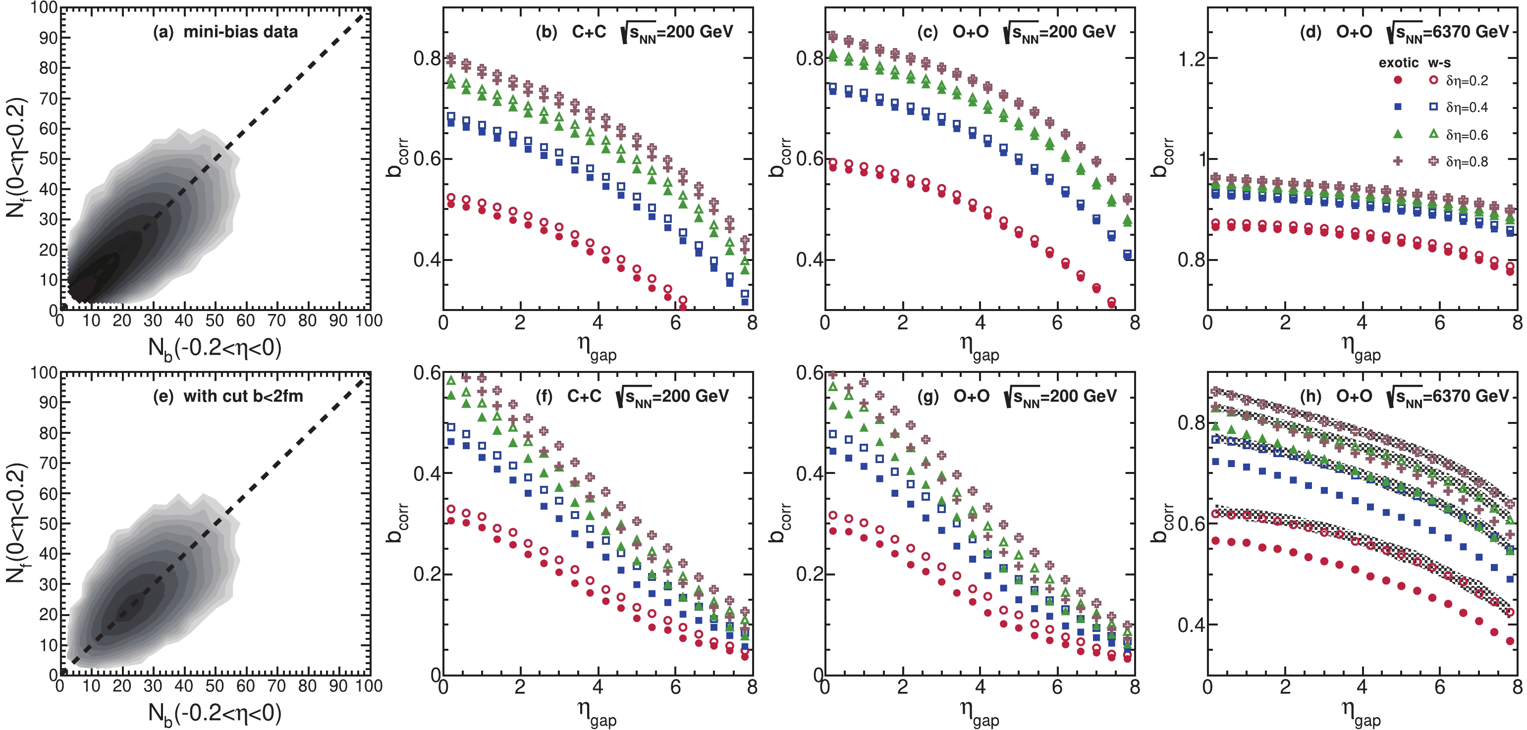
Figure 7. (color online) Upper panels: (a) the distribution of
$ ^{16} {\rm{O}}$ +$ ^{16} {\rm{O}}$ events on the$ N_{\rm b}-N_{\rm f} $ plane. FB multiplicity correlation coefficient$ b_\text{corr} $ as a function of$ \eta _\text{gap} $ and for different widths of the η windows in (b)$ ^{12} {\rm{C}}$ +$ ^{12} {\rm{C}}$ collisions with different α-clustered structures at$ \sqrt{s_{NN}} $ = 200 GeV; (c)$ ^{16} {\rm{O}}$ +$ ^{16} {\rm{O}}$ collisions at$ \sqrt{s_{NN}} $ = 200 GeV; (d)$ ^{16} {\rm{O}}$ +$ ^{16} {\rm{O}}$ collisions at$ \sqrt{s_{NN}} $ = 6370 GeV. Lower panels: same as the upper panels except with the cut$ b<2 $ fm.Figure 7 (a) and (e) show the event distribution of
$ ^{16} {\rm{O}}$ +$ ^{16} {\rm{O}}$ collisions on the$ N_{\rm b}-N_{\rm f} $ plane at$ \sqrt{s_{NN}} $ = 6370 GeV with and without the cut$ b<2.0 $ fm, respectively. It is found that the minibias data have an accumulation at low multiplicity, which enhances the$ b_\text{corr} $ greatly and creates difficulties in distinguishing the different structures. To prevent the large number of low-multiplicity events from overwhelming the features of high-multiplicity ones, the cut in impact parameter$ b<2 $ fm is used. It is found from Fig. 7 (h) that the tetrahedral four α-clustered structure of$ ^{16} {\rm{O}}$ shows an obvious smaller$ b_{\rm corr} $ than that of the Woods-Saxon one, where the difference between the WS (open circle) and the tetrahedral (solid circle) structures is clearly visible. Furthermore, to make α-clustering structure stand out, we add two more collision simulations, namely the WS-configured$ ^{14} {\rm{N}}$ +$ ^{14} {\rm{N}}$ and$ ^{19} {\rm{F}}$ +$ ^{19} {\rm{F}}$ , which are close to$ ^{16} {\rm{O}}$ +$ ^{16} {\rm{O}}$ in mass number. Figure 7(h) shows the correlation results of$ ^{14} {\rm{N}}$ +$ ^{14} {\rm{N}}$ and$ ^{19} {\rm{F}}$ +$ ^{19} {\rm{F}}$ , where the gray region with upper edge for$ ^{14} {\rm{N}}$ +$ ^{14} {\rm{N}}$ and lower edge for$ ^{19} {\rm{F}}$ +$ ^{19} {\rm{F}}$ . We can see that the$ b_\text{corr} $ of$ ^{16} {\rm{O}}$ +$ ^{16} {\rm{O}}$ with the Woods-Saxon structure are almost identical to the results of the$ ^{14} {\rm{N}}$ +$ ^{14} {\rm{N}}$ and$ ^{19} {\rm{F}}$ +$ ^{19} {\rm{F}}$ . In other words, if we perform a system scan of$ b_\text{corr} $ for$ ^{14} {\rm{N}}$ +$ ^{14} {\rm{N}}$ ,$ ^{16} {\rm{O}}$ +$ ^{16} {\rm{O}}$ and$ ^{19} {\rm{F}}$ +$ ^{19} {\rm{F}}$ and observe significant smaller$ b_\text{corr} $ for$ ^{16} {\rm{O}}$ +$ ^{16} {\rm{O}}$ with respect to the other two systems, we could argue there is a tetrahedral structure of$ ^{16} {\rm{O}}$ .To further clarify the difference between α-clustered and Woods–Saxon
$ ^{16} {\rm{O}}$ +$ ^{16} {\rm{O}}$ systems, we plot the$ N_{\rm b} - N_{\rm f} $ event distribution for$ ^{14} {\rm{N}}$ +$ ^{14} {\rm{N}}$ (WS),$ ^{16} {\rm{O}}$ +$ ^{16} {\rm{O}}$ (WS),$ ^{16} {\rm{O}}$ +$ ^{16} {\rm{O}}$ (tetrahedron) and$ ^{19} {\rm{F}}$ +$ ^{19} {\rm{F}}$ (WS) in Fig. 8 and the corresponding “eccentricity”$ \varepsilon_2 $ is written inside each panel. It is found from Fig. 8(a) to Fig. 8(d) that for$ \delta \eta = 0.2 $ the “eccentricity”$ \varepsilon_2 $ values are 0.622, 0.614, 0.556, 0.604, and the$ ^{16} {\rm{O}}$ +$ ^{16} {\rm{O}}$ (tetrahedron)$ \varepsilon_2 $ is smaller than the$ ^{16} {\rm{O}}$ +$ ^{16} {\rm{O}}$ (WS) case. In Fig. 9 we project the$ N_{\rm b} - N_{\rm f} $ event distribution onto the axis of$ N_{\rm b} $ =$ N_{\rm f} $ as well as its orthogonal axis. The axis of$ N_{\rm b} $ =$ N_{\rm f} $ is the major axis and its orthogonal axis is the minor axis. As we can see from Fig. 9(a) to Fig. 9(h), the mean multiplicities are of course increasing from$ ^{14} {\rm{N}}$ +$ ^{14} {\rm{N}}$ to$ ^{19} {\rm{F}}$ +$ ^{19} {\rm{F}}$ systems. However, the distribution width of tetrahedron system is narrower than the WS system along the major axis. Since the distributions along the minor axis show no difference between different$ ^{16} {\rm{O}}$ configurations, this is mainly because a narrower distribution along the major axis leads to the smaller value of “eccentricity”$ \varepsilon_2 $ for tetrahedron-configured$ ^{16} {\rm{O}}$ +$ ^{16} {\rm{O}}$ , hence the smaller value of$ b_\text{corr} $ . In order to explain the differences seen above, we count the standard deviation of the difference between number of participants in projectile and target, namely$ \sigma(N_{\rm part}^{\rm P}-N_{\rm part}^{\rm T}) $ . For the tetrahedron system it is 1.697 and for Woods–Saxon it is 1.859. It seems the tetrahedron$ ^{16} {\rm{O}}$ +$ ^{16} {\rm{O}}$ collision gives a more uniform, symmetrical and thermalized fireball, and the expansion and evolution emits the final particles more evenly or isotropically (independently and randomly) in the longitudinal direction. If we choose an appropriate window size$ \delta \eta $ (probably the characteristic size of the jet during proton collision) such as 0.4 or 0.6, we might well capture the differences between different configurations.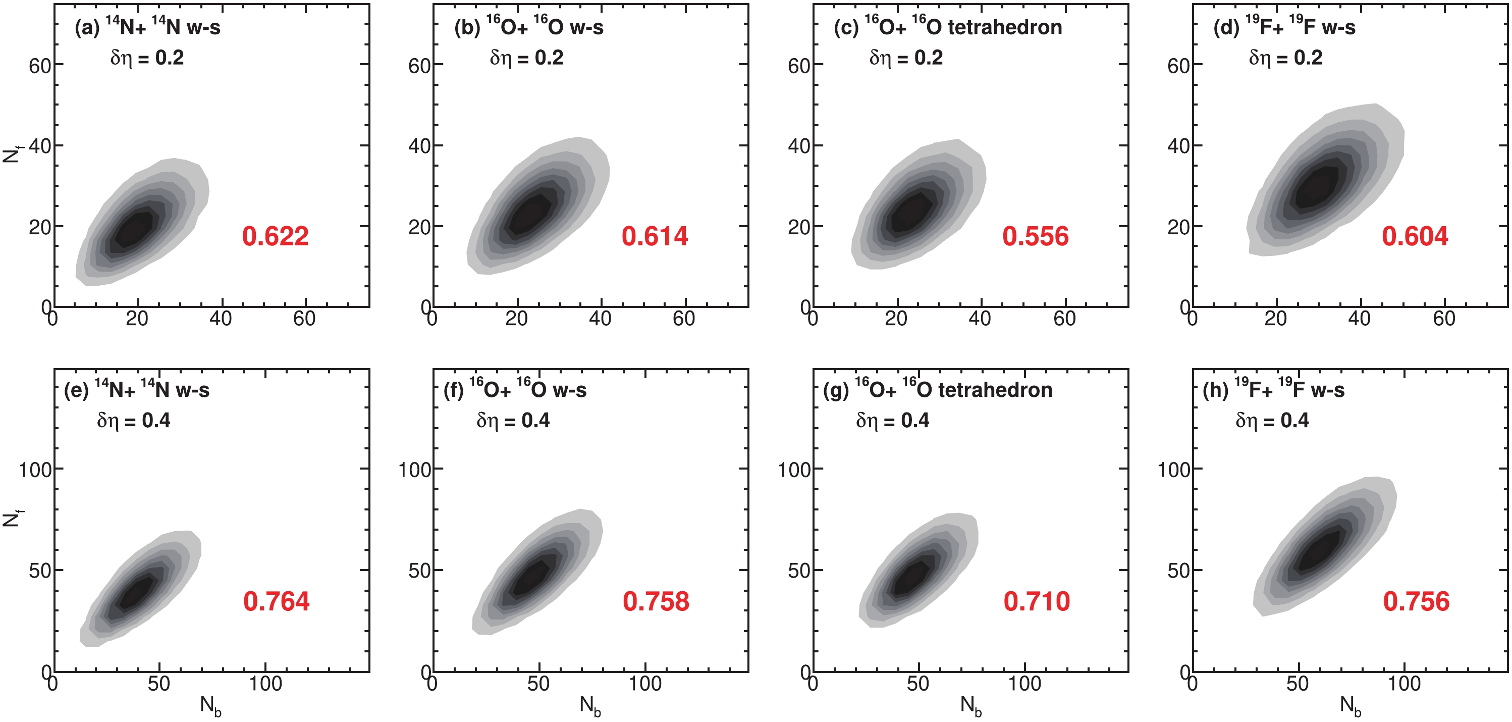
Figure 8. (color online) 2d
$ N_{\rm b} - N_{\rm f} $ plots for$ ^{14} {\rm{N}}$ +$ ^{14} {\rm{N}}$ (WS),$ ^{16} {\rm{O}}$ +$ ^{16} {\rm{O}}$ (WS),$ ^{16} {\rm{O}}$ +$ ^{16} {\rm{O}}$ (tetrahedron) and$ ^{19} {\rm{F}}$ +$ ^{19} {\rm{F}}$ (WS) (from left panel to right panel) at$ \sqrt{s_{NN}} $ = 6370 GeV with the corresponding “eccentricity” values marked in the respective plots.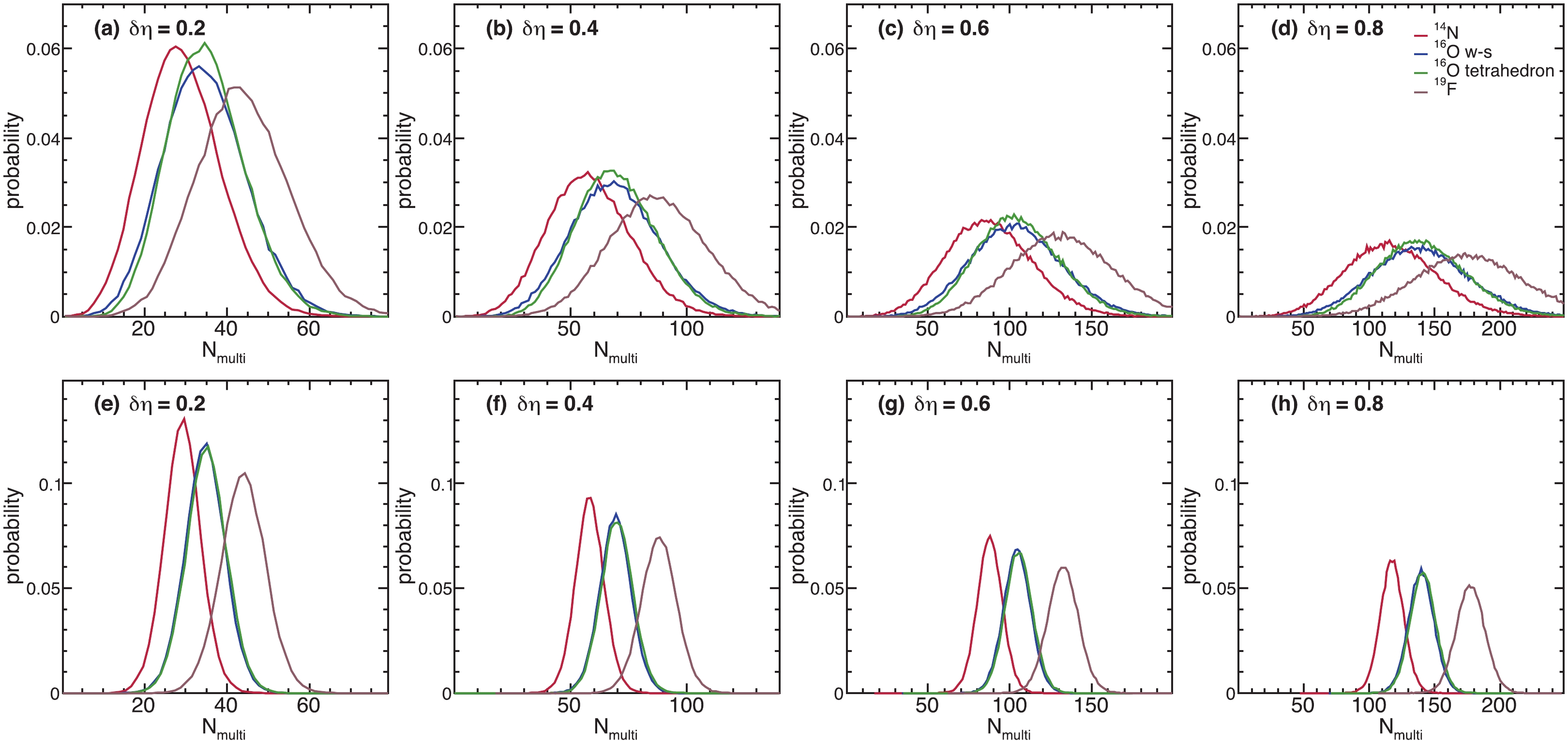
Figure 9. (color online) Projections of 2d
$ N_{\rm f} $ -$ N_{\rm b} $ distribution onto the axis of$ N_{\rm b} $ =$ N_{\rm f} $ (the first row) and its orthogonal axis (the second row) with different window widths$ \delta \eta $ for different collision systems at$ \sqrt{s_{NN}} $ = 6370 GeV. -
In summary, a systematic study on forward–backward multiplicity correlations
$ b_\text{corr} $ from large to small systems has been performed using the AMPT model. It is observed that the magnitude of FB correlation strength decreases from central to peripheral collisions for Au + Au at$ \sqrt{s_{NN}} $ = 200 GeV, which can be explained in a self-consistent way by taking the distribution of events as the superposition of a series of Gaussian distributions. An increasing FB correlation strength with the energy from$ \sqrt{s_{NN}} $ = 10 GeV, 200 GeV to 5.02 TeV is observed in$ p+p $ collision, which can be mainly attributed to the wider event distribution caused by the increase of mean multiplicity. In addition, it is found that correlations in the$ \eta -\phi $ plane can imply the shape of events.The correlations of particles created at early stages of the collisions can spread over large rapidity intervals, unlike the particles produced at later stages. Thus, the measurement of the long-range rapidity correlations of the produced particle multiplicities could give us some insight into the space-time dynamics of the early stages of collisions. Following this idea, we compare the
$ b_\text{corr} $ of α-clustered$ ^{16} {\rm{O}}$ +$ ^{16} {\rm{O}}$ with the results of WS-type system and find a visible difference between the two configurations. From the viewpoint of experimental measurements, we compare$ ^{16} {\rm{O}}$ +$ ^{16} {\rm{O}}$ results with$ ^{14} {\rm{N}}$ +$ ^{14} {\rm{N}}$ and$ ^{19} {\rm{F}}$ +$ ^{19} {\rm{F}}$ . It is found that the$ b_\text{corr} $ of the WS-configured$ ^{16} {\rm{O}}$ +$ ^{16} {\rm{O}}$ are almost identical to that of$ ^{14} {\rm{N}}$ +$ ^{14} {\rm{N}}$ and$ ^{19} {\rm{F}}$ +$ ^{19} {\rm{F}}$ , while the strength$ b_\text{corr} $ of α-clustered$ ^{16} {\rm{O}}$ +$ ^{16} {\rm{O}}$ are much smaller. The FB correlation strengths could be proposed as a probe to distinguish the exotic α-clustering pattern experimentally. We look forward to such experiments being carried out in future LHC experiments. Related experimental results will definitely provide a test and pose new challenges to these multiple-scattering models.
System scan of the multiplicity correlation between forward and backward rapidities in relativistic heavy-ion collisions using a multi-phase transport model
- Received Date: 2021-10-15
- Available Online: 2022-04-15
Abstract: A systematic study on forward–backward (FB) multiplicity correlations from large systems to small ones through a multi-phase transport model (AMPT) has been performed and the phenomenon that correlation strength increases with centrality can be explained by taking the distribution of events as the superposition of a series of Gaussian distributions. It is also found that correlations in the


 DownLoad: