Kotzinian-Mulders effect in semi-inclusive DIS within TMD factorization

The investigation of the internal structure of the nucleon remains a frontier of hadronic physics research. Azimuthal asymmetries in semi-inclusive deep inelastic scattering (SIDIS) are key observables to probe the spin dependent substructure of the nucleon. Measurements of azimuthal asymmetries are crucial to comprehending the transverse structure of the proton. The collinear picture utilized for DIS is not sufficiently appropriated to obtain various asymmetries in SIDIS, and the transverse momentum of the active quark in a nucleon must be added. The transverse momentum dependent (TMD) factorization [1, 2] approach can describe this asymmetry. The inclusive cross section of SIDIS can be expressed as a convolution of nonperturbative TMD parton distribution functions and fragmentation functions and perturbatively calculated partonic cross sections. In other words, the SIDIS cross section can be factorized into TMD parton distribution functions (PDFs) having the information of the active quark distributions with transverse momentum in the parent proton and the TMD parton fragmentation functions (FFs) illustrating the hadronizations of the struck quarks into the detected hadrons. The azimuthal asymmetries in SIDIS have been studied in many experiments. The early research published by the JLab, HERMES, CLAS, and COMPASS collaborations on azimuthal asymmetries in SIDIS production of charged hadrons are available in Refs. [3-23]. For both experimental and theorical reviews, refer to [24-28].

The various azimuthal asymmetries in SIDIS have been investigated theoretically in various studies (e.g. [29-31]). Generally, authors explore the SIDIS process at twist-two level in the parton model with TMDs and TMD FFs. Such processes can be described in terms of eight PDFs including six time reversal even and two time reversal odd PDFs. Among the leading-twist TMDs, the Kotzinian-Mulders (KM) function $g_{1T}(x,\vec{k}_T^2)$ [32] describing the probability of discovering a longitudinally polarized quark in a transversely polarized nucleon has rarely been considered to date. The $g_{1T}(x,\vec{k}_T^2)$ is chiral-even and can be reached in SIDIS combined with the unpolarized FF. In practice, $g_{1T}(x,\vec{k}_T^2)$ combined with the unpolarized FF $D_1$ can be accessed from double spin asymmetries (DSAs) $A_{LT}^{\cos(\phi_h-\phi_S)}$ in SIDIS. The reason is that both a longitudinally polarized beam and a transversely polarized target are necessary for the longitudinal polarization of the active quark. This DSA is usually referred to as the KM effect [32].

In Ref. [29], the authors studied the KM effect in SIDIS without scale evolution. In this study, we perform a more detailed phenomenological analysis of the KM effect in SIDIS within TMD factorization and compare them with the data from the COMPASS and HERMES collaboration [16, 23, 33]. Measurements have also been conducted for the KM effect in SIDIS with a neutron target [3, 34]. TMD factorization has been applied in many studies [35-40] focusing on various asymmetries in Drell-Yan and SIDIS processes. Beginning from the previous research by Collins-Soper-Sterman (CSS) [41, 42], the so-called TMD evolution following from factorization theorems has been fully developed in recent years. Similar phenomenological studies for asymmetries contributed by Sivers, Boer-Mulders, and Collins functions are discussed within TMD factorization in both Drell-Yan and SIDIS processes. The energy scale evolution is connected with the Sudakov form factor [42-44] after solving the evolution equation, which can be split into a perturbatively computable part $S_{\rm{pert}}$ and a nonperturbative part $S_{\rm{NP}}$. To be precise, TMD evolution is performed in the coordinate b-space related by momentum space via a Fourier transformation. The use of b-space simplifies the expressions of the cross sections from convolutions in the momentum space into simple products of b dependent TMDs. Subsequently, the Sudakov evolution kernel becomes non-perturbative at large separation distances b, whereas at small $b \ll 1/\Lambda_{\rm{QCD}}$, it can be perturbatively calculated order by order for a strong coupling constant $\alpha_s$. A two dimensional Fourier transform must be performed to the physical $k_\perp$ space for the corresponding TMDs to calculate the measured cross sections. For a b-space TMD at a initial scale μ, it can be expressed as a convolution of a perturbatively calculated C-coefficient and a collinear correlation function at the same scale μ. The collinear correlation function can be considered the collinear counterpart of the b-space TMD, and it can be obtained using perturbation theory. Specifically, the KM function $g_{1T}$ in the coordinate space can be expressed as a convolution of the corresponding C-coefficient and the collinear correlation function, $\tilde{g}(x)$. In this paper, the perturbative Sudakov form factors are considered up to the next-to-leading order (NLO) accuracy, and we adopt the tree-level results of the C-coefficients since the C-coefficients for $g_{1T}$ still remain in the leading order (LO). The nonperturbative Sudakov form factors in the unpolarized differential cross section were obtained from Ref. [45], which followed the CSS formalism with the $b^*$-prescription. We performed the TMD evolution to attain the fragmentation function and $\tilde{g}(x)$ at a initial scale $\mu_b = c/b^*$ using the evolution package QCDNUM [46]. Based on the above considerations, in this paper, we estimate the KM effect within the TMD factorization and compare the results with the HERMES and COMPASS measurements. In addition, we perform predictions for the KM effect within the TMD factorization at EIC and EicC kinematics.

The remainder of this paper is organized as follows. In Sec. II, we review the basic framework of TMD evolution for accessing the KM effect in the SIDIS process. In Sec. III, we present the numerical calculation of the KM effect for the underlying process at the kinematics of HERMES and COMPASS measurements, respectively. The paper is concluded in Sec. IV.

We mostly follow the framework of a recent paper [36], which studied the Sivers asymmetry of the Drell-Yan process within TMD factorization. We consider the SIDIS process in which a virtual photon $q_\mu = l_\mu-l_\mu'$ with invariant mass $Q^2 = -q^2$ is exchanged:

where a longitudinal polarized lepton scatters off a transverse polarized target nucleon with polarization S and momentum P. Inside the target, the photon hits the active quark with momentum k and then changes it to p. We use the usual SIDIS variables [47]:

When $P_{h\perp} \ll Q$, the TMD factorization can be applied, and the SIDIS differential cross section including $\cos(\phi_h-\phi_S)$ term can be expressed as [48]

where $\varepsilon = \dfrac{1-y-\frac{1}{4}\gamma^2 y^2}{1-y+\frac{1}{2}y^2+\frac{1}{4}\gamma^2 y^2}$ and

and $\vec{P}_{h\perp}$ is the transverse momentum of the final state hadron with respect to the lepton plane. Here, $F_{UU}$ is the spin-averaged structure function, and $F_{LT}$ is the spin dependent structure function contributing to the $\cos(\phi_h-\phi_S)$ azimuthal asymmetry. The unit vector $\hat{\vec{h}} = \vec{P}_{h\perp}/|\vec{P}_{h\perp}|$. We introduce $\phi_h$ and $\phi_S$ as the azimuthal angles of the transverse momentum vector of the final-state hadron and transverse spin of the target, respectively. Following the Trento conventions [49], these angles are defined in the target rest frame with the $\hat{z}$ axis along the virtual-photon momentum and the $\hat{x}$ axis along the lepton transverse momentum. In Eq. (3), the terms that we are not interested in have been ignored. We have also adopted the notation

where $\vec{k}_T$ and $\vec{p}_T$ are the corresponding transverse momentum componments of $k,p$, respectively. The second term on the r.h.s. of Eq. (3) refers to a leading twist effect involving the coupling of the transversal helicity distribution $g_{1T}$ and the unpolarized fragmentation function $D_1$. In SIDIS experiments, the KM effect can be accessed using

To obtain a more detailed analysis of the KM effect, we must consider the scale evolution. It is convenient to perform the scale evolution of the TMD PDFs and FFs in the coordinate space (b-space). For a general TMD PDF, following the CSS evolution framework, we assume that it depends on two scales named $\zeta_F$(or $\zeta_D$) and μ. Such scale dependences are described using corresponding evolution equations. First, the $\zeta$ scale evolution is determined using the Collins-Soper (CS) equation [41]:

where $\widetilde{K}(b,\mu)$ is the CS kernel. The μ dependence is obtained from renormalization group equations for $\widetilde{f}_1^q$, $\widetilde{D}_1^{h/q}$, and $\widetilde{K}$

where $\gamma_K$, $\gamma_F$, and $\gamma_D$ are anomalous dimensions of $\widetilde{K}$, $\widetilde{f}_1^q$, and $\widetilde{D}_1^{h/q}$, respectively. According to many previous discussions in Refs. [1, 2, 41-43, 50] that solve the above equations, for our aim, the relative relations for values of $\zeta_F$ and $\zeta_D$ should be clarfied. We obtain the PDFs and FFs symmetrically and use $\sqrt{\zeta_F} = \sqrt{\zeta_D} = Q$ as stated in Ref. [51]. Subsequently, we can consider $f(x,b;\zeta_F = Q^2,\mu = Q)$ as $f(x,b,Q)$ for simplicity. Thus, we can summarize that the energy evolution of TMDs $(\widetilde{f})$ from an initial energy μ to another energy Q can be presented by the Sudakov form factor in the exponential form $\exp(-S)$

where ${\cal{F}}$ is the hard factor that depends on the calculation scheme.

Now, we consider the evolution of a TMD PDF $\widetilde{f}(x,k_\perp;Q)$ probed at a certain scale Q that has a transverse momentum $k_\perp$ and a collinear momentum fraction x. It is useful to perform scale evolution in the coordinate space, since the evolution between $k_\perp$ dependent TMDs can be converted into simple products of b-space TMDs. Therefore, we perform the Fourier transform of $\widetilde{f}(x,k_\perp;Q)$ in the two-dimensional b space as [36]

In this paper, following the CSS evolution formalsim, we select an initial scale $Q_i = c/b$ for energy evolution. Here $c = 2e^{-\gamma_{\rm E}}$, and $\gamma_{\rm E} \approx 0.577$ denotes Euler's constant. Thus, the energy evolution of the b-space TMD from an initial scale $Q_i$ to a final scale $Q_f = Q$ can be represented as a factorization form [43, 51-53]:

The coefficients $a_1$,$a_2$, and $\widetilde{K}$ can be expanded as an $\alpha_s/\pi$ series:

In our calculation, we use $a_1^{(1)}$, $a_1^{(2)}$, and $b_1^{(1)}$ for the NLL accuracy:

where $C_F = 4/3$, $C_A = 3$, and $T_R = 1/2$ are color factors. $n_f$ is the the quark-antiquark active number of flavors into which the gluon may split. Its value depends on Q, and at the HERMES kinematics, it can be certainly lower than five. We set $n_f = 4$ in this paper. According to the definition of the asymmetry, Fourier transforming a b-space TMD back in transverse momentum space [36],

where $J_0$ is the Bessel function of the zeroth order. To perform this Fourier transformation, we should obtain details of the entire $b \in [0,\infty]$ region; thus, we should extrapolate the b-space TMD to the non-perturbative large-b region in which we should introduce a non-perturbative Sudakov factor $R_{\rm{NP}}(x,b;Q) = \exp(-S_{\rm{NP}})$

where the perturbative part of the TMD $\widetilde{f}(x,b_*;Q)$ is denoted by

with $b_* = b/\sqrt{1+(b/b_{\max})^2}$. The function form of $b_*$ satisfies $b_* \approx b$ when b is small and $b_* \approx b_{\max}$ at large b values. The typical value of $b_{\max}$ is selected to be approximately 1 GeV^–1 such that $b_*$ is always located in the perturbative region. This $b_*$-prescription of a b-space TMD facilitates a smooth transition from perturbative region and avoids the Landau pole singularity in $\alpha_s$. Thus, the total Sudakov-like form factor is seperated by a perturbatively calculable part and a non-perturbative part:

The perturbative part of the Sudakov form factor evolves the transverse part of the b-space TMD, which can be presented as

where $\mu_b = c/b_*$ is the default initial scale in the CSS evolution framework. In the region where $1/b \gg \Lambda_{\rm QCD}$, the b-space TMD PDF or FF at a fixed scale can be expanded as the convolution of perturbatively calculated hard coefficients and the corresponding collinear PDFs (FFs) at the same scale [41, 54]:

where $\otimes$ appears for the convolution in the momentum fraction x(z)

Therefore, including the TMD evolution, TMDs can be expressed as

The hard coefficients $C_i$, ${\cal{F}}$ for $f_1$ and $\hat{C}_j$, ${\cal{D}}$ for $D_1$ have been calculated up to the NLO, and those for the transversal helicity distribution are also known up to NLO [55]. However, only the first term of the transversal helicity distribution result in Eq. (57) of Ref. [55], namely the $\tilde{g}(x)$ term, is dominant. It is not necessary to consider the $\tilde{T}_F$ contribution in this paper as it is beyond the WW approximation and a very extensive project. Thus, for consistency, in this paper, we adopt the LO results of the C coefficients for PDFs and FFs under consideration.

Subsequently, we can obtain the unpolarized PDF and FF in b space as

Thus, we can obtain in the denominator of Eq. (6)

where the non-perturbative form factor results from the contributions of the distribution and fragmentation functions:

For the non-perturbative form factors, we follow the parameterization of Ref. [56]

with the initial scale $Q_0^2 = 2.4$ GeV$^2$, and $g_1 = 0.212,$$g_2 = 0.84, g_3 = 0, g_h = 0.042$, $x_0 = 0.01$, and $\lambda = 0.2$. At this initial scale, these parameters are fitted to the experimental data.

Now, we examine the $\cos(\phi_h-\phi_S)$ asymmetry in SIDIS. In the small b region, we can also express the KM function $g_{1T}$ of the nucleon at a fixed energy scale μ in terms of the perturbatively calculable coefficients and the corresponding collinear correlation function [57]

where M is the mass of the nucleon. The hard coefficients are calculated up to the LO, and the KM function in the b space is defined as

The collinear function $\tilde{g}_{q}(x)$ is a twist-3 quark-gluon-quark correlation function, which is only the first transverse moment of the $g_{1T}$ [58]

For the nonperturbative part of the Sudakov form factor associated with the KM function, the information remains unknown. In a practical calculation, we assume that it is the same as $S_{\rm{NP}}^{\rm{Siv}}$ obtained in Ref. [35]. Therefore, we can obtain the KM function in b-space as

Thus, we can express the numerator in Eq. (6) as

In this section, we make predictions of the KM effect in the SIDIS process at the kinematics of HERMES and COMPASS experiments for a longitudinally polarized lepton scattering off a transversely polarized proton. To perform the numerical calculation of the denominator of the asymmetry in Eq. (23), as for the unpolarized distribution function $f_1(x)$, we select the LO set of the MSTW2008 parametrization [59]. For the unpolarized parton-to-pion fragmentation function, we obtain the NLO fit [60] to apply the TMD evolution at NLL accuracy. Meanwhile, we select a recent NLO fit for the unpolarized parton-to-kaon fragmentation function [61]. For the numerator of the effect given in Eq. (30), we must parameterize the distribution $\tilde{g}(x)$ in a properly initial scale μ and then evolve it to the scale $\mu_b = c/b^*$. Thereafter, the TMD evolution equations will be used to evolve from $c/b_*$ to Q. Since $g_{1T}$ has not been extracted from experimental data, we obtain $\tilde{g}(x)$ by employing the WW approximation [28]

where $g_1^q$ is the quark helicity distibution extracted form Ref. [62], and $\mu_0 = 1$ GeV.

As for the scale evolution of the $\tilde{g}$, we assume at the initial scale $Q_0 = 1$ GeV that the $\tilde{g}$ function is parameterized as Eq. (31) and then evolve it to the final scale Q using the evolution equation for $\tilde{g}$. The energy evolution of the $\tilde{g}$ function has been studied extensively in literture [58]. In Refs. [36] and [63], only the homogeneous terms of the evolution kernel were maintained for the evolution of the Qiu-Sterman function and the twist-3 fragmentation function $\hat{H}^{(3)}$, respectively; we adopt the same in this paper. A similar option was adopted in Ref. [39] to study the Sivers asymmetry in SIDIS. The homogenous terms of the $\tilde{g}$ evolution kernel are expressed as

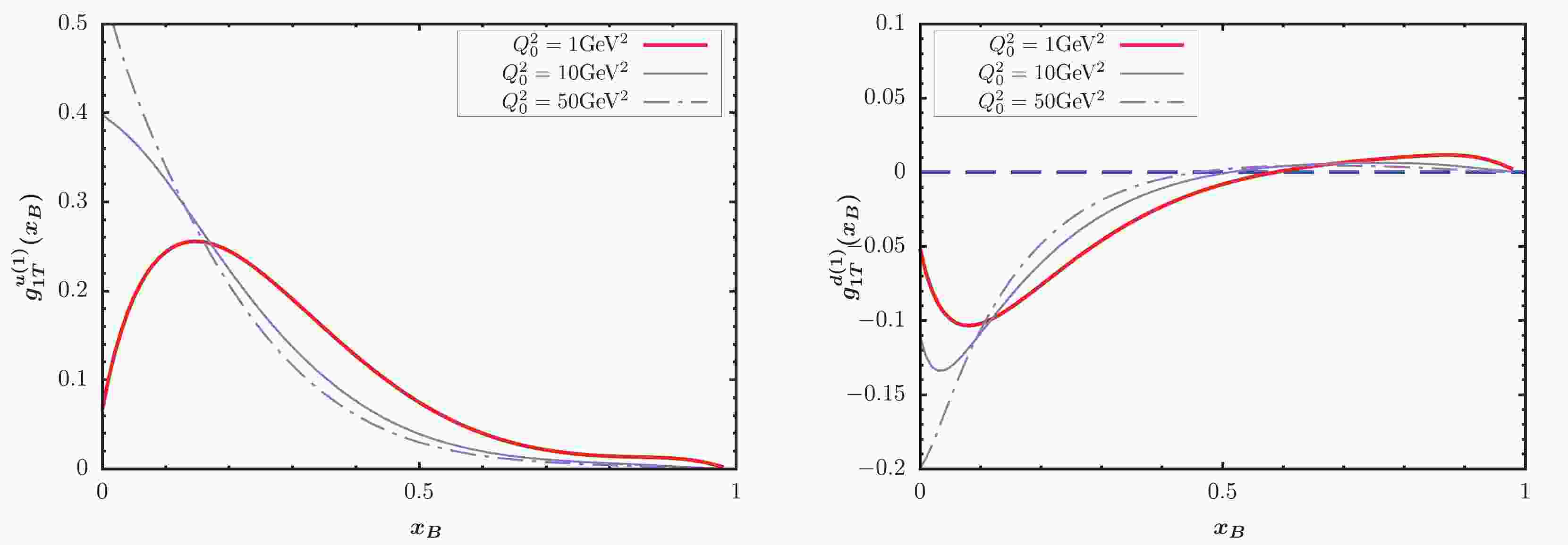
We used the QCDNUM evolution package [46] to obtain the numerical solution of the $\tilde{g}(x)$ evolution equation, where the scale evolution of the unpolarized fragmentation function was performed using the internal time-like evolution. We modified the original code of QCDNUM to add the evolution kernel of the $\tilde{g}(x)$ function, selecting the initial scale $Q_0^2 = 1$ GeV$^2$ for the evolution. Among the QCDNUM codes, we used the two loop QCD coupling constant [64], and the QCDNUM code was executed with the alignment $\alpha_s(Q_0) = 0.327$. In Fig. 1, we plot the $g_{1T}^{(1)}$ distributions of up and down quark at three scales. In both panels, the red solid lines depict the results at the initial scale $Q_0^2 = 1$ GeV$^2$, and the purple solid and dotted lines show the results at $Q_0^2 = 10$ GeV$^2$ and $Q_0^2 = 50$ GeV$^2$ after applying the evolution equation for $\tilde{g}$. We observe that the evolution equation significantly changes the shape and size of the TMD at different scales. The absolute maximum of TMD increases as the scale increases in both up and down quark cases.

Figure 1.  (color online) $g_{1T}^{(1)}$ distributions of up and down quark as a function of $x_B$.

To perform numerical calculations for $A_{LT}^{\cos(\phi_h-\phi_S)}$ in SIDIS at HERMES, we adopt the following kinematical cuts [65]

where W is the invariant mass of the photon-nucleon system, and $W^2 = (P+q)^2 \approx \dfrac{1-x_B}{x_B}Q^2$. Moreover, to apply TMD factorization and be consistent with Ref. [35], we select $P_{h\perp} \leqslant 0.6$ GeV for the produced hadron in SIDIS process at HERMES kinematics since we focus on the TMD factorization region $P_{h\perp} \leqslant Q$. At COMPASS kinematics, we select [33]

Additionally, we now make some predictions for the KM effect at EIC and EicC kinematics. For EIC, we adopt the following kinematics [66]

and for EicC, we adopt

In Figs. 2-8, we show the results for pion and kaon production. By integating over the other variables, the $x_B$-, $z_h$-, and $P_{h\perp}$-dependent KM effect are depicted in the left, central, and right panels of the figure, respectively. The solid lines represent our model predictions. The full circles with error bars show the preliminary HERMES and COMPASS data for comparison. For $\pi^-$ and $\pi^0$ production, Figs. 3-4 provide a good description for the HERMES data, while Fig. 2 somewhat overestimates the HERMES data. For pion production in Figs. 2-4, the obtained $P_{h\perp}$-dependent effects increase as $P_{h\perp}$ increases, and the largest effect can occur at 0.15. Note that this behavior does not mean that the asymmetries will tend to 1 as $P_{h\perp}$ increases. If we loosen the constraint $P_{h\perp}<0.6$ GeV by applying $P_{h\perp}<1$ GeV, the $P_{h\perp}$-distribution in, e.g., Fig. 2 will become very large at approximately $P_{h\perp} = 0.7$ GeV. The reason is that the model predicted denominator of the asymmetry decreases to zero at approximately $P_{h\perp} = 0.7$ GeV. Thus, such model behavior indirectly proves the necessity for adopting $P_{h\perp}<0.6$ GeV to guarantee TMD factorization. A similar behavor is observed for $P_{h\perp}$-distribution in similar model calculations, e.g., [39, 40]. For the $K^+$ production, the obtained asymmetries in Fig. 5 also exhibit a similar result with the HERMES data. The $P_{h\perp}$-dependent effect in Fig. 5 can reach nearly 0.1 at the point with $x_B = 0.5$. Fig. 6 indicates rather small effects for $K^-$ production, which is also basically consistent with HERMES data. Note that when $x_B > 0.5$, the predicted $z_h$-dependent effect nearly becomes zero. In Figs. 7 and 8, we plot the TMD predictions of the KM effect for $\pi^+,\pi^-$ production. The cases are similar to those of HERMES, and the predictions are basically consistent with COMPASS data. The uncertainty may resuslt from $f_1$,$D_1$,$\tilde{g}$, the evolution kernel of $\tilde{g}$, and the nonperturbative factors. Overall, the TMD effects are non-negligible and ocassionally significant.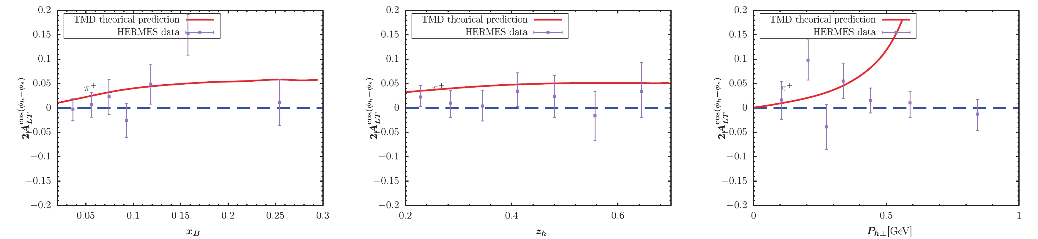

Figure 2.  (color online) KM effect calculated within TMD factorization compared with the HERMES measurement [65] for $\pi^+$ production.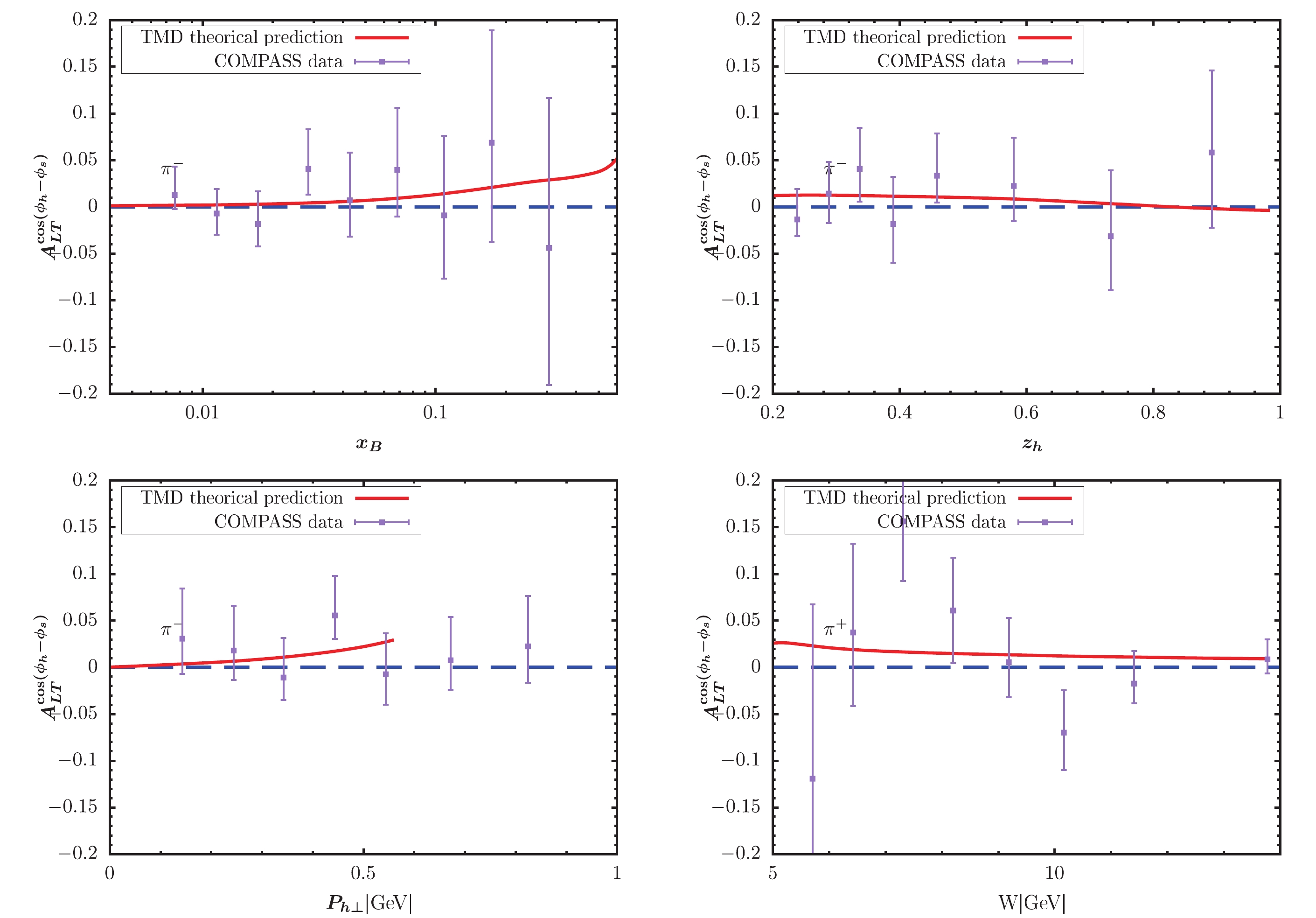

Figure 8.  (color online) KM effect calculated within TMD factorization compared with the COMPASS measurement [33] for $K^-$ production.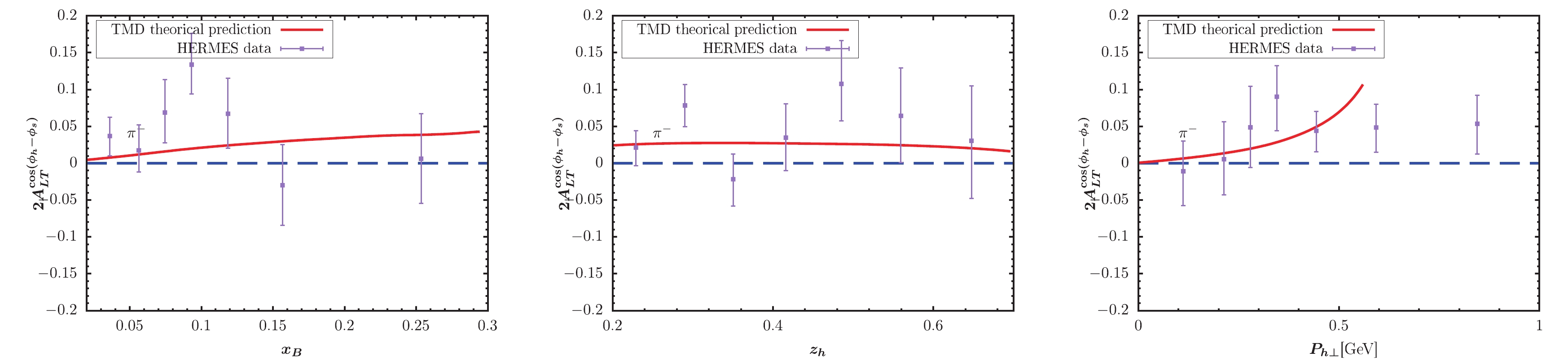

Figure 3.  (color online) KM effect calculated within TMD factorization compared with the HERMES measurement [65] for $\pi^-$ production.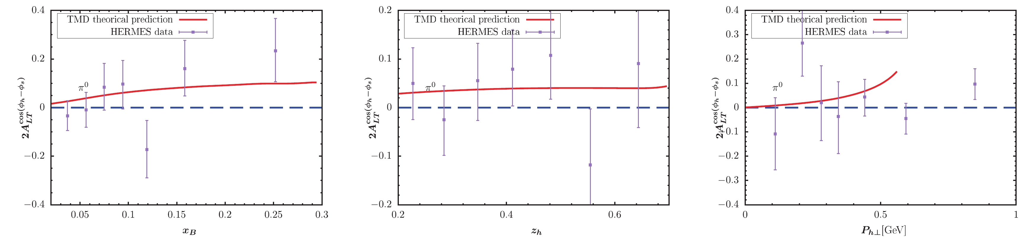

Figure 4.  (color online) KM effect calculated within TMD factorization compared with the HERMES measurement [65] for $\pi^0$ production.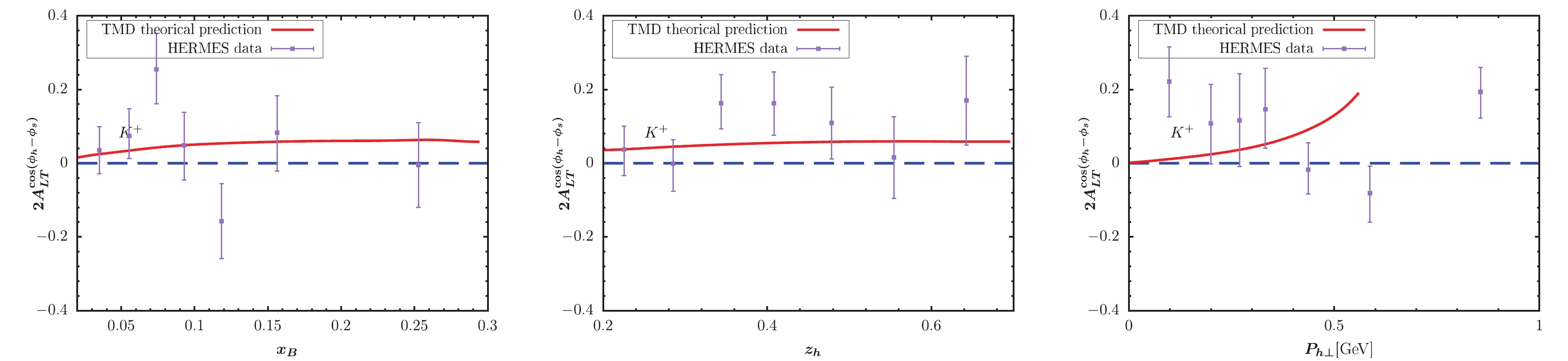

Figure 5.  (color online) KM effect calculated within TMD factorization compared with the HERMES measurement [65] for $K^+$ production.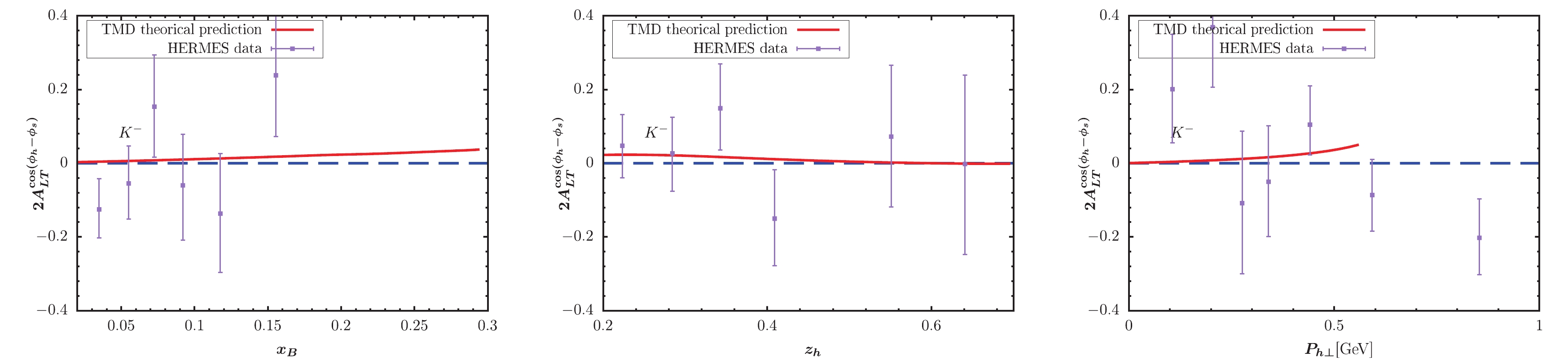

Figure 6.  (color online) KM effect calculated within TMD factorization compared with the HERMES measurement [65] for $K^-$ production.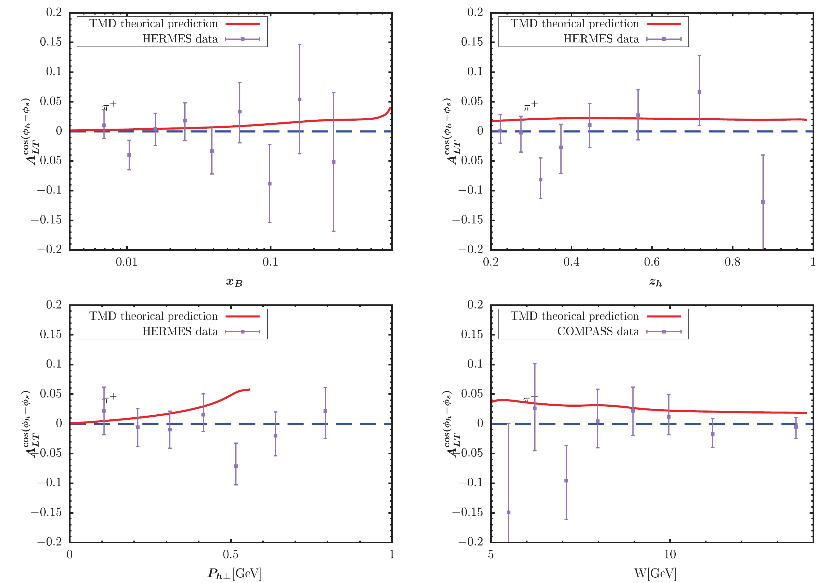

Figure 7.  (color online) KM effect calculated within TMD factorization compared with the COMPASS measurement [33] for $K^-$ production.

Figs. 9-12 also show similar asymmetry results for kaon production at EIC and EicC kinematics. By integating over the other variables, the $x_B$-, $z_h$-, and $P_{h\perp}$-dependent KM effect are depicted in the left, central, and right panels of the figure, respectively. We observe that the KM effect results for $K^+$ production are larger than those for $K^-$ production. Generally, the KM effect results at EicC kinematics are slightly larger than those at EIC kinematics, and shapes of $x_B$-, $z_h$-, and $P_{h\perp}$-dependent KM effects at both EIC and EicC kinematics are similar. Future experiments will be useful for extracting the KM function after a global analysis of data sets.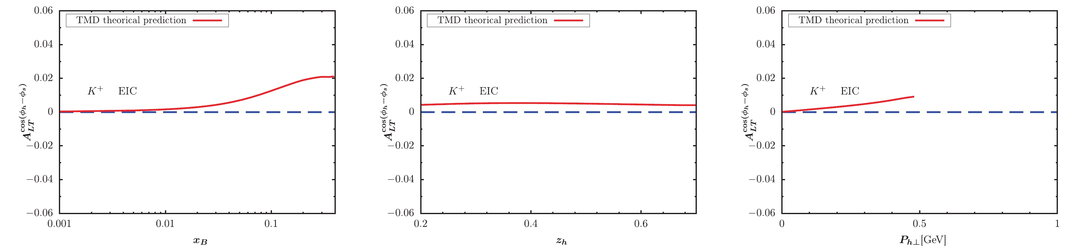

Figure 9.  (color online) KM effect calculated within TMD factorization for $K^+$ production at EIC kinematics.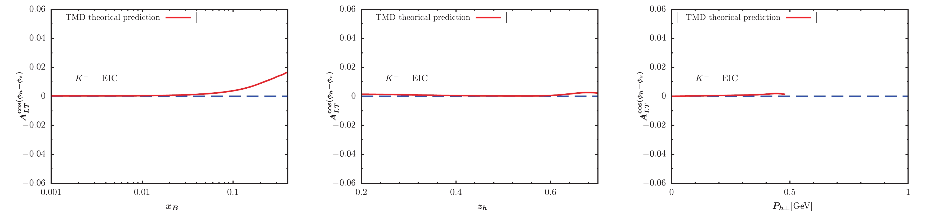

Figure 10.  (color online) KM effect calculated within TMD factorization for $K^-$ production at EIC kinematics.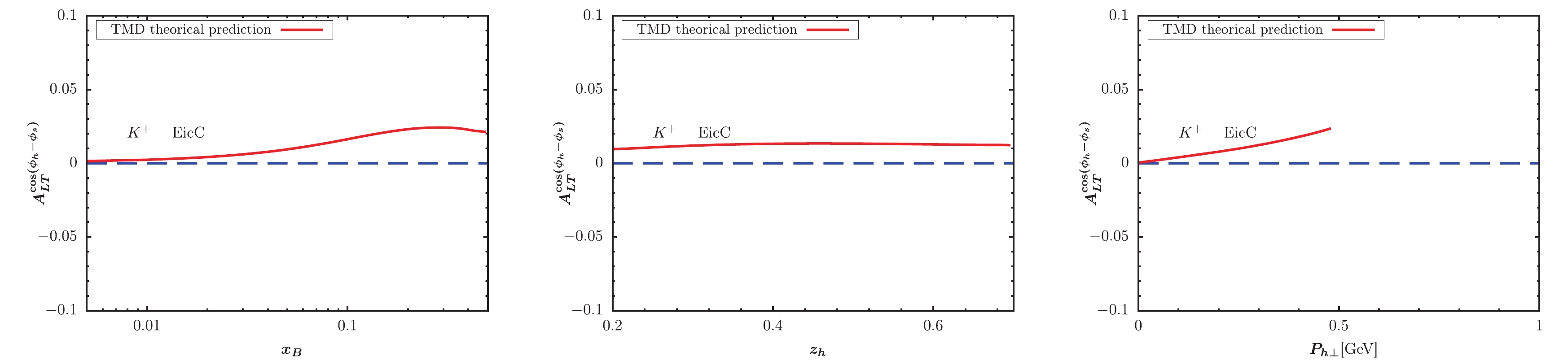

Figure 11.  (color online) KM effect calculated within TMD factorization for $K^+$ production at EicC kinematics.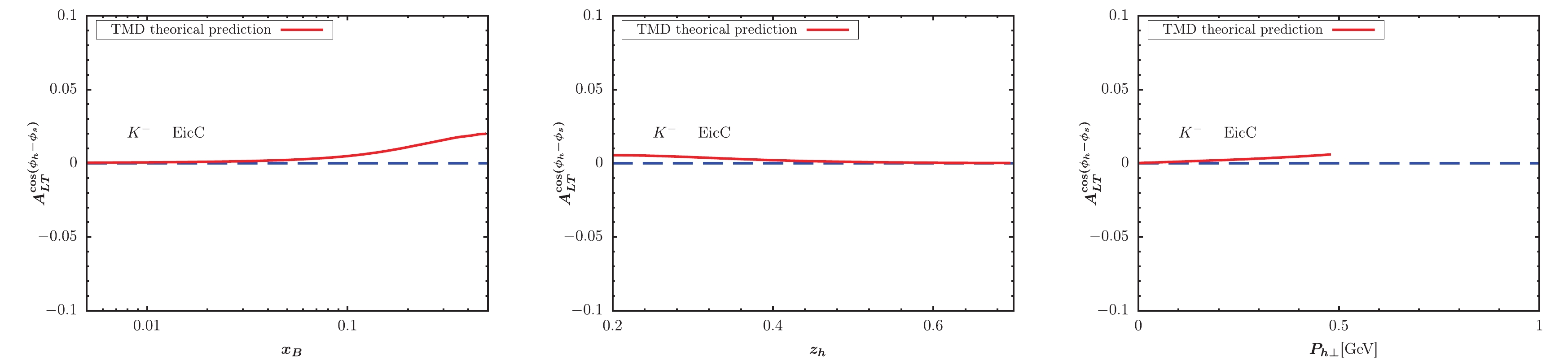

Figure 12.  (color online) KM effect calculated within TMD factorization for $K^-$ production at EicC kinematics.

In this study, we investigated the KM effect in the SIDIS process within the framework of TMD factorization. We considered the TMD evolution of $\tilde{g}$ and unpolarized parton distribution and fragmentation functions. We first obtain a previous parametrization of $\tilde{g}$ function at a initial energy $Q_0$ and then evolve it to the CSS default initial scale $\mu_b$ through an approximation evolution kernel, which includes only the homogenous terms for the $\tilde{g}$ function. Subsequently, we obtain the $x_B$-, $z_h$-, and $P_{h\perp}$-dependent KM effects in SIDIS for the pion and kaon production at the HERMES and COMPASS kinematics. The numerical results are compared with the corresponding HERMES and COMPASS measurements. We observe that the KM effect within the TMD factorization and evolution in the corresponding kinematics is basically consistent with the HERMES and COMPASS measurements. The TMD effect is occasionally significant.