


 Abstract
 HTML
HTML Reference
 Related
 PDF
PDF


-
The study of nuclear structure is a field facing great opportunities and challenges in recent years, and its goal is to establish a comprehensive microscopic theoretical framework [1, 2]. To achieve this goal, several physical models have been proposed, which can be divided into several different approaches: the
$ ab $ $ initio $ methods [3, 4], shell model calculation [5], self-consistent mean-field theory [6, 7], and macroscopic models with quantum shell corrections [8]. In the past few decades, numerous nuclear structure theories have extended from stable nuclei to exotic nuclei [9, 10]. Compared with stable nuclei, there are novel phenomena such as neutron halo, neutron skin, giant resonance, and super deformation in exotic nuclei, which pose serious challenges to the nuclear structure model [11, 12]. Therefore, it is particularly important to construct a theoretical nuclear structure model to explain the macroscopic and microscopic phenomena in both stable and exotic nuclei.Among a number of nuclear structure models, the self-consistent mean-field theory is a comprehensive and successful model that is widely used for studying the nuclear structure for both stable and exotic nuclei [13, 14]. The mean-field model incorporates the effective potential and the pairing field [6]. There are two main ways to construct the mean-field model: relativistic and non-relativistic methods. For the relativistic method [15], the interaction between nucleons is transmitted through the meson fields, while the non-relativistic method [16] provides the nucleon-nucleon interactions directly. Regarding the global properties of the nuclei, the two classes of mean-field models provide similar descriptions, and both are consistent with the experimental data, such as the binding energies and charge radii [17-19]. However, while the global properties can only reflect the superposition of all nucleons, there are still some differences between these two models in describing the properties of the single nucleon. Thus, it is significant to find a suitable experimental observation to analyze the validity of the single-particle wave functions obtained with the relativistic and non-relativistic mean-field models.
Electron scattering is an accurate tool to explore the electromagnetic properties of nuclei, which can help in the deep understanding of the nuclear charge and current distributions [20-22]. For the odd-A nuclei, because the angular momentum of all nucleons expect the valence nucleon is paired, the total angular momentum of these nucleons is zero, which has no contribution to the magnetic properties. Therefore, the magnetic moment of the odd-A nuclei is determined to a great extent by the unpaired nucleon [23-25]. Compared with elastic Coulomb electron scattering, which can measure the total nuclear charge density distributions [26-30], magnetic electron scattering provides a direct way to explore the properties of the single nucleon [31-33]. In elastic magnetic electron scattering, the most important observable is the magnetic form factors
$ |F_\mathrm{M}(q)|^{2} $ , which is closely related to the magnetic moment [34, 35]. In addition, the orbitals of the valence nucleons can be directly reflected by the magnetic form factors.In the last few years, there have been several significant and instructive calculations of the magnetic form factors within different theoretical frameworks [36-41], including the relativistic mean-field (RMF) and non-relativistic Skyrme Hartree-Fock (SHF) for both the spherical and deformed cases [42-46]. Because different nuclear structure models provide different descriptions of the nuclear single-particle properties, it is necessary to perform a comparative study on the magnetic scattering processes. The results can provide useful information for further analyzing the effectiveness of nuclear structure models.
By comparing the magnetic form factors calculated using the RMF and SHF models, the aim of this study is to systematically analyze the properties of single-particle described by these two models. Both stable and exotic nuclei, namely,
$ {}^{11} {\rm{B}}$ ,$ {}^{17} {\rm{O}}$ ,$ {}^{27} {\rm{Al}}$ ,$ {}^{41} {\rm{Ca}}$ ,$ {}^{57} {\rm{Ti}}$ ,$ {}^{59} {\rm{Co}}$ ,$ {}^{115} {\rm{In}}$ , and$ {}^{132} {\rm{Sn}}$ , are selected. First, we focus our studies on the single-particle properties of odd-A nuclei based on different models. For the non-relativistic SHF model, by solving the Hartree-Fock equations for Skyrme's interaction, the single-particle wave functions can be obtained. For the relativistic mean-field model, the four-component Dirac spinor wave functions can be obtained by solving the Dirac and Klein-Gordon equations simultaneously. Second, we construct the theoretical frameworks of non-relativistic and relativistic magnetic electron scattering. The spherical limit method is used to calculate$ |F_\mathrm{M}(q)|^{2} $ , which provides an efficient tool for describing the electromagnetic transitions of spherical and deformed cases in a unified fashion. Third, based on the different types of wave functions obtained from the RMF and SHF models, the magnetic form factors of the selected nuclei are obtained and compared with the experimental data. For the deformed nuclei, geometrical factors are introduced to consider the influences of deformation on$ |F_\mathrm{M}(q)|^{2} $ . A clear improvement in the agreement between the theoretical results and experimental data can be observed. To understand the structure of the exotic region, the magnetic form factors$ |F_\mathrm{M}(q)|^{2} $ of unstable nuclei are also studied. The differences in the descriptions of the single-particle orbital between the RMF and SHF models are reflected from$ |F_\mathrm{M}(q)|^{2} $ . In particular, in the high-momentum transfer, the differences are amplified by the angular momentum-dependent term in the matrix element; therefore, this region is ideal to study the differences between the two models.This paper is organized as follows. In Section II, the theoretical frameworks of magnetic electron scattering and deformed formalism are provided. In Section III, the results and discussions about
$ |F_\mathrm{M}(q)|^{2} $ for both stable and exotic nuclei are presented. Finally, Section IV concludes the paper. -
In this section, the theoretical frameworks for studying the magnetic form factors
$ |F_\mathrm{M}(q)|^{2} $ of both spherical and deformed nuclei are presented. First, we discuss magnetic electron scattering in the non-relativistic framework. Then, we further investigate$ |F_\mathrm{M}(q)|^{2} $ under the relativistic framework. Finally, the influences of the deformation effect on$ |F_\mathrm{M}(q)|^{2} $ are considered. -
In the Skyrme Hartree-Fock calculation under spherical symmetry, the single-particle wave function can be written as [47]
$ \Phi_{i}({\vec{r}},{{\sigma}},{\tau}) = \dfrac{R_{\alpha}(r)}{r} {\cal{Y}}_{l,j,m}({\hat{r}},{\sigma}) \chi_{\bar{q}}({\tau}), $

(1) where
$ {\cal{Y}}_{l j m}(\hat{r}, \sigma) = \sum\limits_{m_{l} m_{s}}\langle l \frac{1}{2} m_{l} m_{s} \mid j m\rangle Y_{l m_{l}}(\theta,\varphi) \chi_{m_{s}}(\sigma), $

$ R_{nl} $ is the radial wave function, and$ \chi_{\bar{q}}({\tau}) $ is the isospin spinor. The index i represents the set of quantum numbers: the angular momentum l, the total angular momentum j, the magnetic quantum number m, the charge q, and the principal quantum number n. The notation$ \alpha = \left\{q, n, l, j\right\} $ is also introduced for simplicity.In the plane-wave Born approximation (PWBA) [48], the cross section of the elastic magnetic electron scattering can be expressed as
$ \frac{{\rm d} \sigma}{{\rm d} \Omega} = \sigma_\mathrm{M}\left(\frac{1}{2}+\operatorname{tan}^{2} \frac{\theta}{2}\right) \left|F_{\mathrm M}(q)\right|^{2}, $

(2) where
$ \sigma_\mathrm{M} = \left(\dfrac{\alpha \cos \frac{\theta}{2}}{2 E \sin ^{2} \frac{\theta}{2}}\right)^{2} $ is the Mott cross section. The total magnetic form factor$ \left|F_{\mathrm M}(q)\right|^{2} $ can be expressed as the sum of the Lth magnetic form factor$ \left|F^{\mathrm {mag}}_{L}(q)\right|^{2} $ ,$ \left|F_{\mathrm M}(q)\right|^{2} = \sum\limits_{L = 1}^{\mathrm {odd}} \left|F^{\mathrm {mag}}_{L}(q)\right|^{2}. $

(3) With the transverse magnetic multipole operator
$ T_{L}^\mathrm{m a g} $ , the Lth magnetic form factor is defined as$ F_{L}^\mathrm{mag}(q) = \sqrt{\frac{4 \pi}{2 J_{i}+1}}\left|\left\langle J_{f}\left\|T_{L}^\mathrm{m a g}\right\| J_{i}\right\rangle\right|. $

(4) We note that in the PWBA framework, the magnetic form factor in Eq. (4) can be deduced as the Fourier transform of the transition current density
$ J_{L L}(r) $ ,$ F_{L}^\mathrm{mag}(q) = \int_{0}^{\infty} J_{L L}(r) j_{L}(q r) r^{2} {\rm d} r. $

(5) The transition current density
$ J_{L L}(r) $ consists of two parts [49]:$ J_{L L}(r) = J_{L L}^\mathrm{c}+J_{L L}^\mathrm{s}. $

(6) $ \begin{aligned}[b] J_{LL}^{\rm{c}}(r) =& \frac{{{\rm i}e}}{M}{( - 1)^{j - 1/2}}{g_l}(2L + 1)(2l + 1)(2j + 1)\\ & \times {\left( {\frac{{(2L - 1)l(l + 1)(2l + 1)}}{{4\pi (L + 1)}}} \right)^{1/2}}\\ & \times \left\{ {\begin{array}{*{20}{c}} l&j&{1/2}\\ j&l&L \end{array}} \right\}\left\{ {\begin{array}{*{20}{c}} {L - 1}&1&L\\ l&l&l \end{array}} \right\}\\ &\times \left( {\begin{array}{*{20}{c}} l&{L - 1}&l\\ 0&0&0 \end{array}} \right)\frac{{R_{nl}^2(r)}}{r}, \end{aligned} $

(7) $ \begin{aligned}[b] J_{L L}^\mathrm{s}(r) =& -{\rm i}\left[\frac{L^{1 / 2}}{\hat{L}}\left(\frac{\rm d}{{\rm d} r}+\frac{L+2}{r}\right) \mu_{s L L+1}(r)\right.\\ &\left.+\frac{(L+1)^{1 / 2}}{\hat{L}}\left(\frac{\rm d}{{\rm d} r}-\frac{L-1}{r}\right) \mu_{s L L-1}(r)\right], \end{aligned} $

(8) $ \begin{aligned}[b] {\mu _{sL{L^\prime }}}(r) =& \frac{e}{{2M}}{( - 1)^l}{\mu _i}(2l + 1)(2j + 1)\\ & \times {\left( {\frac{{6(2L + 1)\left( {2{L^\prime } + 1} \right)}}{{4\pi }}} \right)^{1/2}}\\ &\times \left\{ {\begin{array}{*{20}{c}} l&l&{{L^\prime }}\\ {1/2}&{1/2}&1\\ j&j&L \end{array}} \right\}\left( {\begin{array}{*{20}{c}} l&{{L^\prime }}&l\\ 0&0&0 \end{array}} \right)R_{nl}^2(r), \end{aligned} $

(9) where
$ R_{n l} $ is the radial wave function of the valence nucleon in Eq. (1), and$ \hat{L} = \sqrt{2 L+1} $ . The convective current$ J_{L L}^\mathrm{c} $ is generated by the orbital motion of protons and$ J_{L L}^\mathrm{s} $ is produced by the spin of protons and neutrons.In this study,
$ R_{n l} $ is calculated using the SHF model with the SLY4 parameter set [50]. For a neutron, the Lande factor$ g_{ l} = 0 $ and the magnetic moment$ \mu_{ i} = -1.913 $ . For a proton, the Lande factor$ g_{ l} = 1 $ and the magnetic moment$ \mu_{ i} = 2.793 $ . By substituting Eqs. (6) - (9) into Eq. (5), we can obtain the magnetic form factor in the non-relativistic framework. -
In the relativistic theory of magnetic electron scattering, the single-particle wave function of the valence nucleon is expressed as
$ \begin{aligned}[b] {\psi _{n\kappa m}} =& \left[ {\begin{array}{*{20}{c}} {{\rm i}[G(r)/r]{\Phi _{\kappa m}}(\hat r)}\\ { - [F(r)/r]{\Phi _{ - \kappa m}}(\hat r)} \end{array}} \right] = \left[ {\begin{array}{*{20}{c}} {{\rm i}|n\kappa m\rangle }\\ { - \overline {|n\kappa m\rangle } } \end{array}} \right]\\ = &\left[ {\begin{array}{*{20}{c}} {{\rm i}\left| {nl\dfrac{1}{2}jm} \right\rangle }\\ { - \left| {nl'\dfrac{1}{2}jm} \right\rangle } \end{array}} \right], \end{aligned} $

(10) through the selection of this phase factor in Eq. (10), the upper and lower components
$ G(r) $ and$ F(r) $ are real-valued functions. The angular quantum number κ determines the total and the orbital angular momentum quantum numbers l,$ l' $ and j,$ j = |\kappa|-\frac{1}{2}, $

(11) $ \begin{array}{*{20}{l}} {l = \kappa ,}&{{l^\prime } = l - 1,}&{(\kappa > 0),}\\ {l = - (\kappa + 1),}&{{l^\prime } = l + 1,}&{(\kappa < 0).} \end{array}$

(12) In the independent single-particle shell-model, only the unpaired valence nucleon can contribute to the magnetic form factors. The elastic magnetic form factors squared are expressed as follows:
$ |F_{\mathrm{M}}(q)|^{2} = \frac{4 \pi f_{s n}^{2}(q) f_{c m}^{2}(q)}{2 J_{i}+1} \sum\limits_{L = 1}^{\text {odd }}|\langle J_{f}\|\hat{T}_{L}^{\rm{mag}}\| J_{i}\rangle|^{2}. $

(13) In previous studies [51-54], it has been shown that the neutron densities, spin-orbit densities, and center-of-mass correction have significant contributions to the nuclear charge radius. The contribution of the nucleon magnetic form factor and center-of-mass corrections to
$ |F_{\mathrm{M}}(q)|^{2} $ are also taken into account in our studies. The center-of-mass factor [55] in Eq. (13) is given by$ f_{c m}(q) = \mathrm{exp}( q^{2}b^{2} /4A $ ), where the oscillator parameter b is often considered as$ b = A^{1/6} $ fm−1. The single-nucleon magnetic form factor for protons and neutrons is given by$ f_{s n}(q) = \frac{1}{\left(1+r_{p}^{2} q^{2} / 12\right)^{2}}, $

(14) with
$ r_{p} = 0.81 $ fm.The multipole operator
$ \hat{T}_{L \mu}^{\rm{mag}} $ is written as [23, 49]$ \hat{T}_{L \mu}^\mathrm{m a g}(q) = \int j_{L}(q r) Y_{L L}^{\mu}(\hat{r}) \cdot \hat{J}(r) {\rm d}^{3} r, $

(15) and
$ \langle J_{f}\|\hat{T}_{L}^{\mathrm{mag}}(q)\| J_{i}\rangle $ is the reduced matrix element of the multipole operator. The vector spherical harmonics$ Y_{L L}^{\mu}(\hat{r}) $ are defined as$ {\boldsymbol{Y}}^{\mu}_{\lambda \lambda^{\prime} }(\hat{r}) = \sum\limits_{\alpha, \beta} Y_{\lambda^{\prime} \alpha}(\hat{r})\left\langle\lambda^{\prime} \alpha 1 \beta \mid \lambda^{\prime} 1 \lambda \mu\right\rangle \hat{e}_{\beta}. $

According to the Wigner-Eckart theorem, the subscript µ of Eq. (15) has been reduced, and we can obtain the reduced matrix elements
$ \begin{aligned}[b] \langle J_{f}\|\hat{T}_{L}^{\mathrm{mag}}(q)\| J_{i}\rangle = & -(q / 2 M_{n})\langle n \kappa\|\lambda \Sigma_{L}^{\prime \mu }\| n \kappa\rangle\\ &+\left(q / 2 M_{n}\right) \overline{\langle n \kappa \|} \lambda\Sigma_{L}^{\prime \mu} \overline{\| n \kappa\rangle} \\&+2 \overline{\langle n \kappa \|} Q \Sigma_{L}^{\mu } \| n \kappa\rangle, \end{aligned}$

(16) where Q,
$ M_{n} $ are the electric charge, mass of the nucleon and λ is the anomalous magnetic moment, for proton$ \lambda_{p} = \mu_{ p} - 1 $ , and for neutron$ \lambda_{n} = \mu_{ n} $ . The operators$ \Sigma_{L}^{ \mu} $ and$ \Sigma_{L}^{\prime \mu} $ are given by$ \Sigma_{L}^{\mu}(r) \equiv M_{L L}^{\mu}(r) \cdot \sigma, $ $\Sigma_{L}^{\prime \mu}(r) \equiv $ $ -i\left[\nabla \times M_{L L}^{\mu}(r)\right] \cdot \sigma / q, $ $ \; M_{L L}^{\mu}(r) \equiv j_{L}(q r) Y_{L L}^{\mu}(\hat{r}) $ .The integral expressions in Eq. (16) can be written in the following form
$ \begin{aligned}[b] \left\langle {n\kappa \left\| {\Sigma _L^{\prime \mu }} \right\|n\kappa } \right\rangle =& \frac{{{{( - 1)}^{l + 1}}}}{q}{\left( {\frac{6}{{4\pi }}} \right)^{1/2}}(2l + 1)(2j + 1) \times \left[ {\left\{ {\begin{array}{*{20}{c}} l&{\;l}&{L + 1}\\ {\dfrac{1}{2}}&{\;\dfrac{1}{2}}&1\\ j&{\;j}&L \end{array}} \right\}\left( {\begin{array}{*{20}{c}} l&{\;L + 1}&{\;l}\\ 0&{\;0}&{\;0} \end{array}} \right)}\right.{{\big[L(2L + 3)\big]}^{1/2}} \\ & \times \int {{j_L}} (qr){g^2}(r)\left(\frac{\rm d}{{{\rm d}r}} + \frac{{L + 2}}{r}\right){r^2}{\rm d}r - \left\{ {\begin{array}{*{20}{c}} l&{\;l}&{\;L - 1}\\ {\dfrac{1}{2}}&{\;\dfrac{1}{2}}&1\\ j&{\;j}&{\;L} \end{array}} \right\}\left( {\begin{array}{*{20}{l}} l&{\;L - 1}&{\;l}\\ 0&{\quad \;0}&{\;0} \end{array}} \right)\times {\big[(L + 1)(2L - 1)\big]^{1/2}}\\&\left. { \times \int {{j_{L - 1}}} (qr){g^2}(r){r^2}{\rm d}r} \right], \end{aligned} $ 
(17) $ \begin{aligned}[b] \overline {\langle n\kappa ||} \Sigma _L^{\prime \mu }\overline {||n\kappa \rangle } =& \frac{{{{( - 1)}^{{l^\prime } + 1}}}}{q}{\left( {\frac{6}{{4\pi }}} \right)^{1/2}}\left( {2{l^\prime } + 1} \right)(2j + 1) \times \left[ {\left\{ {\begin{array}{*{20}{c}} {{l^\prime }}&{\;{l^\prime }}&{\;L + 1}\\ {\dfrac{1}{2}}&{\;\dfrac{1}{2}}&{\;1}\\ j&{\;j}&{\;L} \end{array}} \right\}\left( {\begin{array}{*{20}{l}} {{l^\prime }}&{\;L + 1}&{\;{l^\prime }}\\ 0&{\quad \;0}&{\;0} \end{array}} \right)} \right.\\ & \times {[L(2L + 3)]^{1/2}} \times \int {\rm d} r{r^2}{j_L}(qr)\left(\frac{\rm d}{{{\rm d}r}} + \frac{{L + 2}}{r}\right){f^2}(r) + \left\{ {\begin{array}{*{20}{c}} {{l^\prime }}&{\;{l^\prime }}&{\;L - 1}\\ {\dfrac{1}{2}}&{\;\dfrac{1}{2}}&{\;1}\\ j&{\;j}&{\;L} \end{array}} \right\}\left( {\begin{array}{*{20}{l}} {{l^\prime }}&{\;L - 1}&{\;{l^\prime }\;}\\ 0&{\quad \;0}&{\;0} \end{array}} \right)\\ & \times {[(L + 1)(2L - 1)]^{1/2}}\left. { \times \int {\rm d} r{r^2}{j_L}(qr)\left(\frac{\rm d}{{{\rm d}r}} - \frac{{L - 1}}{r}\right){f^2}(r)} \right], \end{aligned} $

(18) $ \begin{aligned}[b] \overline {\langle n\kappa ||} \Sigma _L^\mu ||n\kappa \rangle =& {( - 1)^{{l^\prime }}}{\left( {\frac{6}{{4\pi }}} \right)^{1/2}}(2L + 1)(2j + 1){\left[ {(2l + 1)\left( {2{l^\prime } + 1} \right)} \right]^{1/2}} \times \left\{ {\begin{array}{*{20}{l}} {{l^\prime }}&{\;l}&{L\;}\\ {\dfrac{1}{2}}&{\;\dfrac{1}{2}}&{\;1}\\ j&{\;j}&{\;L} \end{array}} \right\}\left( {\begin{array}{*{20}{l}} {{l^\prime }}&{\;L}&{\;l}\\ 0&{\;0}&{\;0} \end{array}} \right)\int {\rm d} r{r^2}{j_L}(qr)g(r)f(r), \end{aligned}$

(19) where
$ g(r) = G(r)/r $ , and$ f(r) = F(r)/r $ . To calculate the magnetic form factors, we use the RMF model to obtain the wave functions in the present research. The values of the matrix elements in Eq. (16) mainly come from the contributions of the upper components of the RMF wave functions in Eq. (17). The contributions of the lower component in Eq. (18) and the crossed term in Eq. (19) to the magnetic form factors are minuscule. -
In elastic scattering, the initial and final states in Eq. (4) are consistent. The deformed magnetic multipole form factors [31, 56, 57] can be expressed as the intrinsic form factors weighted by the angular momentum correlation coefficient
$ \begin{aligned}[b] \left.{F}_{L}^{\mathrm{mag}}\right|_{\text {def }} =& \langle k k L 0 \mid k k\rangle {\cal{F}}_{L k}^{\mathrm {mag}}+\langle k-k\,L\,2 k \mid k k\rangle {\cal{F}}_{L 2 k}^{ \mathrm {mag}} \\ &+\frac{L(L+1)}{\sqrt{2}}\langle k k L 0 \mid k k\rangle {\cal{F}}_{L R}^{\mathrm {mag}}, \end{aligned} $

(20) where
$ {\cal{F}}_{LR}^{\mathrm{ mag}} $ are the transverse multipoles of the collective rotational current, which are related the the nuclear rotation model describing the energy band. For different microscopic and macroscopic models, the expressions for$ {\cal{F}}_{LR}^{\mathrm{ mag}} $ can be found in [58]. The single-particle multipoles$ {\cal{F}}_{L k}^{\mathrm {mag}} $ and$ {\cal{F}}_{L 2k}^{\mathrm {mag}} $ are determined by the single-particle wave function of the valence nucleon [44],$ {\cal{F}}_{L k}^{\mathrm {mag}} = \left< \phi _k \right|\hat{T}_{L0}^{\mathrm {mag}}\left|\phi_{k} \right>, $

(21) $ {\cal{F}}_{L 2 k}^{\mathrm {mag}} = \left< \phi _k |\hat{T}_{L 2k}^{ \mathrm {mag}}|\phi_{\bar{k}} \right> +\delta_{k, 1 / 2} \frac{a}{\sqrt{2}} {\cal{F}}_{L R}^{\mathrm {mag}}, $

(22) where
$ \hat{T}_{L \mu}^{\mathrm {mag}} $ is the multipole operator [49], as in Eq. (15). In addition,$ \phi_{\bar{k}} $ is the time reverse of the wave function of the odd nucleon.With the deformed intrinsic wave function
$ \phi_{k} $ calculated from the axially deformed mean-field models, the matrix elements of the magnetic multipole operators in Eq. (21) and Eq. (22) can be determined. In this study, we construct the matrix elements under the condition of the spherical limit, which are evaluated in terms of the overlaps of the mean-field intrinsic deformed wave functions. The spherical limit method [59, 60] provides an efficient tool for describing the electromagnetic transitions of the spherical and deformed cases in a unified fashion, which has been proved to be identical to the complete deformed calculations in Eq. (21) and Eq. (22).In the spherical limit, the collective magnetic multipoles are zero, and the single-particle wave function
$ \phi_{{k}} $ involves a single angular momentum component$ \phi_{{jj}} $ . In this case$ j = k = J_{i} $ , and the intrinsic form factors can be obtained using the Wigner-Eckart theorem,$ \begin{aligned}[b] {\cal{F}}_{L k}^{\mathrm {mag}} =& \left< \phi_{j j}\right|\hat{T}_{L 0}^{\mathrm {mag}}\left| \phi_{j j}\right>\\ = &\frac{1}{\sqrt{2 j+1}}\langle j j L 0 \mid j j\rangle \langle \phi_{j}\|\ \hat{T}_{L }^{\mathrm {mag}}\| \phi_{j}\rangle, \end{aligned} $

(23) $ \begin{aligned}[b] {\cal{F}}_{L 2k}^{\mathrm{mag}} =& \left< \phi_{j j}|\hat{T}_{L 2j}^{\mathrm {mag}}| \bar{\phi}_{j j} \right>\\ =& \frac{({-1})^{L}}{\sqrt{2 j+1}}\langle j-j\,L\,2j \mid j j\rangle \langle \phi_{j}\|\ \hat{T}_{L }^{\mathrm {mag}}\| \phi_{j}\rangle,\\ \end{aligned} $

(24) where
$ \phi_{j} $ is the single-particle wave function from the spherical mean-field models.The
$ \left.{F}_{L}^{\mathrm{mag}}\right|_{\mathrm{sph}} $ is the magnetic form factor of the spherical case, which is given by Eq. (4) and Eq. (13) for the non-relativistic and relativistic frameworks, respectively. Substituting Eq. (23) and Eq. (24) into Eq. (20), we can obtain the relation between$ \left.{F}_{L}^{\mathrm{mag}}\right|_{\mathrm{sph}} $ and$ \left.{F}_{L}^{\mathrm{mag}}\right|_{\mathrm{def}} $ ,$ \left.{F}_{L}^{\mathrm{mag}}\right|_{\text {def }} = \left.\eta_{j}^{L}\cdot {F}_{L}^{\mathrm{mag}}\right|_{\text {sph}}, $

(25) where the geometric factors
$ \eta_{j}^{L} $ can be expressed as$ \eta_{j}^{L} = \langle j j L 0 \mid j j\rangle^{2}\left[1+\delta_{L, 2 j} \frac{\langle j-j\,L\,2 j \mid j j\rangle^{2}}{\langle j j L 0 \mid j j\rangle^{2}}\right]. $

(26) Combining Eqs. (21) - (24), it can be seen that throughout the transformation from the deformed to the spherical limit, the loss of the favored intrinsic direction results in the geometric factor
$ \eta_{j}^{L} $ in Eq. (26), and the transition matrix elements are insensitive to the deformation parameter β. -
In this section, we present the nuclear ground-state properties, such as the root-mean-square (RMS) charge radii
$ R_{\mathrm{C}} $ [61], the valence nucleon RMS radii$ R_{\mathrm{V}} $ , and the binding energies per nucleon$ B/A $ [62], for both stable and exotic nuclei.$ ^{11} {\rm{B}}$ ,$ ^{17} {\rm{O}}$ ,$ ^{27} {\rm{Al}}$ ,$ ^{41} {\rm{Ca}}$ ,$ ^{57} {\rm{Ti}}$ ,$ ^{59} {\rm{Co}}$ ,$ ^{115} {\rm{In}}$ , and$ ^{133} {\rm{Sn}}$ are chosen as the candidates. The theoretical$ R_{\mathrm{C}} $ and$ B/A $ given in Table 1 are calculated from the RMF model with the NL-SH parameter set [63] and the SHF model with the SLY4 parameter set. It can be seen that both the RMF and SHF models can reproduce the ground-state properties of the nuclei, which proves the validity and suitability of these two models in describing the global properties of nuclei. The validity of the single-particle wave functions can be further discussed through$ |F_\mathrm{M}(q)|^{2} $ .Nuclei $ B/A $ /MeV

$ R_{\mathrm C} $ /fm

$ R_{\mathrm V} $ /fm

SHF RMF Expt. SHF RMF Expt. SHF RMF 11B 7.053 6.874 6.928 2.435 2.404 2.406 2.651 2.522 17O 7.899 7.755 7.751 2.723 2.698 2.693 3.409 3.399 27Al 8.295 8.127 8.332 3.101 2.995 3.061 3.394 3.267 41Ca 8.648 8.535 8.547 3.514 3.450 3.478 4.063 3.996 59Co 8.780 8.648 8.768 3.789 3.754 3.789 4.237 4.123 115In 8.491 8.454 8.517 4.615 4.580 4.616 5.146 5.080 57Ti 8.404 8.212 8.364 3.688 3.651 − 4.821 4.753 133Sn 8.315 8.307 8.310 4.744 4.726 − 5.810 5.521 Table 1. The RMS charge radii
$ R_{\mathrm C} $ , the valence nucleon RMS radii$ R_{\mathrm V} $ , and the binding energies per nucleon B/A of 11B, 17O, 27Al, 41Ca, 57Ti, 59Co, 115In, and 133Sn. -
In this part, the magnetic form factors
$ |F_{\mathrm{M}}(q)|^{2} $ of nuclei ($ ^{17} {\rm{O}}$ and$ ^{41} {\rm{Ca}}$ ) are systematically investigated using the RMF and SHF models. It can be seen that the$ ^{17} {\rm{O}}$ and$ ^{41} {\rm{Ca}}$ nuclei have a single neutron outside the doubly closed core and are both experimentally measured spherical nuclei. The experimental data [22, 23] of$ |F_{\mathrm{M}}(q)|^{2} $ are also presented for comparison.Figure 1 shows the comparison results of
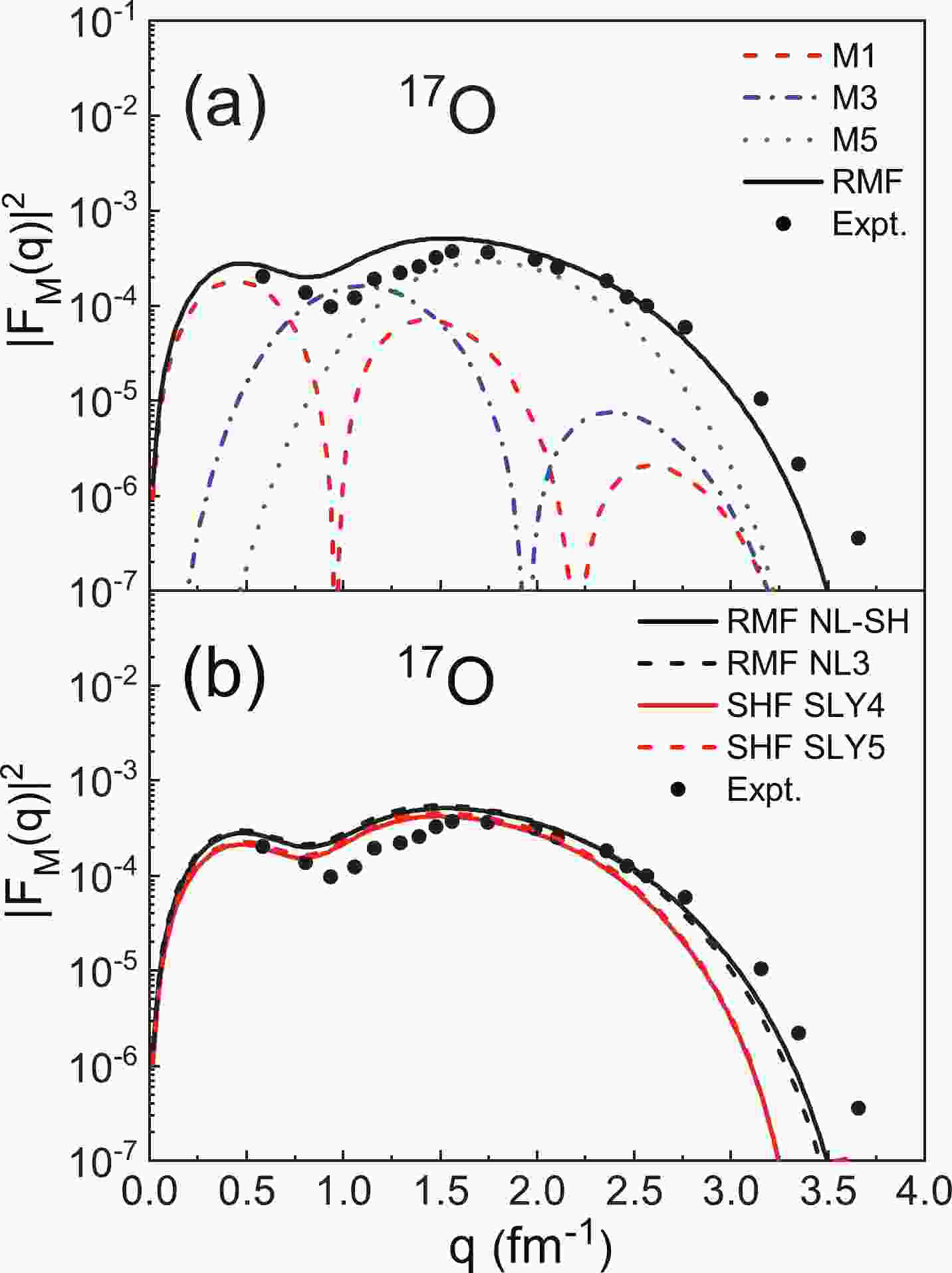
$ ^{17} {\rm{O}}$ with$ I^ {\pi} = 5/2^ {+} $ . We use the RMF and SHF models to generate the single-particle wave functions of the last neutron with the parameters NL-SH, NL3, SLY4, and SLY5. The multipole components M1, M3, and M5 of the magnetic form factors are presented in Fig. 1(a). It can be seen that the first peak of the total form factors is mainly from the contributions of the M1 multipole. In the high-q region,$ |F_{\mathrm{M}}(q)|^{2} $ are largely determined by the M5 multipole, as the values of M1 and M3 rapidly decrease as q becomes larger. In Fig. 1(b), we present the comparison of$ |F_{\mathrm{M}}(q)|^{2} $ of$ ^{17} {\rm{O}}$ calculated using the RMF and SHF models, respectively. The experimental data are also included in this figure. It can be seen that the$ |F_{\mathrm{M}}(q)|^{2} $ calculated by the SHF model are smaller than that obtained with the RMF model overall. The theoretical results of these two models coincide with the experimental data in and medium q regions, but in the high-q region, the theoretical form factors still fall more deeply than the experimental data.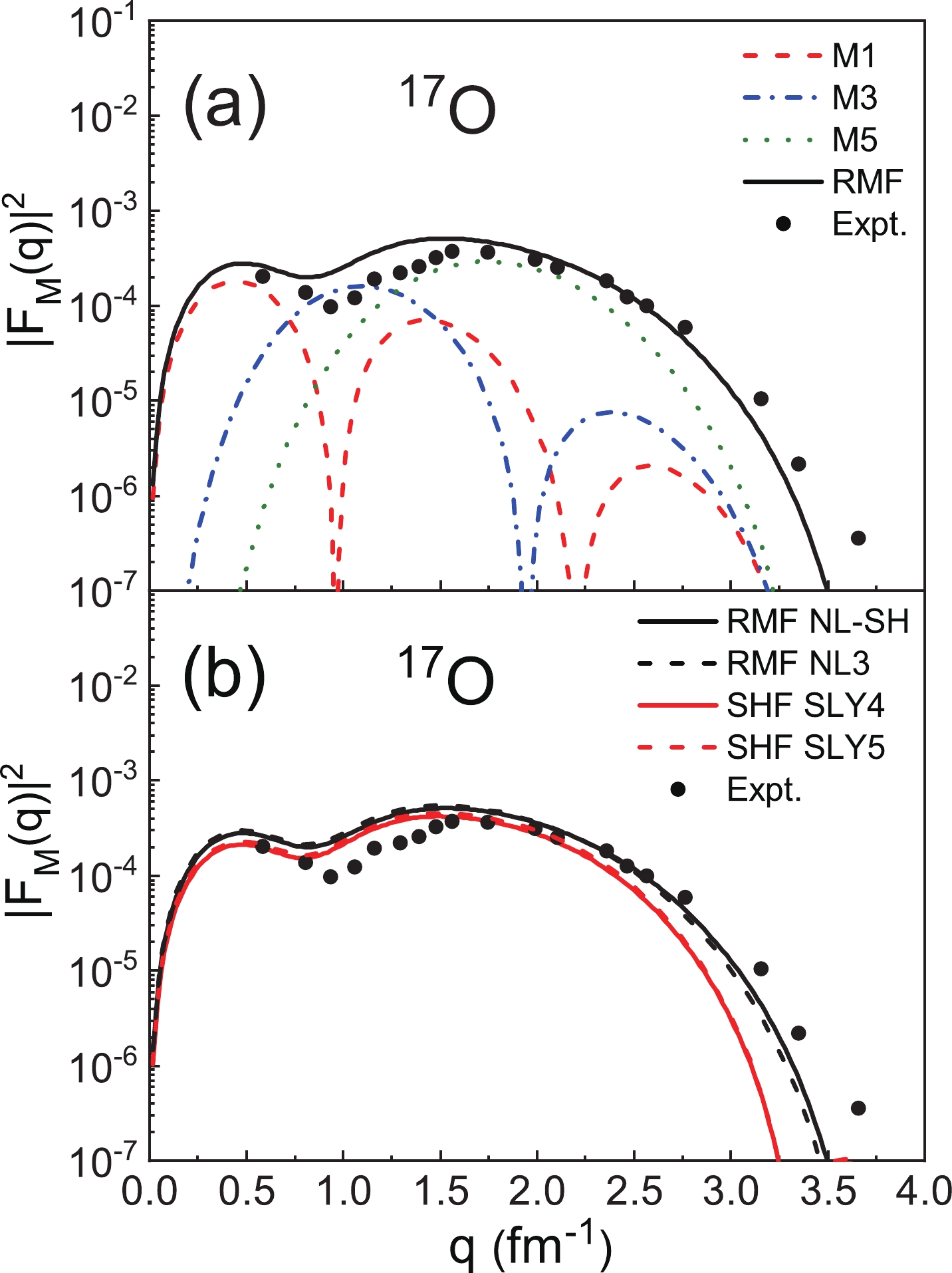
Figure 1. (color online) (a) The multipole components M1, M3, and M5 of the magnetic form factors of 17O (
$ I^ {\pi} = 5/2^ {+} $ ) obtained with the RMF model. (b) The magnetic form factors of 17O, where the wave functions are obtained from the RMF and SHF models. The experimental data are obtained from Ref. [23].There are many RMF and SHF parameter sets, and different parameter sets provide different theorical results. Therefore, we calculate
$ |F_{\mathrm{M}}(q)|^{2} $ from several parametrizations of the RMF and SHF models, and the comparison is also presented in Fig. 1(b). It can be seen that the NL-SH and NL3 [64] parameters lead to very close$ |F_{\mathrm{M}}(q)|^{2} $ , and similar results are obtained for the SLY4 and SLY5 [50] parameters. There are two groups of$ |F_{\mathrm{M}}(q)|^{2} $ calculated with different models, which means that the$ |F_{\mathrm{M}}(q)|^{2} $ values are insensitive to the parameters of the RMF and SHF models. The discrepancies in$ |F_{\mathrm{M}}(q)|^{2} $ are mainly caused by the different models rather than the parametrizations. Therefore, we only show the results from the NL-SH and SLY4 parameter sets in the following sections.In Fig. 1(b),
$ |F_{\mathrm{M}}(q)|^{2} $ calculated by the SHF model are smaller than those obtained with the RMF model. This is due to the different descriptions of the single-particle orbital in the RMF and SHF models. In the PWBA framework, the elastic magnetic form factors can be expressed by the Fourier transformation of the transition current density directly related to the density distribution of the valence nucleon. In Fig. 2 we further present the corresponding density distributions of the valence nucleon$ ^{17} {\rm{O}}$ , which occupies the$1d _{5/2} $ orbital. From Fig. 2, it can be seen that the density distributions from the RMF model are clearly larger than those from the SHF model in most regions except for the edge part. By performing the Fourier transformation from the coordinate space to the momentum space, the magnetic form factors calculated by the RMF model are larger than those of the SHF model, especially in the high-momentum transfers. This is because the form factor at large q is mainly determined by the valence nucleon density distribution at small coordinates in the r space. The differences between the RMF and SHF models in describing the single-particle orbital lead to differences in the magnetic form factors.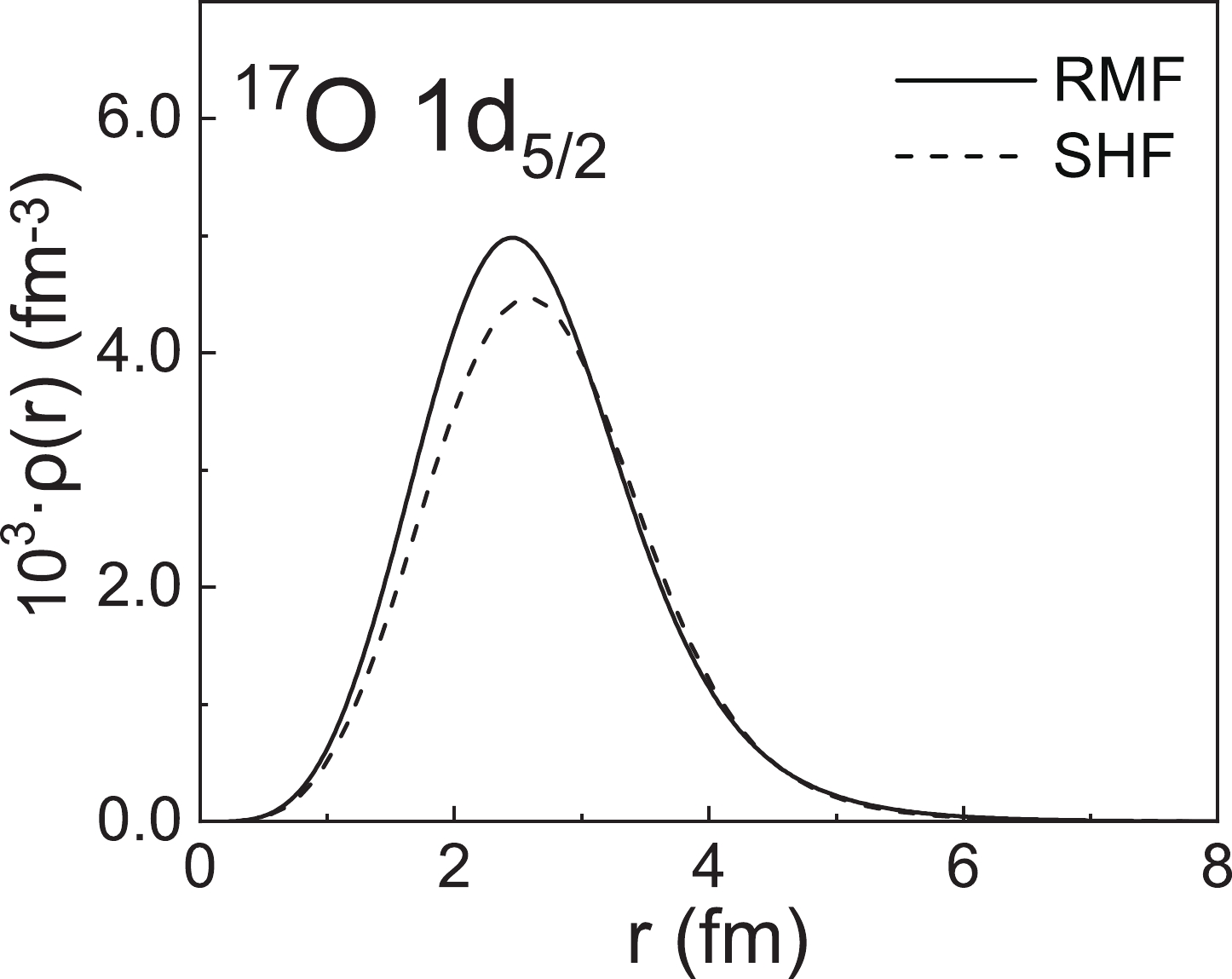
Figure 2. The density distribution of 17O when the valence nucleon occupies the
$ 1d_{5/2}$ orbital, where the single-particle wave functions are calculated using the RMF model with the NL-SH parameter set and SHF model with the SLY4 parameter set.The valence nucleon RMS radii
$ R_{\mathrm{V}} $ calculated from the RMF and SHF models are 3.399 and 3.409 fm, respectively. These results are consistent with the experimental data reported in Ref. [24] and the other theoretical results reported in Refs. [42, 65].Figure 3 shows the magnetic form factors of
$ ^{41} {\rm{Ca}}$ with$ I^ {\pi} = 7/2 ^ {-} $ , where the experimental data are taken from Ref. [22]. It can also be seen that the M1 multipole determines the first peak in Fig. 3(a). The values of M1, M3, and M5 decrease with increasing q. In the high-q region, the total form factors are mainly determined by the M7 multipole. In Fig. 3(b), it can be seen that the differences in$ |F_{\mathrm{M}}(q)|^{2} $ are still mainly in the high-momentum transfer. To illustrate this problem, we also display the valence nucleon density distributions of$ ^{41} {\rm{Ca}}$ in Fig. 4. Similar to Fig. 2, the density distributions at small coordinates in the$ r $ space lead to differences in the form factors at large coordinates in the p space, which indicates that the RMF and SHF models provide different descriptions of the single-particle orbital.
Figure 3. (color online) (a) The multipole components M1, M3, M5, and M7 of the magnetic form factors of 41Ca (
$ I^ {\pi} = 7/2^ {-} $ ) obtained with the RMF model. (b) The magnetic form factors of 41Ca, where the wave functions are obtained from the RMF and SHF models. The experimental data are obtained from Ref. [22].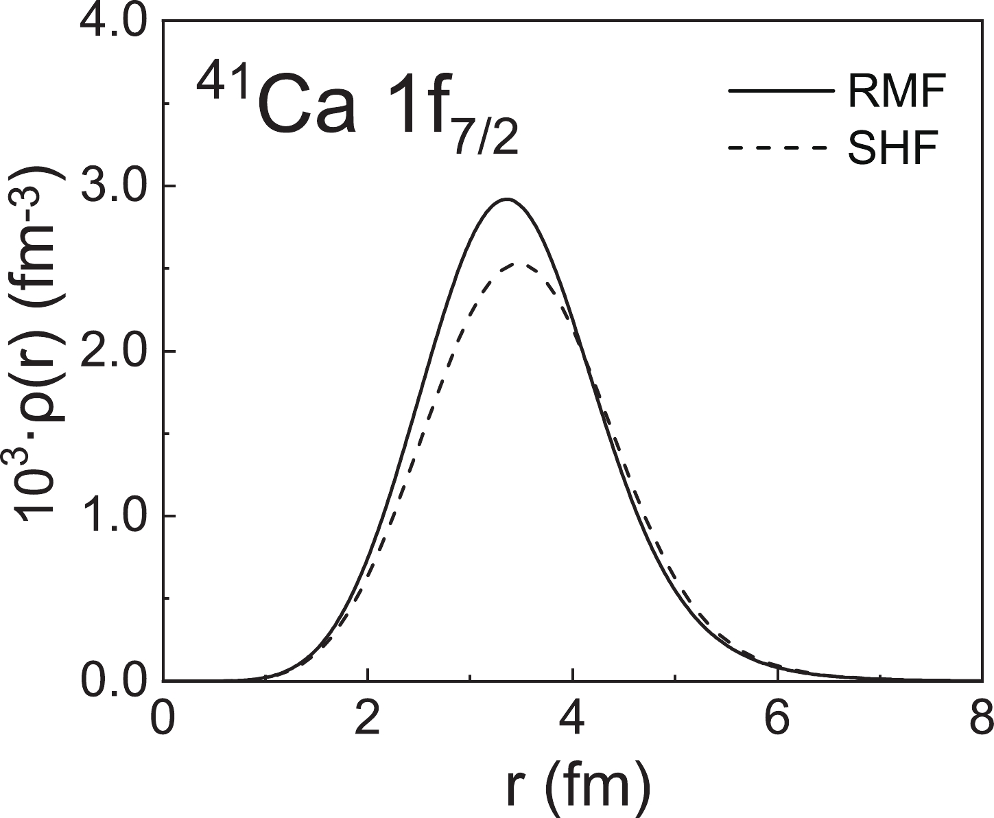
Figure 4. The density distributions of 41Ca when the valence nucleon occupies the
$ 1f_{_{7/2}}$ orbital, where the single-particle wave functions are calculated using the RMF model with the NL-SH parameter set and SHF model with the SLY4 parameter set.The valence nucleon RMS radii
$ R_{\mathrm{V}} $ of the$ 1 f_{ 7/2} $ orbital obtained from the sub-Coulomb transfer reactions are 4.00$ \pm $ 0.06 fm [66] and 3.89$ \pm $ 0.12 fm [67]. We obtain$ R_{\mathrm V} = 3.996 $ fm from the RMF model and$ R_{\mathrm V} = 4.063 $ fm from the SHF model, which are similar to the experimental results. The agreement between the theoretical results and experimental data implies the validity of the RMF and SHF theories in reproducing the magnetic form factors.From the calculations of these two selected spherical nuclei, we found that the
$ |F_{\mathrm{M}}(q)|^{2} $ from the RMF and SHF models in Sec. II can quite reasonably reproduce the measured electromagnetic form factors well. Overall, the$ |F_{\mathrm{M}}(q)|^{2} $ obtained from the SHF model is slightly smaller than that obtained from the RMF model. In the low-q and middle-q regions, there are little differences between the results of the RMF and SHF models, while in the high-q region, more obvious differences can be seen. The origin of these differences can be traced back to the effective nuclear interaction. The self-consistent central potentials from the RMF model are deeper than those from the SHF model, which leads to different descriptions of the single-particle orbital from the RMF and SHF models. The RMF model provides larger single-particle orbital density distributions at the center and peak region, so the magnetic form factors related to density from the RMF model are also larger than those from the SHF model, especially in the high-q region. -
In this section, we investigate the
$ |F_{\mathrm{M}}(q)|^{2} $ of deformed nuclei$ ^{11} {\rm{B}}$ ,$ ^{27} {\rm{Al}}$ ,$ ^{59} {\rm{Co}}$ , and$ ^{115} {\rm{In}}$ based on the deformed scattering formulas Eqs. (20) - (26) in Sec. II. The theoretical$ |F_{\mathrm{M}}(q)|^{2} $ for the selected nuclei are calculated from the relativistic RMF and non-relativistic SHF models. A comparison of the results reflects the differences in describing the properties of single-particle by the RMF and SHF models.In Fig. 5, we present the results of
$ ^{11} {\rm{B}}$ with$ I^ {\pi} = 3/2 ^ {-} $ . Figure 5(a) and Fig. 5(b) show$ |F_{\mathrm{M}}(q)|^{2} $ from both the spherical and deformed calculations with the RMF model. M1 and M3 in the spherical descriptions are relatively large overall, which leads to the final result being larger than the experimental data. For the nucleus$ ^{11} {\rm{B}}$ with the valence nucleon in the$ 1p_{ 3/2} $ state, we should note that the geometric factors$ {\eta}^{L = 1}_{3/2} $ and$ {\eta}^{L = 3}_{3/2} $ are both equal to 0.6 using Eq. (25). Therefore, in the deformed case, the overall contributions of the M1 and M3 multipoles decrease due to geometric factors. Figure 5(c) shows a comparison between the results of the SHF and RMF models. After taking the deformation into account, the results of the two models become smaller, which are more consistent with the experimental data. However, there are also some differences between them. In the high-q region, it can be seen that$ |F_{\mathrm{M}}(q)|^{2} $ calculated with the SHF model are smaller than those of the RMF model, which reflects the differences in the wave functions between the two models.
Figure 5. (color online) (a) The magnetic form factors of 11B (
$ I^ {\pi} = 3/2^ {-} $ ) divided into the M1 and M3 multipole components in the spherical RMF model. (b) The multipole components in the deformed case. (c) A comparison between$ |F_{\mathrm{M}}(q)|^{2} $ from the RMF and SHF calculations. The experimental data are obtained from [23].Figure 6 shows the same results, but for
$ ^{27} {\rm{Al}}$ with$ I^ {\pi} = 5/2 ^ {+} $ . In Fig. 6(a) of the spherical case, all the multipoles come into play. In the region$ q < 1 \;{\rm{fm}} ^{-1} $ , the first peak is mainly determined by the M1 multipole. The magnetic form factors are filled due to the contribution of the M3 multipole in the region between the two peaks$ 1 < \;q\; < \;2 \;\mathrm{fm}^{-1} $ . In the high-q region, the M5 multipole plays a dominant role. For the deformed calculations shown in Fig. 6(b), it can be seen that the agreement between the theoretical results and the experimental data is obviously improved, especially in the dip region$ 1 < \;q\; < \;1.5 \;\mathrm{fm}^{-1} $ , which is mainly determined by the M3 multipole. For the nucleus$ ^{27} {\rm{Al}}$ , the introduction of the geometric factor$ {\eta}^{L = 3}_{5/2} = 0.1190 $ reduces the contributions of M3, which can better describe the dip of the experimental data. In Fig. 6(c),$ |F_{\mathrm{M}}(q)|^{2} $ calculated with the deformation calculations based on the RMF and SHF models are compared, and both are consistent with the experimental data. However, the results of the two models are also different in that the RMF model results are larger than those of the SHF model overall, especially in the high-momentum transfers region. According to Eq. (16), the differences in the wave functions are amplified with the increase of L, and therefore a more obvious difference in the magnetic form factors is observed in the high-momentum transfer region.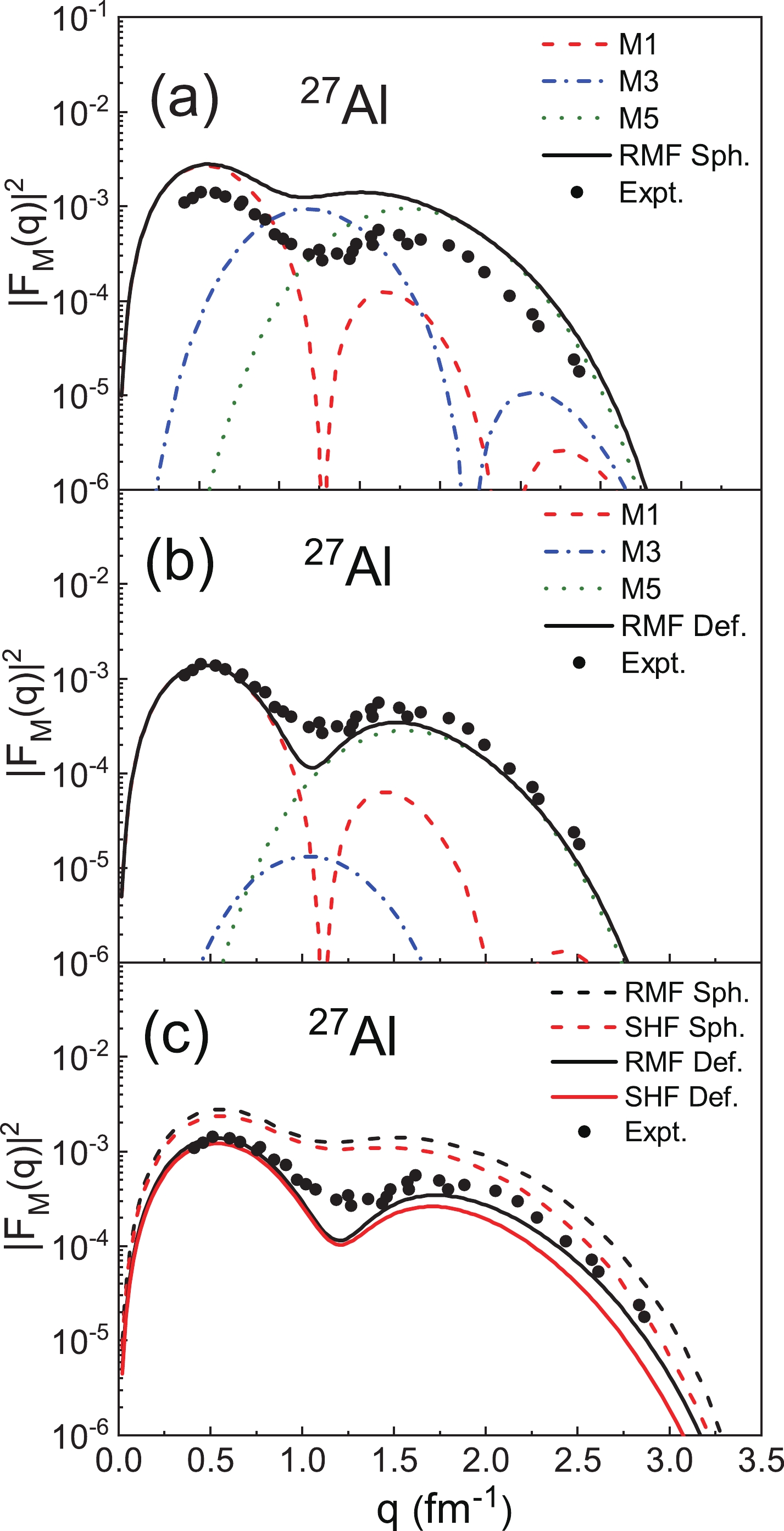
Figure 7 shows the results for
$ ^{59} {\rm{Co}}$ with$ I^ {\pi} = 7/2 ^ {-} $ . Again, in Fig. 7(a) of the spherical case, M1, M3, M5, and M7 all contribute to the total form factors, and the overall theoretical results are above the experimental data. In Fig. 7(b) of the deformed case, due to the geometrical factors$ {\eta}^{L = 3}_{7/2} = 0.2121 $ and$ {\eta}^{L = 5}_{7/2} = 0.0163 $ , the contributions of the M3 and M5 multipoles are greatly reduced, which gives a better description of the downward trend of the experimental data in the region$ 0.5 < \;q\; < \;1 \;\mathrm{fm}^{-1} $ . In Fig. 7(c), we present$ |F_{\mathrm{M}}(q)|^{2} $ calculated using the RMF and SHF models, and it can be seen that the results of both the models are in good agreement with the experimental data. The differences in$ |F_{\mathrm{M}}(q)|^{2} $ between the RMF and SHF models are small in the low-q region but become more obvious in the middle-q and high-q regions. However, the results of the RMF model are still overall larger than those of the SHF model, which can be attributed to the different descriptions of the single-particle orbital between the two models.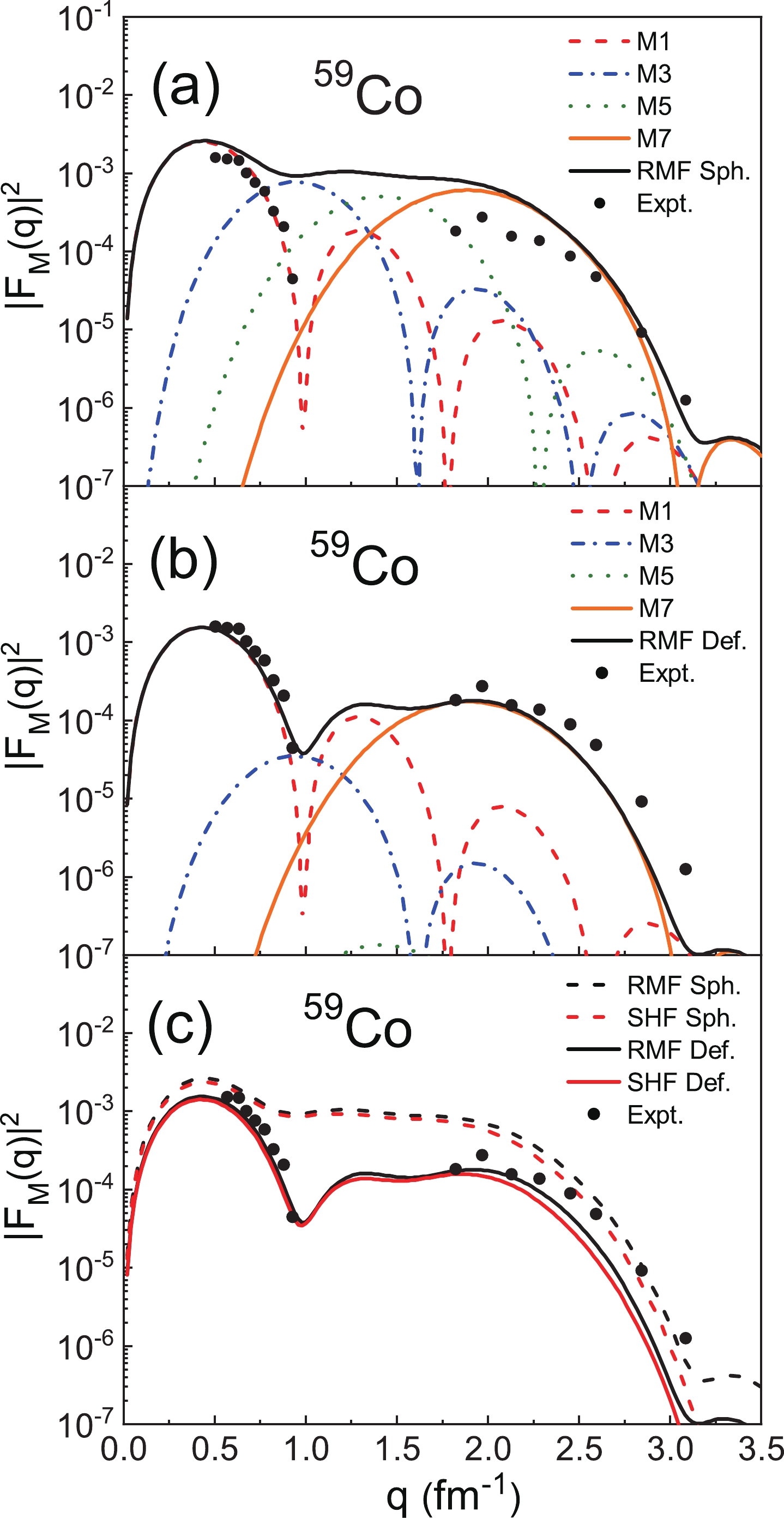
Finally, Fig. 8 shows the results for
$ ^{115} {\rm{In}}$ with$ I^ {\pi} = 9/2 ^ {+} $ . In Fig. 8(a) of the spherical calculations, every multipole plays a role, and the curve of the magnetic form factors is relatively flat with no obvious peak value. M3 and M5 fill the magnetic form factors in the region$ 0.5 < \;q\; < \;1 \;\mathrm{fm}^{-1} $ . In Fig. 8(b) of the deformed case, the geometrical factors$ {\eta}^{L = 3}_{9/2} = 0.2397 $ ,$ {\eta}^{L = 5}_{9/2} = 0.0419 $ , and$ {\eta}^{L = 7}_{9/2} = 0.0019 $ , which greatly reduces the contribution of M3, M5, and M7 to the total form factors. The deformed case reproduces the results of three peaks. The M1 multipole determines the two first peaks, while the third peak is due to the M9 multipole. The roles of M5 and M7 are negligible owing to the geometrical factors. In Fig. 8(c), it can be seen that$ |F_{\mathrm{M}}(q)|^{2} $ in the deformed case show better agreement with the experimental data. For the deformed nucleus$ ^{115} {\rm{In}}$ , the differences in the wave functions calculated with the two models are small, so the differences in$ |F_{\mathrm{M}}(q)|^{2} $ are not obvious in the entire q region.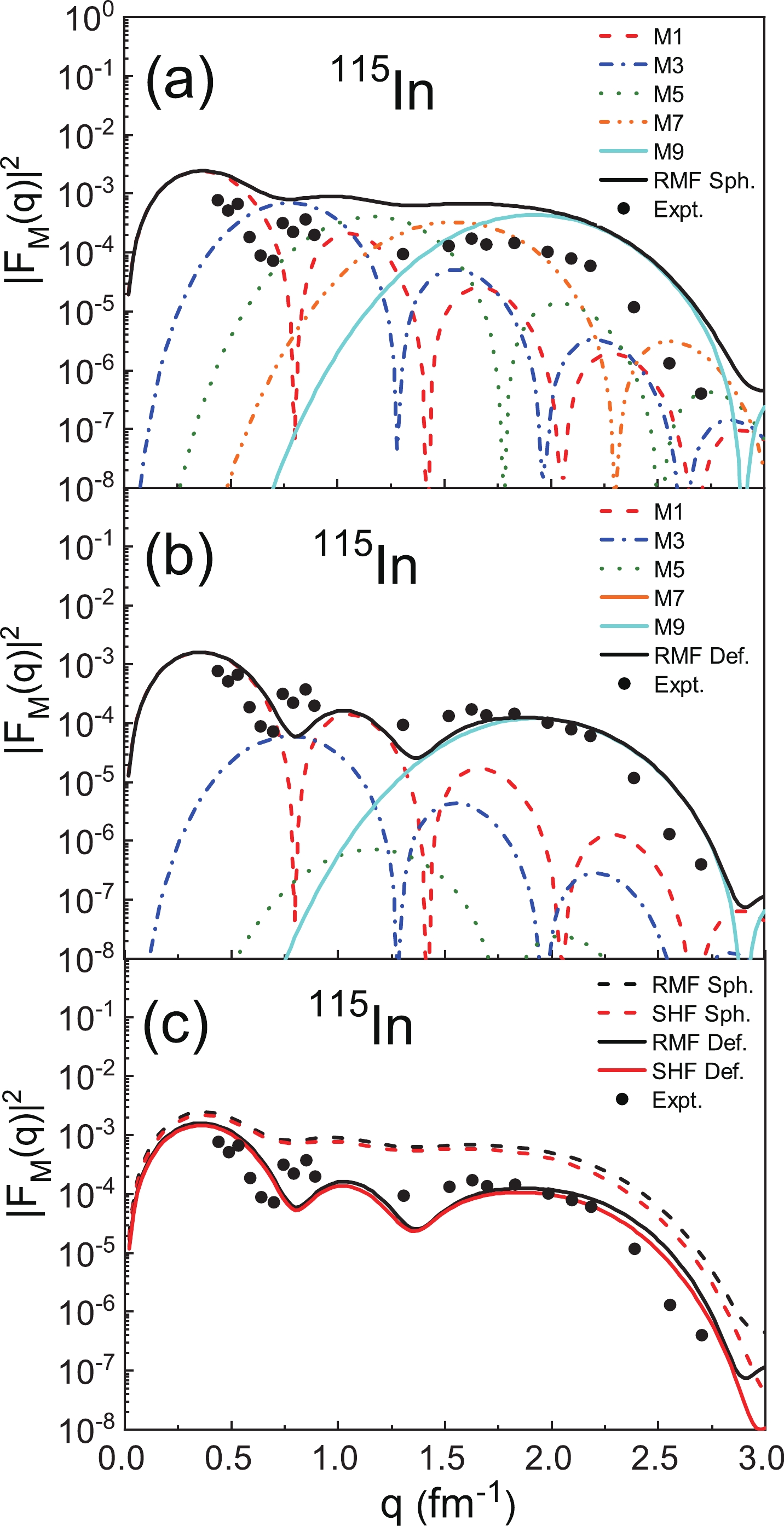
In summary, it can be found that with the addition of geometrical factors, the multipoles of the deformed form decrease with respect to the spherical ones, which also helps to improve the consistency of the deformed case with the experimental data. The corrections introduced by deformation have a positive effect on the description of deformed nuclei.
In the studies presented in Sec. III.A and III.B, the RMF and SHF models are constructed without considering the pairing interaction. There are various ways to incorporate the effects of pairing, such as the BCS or Bogolybov transformations. It should be mentioned that the pairing interaction has a slight effect on the valence nucleon wave functions, but does not change the orbital of the valence nucleon. Therefore, the influence of the pairing interaction on
$ |F_{\mathrm{M}}(q)|^{2} $ is small and can be ignored. -
In this part, based on the models constructed in Sec. II, the magnetic form factors
$ |F_{\mathrm{M}}(q)|^{2} $ of exotic nuclei are studied to understand the structure of exotic nuclei. Assuming a valence nucleon in different orbitals with the same angular momentum, the corresponding$ |F_{\mathrm{M}}(q)|^{2} $ are calculated to reveal the relation between$ R_{\mathrm{V}} $ and$ |F_{\mathrm{M}}(q)|^{2} $ . Besides,$ |F_{\mathrm{M}}(q)|^{2} $ from the RMF and SHF models are also investigated and compared to show the different descriptions of the single-particle oribitals in an exotic region from different effective interactions.In Fig. 9, we first display the valence nucleon density distributions and corresponding
$ R_{\mathrm{V}} $ of$ ^{57} {\rm{Ti}}$ for different orbitals with the same angular momentum. It is clear that there are distinct differences between the density distributions of different orbitals. In general, the single-particle wave functions and valence nucleon density distributions are related to the node number. In Fig. 9, there is one peak for the valence nucleon density distribution of the$1 p_{3/2} $ orbital, but two peaks for those of the$2 p_{3/2} $ orbital. With an increase in the node number, the valence nucleon RMS radius in the$ 2 p_{3/2} $ orbital is considerably larger than that in$1 p_{3/2} $ .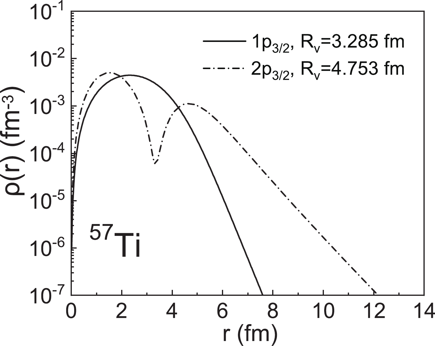
Figure 9. The valence nucleon density distributions of the
$ 1p_{3/2}$ orbital and$ 2p_{3/2}$ orbital for 57Ti, where the single-particle wave functions are calculated using the RMF model with the NL-SH parameter.In previous studies, the relation between
$ |F_{\mathrm{M}}(q)|^{2} $ and different angular momenta of the valence nucleon has been discussed [32]. We further calculate$ |F_{\mathrm{M}}(q)|^{2} $ where two valence nucleons have the same angular momentum but different valence nucleon RMS radii. In this way, the relation between$ R_{\mathrm{V}} $ and$ |F_{\mathrm{M}}(q)|^{2} $ can be reflected. In Fig. 10, we present$ |F_{\mathrm{M}}(q)|^{2} $ of$ ^{57} {\rm{Ti}}$ for different orbitals with the same angular momentum. It can be seen that with an increase in$ R_{\mathrm{V}} $ , the multipole components decrease more slowly, which leads to an extension of the total magnetic form factor. Due to the same angular momentum in Fig. 10(a) and Fig. 10(b), the differences in the total form factor are solely due to the transition current density, which is directly related to the valence nucleon RMS radii.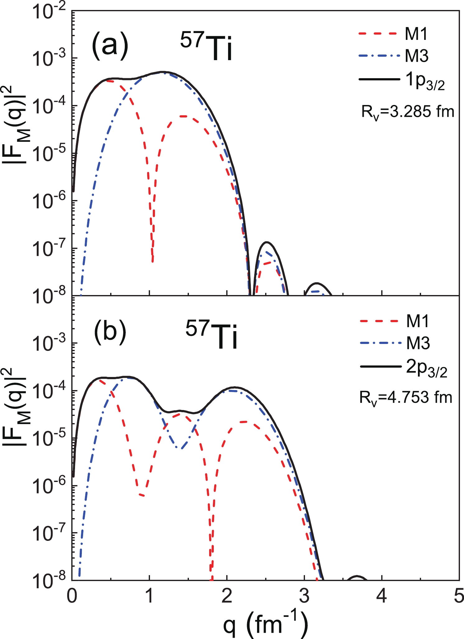
Figure 10. (color online) The magnetic form factors of the
$ 1p_{3/2}$ orbital and$ 2p_{3/2}$ orbital for 57Ti, where the single particle wave functions are calculated using the RMF model with the NL-SH parameter.Different effective interactions may provide different descriptions in the exotic region. It is also interesting to compare the magnetic form factors from different interactions for the exotic nuclei. In recent years, the first electron scattering experiment of
$ ^{132} {\rm{Xe}}$ has been successfully completed at a self-confining radioactive-isotope ion target (SCRIT) facility [68]. The ultimate purpose of this experiment is to complete the electron scattering experiment of the double magic nucleus$ ^{132} {\rm{Sn}}$ [69]. It can be foreseen that the magnetic electron scattering of$ ^{132} {\rm{Sn}}$ will be performed in the near future. Therefore, we chose$ ^{133} {\rm{Sn}}$ as the target nucleus to analyze the differences in the theoretical magnetic form factor between the RMF and SHF models.In Fig. 11 we plot the density distributions of
$ ^{133} {\rm{Sn}}$ where the valence nucleon occupies the$1 h_{9/2} $ orbital. Due to the relativistic effects, there are notable discrepancies in the central potentials and single-particle wave functions for these two models [37]. Based on the single-particle wave functions obtained from the RMF and SHF models, we show in Fig. 12 the magnetic form factors of$ ^{133} {\rm{Sn}}$ calculated in the relativistic and non-relativistic frameworks, respectively. It can be seen that the differences in$ |F_{\mathrm{M}}(q)|^{2} $ mainly occur in the high-momentum transfer region. The magnetic form factors at large coordinates in the p space mainly depend on the current density at the small coordinates of the r space. The differences in$ |F_{\mathrm{M}}(q)|^{2} $ in the high-q region indicate that the single-particle wave functions generated by the RMF and SHF models are different in the low r region. These results can provide useful guidance for the electron scattering experiments of exotic nuclei in the future.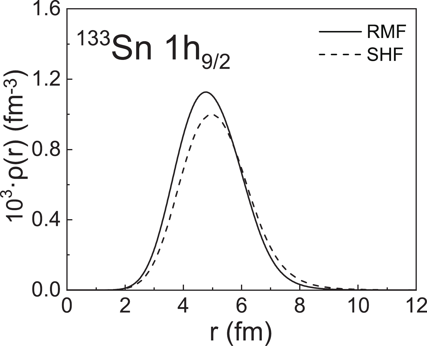
Figure 11. The density distributions of 133Sn when the last neutron occupies the
$ 1h_{9/2}$ orbital, where the single-particle wave functions are calculated using the RMF model with the NL-SH parameter and SHF model with the SLY4 parameter.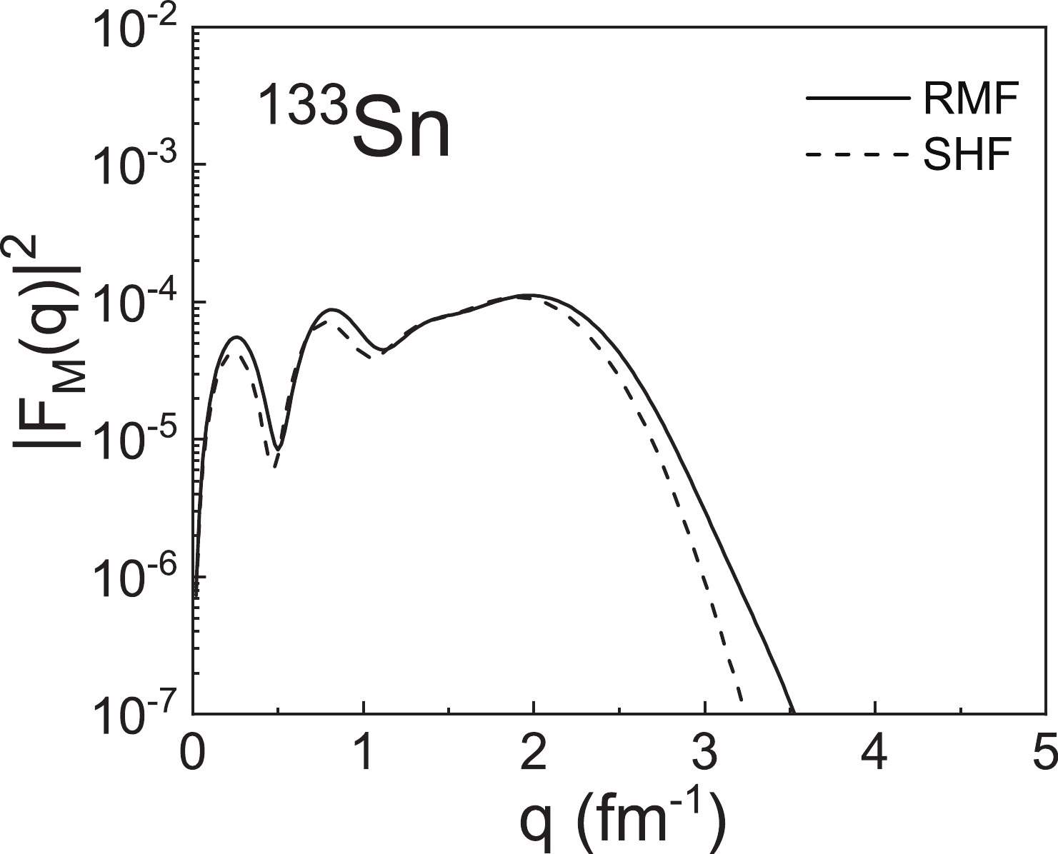
Figure 12. The magnetic form factors of 133Sn when the last neutron occupies the
$ 1h_{9/2}$ orbital, where the single-particle wave functions are calculated using the RMF model with the NL-SH parameter and SHF model with the SLY4 parameter. -
In this study, the magnetic form factors
$ |F_{\mathrm{M}}(q)|^{2} $ of spherical and deformed cases were investigated systematically using the RMF and SHF models. The magnetic form factor is significant for investigating the magnetic properties of nuclei. In previous studies, the RMF and SHF models were used to calculate the$ |F_{\mathrm{M}}(q)|^{2} $ under spherical symmetry. In this work, we further considered the deformation of the nuclei and conducted comparative studies of the magnetic form factors calculated using the RMF and SHF models, which reflect the differences in the description of the single-particle orbital between the two models.This research is divided into three parts. First, the single-particle wave functions are obtained with the RMF and SHF models. Second, the theoretical frameworks of non-relativistic and relativistic magnetic electron scattering are constructed, and the spherical limit method is used to calculate
$ |F_\mathrm{M}(q)|^{2} $ . Third, for the spherical cases, we calculate the$ |F_\mathrm{M}(q)|^{2} $ of spherical nuclei ($ ^{17} {\rm{O}}$ and$ ^{41} {\rm{Ca}}$ ) based on the RMF and SHF models. The spherical results of these two models coincide with the experimental data. For the deformed nuclei ($ ^{11} {\rm{B}}$ ,$ ^{17} {\rm{Al}}$ ,$ ^{59} {\rm{Co}}$ , and$ ^{115} {\rm{In}}$ ), there are some differences between the$ |F_{\mathrm{M}}(q)|^{2} $ values obtained with the two spherical models and the experimental data, especially at the middle-momentum transfer. Considering the influences of deformation on$ |F_{\mathrm{M}}(q)|^{2} $ , geometrical factors are introduced to modify the spherical results, and a clear improvement in the agreement between the theoretical results and experimental data is observed. To understand the structure of the exotic region, the magnetic form factors$ |F_{\mathrm{M}}(q)|^{2} $ of exotic nuclei are also studied.Different from the charge form factors that reflect the contributions of all the nucleus, the magnetic form factors
$ |F_{\mathrm{M}}(q)|^{2} $ for odd-A nuclei mainly reflect the properties of the valence nucleon. These results show the reliability of the single-particle wave functions generated by the two models. The$ |F_{\mathrm{M}}(q)|^{2} $ values obtained using the SHF model are smaller than those obtained with the RMF model, especially in the high-momentum transfers, which reflects the differences in the descriptions of the wave functions of the valence nucleons between the two models. The obvious discrepancies between the two models that occur in the high-momentum transfer are caused by the angular momentum-dependent term in the scattering matrix elements, which amplifies the differences between the wave functions derived using the two models. Due to the relativistic effects, the self-consistent central potentials from the RMF model are deeper than those from the SHF model, which leads to different single-particle orbital descriptions from the RMF and SHF models. The results of this study can be used to test the validity of models and can serve as a useful guide for the investigation of exotic nuclei.
Comparative studies on nuclear elastic magnetic form factors between the relativistic and non-relativistic mean-field approaches
- Received Date: 2021-06-30
- Available Online: 2022-01-15
Abstract: It is known that elastic magnetic electron scattering can be used to study the magnetic properties of nuclei and determine the outermost-shell single-particle orbitals. In this study, the magnetic form factors


 DownLoad: