


 Abstract
 HTML
HTML Reference
 Related
 PDF
PDF


-
Besides the conventional mesons and baryons, which are composed of a quark-antiquark pair and three quarks, there exist hadrons composed of more than three quarks or gluons. These states are called exotic states, such as a tetraquark [1, 2], pentaquark [3, 4], molecule [5-7], glueball [8, 9], and hybrid [10, 11]. In 2003, the first charmonium like state,
$ X(3872) $ , was observed by the Belle Collaboration in the exclusive$ B^{\pm}{\rightarrow}K^{\pm}\pi^{+}\pi^{-}J/\psi $ decays [12]. Its quantum number is$ I^{G}J^{PC} = 0^{+}1^{++} $ [13]. The discovery of$ X(3872) $ opened a new era of hadron spectroscopy. Since then, many charmonium like and bottomonium like states have been found, such as the$ Y(4260) $ [14],$ Z_{c}(3900) $ [15, 16],$ Z_{b}(10610) $ , and$ Z_{b}(10650) $ [17] states. In the fully heavy sector, the LHCb collaboration observed a narrow structure and a wide structure in the$ J/\psi $ -pair invariant mass spectrum in the range of$ 6.2\sim7.2\; \text{GeV} $ , which could be all-charm hadrons [18]. More details can be found in Refs. [19-26] and the references therein.The heavy quarks in these states are in hidden flavor(s). In 2017, the LHCb Collaboration observed
$ \Xi_{cc}^{++} $ in the$ \Lambda_c^+K^-\pi^+\pi^+ $ decay channel [27]. Its mass was determined to be$3621.40\pm0.72(\text{stat.}) \pm0.27(\text{syst.}) \pm 0.14(\Lambda_c^+)$ MeV. This is the first doubly heavy baryon observed in experiments. The$ \Xi_{cc}^{++} $ baryon gives implications for doubly heavy tetraquarks [28, 29], which are exotic states with open heavy flavors. Recently, the LHCb Collaboration observed a very narrow state in the$ D^{0}D^{0}\pi^{+} $ mass spectrum [30-33]. Under the$ J^{P} = 1^{+} $ assumption, its mass with respect to$ D^{*+}D^{0} $ and width are$ \delta{m}_{\text{BW}} = -273\pm61\pm5_{-14}^{+11}\; \text{keV}\,, $

(1) and
$ \Gamma_{\text{BW}} = 410\pm165\pm43_{-38}^{+18}\; \text{keV}\,, $

(2) respectively. The statistic significance of the signal is over
$ 10\sigma $ , whereas that for$ \delta{m}_{\text{BW}}<0 $ is$ 4.3\sigma $ . This structure is consistent with the$ DD^{*} $ molecule interpretation predicted by Li et al. within the one-boson-exchange (OBE) model [34]. The discovery of$ T_{cc}^{+} $ inspired many related studies [35-44]. Actually, doubly heavy tetraquarks have been studied extensively, with models such as the quark model [1, 45-72], QCD sum rules [73-83], lattice QCD [84-102], OBE potentials [34, 103-107], and chiral perturbation theory [108-111]. Their production has also been studied (for instance, see Refs. [112, 113]). The studies suggest that the masses of some of the doubly heavy tetraquarks are lighter than the thresholds of two mesons, which makes them stable against strong and electromagnetic decays. For example, Du et al. [76] studied$ QQ\bar{q}\bar{q}' $ ($ Q = c,b $ and$ q,q' = u,d,s $ ) in the QCD sum rules. They found that the$ bb\bar{q}\bar{q}' $ 's are stable. The stableness of doubly heavy tetraquarks is also supported by lattice QCD calculations. Leskovec et al. [100] used lattice QCD to investigate the spectrum of a$ \bar{b}\bar{b}ud $ four-quark system with quantum numbers$ I(J^{P}) = 0(1^+) $ , and obtained a binding energy of$ (-128\pm24\pm10)\; \text{MeV} $ , corresponding to the mass,$ 10476\pm24\pm10\; \text{MeV} $ . Mohanta and Basak [102] studied$ bb\bar{u}\bar{d} $ states on a lattice using a non relativistic QCD (NRQCD) action for a bottom and highly improved staggered quark (HISQ) action for light up/down quarks. They obtained the binding energy for the$ 1^{+} $ $ bb\bar{u}\bar{d} $ tetraquark system to be$ -189(18)\; \text{MeV} $ compared to$ BB^{*} $ . Using the$ \Xi_{cc}^{++} $ mass as the input, Karliner and Rosner [29] predicted the mass of the ground state of the$ IJ^{P} = 01^{+} $ doubly charm tetraquark ($ T_{cc} $ ) to be$ 3882.2\pm12\; \text{MeV} $ in a chromomagnetic model.In the quark model [114-118], the mass of a hadron can be decomposed into the quark masses, kinetic energy and potentials, which include the color-independent Coulomb and confinement interactions, and hyperfine interactions like spin-spin, spin-orbit, and tensor terms. If we restrict to the S-wave states, the spin-orbit and tensor interactions do not contribute. We can use an extended chromomagnetic model [1, 58, 118-127]. In this model, the masses of S-wave hadrons consist of effective quark masses, color interaction, and chromomagnetic interaction. This simplified model provides good account of all S-wave mesons and baryons [125]. In this work, we use an extended chromomagnetic model to study S-wave doubly heavy tetraquarks. With the obtained wave function, we further use a simple method to estimate the partial decay ratios of the tetraquark states. In Sec. II we introduce the methods of the present work, The numerical results are presented and discussed in Sec. III. We conclude the study in Sec. IV.
-
In a chromomagnetic model, the Hamiltonian of an S-wave hadron is [123, 125-131]
$ H = \sum\limits_{i}m_{i}+H_{\text{CE}}+H_{\text{CM}}, $

(3) where
$ m_i $ is the effective mass of the ith quark,$ H_{\text{CE}} $ is the chromoelectric (CE) interaction [123, 125-127], where$ H_{\text{CE}} = - \sum\limits_{i<j} a_{ij} {\boldsymbol{F}}_{i}\cdot{\boldsymbol{F}}_{j}\,, $

(4) and
$ H_{\text{CM}} $ is the chromomagnetic (CM) interaction [1, 26, 120-122], where$ H_{\text{CM}} = - \sum\limits_{i<j} v_{ij} {\boldsymbol{S}}_{i}\cdot{\boldsymbol{S}}_{j} {\boldsymbol{F}}_{i}\cdot{\boldsymbol{F}}_{j}\,. $

(5) Here,
$ a_{ij} $ and$ v_{ij}\propto\left\langle {\alpha_{s}(r_{ij})\delta({\bf{r}}_{ij})} \right\rangle/m_{i}m_{j} $ are effective coupling constants that depend on the constituent quark masses and the spatial wave function.$ {\boldsymbol{S}}_{i} = {\boldsymbol{\sigma}}_i/2 $ and$ {\boldsymbol{F}}_{i} = {\boldsymbol{\lambda}}_i/2 $ are the quark spin and color operators. For an antiquark,$ {\boldsymbol{S}}_{\bar{q}} = -{\boldsymbol{S}}_{q}^{*}\,, \quad {\boldsymbol{F}}_{\bar{q}} = -{\boldsymbol{F}}_{q}^{*}\,. $

(6) Since
$ \begin{aligned} \sum\limits_{i<j} \left(m_i+m_j\right) {\boldsymbol{F}}_{i}\cdot{\boldsymbol{F}}_{j} = {} \left(\sum\limits_{i}m_{i}{\boldsymbol{F}}_i\right) \cdot \left(\sum\limits_{i}{\boldsymbol{F}}_{i}\right) - \frac{4}{3} \sum\limits_{i} m_{i}\,, \end{aligned} $

(7) and the total color operator,
$ \sum_i{\boldsymbol{F}}_i $ , nullifies any color-singlet physical state, we can rewrite the Hamiltonian as [125-127]$ H = -\frac{3}{4} \sum\limits_{i<j}m_{ij}V^{\text{C}}_{ij} - \sum\limits_{i<j}v_{ij}V^{\text{CM}}_{ij} \,, $

(8) where
$ m_{ij} = \left(m_i+m_j\right) + \frac{4}{3} a_{ij}\,, $

(9) is the quark pair mass parameter.
$ V^{\text{C}}_{ij} = {\boldsymbol{F}}_{i}\cdot{\boldsymbol{F}}_{j} $ and$ V^{\text{CM}}_{ij} = {\boldsymbol{S}}_{i}\cdot{\boldsymbol{S}}_{j}{\boldsymbol{F}}_{i}\cdot{\boldsymbol{F}}_{j} $ are the color and CM interactions between quarks. -
To investigate the masses of tetraquarks, we need to construct wave functions. The total wave function is a direct product of the orbital, color, spin, and flavor wave functions. Here, the orbital wave function is symmetric because we only consider the S-wave states. Because the Hamiltonian does not contain a flavor operator explicitly, we first construct the color-spin wave function, and then incorporate the flavor wave function to account for the Pauli principle.
The spins of tetraquarks can be 0, 1, and 2. In the
$ qq{\otimes}\bar{q}\bar{q} $ configuration, the possible color-spin wave functions,$ \{\alpha_{i}^{J}\} $ , are listed as follows:1.
$ J^{P} = 0^{+} $ :$ \begin{aligned}[b] \alpha_{1}^{0} =& \left| {\left(q_1q_2\right)_{1}^{6}\left(\bar{q}_{3}\bar{q}_{4}\right)_{1}^{\bar{6}}} \right\rangle _{0}, \quad \alpha_{2}^{0} = \left| {\left(q_1q_2\right)_{0}^{6}\left(\bar{q}_{3}\bar{q}_{4}\right)_{0}^{\bar{6}}} \right\rangle _{0}, \\ \alpha_{3}^{0} =& \left| {\left(q_1q_2\right)_{1}^{\bar{3}}\left(\bar{q}_{3}\bar{q}_{4}\right)_{1}^{3}} \right\rangle _{0}, \quad \alpha_{4}^{0} = \left| {\left(q_1q_2\right)_{0}^{\bar{3}}\left(\bar{q}_{3}\bar{q}_{4}\right)_{0}^{3}} \right\rangle _{0}, \end{aligned}$

(10) 2.
$ J^{P} = 1^{+} $ :$ \begin{aligned}[b] \alpha_{1}^{1} =& \left| {\left(q_1q_2\right)_{1}^{6}\left(\bar{q}_{3}\bar{q}_{4}\right)_{1}^{\bar{6}}} \right\rangle _{1}, \quad \alpha_{2}^{1} = \left| {\left(q_1q_2\right)_{1}^{6}\left(\bar{q}_{3}\bar{q}_{4}\right)_{0}^{\bar{6}}} \right\rangle _{1}, \\ \alpha_{3}^{1} =& \left| {\left(q_1q_2\right)_{0}^{6}\left(\bar{q}_{3}\bar{q}_{4}\right)_{1}^{\bar{6}}} \right\rangle _{1}, \quad \alpha_{4}^{1} = \left| {\left(q_1q_2\right)_{1}^{\bar{3}}\left(\bar{q}_{3}\bar{q}_{4}\right)_{1}^{3}} \right\rangle _{1}, \\ \alpha_{5}^{1} =& \left| {\left(q_1q_2\right)_{1}^{\bar{3}}\left(\bar{q}_{3}\bar{q}_{4}\right)_{0}^{3}} \right\rangle _{1}, \quad \alpha_{6}^{1} = \left| {\left(q_1q_2\right)_{0}^{\bar{3}}\left(\bar{q}_{3}\bar{q}_{4}\right)_{1}^{3}} \right\rangle _{1}, \end{aligned}$

(11) 3.
$ J^{P} = 2^{+} $ :$ \begin{aligned}[b] \alpha_{1}^{2} = \left| {\left(q_1q_2\right)_{1}^{6}\left(\bar{q}_{3}\bar{q}_{4}\right)_{1}^{\bar{6}}} \right\rangle _{2}, \quad \alpha_{2}^{2} = \left| {\left(q_1q_2\right)_{1}^{\bar{3}}\left(\bar{q}_{3}\bar{q}_{4}\right)_{1}^{3}} \right\rangle _{2}, \end{aligned} $

(12) where superscript
$ 3 $ ,$ \bar{3} $ ,$ 6 $ , or$ \bar{6} $ denotes the color, and subscript 0, 1, or 2 denotes the spin.Next we consider the flavor wave function. There are six types of total wave functions when we consider the Pauli principle:
1. Type A:
$ \varphi_{\text{A}} = \{(nn\bar{Q}\bar{Q})^{I = 1},ss\bar{Q}\bar{Q}\} $ (a)
$ J^{P} = 0^{+} $ :$ \begin{array}{l} \Psi_{\text{A1}}^{0^+} = \varphi_{\text{A}}\otimes\alpha^{0}_{2}, \quad \Psi_{\text{A2}}^{0^+} = \varphi_{\text{A}}\otimes\alpha^{0}_{3}, \end{array} $

(13) (b)
$ J^{P} = 1^{+} $ :$ \Psi_{\text{A}}^{1^+} = \varphi_{\text{A}}\otimes\alpha^{1}_{4}, $

(14) (c)
$ J^{P} = 2^{+} $ :$ \Psi_{\text{A}}^{2^+} = \varphi_{\text{A}}\otimes\alpha^{2}_{2}, $

(15) 2. Type B:
$ \varphi_{\text{B}} = \{(nn\bar{Q}\bar{Q})^{I = 0}\} $ (a)
$ J^{P} = 1^{+} $ :$ \begin{array}{l} \Psi_{\text{B1}}^{1^+} = \varphi_{\text{B}}\otimes\alpha^{1}_{2}, \quad \Psi_{\text{B2}}^{1^+} = \varphi_{\text{B}}\otimes\alpha^{1}_{6}, \end{array} $

(16) 3. Type C:
$ \varphi_{\text{C}} = \{(nn\bar{c}\bar{b})^{I = 1},ss\bar{c}\bar{b}\} $ (a)
$ J^{P} = 0^{+} $ :$ \begin{array}{l} \Psi_{\text{C1}}^{0^+} = \varphi_{\text{C}}\otimes\alpha^{0}_{2}, \quad \Psi_{\text{C2}}^{0^+} = \varphi_{\text{C}}\otimes\alpha^{0}_{3}, \end{array}$

(17) (b)
$ J^{P} = 1^{+} $ :$ \begin{array}{l} \Psi_{\text{C1}}^{1^+} = \varphi_{\text{C}}\otimes\alpha^{1}_{3},\quad \Psi_{\text{C2}}^{1^+} = \varphi_{\text{C}}\otimes\alpha^{1}_{4}, \quad \Psi_{\text{C3}}^{1^+} = \varphi_{\text{C}}\otimes\alpha^{1}_{5}, \end{array}$

(18) (c)
$ J^{P} = 2^{+} $ :$ \Psi_{\text{C}}^{2^+} = \varphi_{\text{C}}\otimes\alpha^{2}_{2}, $

(19) 4. Type D:
$ \varphi_{\text{D}} = \{(nn\bar{c}\bar{b})^{I = 0}\} $ (a)
$ J^{P} = 0^{+} $ :$ \begin{array}{l} \Psi_{\text{D1}}^{0^+} = \varphi_{\text{D}}\otimes\alpha^{0}_{1},\quad \Psi_{\text{D2}}^{0^+} = \varphi_{\text{D}}\otimes\alpha^{0}_{4}, \end{array} $

(20) (b)
$ J^{P} = 1^{+} $ :$ \begin{array}{l} \Psi_{\text{D1}}^{1^+} = \varphi_{\text{D}}\otimes\alpha^{1}_{1}, \quad \Psi_{\text{D2}}^{1^+} = \varphi_{\text{D}}\otimes\alpha^{1}_{2}, \quad \Psi_{\text{D3}}^{1^+} = \varphi_{\text{D}}\otimes\alpha^{1}_{6}, \end{array} $

(21) (c)
$ J^{P} = 2^{+} $ :$ \Psi_{\text{D}}^{2^+} = \varphi_{\text{D}}\otimes\alpha^{2}_{1}, $

(22) 5. Type E:
$ \varphi_{\text{E}} = \{ns\bar{Q}\bar{Q}\} $ (a)
$ J^{P} = 0^{+} $ :$ \begin{array}{l} \Psi_{\text{E1}}^{0^+} = \varphi_{\text{E}}\otimes\alpha^{0}_{2},\quad \Psi_{\text{E2}}^{0^+} = \varphi_{\text{E}}\otimes\alpha^{0}_{3}, \end{array} $

(23) (b)
$ J^{P} = 1^{+} $ :$ \begin{array}{l} \Psi_{\text{E1}}^{1^+} = \varphi_{\text{E}}\otimes\alpha^{1}_{2}, \quad \Psi_{\text{E2}}^{1^+} = \varphi_{\text{E}}\otimes\alpha^{1}_{4},\quad \Psi_{\text{E3}}^{1^+} = \varphi_{\text{E}}\otimes\alpha^{1}_{6}, \end{array}$

(24) (c)
$ J^{P} = 2^{+} $ :$ \Psi_{\text{E}}^{2^+} = \varphi_{\text{E}}\otimes\alpha^{2}_{2}, $

(25) 6. Type F:
$ \varphi_{\text{F}} = \{ns\bar{c}\bar{b}\} $ $ \Psi_{\text{F}i}^{J^+} = \varphi_{\text{F}}\otimes\alpha^{J}_{i}, $

(26) Diagonalizing the Hamiltonian [Eq. (8)] in these bases, we can obtain the masses and eigenvectors of doubly heavy tetraquarks.
-
Next we consider the strong decay properties of tetraquarks. There are various methods for studying tetraquark decays, such as the dimeson decay through the quark interchange model [132-135] and the dibaryon decay through the
$ ^{3}{P}_{0} $ model [136-139]. These models require the dynamical structures of hadrons, which is beyond the power of a CM model. Here we adopt a simple method to estimate the partial decay ratios of tetraquark states.In Sec. II.B, we have described the construction of a wave function in the
$ qq{\otimes}\bar{q}\bar{q} $ configuration, wherein the tetraquark states are superpositions of the bases. The tetraquark states can also be written as linear superpositions of the bases in the$ q\bar{q}{\otimes}q\bar{q} $ configuration (see Appendix A). Normally, the$ q\bar{q} $ component in a tetraquark can be either a color-singlet or a color-octet. The former one can easily dissociate into two S-wave mesons in a relative S wave, which are called “Okubo-Zweig-Iizuka- (OZI-) superallowed” decays. The recoupling coefficient provides the overlap between a tetraquark and a particular meson$ \times $ meson state. Then, we can determine the decay amplitude of that tetraquark into that particular meson$ \times $ meson channel. The latter one can only fall apart through a gluon exchange [120, 140]. In this work, we focus on the “OZI-superallowed” decays.For each decay mode, the branching fraction is proportional to the square of the coefficient,
$ c_i $ , of the corresponding component in the eigenvectors, and also depends on the phase space. For a two body decay through an L-wave, the partial decay width is [126, 141]$ \Gamma_{i} = \gamma_{i}\alpha\frac{k^{2L+1}}{m^{2L}}{\cdot}|c_i|^2, $

(27) where m is the mass of the initial state, k is the momentum of the final states in the rest frame of the initial state,
$ \alpha $ is the effective coupling constant, and$ \gamma_{i} $ is a quantity determined by the decay dynamics. Generally,$ \gamma_{i} $ is determined by the spatial wave functions of both the initial and final states, which are different for each decay process. In the quark model, the spatial wave functions of the pseudoscalar and vector mesons are the same. Thus, for each tetraquark, we have$ \gamma_{M_{1}M_{2}} = \gamma_{M_{1}M_{2}^{*}} = \gamma_{M_{1}^{*}M_{2}} = \gamma_{M_{1}^{*}M_{2}^{*}} $

(28) where
$ M_{i} $ and$ M_{i}^{*} $ are pseudoscalar and vector mesons, respectively. Then, we can estimate the partial decay width ratios of the tetraquark states. -
To calculate tetraquark masses, one needs to estimate parameters
$ \{m_{ij}^{t},v_{ij}^{t}\} $ . In Ref. [125], we used meson and baryon masses to extract parameters$ \{m_{q_{1}\bar{q}_{2}}^{m},v_{q_{1}\bar{q}_{2}}^{m}\} $ and$ \{m_{q_{1}q_{2}}^{b},v_{q_{1}q_{2}}^{b}\} $ . Baryon parameters$ \{m_{Q_{1}Q_{2}}^{b},v_{Q_{1}Q_{2}}^{b}\} $ between two heavy quarks cannot be fitted from baryons because of the lack of experimental data. For this reason, we adopted the following assumptions:$ {\delta}a_{q_{1}q_{2}}^{bm} {\equiv} a_{q_{1}q_{2}}^{b}-a_{q_{1}\bar{q}_{2}}^{m} {\approx} 0 $

(29) and
$ R_{q_{1}q_{2}}^{bm} {\equiv} v_{q_{1}q_{2}}^{b}/v_{q_{1}\bar{q}_{2}}^{m} = 2/3\pm0.30 $

(30) to estimate them from meson parameters
$ \{m_{Q_{1}\bar{Q}_{2}}^{m} $ ,$ v_{Q_{1}\bar{Q}_{2}}^{m}\} $ . The resulting parameters are listed in Table 1. Because the CM interaction strengths,$ v_{ij} $ 's, are inversely proportional to the quark masses, meson parameters$ \{v_{c\bar{c}},v_{c\bar{b}},v_{b\bar{b}}\} $ between heavy flavors are quite small. Thus, the large uncertainty of the ratio,$ R_{q_{1}q_{2}}^{bm} $ , does not have much effect on baryon parameters$ \{v_{cc},v_{cb},v_{bb}\} $ and the mass spectra of doubly heavy tetraquarks. As shown in Ref. [125], the introduction of the first assumption makes the difference,$ \delta{m}_{q_{1}q_{2}}^{bm}{\equiv}m_{q_{1}q_{2}}^{b}-m_{q_{1}\bar{q}_{2}}^{m} $ , separable over the two quarks as follows:Parameter $m_{n\bar{n}}^{m}$ 

$m_{n\bar{s}}^{m}$ 

$m_{s\bar{s}}^{m}$ 

$m_{n\bar{c}}^{m}$ 

$m_{s\bar{c}}^{m}$ 

$m_{c\bar{c}}^{m}$ 

$m_{n\bar{b}}^{m}$ 

$m_{s\bar{b}}^{m}$ 

$m_{c\bar{b}}^{m}$ 

$m_{b\bar{b}}^{m}$ 

Value $615.95$ 

$794.22$ 

$936.40$ 

$1973.22$ 

$2076.14$ 

$3068.53$ 

$5313.35$ 

$5403.25$ 

$6322.27$ 

$9444.97$ 

Parameter $v_{n\bar{n}}^{m}$ 

$v_{n\bar{s}}^{m}$ 

$v_{s\bar{s}}^{m}$ 

$v_{n\bar{c}}^{m}$ 

$v_{s\bar{c}}^{m}$ 

$v_{c\bar{c}}^{m}$ 

$v_{n\bar{b}}^{m}$ 

$v_{s\bar{b}}^{m}$ 

$v_{c\bar{b}}^{m}$ 

$v_{b\bar{b}}^{m}$ 

Value $477.92$ 

$298.57$ 

$249.18$ 

$106.01$ 

$107.87$ 

$85.12$ 

$33.89$ 

$36.43$ 

$47.18$ 

$45.98$ 

Parameter $m_{nn}^{b}$ 

$m_{ns}^{b}$ 

$m_{ss}^{b}$ 

$m_{nc}^{b}$ 

$m_{sc}^{b}$ 

$m_{cc}^{b}$ 

$m_{nb}^{b}$ 

$m_{sb}^{b}$ 

$m_{cb}^{b}$ 

$m_{b{b}}^{b}$ 

Value $724.85$ 

$906.65$ 

$1049.36$ 

$2079.96$ 

$2183.68$ 

$3171.51$ 

$5412.25$ 

$5494.80$ 

$6416.07$ 

$9529.57$ 

Parameter $v_{n{n}}^{b}$ 

$v_{n{s}}^{b}$ 

$v_{ss}^{b}$ 

$v_{n{c}}^{b}$ 

$v_{s{c}}^{b}$ 

$v_{c{c}}^{b}$ 

$v_{n{b}}^{b}$ 

$v_{s{b}}^{b}$ 

$v_{c{b}}^{b}$ 

$v_{b{b}}^{b}$ 

Value $305.34$ 

$212.75$ 

$195.30$ 

$62.81$ 

$70.63$ 

$56.75$ 

$19.92$ 

$8.47$ 

$31.45$ 

$30.65$ 

Table 1. Parameters of the
$q\bar{q}$ pairs for mesons and of the$qq$ pairs for baryons [125] (in units of$\text{MeV}$ ).$ \delta{m}_{q_{1}q_{2}}^{bm} {\approx} {\delta}{m}_{q_{1}}^{bm} + {\delta}{m}_{q_{2}}^{bm} , $

(31) where
$ {\delta}{m}_{q}^{bm}{\equiv}m_{q}^{b}-m_{q}^{m} $ is the difference of the effective quark mass extracted from the baryons and mesons. In this way, ten$ \delta{m}_{q_{1}q_{2}}^{bm} $ 's reduce to four$ {\delta}{m}_{q}^{bm} $ 's. Actually, such property can be achieved by a weaker assumption. Namely, we assume that the difference,$ a_{q_{1}q_{2}}^{b}-a_{q_{1}\bar{q}_{2}}^{m} $ , is separable over the two quarks as follows:$ a_{q_{1}q_{2}}^{b} - a_{q_{1}\bar{q}_{2}}^{m} {\approx} \delta{a}_{q_{1}}^{bm} + \delta{a}_{q_{2}}^{bm} . $

(32) Then, we have
$ \delta{m}_{q_{1}q_{2}}^{bm} {\approx} {\delta}\tilde{m}_{q_{1}}^{bm} + {\delta}\tilde{m}_{q_{2}}^{bm} , $

(33) where
$ {\delta}\tilde{m}_{q}^{bm} {\equiv} m_{q}^{b}-m_{q}^{m}+\frac{4}{3}\delta{a}_{q}^{bm} = \delta{m}_{q}^{bm}+\frac{4}{3}\delta{a}_{q}^{bm} , $

(34) which includes the quark mass difference and the differences between the color interactions. We again reduce ten
$ \delta{m}_{q_{1}q_{2}}^{bm} $ 's into four degrees of freedom. All results are unchanged except that we reinterpret the$ \delta{m}_{q}^{bm} $ of Ref. [125] as$ {\delta}\tilde{m}_{q}^{bm} $ (see Table 2 or Table 6 of Ref. [125]).$\delta\tilde{m}_{n}^{bm}$ 

$\delta\tilde{m}_{s}^{bm}$ 

$\delta\tilde{m}_{c}^{bm}$ 

$\delta\tilde{m}_{b}^{bm}$ 

Value $54.94$ 

$56.48$ 

$51.49$ 

$42.30$ 

Table 2. Values of the difference
${\delta}\tilde{m}_{q}^{bm}=m_{q}^{b}-m_{q}^{m}+\frac{4}{3}\delta{a}_{q}^{bm}$ [125] (in units of$\text{MeV}$ ).Now we consider tetraquarks. In Ref. [127], we used the following scheme to estimate the masses of fully heavy tetraquarks:
$ m_{q_{i}q_{j}}^{t} \approx m_{q_{i}q_{j}}^{b}\,, $

(35) $ m_{q_{i}\bar{q}_{j}}^{t} \approx m_{q_{i}\bar{q}_{j}}^{m}\,, $

(36) $ v_{q_{i}q_{j}}^{t} \approx v_{q_{i}q_{j}}^{b}\,, $

(37) $ v_{q_{i}\bar{q}_{j}}^{t} \approx v_{q_{i}\bar{q}_{j}}^{m}\,. $

(38) Within this scheme, we found that the ground states of the fully heavy tetraquarks are dominated by color-sextet configurations, which is consistent with dynamical calculations [142, 143]. Nonetheless, this scheme ignores the difference in the spatial configurations between these tetraquarks and normal hadrons, which will evidently cause large uncertainties [1, 143, 144]. To appreciate the uncertainty, we introduce three additional schemes for comparison (see Table 3). Scheme III (IV) differs from scheme I (II) by
$m_{q_{i}q_{j}}^{t}$ 

$m_{q_{i}\bar{q}_{j}}^{t}$ 

$v_{q_{i}q_{j}}^{t}$ 

$v_{q_{i}\bar{q}_{j}}^{t}$ 

Scheme I $m_{q_{i}q_{j}}^{b}$ 

$m_{q_{i}\bar{q}_{j}}^{m}$ 

$v_{q_{i}q_{j}}^{b}$ 

$v_{q_{i}\bar{q}_{j}}^{m}$ 

Scheme II $m_{q_{i}q_{j}}^{b}$ 

$m_{q_{i}{q}_{j}}^{b}$ 

$v_{q_{i}q_{j}}^{b}$ 

$v_{q_{i}\bar{q}_{j}}^{m}$ 

Scheme III $m_{q_{i}q_{j}}^{b}$ 

$m_{q_{i}\bar{q}_{j}}^{m}$ 

$v_{q_{i}q_{j}}^{b}$ 

$v_{q_{i}{q}_{j}}^{b}$ 

Scheme IV $m_{q_{i}q_{j}}^{b}$ 

$m_{q_{i}{q}_{j}}^{b}$ 

$v_{q_{i}q_{j}}^{b}$ 

$v_{q_{i}{q}_{j}}^{b}$ 

Table 3. Possible choices of tetraquark parameters.
$ v_{q_{i}\bar{q}_{j}}^{t} \approx v_{q_{i}\bar{q}_{j}}^{m} \quad \Longrightarrow \quad v_{q_{i}\bar{q}_{j}}^{t} \approx v_{q_{i}{q}_{j}}^{b}\,. $

(39) Owing to the smallness of
$ v_{qQ}^{b} $ and$ v_{q\bar{Q}}^{m} $ , the results of scheme I (II) are very similar to those of scheme III (IV). Thus, we will focus on scheme I and scheme II. -
Inserting the parameters into the Hamiltonian, we can determine tetraquark masses. The masses and eigenvectors of the
$ nn\bar{Q}\bar{Q} $ tetraquarks are listed in Table 4. Here, we assume that the${SU}(2)$ flavor symmetry is exact and denote u, d quarks collectively as n. In the following, we use$ T_{i}(nn\bar{Q}\bar{Q},m,I,J^{P}) $ to represent the$ nn\bar{Q}\bar{Q} $ tetraquarks, where subscript i denotes the particular scheme of the parameters. In Figs. 1-2, we plot the relative positions of the$ nn\bar{Q}\bar{Q} $ tetraquarks and their meson-meson thresholds.System $J^{P}$ 

Scheme I Scheme II Mass Eigenvector Mass Eigenvector $(nn\bar{c}\bar{c})^{I=1}$ 

$0^{+}$ 

$3833.2$ 

$\{0.515,0.857\}$ 

$3969.2$ 

$\{0.350,0.937\}$ 

$4127.4$ 

$\{0.857,-0.515\}$ 

$4364.9$ 

$\{0.937,-0.350\}$ 

$1^{+}$ 

$3946.4$ 

$\{1\}$ 

$4053.2$ 

$\{1\}$ 

$2^{+}$ 

$4017.1$ 

$\{1\}$ 

$4123.8$ 

$\{1\}$ 

$(nn\bar{c}\bar{c})^{I=0}$ 

$1^{+}$ 

$3749.8$ 

$\{0.354,-0.935\}$ 

$3868.7$ 

$\{0.212,-0.977\}$ 

$3976.1$ 

$\{0.935,0.354\}$ 

$4230.8$ 

$\{0.977,0.212\}$ 

$(nn\bar{b}\bar{b})^{I=1}$ 

$0^{+}$ 

$10468.8$ 

$\{0.123,0.992\}$ 

$10569.3$ 

$\{0.086,0.996\}$ 

$10808.9$ 

$\{0.992,-0.123\}$ 

$11054.6$ 

$\{0.996,-0.086\}$ 

$1^{+}$ 

$10485.3$ 

$\{1\}$ 

$10584.2$ 

$\{1\}$ 

$2^{+}$ 

$10507.9$ 

$\{1\}$ 

$10606.8$ 

$\{1\}$ 

$(nn\bar{b}\bar{b})^{I=0}$ 

$1^{+}$ 

$10291.6$ 

$\{0.058,-0.998\}$ 

$10390.9$ 

$\{0.043,-0.999\}$ 

$10703.4$ 

$\{0.998,0.058\}$ 

$10950.3$ 

$\{0.999,0.043\}$ 

$(nn\bar{c}\bar{b})^{I=1}$ 

$0^{+}$ 

$7189.5$ 

$\{0.366,0.931\}$ 

$7305.6$ 

$\{0.232,0.973\}$ 

$7440.9$ 

$\{0.931,-0.366\}$ 

$7684.7$ 

$\{0.973,-0.232\}$ 

$1^{+}$ 

$7211.0$ 

$\{-0.311,-0.648,0.696\}$ 

$7322.5$ 

$\{-0.180,-0.687,0.704\}$ 

$7264.2$ 

$\{-0.048,0.742,0.669\}$ 

$7367.3$ 

$\{-0.029,0.719,0.694\}$ 

$7417.0$ 

$\{0.949,-0.175,0.262\}$ 

$7665.1$ 

$\{0.983,-0.104,0.150\}$ 

$2^{+}$ 

$7293.2$ 

$\{1\}$ 

$7396.0$ 

$\{1\}$ 

$(nn\bar{c}\bar{b})^{I=0}$ 

$0^{+}$ 

$7003.4$ 

$\{0.440,0.898\}$ 

$7124.6$ 

$\{0.266,0.964\}$ 

$7220.3$ 

$\{0.898,-0.440\}$ 

$7459.0$ 

$\{0.964,-0.266\}$ 

$1^{+}$ 

$7046.2$ 

$\{0.228,-0.219,0.949\}$ 

$7158.0$ 

$\{0.122,-0.133,0.984\}$ 

$7232.9$ 

$\{0.899,-0.327,-0.292\}$ 

$7482.4$ 

$\{0.910,-0.381,-0.165\}$ 

$7329.3$ 

$\{-0.374,-0.919,-0.122\}$ 

$7584.9$ 

$\{-0.397,-0.915,-0.074\}$ 

$2^{+}$ 

$7353.2$ 

$\{1\}$ 

$7610.3$ 

$\{1\}$ 

Table 4. Masses and eigenvectors of the
$nn\bar{c}\bar{c}$ ,$nn\bar{b}\bar{b}$ , and$nn\bar{c}\bar{b}$ tetraquarks. All masses are in units of MeV.
Figure 1. (color online) Mass spectra of the
$I=0$ (solid) and$I=1$ (dashed)$nn\bar{c}\bar{c}$ and$nn\bar{b}\bar{b}$ tetraquark states in scheme I (black) and scheme II (blue). The dotted lines indicate various meson-meson thresholds. All masses are in units of MeV.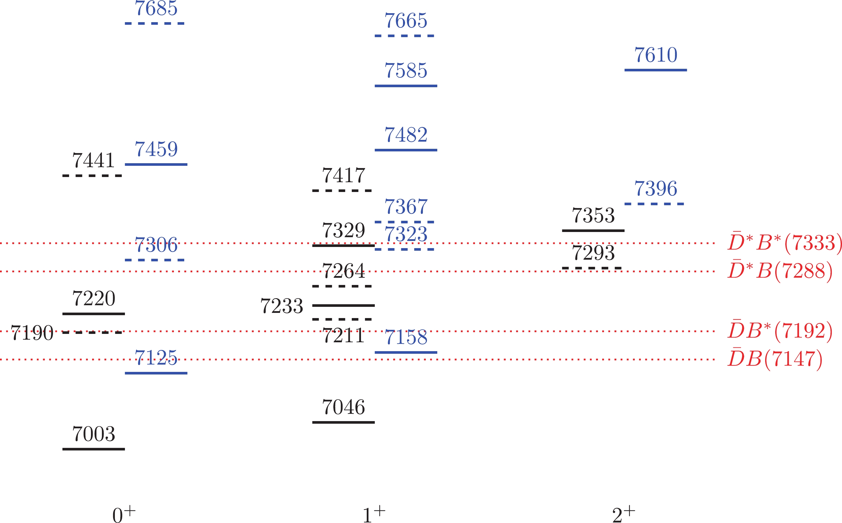
Figure 2. (color online) Mass spectra of the
$I=0$ (solid) and$I=1$ (dashed)$nn\bar{c}\bar{b}$ tetraquark states in scheme I (black) and scheme II (blue). The dotted lines indicate various meson-meson thresholds. All masses are in units of MeV.We first consider the
$ nn\bar{c}\bar{c} $ tetraquarks. The quantum number of their lightest state is$ IJ^{P} = 01^{+} $ , namely, the$ T_{I}(nn\bar{c}\bar{c},3749.8,0,1^{+}) $ or$ T_{II}(nn\bar{c}\bar{c},3868.7,0,1^{+}) $ state. The other isoscalar state is$ T_{I}(nn\bar{c}\bar{c},3976.1,0,1^{+}) $ or$ T_{II}(nn\bar{c}\bar{c},4230.8,0,1^{+}) $ . We find that scheme II always provides larger masses than scheme I. The reason is that the two schemes choose different values of$ m_{q_{i}\bar{q}_{j}}^{t} $ , which result in different values of the color interaction. More precisely, the difference in the color interactions between the two schemes is$ \begin{aligned}[b] \Delta{H}_{\text{C}} = & H_{\text{C}}^{II}-H_{\text{C}}^{I} = -\frac{3}{4}{\sum_\limits{i<j} } \left(m_{ij}^{II}-m_{ij}^{I}\right) V_{ij}^{\text{C}} \\=& -\frac{3}{4}{ \sum_\limits{i\leqslant 2}} {\sum_\limits{j>2} }\delta{m}_{ij}^{bm} V_{ij}^{\text{C}} \\ \approx & -\frac{3}{4} {\sum_\limits{i\leqslant 2} }{\sum_\limits{j>2}} \left(\delta\tilde{m}_{i}^{bm}+\delta\tilde{m}_{j}^{bm}\right) {\boldsymbol{F}}_{i}\cdot{\boldsymbol{F}}_{j} \\ =&\frac{3}{8} \left({ \sum_\limits{i}} \delta\tilde{m}_{i}^{bm} \right) \cdot \left( {\sum_\limits{i\leqslant 2}} {\boldsymbol{F}}_{i} \right)^{2} , \end{aligned}$

(40) where in the last line we ignore the terms proportional to
$ \sum_{i}{\boldsymbol{F}}_{i} $ . Note that both$ \left| {(q_{1}q_{2})^{6_{c}}(\bar{q}_{3}\bar{q}_{4})^{\bar{6}_{c}}} \right\rangle $ and$ \left| {(q_{1}q_{2})^{\bar{3}_{c}}(\bar{q}_{3}\bar{q}_{4})^{3_{c}}} \right\rangle $ are eigenstates of$ ({\boldsymbol{F}}_{1}+{\boldsymbol{F}}_{2})^{2} $ , with eigenvalues$ 10/3 $ and$ 4/3 $ , respectively. In other words,$ \left\langle {\Delta {H_{\rm{C}}}} \right\rangle = \left\{ \begin{array}{l} \dfrac{5}{4}\displaystyle\sum\limits_i \delta \tilde m_i^{bm}{\mkern 1mu} ,\;{\rm{for}}\;\left| {{{({q_1}{q_2})}^{{6_c}}}{{({{\bar q}_3}{{\bar q}_4})}^{{{\bar 6}_c}}}} \right\rangle ,\\ \dfrac{1}{2}\displaystyle\sum\limits_i \delta \tilde m_i^{bm}{\mkern 1mu} ,\;{\rm{for}}\;\left| {{{({q_1}{q_2})}^{{{\bar 3}_c}}}{{({{\bar q}_3}{{\bar q}_4})}^{{3_c}}}} \right\rangle {\mkern 1mu} . \end{array} \right. $

(41) For the
$ nn\bar{c}\bar{c} $ system,$ \sum_{i}\delta\tilde{m}_{i}^{bm} = 212.9\; \text{MeV} $ . The ground state,$ T_{I}(nn\bar{c}\bar{c},3749.8,0,1^{+}) $ , is dominated by the color-triplet configuration, and its mass is increased by about$ 118.9\; \text{MeV} $ . In contrast, the mass of the color-sextet configuration dominated state,$ T_{I}(nn\bar{c}\bar{c},3976.1,0,1^{+}) $ , is increased by$ 254.7\; \text{MeV} $ . The deviation from Eq. (41) is caused by the color mixing. In the isovector sector, we have four tetraquark states. They are all above the corresponding S-wave decay channels. It is interesting to note that the$ T_{II}(nn\bar{c}\bar{c},3686.7,0,1^{+}) $ state in scheme II is quite close to the newly observed$ T_{cc}^{+} $ state.The
$ nn\bar{b}\bar{b} $ tetraquarks are very similar to the$ nn\bar{c}\bar{c} $ tetraquarks. Their lightest state also has quantum number$ IJ^{P} = 01^{+} $ , namely, the$ T_{I}(nn\bar{b}\bar{b},10291.6,0,1^{+}) $ or$ T_{II}(nn\bar{b}\bar{b},10390.9,0,1^{+}) $ state. In both schemes, this state lies below the$ BB $ threshold and is stable against strong decays. In scheme I, the$ T_{I}(nn\bar{b}\bar{b},10468.9,1,0^{+}) $ ,$ T_{I}(nn\bar{b}\bar{b},10485.3,1,1^{+}) $ , and$ T_{I}(nn\bar{b}\bar{b},10507.9,1,2^{+}) $ states also lie below the the$ BB $ threshold. However, they are not stable in scheme II. Thus, we cannot draw a definite conclusion.Besides masses, eigenvectors also help understand the nature of tetraquarks. Within the four possible quantum numbers, the
$ IJ^{P} = 10^{+} $ one and the$ IJ^{P} = 01^{+} $ one are of particular interest because they both have two possible color configurations, namely, the color-sextet,$ \left| {(qq)^{6_{c}}{\otimes}(\bar{Q}\bar{Q})^{\bar{6}_{c}}} \right\rangle $ , and the color-triplet,$ \left| {(qq)^{\bar{3}_{c}}{\otimes}(\bar{Q}\bar{Q})^{{3}_{c}}} \right\rangle $ . For simplicity, we denote them as$ 6_{c}{\otimes}\bar{6}_{c} $ and$ \bar{3}_{c}{\otimes}{3}_{c} $ , respectively. As pointed out by Wang et al. [142], there are two competing effects in determining whether$ 6_{c}{\otimes}\bar{6}_{c} $ or$ \bar{3}_{c}{\otimes}{3}_{c} $ dominates the tetraquark ground state. In the one-gluon-exchange model, the color interactions in a color-triplet diquark are attractive, whereas those in a color-sextet diquark are repulsive. In contrast, both attractions between the$ 6_{c} $ diquark and the$ \bar{6}_{c} $ anti-diquark and between the$ \bar{3}_{c}{\otimes}{3}_{c} $ counterpart are attractive, and the former one is much stronger than the latter. The authors of Refs. [127, 142, 143] found that the color-sextet configuration has more net attraction for most fully heavy tetraquarks. Thus, the ground states contain more color-sextet components than the color-triplet ones. The only exception is the$ cc\bar{b}\bar{b} $ tetraquark in model II of Ref. [142], whose ground state has 53% of the$ \bar{3}_{c}{\otimes}3_{c} $ component. It is also interesting to note that, when the mass ratio between quarks and antiquarks deviates from one, the color-triplet configuration becomes more important in the ground states. For example, Ref. [127] found that$ T(bb\bar{b}\bar{b},18836.1,0^{++}) $ and$ T(cc\bar{c}\bar{c},6044.9,0^{++}) $ have 18.5% and 30.5% of the$ \bar{3}_{c}{\otimes}3_{c} $ components, respectively, whereas$ T(cc\bar{b}\bar{b},12596.3,0^{++}) $ has 48.4%. This tendency also exists in doubly heavy tetraquarks. As summarized in Table 4, the$ \bar{3}_{c}{\otimes}3_{c} $ components become dominant in the ground states of the$ nn\bar{Q}\bar{Q} $ tetraquarks. This phenomenon can also be explained by the color interaction Hamiltonian,$\begin{aligned}[b] &{\left\langle {{H_{\rm{C}}}\left( {nn\bar Q\bar Q} \right)} \right\rangle }\\ =&{ - \frac{3}{4}\left\langle {m_{nn}^tV_{12}^{\rm{C}} + m_{QQ}^tV_{34}^{\rm{C}} + m_{n\bar Q}^t\left( {V_{13}^{\rm{C}} + V_{24}^{\rm{C}} + V_{14}^{\rm{C}} + V_{23}^{\rm{C}}} \right)} \right\rangle }\\ =&{ - \frac{3}{4}\left\langle {m_{n\bar Q}^t\sum\limits_{i < j} {V_{ij}^{\rm{C}}} + 2\delta m\left( {V_{12}^{\rm{C}} + V_{34}^{\rm{C}}} \right)} \right\rangle }\\ =&{ 2m_{n\bar Q}^t - \frac{3}{2}\delta m\left\langle {V_{12}^{\rm{C}} + V_{34}^{\rm{C}}} \right\rangle }\\ =&{ 2m_{n\bar Q}^t + \delta m\left( {\begin{array}{*{20}{c}} { - 1}&0\\ 0&{ + 2} \end{array}} \right),} \end{aligned}$

(42) where we have expanded the Hamiltonian in the bases,
$\left\{ \left| {\left(n_1n_2\right)_{0}^{6}\left(\bar{Q}_{3}\bar{Q}_{4}\right)_{0}^{\bar{6}}} \right\rangle _{0} \right.$ ,$\left. \left| {\left(n_1n_2\right)_{1}^{\bar{3}}\left(\bar{Q}_{3}\bar{Q}_{4}\right)_{1}^{3}} \right\rangle _{0}\right\}$ , in the last line and$ \delta{m} = \frac{1}{2} \left(\frac{m_{nn}^{t}+m_{QQ}^{t}}{2}-m_{n\bar{Q}}^{t}\right). $

(43) Taking scheme I as an example, we have
$ \delta{m}\left(nn\bar{c}\bar{c}\right) = -12.52\; \text{MeV}\,, $

(44) $ \delta{m}\left(nn\bar{b}\bar{b}\right) = -93.07\; \text{MeV}\,, $

(45) whereas for the fully heavy tetraquarks,
$ \delta{m}\left(bb\bar{b}\bar{b}\right) = +42.30\; \text{MeV}\,, $

(46) $ \delta{m}\left(cc\bar{c}\bar{c}\right) = +51.49\; \text{MeV}\,, $

(47) $ \delta{m}\left(cc\bar{b}\bar{b}\right) = +15.15\; \text{MeV}\,. $

(48) As the ratio,
$ m_{\bar{q}}/m_{q} $ , increases, the$ \bar{3}_{c}{\otimes}3_{c} $ components become more important in the ground states.Another interesting conclusion from the Hamiltonian is that the color interaction does not mix the
$ 6_{c}{\otimes}\bar{6}_{c} $ and$ \bar{3}_{c}{\otimes}3_{c} $ configurations. Actually, this conclusion applies for all S-wave tetraquarks with$ q_{1} = q_{2} $ or$ \bar{q}_{3} = \bar{q}_{4} $ . Let us consider the matrix element of the color interaction,$ \left\langle {\alpha|H_{\text{CE}}|\beta} \right\rangle $ . Note that the color interaction is independent of the spin operator and thus is a rank-0 tensor in the$ q_{1}q_{2} $ spin space. Its matrix elements over different$ q_{1}q_{2} $ spin states always vanish. If$ q_{1} = q_{2} $ , the Pauli principle further renders the matrix elements to vanish, unless bases$ \alpha $ and$ \beta $ possess the same color symmetry over$ q_{1}q_{2} $ . The same argument applies to$ \bar{q}_{3}\bar{q}_{4} $ as well. In summary, the color interaction does no mix the$ 6_{c}{\otimes}\bar{6}_{c} $ and$ \bar{3}_{c}{\otimes}3_{c} $ color configurations if$ q_{1} = q_{2} $ or$ \bar{q}_{3} = \bar{q}_{4} $ .Next, we consider their decay properties. For the decays of the tetraquark states considered in this work, all
$ (k/m)^2 $ 's are of$ {\cal{O}}(10^{-2}) $ or even smaller order. All higher wave decays are suppressed. Thus, we only consider the S-wave decays in this work. First, we transform the wave functions of the$ nn\bar{Q}\bar{Q} $ tetraquarks into the$ n\bar{Q}{\otimes}n\bar{Q} $ configurations. Then, we can calculate the$ k\cdot|c_{i}|^2 $ 's and partial decay width ratios. The corresponding results are listed in Tables 5-10. Note that the two schemes obtain very similar results, and we mainly focus on scheme I in the following. In the isovector sector, the$ nn\bar{c}\bar{c} $ tetraquarks are mostly above the S-wave decay channel and thus have a wide state. Depending on the schemes, the$ J^{P} = 2^{+} $ state may lie on or above the$ \bar{D}^{*}\bar{D}^{*} $ threshold, namely the$ T_{I}(nn\bar{c}\bar{c},4017.1,1,2^{+}) $ or$ T_{II}(nn\bar{c}\bar{c},4123.8,1,2^{+}) $ state. A firm conclusion requires more detailed studies. The$ T_{I}(nn\bar{c}\bar{c},4127.4,1,0^{+}) $ state can decay into both$ \bar{D}\bar{D} $ and$ \bar{D}^{*}\bar{D}^{*} $ channels, with the partial decay width ratio,System $J^{P}$ 

Scheme I Scheme II Mass $\bar{D}^{*}\bar{D}^{*}$ 

$\bar{D}^{*}\bar{D}$ 

$\bar{D}\bar{D}^{*}$ 

$\bar{D}\bar{D}$ 

Mass $\bar{D}^{*}\bar{D}^{*}$ 

$\bar{D}^{*}\bar{D}$ 

$\bar{D}\bar{D}^{*}$ 

$\bar{D}\bar{D}$ 

$(nn\bar{c}\bar{c})^{I=1}$ 

$0^{+}$ 

$3833.2$ 

$0.116$ 

$0.639$ 

$3969.2$ 

$-0.023$ 

$0.611$ 

$4127.4$ 

$0.755$ 

$0.093$ 

$4364.9$ 

$0.763$ 

$0.207$ 

$1^{+}$ 

$3946.4$ 

$0$ 

$0.408$ 

$0.408$ 

$4053.2$ 

$0$ 

$0.408$ 

$0.408$ 

$2^{+}$ 

$4017.1$ 

$0.577$ 

$4123.8$ 

$0.577$ 

$(nn\bar{c}\bar{c})^{I=0}$ 

$1^{+}$ 

$3749.8$ 

$-0.177$ 

$0.415$ 

$-0.415$ 

$3868.7$ 

$-0.277$ 

$0.369$ 

$-0.369$ 

$3976.1$ 

$0.685$ 

$0.280$ 

$-0.280$ 

$4230.8$ 

$0.651$ 

$0.338$ 

$-0.338$ 

Table 5. Eigenvectors of the
$nn\bar{c}\bar{c}$ tetraquark states in the$n\bar{c}{\otimes}n\bar{c}$ configuration. All masses are in units of MeV.System $J^{P}$ 

Scheme I Scheme II Mass $\bar{D}^{*}\bar{D}^{*}$ 

$\bar{D}\bar{D}^{*}$ 

$\bar{D}\bar{D}$ 

Mass $\bar{D}^{*}\bar{D}^{*}$ 

$\bar{D}\bar{D}^{*}$ 

$\bar{D}\bar{D}$ 

$(nn\bar{c}\bar{c})^{I=1}$ 

$0^{+}$ 

$3833.2$ 

× $176.4$ 

$3969.2$ 

× $251.3$ 

$4127.4$ 

$270.0$ 

$7.6$ 

$4364.9$ 

$497.6$ 

$48.5$ 

$1^{+}$ 

$3946.4$ 

$61.9$ 

$4053.2$ 

$98.8$ 

$2^{+}$ 

$4017.1$ 

× $4123.8$ 

$155.3$ 

$(nn\bar{c}\bar{c})^{I=0}$ 

$1^{+}$ 

$3749.8$ 

× × $3868.7$ 

× × $3976.1$ 

× $34.7$ 

$4230.8$ 

$281.1$ 

$96.8$ 

Table 6. Values of
$k\cdot|c_{i}|^2$ for the$nn\bar{c}\bar{c}$ tetraquarks (in unit of MeV).System $J^{P}$ 

Scheme I Scheme II Mass $\bar{D}^{*}\bar{D}^{*}$ 

$\bar{D}\bar{D}^{*}$ 

$\bar{D}\bar{D}$ 

Mass $\bar{D}^{*}\bar{D}^{*}$ 

$\bar{D}\bar{D}^{*}$ 

$\bar{D}\bar{D}$ 

$(nn\bar{c}\bar{c})^{I=1}$ 

$0^{+}$ 

$3833.2$ 

× 1 $3969.2$ 

× 1 $4127.4$ 

$35.7$ 

1 $4364.9$ 

$10.3$ 

1 $1^{+}$ 

$3946.4$ 

1 $4053.2$ 

1 $2^{+}$ 

$4017.1$ 

× $4123.8$ 

1 $(nn\bar{c}\bar{c})^{I=0}$ 

$1^{+}$ 

$3749.8$ 

× × $3868.7$ 

× × $3976.1$ 

× 1 $4230.8$ 

$1.5$ 

1 Table 7. Partial width ratios for the
$nn\bar{c}\bar{c}$ tetraquarks. For each state, we choose one mode as the reference channel, and the partial width ratios of the other channels are calculated relative to this channel. All masses are in units of MeV.System $J^{P}$ 

Scheme I Scheme II Mass $B^{*}B^{*}$ 

$B^{*}B$ 

$BB^{*}$ 

$BB$ 

Mass $B^{*}B^{*}$ 

$B^{*}B$ 

$BB^{*}$ 

$BB$ 

$(nn\bar{b}\bar{b})^{I=1}$ 

$0^{+}$ 

$10468.8$ 

$-0.200$ 

$0.546$ 

$10569.3$ 

$-0.227$ 

$0.533$ 

$10808.9$ 

$0.737$ 

$0.344$ 

$11054.6$ 

$0.729$ 

$0.364$ 

$1^{+}$ 

$10485.3$ 

$0$ 

$0.408$ 

$0.408$ 

$10584.2$ 

$0$ 

$0.408$ 

$0.408$ 

$2^{+}$ 

$10507.9$ 

$0.577$ 

$10606.8$ 

$0.577$ 

$(nn\bar{b}\bar{b})^{I=0}$ 

$1^{+}$ 

$10291.6$ 

$-0.374$ 

$0.312$ 

$-0.312$ 

$10390.9$ 

$-0.383$ 

$0.306$ 

$-0.306$ 

$10703.4$ 

$0.600$ 

$0.391$ 

$-0.391$ 

$10950.3$ 

$0.594$ 

$0.395$ 

$-0.395$ 

Table 8. Eigenvectors of the
$nn\bar{b}\bar{b}$ tetraquark states in the$n\bar{b}{\otimes}n\bar{b}$ configuration. All masses are in units of MeV.System $J^{P}$ 

Scheme I Scheme II Mass $B^{*}B^{*}$ 

$BB^{*}$ 

$BB$ 

Mass $B^{*}B^{*}$ 

$BB^{*}$ 

$BB$ 

$(nn\bar{b}\bar{b})^{I=1}$ 

$0^{+}$ 

$10468.8$ 

× × $10569.3$ 

× $66.5$ 

$10808.9$ 

$503.0$ 

$136.5$ 

$11054.6$ 

$788.7$ 

$216.6$ 

$1^{+}$ 

$10485.3$ 

× $10584.2$ 

× $2^{+}$ 

$10507.9$ 

× $10606.8$ 

× $(nn\bar{b}\bar{b})^{I=0}$ 

$1^{+}$ 

$10291.6$ 

× × $10390.9$ 

× × $10703.4$ 

$193.6$ 

$111.0$ 

$10950.3$ 

$450.3$ 

$213.6$ 

Table 9. Values of
$k\cdot|c_{i}|^2$ for the$nn\bar{b}\bar{b}$ tetraquarks (in units of MeV).System $J^{P}$ 

Scheme I Scheme II Mass $B^{*}B^{*}$ 

$BB^{*}$ 

$BB$ 

Mass $B^{*}B^{*}$ 

$BB^{*}$ 

$BB$ 

$(nn\bar{b}\bar{b})^{I=1}$ 

$0^{+}$ 

$10468.8$ 

× × $10569.3$ 

× 1 $10808.9$ 

$3.7$ 

1 $11054.6$ 

$3.6$ 

1 $1^{+}$ 

$10485.3$ 

× $10584.2$ 

× $2^{+}$ 

$10507.9$ 

× $10606.8$ 

× $(nn\bar{b}\bar{b})^{I=0}$ 

$1^{+}$ 

$10291.6$ 

× × $10390.9$ 

× × $10703.4$ 

$0.9$ 

1 $10950.3$ 

$1.1$ 

1 Table 10. Partial width ratios for the
$nn\bar{b}\bar{b}$ tetraquarks. For each state, we choose one mode as the reference channel, and the partial width ratios of the other channels are calculated relative to this channel. All masses are in units of MeV.$ \Gamma_{\bar{D}^{*}\bar{D}^{*}}:\Gamma_{\bar{D}\bar{D}} \sim37.5\,. $

(49) Thus, the
$ \bar{D}^{*}\bar{D}^{*} $ mode is dominant. In the isoscalar sector, the$ T_{I}(nn\bar{c}\bar{c},3749.8,0,1^{+}) $ state lies below the$ \bar{D}\bar{D}^{*} $ threshold; thus, it is a narrow state. However, this state lies above the$ \bar{D}\bar{D} $ threshold; therefore, it can decay radiatively into the$ \bar{D}\bar{D}\gamma $ final states. The$ T_{I}(nn\bar{c}\bar{c}, 3976.1, $ $ 0,1^{+}) $ state is wide because it lies above the$ \bar{D}\bar{D}^{*} $ and$ \bar{D}^{*}\bar{D}^{*} $ thresholds. The$ T_{I}(nn\bar{b}\bar{b},10808.9,1,0^{+}) $ and$ T_{I}(nn\bar{b}\bar{b},10703.4,0,1^{+}) $ states lie above all corresponding S-wave decay channels. Their partial decay width ratios are$ \frac{\Gamma[T_{I}(nn\bar{b}\bar{b},10808.9,1,0^+){\rightarrow}B^{*}B^{*}]}{\Gamma[T_{I}(nn\bar{b}\bar{b},10808.9,1,0^+){\rightarrow}BB]} \sim3.7 $

(50) and
$ \frac{\Gamma[T_{I}(nn\bar{b}\bar{b},10703.4,0,1^+){\rightarrow}B^{*}B^{*}]}{\Gamma[T_{I}(nn\bar{b}\bar{b},10703.4,0,1^+){\rightarrow}BB]} \sim0.9 $

(51) respectively. All other
$ nn\bar{b}\bar{b} $ tetraquark states are narrow states. -
Next, we consider the
$ nn\bar{c}\bar{b} $ tetraquarks. We list the masses and eigenvectors of their states in Table 4. Their relative position and possible decay channels are plotted in Fig. 2. There are two possible stable$ nn\bar{c}\bar{b} $ tetraquark states. The first state is$ T_{I}(nn\bar{c}\bar{b},7003.4,0,0^{+}) $ , which lies below the$ \bar{D}B $ threshold by more than 100 MeV. Even in scheme II, this state is about 20 MeV below the threshold. The second state is$ T_{I}(nn\bar{c}\bar{b},7046.2,0,1^{+}) $ . It is about 100 MeV lighter than the$ \bar{D}B $ threshold. However, this state lies above the threshold in scheme II. Nonetheless, it lies below its S-wave decay mode$ \bar{D}B^{*} $ and thus should be a narrow state.Because the two antiquarks do not have to obey the Pauli principle, we have a much larger number of states than the
$ nn\bar{c}\bar{c} $ /$ nn\bar{b}\bar{b} $ cases. For each isospin, we have two$ 0^{+} $ states, three$ 1^{+} $ states, and one$ 2^{+} $ state. From Table 4, we see that for each possible quantum number, the lower mass states are dominated by the color-triplet configuration, whereas the color-sextet configuration is more important in the higher mass states. For example, the two stable states,$ T_{I}(nn\bar{c}\bar{b},7003.4,0,0^{+}) $ and$ T_{I}(nn\bar{c}\bar{b}, $ $ 7046.2,0,1^{+}) $ , have 80.6% and 90.0% of the$ \bar{3}_{c}{\otimes}3_{c} $ components, respectively. This can be explained by the color interaction,$ \left\langle {H_{\text{C}}\left(nn\bar{c}\bar{b}\right)} \right\rangle = m_{n\bar{c}} + m_{n\bar{b}} - \frac{3}{2} \delta{m}' \left\langle {V^{\text{C}}_{12}+V^{\text{C}}_{34}} \right\rangle, $

(52) where
$ \delta{m}' = {} \frac{1}{4} \left(m_{nn}+m_{cb}-m_{n\bar{c}}-m_{n\bar{b}}\right) = {} -36.41\; \text{MeV}. $

(53) Note that both the
$ 6_{c}\otimes\bar{6}_{c} $ and$ \bar{3}_{c}\otimes3_{c} $ configurations are eigenstates of$ V^{\text{C}}_{12}+V^{\text{C}}_{34} $ , with eigenvalues$ 2/3 $ and$ -4/3 $ , respectively. The negative value of$ \delta{m}' $ indicates that the color interaction favors the$ \bar{3}_{c}\otimes3_{c} $ configuration.In Table 11, we summarize the transformation of the
$ nn\bar{c}\bar{b} $ tetraquark states into the$ n\bar{c}{\otimes}n\bar{b} $ configuration. Then, we calculate the values of$ k\cdot|c_{i}|^2 $ and the relative partial decay widths, which are listed in Tables 12-13. Besides the two stable states discussed above, two heavier isoscalar states$ T_{I}(nn\bar{c}\bar{b},7220.3,0,0^{+}) $ and$ T_{I}(nn\bar{c}\bar{b},7232.9,0,1^{+}) $ are above the$ \bar{D}B^{*} $ mode, whereas the$ T_{I}(nn\bar{c}\bar{b},7329.3,0,1^{+}) $ state can decay into both$ \bar{D}^{*}B $ and$ \bar{D}B^{*} $ modes, with relative widthSystem $J^{P}$ 

Scheme I Scheme II Mass $\bar{D}^{*}B^{*}$ 

$\bar{D}^{*}B$ 

$\bar{D}B^{*}$ 

$\bar{D}B$ 

Mass $\bar{D}^{*}B^{*}$ 

$\bar{D}^{*}B$ 

$\bar{D}B^{*}$ 

$\bar{D}B$ 

$(nn\bar{c}\bar{b})^{I=1}$ 

$0^{+}$ 

$7189.5$ 

$-0.010$ 

$0.615$ 

$7305.6$ 

$-0.116$ 

$0.581$ 

$7440.9$ 

$0.764$ 

$0.197$ 

$7684.7$ 

$0.755$ 

$0.281$ 

$1^{+}$ 

$7211.0$ 

$0.104$ 

$0.063$ 

$-0.592$ 

$7322.5$ 

$0.184$ 

$-0.004$ 

$-0.557$ 

$7264.2$ 

$0.245$ 

$0.515$ 

$0.090$ 

$7367.3$ 

$0.266$ 

$0.506$ 

$0.081$ 

$7417.0$ 

$0.655$ 

$-0.383$ 

$0.241$ 

$7665.1$ 

$0.629$ 

$-0.401$ 

$0.316$ 

$2^{+}$ 

$7293.2$ 

$0.577$ 

$7396.0$ 

$0.577$ 

$(nn\bar{c}\bar{b})^{I=0}$ 

$0^{+}$ 

$7003.4$ 

$0.269$ 

$0.570$ 

$7124.6$ 

$0.374$ 

$0.466$ 

$7220.3$ 

$-0.587$ 

$0.508$ 

$7459.0$ 

$-0.526$ 

$0.605$ 

$1^{+}$ 

$7046.2$ 

$0.261$ 

$-0.231$ 

$0.495$ 

$7158.0$ 

$0.325$ 

$-0.268$ 

$0.409$ 

$7232.9$ 

$-0.308$ 

$0.469$ 

$0.568$ 

$7482.4$ 

$-0.287$ 

$0.417$ 

$0.633$ 

$7329.3$ 

$-0.580$ 

$-0.556$ 

$0.124$ 

$7584.9$ 

$-0.559$ 

$-0.581$ 

$0.123$ 

$2^{+}$ 

$7353.2$ 

$0.817$ 

$7610.3$ 

$0.817$ 

Table 11. Eigenvectors of the
$nn\bar{c}\bar{b}$ tetraquark states in the$n\bar{c}{\otimes}n\bar{b}$ configuration. All masses are in units of MeV.System $J^{P}$ 

Scheme I Scheme II Mass $\bar{D}^{*}B^{*}$ 

$\bar{D}^{*}B$ 

$\bar{D}B^{*}$ 

$\bar{D}B$ 

Mass $\bar{D}^{*}B^{*}$ 

$\bar{D}^{*}B$ 

$\bar{D}B^{*}$ 

$\bar{D}B$ 

$(nn\bar{c}\bar{b})^{I=1}$ 

$0^{+}$ 

$7189.5$ 

× $130.4$ 

$7305.6$ 

× $226.3$ 

$7440.9$ 

$329.3$ 

$35.6$ 

$7684.7$ 

$590.5$ 

$99.9$ 

$1^{+}$ 

$7211.0$ 

× × $80.7$ 

$7322.5$ 

× $0.004$ 

$188.4$ 

$7264.2$ 

× × $3.7$ 

$7367.3$ 

$22.4$ 

$123.6$ 

$4.7$ 

$7417.0$ 

$213.2$ 

$90.8$ 

$46.4$ 

$7665.1$ 

$397.6$ 

$172.5$ 

$117.9$ 

$2^{+}$ 

$7293.2$ 

× $7396.0$ 

$143.3$ 

$(nn\bar{c}\bar{b})^{I=0}$ 

$0^{+}$ 

$7003.4$ 

× × $7124.6$ 

× × $7220.3$ 

× $117.0$ 

$7459.0$ 

$169.3$ 

$347.6$ 

$1^{+}$ 

$7046.2$ 

× × × $7158.0$ 

× × × $7232.9$ 

× × $109.1$ 

$7482.4$ 

$55.0$ 

$132.7$ 

$367.1$ 

$7329.3$ 

× $107.5$ 

$9.6$ 

$7584.9$ 

$271.9$ 

$320.1$ 

$16.2$ 

$2^{+}$ 

$7353.2$ 

$161.3$ 

$7610.3$ 

$610.5$ 

Table 12. Values of
$k\cdot|c_{i}|^2$ for the$nn\bar{c}\bar{b}$ tetraquarks (in units of MeV).System $J^{P}$ 

Scheme I Scheme II Mass $\bar{D}^{*}B^{*}$ 

$\bar{D}^{*}B$ 

$\bar{D}B^{*}$ 

$\bar{D}B$ 

Mass $\bar{D}^{*}B^{*}$ 

$\bar{D}^{*}B$ 

$\bar{D}B^{*}$ 

$\bar{D}B$ 

$(nn\bar{c}\bar{b})^{I=1}$ 

$0^{+}$ 

$7189.5$ 

× 1 $7305.6$ 

× 1 $7440.9$ 

$9.2$ 

1 $7684.7$ 

$5.9$ 

1 $1^{+}$ 

$7211.0$ 

× × 1 $7322.5$ 

× $0.00002$ 

1 $7264.2$ 

× × 1 $7367.3$ 

$4.8$ 

$26.5$ 

1 $7417.0$ 

$4.6$ 

$2.0$ 

1 $7665.1$ 

$3.4$ 

$1.5$ 

1 $2^{+}$ 

$7293.2$ 

× $7396.0$ 

1 $(nn\bar{c}\bar{b})^{I=0}$ 

$0^{+}$ 

$7003.4$ 

× × $7124.6$ 

× × $7220.3$ 

× 1 $7459.0$ 

$0.5$ 

1 $1^{+}$ 

$7046.2$ 

× × × $7158.0$ 

× × × $7232.9$ 

× × 1 $7482.4$ 

$0.1$ 

$0.4$ 

1 $7329.3$ 

× $11.2$ 

1 $7584.9$ 

$16.8$ 

$19.7$ 

1 $2^{+}$ 

$7353.2$ 

1 $7610.3$ 

1 Table 13. Partial width ratios for the
$nn\bar{c}\bar{b}$ tetraquarks. For each state, we choose one mode as the reference channel, and the partial width ratios of the other channels are calculated relative to this channel. All masses are in units of MeV.$ \Gamma_{\bar{D}^{*}B}:\Gamma_{\bar{D}B^{*}} \sim 11.2:1 \ . $

(54) In the isovector sector, the lower
$ 0^{+} $ state can only decay into the$ \bar{D}B $ mode, whereas the higher one can also decay into$ \bar{D}^{*}B^{*} $ mode. All$ 1^{+} $ states can decay into the$ \bar{D}B^{*} $ mode in an S-wave, whereas only the highest one can decay into the$ \bar{D}^{*}B $ and$ \bar{D}^{*}B^{*} $ modes, with partial decay rates$ \Gamma_{\bar{D}^{*}B^{*}}:\Gamma_{\bar{D}^{*}B}:\Gamma_{\bar{D}B} \sim 4.6:2.0:1 $

(55) There is no doubt that the current results rely on the mass estimation. In scheme II, the higher masses allow the states to have more decay modes. Yet we find that the partial decay width ratios are quite stable in the two schemes.
-
We list the numerical results of the
$ ss\bar{Q}\bar{Q} $ tetraquarks in Tables 14-23. We also plot the relative positions and possible decay channels in Figs. 3-4. The pattern of the mass spectrum is very similar to that of the$ nn\bar{Q}\bar{Q} $ tetraquarks with isospin$ I = 1 $ .System $J^{P}$ 

Scheme I Scheme II Mass Eigenvector Mass Eigenvector $ss\bar{c}\bar{c}$ 

$0^{+}$ 

$4043.7$ 

$\{0.650,0.760\}$ 

$4199.1$ 

$\{0.442,0.897\}$ 

$4311.1$ 

$\{0.760,-0.650\}$ 

$4532.1$ 

$\{0.897,-0.442\}$ 

$1^{+}$ 

$4192.6$ 

$\{1\}$ 

$4300.2$ 

$\{1\}$ 

$2^{+}$ 

$4264.5$ 

$\{1\}$ 

$4372.1$ 

$\{1\}$ 

$ss\bar{b}\bar{b}$ 

$0^{+}$ 

$10697.1$ 

$\{0.196,0.981\}$ 

$10792.1$ 

$\{0.124,0.992\}$ 

$10928.8$ 

$\{0.981,-0.196\}$ 

$11154.3$ 

$\{0.992,-0.124\}$ 

$1^{+}$ 

$10718.2$ 

$\{1\}$ 

$10809.8$ 

$\{1\}$ 

$2^{+}$ 

$10742.5$ 

$\{1\}$ 

$10834.1$ 

$\{1\}$ 

$ss\bar{c}\bar{b}$ 

$0^{+}$ 

$7404.4$ 

$\{0.547,0.837\}$ 

$7531.3$ 

$\{0.325,0.946\}$ 

$7597.3$ 

$\{0.837,-0.547\}$ 

$7818.8$ 

$\{0.946,-0.325\}$ 

$1^{+}$ 

$7431.8$ 

$\{-0.537,-0.551,0.639\}$ 

$7553.6$ 

$\{-0.265,-0.662,0.701\}$ 

$7503.3$ 

$\{-0.096,0.792,0.603\}$ 

$7603.5$ 

$\{-0.047,0.735,0.677\}$ 

$7569.4$ 

$\{0.838,-0.263,0.478\}$ 

$7795.3$ 

$\{0.963,-0.146,0.226\}$ 

$2^{+}$ 

$7534.3$ 

$\{1\}$ 

$7633.8$ 

$\{1\}$ 

Table 14. Masses and eigenvectors of the
$ss\bar{c}\bar{c}$ ,$ss\bar{b}\bar{b}$ , and$ss\bar{c}\bar{b}$ tetraquarks. All masses are in units of MeV.System $J^{P}$ 

Scheme I Scheme II Mass $\bar{D}_{s}^{*}\bar{D}_{s}^{*}$ 

$\bar{D}_{s}^{*}\bar{D}_{s}$ 

$\bar{D}_{s}\bar{D}_{s}^{*}$ 

$\bar{D}_{s}\bar{D}_{s}$ 

Mass $\bar{D}_{s}^{*}\bar{D}_{s}^{*}$ 

$\bar{D}_{s}^{*}\bar{D}_{s}$ 

$\bar{D}_{s}\bar{D}_{s}^{*}$ 

$\bar{D}_{s}\bar{D}_{s}$ 

$ss\bar{c}\bar{c}$ 

$0^{+}$ 

$4043.7$ 

$0.240$ 

$0.645$ 

$4199.1$ 

$0.054$ 

$0.629$ 

$4311.1$ 

$0.725$ 

$-0.015$ 

$4532.1$ 

$0.762$ 

$0.145$ 

$1^{+}$ 

$4192.6$ 

$0$ 

$0.408$ 

$0.408$ 

$4300.2$ 

$0$ 

$0.408$ 

$0.408$ 

$2^{+}$ 

$4264.5$ 

$0.577$ 

$4372.1$ 

$0.577$ 

Table 15. Eigenvectors of the
$ss\bar{c}\bar{c}$ tetraquark states in the$s\bar{c}{\otimes}s\bar{c}$ configuration. All masses are in units of MeV.System $J^{P}$ 

Scheme I Scheme II Mass $\bar{D}_{s}^{*}\bar{D}_{s}^{*}$ 

$\bar{D}_{s}\bar{D}_{s}^{*}$ 

$\bar{D}_{s}\bar{D}_{s}$ 

Mass $\bar{D}_{s}^{*}\bar{D}_{s}^{*}$ 

$\bar{D}_{s}\bar{D}_{s}^{*}$ 

$\bar{D}_{s}\bar{D}_{s}$ 

$ss\bar{c}\bar{c}$ 

$0^{+}$ 

$4043.7$ 

× $192.5$ 

$4199.1$ 

× $289.1$ 

$4311.1$ 

$226.4$ 

$0.2$ 

$4532.1$ 

$476.6$ 

$23.6$ 

$1^{+}$ 

$4192.6$ 

$80.3$ 

$4300.2$ 

$113.0$ 

$2^{+}$ 

$4264.5$ 

$97.5$ 

$4372.1$ 

$187.9$ 

Table 16. Values of
$k\cdot|c_{i}|^2$ for the$ss\bar{c}\bar{c}$ tetraquarks (in units of MeV).System $J^{P}$ 

Scheme I Scheme II Mass $\bar{D}_{s}^{*}\bar{D}_{s}^{*}$ 

$\bar{D}_{s}\bar{D}_{s}^{*}$ 

$\bar{D}_{s}\bar{D}_{s}$ 

Mass $\bar{D}_{s}^{*}\bar{D}_{s}^{*}$ 

$\bar{D}_{s}\bar{D}_{s}^{*}$ 

$\bar{D}_{s}\bar{D}_{s}$ 

$ss\bar{c}\bar{c}$ 

$0^{+}$ 

$4043.7$ 

× 1 $4199.1$ 

× 1 $4311.1$ 

$1185.7$ 

1 $4532.1$ 

$20.2$ 

1 $1^{+}$ 

$4192.6$ 

1 $4300.2$ 

1 $2^{+}$ 

$4264.5$ 

1 $4372.1$ 

1 Table 17. Partial width ratios for the
$ss\bar{c}\bar{c}$ tetraquarks. For each state, we choose one mode as the reference channel, and the partial width ratios of the other channels are calculated relative to this channel. All masses are in units of MeV.System $J^{P}$ 

Scheme I Scheme II Mass $B_{s}^{*}B_{s}^{*}$ 

$B_{s}^{*}B_{s}$ 

$B_{s}B_{s}^{*}$ 

$B_{s}B_{s}$ 

Mass $B_{s}^{*}B_{s}^{*}$ 

$B_{s}^{*}B_{s}$ 

$B_{s}B_{s}^{*}$ 

$B_{s}B_{s}$ 

$ss\bar{b}\bar{b}$ 

$0^{+}$ 

$10697.1$ 

$-0.144$ 

$0.570$ 

$10792.1$ 

$-0.199$ 

$0.547$ 

$10928.8$ 

$0.750$ 

$0.302$ 

$11154.3$ 

$0.737$ 

$0.343$ 

$1^{+}$ 

$10718.2$ 

$0$ 

$0.408$ 

$0.408$ 

$10809.8$ 

$0$ 

$0.408$ 

$0.408$ 

$2^{+}$ 

$10742.5$ 

$0.577$ 

$10834.1$ 

$0.577$ 

Table 18. Eigenvectors of the
$ss\bar{b}\bar{b}$ tetraquark states in the$s\bar{b}{\otimes}s\bar{b}$ configuration. All masses are in units of MeV.System $J^{P}$ 

Scheme I Scheme II Mass $B_{s}^{*}B_{s}^{*}$ 

$B_{s}B_{s}^{*}$ 

$B_{s}B_{s}$ 

Mass $B_{s}^{*}B_{s}^{*}$ 

$B_{s}B_{s}^{*}$ 

$B_{s}B_{s}$ 

$ss\bar{b}\bar{b}$ 

$0^{+}$ 

$10697.1$ 

× × $10792.1$ 

× $167.6$ 

$10928.8$ 

$410.8$ 

$93.8$ 

$11154.3$ 

$725.3$ 

$178.5$ 

$1^{+}$ 

$10718.2$ 

× $10809.8$ 

$64.3$ 

$2^{+}$ 

$10742.5$ 

× $10834.1$ 

$44.4$ 

Table 19. Values of
$k\cdot|c_{i}|^2$ for the$ss\bar{b}\bar{b}$ tetraquark states (in units of MeV).System $J^{P}$ 

Scheme I Scheme II Mass $B_{s}^{*}B_{s}^{*}$ 

$B_{s}B_{s}^{*}$ 

$B_{s}B_{s}$ 

Mass $B_{s}^{*}B_{s}^{*}$ 

$B_{s}B_{s}^{*}$ 

$B_{s}B_{s}$ 

$ss\bar{b}\bar{b}$ 

$0^{+}$ 

$10697.1$ 

× × $10792.1$ 

× 1 $10928.8$ 

$4.4$ 

1 $11154.3$ 

$4.1$ 

1 $1^{+}$ 

$10718.2$ 

× $10809.8$ 

1 $2^{+}$ 

$10742.5$ 

× $10834.1$ 

1 Table 20. Partial width ratios for the
$ss\bar{b}\bar{b}$ tetraquarks. For each state, we choose one mode as the reference channel, and the partial width ratios of the other channels are calculated relative to this channel. All masses are in units of MeV.System $J^{P}$ 

Scheme I Scheme II Mass $\bar{D}_{s}^{*}B_{s}^{*}$ 

$\bar{D}_{s}^{*}B_{s}$ 

$\bar{D}_{s}B_{s}^{*}$ 

$\bar{D}_{s}B_{s}$ 

Mass $\bar{D}_{s}^{*}B_{s}^{*}$ 

$\bar{D}_{s}^{*}B_{s}$ 

$\bar{D}_{s}B_{s}^{*}$ 

$\bar{D}_{s}B_{s}$ 

$ss\bar{c}\bar{b}$ 

$0^{+}$ 

$7404.4$ 

$0.145$ 

$0.642$ 

$7531.3$ 

$-0.043$ 

$0.606$ 

$7597.3$ 

$0.750$ 

$0.068$ 

$7818.8$ 

$0.763$ 

$0.224$ 

$1^{+}$ 

$7431.8$ 

$-0.049$ 

$0.179$ 

$-0.629$ 

$7553.6$ 

$0.133$ 

$0.040$ 

$-0.581$ 

$7503.3$ 

$0.191$ 

$0.536$ 

$0.110$ 

$7603.5$ 

$0.249$ 

$0.515$ 

$0.085$ 

$7569.4$ 

$0.679$ 

$-0.311$ 

$0.097$ 

$7795.3$ 

$0.648$ 

$-0.388$ 

$0.268$ 

$2^{+}$ 

$7534.3$ 

$0.577$ 

$7633.8$ 

$0.577$ 

Table 21. Eigenvectors of the
$ss\bar{c}\bar{b}$ tetraquark states in the$s\bar{c}{\otimes}s\bar{b}$ configuration. All masses are in units of MeV.System $J^{P}$ 

Scheme I Scheme II Mass $\bar{D}_{s}^{*}B_{s}^{*}$ 

$\bar{D}_{s}^{*}B_{s}$ 

$\bar{D}_{s}B_{s}^{*}$ 

$\bar{D}_{s}B_{s}$ 

Mass $\bar{D}_{s}^{*}B_{s}^{*}$ 

$\bar{D}_{s}^{*}B_{s}$ 

$\bar{D}_{s}B_{s}^{*}$ 

$\bar{D}_{s}B_{s}$ 

$ss\bar{c}\bar{b}$ 

$0^{+}$ 

$7404.4$ 

× $184.9$ 

$7531.3$ 

$0.2$ 

$279.4$ 

$7597.3$ 

$260.2$ 

$4.1$ 

$7818.8$ 

$557.2$ 

$61.0$ 

$1^{+}$ 

$7431.8$ 

× × $147.8$ 

$7553.6$ 

$5.0$ 

$0.8$ 

$239.1$ 

$7503.3$ 

× $78.3$ 

$7.2$ 

$7603.5$ 

$29.9$ 

$164.1$ 

$5.9$ 

$7569.4$ 

$165.0$ 

$51.1$ 

$6.9$ 

$7795.3$ 

$385.6$ 

$150.0$ 

$80.7$ 

$2^{+}$ 

$7534.3$ 

$47.8$ 

$7633.8$ 

$190.8$ 

Table 22. Values of
$k\cdot|c_{i}|^2$ for the$ss\bar{c}\bar{b}$ tetraquarks (in units of MeV).System $J^{P}$ 

Scheme I Scheme II Mass $\bar{D}_{s}^{*}B_{s}^{*}$ 

$\bar{D}_{s}^{*}B_{s}$ 

$\bar{D}_{s}B_{s}^{*}$ 

$\bar{D}_{s}B_{s}$ 

Mass $\bar{D}_{s}^{*}B_{s}^{*}$ 

$\bar{D}_{s}^{*}B_{s}$ 

$\bar{D}_{s}B_{s}^{*}$ 

$\bar{D}_{s}B_{s}$ 

$ss\bar{c}\bar{b}$ 

$0^{+}$ 

$7404.4$ 

× 1 $7531.3$ 

$0.0007$ 

1 $7597.3$ 

$63.2$ 

1 $7818.8$ 

$9.1$ 

1 $1^{+}$ 

$7431.8$ 

× × 1 $7553.6$ 

$0.02$ 

$0.003$ 

1 $7503.3$ 

× $10.9$ 

1 $7603.5$ 

$5.1$ 

$27.8$ 

1 $7569.4$ 

$23.7$ 

$7.4$ 

1 $7795.3$ 

$4.8$ 

$1.9$ 

1 $2^{+}$ 

$7534.3$ 

1 $7633.8$ 

1 Table 23. Partial width ratios for the
$ss\bar{c}\bar{b}$ tetraquarks. For each state, we choose one mode as the reference channel, and the partial width ratios of the other channels are calculated relative to this channel. All masses are in units of MeV.
Figure 3. (color online) Mass spectra of the
$ss\bar{c}\bar{c}$ and$ss\bar{b}\bar{b}$ tetraquark states in scheme I (black) and scheme II (blue). The dotted lines indicate various meson-meson thresholds. All masses are in units of MeV.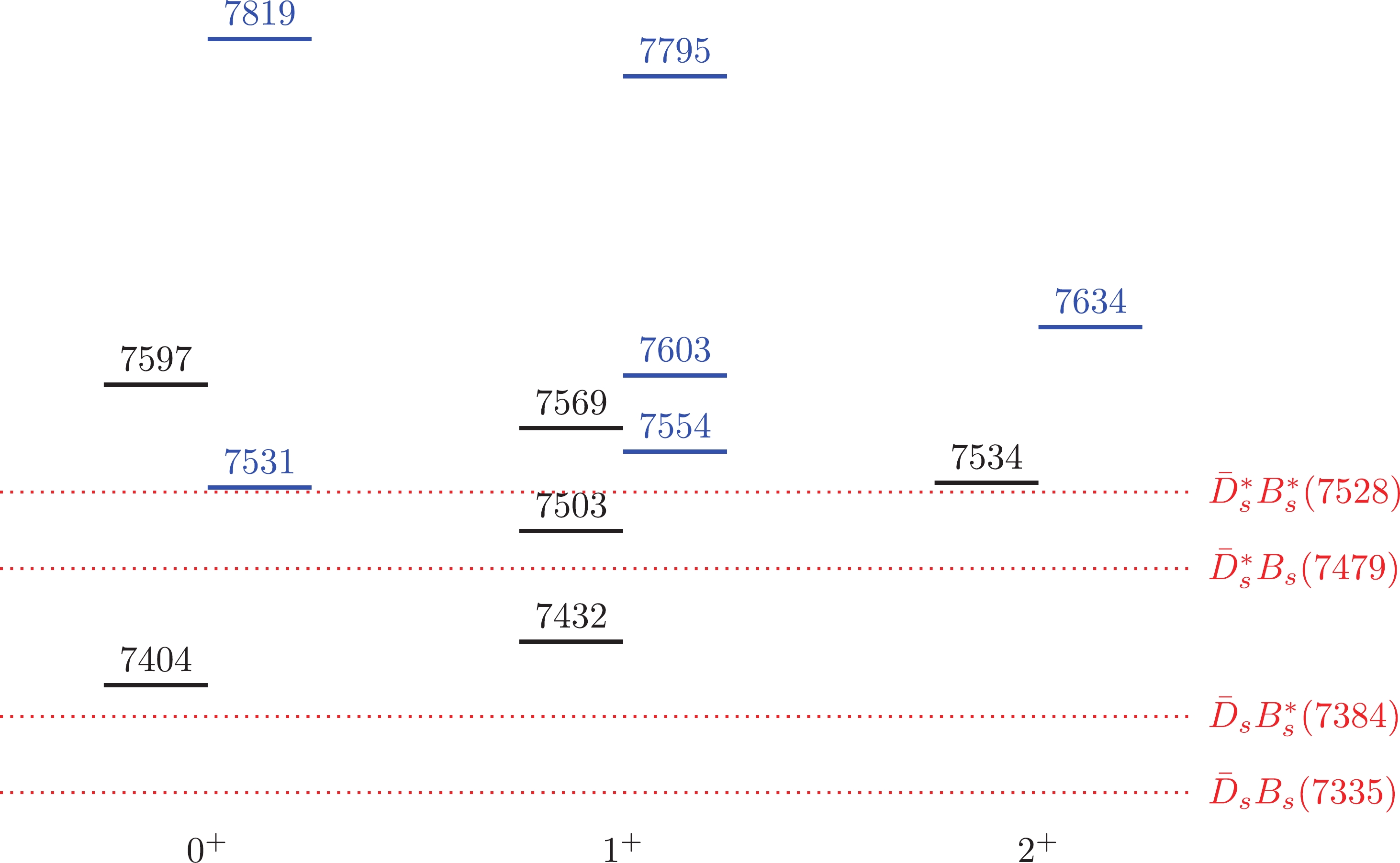
Figure 4. (color online) Mass spectra of the
$ss\bar{c}\bar{b}$ tetraquark states in scheme I (black) and scheme II (blue). The dotted lines indicate various meson-meson thresholds. All masses are in units of MeV.First, we focus on the
$ ss\bar{c}\bar{c} $ tetraquarks. Its ground state is$ T_{I}(ss\bar{c}\bar{c},4043.7,0^{+}) $ . It can decay into the$ \bar{D}_{s}\bar{D}_{s} $ mode in an S-wave, and thus, it might be a wide state. The most heavy state,$ T_{I}(ss\bar{c}\bar{c},4311.1,0^{+}) $ lies above the$ \bar{D}_{s}^{*}\bar{D}_{s}^{*} $ threshold. It decays into the$ \bar{D}_{s}\bar{D}_{s} $ and$ \bar{D}_{s}^{*}\bar{D}_{s}^{*} $ modes with the ratios$ \frac{\Gamma[T_{I}(ss\bar{c}\bar{c},4311.1,0^+){\rightarrow}\bar{D}_{s}\bar{D}_{s}]}{\Gamma[T_{I}(ss\bar{c}\bar{c},4311.1,0^+){\rightarrow}\bar{D}_{s}^{*}\bar{D}_{s}^{*}]} \sim0.0008\,. $

(56) Thus, the
$ \bar{D}_{s}^{*}\bar{D}_{s}^{*} $ mode is dominant. The other two states,$ T_{I}(ss\bar{c}\bar{c},4192.6,1^{+}) $ and$ T_{I}(ss\bar{c}\bar{c},4264.5,2^{+}) $ , can decay into the$ \bar{D}_{s}\bar{D}_{s}^{*} $ and$ \bar{D}_{s}^{*}\bar{D}_{s}^{*} $ modes, respectively.Next, we turn to the
$ ss\bar{b}\bar{b} $ tetraquarks. In scheme I, the$ T_{I}(ss\bar{b}\bar{b},10697.1,0^{+}) $ and$ T_{I}(ss\bar{b}\bar{b},10718.2,1^{+}) $ lie below the$ B_{s}B_{s} $ threshold, and the$ T_{I}(ss\bar{b}\bar{b},10742.5,2^{+}) $ lies just above the$ B_{s}B_{s} $ threshold, which suggests that they are stable states. However, they become heavier than their S-wave decay channels in scheme II. A detailed study with a dynamical model or an experimental study is required to distinguish which of the two schemes provides a better description of the$ ss\bar{b}\bar{b} $ tetraquarks. In both schemes, the three states are dominated by the$ \bar{3}_{c}\otimes3_{c} $ configuration. Actually, their wave functions are nearly the same, except that they have different total spins, which is the reason for their different masses. The highest state can decay into the$ B_{s}B_{s} $ and$ B_{s}^{*}B_{s}^{*} $ modes, with nearly identical partial width ratios$ \frac{\Gamma[T_{I}(ss\bar{b}\bar{b},10928.8,0^+){\rightarrow}B_{s}^{*}B_{s}^{*}]}{\Gamma[T_{I}(ss\bar{b}\bar{b},10928.8,0^+){\rightarrow}B_{s}B_{s}]} \sim4.4 $

(57) and
$ \frac{\Gamma[T_{II}(ss\bar{b}\bar{b},11154.3,0^+){\rightarrow}B_{s}^{*}B_{s}^{*}]}{\Gamma[T_{II}(ss\bar{b}\bar{b},11154.3,0^+){\rightarrow}B_{s}B_{s}]} \sim4.1\,. $

(58) From Fig. 4, we see that all
$ ss\bar{c}\bar{b} $ tetraquarks are above the S-wave decay channels and are probably broad states. Among them, the$ T_{I}(ss\bar{c}\bar{b},7534.3,2^{+}) $ state is slightly above the$ \bar{D}_{s}^{*}B_{s}^{*} $ . Its decay width may be relatively narrow. We also calculate the partial decay width ratios of the$ ss\bar{c}\bar{b} $ tetraquarks. It is interesting that some of the ratios are different in the two schemes. For example, in scheme I$ \frac{\Gamma[T_{I}(ss\bar{c}\bar{b},7597.3,0^+){\rightarrow}\bar{D}_{s}^{*}B_{s}^{*}]}{\Gamma[T_{I}(ss\bar{c}\bar{b},7597.3,0^+){\rightarrow}\bar{D}_{s}B_{s}]} \sim63.2 $

(59) and in scheme II
$ \frac{\Gamma[T_{I}(ss\bar{c}\bar{b},7818.8,0^+){\rightarrow}\bar{D}_{s}^{*}B_{s}^{*}]}{\Gamma[T_{I}(ss\bar{c}\bar{b},7818.8,0^+){\rightarrow}\bar{D}_{s}B_{s}]} \sim9.1\,, $

(60) which can be used to distinguish the two schemes.
-
We list the masses and wave functions of the
$ ns\bar{Q}\bar{Q} $ tetraquarks in Table 24. The ground states of the$ ns\bar{c}\bar{c} $ and$ ns\bar{b}\bar{b} $ tetraquarks are both of$ 1^{+} $ . They are strange counterparts of the$ IJ^{P} = 01^{+} $ $ nn\bar{Q}\bar{Q} $ tetraquarks. Among them, the$ T_{I}(ns\bar{c}\bar{c},3919.0,1^{+}) $ state lies above the$ \bar{D}\bar{D}_{s} $ threshold, whereas the$ T_{I}(ns\bar{b}\bar{b},10473.1,1^{+}) $ state lies deeply below the$ BB_{s} $ threshold. In scheme II, the former one lies above its S-wave decay channels$ \bar{D}^{*}\bar{D}_{s} $ and$ \bar{D}\bar{D}_{s}^{*} $ , whereas the latter one is still stable. We hope that future experiments can aim for this state.System $J^{P}$ 

Scheme I Scheme II Mass Eigenvector Mass Eigenvector $ns\bar{c}\bar{c}$ 

$0^{+}$ 

$3937.6$ 

$\{0.606,0.795\}$ 

$4085.7$ 

$\{0.410,0.912\}$ 

$4209.3$ 

$\{0.795,-0.606\}$ 

$4436.2$ 

$\{0.912,-0.410\}$ 

$1^{+}$ 

$3919.0$ 

$\{-0.534,-0.006,0.845\}$ 

$4051.5$ 

$\{0.284,0.005,-0.959\}$ 

$4073.0$ 

$\{-0.032,-0.999,-0.027\}$ 

$4180.2$ 

$\{0.003,0.99997,0.007\}$ 

$4086.5$ 

$\{0.845,-0.041,0.534\}$ 

$4328.9$ 

$\{0.959,-0.005,0.284\}$ 

$2^{+}$ 

$4144.3$ 

$\{1\}$ 

$4251.5$ 

$\{1\}$ 

$ns\bar{b}\bar{b}$ 

$0^{+}$ 

$10586.4$ 

$\{0.163,0.987\}$ 

$10684.1$ 

$\{0.107,0.994\}$ 

$10854.6$ 

$\{0.987,-0.163\}$ 

$11090.2$ 

$\{0.994,-0.107\}$ 

$1^{+}$ 

$10473.1$ 

$\{0.082,0.005,-0.997\}$ 

$10569.0$ 

$\{0.056,0.005,-0.998\}$ 

$10605.3$ 

$\{0.007,0.99996,0.006\}$ 

$10700.5$ 

$\{0.004,0.99998,0.005\}$ 

$10778.7$ 

$\{0.997,-0.007,0.082\}$ 

$11016.1$ 

$\{0.998,-0.004,0.056\}$ 

$2^{+}$ 

$10628.7$ 

$\{1\}$ 

$10723.9$ 

$\{1\}$ 

$ns\bar{c}\bar{b}$ 

$0^{+}$ 

$7156.5$ 

$\{0.647,0.029,0.038,0.761\}$ 

$7296.2$ 

$\{0.375,0.036,0.050,0.925\}$ 

$7299.0$ 

$\{0.030,0.473,0.876,-0.087\}$ 

$7421.1$ 

$\{0.044,0.283,0.955,-0.080\}$ 

$7333.2$ 

$\{-0.762,0.070,0.052,0.642\}$ 

$7547.8$ 

$\{-0.926,0.055,0.058,0.370\}$ 

$7506.6$ 

$\{-0.023,-0.878,0.477,0.029\}$ 

$7738.5$ 

$\{-0.026,-0.957,0.287,0.032\}$ 

$1^{+}$ 

$7212.8$ 

$\{0.423,-0.343,0.031,0.024,-0.025,0.838\}$ 

$7336.1$ 

$\{0.181,-0.185,0.035,0.023,-0.030,0.965\}$ 

$7323.9$ 

$\{-0.210,0.057,-0.413,-0.589,0.635,0.180\}$ 

$7440.9$ 

$\{-0.044,0.030,-0.225,-0.675,0.698,0.060\}$ 

$7330.5$ 

$\{-0.818,0.168,0.161,0.095,-0.225,0.466\}$ 

$7487.8$ 

$\{-0.089,-0.033,0.041,-0.720,-0.687,0.005\}$ 

$7386.1$ 

$\{0.004,0.224,-0.056,0.749,0.615,0.089\}$ 

$7565.3$ 

$\{0.901,-0.351,-0.047,-0.090,-0.010,-0.233\}$ 

$7416.2$ 

$\{0.329,0.894,0.062,-0.169,-0.144,0.198\}$ 

$7665.0$ 

$\{-0.381,-0.916,-0.042,0.039,0.048,-0.102\}$ 

$7479.9$ 

$\{0.013,-0.040,0.892,-0.233,0.383,-0.038\}$ 

$7716.8$ 

$\{-0.014,0.042,-0.971,0.129,-0.194,0.037\}$ 

$2^{+}$ 

$7415.1$ 

$\{0.297,0.955\}$ 

$7517.7$ 

$\{0.064,0.998\}$ 

$7439.0$ 

$\{0.955,-0.297\}$ 

$7690.6$ 

$\{0.998,-0.064\}$ 

Table 24. Masses and eigenvectors of the
$ns\bar{c}\bar{c}$ ,$ns\bar{b}\bar{b}$ , and$ns\bar{c}\bar{b}$ tetraquarks. All masses are in units of MeV.The last class of the doubly heavy tetraquarks is the
$ ns\bar{c}\bar{b} $ system. It is composed of four different quarks. Similar to the$ nn\bar{c}\bar{b} $ tetraquarks, the ground state of the$ ns\bar{c}\bar{b} $ tetraquarks has quantum number$ 0^{+} $ . Depending on the scheme used, it may be a stable state. A full dynamical quark model study is needed to have a better understanding of these states.We also study the decay properties of the
$ ns\bar{Q}\bar{Q} $ tetraquarks, which can be found in Tables 25-34.System $J^{P}$ 

Scheme I Scheme II Mass $\bar{D}^{*}\bar{D}_{s}^{*}$ 

$\bar{D}^{*}\bar{D}_{s}$ 

$\bar{D}\bar{D}_{s}^{*}$ 

$\bar{D}\bar{D}_{s}$ 

Mass $\bar{D}^{*}\bar{D}_{s}^{*}$ 

$\bar{D}^{*}\bar{D}_{s}$ 

$\bar{D}\bar{D}_{s}^{*}$ 

$\bar{D}\bar{D}_{s}$ 

$ns\bar{c}\bar{c}$ 

$0^{+}$ 

$3937.6$ 

$0.199$ 

$0.645$ 

$4085.7$ 

$0.026$ 

$0.623$ 

$4209.3$ 

$0.737$ 

$0.022$ 

$4436.2$ 

$0.763$ 

$0.168$ 

$1^{+}$ 

$3919.0$ 

$0.036$ 

$-0.464$ 

$0.460$ 

$4051.5$ 

$-0.227$ 

$0.395$ 

$-0.391$ 

$4073.0$ 

$-0.029$ 

$-0.413$ 

$-0.403$ 

$4180.2$ 

$-0.005$ 

$-0.408$ 

$-0.409$ 

$4086.5$ 

$0.706$ 

$0.174$ 

$-0.207$ 

$4328.9$ 

$0.670$ 

$0.307$ 

$-0.311$ 

$2^{+}$ 

$4144.3$ 

$0.577$ 

$4251.5$ 

$0.577$ 

Table 25. Eigenvectors of the
$ns\bar{c}\bar{c}$ tetraquark states in the$n\bar{c}{\otimes}s\bar{c}$ configuration. All masses are in units of MeV.System $J^{P}$ 

Scheme I Scheme II Mass $\bar{D}^{*}\bar{D}_{s}^{*}$ 

$\bar{D}^{*}\bar{D}_{s}$ 

$\bar{D}\bar{D}_{s}^{*}$ 

$\bar{D}\bar{D}_{s}$ 

Mass $\bar{D}^{*}\bar{D}_{s}^{*}$ 

$\bar{D}^{*}\bar{D}_{s}$ 

$\bar{D}\bar{D}_{s}^{*}$ 

$\bar{D}\bar{D}_{s}$ 

$ns\bar{c}\bar{c}$ 

$0^{+}$ 

$3937.6$ 

× $185.3$ 

$4085.7$ 

× $273.5$ 

$4209.3$ 

$233.6$ 

$0.4$ 

$4436.2$ 

$478.6$ 

$31.3$ 

$1^{+}$ 

$3919.0$ 

× × × $4051.5$ 

× $60.4$ 

$58.0$ 

$4073.0$ 

× $75.1$ 

$70.3$ 

$4180.2$ 

$0.008$ 

$107.1$ 

$106.8$ 

$4086.5$ 

× $14.2$ 

$20.0$ 

$4328.9$ 

$297.3$ 

$80.7$ 

$82.5$ 

$2^{+}$ 

$4144.3$ 

$73.7$ 

$4251.5$ 

$174.4$ 

Table 26. Values of
$k\cdot|c_{i}|^2$ for the$ns\bar{c}\bar{c}$ tetraquarks (in units of MeV).System $J^{P}$ 

Scheme I Scheme II Mass $\bar{D}^{*}\bar{D}_{s}^{*}$ 

$\bar{D}^{*}\bar{D}_{s}$ 

$\bar{D}\bar{D}_{s}^{*}$ 

$\bar{D}\bar{D}_{s}$ 

Mass $\bar{D}^{*}\bar{D}_{s}^{*}$ 

$\bar{D}^{*}\bar{D}_{s}$ 

$\bar{D}\bar{D}_{s}^{*}$ 

$\bar{D}\bar{D}_{s}$ 

$ns\bar{c}\bar{c}$ 

$0^{+}$ 

$3937.6$ 

× 1 $4085.7$ 

× 1 $4209.3$ 

$569.1$ 

1 $4436.2$ 

$15.3$ 

1 $1^{+}$ 

$3919.0$ 

× × × $4051.5$ 

× $1.04$ 

1 $4073.0$ 

× $1.1$ 

1 $4180.2$ 

$0.00007$ 

$1.003$ 

1 $4086.5$ 

× $0.7$ 

1 $4328.9$ 

$3.6$ 

$0.98$ 

1 $2^{+}$ 

$4144.3$ 

1 $4251.5$ 

1 Table 27. Partial width ratios for the
$ns\bar{c}\bar{c}$ tetraquarks. For each state, we choose one mode as the reference channel, and the partial width ratios of the other channels are calculated relative to this channel. All masses are in units of MeV.System $J^{P}$ 

Scheme I Scheme II Mass $B^{*}B_{s}^{*}$ 

$B^{*}B_{s}$ 

$BB_{s}^{*}$ 

$BB_{s}$ 

Mass $B^{*}B_{s}^{*}$ 

$B^{*}B_{s}$ 

$BB_{s}^{*}$ 

$BB_{s}$ 

$ns\bar{b}\bar{b}$ 

$0^{+}$ 

$10586.4$ 

$-0.170$ 

$0.560$ 

$10684.1$ 

$-0.212$ 

$0.541$ 

$10854.6$ 

$0.745$ 

$0.321$ 

$11090.2$ 

$0.734$ 

$0.353$ 

$1^{+}$ 

$10473.1$ 

$-0.360$ 

$0.323$ 

$-0.319$ 

$10569.0$ 

$-0.375$ 

$0.313$ 

$-0.309$ 

$10605.3$ 

$-0.006$ 

$-0.409$ 

$-0.407$ 

$10700.5$ 

$-0.004$ 

$-0.408$ 

$-0.408$ 

$10778.7$ 

$0.609$ 

$0.380$ 

$-0.386$ 

$11016.1$ 

$0.599$ 

$0.390$ 

$-0.393$ 

$2^{+}$ 

$10628.7$ 

$0.577$ 

$10723.9$ 

$0.577$ 

Table 28. Eigenvectors of the
$ns\bar{b}\bar{b}$ tetraquark states in the$n\bar{b}{\otimes}s\bar{b}$ configuration. All masses are in units of MeV.System $J^{P}$ 

Scheme I Scheme II Mass $B^{*}B_{s}^{*}$ 

$B^{*}B_{s}$ 

$BB_{s}^{*}$ 

$BB_{s}$ 

Mass $B^{*}B_{s}^{*}$ 

$B^{*}B_{s}$ 

$BB_{s}^{*}$ 

$BB_{s}$ 

$ns\bar{b}\bar{b}$ 

$0^{+}$ 

$10586.4$ 

× × $10684.1$ 

× $131.4$ 

$10854.6$ 

$436.2$ 

$109.4$ 

$11090.2$ 

$744.5$ 

$193.1$ 

$1^{+}$ 

$10473.1$ 

× × × $10569.0$ 

× × × $10605.3$ 

× × × $10700.5$ 

× $36.6$ 

$28.9$ 

$10778.7$ 

$168.9$ 

$99.0$ 

$100.0$ 

$11016.1$ 

$439.9$ 

$201.8$ 

$204.1$ 

$2^{+}$ 

$10628.7$ 

× $10723.9$ 

× Table 29. Values of
$k\cdot|c_{i}|^2$ for the$ns\bar{b}\bar{b}$ tetraquarks (in units of MeV).System $J^{P}$ 

Scheme I Scheme II Mass $B^{*}B_{s}^{*}$ 

$B^{*}B_{s}$ 

$BB_{s}^{*}$ 

$BB_{s}$ 

Mass $B^{*}B_{s}^{*}$ 

$B^{*}B_{s}$ 

$BB_{s}^{*}$ 

$BB_{s}$ 

$ns\bar{b}\bar{b}$ 

$0^{+}$ 

$10586.4$ 

× × $10684.1$ 

× 1 $10854.6$ 

$4.0$ 

1 $11090.2$ 

$3.9$ 

1 $1^{+}$ 

$10473.1$ 

× × × $10569.0$ 

× × × $10605.3$ 

× × × $10700.5$ 

× $1.3$ 

1 $10778.7$ 

$1.7$ 

$1.0$ 

1 $11016.1$ 

$2.2$ 

$1.0$ 

1 $2^{+}$ 

$10628.7$ 

× $10723.9$ 

× Table 30. Partial width ratios for the
$ns\bar{b}\bar{b}$ tetraquarks. For each state, we choose one mode as the reference channel, and the partial width ratios of the other channels are calculated relative to this channel. All masses are in units of MeV.System $J^{P}$ 

Scheme I Scheme II Mass $\bar{D}^{*}B_{s}^{*}$ 

$\bar{D}^{*}B_{s}$ 

$\bar{D}B_{s}^{*}$ 

$\bar{D}B_{s}$ 

Mass $\bar{D}^{*}B_{s}^{*}$ 

$\bar{D}^{*}B_{s}$ 

$\bar{D}B_{s}^{*}$ 

$\bar{D}B_{s}$ 

$ns\bar{c}\bar{b}$ 

$0^{+}$ 

$7156.5$ 

$0.126$ 

$0.708$ 

$7296.2$ 

$-0.320$ 

$-0.572$ 

$7299.0$ 

$-0.026$ 

$-0.627$ 

$7421.1$ 

$0.134$ 

$-0.601$ 

$7333.2$ 

$-0.666$ 

$0.299$ 

$7547.8$ 

$-0.585$ 

$0.496$ 

$7506.6$ 

$-0.735$ 

$-0.128$ 

$7738.5$ 

$-0.733$ 

$-0.256$ 

$1^{+}$ 

$7212.8$ 

$0.152$ 

$-0.148$ 

$0.655$ 

$7336.1$ 

$0.295$ 

$-0.263$ 

$0.491$ 

$7323.9$ 

$0.127$ 

$-0.039$ 

$-0.685$ 

$7440.9$ 

$0.197$ 

$-0.012$ 

$-0.589$ 

$7330.5$ 

$0.289$ 

$-0.630$ 

$-0.237$ 

$7487.8$ 

$-0.273$ 

$-0.575$ 

$-0.115$ 

$7386.1$ 

$0.384$ 

$0.574$ 

$0.042$ 

$7565.3$ 

$-0.329$ 

$0.424$ 

$0.544$ 

$7416.2$ 

$0.574$ 

$0.362$ 

$-0.120$ 

$7665.0$ 

$-0.575$ 

$-0.517$ 

$0.109$ 

$7479.9$ 

$0.633$ 

$-0.346$ 

$0.171$ 

$7716.8$ 

$-0.600$ 

$0.391$ 

$-0.302$ 

$2^{+}$ 

$7415.1$ 

$0.794$ 

$7517.7$ 

$0.629$ 

$7439.0$ 

$0.608$ 

$7690.6$ 

$0.778$ 

Table 31. Eigenvectors of the
$ns\bar{c}\bar{b}$ tetraquark states in the$n\bar{c}{\otimes}s\bar{b}$ configuration. All masses are in units of MeV.System $J^{P}$ 

Scheme I Scheme II Mass $B^{*}\bar{D}_{s}^{*}$ 

$B^{*}\bar{D}_{s}$ 

$B\bar{D}_{s}^{*}$ 

$B\bar{D}_{s}$ 

Mass $B^{*}\bar{D}_{s}^{*}$ 

$B^{*}\bar{D}_{s}$ 

$B\bar{D}_{s}^{*}$ 

$B\bar{D}_{s}$ 

$ns\bar{c}\bar{b}$ 

$0^{+}$ 

$7156.5$ 

$0.107$ 

$0.646$ 

$7296.2$ 

$-0.298$ 

$-0.493$ 

$7299.0$ 

$0.137$ 

$0.635$ 

$7421.1$ 

$-0.018$ 

$0.584$ 

$7333.2$ 

$-0.598$ 

$0.407$ 

$7547.8$ 

$-0.541$ 

$0.599$ 

$7506.6$ 

$0.783$ 

$0.112$ 

$7738.5$ 

$0.786$ 

$0.238$ 

$1^{+}$ 

$7212.8$ 

$-0.136$ 

$0.596$ 

$-0.128$ 

$7336.1$ 

$-0.279$ 

$0.426$ 

$-0.236$ 

$7323.9$ 

$-0.086$ 

$0.500$ 

$-0.261$ 

$7440.9$ 

$0.114$ 

$0.549$ 

$-0.048$ 

$7330.5$ 

$-0.286$ 

$-0.576$ 

$-0.447$ 

$7487.8$ 

$-0.240$ 

$0.042$ 

$0.443$ 

$7386.1$ 

$0.054$ 

$-0.169$ 

$-0.438$ 

$7565.3$ 

$0.266$ 

$0.649$ 

$0.465$ 

$7416.2$ 

$-0.621$ 

$-0.116$ 

$0.634$ 

$7665.0$ 

$0.566$ 

$0.140$ 

$-0.612$ 

$7479.9$ 

$0.710$ 

$-0.146$ 

$0.351$ 

$7716.8$ 

$-0.679$ 

$0.273$ 

$-0.395$ 

$2^{+}$ 

$7415.1$ 

$-0.308$ 

$7517.7$ 

$-0.524$ 

$7439.0$ 

$0.951$ 

$7690.6$ 

$0.852$ 

Table 32. Eigenvectors of the
$ns\bar{c}\bar{b}$ tetraquark states in the$n\bar{b}{\otimes}s\bar{c}$ configuration. All masses are in units of MeV.System $J^{P}$ 

Scheme I Scheme II Mass $\bar{D}^{*}B_{s}^{*}$ 

$\bar{D}^{*}B_{s}$ 

$\bar{D}B_{s}^{*}$ 

$\bar{D}B_{s}$ 

Mass $\bar{D}^{*}B_{s}^{*}$ 

$\bar{D}^{*}B_{s}$ 

$\bar{D}B_{s}^{*}$ 

$\bar{D}B_{s}$ 

$ns\bar{c}\bar{b}$ 

$0^{+}$ 

$7156.5$ 

× × $7296.2$ 

× $136.2$ 

$7299.0$ 

× $167.7$ 

$7421.1$ 

× $263.8$ 

$7333.2$ 

× $47.1$ 

$7547.8$ 

$207.8$ 

$234.9$ 

$7506.6$ 

$267.1$ 

$14.5$ 

$7738.5$ 

$527.0$ 

$80.5$ 

$1^{+}$ 

$7212.8$ 

× × × $7336.1$ 

× × $93.3$ 

$7323.9$ 

× × $159.4$ 

$7440.9$ 

$8.7$ 

$0.07$ 

$232.6$ 

$7330.5$ 

× × $20.6$ 

$7487.8$ 

$32.4$ 

$190.9$ 

$10.2$ 

$7386.1$ 

× $58.5$ 

$1.0$ 

$7565.3$ 

$70.5$ 

$135.6$ 

$267.3$ 

$7416.2$ 

× $45.3$ 

$8.9$ 

$7665.0$ 

$282.4$ 

$250.9$ 

$12.7$ 

$7479.9$ 

$162.8$ 

$66.8$ 

$22.0$ 

$7716.8$ 

$340.3$ 

$156.4$ 

$103.6$ 

$2^{+}$ 

$7415.1$ 

× $7517.7$ 

$208.5$ 

$7439.0$ 

$77.7$ 

$7690.6$ 

$544.2$ 

System $J^{P}$ 

Scheme I Scheme II Mass $B^{*}\bar{D}_{s}^{*}$ 

$B^{*}\bar{D}_{s}$ 

$B\bar{D}_{s}^{*}$ 

$B\bar{D}_{s}$ 

Mass $B^{*}\bar{D}_{s}^{*}$ 

$B^{*}\bar{D}_{s}$ 

$B\bar{D}_{s}^{*}$ 

$B\bar{D}_{s}$ 

$ns\bar{c}\bar{b}$ 

$0^{+}$ 

$7156.5$ 

× × $7296.2$ 

× $90.9$ 

$7299.0$ 

× $155.3$ 

$7421.1$ 

× $243.7$ 

$7333.2$ 

× $82.7$ 

$7547.8$ 

$170.9$ 

$339.5$ 

$7506.6$ 

$282.8$ 

$11.0$ 

$7738.5$ 

$601.5$ 

$69.5$ 

$1^{+}$ 

$7212.8$ 

× × × $7336.1$ 

× $64.1$ 

× $7323.9$ 

× $74.7$ 

× $7440.9$ 

$1.4$ 

$198.4$ 

$0.9$ 

$7330.5$ 

× $109.2$ 

× $7487.8$ 

$22.6$ 

$1.4$ 

$106.4$ 

$7386.1$ 

× $14.8$ 

× $7565.3$ 

$44.6$ 

$379.9$ 

$158.0$ 

$7416.2$ 

× $8.0$ 

$109.6$ 

$7665.0$ 

$269.8$ 

$20.7$ 

$345.5$ 

$7479.9$ 

$182.6$ 

$15.8$ 

$63.8$ 

$7716.8$ 

$431.6$ 

$84.8$ 

$157.8$ 

Continued on next page Table 33. Values of
$k\cdot|c_{i}|^2$ for the$ns\bar{c}\bar{b}$ tetraquarks (in units of MeV).System $J^{P}$ 

Scheme I Scheme II Mass $\bar{D}^{*}B_{s}^{*}$ 

$\bar{D}^{*}B_{s}$ 

$\bar{D}B_{s}^{*}$ 

$\bar{D}B_{s}$ 

Mass $\bar{D}^{*}B_{s}^{*}$ 

$\bar{D}^{*}B_{s}$ 

$\bar{D}B_{s}^{*}$ 

$\bar{D}B_{s}$ 

$ns\bar{c}\bar{b}$ 

$0^{+}$ 

$7156.5$ 

× × $7296.2$ 

× 1 $7299.0$ 

× 1 $7421.1$ 

× 1 $7333.2$ 

× 1 $7547.8$ 

$0.9$ 

1 $7506.6$ 

$18.4$ 

1 $7738.5$ 

$6.6$ 

1 $1^{+}$ 

$7212.8$ 

× × × $7336.1$ 

× × 1 $7323.9$ 

× × 1 $7440.9$ 

$0.04$ 

$0.0003$ 

1 $7330.5$ 

× × 1 $7487.8$ 

$3.2$ 

$18.8$ 

1 $7386.1$ 

× $61.5$ 

1 $7565.3$ 

$0.3$ 

$0.5$ 

1 $7416.2$ 

× $5.1$ 

1 $7665.0$ 

$22.3$ 

$19.8$ 

1 $7479.9$ 

$7.4$ 

$3.0$ 

1 $7716.8$ 

$3.3$ 

$1.5$ 

1 $2^{+}$ 

$7415.1$ 

× $7517.7$ 

1 $7439.0$ 

1 $7690.6$ 

1 System $J^{P}$ 

Scheme I Scheme II Mass $B^{*}\bar{D}_{s}^{*}$ 

$B^{*}\bar{D}_{s}$ 

$B\bar{D}_{s}^{*}$ 

$B\bar{D}_{s}$ 

Mass $B^{*}\bar{D}_{s}^{*}$ 

$B^{*}\bar{D}_{s}$ 

$B\bar{D}_{s}^{*}$ 

$B\bar{D}_{s}$ 

$ns\bar{c}\bar{b}$ 

$0^{+}$ 

$7156.5$ 

× × $7296.2$ 

× 1 $7299.0$ 

× 1 $7421.1$ 

× 1 $7333.2$ 

× 1 $7547.8$ 

$0.5$ 

1 $7506.6$ 

$25.8$ 

1 $7738.5$ 

$8.7$ 

1 $1^{+}$ 

$7212.8$ 

× × × $7336.1$ 

× 1 × $7323.9$ 

× 1 × $7440.9$ 

$0.007$ 

1 $0.005$ 

$7330.5$ 

× 1 × $7487.8$ 

$16.7$ 

1 $78.4$ 

$7386.1$ 

× 1 × $7565.3$ 

$0.1$ 

1 $0.4$ 

$7416.2$ 

× 1 $13.6$ 

$7665.0$ 

$13.0$ 

1 $16.7$ 

$7479.9$ 

$11.5$ 

1 $4.0$ 

$7716.8$ 

$5.1$ 

1 $1.9$ 

$2^{+}$ 

$7415.1$ 

× $7517.7$ 

1 $7439.0$ 

1 $7690.6$ 

1 Table 34. Partial width ratios for the
$ns\bar{c}\bar{b}$ tetraquarks. For each state, we choose one mode as the reference channel, and the partial width ratios of the other channels are calculated relative to this channel. All masses are in units of MeV.Table 33-continued from previous page System $J^{P}$ 

Scheme I Scheme II Mass $B^{*}\bar{D}_{s}^{*}$ 

$B^{*}\bar{D}_{s}$ 

$B\bar{D}_{s}^{*}$ 

$B\bar{D}_{s}$ 

Mass $B^{*}\bar{D}_{s}^{*}$ 

$B^{*}\bar{D}_{s}$ 

$B\bar{D}_{s}^{*}$ 

$B\bar{D}_{s}$ 

$2^{+}$ 

$7415.1$ 

× $7517.7$ 

$136.4$ 

$7439.0$ 

$75.0$ 

$7690.6$ 

$646.2$ 

-
In this work, we systematically study the mass spectra of the doubly heavy
$ qq\bar{Q}\bar{Q} $ tetraquarks in the framework of an extended CM model. In addition to the CM interaction, the effect of the color interaction is considered in this model. The model parameters are fitted from the mesons and baryons. Because the spatial configurations of the$ qq $ ($ \bar{q}\bar{q} $ ) and$ q\bar{q} $ pairs are different in the conventional hadrons and tetraquarks, applying these parameters to tetraquarks may cause errors. To appreciate this uncertainty, we adopt two schemes of parameters to study the$ qq\bar{Q}\bar{Q} $ tetraquarks. As indicated in Eq. (41), scheme II obtains larger masses than scheme I. However, the wave functions and decay properties of the two schemes are very similar for the$ qq\bar{Q}\bar{Q} $ tetraquarks. We find three states that are stable in both schemes. They are the$ nn\bar{b}\bar{b} $ tetraquark with quantum number$ IJ^{P} = 01^{+} $ ,$ nn\bar{c}\bar{b} $ tetraquark with quantum number$ IJ^{P} = 00^{+} $ , and$ ns\bar{b}\bar{b} $ tetraquark with quantum number$ J^{P} = 1^{+} $ . They all lie below the thresholds of two pseudoscalar mesons, which can only decay through weak processes. Meanwhile, many narrow states that lie below the S-wave decay channels are also found. It shall be interesting to search for these states.Tetraquarks have two possible color configurations, namely the color-sextet configuration,
$ \left| {(qq)^{6_{c}}(\bar{Q}\bar{Q})^{\bar{6}_{c}}} \right\rangle $ , and the color-triplet one,$ \left| {(qq)^{\bar{3}_{c}}(\bar{Q}\bar{Q})^{3_{c}}} \right\rangle $ . Unlike the fully heavy tetraquarks, the ground states of the doubly heavy tetraquarks favor the color-triplet configurations. Combining the results of the fully and doubly heavy tetraquarks, we can clearly see the trend that the color-triplet configuration becomes more and more important when the mass ratio between the quarks and antiquarks increases.Besides the mass spectra, we estimate the decay properties of the tetraquarks. We hope these states can be searched for in future experiments.
-
X. Z. W. is grateful to Marek Karliner and Guang-Juan Wang for helpful comments and discussions.
-
To calculate the partial decay rates, we need to construct the tetraquark wave functions in the
$ q\bar{q}{\otimes}q\bar{q} $ configuration. The possible color-spin wave functions,$ \{\beta_{i}^{J}\} $ , are listed as follows:1.
$ J^{P} = 0^{+} $ $\tag{A1} \begin{aligned}[b] \beta_{1}^{0} =& \left| {\left(q_{1}\bar{q}_{3}\right)^{8}_{1}\left(q_{2}\bar{q}_{4}\right)^{8}_{1}} \right\rangle _{0} \quad \beta_{2}^{0} = \left| {\left(q_{1}\bar{q}_{3}\right)^{8}_{0}\left(q_{2}\bar{q}_{4}\right)^{8}_{0}} \right\rangle _{0} \\ \beta_{3}^{0} =& \left| {\left(q_{1}\bar{q}_{3}\right)^{1}_{1}\left(q_{2}\bar{q}_{4}\right)^{1}_{1}} \right\rangle _{0} \quad \beta_{3}^{0} = \left| {\left(q_{1}\bar{q}_{3}\right)^{1}_{0}\left(q_{2}\bar{q}_{4}\right)^{1}_{0}} \right\rangle _{0} \end{aligned}$

2.
$ J^{P} = 1^{+} $ $ \begin{aligned}[b] \beta_{1}^{1} =& \left| {\left(q_{1}\bar{q}_{3}\right)^{8}_{1}\left(q_{2}\bar{q}_{4}\right)^{8}_{1}} \right\rangle _{1} \quad \beta_{2}^{1} = \left| {\left(q_{1}\bar{q}_{3}\right)^{8}_{1}\left(q_{2}\bar{q}_{4}\right)^{8}_{0}} \right\rangle _{1} \end{aligned}$

$\tag{A2} \begin{aligned}[b] \beta_{3}^{1} =& \left| {\left(q_{1}\bar{q}_{3}\right)^{8}_{0}\left(q_{2}\bar{q}_{4}\right)^{8}_{1}} \right\rangle _{1} \quad \beta_{4}^{1} = \left| {\left(q_{1}\bar{q}_{3}\right)^{1}_{1}\left(q_{2}\bar{q}_{4}\right)^{1}_{1}} \right\rangle _{1} \\ \beta_{5}^{1} =& \left| {\left(q_{1}\bar{q}_{3}\right)^{1}_{1}\left(q_{2}\bar{q}_{4}\right)^{1}_{0}} \right\rangle _{1} \quad \beta_{6}^{1} = \left| {\left(q_{1}\bar{q}_{3}\right)^{1}_{0}\left(q_{2}\bar{q}_{4}\right)^{1}_{1}} \right\rangle _{1} \end{aligned}$

3.
$ J^{P} = 2^{+} $ $\tag{A3} \begin{aligned}[b] \beta_{1}^{2} = \left| {\left(q_{1}\bar{q}_{3}\right)^{8}_{1}\left(q_{2}\bar{q}_{4}\right)^{8}_{1}} \right\rangle _{2} \quad \beta_{2}^{2} = \left| {\left(q_{1}\bar{q}_{3}\right)^{1}_{1}\left(q_{2}\bar{q}_{4}\right)^{1}_{1}} \right\rangle _{2} \end{aligned} $

where the superscript 1 or 8 denotes the color, and the subscript 0, 1, or 2 denotes the spin. Among them, the
$ 1_{c}{\otimes}1_{c} $ bases can also be written as combinations of two mesons. For example,$ \left| {\left(n_{1}\bar{c}_{3}\right)^{1}_{1}\left(n_{2}\bar{c}_{4}\right)^{1}_{1}} \right\rangle _{J} {\equiv}\left| {\bar{D}^{*}\bar{D}^{*}} \right\rangle _{J} $ .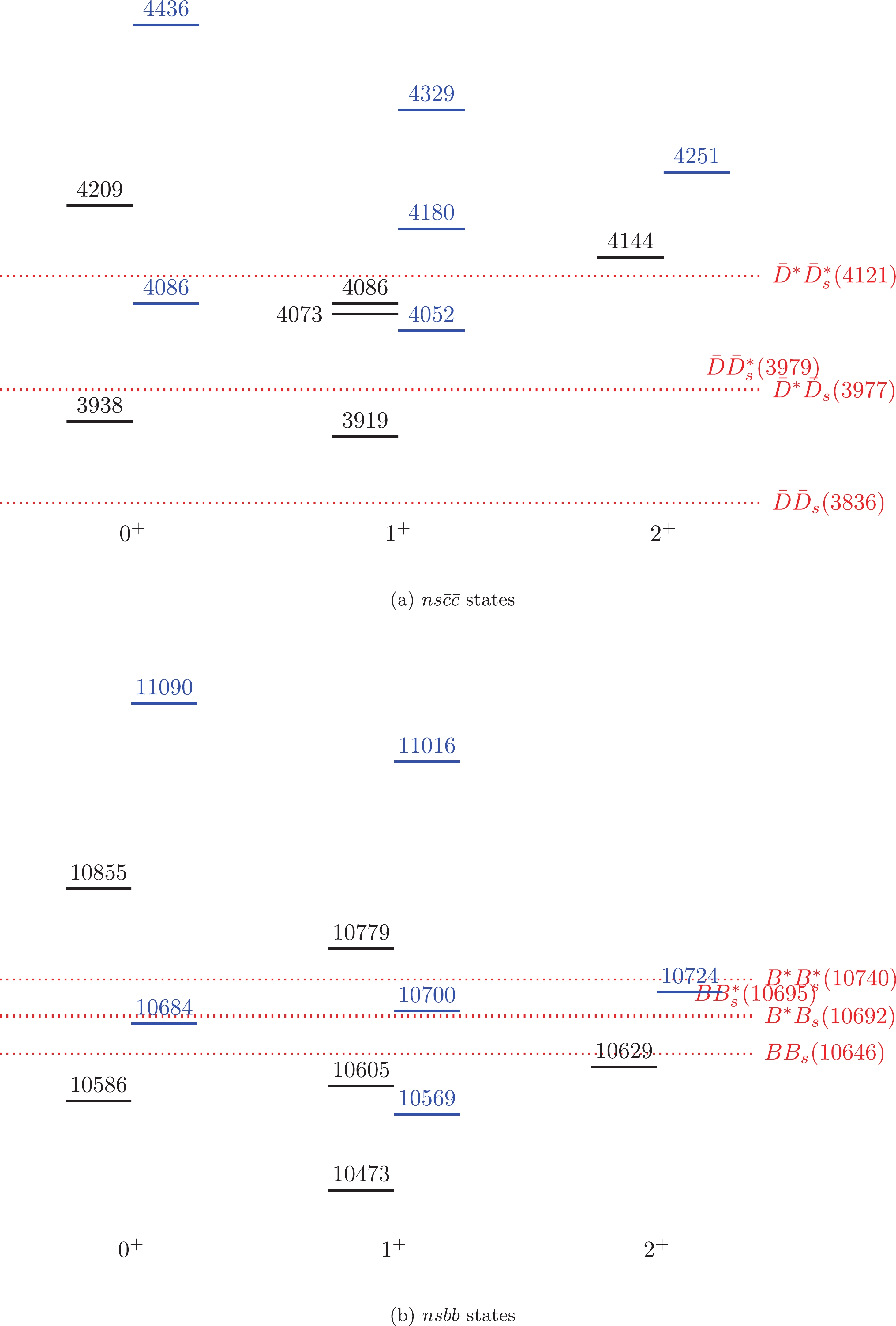
Figure 5. (color online) Mass spectra of the
$ns\bar{c}\bar{c}$ and$ns\bar{b}\bar{b}$ tetraquark states in scheme I (black) and scheme II (blue). The dotted lines indicate various meson-meson thresholds. All masses are in units of MeV.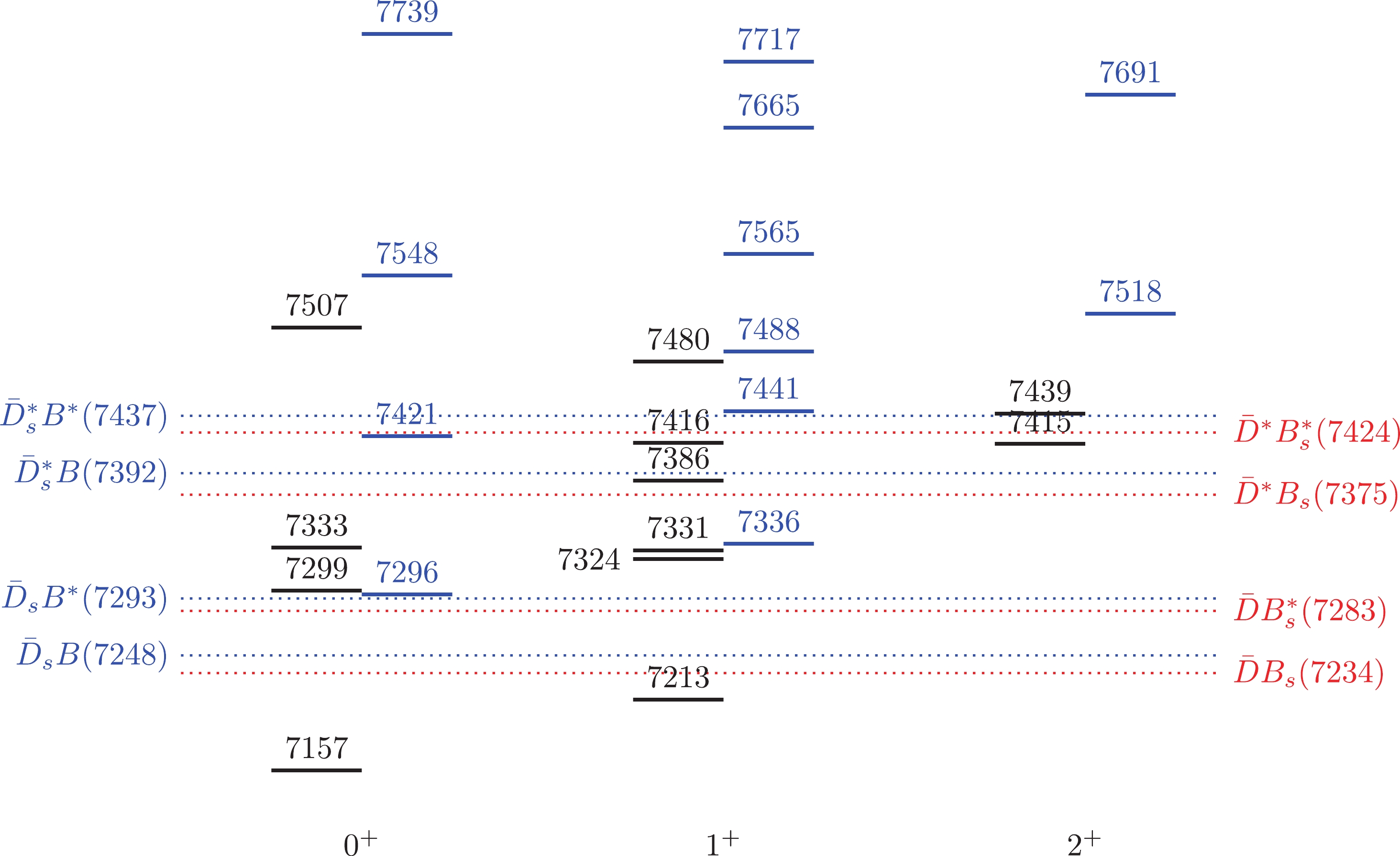
Figure 6. (color online) Mass spectra of the
$ns\bar{c}\bar{b}$ tetraquark states in scheme I (black) and scheme II (blue). The dotted lines indicate various meson-meson thresholds. All masses are in units of MeV.
Doubly heavy tetraquarks in an extended chromomagnetic model
- Received Date: 2021-09-21
- Available Online: 2022-01-15
Abstract: Using an extended chromomagnetic model, we perform a systematic study of the masses of doubly heavy tetraquarks. We find that the ground states of the doubly heavy tetraquarks are dominated by the color-triplet


 DownLoad: