Weak decays of ${\boldsymbol \Xi^{(')}_{\boldsymbol c}\to \boldsymbol\Xi }$ in the light-front quark model

Recently, the Belle Collaboration measured the branching fraction of the semi-leptonic decay of the charmed baryon $ \Xi_c $ as $ {\cal{B}}({\Xi^0}_c\to \Xi^- e^+\nu_e) = (1.72\pm0.10\pm $$ 0.12\pm0.50)% $ [1], where the first and second uncertainties are statistical and systematic whereas the third one arises from the uncertainty of $ {\cal{B}}({\Xi^0}_c\to \Xi^- \pi^+) = (1.80\pm0.52) % $ measured also by the Belle collaboration [2]. In 1993, the ARGUS Collaboration [3] first observed the $ {\Xi^0}_c\to \Xi^- e^+\nu_e $ decay and in 1995 the CLEO Collaboration [4] discovered the $ {\Xi^0}_c\to \Xi^- e^+\nu_e $ events. In addition, the ratio $ {\cal{B}}({\Xi^0}_c\to $$ \Xi^- e^+\nu_e)/{\cal{B}}({\Xi^0}_c\to \Xi^- \pi^+) $ was measured to be $ 0.96\pm0.43\pm0.18 $ by ARGUS and $ 3.1\pm1.0^{+0.3}_{-0.5} $ by CLEO. With the data $ {\cal{B}}({\Xi^0}_c\to \Xi^- \pi^+) = $$ (1.80\pm0.52)% $, the previous average of $ {\cal{B}}({\Xi^0}_c\to \Xi^- e^+\nu_e) $ was calculated as $ (2.34\pm 1.59)% $ [5]. Apparently, the measurement of the Belle Collaboration on $ {\cal{B}}({\Xi^0}_c\to \Xi^- e^+\nu_e) $ is more precise at present. Recently, a lattice calculation was performed on $ {\cal{B}}({\Xi^0}_c\to \Xi^- e^+\nu_e) $ [6], resulting in $ (2.29\pm0.29\pm $$ 0.31)% $. Some theoretical predictions based on different phenomenological models have been given as $ (3.4\pm0.7)% $ [7], $ (3.49\pm0.95)% $ [8], $ (7.26\pm2.54)% $ [9], $ 1.35% $ [10], $ (4.87\pm1.74)% $ [11], $ (2.4\pm0.3)% $ [12], and $ 2.38% $ [13]. Therefore, the precision of theoretical evaluations should be further improved.

In this study, we employed the light-front quark model to analyze the weak decays of $ \Xi^{(')}_{c}\to \Xi $. The light-front quark model (LFQM) is a relativistic quark model that has been applied to study transitions among mesons. Relevant theoretical predictions with this model agree with the experimental data within reasonable error tolerance [14-30]. Later, the model was extended to study the decays of pentaquark within the diquark-diquark-antiquark picture [31, 32] and the weak decay of baryons in the quark-diquark picture [33-39]. With this model, we employed the three-body vertex function to explore the decays of $ \Lambda_b $ and $ \Sigma_b $ [40], where three individual quarks are concerned. The related picture is somewhat different from the structure in which one-diquark and one-quark are basic constituents. Geng et al. [8] also studied the decay of baryons under the three-quark picture in a light front quark model. They followed an approach different from ours to address the flavor-spin wave function of baryons. Note that in the three-body structure, even though two quarks might be loosely bound as a subsystem with definite spin and color, unlike the diquark, which is a relatively stable subject, the subsystem may break and its components would undergo a re-combination with other quarks to constitute different sub-systems, especially after a hadronic transition.

In the three-body vertex function of baryon, two quarks join together into a subsystem that has a definite spin. Then, the subsystem couples with the remaining quark to form a baryon with the defined spin. To evaluate the transition between two baryons, we first need to know the inner spin structures of the concerned baryons. For single charmed-baryons $ \Xi_c $ and $ \Xi'_c $, the two light quarks $ sq $, where $ q $ denotes $ u $ or $ d $ quark, can be regarded as a subsystem with definite spin (similar to a diquark) [41, 42]. By contrast, there are three light quarks in $ \Xi $, where two $ s $ quarks possess definite spin 1 owing to the antisymmetry of the total wave function; thus, they can be regarded as a subsystem. In the transition $ \Xi^{(')}_{c}\to\Xi $, the $ c $ quark in the initial state would transit into an $ s $ quark by emitting a gauge boson, and the original $ sq $ pair can be regarded as a spectator that does not undergo any changes during the hadronic transition. However, in the final state, the newly emerged $ s $ quark is a decay product of the initial $ c $ quark and couples to the original $ s $ quark to form a physical $ ss $ subsystem with definite spin. Thus, the $ sq $ from the initial state is no longer a physical subsystem. In other words, the old subsystem $ sq $ is broken and a new subsystem $ ss $ emerges during the hadronic transition. Definitely, we would account for the changes of constituents in the subsystems as caused by a non-perturbative QCD effect. Nevertheless, the $ ss $ subsystem is not a spectator because one of the $ s $ quarks originates from weak decay of the initial $ c $ quark. Therefore, the simple quark-diquark picture does not apply to these processes. To use the spectator approximation, the ($ ss $)-($ q $) structure must be rearranged into the $ s $-($ sq $) structure through a Racah transformation.

This paper is organized as follows: after the introduction, in Section II we deduce the transition amplitude for $ \Xi^{(')}_{c}\rightarrow \Xi $ in the light-front quark model and provide the expressions of the form factors. Then, we present numerical results for $ \Xi^{(')}_{c}\rightarrow \Xi $ in Section III. Section IV is devoted to the conclusion and discussions.

Enlightened by Ref. [43], in our previous study [40], we constructed the vertex functions of baryons under the three-quark picture, in which two quarks constitute a subsystem with definite spin, and then the subsystem couples with the rest quark to form a baryon. We employed the vertex functions to study the decays of $ \Lambda_b $ and $ \Sigma_b $ [40]. Later, we employed the three-quark vertex functions to study the transition $ \Xi_{cc}\to \Xi_c $ [44]. The success encouraged us to apply this procedure to further study relevant processes.

Similar to Ref. [40], the vertex functions of $ \Xi_{c} $, $ \Xi'_{c} $ and $ \Xi $ with total spin $ S = 1/2 $ and momentum $ P $ are

Let us repeat some details about the three-body function because it plays a key role in our calculations. To obtain the expression of $ \Psi^{SS_z}_{\Xi_{c}^{(')}} $ and $ \Psi^{SS_z}_{\Xi} $, one needs to know their inner spin-flavor structure. In Ref. [42], the $ sq $ in $ \Xi_{c} $ is considered as a scalar subsystem whereas in $ \Xi'_{c} $, it is a vector. In the decay process of $ \Xi^{(')}_{c}\to\Xi $, the $ c $ quark transits into an $ s $ quark via weak interaction and the original $ sq $ subsystem can be approximately regarded as a spectator because it does not undergo any change during the hadronic transition. However, the two strange quarks in $ \Xi $ compose a physical subsystem with a spin of 1. To apply the spectator approximation for the transition, we rearrange the quark structure of $ (ss) $-$ q $ into a sum of $ \sum_i s $-$ (sq)_i $ where $ i $ runs over all possible spin projections by a Racah transformation. With the rearrangement of the quark spin-flavor, the physical structure $ (ss) $-$ q $ in $ \Xi $ is rewritten into a sum over the effective structures of $ s $-$ (sq) $. The detailed transformations are [37]

and then

with [40, 43]

where $ p_1 $ is the the momentum of the newly emerged $ s $ quark in the transition; $ \,p_2\,,p_3 $ are the momenta of the spectator quarks $ s $ and $ q $, respectively; $ U $ and $ V $ are spinors; and $ \lambda_1,\lambda_2, \lambda_3 $ are the helicities of the constituents. Given that the spin of the $ sq $ subsystem is 0 (1), the expressions of $ \Psi^{SS_z}_{\Xi_{c}} $ ($ \Psi^{SS_z}_{\Xi_{c}^{'}} $) are the same as $ \Psi^{SS_z}_0 $ ($ \Psi^{SS_z}_1 $) except for $ p_1 $, which is the momentum of the $ c $ quark.

The spatial wave function is denoted as

with $\varphi(\overrightarrow{k},\beta) = 4\left(\dfrac{\pi}{\beta^2}\right)^{3/4}{\rm exp}\left(\dfrac{-k_z^2-k^2_\perp}{2\beta^2}\right)$.

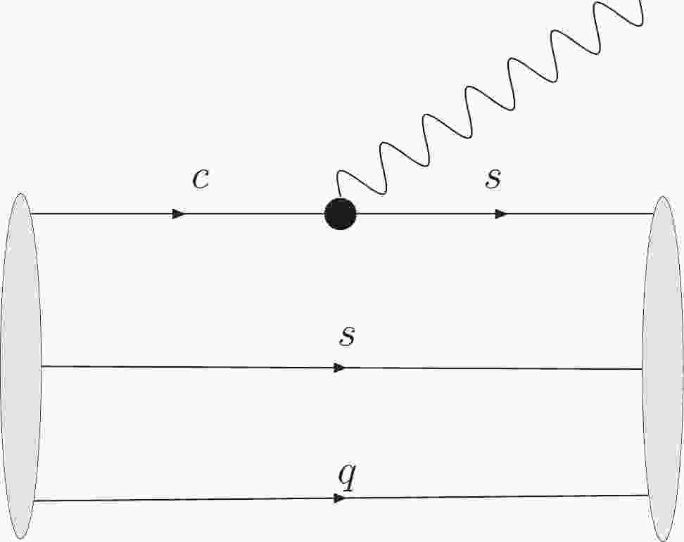
First, we considered the weak decay $ \Xi_{c}\to\Xi $. The leading order Feynman diagram is depicted in Fig. 1. Following the procedures given in Refs. [31-33], the transition matrix element can be evaluated with the vertex functions of $ \mid \Xi_{c}(P,S,S_z) \rangle $ and $ \mid \Xi^(P',S',S'_z) \rangle $. The $ sq $ subsystem behaves as a spectator, i.e., its spin-flavor configuration does not change during the transition; therefore, only the first term in Eq. (4) can contribute to the transition. The hadronic matrix element can be denoted as

Figure 1.  (color online) Feynman diagram for $ \Xi^{(')}_{c}\to\Xi $ transition, where $ \bullet $ and $ q $ denote $ V-A $ current vertex and $ u $ or $ d $ quark respectively.

where

where $ P $($ P' $) is the four-momentum of $ \Xi_{c} $($ \Xi $) and $ M $($ M' $) is the mass of $ \Xi_{c} $ ($ \Xi $). Setting $ \tilde{p}_1 = \tilde{p}'_1+\tilde{Q} $, $ \tilde{p}_2 = \tilde{p}'_2 $, and $ \tilde{p}_3 = \tilde{p}'_3 $, we get

The form factors for the weak transition, $ \Xi_{c}\rightarrow \Xi $, are defined in the standard way as

where $ Q \equiv P-P' $. Similarly, one can express the transition matrix of $ \Xi'_{c}\rightarrow \Xi $ whose form factors are denoted as $ f_i^v $ and $ g_i^v $.

The detailed expressions of the form factors are

These form factors are the same as those reported in our previous paper [40] except for an additional factor $ -\dfrac{\sqrt{3}}{2} $ or $ \dfrac{1}{2} $, which exists in the corresponding equations of the equation group (4).

To study the transitions $ \Xi_{c}\to \Xi $ and $ \Xi'_{c}\to \Xi $, the aforementioned form factors must be calculated numerically; the parameters in the model should be pre-determined. The lifetime of $ \Xi_{c} $ and the masses of $ \Xi_{c} $, $ \Xi'_{c} $, and $ \Xi $ were taken from the data book of particle data group [5]. The masses of quarks given in Ref. [45] are collected in Table 1. We still know little about parameters $ \beta_1 $, $ \beta_{23} $, $ \beta_1' $, and $ \beta_{23}' $ in the wave function for the initial and final baryons. Generally, the reciprocal of $ \beta $ is related to the electrical radius of meson with two constituents. Given that the strong coupling between $ q $ and $ q^{(')} $ is half that between $ q\bar q^{(')} $, for a Coulomb-like interaction, if the two interactions are equal, one can expect the electrical separation of $ q $ and $ q^{(')} $ to be $ 1/\sqrt{2} $ times that of $ q $ and $ \bar q^{(')} $, i.e., $ \beta_{qq^{(')}}\approx\sqrt{2}\beta_{q\bar q^{(')}} $. By considering the binding energy, the authors of Ref. [46] obtained the same results. In our previous paper, for a compact $ q q^{(')} $ system, we found $ \beta_{qq^{(')}} = 2.9\beta_{q\bar q^{(')}} $. Given that the $ sq $ subsystem is easy to break, we assumed it is not a compact system and estimated $ \beta_{c[sq]}\approx \sqrt{2}\beta_{c\bar s} $ and $ \beta_{[sq]}\approx \sqrt{2}\beta_{s\bar q} $, where $ \beta_{c\bar s} $ and $ \beta_{s\bar q} $ were obtained for the meson case [45]. Concerning $ ss $, we do not know whether it is a compact system, and thus we let $ \beta_{s[sq]} $ be a free parameter to fix the data of $ {\Xi^0}_c\to \Xi^- e^+\nu_e $. With these parameters, we calculated the form factors and the transition rates theoretically.

$ m_c $	$ m_s $	$ m_{u} $	$ \beta_{c[sq]} $	$ \beta_{s[sq]} $	$ \beta_{[cu]} $
$ 1.5 $	$ 0.5 $	0.25	0.699	1.07	0.546

Table 1.  Quark mass and parameter $ \beta $ (in units of GeV).

Form factors $ f^{s}_i $, $ g^{s}_i $, $ f^{v}_i $, and $ g^{v}_i\,{(i = 1,2)} $, were evaluated in the space-like region ( $ Q^+ = 0 $ i.e. $ Q^2 = -Q^2_{\perp}\leqslant 0 $), and therefore should be analytically extrapolated to the time-like region. In Ref. [32], the authors employed a three-parameter form

where $ F(Q^2) $ represents $ f^{s}_i $, $ g^{s}_i $, $ f^{v}_i $, and $ g^{v}_i\,{(i = 1,2)} $. Using the numerical form factors evaluated in the space-like region, we may fix the parameters $ a,\; b $ and $ F(0) $ in the un-physical region. When one uses Eq. (13) at the $ Q^2\geqslant 0 $ region, these form factors are extended into the physical region. Letting the model parameters (the quark masses and all $ \beta $s) fluctuate up to $ \pm $10%, we estimated the theoretical uncertainties in our numerical results. The values of $ a,\; b $ and $ F(0) $ for the form factors $ f_{1} $, $ f_{1} $, $ g_{1} $, and $ g_{2} $ are listed in Table 2. The dependence of the form factors (central values) on $ Q^2 $ is depicted in Fig. 2. The values of $ F(0) $ in several previous studies are listed in Table 3. They deviate from each other as shown. The differences in $ f^s_1 $, $ f^s_2 $, and $ g^s_1 $ in Refs. [7, 8, 10, 13] are not very significant but that of $ g^s_2 $ is. The values of $ f^v_1 $, $ f^v_2 $, $ g^v_1 $, and $ g^v_2 $ at $ Q^2 = 0 $ can be found in Ref. [9]; they notably differ from our calculated values.

$ F $	$ F(0) $	$ a $	$ b $
$ f^s_1 $	$ -0.640\pm0.045 $	$ 0.711\pm0.152 $	$ 0.0981\pm0.0386 $
$ f^s_2 $	$ -0.366\pm0.045 $	$ 1.07\pm0.22 $	$ 0.295\pm0.105 $
$ g^s_1 $	$ -0.515\pm0.032 $	$ 0.471\pm0.116 $	$ 0.0839\pm0.0232 $
$ g^s_2 $	$ -0.117\pm0.0349 $	$ 1.31\pm0.260 $	$ 0.381\pm0.127 $
$ f^v_1 $	$ 0.373\pm0.028 $	$ 1.29\pm0.18 $	$ 0.499\pm0.14 $
$ f^v_2 $	$ -0.259\pm0.025 $	$ 1.26\pm0.19 $	$ 0.425\pm0.12 $
$ g^v_1 $	$ -0.0990\pm0.0059 $	$ 0.458\pm0.119 $	$ 0.312\pm0.096 $
$ g^v_2 $	$ 0.0214\pm0.0045 $	$ 0.989\pm0.242 $	$ 0.938\pm0.372 $

Table 2.  Form factors given in the three-parameter forms.

Figure 2.  (color online) Dependence of form factors (central values) $ f^s_1 $, $ f^s_2 $, $ g^s_1 $, and $ g^s_2 $ in a three-parameter form on $ Q^2 $ (a) and dependence of the form factors (central values) $ f^v_1 $, $ f^v_2 $, $ g^v_1 $, and $ g^v_2 $ on $ Q^2 $ (b).

$ F(0) $	this study	Ref. [7]	Ref. [8]	Ref. [9]	Ref. [10]	Ref. [13]
$ f^s_1(0) $	−0.640	−0.71	0.77	0.194	−0.567	0.590
$ f^s_2(0) $	−0.366	−0.46	0.96	0.356	−0.305	0.441
$ g^s_1(0) $	−0.515	−0.71	0.69	0.311	−0.491	0.582
$ g^s_2(0) $	−0.117	−0.14	0.0068	0.151	−0.046	−0.184
$ f^v_1(0) $	0.373	−	−	0.577	−	−
$ f^v_2(0) $	−0.259	−	−	0.501	−	−
$ g^v_1(0) $	−0.0990	−	−	0.451	−	−
$ g^v_2(0) $	0.0214	−	−	0.341	−	−

Table 3.  Form factors (central values) at $ Q^2 = 0 $ reported in different studies.

Using the central value of the data $ \Xi^0_{c} \to \Xi^- e^+\bar{\nu}_e $ from the Belle measurements [5], we fixed the parameter $ \beta_{s[sd]} $. In particular, we first assigned $ \beta_{s[sd]} $ a value and then calculated form factors $ f^s_1 $, $ f^s_2 $, $ g^s_1 $, and $ g^s_2 $ to obtain the theoretical prediction on the rate for $ \Xi^0_{c} \to \Xi^- e^+\bar{\nu}_e $. Then, we compared the theoretical estimates of $ BR(\Xi^0_{c} \to \Xi^- e^+\bar{\nu}_e) $ with the data. A deviation would have required us to modify the parameter, repeating the procedure until they became equal to each other. Thus, we fixed $ \beta_{s[sd]} $ to 1.07 GeV, which is 2.9 times larger than $ \beta_{s\bar s} = 0.366 $ GeV. This value may imply that the $ ss $ pair in $ \Xi $ is a more compact subsystem. With the same parameters, the form factors $ f^v_1 $, $ f^v_2 $, $ g^v_1 $, and $ g^v_2 $ can be obtained. We also evaluated the rate of $ \Xi'_{c} \to \Xi l\bar{\nu}_l $. The differential decay widths of $ {\rm d}\Gamma/{\rm d}\omega $ ($ \omega = \dfrac{P\cdot P'}{MM'} $) are shown in Fig. 3 (corresponding to the central values of the form factors).

Figure 3.  (color online) Differential decay rates $ {\rm d}\Gamma/{\rm d}\omega $ for the decay $ \Xi_{c} \to \Xi l\bar{\nu}_l $(a) and $ \Xi'_{c} \to \Xi l\bar{\nu}_l $ (b).

Our numerical results on the decay widths and the ratio of the longitudinal versus transverse decay rates $ R $ (see its expression in Appendix) of $ \Xi^0_{c} \to \Xi^- e^+\bar{\nu}_e $ and $ \Xi^+_{c} \to \Xi^0 e^+\bar{\nu}_e $ are all presented in Table 4. Some predictions on the same channels are also presented in Table 4. One may notice that the prediction on $ \Gamma(\Xi^0_{c} \to \Xi^- e^+\bar{\nu}_e) $ given by the author of Ref. [10] is close to our results but his prediction on the branching ratio is lower than the central value of data because the measured lifetime of $ \Xi^0_{c} $ [5, 47] significantly varied since the study [10] was reported. The values of $ R $ given in Refs. [7, 10] are lower than ours. Table 5 presents the predictions on $ \Xi'_{c} \to \Xi l\bar{\nu}_l $. Given that form factors $ f^v_1 $, $ f^v_2 $, $ g^v_1 $, and $ g^v_2 $ in Ref. [9] deviate from ours significantly, the width of $ \Xi'_{c} \to \Xi l\bar{\nu}_l $ that they obtained is two orders of magnitude larger than ours. This should also be tested through more precise measurements in the future.

	$ \Gamma $/($ 10^{-12}{\rm GeV} $)	$ {\cal{B}} $	R	$ \Gamma $/($ 10^{-12}{\rm GeV} $)	$ {\cal{B}} $	$ R $
this work	0.0740$ \pm $0.015	(1.72$ \pm $0.35)%	2.85$ \pm $0.14	0.0750$ \pm $0.016	(5.20$ \pm $1.02)%	2.85$ \pm $0.15
Ref. [7]	$ 0.145\pm0.031 $	$ (3.4\pm0.7)% $	$ 1.90\pm0.39 $	$ 0.147\pm0.032 $	$ (10.2\pm2.2)% $	$ 1.90\pm0.38 $
Ref. [8]	−	$ (3.49\pm0.95)% $	−	−	$ (11.3\pm3.35)% $	−
Ref. [9]	0.4264$ \pm $1.490	$ (7.26\pm 2.54)% $	−	0.4264$ \pm $1.490	−	−
Ref. [10]	0.0791	$ 1.35% $	1.98	$ 0.0803 $	$ 5.39% $	1.98
Ref. [13]	−	$ 2.38% $	−	−	$ 9.40% $	−

Table 4.  Theoretical results of $ \Xi^0_{c}\to \Xi^- l\bar{\nu}_l $ (left) and $ \Xi^+_{c}\to \Xi^0 l\bar{\nu}_l $ (right).

	$ \Gamma $/(in unit $ 10^{-12}{\rm GeV} $)	$ R $
this work	0.0187$ \pm $0.0035	10.39$ \pm $1.00
Ref. [9]	$ 1.109 $	−

Table 5.  Theoretical results of $ \Xi'_{c}\to \Xi l\bar{\nu}_l $.

A theoretical exploration for the non-leptonic decays is more complicated than for semi-leptonic processes. Based on the factorization assumption, which may be the lowest order approximation by omitting possible final-state-interaction effects, the hadronic transition matrix element is factorized into a product of two independent hadronic matrix elements,

where the first hadronic matrix element $ \langle M \mid \bar{q'} \gamma^{\mu} $$ (1-\gamma_{5}) q \mid 0\rangle $ is determined by a well-fixed decay constant and the second one $ \langle \Xi(P',S_z') \mid \bar{s} \gamma^{\mu} (1-\gamma_{5})c \mid \Xi^{(')}_{c}(P,S_z) \rangle $ was evaluated in the previous sections. For the decay $ \Xi^{(')}_{c}\to\Xi+M $, which is a color-favored channel, the factorization should be a plausible approximation. The results on these non-leptonic decays can be checked in future measurements and the validity degree of the obtained form factors should be confirmed (within an error range) or they should undergo serious modifications.

With the theoretical width $ \Gamma(\Xi^0_{c}\to\Xi^- \pi^+) $ and lifetime of $ \Xi^0_c $, one can obtain the branching ratio as $ (1.87\pm0.28)% $, which is consistent with the measured value of the Belle collaboration [2], and the up-down asymmetry is consistent with the present data [5]. From the results shown in Table 6, we found that $ \Gamma(\Xi^0_{c}\to\Xi^- \pi^+) $ and $ \Gamma(\Xi^0_{c}\to\Xi^- \rho^+) $ are very close to each other, but there exists an evident gap between their up-down asymmetries. There is a similar situation for the decays of $ \Xi^0_{c}\to\Xi^- K^+ $ and $ \Xi^0_{c}\to\Xi^- K^{*+} $. Note also that $ \Gamma(\Xi'^0_{c}\to\Xi^- M^+) $ is three or four times smaller than $ \Gamma(\Xi^0_{c}\to\Xi^- M^+) $. The up-down asymmetry for a different channel $ \Xi'^0_{c}\to\Xi^- M^+ $ is close to 0.5. The decay rates and up-down asymmetry of $ \Xi^+_{c}\to\Xi^0 M^+ $ and $ \Xi'^+_{c}\to\Xi^0 M^+ $ are very close to those of $ \Xi^0_{c}\to\Xi^- M^+ $ and $ \Xi'^0_{c}\to\Xi^0 M^+ $, which we have omitted here. We estimated the branching ratio of $ \Xi^+_{c}\to\Xi^0 \pi^+ $ to be $ (5.56\pm0.80)% $.

mode	width	up-down asymmetry	mode	width	up-down asymmetry
$ \Xi^0_{c}\to\Xi^- \pi^+ $	8.03$ \pm $1.15	−0.975$ \pm $0.006	$ \Xi'^0_{c}\to\Xi^- \pi^+ $	2.24$ \pm $0.36	0.493$ \pm $0.014
$ \Xi^0_{c}\to\Xi^- \rho^+ $	8.53$ \pm $1.25	−0.397$ \pm $0.013	$ \Xi'^0_{c}\to\Xi^- \rho^+ $	1.93$ \pm $0.35	0.557$ \pm $0.158
$ \Xi^0_{c}\to\Xi^- K^+ $	0.558$ \pm $0.086	−0.951$ \pm $0.009	$ \Xi'^0_{c}\to\Xi^- K^+ $	0.174$ \pm $0.030	0.476$ \pm $0.014
$ \Xi^0_{c}\to\Xi^- K^{*+} $	0.349$ \pm $0.079	−0.252$ \pm $0.014	$ \Xi'^0_{c}\to\Xi^- K^{*+} $	0.0774$ \pm $0.0141	0.582$ \pm $0.017

Table 6.  Our predictions on widths (in unit $ 10^{-14}{\rm GeV} $) and up-down asymmetry of non-leptonic decays $ \Xi^{(')}_{c}\to\Xi M $.

In this study, we calculated the transition rate of $ \Xi^{(')}_{c}\to\Xi $ in the light front quark model. For the baryons $ \Xi^{(')}_{c} $ and $ \Xi $, we employed the three-quark picture instead of the quark-diquark one to carry out the calculation. For $ \Xi_c $, the $ sq $ content constitutes a physical subsystem that has a definite spin. Instead, in $ \Xi $, $ ss $ constitutes a physical subsystem that also has a definite spin. In the transition $ \Xi^{(')}_{c}\to\Xi $, the physical subsystem in the initial state is different from that in the final state. Thus, the diquark picture, which is considered as an unchanged spectator, cannot be directly applied in this case. However, in this process, the strange quark does not undergo any change, and the $ q $ ($ u $ or $ d $) quark is approximately a spectator as long as higher order non-perturbative QCD effects are neglected. Thus, the $ sq $ pair is regarded as an effective subsystem in the final state. Baryon is a three-body system whose total spin can be obtained through different combinations among those of all three constituents. Through a Racah transformation, we can convert one configuration into another. The Racah coefficients determine the correlation between both configurations, namely $ (ss) $-$ q $ and $ s $-$ (sq) $. However, note that the subsystem of $ (sq) $ is not regarded as a diquark. Moreover, there exists a relative momentum between the two constituents. Thus, in the vertex function of the three-quark picture, an inner degree of freedom exists for every quark, which just manifests by the relative momentum. In the three-body vertex function of the baryon, two quarks are bound to a subsystem withs a definite spin, and then the subsystem couples with the remaining quark to form a baryon with the required spin.

Using the central value of the data $ \Xi^0_{c} \to \Xi^- e^+\bar{\nu}_e $ from the Belle, we fixed the parameter $ \beta_{s[sd]} $ and calculated the form factors $ f^s_1 $, $ f^s_2 $, $ g^s_1 $, and $ g^s_2 $. The differences in $ f^s_1 $, $ f^s_2 $, and $ g^s_1 $ reported in Refs. [7, 8, 10, 13] are not significant but those for $ g^s_2 $ are. We calculated the ratios of the longitudinal to transverse decay rates $ R $ for the decay $ \Xi_{c} \to \Xi e \bar{\nu}_e $; the definition of $ R $ is given in the appendix. Note that the width obtained by Zhao et al. [10] is close to the present data but their estimated value of $ R $ is smaller than ours.

With the same parameters, the form factors $ f^v_1 $, $ f^v_2 $, $ g^v_1 $, and $ g^v_2 $ can be obtained. They are notably different from those in Ref. [9]. We evaluated the decay rate of $ \Xi'_{c} \to \Xi l\bar{\nu}_l $ and the ratios of the longitudinal to transverse decay rates $ R $. The width we obtained is two orders of magnitude smaller than that in Ref. [9].

Under the factorization assumption, we also evaluated the rates of several non-leptonic decays. Our numerical results indicate that $ \Gamma(\Xi^0_{c} \to \Xi^- \pi^+) $ and $ \Gamma(\Xi^0_{c} \to \Xi^- \rho^+) $ are close to each other but the up-down asymmetries are significantly different. The situation for $ \Xi^0_{c} \to \Xi^- K^+ $ and $ \Xi^0_{c} \to \Xi^- K^{*+} $ is very similar. $ \Gamma(\Xi'^0_{c}\to\Xi^- M^+) $ is three or four times smaller than $ \Gamma(\Xi^0_{c}\to\Xi^- M^+) $, but the up-down asymmetry for a different channel $ \Xi'^0_{c}\to\Xi^- M^+ $ is close to 0.5.

Given that there is a large uncertainty in data, none of the different theoretical approaches for exploring the semi-leptonic decay $ {\Xi^0}_c\to \Xi^- e^+\nu_e $ can be ruled out so far. We suggest experimentalists make more accurate measurements on this channel and other non-leptonic decay modes. Thus, the data would tell us which approach can work better. Definitely, the theoretical studies on the baryons are helpful to understand the quark model and the non-perturbative QCD effects.

The helicity amplitudes are expressed with the form factors for $ {\cal{B}}_1\to {\cal{B}}_2 l\bar\nu_l $ through the following expressions [48-50]:

where $ T_{\pm} = 2(P\cdot P'\pm M_{{\cal{B}}_1}M_{{\cal{B}}_2}) $ and $ M_{{\cal{B}}_1}\, (M_{{\cal{B}}_2}) $ represents $ M_{\Xi_{c}} $ ($ M_{\Xi} $). The amplitudes for the negative helicities are obtained in terms of the relation,

where the upper (lower) index corresponds to $ V(A) $. The helicity amplitudes are

$ \lambda_W $ denotes the helicities of the $ W $-boson, which can be either $ 0 $ or $ 1 $, and corresponds to the longitudinal or transverse polarizations, respectively. The longitudinally ( $ L $) and transversely ($ T $) polarized rates are respectively [48-50]

where $ p_c $ is the momentum of $ {\cal{B}}_2 $ in the reset frame of $ {\cal{B}}_1 $.

The ratio of the longitudinal to transverse decay rates $ R $ is defined by

In general, the transition amplitude of $ {\cal{B}}_1\to {\cal{B}}_2 M $ can be written as

where $ \epsilon^{*\mu} $ is the polarization vector of the final vector or axial-vector mesons. Including the effective Wilson coefficient, $ a_1 = c_1+c_2/N_c $, the form factors in the factorization approximation are [41, 51]

where $ \lambda = \dfrac{G_F}{\sqrt 2}V_{cs}V_{q_1q_2}^*a_1 $ and $ M $ is the meson mass. Replacing $ P $, $ V $ by $ S $ and $ A $ in the above expressions, similar expressions for scalar and axial-vector mesons can easily be obtained.

The decay rates of $ {\cal{B}}_1\rightarrow {\cal{B}}_2P(S) $ and up-down asymmetries are [51]

where $ p_c $ is the $ {\cal{B}}_2 $ momentum in the rest frame of $ {\cal{B}}_1 $ and $ m $ is the mass of pseudoscalar (scalar). For $ {\cal{B}}_1\rightarrow {\cal{B}}_2 V(A) $ decays, the decay rate and up-down asymmetries are

where $ e_v $ ($ m $) is the energy (mass) of the vector (axial vector) meson, and

In this appendix, we derive the full expressions of these form factors $ f^{s}_i\,{(i = 1,2)} $ by expanding the corresponding traces.

It is simple to calculate the four traces:

where $ \bar P^+ = P^+ $, $ \bar P^{'+} = P^{'+} $, $ \bar P^i_{\perp} = P^i_{\perp} $, $ P^{'i}_{\perp} = P^{'i}_{\perp} $, $ p^{+}_1 = x_1P^+ $, $ p^{'+}_1 = x_1P^{'+} $, $ p^{i}_{1\perp} = x_1P^i_{\perp}+k^{i}_{1\perp} $, $ {p'}_{1\perp}^{i} = x_1P^{'i}_{\perp}+k^{'i}_{1\perp} $, $ p_1\cdot \bar P = e_1M_0 $, $ {p'}_1\cdot \bar P' = {e'}_1{M'}_0 $ and $ (p_1-x_1\bar P)\cdot(p'_1-x'_1\bar P') = -k_{1\perp}\cdot k'_{1\perp} $ have been used. The four traces are the same as those in Ref. [17]

Subsequently, it is also simple to deduce the others

where relations $ \bar{P}\cdot \bar{P'} = ({{M_0^2}} + {{M_0'^2}} + {{q_\perp^2}})/2 $, $ p_2\cdot \bar{P} = $$ {p'_2}\cdot \bar{P} = e_2M_0 $, $ p_3\cdot \bar{P} = {p'_3}\cdot \bar{P} = e_3M_0 $, $ p_2\cdot \bar{P'} = {p'_2}\cdot \bar{P'} = {e'_2}{M'_0}, $$ p_3\cdot \bar{P'} = {p'_3}\cdot \bar{P'} = {e'_3}{M'_0} $ and $ p_2\cdot p_3 = ({M_0^2} + {m_1^2} - {m_2^2} - {m_3^2} - $$ 2 M_0e_1)/2 $ are needed.

With the explicit expressions of the these traces, the detailed forms of $ f^{s}_i\,{(i = 1,2)} $ and $ g^{s}_i\,{(i = 1,2)} $ can be obtained:

Similarly, the traces in form factors $ f^{v}_i\,{(i = 1,2)} $ and $ g^{v}_i\,{(i = 1,2)} $ can also be directly calculated. Given that they are very long, we omited them in this paper to save space.