


 Abstract
 HTML
HTML Reference
 Related
 PDF
PDF


-
Searching for new physics (NP) beyond the standard model (SM) is the key mission of particle physics. Although no heavy resonances have been discovered at the LHC, one can probe the quantum effects of those heavy resonances by measuring the magnetic moment (
$ a_\gamma $ ) and weak magnetic moment ($ a_W $ ) of the SM fermions [1-4]. When NP resonances are too heavy to be directly probed at the current colliders, one can describe the unknown NP effects through high-dimensional operators constructed with the SM fields on the NP scale$ \Lambda $ , obeying the well-established gauge structure of the SM, i.e.,$ SU(2)_{W}\otimes U(1)_Y $ . The Lagrangian of effective field theory (EFT) is$\mathcal{L}_{\rm EFT} = \mathcal{L}_{\rm SM}+\frac{1}{\Lambda^{2}}\sum_{i}\left(C_{i}{O}_{i}+{\rm h.c. }\right)+\mathcal{O}\left(1/\Lambda^{3}\right),$

(1) where
$ C_{i} $ are the Wilson coefficients. In the Warsaw basis, the dimension-6 operators$ O_{fW} $ 's and$ O_{fB} $ 's that generate$ a_\gamma $ and$ a_W $ are given by [5, 6]$ \begin{aligned}[b] O_{e_iW} =& (\bar{L}_i \sigma^{\mu\nu} \tau^I e_i) \phi W^I_{\mu\nu},\\ O_{e_iB} =& (\bar{L}_i \sigma^{\mu\nu}e_i) \phi B_{\mu\nu},\\ O_{u_iW} = &(\bar{Q}_i \sigma^{\mu\nu} \tau^I u_i) \tilde\phi W^I_{\mu\nu},\\ O_{u_iB} =& (\bar{Q}_i \sigma^{\mu\nu}u_i) \tilde\phi B_{\mu\nu}, \\ O_{d_iW} =& (\bar{Q}_i \sigma^{\mu\nu}\tau^I d_i) \phi W^I_{\mu\nu},\\ O_{d_iB} =& (\bar{Q}_i \sigma^{\mu\nu} d_i) \phi B_{\mu\nu}, \end{aligned} $

(2) where
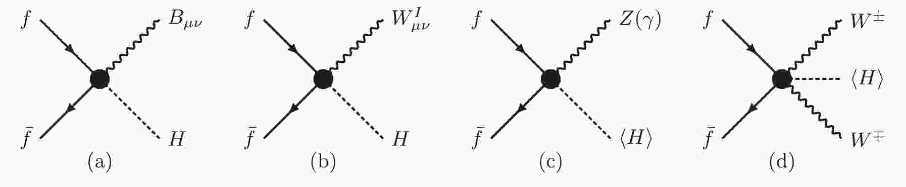
$ L_i $ and$ Q_i $ denote the left-handed weak doublet of the i-th generation in the SM, and$ e_i (u_i, d_i) $ the right-handed weak singlet of charged leptons (up-type and down-type quarks), respectively. Figure 1(a) and 1(b) show Feynman diagrams of the dimension-6 operators. After spontaneously breaking symmetry, the operator yields$ f\bar{f}V $ and$ f\bar{f}VV $ anomalous couplings; see (c) and (d). The$ f\bar{f}V $ anomalous couplings give rise to the magnetic moment ($ a_\gamma^f $ ) and weak magnetic moment ($ a_W^f $ ) of the fermion f as follows:
Figure 1. Feynman diagrams of dimension-6 operators before (a, b) and after electroweak symmetry breaking (c, d).
$ \begin{aligned}[b] \delta a_\gamma^{f = u,c,t} =& -2 \sqrt{2} \frac{m_f v}{\Lambda^2} \frac{1}{e Q_f} (c_W\; C_{fB}+s_W\; C_{fW}) ,\\ \delta a_W^{f = u,c,t} =& +2 \sqrt{2} \frac{m_f v}{\Lambda^2} \frac{1}{e Q_f} (s_W\; C_{fB}-c_W\; C_{fW}) ,\\ \delta a_\gamma^{f = \ell,d,s,b} =& -2 \sqrt{2} \frac{m_f v}{\Lambda^2} \frac{1}{e Q_f} (c_W\; C_{fB}-s_W\; C_{fW}) ,\\ \delta a_W^{f = \ell,d,s,b} =& +2 \sqrt{2} \frac{m_f v}{\Lambda^2} \frac{1}{e Q_f} (s_W\; C_{fB}+c_W\; C_{fW}), \end{aligned} $

(3) where
$ Q_f $ and$ m_f $ denote the charge and mass of the fermion f, respectively.$ v = 246\; {\rm GeV} $ is the vacuum expectation value of the Higgs doublet after symmetry breaking, and$ s_W $ and$ c_W $ denote sine and cosine of the Weinberg angle, respectively. As$ a_\gamma^f $ and$ a_W^f $ are orthogonal in the parameter space of$ C_{fB} $ and$ C_{fW} $ , one has to measure both$ a_\gamma^f $ and$ a_W^f $ to probe the NP effects.The magnetic moments of up-quarks and down-quarks
$ a_\gamma^{u,d} $ and$ a_W^{u,d} $ (corresponding to the operators$ O_{uW/dW} $ and$ O_{uB/dB} $ ) are tightly constrained through Drell-Yan processes,$ VV $ pair production, and$ VH $ associated production at the LHC [7, 8]. The operators$ O_{tW} $ and$ O_{tB} $ of top quarks can be examined in single-top productions or top-quark decays [9-13].$ a_W^{s,c,b} $ is bounded by the precise measurements at the LEP [14-17], which yield$ \begin{aligned}[b] & \Big| s_W C_{s(b) B} + c_W C_{s(b) W}\Big|\left(\frac{1\; \text{TeV}}{\Lambda}\right)^2 \leqslant 4.2, \\& \Big| s_W C_{c B} - c_W C_{c W}\Big| \left(\frac{1\; \text{TeV}}{\Lambda}\right)^2\leqslant 4.2\; . \end{aligned} $

(4) In this work, we show that
$ a_\gamma^{s,c,b} $ induced by the two operators can be tested in the process of$ pp\to H \gamma $ at the LHC with an integrated luminosity of$ 3000\; {\rm fb}^{-1} $ (HL-LHC).One cannot separate the Wilson coefficients
$ C_i $ 's and the NP scale$ \Lambda $ when evaluating the contributions of dimension-6 operators in physical observables. Therefore, we choose$ 1\; {\rm TeV} $ as a reference of NP scale$ \Lambda $ to obtain dimensionless constraints of the magnetic moment operators. A general choice of scale$ \Lambda $ can be obtained from our results.The magnetic moments of electrons and muons are severely constrained by the Z-boson width measurement at the LEP [17] and the measurements of the magnetic moment [18-25]; therefore, we do not consider the electron or muon in this work. The LEP constraint on
$ a_W^\tau $ of the$ \tau $ -lepton reads as [14-17, 26, 27]$ \Big| s_W C_{\tau B} + c_W C_{\tau W}\Big|\left(\frac{1\; \text{TeV}}{\Lambda}\right)^2 \leqslant 0.28 \; , $

(5) while the constraint on
$ a_\gamma^\tau $ is$ -12.8 \leqslant \big(c_W C_{\tau B} - s_W C_{\tau W}\big) \left(\frac{1\; \text{TeV}}{\Lambda}\right)^2 \leqslant 3.2 \; . $

(6) We demonstrate that
$ a_\gamma^\tau $ can be measured in the process of$ gg \to H \to \tau^+ \tau^- \gamma $ at the HL-LHC. -
In this section, we examine the effects of magnetic-moment operators in the
$ pp\to H \gamma $ process at the HL-LHC, which has been studied extensively in the literature [28-32]. We consider one flavor at a time throughout this work. Figure 2(a) and (b, c) display Feynman diagrams of the$ H\gamma $ production induced by the operators$ O_{fB} $ and$ O_{fW} $ . The SM process is shown in Fig. 2(d, e). There are non-zero interference effects between the operator-induced diagrams and the SM diagrams. Therefore, we also treat the interference effect as the signal. However, as explained below, only the first diagram contributes after applying hard kinematic cuts, and the interference effects are negligible.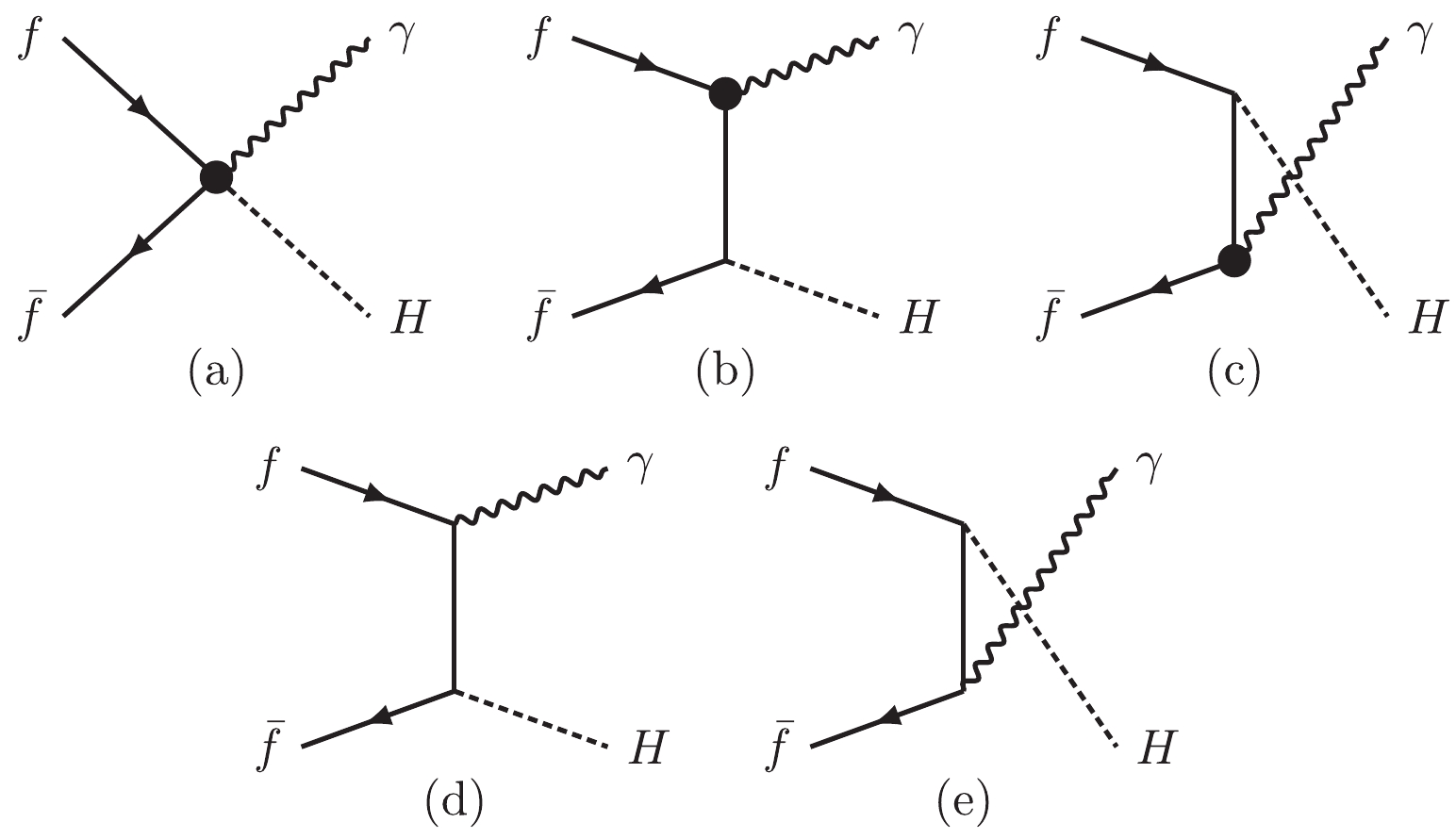
Figure 2. Feynman diagrams of
$ H \gamma $ production.In our simulation, the Higgs bosons are required to decay into a pair of bottom quarks. This is the predominant decay mode of the Higgs boson. The event topology of the signal process is two bottom quarks plus a photon. The SM backgrounds are
$ \begin{aligned}[b] & pp\to \gamma +\text{jets},\\ & pp\to t \bar{t} \gamma,\\ & pp\to Z \gamma ,\\ & pp\to t\gamma/\bar{t}\gamma +\text{jets}, \end{aligned} $

(7) with the Z boson and top quark hadronic decay. It is noted that background
$ \gamma+\text{jets} $ consist of$ \gamma+b\bar{b} $ ,$ \gamma+c\bar{c} $ ,$ \gamma\; + $ light flavor jets and etc.We generate signal and background events utilizing MadEvent [33] and pass those to Pythia [34] and Delphes [35] for parton showering, hadronization, and collider simulation. Both the renormalization and factorization scales are chosen as the dynamics scale
$ \mu_0 $ , defined as the scalar sum of the transverse momentum of the final state objects. In order to avoid collinear and soft divergences in the process of$ pp\to \gamma+\text{jets} $ , we apply the kinematic cuts at the generator level as follows:$ \begin{aligned}[b] & p_\text{T}^\gamma\geqslant 30\; \mathrm{GeV}, \; \;\;|\eta_{\gamma}|\leqslant 2.5, \\& p_\text{T}^j\geqslant 30\; \mathrm{GeV}, \; \;\;|\eta_{j}|\leqslant 2.5, \\ & \Delta R_{jj}>0.4,\; \;\;\Delta R_{j\gamma}> 0.4, \end{aligned} $

(8) where
$ p_{\rm T}^{\gamma/j} $ and$ \eta^{\gamma/j} $ are the transverse momentum and pseudo-rapidity of$ \gamma $ and jet, respectively, and$ \Delta R_{ij}\equiv $ $ \sqrt{(\phi_{i} - \phi_{j})^2 + (\eta_{i}-\eta_{j})^2} $ is the angular distance between objects i and j in the azimuthal angle ($ \phi $ )-pseudurapidity ($ \eta $ ) plane. At the detector level, two b-jets are required in the final state to suppress the SM backgrounds. In the simulation, we utilize b-tagging technology [36, 37] to distinguish the jet flavor. The b-tagging efficiency is chosen as 70%, the mistagging rate of c-quarks and light flavor quarks is 10% and 1%, respectively. We require at least one photon in the final state, i.e.,$ n^{b-\rm{jet}} = 2,\; n^\gamma \geqslant 1. $

(9) Figure 3 displays the normalized distributions of
$ p_{\text T}^\gamma $ (a),$ \eta^\gamma $ (b),$ M_{b\bar{b}} $ (c), and$ M_{b\bar{b}\gamma} $ (d) after imposing the basic cuts given in Eq. (8) and Eq. (9). For demonstration, we plot the distributions of the signal events induced by operators$ O_{cB} $ and$ O_{bB} $ , respectively. This shows that the photons in the signal events exhibit a hard$ p_{\text T} $ and mainly appear in the central region of the detector; see the black-solid and the red-solid curves. The reason can be understood as follows. In the signal events, the two fermions in the initial state are in different chirality states and thus are in the s-wave state. In order to respect the angular momentum conservation, the particles in the final state are in the p-wave state such that the matrix element is proportional to$ p_{\rm T}^\gamma $ . As a result, the matrix element of the signal process is proportional to$ \sin\theta $ , where$ \theta $ is the polar angle of the photon with respect to the beam line in the center of mass frame. On the other hand, the photons in the background mainly arise from the QED radiation and tend to be soft.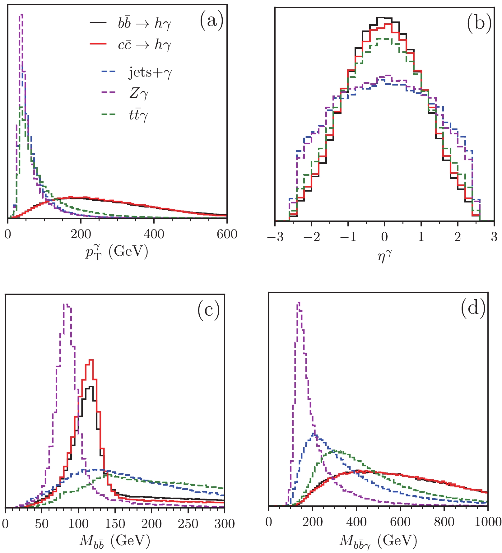
Figure 3. (color online) Normalized distributions of
$ p_{\text{T}}^\gamma $ (a),$ \eta^\gamma $ (b),$ M_{b\bar b} $ (c), and$ M_{b\bar b\gamma} $ (d). Black (red) solid curve denotes distributions of signal events induced by operator$ O_{bB} $ ($ O_{cB} $ ), respectively. Operator$ O_{bW} $ ($ O_{cW} $ ) yields exactly same normalized distributions as operator$ O_{bB} $ ($ O_{cB} $ ), respectively. Dashed curves indicate SM backgrounds from$ \gamma+{\rm jets} $ (blue),$ Z\gamma $ (magenta), and$ t \bar{t}\gamma $ (green), respectively.For illustration, we present the leading contributions of the squared matrix elements of the
$ f\bar{f}\to H\gamma $ process:$ \begin{aligned}[b] |M_{a}|^2 =& \frac{2N_c (c_W\; C_{fB}\pm s_W\; C_{fW})^2 (s-m_H^2)^2}{\Lambda^4}\sin^2\theta, \\ |M_{b}+M_{c}|^2 =& \frac{16N_c (c_W\; C_{fB}\pm s_W\; C_{fW})^2 m_f^2s}{\Lambda^4}, \\ |M_{d}+M_{e}|^2 =& \frac{16 N_c Q_f^2 e^2 m_f^2 ( s^2 + m_H^4 ) }{ v^2 (s-m_H)^2 \sin^2\theta}, \\ {\rm Re}(M^\dagger_{a}(M_{d}+M_{e})) =& \frac{4\sqrt{2} N_c Q_f e m_f m_H^2 (c_W\; C_{fB}\pm s_W\; C_{fW}) }{\Lambda^2 v}, \end{aligned} $

(10) where
$ N_c = 3 $ is the color factor, and$ \sqrt{s} $ is the collision energy. The subscript of the matrix element denotes the corresponding Feynman diagram in Fig. 2. In the region of large colliding energy, only$ |M_{a}|^2 $ contributes, while the others' contributions are negligible. Indeed,$ |M_{a}|^2 $ is proportional to$ \sin^2\theta $ .Taking advantage of the hard photon in the signal events, we impose a hard
$ p_{\rm T} $ cut on the photon with the largest$ p_{\rm T} $ as follows:$ p_\text{T}^\gamma\geqslant 300\; \mathrm{GeV}, $

(11) to suppress the SM backgrounds.
Figure 3(c) displays the normalized distributions of the invariant mass of two b-jets (
$ M_{b \bar{b} } $ ). The two b-jets in the signal event originate from the Higgs boson decay; therefore, their invariant mass is around$ m_H $ ; see the black-solid and the red-solid curves. Similarly, there is a peak around$ m_Z $ in the$ Z \gamma $ backgrounds. The two b-jets in other SM backgrounds are not from a resonance decay and yield a flat$ M_{b \bar{b} } $ distribution. We impose a mass window cut on the two b-jets,$ \left|M_{b \bar{b} }-m_H\right| \leqslant 15\; \mathrm{GeV}, $

(12) to suppress the SM backgrounds.
Figure 3(d) displays the normalized distributions of the invariant mass of two b-jets and a photon (
$ M_{ b \bar{b} \gamma} $ ). The signal events tend to have a large invariant mass, while the background events prefer the small invariant mass region. In order to suppress the SM backgrounds, we further impose a hard cut on$ M_{ b \bar{b} \gamma} $ as following:$ M_{ b \bar{b} \gamma} \geqslant 700\; \mathrm{GeV}. $

(13) Table 1 lists the numbers of the signal events and background events after the basic cuts and optimal cuts (i.e.,
$ p_{\text T}^\gamma $ ,$ M_{b\bar{b}} $ , and$ M_{b\bar{b}\gamma} $ cuts) at the HL-LHC. Note that the NP scale$ \Lambda $ is set to be$ 1\; {\rm TeV} $ . The major SM background comes from the$ \gamma+{\rm jets} $ process in which the$ \gamma b\bar{b} $ channel dominates. As both the$ O_{fB} $ and$ O_{fW} $ operators contribute to the signal process through the same$ f\bar{f}VH $ vertex, they generate the same differential distributions and therefore have the same cut efficiencies. The$ O_{fW} $ and$ O_{fB} $ operators differ in the cross section by a total factor$ \tan^2\theta_W $ .Signal processes Basic cuts Optimal cuts $ C_{bB}=1 $ ,

$ C_{bW}=0 $ 

$ 9.38\times 10^{3} $ 

$ 815 $ 

$ C_{bB}=0 $ ,

$ C_{bW}=1 $ 

$ 2.82\times 10^{3} $ 

$ 245 $ 

$ C_{cB}=1 $ ,

$ C_{cW}=0 $ 

$ 2.78\times 10^{4} $ 

$ 3.17\times 10^{3} $ 

$ C_{cB}=0 $ ,

$ C_{cW}=1 $ 

$ 8.37\times 10^{3} $ 

$ 953 $ 

$ C_{sB}=1 $ ,

$ C_{sW}=0 $ 

$ 3.86\times 10^{4} $ 

$ 4.79\times 10^{3} $ 

$ C_{sB}=0 $ ,

$ C_{sW}=1 $ 

$ 1.16\times 10^{4} $ 

$ 1.44\times 10^{3} $ 

Background processes Basic Cuts Optimal cuts $ \gamma $ +jets

$ 3.32 \times 10^{8} $ 

$ 9.90\times 10^{4} $ 

$ Z\gamma $ 

$ 5.80 \times 10^{5} $ 

$ 828 $ 

$ t\bar{t}\gamma $ 

$ 4.85 \times 10^{5} $ 

$ 1.25\times 10^{3} $ 

$ t\gamma/\bar{t}\gamma +\text{jets} $ 

$ 2.40 \times 10^{5} $ 

$ 106 $ 

Table 1. Number of signal and background events at HL-LHC for
$\Lambda = 1\; {\rm TeV}.$ Equipped with the optimal cuts shown above, we vary the Wilson coefficients to obtain a 5 standard deviation (
$ \sigma $ ) statistical significance using$ \sqrt{-2\left[(n_b + n_s) \log\frac{n_b}{n_s+n_b}+n_s\right]} = 5, $

(14) where
$ n_b $ and$ n_s $ represent the numbers of the signal and background events, respectively. The number of signal events in Table 1 is calculated with the choice of$ C_{fW} = 1 $ or$ C_{fB} = 1 $ ($ f = c,s,b $ ), and$ \Lambda = 1\; {\rm TeV} $ . Denote the number of the signal events in the last column of Table 1 after all cuts as$ n_s^0 $ .$ n_s^f $ for a general choice of$ C_{fW} $ ,$ O_{fB} $ , and$ \Lambda $ can be obtained as follows:$ \begin{aligned}[b] n_s^s =& n_s^0\Big|_{C_{sB} = 1}\times\frac{(c_W C_{sB} - s_W C_{sW})^2}{c_W^2} \left(\frac{1\; \text{TeV}}{\Lambda}\right)^4 , \\ n_s^c =& n_s^0\Big|_{C_{cB} = 1}\times \frac{(c_W C_{cB} + s_W C_{cW})^2}{c_W^2} \left(\frac{1\; \text{TeV}}{\Lambda}\right)^4 , \\ n_s^b =& n_s^0\Big|_{C_{bB} = 1}\times\frac{(c_W C_{bB} - s_W C_{bW})^2}{c_W^2} \left(\frac{1\; \text{TeV}}{\Lambda}\right)^4. \end{aligned} $

(15) Using Eq. (14), we determine that a
$ 5\sigma $ discovery significance requires$ \begin{aligned}[b] & \Big|c_W C_{sB} - s_W C_{sW}\Big|\left(\frac{1\; \text{TeV}}{\Lambda}\right)^2\geqslant 0.506^{+0.006}_{-0.004},\\ & \Big|c_W C_{cB} + s_W C_{cW}\Big|\left(\frac{1\; \text{TeV}}{\Lambda}\right)^2\geqslant 0.622^{+0.016}_{-0.009},\\& \Big|c_W C_{bB} - s_W C_{bW}\Big|\left(\frac{1\; \text{TeV}}{\Lambda}\right)^2\geqslant 1.228^{+0.070}_{-0.053}\; , \end{aligned} $

(16) where the superscripts and subscripts shows the results of the choices of the renormalization and factorization scales as
$ \mu_0/2 $ and$ 2\mu_0 $ , respectively.Figure 4 displays the
$ 5\sigma $ discovery region in the plane of$ C_{f W} $ and$ C_{f B} $ for the strange-quark (a), charm-quark (c), and bottom-quark (c) in the$ H\gamma $ production at the HL-LHC (yellow-meshed band). The yellow bound denotes the allowed$ 2\sigma $ parameter space by the Z-boson width measurement at the LEP. We consider one flavor at a time. The HL-LHC has a great potential of probing$ O_{s(c,b)B} $ and$ O_{s(c,b)W} $ in comparison with the LEP. The operator$ O_{bW} $ is highly constrained by the$ b\to s\gamma $ measurement [11, 12], i.e.,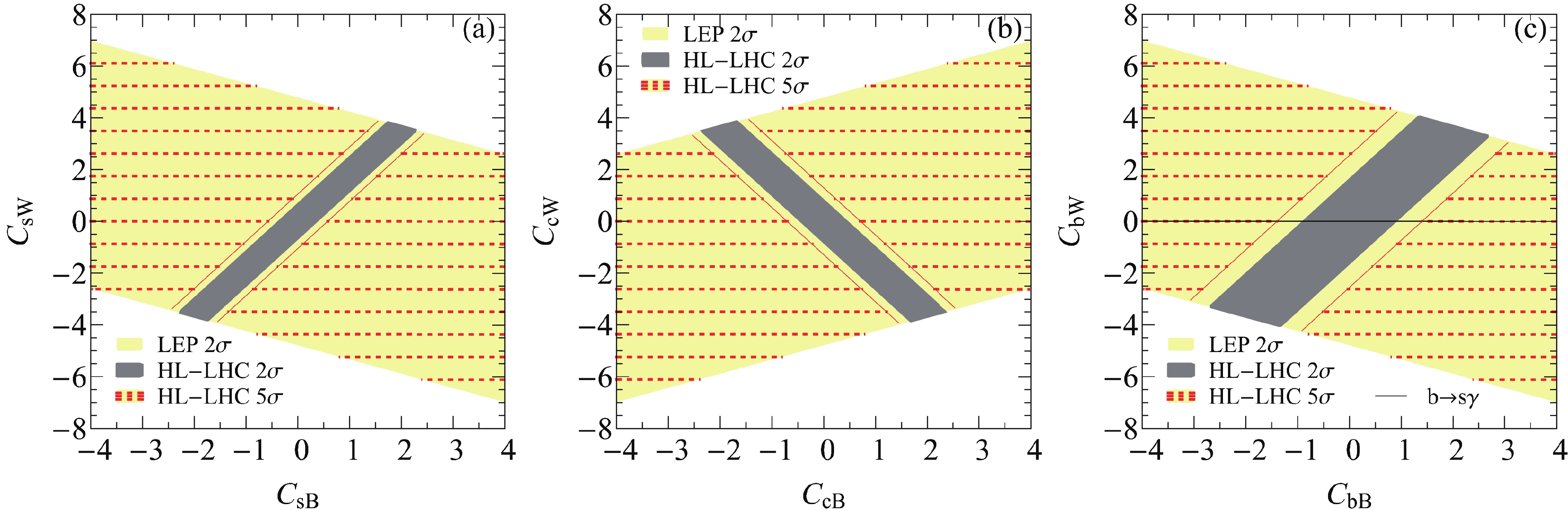
Figure 4. (color online) Yellow-meshed bands denote
$ 5\sigma $ discovery region of$ C_{fB} $ and$ C_{fW} $ for s-quark (a), c-quark (b), and b-quark (c) in$ H\gamma $ production with$ \Lambda = 1\; {\rm TeV} $ at HL-LHC, respectively, while yellow bounds denote allowed regions by$ 2\sigma $ bounds at LEP. Gray band denotes allowed region at$ 2\sigma $ significance if no NP effects are observed in$ H\gamma $ production. Black line in (c) denotes$ 2\sigma $ constraint of$ b\to s\gamma $ measurement.$ -0.008 \leqslant C_{bW}\leqslant 0.011\; .$

(17) We plot the constraint of
$ b\to s\gamma $ on$ O_{bW} $ at a 95% confidence level in Fig. 4(c); see the black line. Obviously, the constraints from the$ b\to s\gamma $ measurement are much more stringent; however, these can constrain$ O_{bW} $ but not$ O_{bB} $ .If no deviation is observed in the
$ H\gamma $ production, then we can set an upper limit on the Wilson coefficients at the$ 2\sigma $ confidence level in terms of$ \sqrt{-2 \left(n_b \ln \frac{n_s + n_b}{n_b}-n_s \right)} = 2.0, $

(18) which yields bounds on the Wilson coefficients at the 95% confidence level as follows:
$ \begin{aligned}[b]& \Big|c_W C_{sB} - s_W C_{sW}\Big|\left(\frac{1\; \text{TeV}}{\Lambda}\right)^2\leqslant 0.320^{+0.004}_{-0.003},\\ & \Big|c_W C_{cB} + s_W C_{cW}\Big|\left(\frac{1\; \text{TeV}}{\Lambda}\right)^2\leqslant 0.394^{+0.009}_{-0.006},\\ & \Big|c_W C_{bB} - s_W C_{bW}\Big|\left(\frac{1\; \text{TeV}}{\Lambda}\right)^2\leqslant 0.776^{+0.045}_{-0.033}, \end{aligned} $

(19) see the gray bands in Fig. 4. The slope of the gray bands is
$ -\cot\theta_W $ for the up-type quarks and$ +\cot\theta_W $ for the down-type quarks. The gray bands are perpendicular to the yellow bounds owing to the mixing of the weak and hypercharge fields; see Eq. (3). -
The potential to detect the magnetic momentum of the
$ \tau $ lepton has been discussed for future lepton colliders [38]. In this section, we explore the HL-LHC potential of searching for$ O_{\tau B} $ and$ O_{\tau W} $ through the rare decay of$ H \to \tau^+\tau^-\gamma $ in the single Higgs-boson production process of$ gg\to H $ . There are two final$ \tau $ leptons. The case when one final$ \tau $ lepton decays in the leptonic mode and the other in the hadronic mode has been discussed [39]. In this paper, we explore the case when the two$ \tau $ leptons decay into the hadronic modes.The partial decay width of
$ H\to \tau^+\tau^-\gamma $ in the SM is tiny at$ \sim 8.68\times 10^{-6}\; \rm{GeV} $ [40] in comparison with the full width of the Higgs boson at$ \sim 4\; {\rm MeV} $ [41]. Table 2 shows the partial decay width and the branching ratio of the rare decay of$ H\to \tau^+\tau^-\gamma $ induced by operators$ O_{\tau B} $ and$ O_{\tau W} $ after the cut of$ p_{\text T}^\gamma\geqslant 10\; {\rm GeV} $ , which is used to trigger the signal event and suppress the SM backgrounds. To be more specific, we present the interference effect and the pure NP contribution (square) separately. The NP operator effects are comparable to the SM contribution.Operators Processes Width/GeV BR $ O_{\tau B} $ 

Interference $ 2.51 \times 10^{-6} $ 

$ 6.27 \times 10^{-4} $ 

Square $ 9.71 \times 10^{-7} $ 

$ 2.43 \times 10^{-4} $ 

$ O_{\tau W} $ 

Interference $ -1.35 \times 10^{-6} $ 

$ -3.38 \times 10^{-4} $ 

Square $ 2.81 \times 10^{-7} $ 

$ 7.04 \times 10^{-5} $ 

SM $ H\to \tau^\pm\tau^{\mp *}\to \tau^+\tau^-\gamma $ 

$ 8.68 \times 10^{-6} $ 

$ 2.17 \times 10^{-3} $ 

Table 2. Decay width and branching ratio of
$ H \to \tau^+ \tau^- \gamma $ with choice of$ C_{\tau B} = 1 $ or$ C_{\tau W} = 1 $ for$ \Lambda = 1\; {\rm TeV} $ after demanding$ p_{\text{T}}^\gamma \geqslant 10\; {\rm GeV} $ . SM contribution, pure NP contribution (square), and interference between SM and NP effects are listed separately.In the collider simulation, we require that the
$ \tau^\pm $ -leptons decay hadronically; therefore, the signal process of$ pp \to H \to \tau^+\tau^-\gamma $ yields a collider signature of two$ \tau $ -jets plus a hard photon. Figure 5 displays representative Feynman diagrams for the signal and background processes. The irreduciable backgrounds in the SM are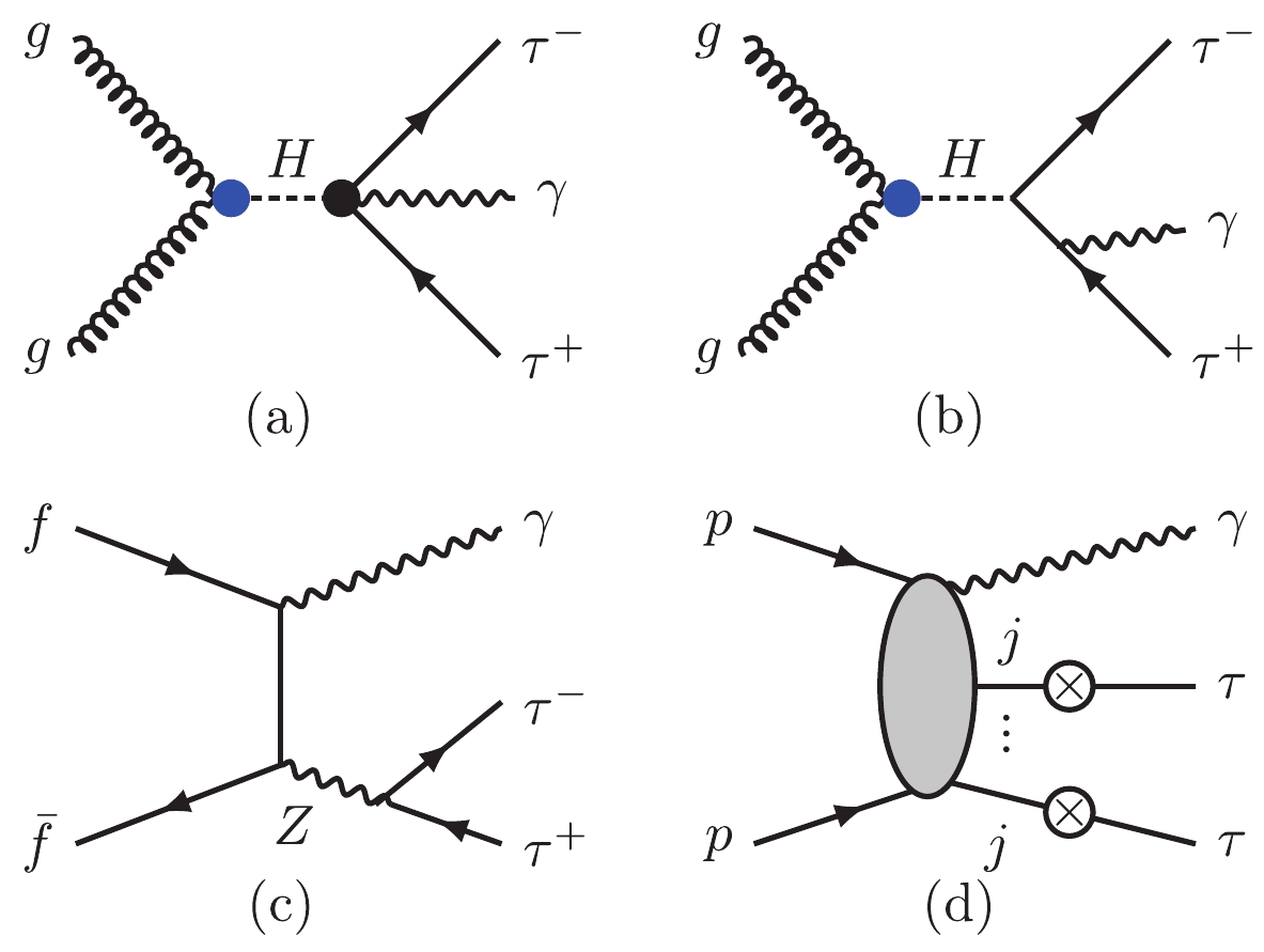
Figure 5. (color online) Feynman diagrams of signal process of
$ gg\to H \to \tau^+ \tau^- \gamma $ (a) and representative diagrams of SM backgrounds (b, c, d).$ \begin{aligned}[b] & pp\to Z\gamma\to\tau^+\tau^-\gamma,\\ & pp\to H\to\tau^+\tau^-\gamma, \end{aligned} $

(20) and the reducible QCD backgrounds are
$ pp\to \gamma+\text{jets}, $

(21) when at least two of the QCD jets are mistagged as
$ \tau $ -jets. The jet in the event is reconstructed using an anti-$ k_{\text{T}} $ jet algorithm [42] with$ R = 0.4 $ . The$ \tau $ -tagging efficiency of the hadronic decay$ \tau^\pm $ is chosen to be 60% with the mis-tagging rate$ \epsilon(j\to\tau) = 1\% $ .To tigger the signal event, we require a set of basic cuts as follows:
$ \begin{aligned}[b]& p_{\text T}^\gamma\geqslant 10\; {\rm GeV},\;\;\;\; |\eta_{\gamma}|\leqslant 2.5, \\& p_{\text T}^j\geqslant 20\; {\rm GeV}, \;\;\;\; |\eta_{j}|\leqslant 2.5, \\ &\Delta R_{\gamma j/ jj}\geqslant 0.4\; . \end{aligned} $

(22) Denote
$ j_1 $ as the$ \tau $ -jet with a larger$ p_\text{T} $ . Figure 6 displays the normalized distributions of$ p_{\text T}^\gamma $ (a),$ p_{\text T}^{j_1} $ (b) and$ M_{\tau^+ \tau^- \gamma} $ (c). In the signal event, the photon exhibits a$ p_{\text T} $ distribution harder than the$ \tau $ -jet. On the other hand, the photons in the background processes tend to be soft as they arise predominantly from the radiation of the charged leptons. In order to further suppress the SM backgrounds, we demand hard cuts on the$ p_{\text T} $ of the photons and$ \tau $ -jets as follows: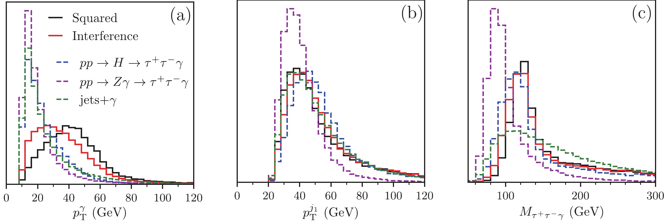
Figure 6. (color online) Normalized distributions of
$ p_{\text{T}}^\gamma $ (a),$ p_{\text T}^{j1} $ (b), and invariant mass$ M_{\tau^+ \tau^- \gamma} $ (c) after basic cuts given in Eq. (22). Sold black and solid red curves denote pure NP contribution (squared) and interference effect (interference) in signal event, respectively. Blue-dashed, magenta-dashed, and the green-dashed curves represent SM background processes.$ p_{\text T}^\gamma\geqslant 30\; \mathrm{GeV}, \; \; p_{\text T}^j\geqslant 30\; \mathrm{GeV}. $

(23) Figure 6(c) shows the normalized distributions of the invariant mass
$ M_{\tau^+ \tau^- \gamma} $ in which the signal process peaks around$ m_H $ and one of the background processes of$ pp \to Z \gamma $ peaks around$ m_Z $ . The$ \tau $ -jets in the QCD background mainly arise from the faked$ \tau $ -tagging and do not exhibit any resonance effect. Therefore, we require$ \left|M_{\tau^+ \tau^- \gamma}-m_H\right| \leqslant 15\; \mathrm{GeV} $

(24) to suppress the SM background from the process of
$ pp\to Z\gamma $ .Table 3 lists the numbers of the signal and the background events at the HL-LHC after the hard cuts and the mass window cut of
$ M_{\tau^+\tau^-\gamma} $ . We separate the signal contribution into the pure NP effect (square) and the interference effect. Again,$ O_{\tau B} $ and$ O_{\tau W} $ yield exactly the same cut efficiencies. As a result, the number of signal events for a general choice of$ C_{\tau B} $ and$ C_{\tau W} $ can be expressed as follows:Operators Process Hard cuts $ M_{\tau^+ \tau^- \gamma} $ 

$ C_{\tau B}=1 $ ,

$ C_{\tau W}=0 $ 

Interference $ 1.16\times 10^{3} $ 

$ 331 $ 

Square $ 470 $ 

$ 139 $ 

$ C_{\tau B}=0 $ ,

$ C_{\tau W}=1 $ 

Interference $ -624 $ 

$ -178 $ 

Square $ 136 $ 

$ 40.2 $ 

Backgrounds $ pp\to H \to \tau^+ \tau^- \gamma $ 

$ 5.75\times 10^{3} $ 

$ 1.63\times 10^{3} $ 

$ pp\to Z\gamma\to \tau^+ \tau^- \gamma $ 

$ 4.40\times 10^{4} $ 

$ 1.01 \times 10^{4} $ 

$ pp\to \gamma + $ jets

$ 8.11 \times 10^{6} $ 

$ 1.85 \times 10^{5} $ 

Table 3. Numbers of signal and background events after hard cuts and
$ M_{\tau^+\tau^-\gamma} $ mass window cut at HL-LHC for$\Lambda = 1\; {\rm TeV}.$ $ \begin{aligned}[b] n_s =& n_s^{\text{sqr}}\times\frac{(c_W C_{\tau B} - s_W C_{\tau W})^2}{c_W^2} \left(\frac{1\; \text{TeV}}{\Lambda}\right)^4 \\ &+n_s^{\text{int}}\times\frac{(c_W C_{\tau B} - s_W C_{\tau W})}{c_W} \left(\frac{1\; \text{TeV}}{\Lambda}\right)^2, \end{aligned} $

(25) where
$ n_s^{\text{sqr}} $ is the signal event number from the pure NP contribution (square), and$ n_s^{\text{int}} $ is the signal event number from the interference effect (interference) for$ C_{\tau B} = 1 $ and$ C_{\tau W} = 0 $ .Using Eq. (14), we determine that a
$ 5\sigma $ discovery significance in the process of$ gg\to H\to \tau^+\tau^-\gamma $ requires$ \begin{aligned}[b] \Big(c_W C_{\tau B} - s_W C_{\tau W}\Big)\left(\frac{1\; \text{TeV}}{\Lambda}\right)^2 \leqslant -4.73, \end{aligned} $

(26) or
$ \begin{aligned}[b] \Big(c_W C_{\tau B} - s_W C_{\tau W}\Big)\left(\frac{1\; \text{TeV}}{\Lambda}\right)^2 \geqslant 2.62\; . \end{aligned} $

(27) Figure 7 shows the parameter space of
$ 5\sigma $ discovery in the plane of$ C_{\tau B} $ and$ C_{\tau W} $ obtained from the process of$ gg\to H\to \tau^+\tau^-\gamma $ at the HL-LHC (yellow-meshed band) with$ \Lambda = 1\; {\rm TeV} $ . The yellow bound denotes the$ 2\sigma $ parameter space allowed by the LEP measurement [17]. The HL-LHC can cover the most of the parameter space that cannot be accessed at the LEP.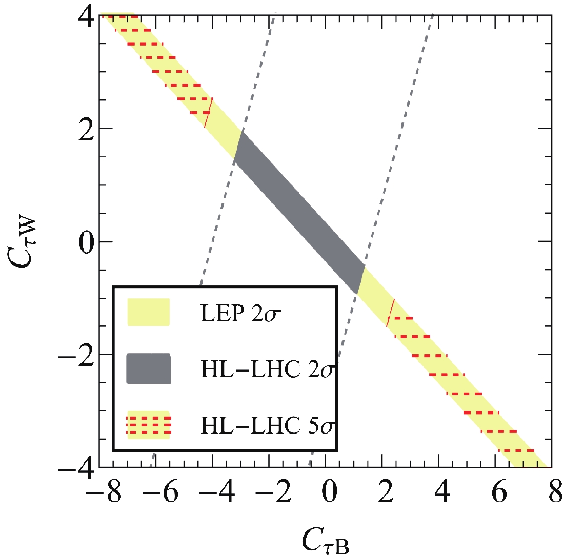
Figure 7. (color online) Yellow-meshed bands denote
$ 5\sigma $ discovery region of$ C_{\tau B} $ and$ C_{\tau W} $ in process of$ gg\to H\to \tau^+\tau^-\gamma $ at HL-LHC with$ \Lambda = 1\; {\rm TeV} $ . Yellow bounds denote$ 2\sigma $ parameter space allowed by Z-pole measurement at LEP. Region between two dashed lines is allowed at$ 2\sigma $ significance if no NP effects are observed at HL-LHC, where overlapped gray band satisfies both LEP and HL-LHC bounds.If no deviation is found in the process of
$ gg\to H\to \tau^+\tau^-\gamma $ , then we obtain a bound on the Wilson coefficients at the 95% confidence level as$ -3.51 \leqslant \Big(c_W C_{\tau B} - s_W C_{\tau W}\Big)\left(\frac{1\; \text{TeV}}{\Lambda}\right)^2 \leqslant 1.41, $

(28) see the region between the two dashed lines. The overlapped gray band satisfies both the LEP and the HL-LHC bounds.
-
The magnetic moment and weak magnetic moment of SM fermions are sensitive to quantum effects of new physics resonances. For each fermion f there are two independent operators that generate the magnetic moment and weak magnetic moment:
$ O_{fB} $ involving the hypercharge field and$ O_{fW} $ involving the weak field. After symmetry breaking, the magnetic moment and the weak magnetic moment depend on the orthogonal combinations of the two operators. Therefore, at least two independent experiments are needed to probe$ O_{fB} $ and$ O_{fW} $ .The weak magnetic moment of the strange-quark (s), charm-quark (c), or bottom-quark (b) is bounded by the width measurement of the Z-boson at the LEP, but the magnetic moments of the three quarks are less constrained. In this paper, we explored the potential of the HL-LHC on probing the operators
$ O_{f B} $ and$ O_{f W} $ ($ f = s,c,b $ ) in the process of$ pp\to H\gamma $ , in which the magnetic moment of the quarks dominates. We consider one flavor of quarks at a time. We showed that in most of the parameter space that cannot be accessed at the LEP, a$ 5\sigma $ significance discovery can be reached in the$ H\gamma $ production at the HL-LHC.The magnetic moment and weak magnetic moment of the electron or muon have been accurately measured and thus severely constrained. In analogue to the electron and muon leptons, the weak magnetic moment of the
$ \tau $ lepton is also bounded at the LEP; however, the magnetic moment of the$ \tau $ lepton is less bounded. In this work, we considered the rare decay of$ H\to \tau^+\tau^-\gamma $ induced by$ O_{\tau B} $ and$ O_{\tau W} $ and examined the potential of probing the two operators in the process of$ gg\to H \to \tau^+\tau^-\gamma $ . Similar to the case of quark operators, in most of the parameter space that cannot be accessed at the LEP, a$ 5\sigma $ significance discovery can be reached in the process of$ gg\to H\to \tau^+\tau^-\gamma $ at the HL-LHC.In summary, one can probe the magnetic moment of the
$ s(c,b) $ quarks in the process of$ pp\to H\gamma $ and the magnetic moment of the$ \tau^\pm $ lepton in the$ gg\to H\to\tau^+\tau^-\gamma $ at the HL-LHC. -
In the simulation of the process of
$ pp\to H\gamma $ , we require a hard cut on the invariant mass of final state particles, namely,$ M_{b\bar{b}\gamma}>700 $ GeV, which corresponds to the collision energy of initial state quark pairs and is close to the benchmark NP scale$ \Lambda = 1\; {\rm TeV} $ . In the Appendix, we discuss the validity domain of these operators by using unitarity constraints, especially to validate the hard cuts used in our analysis.Considering the contributions of the magnetic moment operators in the process of
$ f\bar{f}\to H\gamma $ , the first process in Fig. 2(a) dominates as stated above. Therefore, we calculate the unitarity bound from the matrix element$ M_a $ following Refs. [43-46]. The high energy helicity amplitudes can be projected to partial wave amplitudes as follows:$\tag{A1} \begin{array}{l} M_a(\lambda_f,\lambda_{\bar{f}},\lambda_\gamma) = 16 \pi \displaystyle\sum_J (2J+1) {\rm e}^{{\rm i}(\lambda-\kappa)\phi}d^J_{\lambda,\kappa}(\theta) a^J_{\lambda,\kappa}, \end{array} $

where
$ \lambda_{f (\bar{f}, \gamma)} $ is the helicity of the quark (anti-quark, photon), respectively. The$ a^J_{\lambda,\kappa} $ is the partial wave amplitude of the J wave, where$ \lambda = \lambda_f-\lambda_{\bar{f}} $ and$ \kappa = \lambda_\gamma $ . Utilizing the completeness relation of Wigner d-functions, the partial wave amplitude$ a^J_{\lambda,\kappa} $ is given by$\tag{A2} \begin{aligned} a^J_{\lambda,\kappa} = \frac{1}{32\pi}\int_{-1}^{1} {\rm d}\cos\theta d^J_{\lambda,\kappa}(\theta) M_a(\lambda_f,\lambda_{\bar{f}},\lambda_\gamma). \end{aligned} $

With the normalization
$ {\rm Im}(a^J_{\lambda,\kappa}) = |a^J_{\lambda,\kappa}|^2 $ , the unitarity condition for each partial wave reads$\tag{A3} |{\rm Re}(a_{\lambda,\kappa}^J)|<\frac{1}{2}.$

The non-zero helicity amplitudes of the process of
$ f\bar{f}\to H\gamma $ are$ \begin{aligned}[b] M_a \left(-\frac{1}{2},-\frac{1}{2},+1\right) = \frac{ (c_W\; C_{fB}\pm s_W\; C_{fW}) (s-m_H^2) \sin\theta}{\Lambda^2}, \end{aligned} $

$\tag{A4} \begin{aligned}[b] M_a \left(+\frac{1}{2},+\frac{1}{2},-1\right) = -\frac{ (c_W\; C_{fB}\pm s_W\; C_{fW}) (s-m_H^2) \sin\theta}{\Lambda^2}, \end{aligned} $

where
$ ``+" $ and$ ``-" $ on the right-hand side corresponds to up-type and down-type quarks, respectively. The 4-momenta of the four external particles are chosen as$\tag{A5} \begin{aligned}[b] p^f =& \frac{\sqrt{s}}{2}(1,0,0,1), \\ p^{\bar{f}} =& \frac{\sqrt{s}}{2}(1,0,0,-1), \\ p^\gamma =& \frac{s-m_H^2}{2\sqrt{s}}(1,\sin\theta,0,\cos\theta), \\ p^H =& \left(\frac{s+m_H^2}{2\sqrt{s}},-\frac{s-m_H^2}{2\sqrt{s}}\sin\theta,0,-\frac{s-m_H^2}{2\sqrt{s}}\cos\theta \right), \end{aligned} $

where
$ \sqrt{s} $ is the center-of-mass energy. With the helicity amplitudes, the$ J = 1 $ partial wave amplitudes are$\tag{A6} \begin{aligned} a_{0,1}^{J = 1} = a_{0,-1}^{J = 1} = \frac{(c_W\; C_{fB}\pm s_W\; C_{fW}) (s-m_H^2)}{24\sqrt{2}\pi\Lambda^2}, \end{aligned} $

from which one can obtain the unitarity bound on center-of-mass energy as follows:
$\tag{A7} s \lesssim \frac{12\sqrt{2}\pi\Lambda^2}{\Big| c_W\; C_{fB}\pm s_W\; C_{fW} \Big|}. $

We thus get the allowed range for the CM energies of the process of
$ f\bar{f}\to H\gamma $ such that they lie below the point where unitarity effects show up. This saturation energy is obviously of the order of$ \Lambda $ . For example,$ \sqrt{s}\lesssim 7.8\; \text{TeV} $ for$ C_{fB} = 1 $ ,$ C_{fW} = 0 $ , and$ \Lambda = 1\; {\rm TeV} $ ;$ \sqrt{s}\lesssim 10.5\; \text{TeV} $ for$ C_{fB} = 0 $ ,$ C_{fW} = 1 $ , and$ \Lambda = 1\; {\rm TeV} $ .The bounds on the CM energies from the unitarity requirement are much higher than
$ \Lambda $ , i.e., the effective field theory validates up to about 10 TeV even in the case of$ \Lambda = 1\; {\rm TeV} $ . At the 14 TeV LHC, the effective collision energy of the signal events cannot reach the unitarity bound of$ \sqrt{s} $ ; therefore, the hard cut of$ M_{b\bar{b}\gamma}>700 $ GeV does not violate the unitarity constraint.
Probing magnetic moment operators in ${\boldsymbol H \gamma }$ production and ${\boldsymbol H \to \tau^+ \tau^- \gamma }$ rare decay
- Received Date: 2021-06-08
- Available Online: 2021-09-15
Abstract: The magnetic moment (


 DownLoad: