


 Abstract
 HTML
HTML Reference
 Related
 PDF
PDF


-
At present, there are several interesting excesses in B-physics measurements involving the transition
$ b\to s\ell^+\ell^- $ ($ \ell = \mu, e $ )$ R_{K^{(*)}} \equiv \frac{B \to K^{(*)} \mu^+ \mu^-}{B \to K^{(*)} e^+ e^-}. $

(1) The LHCb results for the
$ R_K $ ratio in one$ q_2 $ bin [1, 2] and the$ R_{K^*} $ ratio in two$ q_2 $ bins [3] were found to lie significantly below one:$ \begin{aligned}[b] & R_K = 0.846^{+0.060}_{-0.054}\text{(stat)}^{+0.016}_{-0.014}\text{(syst)} \,,\\ & q^2 \in [1,6]\; \text{GeV}^2 \,, \\ &R_{K^\ast} = 0.660^{+0.110}_{-0.070}\text{(stat)}\pm 0.024\text{(syst)} \,, \\ &q^2 \in [0.045,1.1]\; \text{GeV}^2\,, \\ &R_{K^\ast} = 0.685^{+0.113}_{-0.069}\text{(stat)}\pm0.047\text{(syst)} \,, \\ &q^2 \in [1.1,6.0]\; \text{GeV}^2 \,. \end{aligned} $

(2) Belle announced its measurement of
$ R_{K^*} $ [4]:$ R_{K^*} = \begin{cases} 0.52^{+0.36}_{-0.26} \pm 0.05 \; ,\; \; 0.045 \leqslant q^2 \leqslant 1.1 \; {\rm GeV}^2 \; , \\ 0.96^{+0.45}_{-0.29} \pm 0.11 \; ,\; \; 1.1 \leqslant q^2 \leqslant 6.0 \; {\rm GeV}^2 \; , \\ 0.90^{+0.27}_{-0.21} \pm 0.10 \; ,\; \; 0.1 \leqslant q^2 \leqslant 8.0 \; {\rm GeV}^2 \; , \\ 1.18^{+0.52}_{-0.32} \pm 0.10 \; ,\; \; 15.0 \leqslant q^2 \leqslant 19.0 \; {\rm GeV}^2 \; , \\ 0.94^{+0.17}_{-0.14} \pm 0.08 \; ,\; \; 0.045 \leqslant q^2 \; . \end{cases} $

(3) Global fits to the experimental data show that a new physics model can explain the anomalies of
$ R(K) $ and$ R(K^{*}) $ by contributing to$ C_9^\mu $ . With$C_{10}^{\mu,\rm NP}$ = 0, the best fit value for$C_9^{\mu,\rm NP}$ is$ -1.10 \pm 0.16 $ [5].A
$ U(1)_{L_\mu-L_\tau} $ gauge boson couples only to$ \mu(\tau) $ but not to an electron [6], and this type of$ U(1)_{L_\mu-L_\tau} $ model has also been modified from its minimal version to explain the$ b \to s\mu^+\mu^- $ anomaly [7-23]. In Ref. [23], in addition to the$ U(1)_{L_\mu-L_\tau} $ gauge boson$ Z' $ and a complex singlet$ {\cal S} $ breaking$ U(1)_{L_\mu-L_\tau} $ symmetry, a vector-like$ SU(2)_L $ doublet quark Q and a complex singlet X are introduced to produce a$ Z'bs $ coupling large enough to explain the anomalies of$ R(K^{(*)}) $ . As the lightest component of X,$ X_I $ is a candidate of dark matter (DM). In this study, we combine the$ b\to s\mu^+\mu^- $ anomaly and DM experimental data to study the capability of the LHC to test dark matter,$ Z^{\prime} $ , and vector-like quarks.Our work is organized as follows. In Sec. II, we recapitulate the model. In Sec. III, we consider relevant theoretical constraints and
$ b\to s $ flavor observables and explain the$ b \to s\mu^+\mu^- $ anomaly. In Sec. IV, we discussDM observables. In Sec. V, we use the current searches at the LHC to constrain the parameter space and analyze the possibility of probing the new particles at the high luminosity LHC. Finally, we give our conclusion in Sec. VI. -
In addition to the
$ U(1)_{L_\mu-L_\tau} $ gauge boson$ Z' $ , the model predicts a complex singlet$ {\cal S} $ , a complex singlet X, and an$ SU(2)_L $ doublet quark Q. Their quantum numbers under the gauge group$ SU(3)_C\times SU(2)_L\times U(1)_Y\times U(1)_{L_\mu-L_\tau} $ are shown in Table 1.SU(3)c SU(2)L U(1)Y U(1) $ _{L_\mu-L_\tau} $ 

Q 3 2 $ +1/6 $ 

$ -q_x $ 

X 1 1 $ 0 $ 

$ q_x $ 

$ {\cal S} $ 

1 1 $ 0 $ 

$ -2q_x $ 

Table 1. Quantum numbers of the vector-like quark
$ Q\equiv(U,D) $ and scalars X and S under the gauge group$ SU(3)_C\times SU(2)_L\times U(1)_Y\times U(1)_{L_\mu-L_\tau} $ .The Lagrangian which remains invariant under the
$ SU(3)_C\times SU(2)_L\times U(1)_Y\times U(1)_{L_\mu-L_\tau} $ symmetry is given by$ \begin{aligned}[b] {\cal L} =& {\cal L}_{\rm SM} -{1 \over 4} Z'_{\mu\nu} Z^{\prime\mu\nu} + g_{Z'} Z'^{\mu}(\bar{\mu}\gamma_\mu \mu + \bar{\nu}_{\mu_L}\gamma_\mu\nu_{\mu_L} - \bar{\tau}\gamma_\mu \tau \\ &- \bar{\nu}_{\tau_L} \gamma_\mu\nu_{\tau_L})-V + \bar{Q} (i \not\!\! D -M_Q) Q+ (D_\mu X^\dagger) (D^\mu X)\\ & + (D_\mu {\cal S}^\dagger) (D^\mu {\cal S}) - \sum\limits_{i = 1}^3 (\lambda_i \bar{q}_L^i Q X + {\rm h.c.}). \end{aligned} $

(4) Here, we ignore the kinetic mixing term of gauge bosons of
$ U(1)_{L_\mu-L_\tau} $ and$ U(1)_Y $ .$ q^i_L $ denotes the SM left-handed quark doublet with$ i = 1,2,3 $ , and$ D_\mu $ is the covariant derivative. The field strength tensor is$ Z'_{\mu\nu} = \partial_\mu Z'_\nu- $ $ \partial_\nu Z'_\mu $ , and$ g_{Z'} $ is the gauge coupling constant of the$ U(1)_{L_\mu-L_\tau} $ group. The scalar potential V is given by$ \begin{aligned}[b] V = & -\mu_{h}^2 (H^{\dagger} H) - \mu_{S}^2 ({\cal S}^{\dagger} {\cal S}) + m_X^2 (X^{\dagger} X) + \left[\mu X^2 {\cal S} + \rm h.c.\right] \\ &+ \lambda_H (H^{\dagger} H)^2 + \lambda_S ({\cal S}^{\dagger} {\cal S})^2 + \lambda_X (X^{\dagger} X)^2 + \lambda_{SX} ({\cal S}^{\dagger} {\cal S})(X^{\dagger} X) \\ &+ \lambda_{HS}(H^{\dagger} H)({\cal S}^{\dagger} {\cal S}) + \lambda_{HX}(H^{\dagger} H)(X^{\dagger} X). \end{aligned} $

(5) The SM Higgs doublet H, the singlet filed
$ {\cal S} $ , and X are expressed as$ \begin{aligned}[b]&H = \left(\begin{array}{c} G^+ \\ \dfrac{1}{\sqrt{2}}\,(h_1+v_h+{\rm i}G) \end{array}\right)\,, {\cal S} = {1\over \sqrt{2}} \left( h_2+v_S+{\rm i}\omega\right) \,, \\ &X = {1\over \sqrt{2}} \left( X_R+{\rm i}X_I\right) \,, \end{aligned} $

(6) where
$ v_h = 246 $ GeV and$ v_S $ are, respectively, vacuum expectation values (VEVs) of H and$ {\cal S} $ , and the X field has no VEV. The mass parameters$ \mu^{2}_{h} $ and$ \mu^{2}_{S} $ in the potential of Eq. (5) are determined by the potential minimization conditions:$ \begin{aligned}[b] &\quad \mu_{h}^2 = \lambda_H v_h^2 + {1 \over 2} \lambda_{HS} v_S^2,\\ &\quad \mu_{S}^2 = \lambda_S v_S^2 + {1 \over 2} \lambda_{HS} v_h^2.\end{aligned} $

(7) After
$ {\cal S} $ acquires the VEV, the$ \mu $ term splits the complex scalar X into two real scalar fields$ X_R $ and$ X_I $ , and their masses are given by$ \begin{aligned}[b] &m_{X_R}^2 = m_X^2 + {1 \over 2} \lambda_{HX} v_H^2 + {1 \over 2}\lambda_{SX} v_S^2 + \sqrt{2} \mu v_S\\ &m_{X_I}^2 = m_X^2 + {1 \over 2} \lambda_{HX} v_H^2 + {1 \over 2}\lambda_{SX} v_S^2 - \sqrt{2} \mu v_S. \end{aligned} $

(8) The S field breaks the
$ U(1)_{L_\mu-L_\tau} $ symmetry spontaneously by developing a VEV. Since the X field does not develop a VEV, there is a remnant discrete$ Z_2 $ symmetry under which the X and Q fields are odd, and the other fields are even. Therefore, the lightest component$ X_I $ is stable and becomes a candidate of DM.The two physical CP-even states h and S are from the mixing of
$ h_1 $ and$ h_2 $ by the following relation:$ \begin{align} \left( \begin{array}{c} h_1 \\ h_2 \end{array} \right) = \left( \begin{array}{cc} \cos\theta & \sin\theta\\ -\sin\theta & \cos\theta \\ \end{array} \right) \left( \begin{array}{c} h \\ S \end{array} \right), \end{align} $

(9) where
$ \theta $ is the mixing angle. The two CP-even Higgses mediate the DM interactions:$ \begin{aligned}[b] {\cal L}(X_I X_I ,h,S) = & -{1 \over 2} \Big[\lambda_{HX} v_H c_\theta- (\lambda_{SX} v_S-\sqrt{2} \mu) s_\theta \Big] h X_I^2 \\ &-{1 \over 2} \Big[\lambda_{HX} v_H s_\theta + (\lambda_{SX} v_S-\sqrt{2} \mu) c_\theta \Big] S X_I^2. \end{aligned} $

(10) In this paper, in order to suppress the stringent constraints from direct and indirect DM detection experiments, we simply assume that the
$ hX_IX_I $ coupling is absent, namely taking$ \theta = 0 $ and$ \lambda_{HX} = 0 $ . For$ \theta = 0 $ , we obtain the following expressions:$ \lambda_{HS} = 0,\; \; \; \lambda_H = \frac{m_h^2}{2v_h^2},\; \; \; \lambda_S = \frac{m_S^2}{2v_S^2}. $

(11) After
$ {\cal S} $ obtains a VEV, the$ U(1)_{L_\mu-L_\tau} $ gauge boson$ Z' $ obtains a mass$ m_{Z'} = 2g_{Z'} \mid q_x\mid v_S. $

(12) The complex singlet X mediates the new Yukawa interactions of the vector-like quarks and the SM left-handed quark:
$ \ \Delta {\cal L}_{\rm Yukawa} = -{1 \over \sqrt{2}} \sum\limits_{i = 1,2,3} \left(\lambda_{u_i} \bar{u}_{iL} U +\lambda_{d_i} \bar{d}_{Li} D \right)(X_R +i X_I)+ {\rm h.c.}, $

(13) where we assume that the down-type quarks are already in the mass basis and rotate the interaction eigenstates of up-type quarks to the mass eigenstates via the CKM matrix V. Thus,
$ \lambda_{u_i} \equiv \sum\nolimits_j V_{ij} \lambda_j $ and$ \lambda_{d_i} \equiv \lambda_i $ with$ u_i = u,c,t $ and$ d_i = d,s,b $ . We simply set$ \lambda_1 = 0 $ to remove the constraints related to the first generation quarks. As a result,$ \lambda_u $ is much smaller than$ \lambda_c $ and$ \lambda_t $ due to the suppression of the factors of$ V_{us} $ and$ V_{ub} $ . -
In addition to
$ m_h = $ 125 GeV and$ v_h = $ 246 GeV, there are many new parameters in the model, and the input parameters taken in our calculations are shown in Table 2. We can determine other parameters from these input parameters, i.e.,$ v_S $ from Eq. (12),$ \lambda_H $ from Eq. (11),$ \lambda_S $ from Eq. (11),$ \mu $ and$ m_X^2 $ from Eq. (8), and$ \mu_h^2 $ and$ \mu_s^2 $ from Eq. (7).$ \; g_{Z'} $ 

$ q_x $ 

$ m_{Z'}\; $ 

$ \lambda_{HS}=0 $ 

$ \lambda_{HX}=0 $ 

$ \lambda_{SX}\; $ 

$ \lambda_X $ 

$ m_S $ 

$ m_{X_R} $ 

$ m_{X_I} $ 

$ m_Q $ 

$ \; \lambda_{b}\; $ 

$ \lambda_s\; $ 

Table 2. Input parameters in our calculations.
To maintain the perturbativity of the scalar potential, we conservatively take
$ \mid\lambda_{SX}\mid\leqslant 4\pi,\; \; \mid\lambda_X\mid\leqslant 4\pi. $

(14) The input mass parameters are scanned over the following ranges:
$ \begin{aligned}[b] & 60~ {\rm GeV} \leqslant m_{X_I} \leqslant 1~ {\rm TeV},\; \; \; 800~ {\rm GeV} \leqslant m_{X_R} \leqslant 2~ {\rm TeV},\\ &1~ {\rm TeV} \leqslant m_Q \leqslant 2~ {\rm TeV},\;\;\; 100~ {\rm GeV} \leqslant m_{Z'} \leqslant 1~ {\rm TeV}, \\ & 100~ {\rm GeV} \leqslant m_{S} \leqslant 1~ {\rm TeV}. \end{aligned} $

(15) Considering the bound of the neutrino trident process [24], we take 0
$ <g_{Z'}/m_{Z'}\leqslant $ (550 GeV)$ ^{-1} $ . We choose$0 <q_x\leqslant 3 $ and require$ g_{Z'}q_x \leqslant 1 $ to maintain the perturbativity of the$ Z' $ couplings. Imposing$0.1 \leqslant \lambda_{bs}(\equiv\lambda_b \lambda_s) $ $ \leqslant 0.3$ , we scan over$ \lambda_b $ and$ \lambda_s $ in the ranges$ 0.1 \leqslant \lambda_b \leqslant 1.0,\; \; 0.1 \leqslant \lambda_s \leqslant 1.0. $

(16) The tree-level stability of the potential of Eq. (5) requires
$ \begin{aligned}[b] &\lambda_H \geqslant 0 \,, \quad \lambda_S \geqslant 0 \,,\quad \lambda_X \geqslant 0 \,,\quad \lambda_{HS} \geqslant - 2\sqrt{\lambda_H \,\lambda_{S}} \,,\quad\\ &\lambda_{HX} \geqslant - 2\sqrt{\lambda_H \,\lambda_{X}} \,, \quad \lambda_{SX} \geqslant - 2\sqrt{\lambda_S \,\lambda_{X}} \,, \quad \\ &\sqrt{\lambda_{HS}+2\sqrt{\lambda_H \,\lambda_S}}\; \sqrt{\lambda_{HX}+ 2\sqrt{\lambda_H \,\lambda_{X}}} \; \sqrt{\lambda_{SX}+2\sqrt{\lambda_S\,\lambda_{X}}} \\ &\qquad + 2\,\sqrt{\lambda_H \lambda_S \lambda_{X}} + \lambda_{HS} \sqrt{\lambda_{X}} + \lambda_{HX} \sqrt{\lambda_S} + \lambda_{SX} \sqrt{\lambda_H} \geqslant 0 \,. \end{aligned} $

(17) We consider four relevant
$ b\to s $ flavor observables:$ R_{K^{(*)}} $ ,$ \Delta m_s $ ,$ B\to X_s\gamma $ , and$ R_{K^{(*)}}^{\nu\nu} $ , which are introduced in detail in Ref. [23]. Here, we give the expressions for calculating the four observables briefly. -
The model does not contain the tree-level
$ Z' $ -b-s flavor-changing coupling but produces the$ Z' $ -b-s coupling via a one-loop diagram involving the vector-like quarks$ X_R $ and$ X_I $ . The$ b\to s \mu^+\mu^- $ transition operator$ O_9^\mu $ is generated by$ Z' $ -exchanging penguin diagrams. The corresponding Wilson coefficient$ C_9^{\mu,NP} $ is given by [23]$ C_9^{\mu,{\rm NP}} = -\frac{\sqrt{2} q_x}{8 G_F m_{Z'}^2} \, \frac{\alpha_{Z'}}{\alpha_{\rm em}} \,\frac{\lambda_s \lambda_b^*}{ V_{ts}^* V_{tb} } \Bigg[ {1 \over 2}(k'(x_I)+k'(x_R))-k(x_I,x_R)\Bigg], $

(18) where
$ x_{R,I} = m^2_{X_{R,I}}/m^2_{Q} $ ,$ k(x) = \frac{ x^2 \log x}{x-1},\; \; \; k(x_1,x_2) = \frac{k(x_1) - k(x_2)}{x_1 - x_2}. $

(19) The prime on the k functions denotes a derivative with respect to the argument. A large mass splitting between
$ m_{X_R} $ and$ m_{X_I} $ can enhance the absolute value of$C_9^{\mu,\rm NP}$ , which can explain the$ R_{K^{(*)}} $ anomaly. -
The model gives new contributions to the
$ B_s-\bar{B}_s $ mixing via box diagrams involving the vector-like quarks$ X_R $ and$ X_I $ , which can be written in the form$ H_{\rm eff}^{\Delta B = 2,\rm NP} = C_1^{\rm NP} (\bar{s} \gamma_\mu P_L b) (\bar{s} \gamma^\mu P_L b), $

(20) where
$C_1^{\rm NP}$ is given as [23]$ C_1^{\rm NP} = \frac{(\lambda_s \lambda_b^*)^2}{128 \pi^2 M_D^2} k(1,x_R,x_I), $

(21) where
$ k(1,x_R,x_I) = \frac{k(1,x_I) - k(x_R,x_I)}{1 - x_R}. $

(22) At the
$ 2\sigma $ confidence level, the measurement of the mass difference in the$ B_s-\bar{B}_s $ system constrains the value of$C_1^{\rm NP}$ [13] to$-2.1 \times 10^{-11} \leqslant C_1^{\rm NP} \leqslant 0.6 \times 10^{-11} \, ({\rm GeV}^{-2}). $

(23) The model gives new contributions to
$ B\to X_s\gamma $ via a one-loop diagram involving the vector-like quarks$ X_R $ and$ X_I $ . The Wilson coefficients$ C_{7\gamma,8g} $ are corrected [23]:$ \begin{aligned}[b]& C_{7\gamma}^{\rm NP} = \frac{\sqrt{2}}{48} \frac{\lambda_s \lambda_b^*}{V_{ts}^* V_{tb}} \frac{1}{G_F M_D^2} \left(J_1(x_I)+J_1(x_R)\right), \\ & C_{8g}^{\rm NP}= -\frac{\sqrt{2}}{16} \frac{\lambda_s \lambda_b^*}{V_{ts}^* V_{tb}} \frac{1}{G_F M_D^2} \left(J_1(x_I)+J_1(x_R)\right), \end{aligned} $

(24) where
$ J_1(x) = \frac{1-6x+3x^2+2x^3-6x^2 \log x}{12(1-x)^4}. $

(25) The experimental measurement of the inclusive branching fraction of
$ B\to X_s\gamma $ is$ (3.32\pm 0.15)\times 10^{-4} $ [25], and the SM prediction is$ (3.36\pm 0.23) \times 10^{-4} $ [26]. The explanation of experimental values at$ 2\sigma $ level requires$ -6.3 \times 10^{-2} \leqslant C_{7\gamma}^{\rm NP}+0.24\, C_{8g}^{\rm NP} \leqslant 7.3 \times 10^{-2}.$

(26) The model gives additional contributions to
$ B\to $ $ K^{(*)} \nu\bar{\nu} $ via diagrams that are obtained by replacing the external muon lines of the$ b\to s \mu^+\mu^- $ diagrams with neutrino lines. Current experimental bounds are$ R_K^{\nu\bar{\nu}} < 4.3, \quad R_{K^*}^{\nu\bar{\nu}} < 4.4, \quad (\text{at }\;90\% {\rm{C.L}}.). $

(27) with
$ R_{K^{(*)}}^{\nu\bar{\nu}} = \frac{{\cal B}(B \to K^{(*)} \nu \bar{\nu})^{\rm exp}}{{\cal B}(B \to K^{(*)} \nu \bar{\nu})^{\rm SM}}. $

(28) In the model, the prediction value of
$ R_{K^{(*)}}^{\nu\nu} $ is [23]$ R_{K^{(*)}}^{\nu\bar{\nu}} = \frac{\displaystyle\sum\nolimits_{i = 1}^3\left|C_L^{\rm SM} + C_L^{ii,{\rm NP}}\right|^2}{3 \left|C_L^{\rm SM} \right|^2} = 1+ \frac{2 \left|C_L^{22,{\rm NP}} \right|^2}{3 \left|C_L^{\rm SM} \right|^2}, $

(29) with
$ C_L^{\rm SM} \approx -6.35 $ ,$C_L^{11,\rm NP} = 0$ , and$\begin{aligned}[b] C_L^{22,\rm NP} =& -C_L^{33,\rm NP} = -\frac{\sqrt{2} q_x}{16 G_F m_{Z'}^2} \, \frac{\alpha_{Z'}}{\alpha_{\rm em}} \, \frac{\lambda_s \lambda_b^*}{ V_{ts}^* V_{tb} } \Bigg[ {1 \over 2}(k'(x_I)\\ &+k'(x_R))-k(x_I,x_R)\Bigg]. \end{aligned}$

(30) -
After imposing the constraints mentioned above, we use the model to explain the
$ R_{K^{(*)}} $ anomalies. The bounds of$ B\to X_s\gamma $ and$ R_{K^{(*)}}^{\nu\nu} $ are almost satisfied in the whole parameter space, being consistent with$ R_{K^{(*)}} $ . However, there is a strong correlation between$ \Delta m_s $ and$ R_{K^{(*)}} $ , as shown in Eq. (18) and Eq. (21). Figure 1 shows that$ R_{K^{(*)}} $ is explained in the entire regions of 1000 GeV$ \leqslant m_Q\leqslant $ 2000 GeV and 0.1$ \leqslant\lambda_{bs}\leqslant $ 0.3. However,$ \Delta m_s $ imposes an upper bound on$ \lambda_{bs} $ , which increases with$ m_Q $ . Due to the constraints of$ \Delta m_s $ , the$ R_{K^{(*)}} $ anomaly can be only explained in the region where$ \lambda_{bs}\leqslant $ 0.25.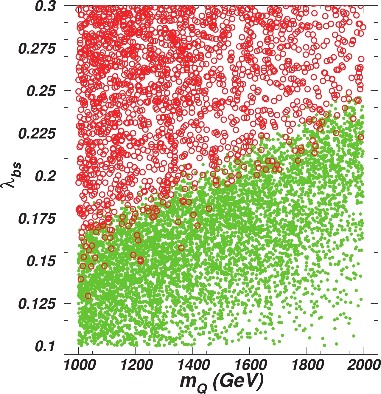
Figure 1. (color online) Remaining samples projected on the plane of
$ m_Q $ versus$ \lambda_{bs} $ . All the samples accomodate the$ R_{K^{(*)}} $ anomaly, and the bullets (green) and circles (red) are, respectively, the samples allowed and excluded by$ \Delta m_s $ .After imposing the relevant
$ b\to s $ flavor observables, neutrino trident process, and theoretical constraints, the samples explaining the$ R_{K^{(*)}} $ anomaly are projected on Fig. 2. The left panel shows that the parameters$ g_{Z'}q_X $ and$ m_{Z'} $ are imposed with strong constraints. Due to the constraints of the neutrino trident process, the region with small$ m_{Z'} $ and large$ g_{Z'}q_X $ is empty. To accomodate the$ R_{K^{(*)}} $ anomaly,$ m_{Z'} $ must increase with$ g_{Z'}q_X $ . Since we take$ g_{Z'}q_x \leqslant 1 $ to maintain the perturbativity of the$ Z' $ couplings,$ m_{Z'} > $ 600 GeV is excluded. Similarly,$ g_{Z'}q_x \leqslant 0.2 $ is disfavored since the minimal value of$ m_{Z'} $ is taken as 100 GeV.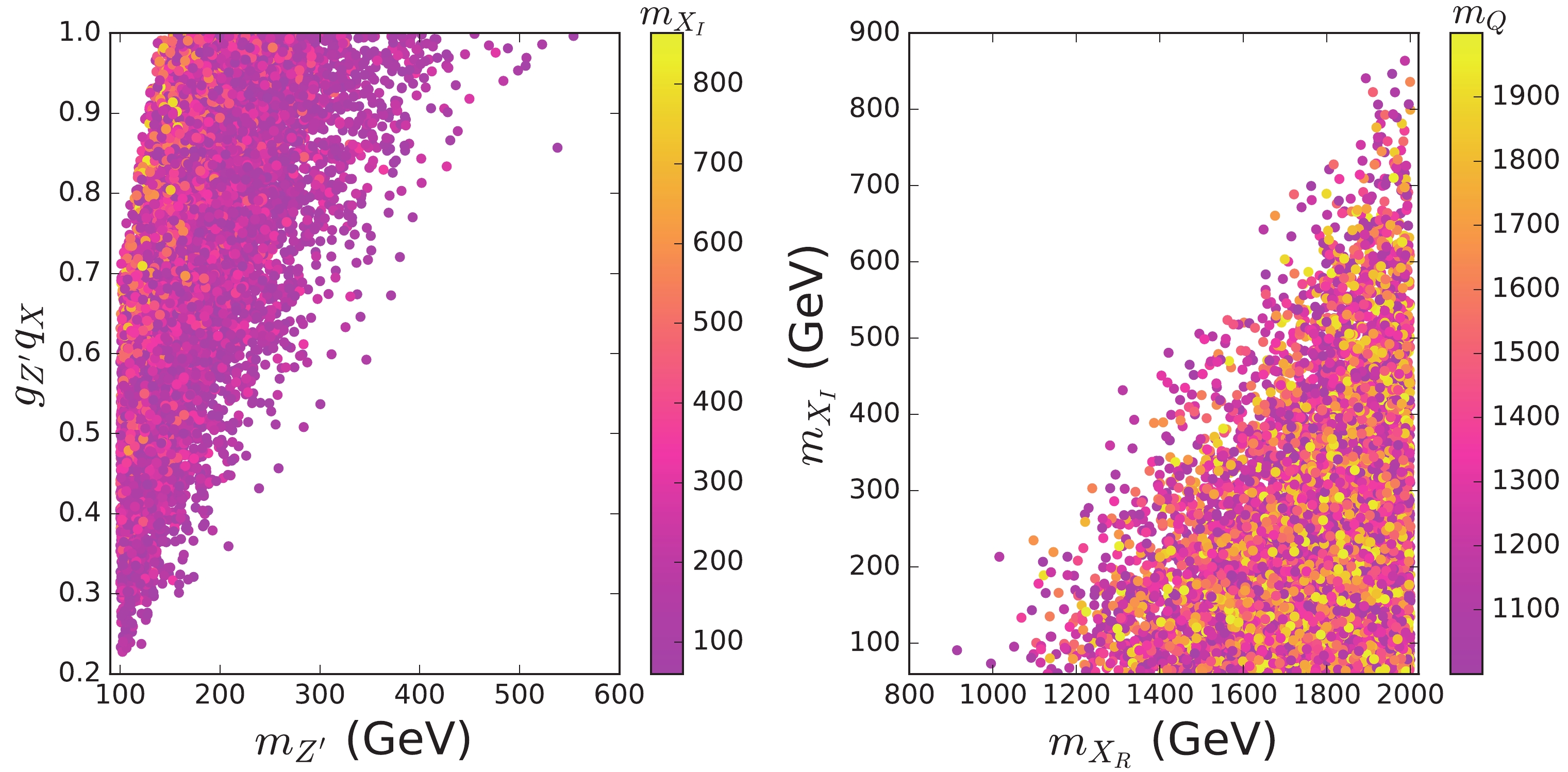
Figure 2. (color online) All the samples accomodate the
$ R_{K^{(*)}} $ anomaly and satisfy the relevant$ b\to s $ flavor observables, neutrino trident process, and theoretical constraints.The right panel of Fig. 2 shows that
$ m_{X_I} $ must increase with$ m_{X_R} $ since a sizable mass splitting between$ m_{X_R} $ and$ m_{X_I} $ is favoured to explain the$ R_{K^{(*)}} $ anomaly. Because we choose$ m_{X_R}\leqslant $ 2 TeV,$ m_{X_I} $ must be smaller than 900 GeV. Similarly,$ m_{X_R}\leqslant $ 800 GeV is disfavored since the minimal value of$ m_{X_I} $ is taken as 60 GeV. -
In the chosen parameter space, the DM can be annihilated into
$ Z'Z' $ ,$ SS $ , and the SM quarks. The corresponding Feynman diagrams are shown in Fig. 3. The$ X_IX_I\to q\bar{q} $ processes proceed through the$ D(U) $ -exchanging t-channel diagrams. For 1 TeV$ \leqslant m_Q\leqslant $ 2 TeV,$ \lambda_b<1 $ , and$ \lambda_s<1 $ , the annihilation cross sections are very small, and their contributions to the relic density can be ignored. The$ X_IX_I\to SS $ processes proceed through the S-exchanging s-channel diagram and the diagram of the quartic coupling$ X_IX_ISS $ . The$ X_IX_I\to Z'Z' $ processes proceed through the S-exchanging s-channel diagram,$ X_R $ -exchanging t-channel diagram, and diagram of the quartic coupling$ X_IX_I Z'Z' $ .
Figure 3. Feynman diagrams of
$ X_IX_I\to Z'Z',\; SS,\; q\bar{q} $ processes.We use
$ \textsf{micrOMEGAs} $ [27] to calculate the relic density and the spin-independent DM-nucleon cross section. The model file is generated by$ \textsf{FeynRules} $ [28]. The Planck collaboration reported the relic density of cold DM in the universe as$ \Omega_{c}h^2 = 0.1198 \pm 0.0015 $ [29].The annihilation cross section of
$ X_IX_I\to Z'Z' $ from the diagram shown in Fig. 3(c) only depends on the parameters$ g_{Z'}q_X $ ,$ m_{Z'} $ , and$ m_{X_I} $ . Since the$ R_{K^{(*)}} $ anomaly imposes a lower bound on$ g_{Z'}q_X $ , our calculations show that the annihilation cross sections of$ X_IX_I\to Z'Z' $ are much larger than the value that produces the correct relic density for$ m_{Z'}<m_{X_I} $ . Similarly, we find that the annihilation cross sections of$ X_IX_I\to SS $ are too large to obtain the correct relic density for$ m_{S}<m_{X_I} $ . The main reason is that the$ R_{K^{(*)}} $ anomaly imposes a low bound on the$ SX_IX_I $ coupling. The$ R_{K^{(*)}} $ anomaly requires a large mass splitting between$ X_R $ and$ X_I $ and imposes a lower bound on the parameter$ \mu $ according to Eq. (8):$ \sqrt{2}\mu = \frac{m^2_{X_R}-m^2_{X_I}}{2v_S}. $

(31) From Eq. (10), we can obtain the coupling of
$ SX_IX_I $ for the chosen parameters:$ \lambda_{SX_IX_I} = \sqrt{2}\mu-\lambda_{SX}v_S. $

(32) The remaing samples that explain the
$ R_{K^{(*)}} $ anomaly in Fig. 2 are projected on the planes of$ \lambda_{SX_IX_I} $ versus$ \lambda_{SX} $ and$ m_{S}-m_{X_I} $ in Fig. 4. From Fig. 4, we find that the$ R_{K^{(*)}} $ anomaly requires$ \sqrt{2}\mu> $ 3500 GeV, which dominates the value of$ \lambda_{SX_IX_I} $ .$ \lambda_{SX_IX_I} $ tends to decrease with increasing$ \lambda_{SX} $ and$ v_S $ , and$ \lambda_{SX_IX_I} $ is reduced to around 1000 GeV for$ \lambda_{SX}\approx 4\pi $ and$ v_S\approx 400 $ GeV. Meanwhile, a large$ v_S $ can increase$ m_S $ , leading to$ m_S > m_{X_I} $ . The right-most panel in Fig. 4 shows that the minimal value of$ \lambda_{SX_IX_I} $ is approximately 4000 GeV for$ m_S < m_{X_I} $ .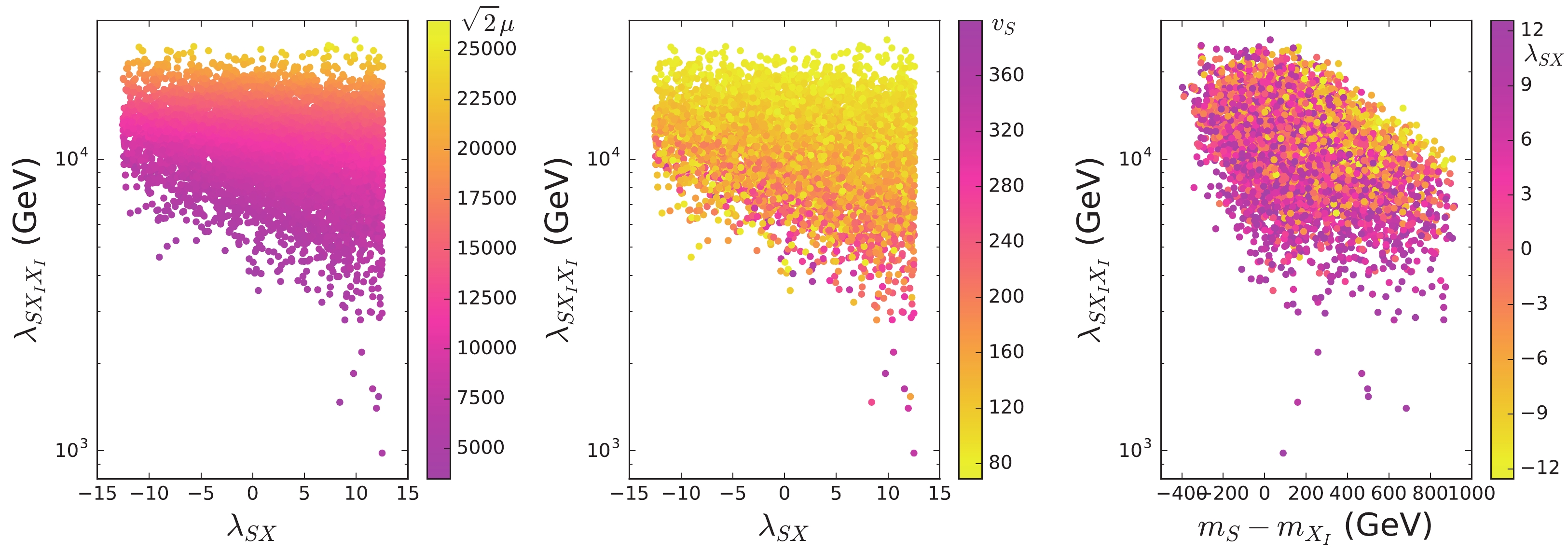
Figure 4. (color online) Same as Fig. 2 but projected on the planes of
$ \lambda_{SX_IX_I} $ versus$ \lambda_{SX} $ and$ m_{S}-m_{X_I} $ .To produce the relic density via the
$ X_IX_I\to Z'Z', SS $ annihilation processes, we need to use the effects of forbidden channel, namely that$ m_{Z'} $ or$ m_{S} $ is appropriately larger than$ m_{X_I} $ . In the calculation of the thermal averaged cross section, the early universe kinetic energy of the DM is nonnegligible. When the mass difference is not too large and the DMs move fast, the center of mass energy exceeds twice$ m_{Z'} $ or$ m_{S} $ . Therefore, the process$ X_IX_I\to Z'Z'\; (SS) $ can occur in the early universe when$ m_{X_I} $ is appropriately different from$ m_{Z'} $ ($ m_S $ ). In addition, the temperature at the present time is much lower than the freeze-out temperature, and the velocity of DM is much smaller than that in the early universe. The channels$ X_IX_I\to Z'Z'\; (SS) $ are kinematically forbidden at the present time; therefore, the experimental constraints of the indirect detection of DM can be naturally satisfied.After imposing the constraints of "pre-DM" (denoting the
$ R_{K^{(*)}} $ anomaly, relevant$ b\to s $ flavor observables, neutrino trident process, and theoretical constraints), we find some samples that can produce the correct DM relic density. The remaining samples are projected in Fig. 5. From the left panel, we find that the relic density favors$ m_{X_I}< $ 350 GeV and most of the surviving samples lie in the region where$ m_{Z'}-m_{X_I}<60 $ GeV. For a large$ m_S $ , the annihilation cross section of$ X_IX_I\to Z'Z' $ from the diagram in Fig. 3(a) is suppressed. Therefore, a small value of$ m_{Z'}-m_{X_I} $ is required to enhance the cross section. For a large value of$ m_{Z'}-m_{X_I} $ , the$ X_IX_I\to Z'Z' $ channel is still forbidden in the early universe and does not contribute to the relic density. For such a case, the$ X_IX_I\to SS $ channel will have the dominant contribution to the relic density. As shown in the right panel, for a large value of$ m_{Z'}-m_{X_I} $ , a small value of$ m_{S}-m_{X_I} $ is required to allow the$ X_IX_I\to SS $ channel in the early universe.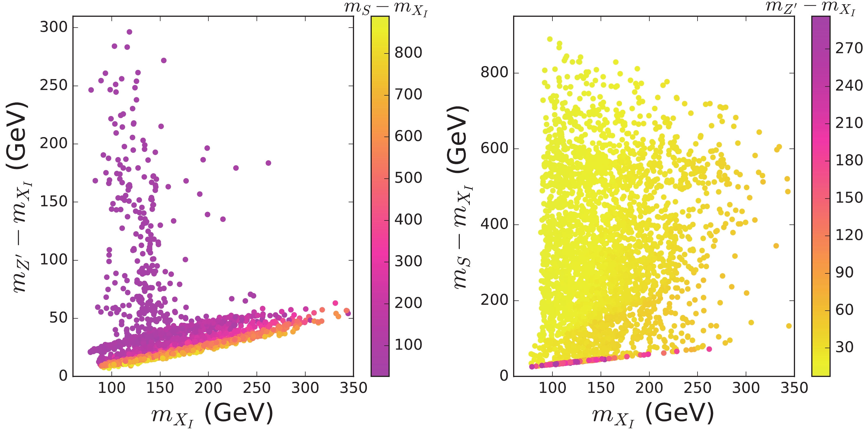
Figure 5. (color online) Remaining samples satisfying the DM relic density and the constraints of "pre-DM."
Exchanging an initial state
$ X_I $ and a final state quark shown in Fig. 3(f), we can obtain the Feynman diagrams that contribute to the cross section of the DM scattering off the nuclei. In the chosen parameter space, we find that the bounds of the XENON1T fail to exclude the parameter space that achieves the correct relic density [30]. -
At the LHC, the vector-like quarks D and U are produced in pairs via the QCD processes
$ pp\to D\bar{D}, U\bar{U}. $

(33) In the chosen parameter space, D and U have the following decay modes:
$ D\to X_I d_i, X_R d_i,\; \; \; U\to X_I u_i, X_R u_i $

(34) with
$ X_R\to X_I Z'\to X_I \mu^+ \mu^-,~ X_I\tau^+\tau^-,~ X_I\nu_\mu \bar{\nu}_\mu,~ X_I\nu_\tau \bar{\nu}_\tau. $

(35) Since the
$ R_{K^{(*)}} $ anomaly and the DM relic density favor$ X_R $ to be much larger than$ X_I $ , D and U will mainly decay into$ X_Is $ ,$ X_Ib $ , and$ X_Iu_i $ . In this paper, the coupling of$ X_I $ and the d quark is taken as zero.In order to restrict the products of the above processes at the LHC for our model, we perform simulations for the samples using
$ \texttt{MG5}\_\texttt{aMC-2.7.3} $ [31] with$ \texttt{PYTHIA8} $ [32] and$ \texttt{Delphes-3.2.0} $ [33], and adopt the constraints from all the 13 TeV LHC analysis in the version$ \texttt{CheckMATE 2.0.28} $ [34]. For the excluded samples, the most sensitive experimental analysis is the ATLAS search for squarks and gluinos in final states that contain jets and missing transverse momentum at the 13 TeV LHC with 139 fb$ ^{-1} $ integrated luminosity data [35]. The final states$E_T^{\rm miss}$ +${\rm jets}$ are just the main signals of$ D\bar{D} $ and$ U\bar{U} $ in the model.In Fig. 6, all the samples satisfy the constraints of the "pre-DM" and DM observables. Current direct searches at the LHC exclude
$ m_Q< $ 1.7 TeV. For a large$ \lambda_s $ , some samples with$ m_Q $ around 1.8 TeV can also be excluded. With an increase of$ m_Q $ , the production cross sections of$ pp\to D\bar{D},\; U\bar{U} $ are suppressed by the phase space, and the direct searches at the LHC can be satisfied.
Figure 6. (color online) All the samples satisfy the constraints of the "pre-DM" and DM observables. The squares and bullets indicate, respectively, the samples excluded and allowed by the current direct searches at the LHC.
-
Since the vector-like quarks U and D are charged under
$ U(1)_{L_\mu-L_\tau} $ , the gauge boson$ Z' $ has tree-level couplings to the vector-like quarks. Therefore, the model provides a novel approach of searching for$ Z' $ , the vector-like quark, and DM.$ Z' $ is produced via the QCD process followed by$ D\to s (b) X_I $ ,$ D\to s (b) X_R \to $ $ s (b) Z'X_I $ , and then$ Z'\to\mu^+\mu^- $ .We pick a benchmark point which accomodates the
$ b\to s\mu^+\mu^- $ anomaly and satisfies the constraints of "pre-DM," the DM observables, and the current searches at the LHC. Several key input and output parameters are shown in Table 3. Now we perform detailed simulations on the signal and backgrounds at the 14 TeV LHC with high luminosity. We choose the signal to contain an opposite sign di-muon ($ \mu^+\mu^- $ ), missing transverse momentum$E^{\rm miss}_T$ , and multijets ($ \geqslant $ 2 jets), which include at least one b-jet. The major SM irreducible background processes to this signal are$ t\bar{t} $ ,$ WW+ $ jets,$ ZZ+ $ jets, and$ WZ+ $ jets.$ m_{Z'} $ /GeV

$ m_{X_I} $ /GeV

$ m_{X_R} $ /GeV

$ m_Q $ /GeV

${\rm Br}(D\to X_Ib)$ 

${\rm Br}(D\to X_Is)$ 

${\rm Br}(D\to X_Rb)$ 

${\rm Br}(D\to X_Rs)$ 

170 145 1309 1930 0.63 0.14 0.19 0.04 Table 3. Several key input and output parameters for the benchmark point.
We identify muon candidates by requiring them to have
$ p_T>15 $ GeV and$ |\eta|<2.5 $ . The anti-kt algorithm is employed to reconstruct jets with a radius parameter$ R = 0.4 $ [36], and the jets are required to have$ p_T>20 $ GeV and$ |\eta|<2.5 $ . We assume an average b-tagging efficiency of 80% for real b-jets.In order to suppress the contributions from the SM process, we apply the "stransverse" mass
$ m_{T2} $ [37-39] defined as$ {m_{T2}} = {\min _\limits{{{{q}}_{{T}}}}}\left[ {\max \left( {{m_T}({{p}}_{{T}}^{{\ell _{\bf{1}}}},{{{q}}_{{T}}}),{m_T}({{p}}_{\bf{T}}^{{\ell _{\bf{2}}}},{{p}}_{{T}}^{{\rm miss}} - {{{q}}_{{T}}})} \right)} \right], $

(36) where
${{p}}_{{T}}^{{\ell _{\bf{1}}}}$ and${{p}}_{{T}}^{{\ell _{\bf{2}}}}$ are the transverse momenta of the di-muon.${{{q}}_{{T}}}$ is a transverse vector that minimizes the larger of the two transverse masses$ m_T $ :$ {m_T}({{{p}}_{{T}}},{{{q}}_{{T}}}) = \sqrt {2({p_T}{q_T} - {{{p}}_{{T}}} \cdot {{{q}}_{{T}}})} . $

(37) Figure 7 shows the distributions of some kinematical variables at the LHC with
$ \sqrt{s} = 14 $ TeV for the signal and the background$ t\bar{t} $ . The other processes are not shown since they are subdominant. According to the distribution differences between the signal and backgrounds, we can improve the ratio of signal to background by making some kinematical cuts. We impose the following cuts: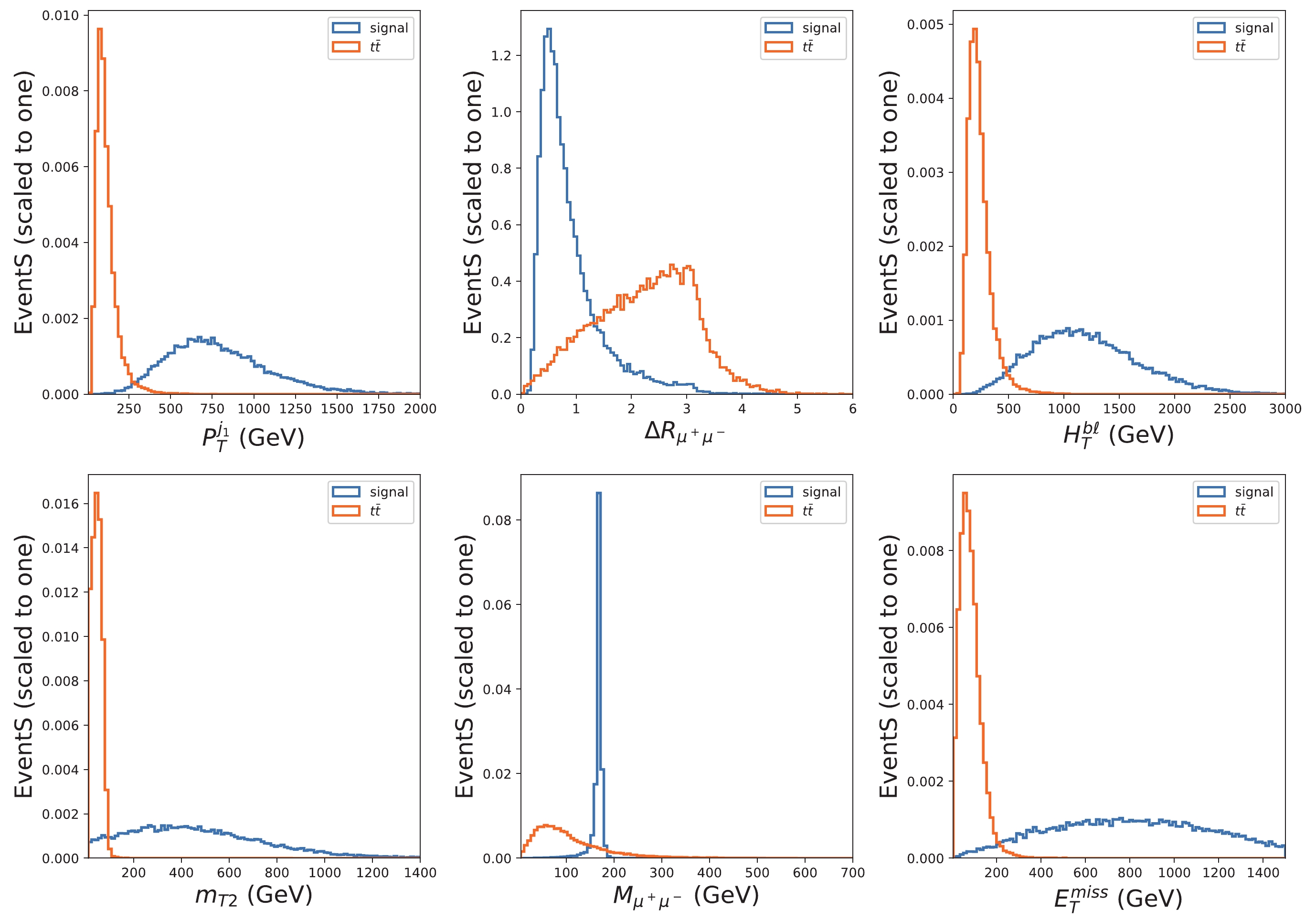
Figure 7. (color online) Signal and
$ t\bar{t} $ background distributions of$ P_T^{j_1,} $ ,$ \Delta R_{\mu^+\mu^-} $ ,$ H_T^{b\ell} $ ,$ m_{T2} $ ,$ M_{\mu^+\mu^-} $ , and$E_T^{\rm miss}$ at the 14 TeV LHC after requiring an opposite sign di-muon and multijets ($ \geq $ 2 jets), which include at least one b-jet.$ \begin{aligned}[b] &P_T^{j_1} > 290\; {\rm GeV},\; \; P_T^{j_2} > 60\; {\rm GeV},\; \; P_T^{b_1} > 60\; {\rm GeV},\\ &\Delta R_{\mu^+\mu^-} < 2.0,\; \; 150\; {\rm GeV} < M_{\mu^+\mu^-} < 180\; {\rm GeV},\\ &E_T^{\rm miss} > 310 \;{\rm GeV},\; \; m_{T2} > 100\; {\rm GeV},\; \; H_T^{b\ell} > 500\; {\rm GeV}. \end{aligned} $

(38) Here,
$ P_T^{j_1} $ and$ P_T^{j_2} $ denote the transverse momentum of the hardest and the second hardest jets, which include the b-jet, and$ P_T^{b_1} $ denotes the transverse momentum of the hardest b-jet.$ \Delta R = \sqrt{(\Delta \phi)^2+(\Delta \eta)^2} $ is the particle separation with$ \Delta \phi $ and$ \Delta \eta $ being the separation in the azimuthal angle and rapidity, respectively.$ M_{\mu^+\mu^-} $ is the invariant mass of$ \mu^+ $ and$ \mu^- $ , and$ H_T^{b\ell} $ is a scalar sum of the transverse momenta of all the b-jets,$ \mu^\pm $ . Since$ \mu^+ $ and$ \mu^- $ of the signal are from the decay of$ Z^\prime $ with a mass of$ 170 $ GeV, a$ M_{\mu^+\mu^-} $ peak appears at 170 GeV, and$ \Delta R_{\mu^+\mu^-} $ favors a small value. The jets,$ X_I $ , and$ \mu^\pm $ of the signal are the decay products of the vector-like quark with a mass of 1930 GeV, and such a heavy mass results in these products tending to have large transverse momenta. The distributions of$ m_{T2} $ for$ t\bar{t} $ and$ WW $ +jets backgrounds peak before$ m_W $ . In addition, the DM$ X_I $ has a mass of 145 GeV, therefore the signal events tend to have a large$E_T^{\rm miss}$ .We compute the significance as
$ \mathbf{S} = \dfrac{n_s}{\sqrt{n_s+n_b}} $ , where$ n_s $ and$ n_b $ are the normalized signal and background event yields, respectively. After making the kinematical cuts of Eq. (38),$ n_b $ is drastically reduced and dominated by$ n_s $ . For example,$ n_s\sim 33 $ and$ n_s + n_b \sim 35 $ for a dataset wtih 3000 fb$ ^{-1} $ at the 14 TeV LHC. Figure 8 shows that, for the benchmark point, the significance can reach 2$ \sigma $ and 5.6$ \sigma $ at the 14 TeV LHC with integrated luminosities 400 fb$ ^{-1} $ and 3000 fb$ ^{-1} $ .
Figure 8. (color online) Significance versus integrated luminosity of the 14 TeV LHC for the benchmark point.
The gauge boson
$ Z' $ is also produced via$ pp\to D\bar{D} $ followed by both D decays to$ X_R $ , i.e.$ D\to s(b) X_R\to $ $ s(b) Z'X_I $ and$ \bar{D}\to \bar{s}(\bar{b}) X_R\to \bar{s}(\bar{b}) Z'X_I $ . Because of two$ Z' $ in this channel, the final signal contains two di-muons, missing transverse momentum$E^{\rm miss}_T$ , and multijets ($ \geqslant $ 2 jets). Since the$ R_{K^{(*)}} $ anomaly requires$ m_{X_R} $ to be much larger than$ m_{X_I} $ ,${\rm Br} [D\to s(b) X_R]$ is much smaller than${\rm Br}[D\to s(b) X_I]$ . In addition, the second$ Z' $ decay into$ \mu^+\mu^- $ will lead to an additional suppression factor of$ \dfrac{1}{3} $ . Taking the benchmark point in Table 3 as an example, we can obtain$ \frac{{\rm Br}(D\bar{D}\to b\bar{b} X_I X_R \to b\bar{b} X_I X_I Z' \to b\bar{b} X_I X_I \mu^+\mu^-)} {{\rm Br}(D\bar{D}\!\to\! b\bar{b} X_R X_R \!\to\! b\bar{b} X_I X_I Z' Z'\!\to\! b\bar{b} X_I X_I \mu^+\mu^-\mu^+\mu^-)}\!\approx\! 20. $

(39) Although the two di-muons of the
$ D\bar{D}\to X_R X_R b\bar{b} $ channel can be used to suppress the background events more efficiently, the number of signal events is approximately one twentieth of that of the$ D\bar{D}\to X_I X_R b\bar{b} $ channel. Therefore, the channel studied in detail in this paper is more promising for probing$ Z' $ than the channel of both D decays to$ X_R $ . -
In this study, we investigate the capability of the LHC to test DM,
$ Z^{\prime} $ , and vector-like quarks in a local$ U(1)_{L_\mu-L_\tau} $ model in light of the$ b\to s\mu^+\mu^- $ anomaly and DM observables. We take$ m_Q< $ 2 TeV and$ m_{X_R}< $ 2 TeV and find that the$ b\to s\mu^+\mu^- $ anomaly and the DM observables favor$ m_{X_I}< 350 $ GeV and$ m_{Z^{\prime}}< 450 $ GeV after imposing relevant constraints from theory and$ b\to s $ flavor observables. The current searches for jets and missing transverse momentum at the 13 TeV LHC with 139 fb$ ^{-1} $ integrated luminosity data exclude$ m_Q< $ 1.7 TeV. Finally, we propose a novel channel for probing these new particles at the high luminosity LHC via the QCD process$ pp \to D\bar{D} $ followed by$ D\to s (b) X_I $ ,$ D\to s (b) Z'X_I $ , and then$ Z'\to\mu^+\mu^- $ . Taking a benchmark point of$ m_Q $ = 1.93 TeV,$ m_{Z^\prime} = 170 $ GeV, and$ m_{X_I} = $ 145 GeV, we perform a detailed Monte Carlo simulation and find that this benchmark point can be accessed at the 14 TeV LHC with an integrated luminosity 3000 fb$ ^{-1} $ . -
We thank Biaofeng Hou for the helpful discussions.
Dark matter, Z′, and vector-like quark at the LHC and b → sμμ anomaly
- Received Date: 2021-02-21
- Available Online: 2021-08-15
Abstract: Combining the


 DownLoad: