


 Abstract
 HTML
HTML Reference
 Related
 PDF
PDF


-
The spectacular discovery of the chargeless Higgs particle
$ (H^0) $ at the LHC [1-3] is consistent with the prediction of the Standard Model (SM), confirming the basic concept of the spontaneous symmetry breaking mechanism and elementary particle mass generation. The observed$ H^0 $ decay into gauge boson particles$ W^+W^- $ and$ ZZ $ [4-6] fits beautifully into this picture. Similarly, determination of$ t \bar t H^0 $ couplings in gluon fusion [7-9] and$ t\bar t H^0 $ production [10] confirm the role of the Higgs boson in fermion mass generation. With gathered statistics, we know more and more about this particle, namely, its decay rate to$ \gamma \gamma $ [11, 12] and its spin-parity, which is predominantly$ J^P = 0^+ $ [4, 5, 13-15]. Moreover, the mass suppressed decay rate to muon pairs when compared with top pairs is evident [12, 16]. Yet another spectacular success of the LHC physics is the clear discovery that the Higgs boson decays to the third generation of fermions, namely to the pairs of τ leptons and b-quarks. In particular, determination of the Yukawa Higgs boson coupling to b-quarks is tricky, as even though this channel amounts to approximately 60% of Higgs boson decays, the QCD b-quark background is overwhelming [17]. The story of Higgs boson studies continues. Very recently, measurements of the Higgs boson’s properties have reached a new stage in precision through detection of a rare decay mode where the Higgs boson decays into two muons [18, 19]. Aiming at sub-percent precision for Higgs boson decays, quantitative tests of the SM for Higgs boson couplings require further scrutinization in studies at HL-LHC and future Higgs factories. This includes investigation of the Higgs boson self-coupling [20]. -
Detection of the Standard Model scalar particle does not preclude the validity of more elaborate physical scenarios with extended scalar sectors. The simplest extensions beyond the SM doublet scalar multiplet include their copies, like the two Higgs doublet model [21], supersymmetric extensions of the SM [22, 23] or, stepping up in this construction, scenarios with triplet scalar representations, either in their supersymmetric [24, 25] or non-supersymmetric versions [26-28]. Here, we will consider the latter. There are many possibilities for triplet representations, depending on the hypercharge
$ Y\equiv $ $ 2(Q-T_3) $ [29-32]. We will explore the simplest one, which involves doubly charged Higgs fields in triplet representation with hypercharge$ Y = 2 $ , i.e., the Higgs Triplet Model ($ {\texttt{HTM}}$ ) [33]. To accomplish this, we will not assume any special symmetries or constructions [34, 35], so that$ v_{\Delta} $ , the triplet vacuum expectation value (VEV), will be extremely tiny, at the scale of electronvolts, which makes experiments more challenging. We will also consider a much more complex model, where the Standard Model$ SU(2)\times U(1) $ gauge symmetry is extended by an additional$ SU(2) $ group, the so-called minimal left-right symmetric model ($ {\texttt{MLRSM}}$ ) [28, 36-40]. Thus, we consider a setting where both the$ {\texttt{HTM}}$ and$ {\texttt{MLRSM}}$ include doubly charged Higgs bosons.$ {\texttt{HTM}}$ has received a considerable amount of attention recently [41-54]. When confronted with experimental data, this model features a strong restriction in which$ v_{\Delta} $ is very small,$ {{\cal{O}} \left(1 \right)} $ (GeV) or below. Here, in particular, we concentrate on the cases where$ v_{\Delta} $ is on the order of neutrino masses. Then, the triplet Yukawa couplings will be on the$ {{\cal{O}} \left(1 \right)} $ order and$ H^{\pm\pm} $ decays dominantly into the same-sign dilepton channel. In this case, the LHC direct search bound on the doubly charged scalar mass,$ m_{H^{\pm \pm}}\gtrsim 850 $ GeV [55] applies. At the same time, the constraints from different lepton flavor violating (LFV) processes and non-universality of leptonic couplings begin to weigh in. There is thus a direct relationship among the triplet VEV$ v_{\Delta} $ , neutrino masses, their mixing, and doubly charged Higgs couplings. That is why the production and decays of$ H^{\pm \pm} $ scalars at high energies depend substantially on the oscillation data and limits on LFV processes in the$ {\texttt{HTM}}$ .In the
$ {\texttt{MLRSM}}$ , the dominating non-standard effects in phenomenological studies are connected with the right-handed breaking scale$ v_R $ , which affects the couplings and masses of a wide set of non-standard heavy particles of spins 0, 1, and 1/2 present in the model. Low-energy precision SM and rare processes, as well as high-energy collider studies, limit the possible values of$ v_R $ from below. The scale of relevance for$ v_R $ begins at the$ {{\cal{O}} \left(1 \right)} $ TeV level [56].Consequently, in both models, we have two completely different VEV scales,
$ v_{\Delta} $ and$ v_R $ . How can we discriminate such two distinct models experimentally? Indeed, it is not easy, as any non-standard effect considered or thought of so far in phenomenological studies in the search for BSM models has failed to show unambiguous excess rates (reported excesses were vanishing with higher statistics).One of the most appealing rare processes capable of exposing BSM signals involving doubly charged Higgs bosons at high energy colliders would be the
$ H^{\pm \pm} $ pair production and the subsequent decays to four charged leptons. Here, the same charge sign dileptons appear from the parent's$ H^{\pm \pm} $ ,$ H^{\pm \pm} \to l^\pm l^\pm $ , which is distinguishable from the SM background. In addition, we compare the$ H^{\pm \pm} $ production and decay signals in the two considered BSM models, taking into account all relevant experimental limits. In this work, we investigate this scenario in detail.The
$ {\texttt{HTM}}$ model that we discuss is the simplest theoretical scenario with the triplet scalar representation, without ad-hoc symmetries added. On the opposite side of the theoretical complexity stands the$ {\texttt{MLRSM}}$ model. This model poses a broad spectrum of non-standard features: an additional gauge group, including other gauge bosons and right-handed currents, heavy neutral leptons, and a plethora of Higgs scalars, including two doubly charged Higgs bosons$ H_{(1,2)}^{\pm \pm} $ . Details on scalar potentials and fields are given in the Appendix. Additionally, as already mentioned, the process of$ H_{}^{\pm \pm} $ pair production at colliders is peculiar because it exhibits a small background. We assume a scenario in which the excess signal of four charged leptons$e^+ e^- (pp) \to H_{}^{++} H_{}^{--} \to 4l$ over the background is identified. In the case where no other non-standard signals appear (e.g., connected with right-handed currents), the question is how to find the non-standard model to which the signal belongs. In practice, such identification will be not trivial. In our opinion, the problem of distinguishing two models based on rare processes where particles with the same masses play a crucial role is an important topic; needless to say, such statements are essential for future post-LHC studies. Usually in phenomenological analysis, any specific models are considered. The exception is the effective field theory approach, where non-standard interactions and energy scales are probed. However, regarding specific models, if positive signals and deviations from the SM signals are found, comparative studies as given here based on particular models will be crucial. Apart from these general statements, other exciting subtleties can be probed in these studies connected with the neutrino sector. We will come to this topic in a moment.To obtain reliable predictions for BSM processes, essential restrictions on the BSM model parameters coming from rare and so far not observed LFV processes must be considered. As even a single unambiguous LFV event detection would be a signal beyond SM physics, there are many efforts to upgrade or create new experimental setups for that; see, e.g., [57, 58]. Present bounds for low energy LFV signals, such as nuclear μ to e conversion, will become more stringent through the so-called intensity frontier experiments [59, 60]. The same is true for
$ (\beta \beta)_{0 \nu} $ experiments; see, e.g., [61, 62]. In this work, we consider these processes to predict reliable BSM$ H^{\pm \pm} $ collider signals.Concerning high energy colliders, there are presently several options considered internationally for future electron colliders [63], namely the Future Circular Collider (FCC) [64, 65], Compact Linear Collider (CLIC) [66, 67] – both at CERN– and the International Linear Collider (ILC ①) [69, 70]. The Chinese Electron Positron Collider (CEPC) [71, 72] in China is of the circular type and, similar to the FCC, is expected to collide electrons with positrons at center of mass energies of 90-365 GeV. The ILC collider could potentially be positioned in Japan, and its center of mass collision energies would reach 1 TeV, while the CLIC would cover the energies between 380 GeV and 3 TeV. In the future, extreme energies may become possible in Plasma Wakefield Linear Colliders [73]. In the case of the FCC-ee, four running stages are considered [64, 74, 75], with a focus on Z, W, H, and top quark production. This means that the maximal energy will be not sufficient to search for direct
$ H^{\pm \pm} $ pair production signals. What remains is the high luminosity LHC (HL-LHC) [63, 76] and the FCC-hh proton-proton option with center of mass energies of collided protons reaching 100 TeV [77, 78].A significant portion of the calculations in this paper was performed using the MadGraph [79] and Pythia [80, 81] programs. The UFO files were generated using FeynRules [82] and built on our model file, based on the default SM implementation.
-
Regarding the scalar particle masses, we have constructed a mass spectrum in which
$ M_{H^{\pm\pm}} = 700 $ GeV. Corresponding parameters of scalar potentials in both models are given in Table 1.$ {\texttt{HTM}}$ 

$\mu = 1.7 \times 10^{-7}, \quad \lambda = 0.519, \quad \lambda_1 = 0.519, \quad \lambda_2 = 0, \quad \lambda_3 = -1, \quad \lambda_4 = 0.$ 

$M_{h}$ = 125.3 GeV,

$M_{H}$ = 700 GeV,

$M_{H^\pm}$ = 700 GeV,

$M_{H^{\pm\pm}}$ = 700 GeV.

$ {\texttt{MLRSM}}$ 

$\lambda_1 = 0.129, \; \rho_1 = 0.0037, \; \rho_2 = 0.0037, \; \rho_3-2\rho_1 = 0.015, \; \alpha_3 = 4.0816, \; 2\lambda_2 - \lambda_3 = 0$ .

$M_{H_0^0}$ = 125.3 GeV,

$M_{H_1^0}$ = 10 TeV,

$M_{H_2^0}$ = 600 GeV,

$M_{H_3^0}$ = 605.4 GeV,

$M_{H_1^{\pm\pm}}$ = 700 GeV,

$M_{H_2^{\pm\pm}}$ = 700 GeV,

$M_{H_1^\pm}$ = 654.4 GeV,

$M_{H_2^\pm}$ = 10 003.1 GeV.

Table 1. Benchmark points and corresponding potential parameters for
$ {\texttt{HTM}}$ and$ {\texttt{LRSM}}$ with$M_{H^{\pm\pm}}=M_{H^{\pm\pm}_{1,2}}$ = 700 GeV. The scalar potential parameters, fields, and relations for masses are defined in the Appendix, Eq. (A1) and Eq. (A19). We identify h and$H_0^0$ as the SM Higgs boson ($H^0$ ).The mass benchmark points are constructed to satisfy several theoretical conditions, including potential stability, unitarity, and the T-parameter restriction and bounds from
$ h \to \gamma \gamma $ [45, 56, 83-86]; see also Sections III and IV.As we can see in Table 1, there are more scalar fields in the
$ {\texttt{MLRSM}}$ than in the$ {\texttt{HTM}}$ . Any detectable signal connected with a neutral, singly, or doubly charged Higgs bosons that are present in the$ {\texttt{MLRSM}}$ but are not present in the$ {\texttt{HTM}}$ would be in favor of the$ {\texttt{MLRSM}}$ . However, we should note that although the$ {\texttt{MLRSM}}$ is very rich in particle content and non-standard interactions, despite a great amount of theoretical and experimental efforts over the last several decades, what we have so far are exclusion limits on the parameters of this model. No experimental data considered so far indicate neutral, singly, or doubly charged scalars, extra neutral heavy leptons, or extra gauge bosons. Therefore, the starting point is actually the same: we do not know if and which BSM model is realized in nature, and we are still searching for a first experimental indication toward any non-standard signals in one or another model. As the models' parameters are already severely constrained, we have to consider very rare processes and hence faint signals. We focus on the cleanest BSM collider signal connected with doubly charged scalars: their pair production and subsequent decays (correlations between the same-sign leptons in the final state originating from$ H^{\pm \pm} $ decays). To leave no stone unturned, we will focus especially on the case in which two doubly charged Higgs bosons in the$ {\texttt{MLRSM}}$ have the same masses; otherwise, the second scalar$ H_2^{\pm \pm} $ connected with the right-handed triplet in the$ {\texttt{MLRSM}}$ (see the Appendix for field definitions) would help to discriminate between models in favor of the$ {\texttt{MLRSM}}$ . A case with different$ H_1^{\pm \pm} $ and$ H_2^{\pm \pm} $ masses in$ e^+e^- $ CLIC center of mass energies will be discussed in Section V.E, and non-degenerate mass cases for hadron colliders have been discussed already in [87]. For the same masses of$ H_1^{\pm \pm} $ and$ H_2^{\pm \pm} $ with the same masses, the production rates are higher in the$ {\texttt{MLRSM}}$ than they are in the$ {\texttt{HTM}}$ . We will determine the contribution of$ H_2^{\pm \pm} $ against$ H_1^{\pm \pm} $ in production processes at lepton and hadron colliders, in the case of the same doubly charged boson masses, and how these contributions change with center of mass energy. As we will see, there are scenarios with model parameters where the difference in signals for both models can be further enhanced by studying the leptonic branching ratios of doubly charged Higgs bosons and kinematic cuts.Fixing the scalar mass spectrum allows an initial inspection of the production processes
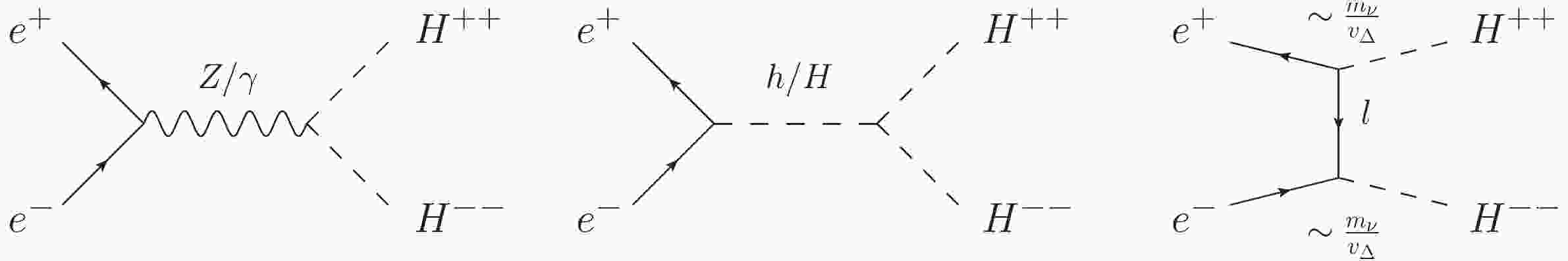
$e^+ e^- \to H_{(1,2)}^{++} H_{(1,2)}^{--}$ and$pp \to H_{(1,2)}^{++} H_{(1,2)}^{--}$ for the$ {\texttt{HTM}}$ and$ {\texttt{MLRSM}}$ . This will lead to discussion of the importance of the neutrino sector. Fig. 1 and Fig. 2 show classes of Feynman diagrams for the$ H^{\pm\pm} $ pair production in$ e^+e^- $ collisions in both models. These are s-channel diagrams mediated by neutral gauge bosons Z and γ and Higgs bosons, and the t-channel diagram. Because of experimental restrictions discussed in the next two sections, the contributions coming from the s-channel diagrams are comparable with the off-resonance regions, and the resonance regions for the considered center of mass energies and masses lie away from the allowed region of parameters (see Figs. 7 and 8). This provides the possibility to discuss how the t-channel diagrams in Fig. 1 and Fig. 2 affect the process.
Figure 1. Pair production of doubly charged Higgs bosons
$e^+ e^- \to H^{++} H^{--}$ in the$ {\texttt{HTM}}$ model. For the t-channel, the couplings depend on neutrino parameters and$v_\Delta$ . The exact form of the coupling is given by Eq. (3).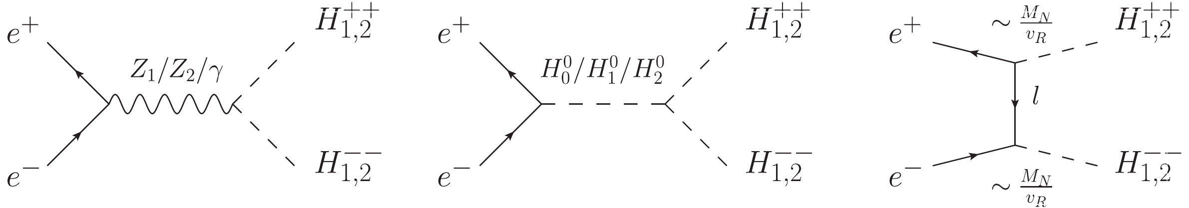
Figure 2. Feynman diagrams at the tree level for pair production of doubly charged Higgs bosons
$e^+ e^- \to H^{++} H^{--}$ in the${\texttt{MLRSM}}$ model. For the t-channel, the couplings depend on the heavy neutrino masses and$v_R$ . The exact form of the coupling is given by Eq. (4).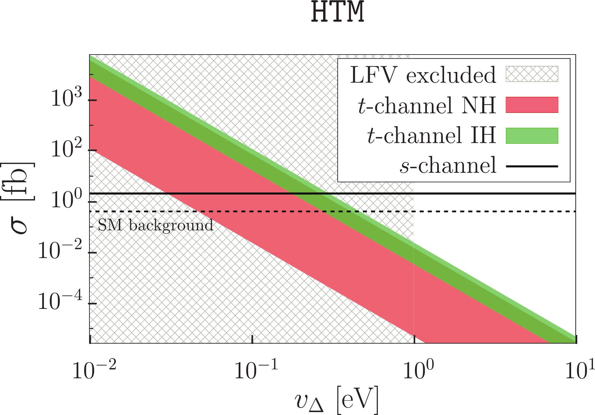
Figure 7. (color online) Doubly charged Higgs boson pair production
$e^+e^- \to H^{++} H^{--}$ for$M_{H^{\pm\pm}} =700$ GeV and CM energy 1.5 TeV in the$ {\texttt{HTM}}$ model. The crossed area is excluded by the low energy data (Table 5). We took the neutrino oscillation parameters within the$\pm 2 \sigma$ range (Table 4), which is why the t-channel is smeared. With a dashed line, we have marked the SM background for four lepton production (electrons and muons), which is$\sigma=0.415$ fb; see Section V.D.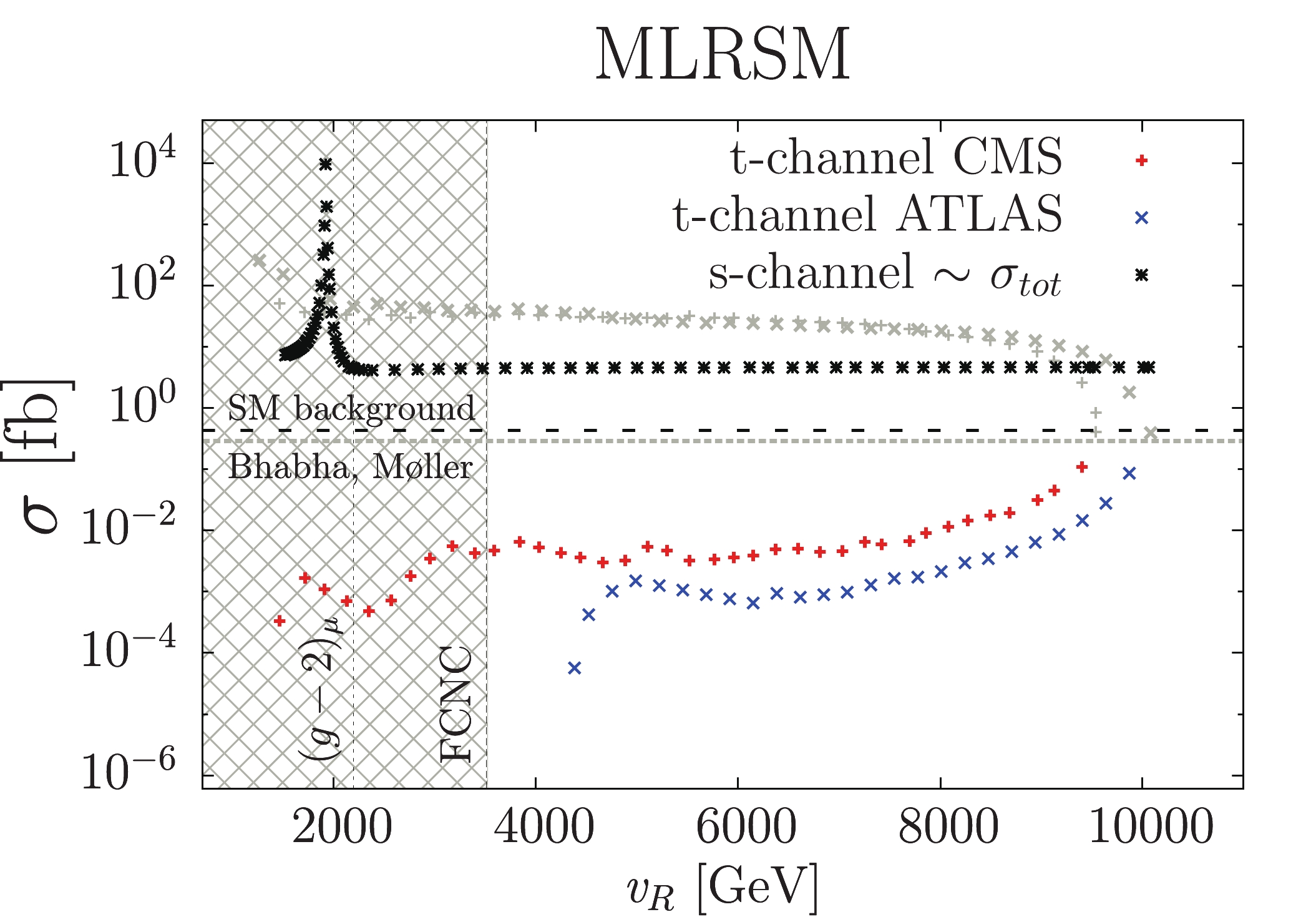
Figure 8. (color online) Doubly charged Higgs boson pair production
$e^+e^- \to H_1^{++} H_1^{--} + H_2^{++} H_2^{--}$ for$M_{H^{\pm\pm}_{(1,2)}} =700$ GeV and CM energy 1.5 TeV in the${\texttt{MLRSM}}$ . For the t-channel, the choice$M_{W_2}-M_N$ space is restricted by the LHC results best fit expected values; see Fig. 6. The crossed area on the left is excluded by$(g-2)_\mu$ and FCNC. The maximum for$v_R = 1900$ GeV comes from the$Z_2$ resonance,$M_{Z_2}=1.9$ TeV. The horizontal gray dashed line denoted "Bhabha, Møller" separates the t-channel contribution to the cross section, which is still allowed by the CMS and ATLAS exclusion analysis from constraints by the Bhabha and Møller processes (Table 2 and Table 3). The t-channel contribution above this line is forbidden. The SM background (black dashed horizontal line) after applying kinematic cuts is$\sigma =0.415$ fb; see Section V.D.As schematically depicted in the figures, the relevant
$ H^{\pm\pm}-l^{\mp}-l'^{\mp} $ vertices come from Yukawa couplings.In the
$ {\texttt{HTM}}$ , the Yukawa term (A6) with neutrino fields generates Majorana masses$ {\cal{L}}_Y^{\Delta} \rightarrow {\cal{L}}_\nu^{\Delta} = \frac{1}{2} \: \bar{\nu}_{\ell} \: \frac{v_{\Delta}}{\sqrt{2}} \: {\cal{Y}}_{\ell\ell'} \: \nu_{\ell'} \equiv \frac{1}{2} \: \bar{\nu}_{\ell} \: (M_\nu)_{_{\ell\ell'}} \: \nu_{\ell'} {.} $

(1) This term also contains the
$ H^{\pm\pm}-l^{\mp}-l'^{\mp} $ vertex, which leads to lepton flavor violation. We can diagonalize the neutrino mass matrix by U as follows [88]$ U^{\dagger} \: M_\nu \: U^* = \frac{1}{2} D_\nu = \frac{1}{2} \: {\rm{diag}}\{m_1, m_2, m_3\}. $

(2) The matrix U relates the mass eigenstates
$ | \nu_i \rangle $ through a superposition of the flavor states$ | \nu_\ell \rangle $ :$ |\nu_i \rangle = \; U^T |\nu_\ell \rangle $ , so it is directly connected to the$ {\texttt{PMNS}}$ matrix (11), and the exact relation between them is$U^* = V_{\rm PMNS}$ . Now, we can write the Yukawa couplings as a function of the$ {\texttt{PMNS}}$ matrix and the masses of neutrinos. From Eq. (2),$ {\cal{Y}}_{\ell\ell'} $ can be written in the following form$ {\cal{Y}}_{\ell\ell'} = \frac{1}{\sqrt{2} v_{\Delta}} \ V_{\texttt{PMNS}}^* \: D_\nu \: V_{\texttt{PMNS}}^{\dagger} . $

(3) We discuss the parametrization of
$ V_ {\texttt{PMNS}}$ and the emplo yed range of the oscillation parameters in Section III.A.The
$ {\cal{Y}}_{\ell\ell'} $ coupling depends on$ v_{\Delta} $ , neutrino masses, and oscillation parameters. From perturbativity,$ {\cal{Y}}_{\ell\ell'}^{\phantom{ll'}2} \leqslant $ $ 4\pi $ . In addition to this restriction, there are stringent limits on$ {\cal{Y}}_{\ell\ell'} $ coming from various experimental data, as discussed in the next section.In the
$ {\texttt{MLRSM}}$ , the t-channel with the$ H^{\pm\pm}-l_i-l_j $ vertex is inversely proportional to$ v_R $ . We assume vanishing off-diagonal couplings; see Section VII.C. In this case, the vertex is$ H^{\pm\pm}-l_i-l_i = \frac{\sqrt{2}}{v_R} M_{N_i}. $

(4) It is clear that the coupling Eq. (3) in
$ {\texttt{HTM}}$ can be enhanced in the case of small values of$ v_{\Delta} \to 0 $ . However, it is at the same time proportional to the light neutrino masses. The analogous coupling$ H^{\pm\pm}-l_i-l_j $ in the$ {\texttt{MLRSM}}$ is related to the heavy neutrino masses and$ v_R $ , which are limited by, e.g., bounds on heavy gauge boson masses; see Section IV. In the next two sections, we will consider details of the considered models to determine the allowed space of the models' physical parameters, including the neutrino sector, which enters the considered processes with very different light and heavy masses.In general, it is tempting to find a way to show when the processes of doubly charged Higgs boson pair production decouple from the neutrino masses. Although such relations are a feature of the considered models, if the signals that we predict in both models do not fit the experimental data, it would be a sign that another mechanism takes place. For the
$ {\texttt{MLRSM}}$ and$ {\texttt{HTM}}$ , the basic neutrino mass mechanisms are the seesaw type-I and type-II, respectively.The
$ H^{\pm\pm} $ pair can be produced in the proton-proton collider via photon, Z boson, and neutral scalar particles in the s-channel; see Fig. 3. As will be discussed in Section V.A, because of the existing experimental constraints, the production process is very similar in both models. What will generate differences are doubly charged Higgs boson decays, which lead to the final four charged lepton signals. To discuss this properly, in the next two sections, we will present relevant experimental constraints on the models' parameters.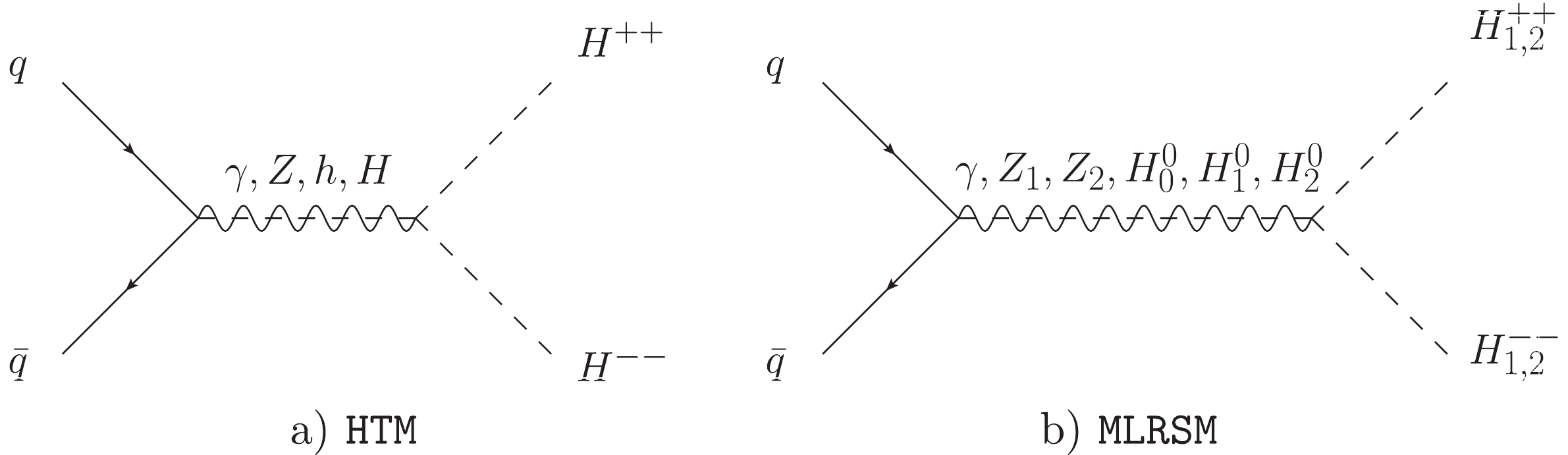
Figure 3. Feynman diagrams for the doubly charged scalar particles' pair production in proton-proton colliders within the (a)
$ {\texttt{HTM}}$ and (b)${\texttt{MLRSM}}$ models. -
The Yukawa term (A6) includes the
$ H^\pm-l-\nu $ and$ H^{\pm\pm}-l-l $ vertices considered in the previous section. They can contribute to several LFV processes, including radiative decay of charged leptons$ l_i \rightarrow l_j \gamma $ , three body decay of charged leptons$ l_i \rightarrow l_j l_k l_l $ , and μ-to-e conversion in nuclei$ \mu N \rightarrow e N^* $ . We show the contributing diagrams for the$ {\texttt{HTM}}$ in Fig. 4(a)-(e). In Fig. 4(f) we include the muonium-antimuonium conversion$ \mu^- e^+ \to \mu^+ e^- $ . Corresponding limits on the$ H^{\pm \pm} $ parameters are given in Table 2. Table 3 shows the relevant SM processes: Møller scattering$ e^- e^- \to e^- e^- $ , Bhabha scattering$ e^+ e^- \to e^+ e^- $ , and the anomalous magnetic moment of the muon$ (g-2)_{\mu} $ , from which useful limits on the$ H^{\pm \pm} $ parameters are also derived. These processes have been discussed in the context of the$ {\texttt{HTM}}$ in many works [33, 89-95]). The branching ratios (BRs) in Table 2 depend on the charged scalar masses and the Yukawa couplings$ {\cal{Y}}_{\ell\ell'} $ , defining the allowed space of mass and coupling parameters for charged scalars.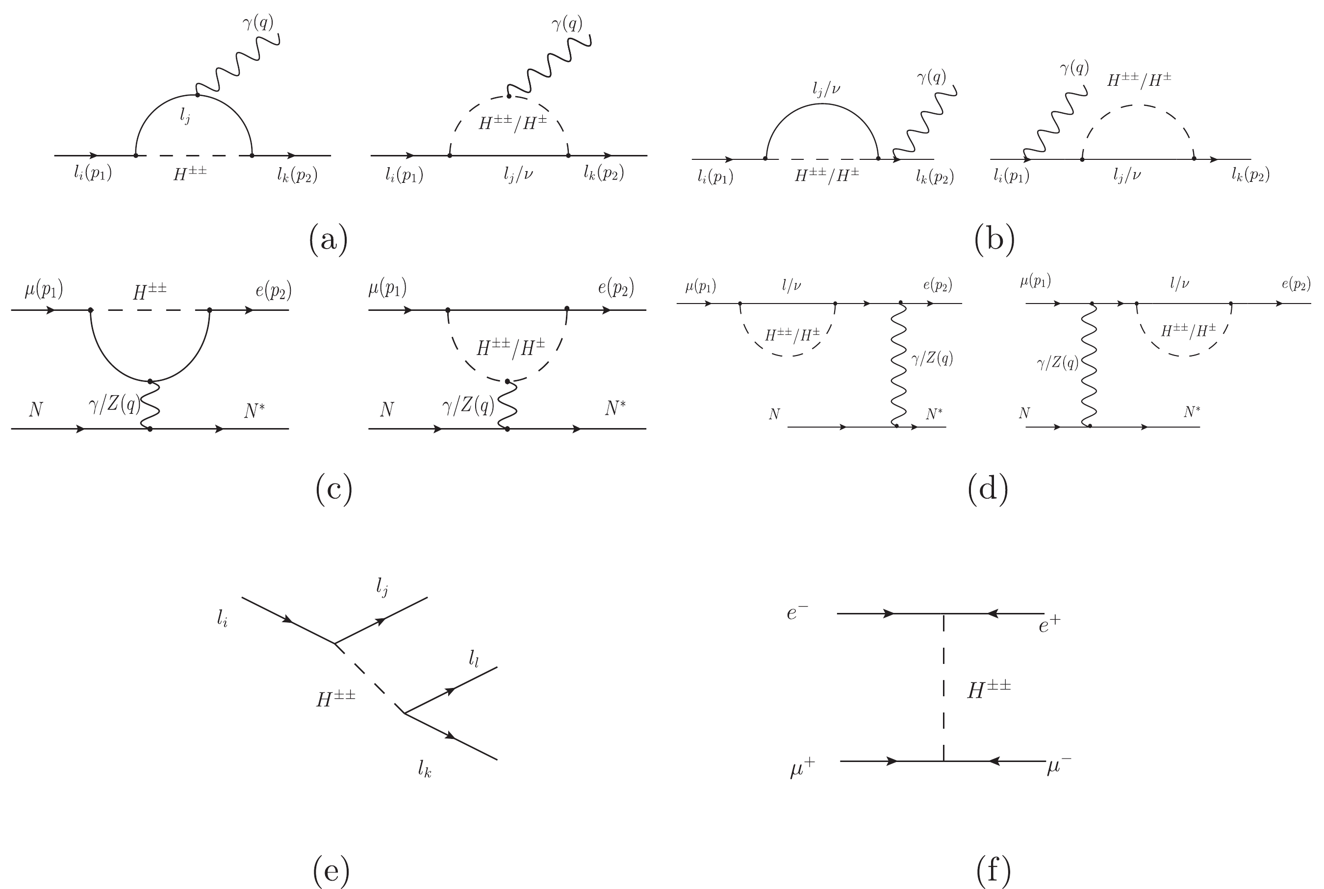
Figure 4. Feynman diagrams representing the contributions to various lepton flavor violating processes mediated by charged scalars in the
$ {\texttt{HTM}}$ . (a) and (b) represent the radiative decay$l_i\to l_j\gamma$ ; (c) and (d) correspond to μ to e conversion. The contribution of three body decay of leptons is shown in diagram (e), and diagram (f) represents muonium-antimuonium conversion.Process Present limits Future limits LFV processes BR( $\mu \rightarrow e \gamma$ )

4.2× $10^{-13}$ 

[105] 6.0× $10^{-14}$ 

[106] BR( $\tau \rightarrow e \gamma$ )

3.3× $10^{-8}$ 

[107] 1.0× $10^{-8}$ 

[108] BR( $\tau \rightarrow \mu \gamma$ )

4.4× $10^{-8}$ 

[107] 3.0× $10^{-9}$ 

[109] BR( $\mu \rightarrow e e e$ )

1.0× $10^{-12}$ 

[110] $\sim 10^{-16}$ 

[111] BR( $\tau \rightarrow e e e$ )

2.7× $10^{-8}$ 

[112] 5.0× $10^{-10}$ 

[108] BR( $\tau \rightarrow \mu \mu \mu$ )

2.1× $10^{-8}$ 

[112] 4.0× $10^{-10}$ 

[108] BR( $\tau^- \rightarrow \mu^+ e^- \mu^-$ )

2.7× $10^{-8}$ 

[112] 5.0× $10^{-10}$ 

[108] BR( $\tau^- \rightarrow \mu^+ e^- e^- $ )

1.5× $10^{-8}$ 

[112] 3.0× $10^{-10}$ 

[108] BR( $\tau^- \rightarrow e^+ \mu^- \mu^-$ )

1.7× $10^{-8}$ 

[112] 3.0× $10^{-10}$ 

[108] BR( $\tau^- \rightarrow e^+ e^- \mu^- $ )

1.8× $10^{-8}$ 

[112] 3.0× $10^{-10}$ 

[108] R( $\mu N \rightarrow e N^*$ )

7.0× $10^{-13}$ (for Au)

[113] 2.87× $10^{-17}$ (for Al)

[114] $\mu^+ e^- \: \to \: \mu^- e^+$ 

$ \sqrt{{\cal{Y}}_{ee}\cdot{\cal{Y}}_{\mu\mu}} < \dfrac{0.44 \cdot M_{H^{\pm\pm}}}{10^3 \;{\rm{GeV}}} $ 

[115] Table 2. Current and future limits on processes with doubly charged scalar contributions and LFV processes (90% CL).
Process Present limits SM processes $e^+ e^- \to l^+ l^-$ (LEP)

$|{\cal{Y}}_{ee}| \leqslant \dfrac{\sqrt{4\pi} \: M_{H^{\pm\pm}}}{8.7 \times 10^3 \: \;{\rm{GeV}}}$ 

[116] $|{\cal{Y}}_{e\mu}| \leqslant \dfrac{1}{\sqrt{2}} \dfrac{\sqrt{4\pi} \: M_{H^{\pm\pm}}}{12.2 \times 10^3 \: \;{\rm{GeV}}}$ 

[116] $|{\cal{Y}}_{e\tau}| \leqslant \dfrac{1}{\sqrt{2}} \dfrac{\sqrt{4\pi} \: M_{H^{\pm\pm}}}{9.1 \times 10^3 \: \;{\rm{GeV}}}$ 

[116] $e^- e^- \to e^- e^- ({\rm M} \varnothing {\rm {LLER}})$ 

$|{\cal{Y}}_{ee}| \leqslant \dfrac{M_{H^{\pm\pm}}}{3.7 \times 10^3 \: \;{\rm{GeV}}}$ 

[117] $(g-2)_\mu$ 

$\Delta a_\mu = (29.3 \pm 9.0) \times 10^{-10}$ 

[118] Table 3. Current limits on SM processes with doubly charged scalar contributions (95% CL).
The radiative decays
$ l_i\to l_j \gamma $ and the μ-to-e conversion process mediated by doubly and singly charged scalar bosons originate from the following Lagrangian [96]$\begin{aligned}[b] {\cal{L}}\subset& -\frac{4 e G_F}{\sqrt{2}} m_l A_R(q^2)\; \bar{l}^{'} \sigma^{\nu\mu} P_R\; l\; F_{\mu\nu}\\&-\frac{e^2 G_F}{\sqrt{2}} A_L(q^2)\; \bar{l}^{'}\gamma^\nu P_L l\sum\limits_{q = u,d}q_Q \bar{Q}\gamma_\nu Q +{\rm h.c.} \end{aligned}$

(5) The BRs depend on the form factors
$ A_L $ and$ A_R $ , the actual forms of which depend on Higgs scalar contributions to the considered processes. For the doubly charged scalar, there are four relevant diagrams, as shown in Fig. 4(a) and (b). The amplitude for$ H^{\pm \pm} $ for the first two diagrams in Fig. 4(a), at the leading order of the doubly charged scalar mass, is$ \begin{aligned}[b] {\cal{M}}_{M_{H^{\pm\pm}}}^I \subset& -\frac{({\cal{Y}}^*)_{ei} ({\cal{Y}})_{\mu i}\gamma_{\mu} P_L}{128\pi^2}\Big(\frac{2}{\epsilon}+\log\frac{4\pi\mu^2}{M_{H^{\pm\pm}}^2}\Big)\\& +\frac{({\cal{Y}}^*)_{ei} ({\cal{Y}})_{\mu i}\gamma_{\mu} P_L}{64\pi^2}\Big(-\frac{1}{4}-\frac{r}{36}+\frac{s_i}{2}+\frac{r}{6}f(r,s_i)\Big) \end{aligned} $

(6) $ \begin{aligned}[b]& +\frac{({\cal{Y}}^*)_{ei} ({\cal{Y}})_{\mu i} P_L}{384\pi^2 M_{H^{\pm\pm}}^2}\Big[\Big(-\frac{5}{6}+{f(r,s_i)}\Big)(\not\!\!{p}_1\gamma_{\mu} \not\!\!{p_1}+\not\!\!{p_2}\gamma_{\mu} \not\!\!{p}_2) \\& +\Big(\frac{1}{6}+{f(r,s_i)}\Big)(\not\!\!{p}_1\gamma_{\mu} \not\!\!{p}_2)+\Big(\frac{17}{6}-{f(r,s_i)}\Big)(\not\!\!{p}_2\gamma_{\mu} \not\!\!{p}_1)\Big] \\&-\frac{({\cal{Y}}^*)_{ei} ({\cal{Y}})_{\mu i} P_R}{1152\pi^2M_{H^{\pm\pm}}^2}\Big({\not\!\!{p}_1 p_{1\mu}}+{5\not\!\!{p}_1 p_{2\mu}}+5{\not\!\!{p}_2 p_{1\mu}}+{\not\!\!{p}_2 p_{2\mu}}\Big), \end{aligned} $

(6) where
$\begin{aligned}[b]f(r,s_i) =& \dfrac{4 s_i}{r}+\log(s_i)+\Bigg(1-\dfrac{2 s_i}{r}\Bigg) \sqrt{1+\dfrac{4s_i}{r}} \\&\times\log \Bigg(\dfrac{\sqrt{r}+\sqrt{r+4s_i}}{\sqrt{r}-\sqrt{r+4s_i}}\Bigg) ,\; r = \dfrac{-q^2}{m_{H^{\pm\pm}}^2}{,} s_i = \dfrac{m_i^2}{m_{H^{\pm\pm}}^2}\end{aligned}$

μ is a mass parameter introduced in dimensional regularization,
$ \epsilon = 4-D $ , and D is the dimension.The contribution from the other two diagrams in Fig. 4(b), mediated by the doubly charged scalar boson, is
$ \begin{aligned}[b] {\cal{M}}_{M_{H^{\pm\pm}}}^{II} \subset& \frac{({\cal{Y}}^*)_{ei} ({\cal{Y}})_{\mu i}\gamma_{\mu} P_L}{128\pi^2}\Big(\frac{2}{\epsilon}+\log\frac{4\pi\mu^2}{M_{H^{\pm\pm}}^2}\Big)\\&+\frac{({\cal{Y}}^*)_{ei} ({\cal{Y}})_{\mu i}\gamma_{\mu} P_L}{128\pi^2}\Big(\frac{1}{2}+\frac{s_e+s_{\mu}}{3}-{s_i}\Big)\\&+\frac{({\cal{Y}}^*)_{ei} ({\cal{Y}})_{\mu i} P_R}{384\pi^2M_{H^{\pm\pm}}^2}\Big({\not\!\!{p}_2\gamma_{\mu} \not\!\!{p}_1}\Big). \end{aligned} $

(7) By adding (6) and (7), we can see that the final contribution is finite, and after doing some algebra, the contribution of the doubly charged scalar form factors can be written in a more compact way
$ \begin{aligned}[b] {\cal{M}}_{M_{H^{\pm\pm}}} \subset& -\frac{({\cal{Y}}^*)_{ei} ({\cal{Y}})_{\mu i} }{192\pi^2 M_{H^{\pm\pm}}^2}f(r,s_i)(q^2 \gamma_{\mu}-q_{\mu} q_\nu \gamma^\nu)P_L \\ &-\frac{({\cal{Y}}^*)_{ei} ({\cal{Y}})_{\mu i}}{192\pi^2 M_{H^{\pm\pm}}^2}(m_e P_L i\sigma_{\mu\nu}q^\nu+m_{\mu} P_R i\sigma_{\mu\nu}q^\nu). \end{aligned} $

(8) In a similar way, the contributions from diagrams mediated by singly charged scalar bosons can be computed, and the total amplitude in the
$ {\texttt{HTM}}$ can be written as$ \begin{aligned}[b] {\cal{M}}_{\rm HTM} \subset& -\frac{({\cal{Y}}^*)_{ei} ({\cal{Y}})_{\mu i} }{192\pi^2 }\Big(\frac{1}{12 M_{H^{\pm}}^2 }+\frac{f(r,s_i)}{M_{H^{\pm\pm}}^2}\Big)(q^2 \gamma_{\mu}-q_{\mu} q_\nu \gamma^\nu)P_L \\&-\frac{({\cal{Y}}^*)_{ei} ({\cal{Y}})_{\mu i}}{192\pi^2 }\Big(\frac{1}{8 M_{H^{\pm}}^2}+\frac{1}{M_{H^{\pm\pm}}^2}\Big)(m_e P_L i\sigma_{\mu\nu}q^\nu\\&+m_{\mu} P_R i\sigma_{\mu\nu}q^\nu). \end{aligned} $

(9) Matching Eq. (9) to Eq. (5), we can extract the form of the
$ A_L(A_R) $ form factors and compute the analytic formulas for the radiative decays and μ-to-e conversion processes. The final analytic formula for the considered LFV processes are gathered in the Appendix.If the massive neutrinos couple to leptons and are of Majorana type, the lepton number can be violated by two units,
$ \Delta L = 2 $ . This leads to the neutrinoless double beta decay$ \beta\beta 0 \nu $ process [97, 98]; as it has not been observed so far, this puts a constraint on the model parameters. This process has been analyzed within the$ {\texttt{HTM}}$ in [99], where the non-standard contribution is negligibly small.Above, we have discussed LFV processes that have not been observed so far, leading to stringent bounds on BSM physics and parameters. Useful information about limits on the BSM physics can be also obtained by exploring observed SM processes and analyzing experimental results and SM predictions. One of such finite processes is the Bhabha scattering present in electron-positron collisions, which serves as a calibration method for colliders, as it is a QED dominated t-channel process; see Section II and Figs. 1-2 in [100]. The LEP data [101] set a lower limit on
$ H^{\pm\pm} $ , namely$ {\cal{Y}}_{\ell\ell'} \geqslant 10^{-7} $ (to ensure$ H^{\pm\pm} $ decay before entering the detector).Another SM experiment that seems to provide a promising signature of the BSM physics is the observed excess in the anomalous magnetic moment of the muon
$ (g-2)_{\mu} $ . There is a lasting discrepancy of greater than$ 3\sigma $ in the measurement of$ (g-2)_{\mu} $ , considering the corresponding SM value [102]. At present, the deviation, as given by PDG, is [103]:$ \Delta a_{(g-2)_{\mu}} \equiv a_{\mu}^{\rm{exp}} - a_{\mu}^{\rm{SM}} = 268(63)(43) \times 10^{-11}. $

(10) The experimental limits for Bhabha, Møller, and
$ (g-2)_{\mu} $ SM processes are collected in Table 3. Charged scalars can contribute to the$ (g-2)_{\mu} $ at the one-loop level. There are many studies of the BSM contribution to$ (g-2)_{\mu} $ in the literature. The contribution from a doubly charged Higgs boson to$ (g-2)_{\mu} $ is discussed in [104] and in the context of the$ {\texttt{HTM}}$ in [90]. The diagrams mediated by singly and doubly charged scalars contributions to$ (g-2)_{\mu} $ are given by Fig. 4 (a) and (b), where both$ l_i, l_j $ are μ (muons). The contributions of singly and doubly charged scalar bosons to$ (g-2)_{\mu} $ amount to a negative number [57], and the$ (g-2)_{\mu} $ anomaly is hard to explain with$ H^{\pm \pm} $ . However, it is worth mentioning that the observed anomaly is an open problem, as there are still some discrepancies among various low-energy experiments [102]. -
From Eq. (3), we can see that the
$ H^{\pm\pm}-l-l' $ couplings depend on the neutrino oscillation parameters, neutrino hierarchy, and the lightest neutrino mass. Details of studies for the$ {\texttt{HTM}}$ model are thus very sensitive to the neutrino oscillation data, as discussed in [33] and [54, 85, 119]. In our analysis, the following standard parametrization of the$ V_ {\texttt{PMNS}}$ matrix is used:$ V_{{\texttt{PMNS}}} = \left[ {\begin{array}{*{20}{c}} {{c_{12}}{c_{13}}{{\rm e}^{{\rm i}{\alpha _1}}}}&{{s_{12}}{c_{13}}{{\rm e}^{{\rm i}{\alpha _2}}}}&{{s_{13}}{{\rm e}^{-{\rm i}{\delta _{CP}}}}}\\ {( - {s_{12}}{c_{23}} - {c_{12}}{s_{23}}{s_{13}}{{\rm e}^{{\rm i}{\delta _{CP}}}}){{\rm e}^{{\rm i}{\alpha _1}}}}&{({c_{12}}{c_{23}} - {s_{12}}{s_{23}}{s_{13}}{{\rm e}^{{\rm i}{\delta _{CP}}}}){{\rm e}^{{\rm i}{\alpha _2}}}}&{{s_{23}}{c_{13}}}\\ {({s_{12}}{s_{23}} - {c_{12}}{c_{23}}{s_{13}}{{\rm e}^{{\rm i}{\delta _{CP}}}}){{\rm e}^{{\rm i}{\alpha _1}}}}&{( - {c_{12}}{s_{23}} - {s_{12}}{c_{23}}{s_{13}}{{\rm e}^{{\rm i}{\delta _{CP}}}}){{\rm e}^{{\rm i}{\alpha _2}}}}&{{c_{23}}{c_{13}}} \end{array}} \right], $

(11) where
$ s_{ij} $ and$ c_{ij} $ denote$ \sin({\theta_{ij}}) $ and$ \cos({\theta_{ij}}) $ , respectively. Table 4 shows global neutrino fits at the$ 2\sigma $ C.L. for neutrino parameters that are used in the present analysis for two mass orderings, defined as:Normal hierarchy (NH) Inverted hierarchy (IH) Best fit (bf): σ bf $\pm 1\sigma$ 

bf $\pm 2\sigma$ 

Best fit (bf): σ bf $\pm 1\sigma$ 

bf $\pm 2\sigma$ 

$\sin^2{\theta_{12}}$ 

0.310 $+0.013$ 

$-0.012$ 

0.298÷0.323 0.286÷0.336 0.310 $+0.013$ 

$-0.012$ 

0.298÷0.323 0.286÷0.336 $\sin^2{\theta_{23}}$ 

0.558 $+0.020$ 

$-0.033$ 

0.525÷0.578 0.492÷0.598 0.563 $+0.019$ 

$-0.026$ 

0.537÷0.582 0.511÷0.601 $\sin^2{\theta_{13}}$ 

0.02241 $+0.00066$ 

$-0.00065$ 

0.02176÷0.02307 0.02111÷0.02373 0.02261 $+0.00067$ 

$-0.00064$ 

0.02197÷0.02328 0.02133÷0.02395 $\delta_{CP}[^o]$ 

222 $+38$ 

$-28$ 

194÷260 166÷298 285 $+24$ 

$-26$ 

259÷309 233÷333 $\dfrac{\Delta m^2_{21}}{10^{-5}\; {\rm{eV}}^2}$ 

7.39 $+0.21$ 

$-0.20$ 

7.19÷7.60 6.99÷7.81 7.39 $+0.21$ 

$-0.20$ 

7.19÷7.60 6.99÷7.81 $\dfrac{\Delta m^2_{3l}}{10^{-3}\; {\rm{eV}}^2}$ 

+2.523 $+0.032$ 

$-0.030$ 

2.463÷2.527 2.463÷2.587 −2.509 $+0.032$ 

$-0.030$ 

−2.539÷−2.477 −2.569÷−2.445 Table 4. Neutrino oscillation data; notations as in [120].
$\Delta m_{ij}^2 = m_i^2 - m_j^2$ . Depending on the hierarchy, for atmospheric nutrino oscillations, either$\Delta m_{3l}^2 = \Delta m_{31}^2 > 0$ (NH) or$\Delta m_{3l}^2 = \Delta m_{32}^2 < 0$ (IH).$\begin{array}{*{20}{c}} {{\rm{Normal}}\; {\rm{mass}}\; {\rm{hierarchy:}}}&{{\rm{Inverted}}\; {\rm{mass}}\; {\rm{hierarchy:}}}\\ {\begin{array}{*{20}{l}} {{m_{{\nu _1}}} = {m_{{\nu _0}}},}\\ {{m_{{\nu _2}}} = \sqrt {m_{{\nu _0}}^2 + \Delta m_{21}^2} ,}\\ {{m_{{\nu _3}}} = \sqrt {m_{{\nu _0}}^2 + \Delta m_{31}^2} ,} \end{array}}&{\begin{array}{*{20}{l}} {{m_{{\nu _1}}} = \sqrt {m_{{\nu _0}}^2 - \Delta m_{21}^2 - \Delta m_{32}^2} ,}\\ {{m_{{\nu _2}}} = \sqrt {m_{{\nu _0}}^2 - \Delta m_{32}^2} ,}\\ {{m_{{\nu _3}}} = {m_{{\nu _0}}},} \end{array}} \end{array}$

(12) where
$ \Delta m_{ij}^2 = m_i^2-m_j^2 $ .Concerning the Dirac CP-phase
$ \delta_{CP} $ , the global fits indicate preference for non-zero values. Recent T2K results confirm this tendency, and the$ 2\sigma $ range of the Dirac phase considered here covers well the best fit values given in [121]. In our analysis, we choose$ \delta_{CP} $ data, as given in Table 4. There is no direct limit on the Majorana phases$ \alpha_1 $ and$ \alpha_2 $ . However, in some studies, there are predictions using the neutrinoless double beta decay, e.g., [122]. There is no bound on the individual masses of neutrinos from the oscillation data. Therefore, the lightest neutrino mass$ m_{\nu_0} $ is a free parameter, and the other two masses are determined through (12). Also, there are limits on the sum of three neutrino masses from various experiments: from the tritium decay [123] or the neutrinoless double beta decay [124], the sharpest limit comes from astrophysics and cosmology [125]$ \Sigma \equiv \sum\limits_{i = i}^3 m_{\nu_i} \leqslant 0.23 \; {\rm{eV}}. $

(13) These limits set the upper bound on the lightest neutrino mass [126, 127], and the present experimental data give
$ {m_{{\nu _0}}} = \left\{ {\begin{array}{*{20}{c}} {0.071\;{\rm{eV}},}&{{\rm{NH}},}\\ {0.066\;{\rm{eV}},}&{{\rm{IH}}.} \end{array}} \right. $

(14) -
As mentioned in the introduction, the additional scalar triplet contributes to the ρ parameter. It can be defined either through a relation among massive SM gauge bosons Z and W and the Weinberg mixing angle or by relations among gauge couplings [128]. In the
$ {\texttt{HTM}}$ , at the tree level, ρ can be written as [129]:$ \rho = \frac{1+2\dfrac{v_{\Delta}^2}{v_\Phi^2}}{1+4\dfrac{v_{\Delta}^2}{v_\Phi^2}} \,. $

(15) The experimental limit on the ρ parameter [130],
$ \rho^{\rm exp} = 1.00037 \pm 0.00023, $

(16) puts the upper bound on the triplet VEV
$ v_{\Delta} $ .Taking
$ \sqrt{v_\Phi^2 +2 v_{\Delta}^2} = v = (\sqrt{2}G_F)^{-\frac{1}{2}} $ [131, 132], where$ G_F $ is the Fermi coupling constant$ 1.1663787(6) $ $ \times $ $ 10^{-5} $ $ {\rm{GeV}}^{-2} $ [103], we obtain$ v_{\Delta} \leqslant 1.7\;{{\rm{GeV}}}, $

(17) for
$\rho^{\rm exp}$ , within$ 2\sigma $ deviations. Note that the limit on$ v_{\Delta} $ can not be obtained for$\rho^{\rm exp}$ within$ 2\sigma $ deviation. This is connected to the fact that relation (16) makes sense only for$\rho^{\rm exp}\leqslant 1$ ; otherwise,$ v_{\Delta} $ becomes a complex number. The following section demonstrates that other low experimental data are more important, decreasing the scale of$ v_{\Delta} $ in an unambiguous way to the (sub)electronvolt level. -
In this section, we analyze bounds on the triplet VEV
$ v_{\Delta} $ from low and high energy experiments discussed earlier (see Tables 2 and 3). Figure 5 shows excluded regions in the plane of$ v_{\Delta} $ and the$ M_{H^{\pm\pm}} $ parameters' space based on current limits on BRs (for both NH and IH scenarios) for various LFV processes and$ (g-2)_{\mu} $ . The analytic formulas for the relevant quantities are collected in the Appendix. In this analysis, we consider a range of neutrino oscillation parameters of$ 2\sigma $ ; see Table 4. Majorana phases$ \alpha_1 $ and$ \alpha_2 $ are varied in the full range (0,$ 2\pi $ ). We vary the lightest neutrino mass$ m_{\nu_0} $ , keeping the$ \Sigma $ (sum of neutrino masses) limit (13) for both inverted and normal hierarchies. We assume degenerate mass for charged scalar bosons,$ M_{H^{\pm \pm}} = M_{H^\pm} $ , and vary them from$ \sim 500 $ GeV to 1000 GeV ($ M_{H^{\pm\pm}}\lesssim 470 $ is already excluded by the LHC; see Section V and the discussion around Table 9). The shaded regions in Fig. 5 are excluded from the LFV and muon$ (g-2)\mu $ limits.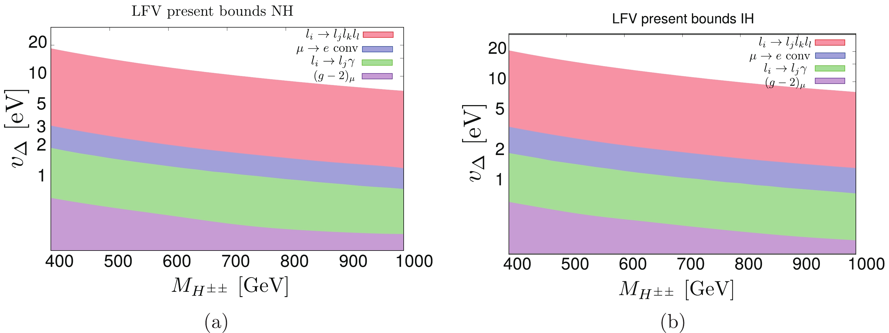
Figure 5. (color online) Plots for
$v_\Delta$ vs.$m_{H^{\pm\pm}}$ using normal and inverted hierarchy data. Shaded regions correspond to the exclusion limits coming from LFV bounds for current data and future sensitivity expectations. The neutrino oscillation data are taken in the$2\sigma$ range. In general, the precision of future experiments (see Table 2) will allow limits for$v_\Delta$ that are one order of magnitude better.BR ll ee $e\mu$ 

μμ 0.01 − 249.2 216.3 309.7 0.02 − 310.9 300.0 335.7 0.03 − 323.7 316.6 367.5 0.04 − 333.9 329.5 418.2 0.05 − 342.5 339.5 434.1 0.1 473.7 478.5 473.7 480.7 0.2 493.5 613.7 573.1 557.9 0.3 518.1 638.9 648.0 683.4 0.4 645.4 658.4 671.7 714.6 0.5 662.7 691.5 690.0 734.0 0.6 679.6 − − − 0.7 695.6 − − − We use different colors to show the exclusion from the individual LFV processes: radiative decay of leptons (green), three body decay of leptons (red), μ-to-e conversion (blue), and
$ (g-2)_{\mu} $ (violet). The most stringent limit is due to three body decays$ l_i \rightarrow l_j l_k l_k $ , specifically the$ \mu \to eee $ process. We do not find any significant difference between the two neutrino mass hierarchy scenarios, but for low neutrino masses, the radiative decay$ \mu \to e \gamma $ begins to play an important role in the normal hierarchy case (see Table 5). Bounds coming from scattering processes or muonium to antimuonium conversion are at least one order of magnitude smaller than those obtained through$ (g-2)_{\mu} $ calculation and are not included in these plots.$\alpha_1$ 

$\alpha_2$ 

NH IH $m_{\nu_0}=0$ 

$m_{\nu_0}=0.01$ 

$m_{\nu_0}=0.071$ 

$m_{\nu_0}=0$ 

$m_{\nu_0}=0.01$ 

$m_{\nu_0}=0.066$ 

0 0 1.04 $\mu \to e \gamma$ 

1.60 $\mu \to e e e$ 

6.45 $\mu \to e e e$ 

3.36 $\mu \to e e e$ 

3.74 $\mu \to e e e$ 

7.47 $\mu \to e e e$ 

0 $\dfrac{\pi}{2}$ 

1.04 $\mu \to e \gamma$ 

1.15 $\mu \to e e e$ 

7.48 $\mu \to e e e$ 

4.92 $\mu \to e e e$ 

4.99 $\mu \to e e e$ 

8.09 $\mu \to e e e$ 

$\dfrac{\pi}{2}$ 

0 1.04 $\mu \to e \gamma$ 

1.04 $\mu \to e \gamma$ 

6.68 $\mu \to e e e$ 

4.92 $\mu \to e e e$ 

5.06 $\mu \to e e e$ 

8.56 $\mu \to e e e$ 

$\dfrac{\pi}{2}$ 

$\dfrac{\pi}{2}$ 

1.04 $\mu \to e \gamma$ 

1.71 $\mu \to e e e$ 

5.61 $\mu \to e e e$ 

3.36 $\mu \to e e e$ 

3.09 $\mu \to e e e$ 

3.15 $\mu \to e e e$ 

Oscillations $\pm 2 \sigma$ 

0.93÷10.31 1.07 $\div$ 11.38

Table 5. Lower bounds on the triplet vacuum expectation value
$v_\Delta$ (in eV) for various values of Majorana phases and doubly charged scalar mass$M_{H^{\pm\pm}} = 700$ GeV. The most strict limit comes from the LFV processes named under the numerical value. The triplet VEV$v_\Delta$ is primarily bounded by experimental limits on$\mu \to eee$ and$\mu \to e\gamma$ dacays. The first four rows present results for the best fit of neutrino oscillation data. The last row shows the range of the lowest possible$v_\Delta$ for oscillation parameters within the$\pm 2\sigma$ range and Majorana phases within the entire$2\pi$ angle. All values in the table are in eV.In Table 5, we collect the lower limits of
$ v_{\Delta} $ in eV for various values of Majorana phases and the lightest neutrino mass, assuming$ m_{H^{\pm\pm}} = 700 $ GeV. The process that leads to the strongest limit is given below the numerical values. For further analysis and the$ {\texttt{HTM}}$ benchmark point, we take$ v_{\Delta} = 15 $ eV. -
We consider a left-right symmetric model based on the
$ SU(2)_L \otimes SU(2)_R \otimes U(1)_{B-L} $ gauge group [28, 36-38, 40] in its most restricted form, the so-called Minimal Left-Right Symmetric Model ($ {\texttt{MLRSM}}$ ), which contains a bidoublet Φ and two (left and right) triplets$ \Delta_{L,R} $ [29, 38, 39, 87]; see the Appendix for details. -
The heavy sector of the model is triggered by VEV
$ v_R $ connected with the Higgs triplet$ \Delta_{R} $ . All new gauge and scalar bosons are proportional to$ v_R $ , and$ v_R \gg \kappa $ , where κ is a VEV related to the scale of the SM spontaneous symmetry breaking and to the SM gauge bosons$ W_1, Z_1 $ ,$ \kappa\; \simeq\; 246 $ GeV; see Eq. (A18).Using the relation between the heavy charged gauge boson mass and the
$ SU(2)_R $ triplet$ {\texttt{VEV}}$ $ v_R $ $ M_{W_2}^2 \simeq \frac{g^2 \: v_R^2}{2} \qquad \Rightarrow \qquad M_{W_2} \simeq 0.47 \; v_R, $

(18) we can find the parameter space for
$ v_R $ and heavy neutrino masses. In the last few years, the LHC has markedly constrained the possible$ v_R $ scale by exploiting different channels where$ W_2 $ plays a crucial role, e.g., where$ W_2 $ decays to two jets [133], two jets and two leptons [134], and top-bottom quarks [135]. The following bounds on$ M_{W_2} $ have been obtained: (i) ATLAS - 3.6 TeV (2017) [133]; 4.8 TeV (e-channel) and 5 TeV (μ-channel) for$ M_{N} \in [0.4,0.5] $ TeV (2019) [136]; (ii) CMS -$ 4.4 $ TeV (2018) [134], assuming that$SU(2)_{R}$ gauge coupling$ g_L $ equals the$ SU(2)_{L} $ coupling$ g_R $ . These bounds can be relaxed without such an assumption [137-140]. The CMS experimental data based on the$ pp \to lljj $ process are presented as the$ M_{W_2}-M_{N} $ exclusion plots; see Fig. 6 in [134] and Fig. 7 in [141]. For convenience, we repeat them here in Fig. 6. We use these data and analogous data from the ATLAS collaboration [142], leading to restrictions on the t-channel in Fig. 8 and the final signals presented in Section V.E.
Figure 6. (color online) Upper limit on the
$pp \to lljj$ cross section for various$M_{W_R} \equiv M_{W_2}$ and$M_{N_R} \equiv M_N$ mass hypotheses, for the electron (a), muon (b), and taon (c) channels. The thin-dotted (blue) curves in Fig. a) and b) indicate the region in ($M_{W_2}$ ,$M_{N_i}$ ) parameter space that is expected to be excluded at 68%$ {\texttt{CL}}$ [134, 141].As assumed in Fig. 6, we take
$ M_{W_2} \geqslant M_N $ and a correlation between the masses that are proportional to$ v_R $ [56, 143]. Note that most of the experimental LHC analyses are based on simplified scenarios where heavy neutrinos are mass degenerate with diagonal mixings and where CP-violating effects are not taken into account. However, the CP-parities of neutrinos can be different, leading to destructive interference effects and relaxing limits on the$ v_R $ scale; see [144-146].A simultaneous fit to the SM low energy charged and neutral currents sets a rather weak bound on
$ M_{W_2} $ and thus$ v_R $ , namely$ M_{W_2}>715 $ GeV [103, 144]. However, there are additional restrictions for the model parameters coming from radiative corrections. As far as one loop corrections and additional precision constraints on the$ {\texttt{MLRSM}}$ parameters are concerned, there are very few studies based on LR models, i.e., [39, 128, 144, 147] ($ {\texttt{MLRSM}}$ model), and other reports are as follows: [148, 149] (limits on$ W_2 $ mass coming from the$ K_L-K_S $ process (finite box diagrams, renormalization not required)), [150] (LEP physics), and [151-155] (process$ b\to s \gamma $ ). Some interesting results are discussed in [156, 157], where the problem of decoupling of heavy scalar particles in low energy processes is discussed. In [158], it has been shown that low-energy radiative corrections shrink non-standard parameters to very small regions because of correlations among gauge bosons, scalars, and heavy neutrino masses, although there is still a freedom connected among others with the unknown scale$ v_R $ . We assume$ v_R $ and the windows of possible masses of heavy$ {\texttt{MLRSM}}$ particles allowed by low energy analysis [158-162].In addition to experimental limits, because of tree-unitarity and flavor changing neutral current (FCNC) constraints, the scalar potential parameter
$ \alpha_3 $ in Eq. (40) is restricted, and the masses of neutral Higgs bosons$ H_0^0, A^0 $ should be greater than 10 TeV. The lowest limit on the$ v_R $ scale is$ 1.3 \div 6.5 $ TeV [56], depending on the mass scale of$ {\texttt{FCNC}}$ Higgs bosons [163]. Such a relatively low (TeV) scale for the heavy sector is theoretically possible, even if gauge unification ($ {\texttt{GUT}}$ ) is demanded; for a discussion, see [164] and [165]. -
As discussed in previous sections, we assume
$ M_{H^{\pm\pm}_{(1,2)}} = 700 $ GeV. This value will be further justified when the$ H^{\pm \pm} $ decay BRs are discussed in the following sections. Therefore, for substantial$ H^{\pm\pm} $ pair production in$ e^+e^- $ collisions, we need the center of mass energy$ \sqrt{s} $ to be greater than 1 TeV. As discussed in the Introduction, such energies for$ e^+e^- $ colliders are planned presently only at the CLIC. Numerical results for$ \sqrt{s} = 1.5 $ TeV are gathered in Fig. 7 and Fig. 8 for the$ {\texttt{HTM}}$ and$ {\texttt{MLRSM}}$ , respectively.Contributions from scalar particles in Fig. 1 and Fig. 2 (middle diagrams) are negligible in comparison with the diagrams with the intermediate photon and Z bosons; see Table 7. Within the
$ {\texttt{HTM}}$ , the contribution from the heavy neutral scalar$ H^0 $ in the s-channel is negligible, as both$ l-l-H^0 $ and$ H^{++}-H^{–}-H^0 $ vertices are proportional to$ \sin{\alpha} $ ; see Eq. (A10), which is very small [85]. Also, the contribution from the SM Higgs boson in the s-channel is small, i.e., a few orders of magnitude lower than the contribution from the gauge bosons, because of the small Yukawa${e^+}-{e^-}-h$ coupling and heavy boson mass in the propagator. There is a similar situation in the$ {\texttt{MLRSM}}$ . Even though there are some additional possible intermediating particles in the s channel (scalars and the$ Z_2 $ gauge boson; see Fig. 2), they are heavy, and the couplings are small. Large Higgs boson masses in the propagators are proportional to$ v_R $ (see the Appendix). We assume that the masses of both$ H_1^{\pm\pm} $ and$ H_2^{\pm\pm} $ are equal.$ H_0^3 $ does not contribute to the process because the$ H_0^3-H_{1,2}^{\pm\pm}-H_{1,2}^{\pm\pm} $ vertex is proportional to the left-handed triplet VEV$ v_L $ , which is set to zero to preserve the ρ-parameter [166].$\sqrt{s}=1.5$ TeV

Model Process $e^+e^-\to$ 

γ $Z_1$ 

$Z_2$ 

scalars ${\texttt{MLRSM}}$ 

$H_1^{++}H_1^{--}$ 

87% 13% $\ll 1 $ %

$\ll 1 $ %

$H_2^{++}H_2^{--}$ 

90% 10% $\ll 1$ %

$\ll 1$ %

$ {\texttt{HTM}}$ 

$H^{++}H^{--}$ 

88% 12% − $\ll 1$ %

Table 7. Individual s-channel contributions to the doubly charged pair production in electron-positron collision for
$\sqrt{s}=1.5$ TeV c.m. energy (CLIC) in the$ {\texttt{HTM}}$ and${\texttt{MLRSM}}$ models.As discussed in Section II, the t-channel in the
$ {\texttt{HTM}}$ contains the$ e-l'-H^{\pm\pm} $ vertex inversely proportional to$ v_{\Delta} $ in Eq. (3), so this diagram becomes dominant for small$ v_{\Delta} $ . However, it appears that the region where the t-channel can dominate is ruled out by the low energy data and Table 5. The allowed t-channel cross section for$ e^+ e^- \to H^{++} H^{–} $ is a few orders of magnitude lower than that of the s-channel, which is equal to 2.4 fb; see the solid horizontal line in Fig. 7. Regardless of the choice of the neutrino parameters, the entire region where the t-channel is not negligible is excluded.The
$e^+e^- \to H_1^{++} H_1^{–} + H_2^{++} H_2^{--}$ cross section in the$ {\texttt{MLRSM}}$ (see Fig. 2) depends on the right-handed triplet VEV$ v_R $ and heavy neutrino masses. The allowed space for$ M_{W_2}-M_N $ parameters has been considered in Section IV.A and is based on limits on the heavy neutrino masses taken from the LHC CMS and ATLAS data for the$ pp \to lljj $ process [134, 141, 142]. This process is a collider analogue of the neutrinoless double beta decay mediated by a heavy charged boson and heavy Majorana neutrinos, and the cross-sections depend strongly on the masses and CP-parities of heavy neutrinos [145]. As we have CMS and ATLAS results at our disposal, in calculations, we assume$ M_{W_2} > M_N $ with the same CP-parities of heavy neutrinos. In Fig. 8, we vary the$ M_{W_2} $ mass from 600 GeV to 5.5 TeV and the heavy neutrino mass up to 4.8 TeV and take the best fit expected values for the LHC exclusion data.The production through the t-channel is constrained by the Yukawa coupling, Eq.
$ Y_{ee} $ (4). We assume perturbativity of the coupling$ Y_{ee}\sim {{\cal{O}} \left(1 \right)} $ . From$ M_N = \sqrt{2} h_M v_R $ , Eq. (A40), with$ h_M \lesssim 1 $ , we obtain the relation between$ v_R $ and heavy neutrino masses. Because the LHC exclusion plots assume$ M_N < M_{W_2} $ , this condition is fulfilled automatically for the considered parameter space. The most strict limits come from the Bhabha and Møller processes (see Fig. 9), where the doubly charged scalar particles can contribute. In Table 6, we provide the region of physical masses for heavy neutrinos that arise from the discussed low energy LFV constraints.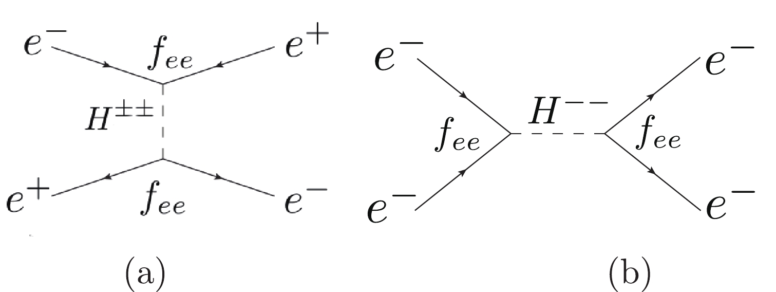
Figure 9.
$e^+ e^- \to e^+ e^-$ (Bhabha) and$e^- e^- \to e^- e^-$ (Møller) processes at the lowest order with doubly charged Higgs bosons.$M_{H_{1,2}^{\pm\pm}}/{\rm{GeV}}$ 

$v_R = 6\;{\rm{ TeV}}$ 

$v_R=15\;{\rm{ TeV}}$ 

700 $M_{N_1} < 803$ GeV

$M_{N_1} < 2007$ GeV

1000 $M_{N_1} < 1147$ GeV

$M_{N_1} < 2867$ GeV

In Fig. 8, the t-channel gray parts of the plotted lines above the long-dashed "Bhabha, Møller" line assigned cross
$ \times $ and plus$ + $ symbols may dominate within the entire region of the$ v_R $ parameter tested by LHC. However, adding the discussed Yukawa constraints on$ H^{\pm \pm} $ couplings gathered in Table 2 and Table 3, this region is eliminated (the corresponding allowed t-channel contributions with red and blue parts of the plotted CMS and ATLAS lines are thickened in Fig. 8). As the Bhabha and Møller processes constrain the t-channel contribution to be below 0.3 fb, together with the LHC constraints, there is a much smaller contribution than the s-channel contribution and the interference effect is small: the total cross section$\sigma_{\rm tot}$ practically corresponds with the s-channel. Even though the mass$ M_{Z_2} $ is a function of$ v_R $ ($ M_{Z_2} \simeq 0.78 \; v_R $ ), the higher resonances are suppressed because the low center of mass energy is too small for them to be observed. For larger$ v_R $ values, we are outside the s-resonance for$ \sqrt{s} = 1.5 $ TeV, and the s-channel contributions are flat and small. For instance, for$ v_R = 6(15) $ TeV, which will be used as a reference value in the next sections for the four lepton final state analysis, this corresponds to$ M_{Z_2} = 4.7 (11.7) $ TeV,$ \sigma_s \simeq 4.6 $ fb. The limits from the muon$ (g-2) $ and$ \mu^+e^-\to\mu^-e^+ $ processes are also taken into account, as the corresponding diagrams contain the$ f_{ee} $ and$ f_{\mu\mu} $ couplings, but they play no significant role. The$ (g-2)_{\mu} $ process restricts the$ f_{\mu\mu} $ coupling; see the Appendix. This affects heavy neutrino mass bounds, and for further calculations, we assume that the maximum$ M_{N_2} = 5 $ TeV, which is safe for the considered values of$ v_R $ (6 and 15 TeV). Unlike the$ {\texttt{HTM}}$ case, the LFV processes do not further restrict the results because we assume the LFV vertices to be negligible with no light-heavy neutrino mixings (see Section VII.C). Taking into account the above constraints, the maximal cross section at the t-channel is$ \sigma_t \sim 0.3 $ fb.All non-standard heavy particle masses are related to the vacuum expectation value of the right-handed triplet; see Appendix A.2 and Eqs. (A22)-(A30). As discussed in [56], the combined effects of relevant Higgs potential parameters and Higgs bosons responsible for FCNC limits regulate the lower limits of heavy gauge boson masses. In Fig. 8, we place only low-energy limits on
$ v_R $ coming from$ (g-2)_{\mu} $ and FCNC. We indicate$ v_R \sim 3.5 $ TeV, which by considering the Higgs boson mass spectrum, Eqs. (A22)-(A28), is the minimal$ v_R $ for FCNC Higgs masses of$ A_1^0,H_1^0 $ scalars at the level of$ \cal{O} $ (10) TeV, and the minimal allowed$ M_{H_{3}^0} $ for$ \alpha_3 $ scalar parameter is less than 16. The mass limit for$ A_1^0,H_1^0 $ at the level of 10 TeV is the lowest limit on FCNC Higgs boson masses [163]; one of the strongest limits has been obtained in [152] ($M_{A_1^0,H_1^0} \geqslant 50 \,{\rm{TeV}}$ ). There are various estimates of the$ v_R $ scale; see also Fig. 6. In addition to the dijet LHC strong limits, there are searches in the one jet and one lepton signal category [136, 167], as well as off-shell$ W_2 $ and$ Z_2 $ channels [168, 169]. These studies confirm that it is not natural to expect$ v_R $ to scale below 3.5 TeV. For these reasons, as pp studies at HL-LHC or future FCC-hh or CEPC colliders offer investigation of heavy BSM states at higher scales, in the following sections, for pp phenomenological studies, we assume a$ v_R $ scale and$ {\texttt{MLRSM}}$ mass benchmarks corresponding to higher$ v_R $ values at the level of 6 and 15 TeV.In Table 7, we show the fractions of dominating s-channel individual contributions to the doubly charged pair production cross section in
$ e^+e^- $ collisions. Individual doubly charged production cross sections are as follows:$\sigma(e^+e^- \rightarrow $ $ H_{1}^{++} H_{1}^{--} ) = 2.46$ fb and$\sigma(e^+e^-\rightarrow H_{2}^{++} H_{2}^{--} ) = 2.15$ fb, which should be compared with$ \sigma(e^+e^-\rightarrow H_{2}^{++} H_{2}^{--} )_{\rm HTM} =$ 2.4 fb in the$ {\texttt{HTM}}$ ; see the solid horizontal line in Fig. 7.Let us proceed to the hadron colliders and pair production of
$ H^{\pm\pm} $ Higgs bosons. Basic tree-level diagrams for the considered models are given in Fig. 3.Figure 10 shows the plot for the
$p p \rightarrow H^{++} H^{--}$ cross sections in both the$ {\texttt{HTM}}$ and$ {\texttt{MLRSM}}$ models. The cross sections are comparable in these models, with slightly larger values for$ {\texttt{MLRSM}}$ . Typically, for$ M_{H_1^{++}} = M_{H_2^{++}} = 1000 $ GeV: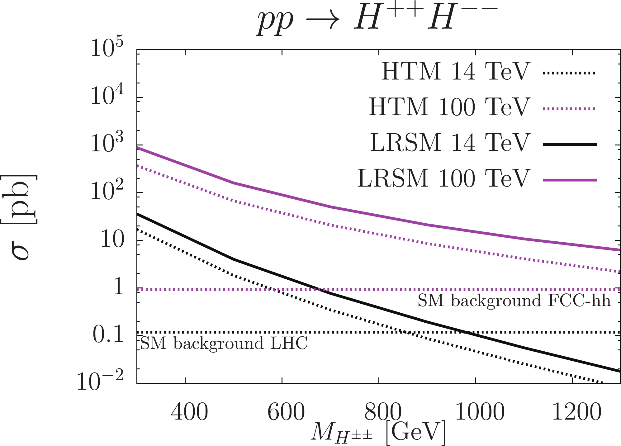
Figure 10. (color online)
$H^{\pm\pm}$ pair production$pp \to $ $ H^{\pm \pm} H^{\pm \pm}$ within the$ {\texttt{HTM}}$ and${\texttt{MLRSM}}$ models for LHC and FCC-hh center-of-mass energies. Horizontal dashed lines give the SM background for the process$pp \to 4l$ , Table 14, with kinematic cuts defined in Section V.D. The QCD NLO$H^{\pm\pm}$ pair production k-factors are taken into account; see the main text.$ \begin{aligned}[b] & \sigma(pp\rightarrow (H_{1}^{++} H_{1}^{--}+H_{2}^{++} H_{2}^{--})\rightarrow {\ell_i}^+{\ell_i}^+{\ell_j}^-{\ell_j}^-)\\ & \quad = 0.063\; (13.02)\; {\rm fb}, \end{aligned}$

(19) for
$ \sqrt{s} = 14(100)\;{\rm{TeV}} $ . The individual$ H_1^{\pm \pm} $ and$ H_2^{\pm \pm} $ contributions to the cross section for$ \sqrt{s} = 14(100)\;{\rm{TeV}} $ are:$ \sigma(pp\rightarrow H_{1}^{++} H_{1}^{--} ) = 0.046\; (7.64)\; {\rm fb}, $

(20) $ \sigma(pp\rightarrow H_{2}^{++} H_{2}^{--} ) = 0.017\; (5.38)\; {\rm fb}, $

(21) $ \sigma(pp\rightarrow H_{}^{++} H_{}^{--} )_{\rm HTM} = 0.044\; (5.13)\; {\rm fb}. $

(22) The
$ {\texttt{HTM}}$ production process is approximately 70% (40%) of that in the$ {\texttt{MLRSM}}$ for$ \sqrt{s} = 14(100) $ TeV. We can see that$\sigma(pp\rightarrow H_{}^{++} H_{}^{--})_{\rm HTM} \simeq \sigma(pp\rightarrow H_{1}^{++} H_{1}^{--})$ , especially for the HL-LHC case. In Table 8, we sum up fractions of particle contributions to the process coming from individual channels. From Eqs. (20)-(22) and Table 8, (i) production of the$ H_2^{\pm \pm} $ is smaller than that of the$ H_1^{\pm \pm} $ , and its contribution increases with c.m. energy; (ii) the γ channel dominates for both$ H_1^{\pm \pm} $ and$ H_2^{\pm \pm} $ pair production at HL-LHC c.m. energies, while for the FCC-hh/CEPC option, the$ Z_2 $ -channel begins to have importance. Because of the shown differences between the$ {\texttt{MLRSM}}$ and$ {\texttt{HTM}}$ models, we can expect a higher number of events for 4-lepton final states in the$ {\texttt{MLRSM}}$ when the masses of doubly charged Higgs bosons are the same. However, this does not have to be the case, as the final results depend strongly on the BRs, which we will consider in the following section.Model Process $pp\to$ 

14 TeV 100 TeV γ $Z_1$ 

$Z_2$ 

scalars γ $Z_1$ 

$Z_2$ 

scalars ${\texttt{MLRSM}}$ 

$H_1^{++}H_1^{--}$ 

63% 36% $< 1$ %

$\ll 1 $ %

43% 27%% 30% $\ll 1$ %

$H_2^{++}H_2^{--}$ 

74% 25% $\sim 1$ %

$\ll 1$ %

68% 9% 23% $\ll 1$ %

$ {\texttt{HTM}}$ 

$H^{++}H^{--}$ 

65% 35% − $\ll 1$ %

62% 38% − $\ll 1$ %

Table 8. Individual channel contributions to the doubly charged pair production
$\sqrt{s}=14$ TeV c.m. energy (HL-LHC) and$\sqrt{s}=100$ TeV c.m. energy (FCC-hh/CEPC) hadron colliders in the$ {\texttt{HTM}}$ and${\texttt{MLRSM}}$ models.The QCD contributions to the doubly charged Higgs boson pair production increase the cross section at the NLO level. The role of the QCD effects in the hadronic processes of
$ H^{\pm \pm} $ pair production has been considered in [54]. A similar situation with a positive contribution of QCD at the NLO and higher levels has also been observed for other processes in models that include triplet Higgs bosons and heavy neutral leptons [54, 170-173]. The corresponding k-factors (which measure the ratios of higher order QCD effects to the tree level cross section) do not change considerably with the$ H^{\pm \pm} $ mass and center of mass energies, i.e., k-factor$ \in (1.15 \div 1.20 $ ). Because of the different ratios of$ H_{1}^{++} $ and$ H_{2}^{++} $ pair production processes (see Eqs. (20)-(22) and Table 8), for$ m_{H^{\pm \pm}} = 1 $ TeV, the k-factor in the$ {\texttt{HTM}}$ is 1.15 and is smaller than the k-factors in the$ {\texttt{MLRSM}}$ , which are$ \simeq 1.6\; (1.85) $ for HL-LHC (FCC-hh/CEPC) center of mass energies. There are various QCD contributions at the NLO level to the considered process, in which the s-channels$ \gamma/Z_1/Z_2 $ dominate over the gluon and photon fusion mechanisms, both for the HL-LHC and FCC-hh/CEPC. Concerning potential contributions beyond the NLO, the$ N^3LL $ terms are found to be approximately three times larger than the NLO terms. However, this is connected primarily to gluon fusion, which is subdominant for the considered$ H_{1}^{++} $ masses in the s-channel [54]. As the doubly charged pair production signals are dominated by the exchange of the SM particles in$ e^+e^- $ collisions (see Table 7), differences between doubly charged pair production signals in the models are small. A better estimation of QCD corrections, evaluating the NNLO terms, would resolve the expected signals better. In the pp collision case, the production difference between the models for the considered benchmark points is much larger. NLO QCD corrections seem to be sufficient to discriminate the models, although we should note that the production difference between the models will decrease above$ v_R = {15} $ TeV, which is the upper limit for the$ v_R $ value considered in the present work. In scenarios with$ v_R > {15} $ TeV, knowledge of NNLO QCD corrections also will be useful in the pp collisions. Anticipating the final four-lepton results, the above conclusions do not change for the considered benchmark points and kinematic cuts. Specifically, the ratios of the$ {\texttt{MLRSM}}$ ($ v_R = 15 $ TeV) to$ {\texttt{HTM}}$ four-lepton signals can be as large as 1.7 (34 and 43) at the$ e^+e^- $ and pp (HL-LHC and CEPC/FCC-hh) colliders, respectively (see the$ 4\mu $ signals in Table 15 and Table 16). Then, the NLO QCD k-factors should be sufficient to distinguish the$ {\texttt{HTM}}$ and$ {\texttt{MLRSM}}$ signals in pp collisions, unless the$ v_R $ scale is too large and the$ {Z_2} $ gauge boson contribution approaches the NNLO QCD level.SM background: $e^+e^- \to 4l$ 

$4e$ 

No cuts: $\sigma = 2.1$ fb

After cuts: $\;\;\sigma = 0.13$ fb, N = 200

$4\mu$ 

No cuts: $\sigma = 0.07$ fb

After cuts: $\;\;\sigma = 0.005$ fb, N = 8

BSM signal: $e^+e^-\to H^{++} H^{--} \to 4l$ 

$ {\texttt{HTM}}$ 

${\texttt{MLRSM}}$ 

NH IH $v_R$ = 6 TeV

$v_R$ = 15 TeV

4e No cuts: 0.19 fb 0.53 fb 0.06 fb 0.924 fb After cuts: 0.02 fb 0.06 fb 0.007 fb 0.113 fb N=30 N=90 N=10 N=169 4μ No cuts: 0.22 fb 0.19 fb 0.06 fb 0.33 fb After cuts: 0.08 fb 0.08 fb 0.03 fb 0.137 fb N=120 N=120 N=38 N=205 Table 15. Four lepton signals at lepton colliders for doubly charged scalar pair production with subsequent decays,
$e^+e^-\to H^{++} H^{--} \to 4l$ for$M_{H^{\pm\pm}}$ = 700 GeV and$\sqrt{s}=1.5$ TeV. To maximize signals in electron and muon channels, we have applied different parameter sets from Table 10 (for the$ {\texttt{HTM}}$ ) and Table 13 (for the${\texttt{MLRSM}}$ ); see the main text for details. "N" estimates the number of final events with assumed luminosity$L=1500$ ${\rm fb}^{-1}$ .SM background: $pp \to 4l$ 

$4e$ 

No cuts: $\sigma = 9.1$ [102.6] fb

After cuts: $\;\;\sigma = 0.0071$ [0.153] fb, N = 28 [3825]

$4\mu$ 

No cuts: $\sigma = 9.1$ [100.6] fb

After cuts: $\;\;\sigma = 0.022$ [0.62] fb, N = 88 [15 167]

BSM signal: $pp \to H^{++} H^{--} \to 4l$ 

$ {\texttt{HTM}}$ 

$ {\texttt{LRSM}}$ 

NH IH $v_R$ = 6 TeV

$v_R$ = 15 TeV

4e No cuts: 0.0038 fb 0.0109 fb 0.0029 fb 0.136 fb [0.39 fb]
[1.11 fb]
[0.87 fb]
[19.6 fb]
After cuts: 0.00032 fb 0.00092 fb 0.00026 fb 0.0116 fb N= 1.3 N= 3.7 N= 1.1 N= 45 [0.020 fb] [0.059 fb] [0.0407 fb] [0.98 fb] [N= 484 ]
[N= 1459]
[N= 1032]
N= [24 492]
4μ No cuts: 0.0092 0.0039 fb 0.0029 fb 0.136 fb [1.086 fb]
[0.48 fb]
[0.87 fb]
[19.6 fb]
After cuts: 0.0031 0.00132 fb 0.001 fb 0.048 fb N= 11.5 N= 5.3 N= 4 N= 180 [0.202 fb] [0.090 fb] [0.181 fb] [3.9 fb] [N= 5057] [N= 2262] [N= 4509] N=[ 97 199] Table 16. Four lepton signals for doubly charged scalar pair production with subsequent decays
$pp \to H^{++} H^{--} \to 4l$ for$M_{H^{\pm\pm}}$ = 1000 GeV and$\sqrt{s}=14\; [100]$ TeV. To maximize signals in electron and muon channels, we have applied different parameter sets from Table 10 (for the$ {\texttt{HTM}}$ ) and Table 13 (for the${\texttt{MLRSM}}$ ); see the main text for details. "N" estimates the number of final events with assumed luminosity$L=4 \;ab^{-1} = 4000$ ${\rm fb}^{-1}$ for HL-LHC [63] and$L=25\; {\rm{ab}}^{-1} = 25000$ ${\rm{fb}}^{-1}$ for FCC-hh [185].To summarize, the QCD contributions to the considered production processes at the NLO level are substantial in both models and must be taken into account in the analysis. To discriminate both models, evalauation of higher order QCD terms may be required for higher
$ v_R $ scales. -
In the
$ {\texttt{HTM}}$ , the doubly charged scalar has nine possible decay channels, depending on the scalar boson mass(i)
$ H^{\pm\pm} \to l_i \: l_j, $ $ i,j = {e,\mu,\tau} $ ,(ii)
$ H^{\pm\pm} \to W^\pm \: W^\pm $ ,(iii)
$ H^{\pm\pm} \to H^\pm \: W^\pm $ ,(iv)
$ H^{\pm\pm} \to H^\pm \: H^\pm $ .In this paper, we focus on the first channel (i) and present a case study for pair production of a doubly charged scalar boson and its subsequent leptonic decays, considered also in [174]. It is a very clean channel, which provides a unique signature for collider signals with a pair of leptons with the same sign [87]. Scenarios (iii) and (iv) require non-degenerate masses for charged scalar particles:
$ M_{H^{\pm\pm}} > M_{H^\pm} + M_W $ and$ M_{H^{\pm\pm}} > 2 M_{H^\pm} $ , respectively.In Fig. 11, we show a variety of BRs as a function of
$ v_{\Delta} $ for various$ H^{\pm \pm} $ decay channels. On the left, we show the following decay modes: leptonic (red),$ W^\pm $ gauge bosons (green), and$ H^{\pm} W^\pm $ (blue). On the right, we provide a variation of leptonic and a pair of gauge boson decay BRs for a degenerate mass of$ H^{\pm\pm} $ . There are two cases here: the solid line is for$ M_{H^{\pm\pm}} = M_{H^{\pm}} = 700 $ GeV, and the dashed line is for a charged scalar boson mass of 300 GeV (this mass is already excluded by the LHC, but we leave it for comparison with previous work; see Fig. 4 in [175]). The shaded region is connected to the lightest neutrino mass and mass hierarchy, within an oscillation parameter range of 2$ \sigma $ . This region does not change the result substantially. The cross-cut point shifts with charged scalar boson mass, but in the interesting mass region, the lepton channel dominates until$ v_{\Delta} $ reaches values in the range of$ 10^4 \div 10^5 $ eV. In Fig. 11(a), we take a mass gap$ M_{H^{\pm\pm}} - M_{H^\pm} = 80 $ GeV; in Fig. 11(b), there is no mass gap and both$ H^{\pm\pm} \to H^\pm W^\pm $ and$ H^{\pm\pm} \to H^\pm H^\pm $ channels are suppressed. It has been shown in [85] and [86] that there are limits on the mass gap$ |M_{H^{\pm\pm}} - M_{H^\pm}| $ to preserve the oblique T-parameter, unitarity, and potential stability condition. For recent work on the vacuum stability conditions of Higgs potentials in various variants of the$ {\texttt{HTM}}$ models, see [176]. From electroweak precision data and limits from the$ h \to \gamma \gamma $ process [83, 84], the dominant contributions occur in the degenerate mass case. Therefore, only leptonic and W gauge boson decay channels are possible. However, the$ H^{\pm\pm}-W^\mp-W^\mp $ vertex is proportional to the triplet VEV$ v_{\Delta} $ , while the Yukawa coupling in the$ H^{\pm\pm}-l^\mp-l^\mp $ vertex is proportional to$\dfrac{1}{v_{\Delta}}$ , so the lepton channels dominate strongly over scenario (ii) for the triplet VEV$ v_{\Delta} < 10^5 $ eV.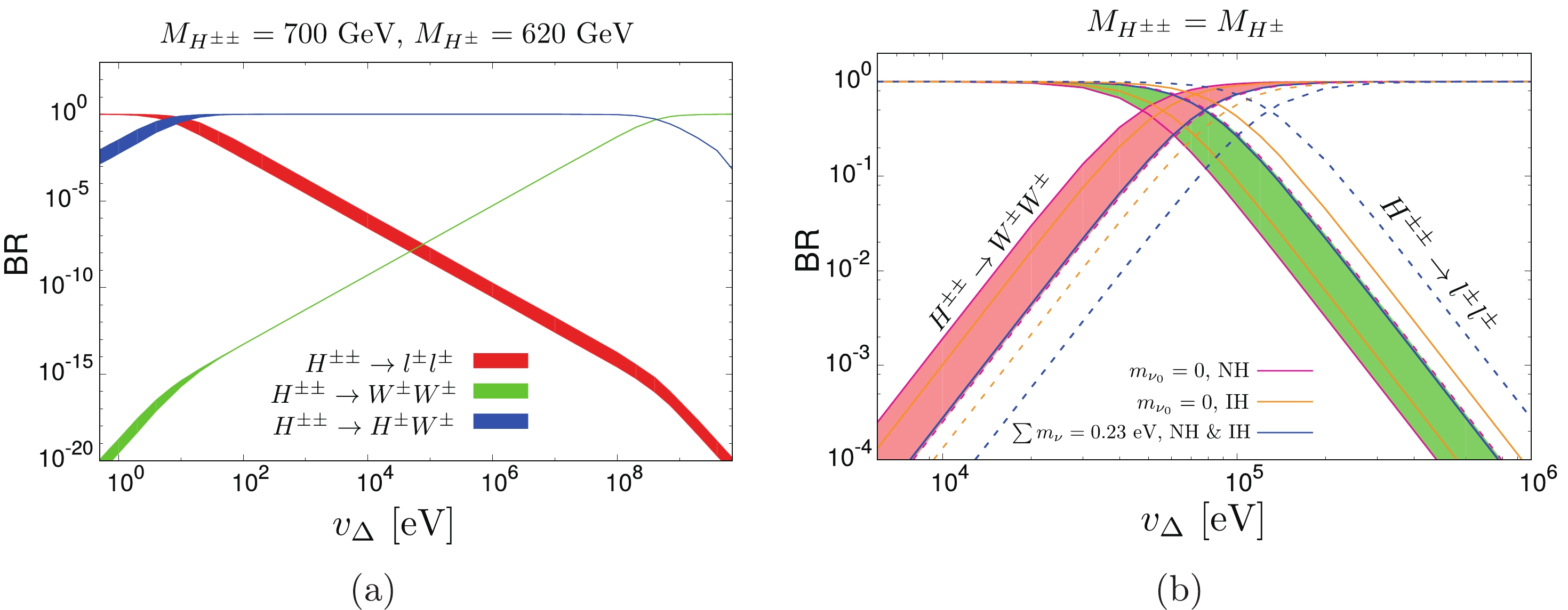
Figure 11. (color online) Branching ratios for
$H^{\pm\pm}$ in the$ {\texttt{HTM}}$ for a non-degenerate case (a) with$m_{H^{\pm\pm}}=700$ GeV and$m_{H^\pm}=620$ GeV and for a degenerate case (b) when$m_{H^{\pm\pm}}=m_{H^{\pm}}=700$ and$300$ GeV are assumed. The shaded regions correspond to IH and NH neutrino mass hierarchies with$m_{\nu_0}$ limited by$\Sigma$ in (13) and$M_{H^{\pm\pm}}=700$ GeV. Dashed lines in case (b) describe the branching ratios for$M_{H^{\pm\pm}} = M_{H^\pm} = 300$ GeV. The oscillation data are in the$2\sigma$ range.For VEV
$ v_{\Delta} $ in a range of eV, the cumulative leptonic channel dominates in that region, regardless of the neutrino masses and oscillation parameters, as well as doubly charged scalar boson masses. Therefore, our final conclusion is that when$ H^\pm W^\pm $ and$ H^\pm H^\pm $ channels are suppressed, the leptonic decays dominate for low$ v_{\Delta} $ .The sharpest limit from ATLAS on
$ M_{H^{\pm\pm}} $ is that the$ {H^{\pm\pm}} $ mass should be larger than 870 GeV for the left-handed triplet doubly charged scalar boson field, assuming the 100% BR for the$ H^{\pm\pm} \to l^\pm l^\pm $ decay ($ l^\pm = e^\pm, \mu^\pm $ ). However, it is possible to decrease the limit to 450 GeV for a 10% leptonic decay BR (see Fig. 13 d in [55]). Conversely, the decays into a τ lepton are not considered in the above analysis. In Table 9, we present BRs for those channels and the result for the ee,$ e\mu $ , and$ \mu\mu $ decays, within the$ \pm 2 \sigma $ range of the oscillation parameter space. For other channels including the τ, we refer to [177]. The strength of lepton decay channels depends strongly on the neutrino masses, their hierarchies, and oscillation parameters. It is possible to find the parameter space where the BR for the particular lepton channel is small, regardless of$ v_{\Delta} $ , even if the cumulative lepton channel dominates over the W boson channel (the relative lepton decay contributions$ \Gamma(H^{\pm\pm}\; \to\; l\; l')/\sum\; \Gamma(H^{\pm\pm}\; \to\; l_i\; l_j) $ do not depend on the triplet VEV$ v_{\Delta} $ ).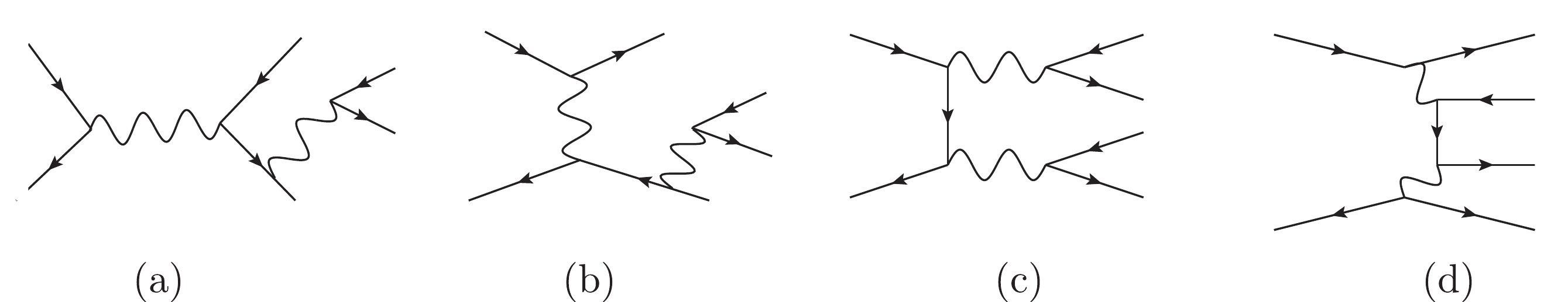
Figure 13. Four lepton background diagrams in electron-positron colliders:
$e^+ e^- \to e^+ e^-$ with FSR$e^+e^-$ pair emission (a) and (b); with$Z/\gamma^*$ production (c); and with multiperipheral processes (d).We combine the data from the LHC limits [55] and neutrino parameters within the
$ \pm 2\sigma $ range given in Table 4 and compute the lowest limit on the doubly charged scalar boson mass②. In Table 9, the BR values that are forbidden by the neutrino oscillation parameters are removed. Another interesting conclusion from this table is that within the$ {\texttt{HTM}}$ , the doubly charged scalar boson cannot be lighter than 473 GeV for the normal neutrino mass scenario (and 518 GeV for the inverted mass hierarchy); see Fig. 12(a). Finally, the lowest mass limit on$ M_{H^{\pm\pm}} $ within the$ {\texttt{HTM}}$ is 473.7 GeV for NH and 645.4 GeV for IH with BR$ (H^{\pm\pm} \to ll') = (\Gamma (H^{\pm\pm} \to e^\pm e^\pm + e^\pm \mu^\pm + $ $ \; \mu^\pm \mu^\pm))/ \Gamma (H^{\pm\pm}\; \to\; \sum\limits_{i,j} l_i^\pm l_j^\pm) \geqslant 0.1 $ and 0.4, respectively, where$ l_{i,j} = e, \mu, \tau $ . The most severe limit at 734 GeVcomes from the same sign muon channel when the BR is 50%.
Figure 12. (color online)
$H^{\pm\pm}$ decay branching ratios, l,$l'$ = e, μ within the$ {\texttt{HTM}}$ model, with corresponding lower limits on the doubly charged scalar particle's masses [55]. Neutrino parameters are within the$\pm 2 \sigma$ range; see Table 4. Solid lines present the result for the best fit of neutrino parameters and particular values of Majorana phases. We have marked the points used for further calculations with$\square$ and$\bullet$ , which satisfy the following conditions:$\bullet$ gives the maximum possible BR for NH and IH cases with$M_{H^{\pm\pm}}$ = 1000 GeV;$\square$ gives lower BR values, which allows for$M_{H^{\pm\pm}} = 700$ GeV.In conclusion, when assuming the complete scenarios with
$ {H^{\pm\pm}} $ decays to all the leptons, still$ M_{H^{\pm\pm}} $ can be relatively light.Our main aim is to analyze the final four lepton (
$ 4l $ ) signals that can be potentially seen at the colliders. The dominant signatures are$ e^+e^+e^-e^- $ and$ \mu^+\mu^+\mu^-\mu^- $ final states within both the$ {\texttt{HTM}}$ and$ {\texttt{MLRSM}}$ models. In the$ {\texttt{MLRSM}}$ , they are not bounded by the neutrino oscillation parameters because the$ H_{1,2}^{\pm\pm}-l-l $ vertex is related to the heavy right-handed neutrino masses and parameters, as discussed in Section A.3. Within the$ {\texttt{HTM}}$ , these$ 4l $ contributions are restricted by the light neutrino oscillation data. Using the BRs shown in Fig. 12, we compute two parameter sets (for normal and inverted hierarchy) for which the BRs for$ e^\pm e^\pm $ and$ \mu^\pm \mu^\pm $ are the highest. We collect the chosen parameters in Table 10. We choose two benchmark masses for the collider analyses:$ M_{H^{\pm\pm}} $ = 700 GeV (which can be probed at very high energies in$ e^+ e^- $ collision, when available; see Section V.A) and$ M_{H^{\pm\pm}} $ = 1000 GeV (this higher mass range can be probed without any problem at the HL-LHC and FCC-hh; see Fig. 10). For the$ e^\pm e^\pm $ decay channel, we chose the same neutrino parameters because within the whole neutrino parameter space,$ M_{H^{\pm\pm}} = 700 $ GeV and$ M_{H^{\pm\pm}} = 1000 $ GeV are not excluded. For the$ \mu^\pm \mu^\pm $ channel, we chose the maximum possible BR for$ M_{H^{\pm\pm}} = 1000 $ GeV and BR = 0.3 for$ M_{H^{\pm\pm}} = 700 $ GeV to keep the bound on the doubly charged scalar particle's mass lower than 700 GeV.$M_{H^{\pm\pm}}$ 

$H^{\pm\pm}\to XX$ 

$ {\texttt{HTM}}$ 

NH IH 700 GeV ( $\square$ )

$ee_{\rm{max}} $ 

$BR < 0.5$ 

BR=0.283 $\alpha_1 = \dfrac{\pi}{2}$ 

BR=0.475 $\alpha_1 = \dfrac{\pi}{2}$ 

$\alpha_2 = \dfrac{\pi}{2}$ 

$\alpha_2 = \dfrac{\pi}{2}$ 

$m_{\nu_0}= 0.071$ eV

$m_{\nu_0}=0$ 

$\mu\mu_{\rm{max}}$ 

$BR < 0.3$ 

BR=0.3 $\alpha_1 = \dfrac{\pi}{2}$ 

BR=0.3 $\alpha_1 = 0$ 

$\alpha_2 = 0$ 

$\alpha_2 = 0$ 

$m_{\nu_0}= 0.025$ eV

$m_{\nu_0}=0.066$ eV

1000 GeV ( $\bullet$ )

$ee_{\rm{max}}$ 

BR=0.283 $\alpha_1 = \dfrac{\pi}{2}$ 

BR=0.475 $\alpha_1 = \dfrac{\pi}{2}$ 

$\alpha_2 = \dfrac{\pi}{2}$ 

$\alpha_2 = \dfrac{\pi}{2}$ 

$m_{\nu_0}= 0.071$ eV

$m_{\nu_0}=0$ 

$\mu\mu_{\rm{max}}$ 

BR=0.438 $\alpha_1 = 0$ 

BR=0.3 $\alpha_1 = 0$ 

$\alpha_2 = 0$ 

$\alpha_2 = 0$ 

$m_{\nu_0}= 0.015$ eV

$m_{\nu_0}=0.066$ eV

Table 10. Chosen parameter set for maximum BRs, i.e., BR
$(H^{\pm\pm} \to ee)$ and BR$(H^{\pm\pm} \to \mu\mu)$ , and for the best fit neutrino parameters in Table 4. Corresponding benchmark points are marked in Fig. 12 (b) and (d) with$\square$ ($M_{H^{\pm\pm}}$ =~700~GeV) and$\bullet$ ($M_{H^{\pm\pm}}$ =1000 GeV). -
Contributing vertices to the non-leptonic decay channels stem from the kinetic term and scalar potential (see Eqs. (19) and (25) in [39]). The relevant decay modes of doubly charged scalar bosons and the respective strength of couplings are given in Table 11. The processes in bold in the table dominate for
$ v_L = \rho_4 = 0 $ and$ \xi \to 0 $ [56, 166, 178]; see the Appendix for details. In addition to the values of vertices, we need to take into account the mass spectrum. To suppress the FCNC processes, some of the neutral scalar particles should be heavier than 10 TeV. As a consequence, the mass of$ H_2^\pm $ should be greater than 10 TeV; see (A22) and (A28). Therefore, we can neglect the$ H_2^{\pm \pm} $ decay to the$ H_2^\pm $ scalar boson for CLIC and LHC energies. From (A22), it is easy to see that the triplet VEV should fulfill an inequality:$ v_R > \sqrt{2} \: 10^3 / \sqrt{\alpha_3} $ [GeV]. Because$ \alpha_3 $ is a quartic coupling (four-scalar interaction), it contributes to the$ 2\to 2 $ scattering, and the unitarity condition requires$ \alpha_3 <8 \pi $ [56]. The triplet VEV$ v_R $ must be higher than$ \sim 2800 $ GeV, which translates to$ M_{W_2} > 1325 $ GeV. Therefore, we can neglect the doubly charged scalar boson pair production with the subsequent decay to the heavy gauge boson pair$ H_2^{\pm\pm} \to W_2^\pm + W_2^\pm $ for energies lower than$ 2 M_{W_2} $ .$H_1^{\pm\pm} \to W_1 + W_1$ 

$\sim \cos^2{\xi}\;v_L$ 

$H_2^{\pm\pm} \to W_1 + W_1$ 

$\sim \sin^2{\xi}\;v_R$ 

$H_1^{\pm\pm} \to W_1 + W_2$ 

$\sim \cos{\xi}\sin{\xi}\;v_L$ 

$H_2^{\pm\pm} \to W_1 + W_2$ 

$\sim \cos{\xi}\sin{\xi}\;v_R$ 

$H_1^{\pm\pm} \to W_2 + W_2$ 

$\sim \sin^2{\xi}\;v_L$ 

${{H}}_{\bf{2}}^{\pm\pm} {\bf{\to}} {{W}}_{\bf{2}} + {{W}}_{\bf{2}}$ 

${\bf{\sim}} {\bf{cos^2}}{{{\xi}}}\;{{v}}_{{R}}$ 

${{H}}_{\bf{1}}^{\pm\pm} {\bf{\to}} {{H}}_{\bf{1}}^\pm + {{W}}_{\bf{1}}$ 

${\bf{\sim}} {\bf{cos}}{{{\xi}}}\;{{g}}_{{L}}$ 

$H_2^{\pm\pm} \to H_2^\pm + W_1$ 

$\sim \sin{\xi}\;g_R$ 

$H_1^{\pm\pm} \to H_1^\pm + W_2$ 

$\sim \sin{\xi}\;g_L$ 

${{H}}_{\bf{2}}^{\pm\pm} {\bf{\to}} {{H}}_{\bf{2}}^\pm + {{W}}_{\bf{2}}$ 

${\bf{\sim}} {\bf{cos}}{{{\xi}}}\;{{g}}_{{R}}$ 

$H_1^{\pm\pm} \to H_1^\pm + H_1^\pm$ 

$\sim \rho_2\;v_L$ 

$H_2^{\pm\pm} \to H_1^\pm + H_1^\pm$ 

$\sim \rho_4\;v_R$ 

$H_1^{\pm\pm} \to H_2^\pm + H_2^\pm$ 

$\sim \rho_4\;v_L$ 

${{H}}_{\bf{2}}^{\pm\pm} {\bf{\to}} {{H}}_{\bf{2}}^\pm + {{H}}_{\bf{2}}^\pm$ 

${\bf{\sim}} {{\rho}}_{\bf{2}}\;{{v}}_{{R}}$ 

$H_1^{\pm\pm} \to H_1^\pm + H_2^\pm$ 

$\sim \kappa_2$ 

$H_{1,2}^{\pm\pm} \to H_{2,1}^{\pm\pm} + H_0^0 $ 

$\sim \rho_4\;v_L$ 

$H_{1,2}^{\pm\pm} \to H_{2,1}^{\pm\pm} + H_1^0 $ 

$\sim \rho_4\;v_L$ 

$H_{1,2}^{\pm\pm} \to H_{2,1}^{\pm\pm} + H_2^0 $ 

$\sim \rho_4\;v_L$ 

$H_{1,2}^{\pm\pm} \to H_{2,1}^{\pm\pm} + H_3^0 $ 

$\sim \rho_4 v_R$ 

$H_{1,2}^{\pm\pm} \to H_{2,1}^{\pm\pm} + A_2^0 $ 

$\sim \rho_4 v_R$ 

Table 11. Doubly charged scalar boson decay channels to scalar and gauge bosons in the
${\texttt{MLRSM}}$ . We have listed all possible vertices, indicating the dominating processes in bold, assuming that the left triplet VEV$v_L$ is equal to zero, keeping in mind experimental limits on the$W_1-W_2$ mixing angle$\xi < 10^{-2}$ [133, 144], and setting the$\rho_4$ parameter to zero [56, 166]. The leptonic decays are analysed separately.In Table 11, we present the other possible decay channels of
$ H_{1,2}^{\pm\pm} $ and the corresponding vertices. Most of them are negligible because of the model's consistency [56, 166], and only the bold decay channels can be substantial. The$ H_{1,2}^{\pm\pm} $ decay to$ H^\pm_2 $ is not possible for CLIC and LHC energies because of the FCNC limits (A28). Vertices contributing to the$ H_{1,2}^{\pm\pm} $ decays to$ W_1 $ ,$ W_2 $ can be large and are included in the analysis leading to the final four lepton signals.Regarding
$ H_1^{\pm\pm} $ , its decay to$ H_1^\pm + W_1^\pm $ is limited by Higgs potential parameters and, as proved analytically in [179], the allowed split$ \Delta M_H = M_{H_1^{\pm\pm}}-M_{H_1^\pm} $ cannot exceed 65.3 GeV.We choose the benchmark points for
$ v_R = 6 $ TeV and$ 15 $ TeV. The first value falls in the energy range of the LHC with$ pp \to W_2 \to l N_l \to ll W_2^* \to ll q\bar{q}' $ , assuming that$ M_{{N}_i} < M_{W_2} $ . Corresponding experimental results can be found in [134, 141]. We assume that the doubly charged scalar masses are degenerate and choose two benchmark points:$ 700 $ GeV and$ 1000 $ GeV. For the$ M_{H_{1,2}^{\pm\pm}} $ = 700 GeV case, we keep the leptonic BR limits as given in Table 9, i.e., BR$ (H^{\pm\pm}_{1,2} \to ee)\; <\; 0.5 $ and BR$ (H^{\pm\pm}_{1,2} \to $ $ \mu\mu)\; <\; 0.3 $ . Table 12 presents the maximum possible BRs for$ M_{H^{\pm\pm}_{1,2}} = 700 $ GeV. For a doubly charged Higgs boson mass of 1000 GeV, there are no relevant experimental limits and the maximum BRs for ee or$ \mu\mu $ decays can reach 100% also in the case of$ {H_{1}^{\pm\pm}} $ . Here, the situation is different from that in the$ {\texttt{HTM}}$ , where upper bounds for the$ {H^{\pm \pm}} $ BRs are given. As discussed in Sections II and III, neutrino Yukawa couplings can be rewritten in terms of oscillation parameters, and$ v_{\Delta} $ and experimental data substantially restrict the possible BRs. In addition, depending on the BR, the lowest limit on the mass of a doubly charged scalar can be obtained. However, in the context of the$ {\texttt{MLRSM}}$ , leptonic branching ratios for$ {H^{\pm \pm}} $ depend in addition on the$ v_R $ scale and heavy neutrino masses and couplings. This freedom makes it possible to reach full leptonic decays for$ M_{H^{\pm \pm}} $ , as given in Table 12 and Table 13.ee μμ $ee+\mu\mu$ 

${\rm{BR}}_{H_1^{\pm\pm}}$ 

0.5 0.3 0.7 ${\rm{BR}}_{H_2^{\pm\pm}}$ 

1.0 0.8 1.0 $M_{H_{1,2}^{\pm\pm}}$ 

${\texttt{MLRSM}}$ 

$H_{1,2}^{\pm\pm} \to$ 

$v_R = 6$ TeV

$v_R = 15$ TeV

700 GeV ${\rm{BR}}^{ee,\mu \mu}_{H_{1,2}^{\pm \pm}}=0.123$ 

$ M_{N_1} = 250$ 

$M_{N_2} = 250$ 

$M_{N_3} = 620$ 

${\rm{BR}}^{ee}_{H_{1,2}^{\pm \pm}}=0.5$ 

${\rm{BR}}^{\mu \mu}_{H_{1,2}^{\pm \pm}}=0.25$ 

$M_{N_1} = 1300$ 

$M_{N_{2,3}}=918$ 

$4e$ 

${\rm{BR}}^{\mu\mu}_{H_{1,2}^{\pm\pm}}=0.3$ 

${\rm{BR}}^{ee}_{H_{1,2}^{\pm\pm}}=0.4$ 

$M_{N_1} = 1300$ 

$M_{N_{2,3}} = 1130$ 

$4\mu$ 

1000 GeV ${\rm{BR}}^{ee,\mu\mu}_{H_{1,2}^{\pm\pm}}=0.123$ 

$M_{N_1} = 250$ 

$M_{N_2} = 250$ 

$M_{N_3} = 620$ 

${\rm{BR}}^{ee}_{H_{1,2}^{\pm\pm}} \sim 1$ 

$M_{N_1} = 2867 $ 

$M_{N_{2,3}}=300$ 

$4e$ 

${\rm{BR}}^{\mu \mu}_{H_{1,2}^{\pm\pm}}\sim 1$ 

$M_{N_2} = 5000$ 

$M_{N_{1,3}} = 300$ 

$4\mu$ 

Table 13.
${\texttt{MLRSM}}$ parameters that maximize separately BR$(H^{\pm\pm}\to ee)$ and BR$(H^{\pm\pm}\to\mu\mu)$ for$v_R=6$ TeV and$v_R=15$ TeV. A scenario with$v_R=6$ TeV has been covered already by the LHC analysis, and the BRs are from Table 12, based on [134, 141]. The heavy neutrino masses for$v_R=6$ TeV fulfill the low energy constraints given in Table 6.$M_{N_1}$ is mostly restricted by the Møller scattering, while$M_{N_2}$ is bounded by$(g-2)_\mu$ .Table 13 shows the chosen, allowed values of heavy neutrino masses for given maximal BRs. They are consistent with assumption
$ M_{W_2} \geqslant M_N $ discussed in Section IV, and a correlation between the masses that are proportional to$ v_R $ [56, 143]. In Section V.B, we have obtained the lowest limits for$ M_{H^{\pm \pm}} $ as a function of the lightest neutrino mass for a given$ H^{\pm \pm} $ BR, arguing that$ M_{H^{\pm \pm}} $ at the level of 700 GeV is still possible within the$ {\texttt{HTM}}$ . The lowest limits on the masses of$ {H^{\pm \pm}_{1,2}} $ Higgs bosons have been obtained in [166] by analyzing restrictions on the scalar potential. Before we present the final results, we will discuss the SM background for the considered leptonic final states. -
We are interested in estimation of the SM background for
$ pp \to l^+ l^- l^+ l^- $ and$ e^+ e^- \to l^+ l^- l^+ l^- $ processes, where$ l^\pm = e^\pm, \mu^\pm $ . The four lepton production at the LHC is discussed in [87, 180]. The most relevant processes that contribute to the background are$ t\bar{t}(Z/\gamma^*) $ and$ (Z/\gamma^*)(Z/\gamma^*) $ production. To optimize the collider non-standard effects (decreasing SM tri- and four-lepton SM background and reducing the efficiency of misidentification of b-jets as leptons), we use the following criteria and selection cuts:C1. Lepton identification criteria: transverse momentum
$ p_T \geqslant 10 $ GeV, pseudorapidity$ |\eta|< 2.5 $ .C2. Detector efficiency for electrons (muons): 70% (90%).
C3. Lepton-lepton separation:
$ \Delta R_{ll} \geqslant 0.2 $ .C4. Lepton-photon separation
$ \Delta R_{l\gamma} \geqslant 0.2 $ with$ p_{T_\gamma}>10 $ GeV.C5. Lepton-jet separation
$ \Delta R_{lj} \geqslant 0.4 $ .C6. Hadronic activity cut - within the cone of radius 0.2 around the lepton, the hadronic activity should fulfill the inequality:
$\sum p_{T_{\rm hadron}} \geqslant 0.2 \times p_{T_l}$ .C7. Z-veto - the invariant mass of any same flavor and opposite charge lepton should satisfy the condition:
$ |m_{l_1 l_2} - M_{Z_1}| \geqslant 6 \: \Gamma_{Z_1} $ .C8. Hard
$ p_T $ cuts:$ p_{T} (l_1) > 30 $ GeV,$ p_T (l_2) > 30 $ GeV,$ p_T (l_3) > 20 $ GeV,$ p_T (l_4) > 20 $ GeV.C9. Parton distribution functions (PDFs): CTEQ6L1 [181, 182].
The results are given in Table 14. For the
$ e^+ e^- $ collision, we consider scattering and annihilation channels with photon radiation,$ (Z/\gamma^*)( Z/\gamma^*) $ production, and multiperipheral processes in Fig. 13. The most relevant are diagrams b) and d). For$ \sqrt{s} = 1500 $ GeV, we obtain$ \sigma = 4.465 $ fb before and$ \sigma = 0.415 $ fb after applying the cuts defined above.Process Energy $t\bar{t}(Z/\gamma^*)$ 

$(Z/\gamma^*)(Z/\gamma^*)$ 

Total $\sigma (pp \to 4l)$ /fb

14 TeV 0.060 0.054 0.114 100 TeV 0.58 0.20 0.78 Table 14. Dominant SM background contributions to four-lepton signals at the LHC with
$\sqrt{s}= 14$ TeV and FCC-hh with$\sqrt{s}= 100$ TeV after applying cuts given in the text. For the inclusive$t\bar{t}$ process, the QCD NLO k-factor is 2.2 [183]; for$t\bar{t}(Z/\gamma^*)$ , it is$k=1.6$ [79]; and for$(Z/\gamma^*)(Z/\gamma^*)$ , it is$k=1.5$ [184]. Cross section values are given in fb. -
The final signals depend on subsequent
$ H^{\pm \pm} $ decays ($ \to 4e, 4 \mu, 2e 2\mu $ ) and suitable kinematic cuts. In the$ {\texttt{HTM}}$ model, we take benchmark points for the model connected with maximal$ 4e $ and$ 4\mu $ signals, as given in Fig. 12 (plots on right). Analogous parameters for the$ {\texttt{MLRSM}}$ are given in Table 13.The 4-lepton signals obtained for the
$ e^+e^- $ case are given in Table 15. In Section V.D, we defined the kinematic cuts that maximize the 4-lepton signals. With assumed total luminosity, the SM background is comfortably small for muons and the maximal$ 4\mu $ signal's prediction in the$ {\texttt{HTM}}$ can be significant, which is not true in the case of electrons. The difference is enhanced by the assumed detector efficiency for electrons (muons); see cut C2 in Section V.D. For the chosen$ {\texttt{MLRSM}}$ parameters given in Table 13 and$ v_R = 6 $ TeV, the signals are small when compared with the SM background, especially for electrons. For muons, the signal is$ \sim 3 $ times smaller than it is in the$ {\texttt{HTM}}$ . However, for$ v_R = 15 $ TeV, the signals for muon detection can be larger in the$ {\texttt{MLRSM}}$ because for those values of$ v_R $ , the$ M_N $ and$ M_{W_2} $ values of parameters lie outside the region examined by the LHC (Fig. 6). In this case independent, maximal BRs for$ {H_{1,2}^{\pm\pm}} \to e^\pm e^\pm $ and$ {H_{1,2}^{\pm\pm}} \to \mu^\pm \mu^\pm $ can reach 100%, (Table 13), which is not possible for the$ {\texttt{HTM}}$ (Table 10).It should be noted that the
$ e^+e^- \to 4 l $ results in$ {\texttt{MLRSM}}$ depend strongly on interference effects and the chosen heavy neutrino parameters, as the LHC exclusion data directly affect the t-channel contributions. In fact, comparing the$ {\texttt{HTM}}$ results with the$ {\texttt{MLRSM}}$ results for$ v_R = 6 $ TeV, the$ 4 l $ signals can be larger in the$ {\texttt{HTM}}$ when the t-channel is negligible for all allowed parameter space (Fig. 7), while in the$ {\texttt{MLRSM}}$ model, the t-channel effects can still be large and comparable with the s-channel contributions (Fig. 8). However, in both models, the signals are far below the SM background level.The maximal significance value
$ S\equiv S'/\sqrt{S'+B} $ , where$ S' $ and B are the total number of signal and background events, is$ S = 14 $ for$ 4\mu $ signals in the$ {\texttt{MLRSM}}$ with$ v_R $ = 15 TeV. For the$ {\texttt{HTM}}$ ,$ S = 11 $ for both NH and IH neutrino mass scenarios and the$ 4 \mu $ signal. The goal for the HL-LHC is to deliver approximately$L = 0.25 \;{\rm ab}^{-1} = $ $ 250$ ${\rm fb}^{-1}$ per year, with the aim of integrating a total luminosity in the range of 3 to 4.5${\rm ab}^{-1}$ by the late 2030s [63]. For the FCC-hh, defined by the target of 100 TeV proton-proton collisions, a total integrated luminosity of 20-30${\rm ab}^{-1}$ is considered [185].In Table 16, the results are given for the final
$ 4l $ signals. This time, we consider a higher$ {H^{\pm\pm}} $ mass of 1 TeV. The kinematic cuts are defined in Section V.D.For pp collisions, the
$ 4e $ channel is comparable with the background signals in the$ {\texttt{MLRSM}}$ with$ v_R = 15 $ TeV. In pp collision, the lowest order t-channel is not present, so no destructive interference with the s-channel is possible. As given in Table 16, the maximal significance value is$ S = 11 $ [290] for$ 4\mu $ in the$ {\texttt{MLRSM}}$ with$ v_R $ = 15 TeV for the HL-LHC and FCC-hh. For the$ {\texttt{HTM}}$ in the same$ 4\mu $ channel,$ S<1 $ in both NH and IH neutrino mass scenarios. Therefore, detection of$ 4\mu $ signals above the background level at the HL-LHC and FCC-hh would give a clear indication for the$ {\texttt{MLRSM}}$ model with high values of$ v_R $ .To this point, we have focused on comparisons of the two models, looking for specific signals for the total four charged lepton production rates and compared it with the background processes. In this way, we can present clear differences regarding a prediction for the leptonic signals in both models. In particular, as shown in Table 15 and Table 16, there are cases where the SM background is comparable to or exceeds the BSM signal for electrons and positrons in the final state. The question is if in such cases, dilepton distributions can help to identify small BSM signals and further discriminate BSM models. In Fig. 14, the SM background and BSM dilepton distributions for
$ e^+e^- \to 4e $ are given. We consider distributions of pairs of electrons/positrons (the same charge leptons) and electron-positron pairs, assigned as SSDL and OSDL, respectively. The SM invariant mass SSDL and OSDL distributions are quite uniform, as opposed to the BSM signals, where clear peaks are present for SSDL signals. The reason is obviously that the dileptons with the same sign originate from the same doubly charged particle. In this case, although$ 4e $ signals in Table 15 are below the SM background, both the$ {\texttt{HTM}}$ and$ {\texttt{MLRSM}}$ dileptons can be identified. It is less visible for the lepton-lepton separation$ \Delta R_{ee} $ , although the SSDL (OSDL) signals are enhanced for higher (lower) values of$ \Delta R_{ee} $ in both considered models. Note that the$ m_{ee} $ and$ \Delta R_{ee} $ distributions are very similar. This conclusion does not change for dimuon distributions or hadron colliders. For non-degenerate doubly charged masses in the$ {\texttt{MLRSM}}$ in Fig. 14, the maximum number of same di-lepton events occur with an invariant mass peak around$ m_{{H_2^{\pm \pm}}} = 500 $ GeV, and that around$ m_{{H_1^{\pm \pm}}} = 700 $ GeV is much smaller, as expected. Comparing$ {\texttt{HTM}}$ plots (second row) with non-degenerate$ {\texttt{MLRSM}}$ plots (bottom row), the SSDL signals are shifted in both cases for both$ m_{ee} $ and$ \Delta R_{ee} $ distributions.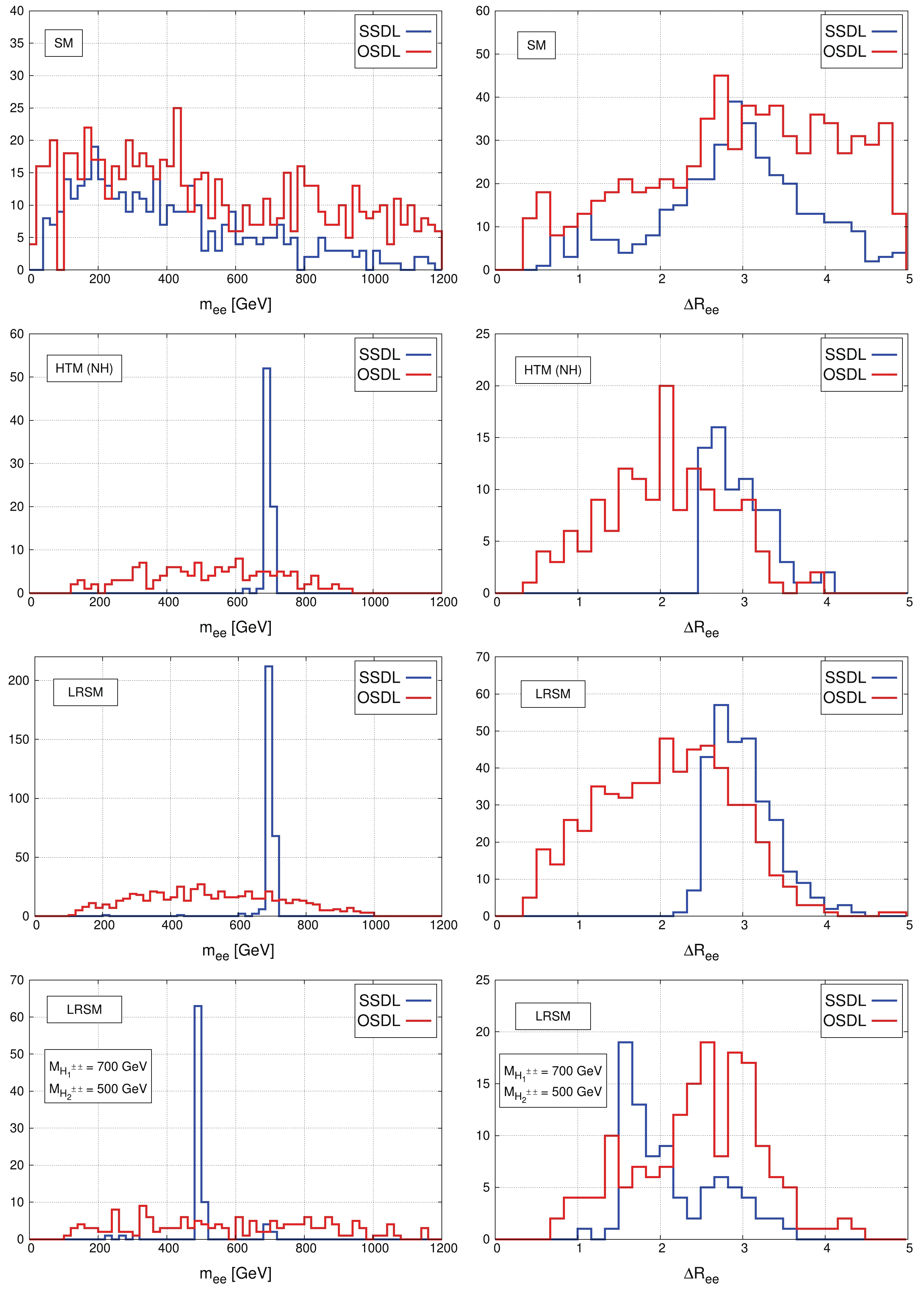
Figure 14. (color online) Dilepton distributions for
$e^+e^- \to 4e$ . In the left column,$m_{ee}$ distributions are shown for the SM background (top figure); the$ {\texttt{HTM}}$ model with the NH scenario and benchmark parameters as given in Table 15 (second figure); the${\texttt{MLRSM}}$ with benchmark parameters for$v_R=6$ TeV as given in Table 15 (third figure). The bottom, last row plots are for the${\texttt{MLRSM}}$ with$m_{{H_1^{\pm \pm}}}=700$ GeV and$m_{{H_2^{\pm \pm}}}=500$ GeV. On the right, analogous figures for the$e-e$ separation observable$\Delta R_{ee}$ are given. -
The doubly charged Higgs boson
$ H^{\pm\pm} $ pair production at$ e^+e^- $ and pp colliders, with their subsequent decays to four charged leptons, can provide a very clear signal when searching for non-standard scalar particle effects without missing energy. We discuss a relation between the vacuum expectation value of the triplet$ v_{\Delta} $ and$ H^{\pm\pm} $ couplings with leptons, taking into account constraints on$ v_{\Delta} $ coming from low energy studies connected with the ρ-parameter, muon$ (g-2)_{\mu} $ , lepton flavor violation,$ e^+e^- $ , LHC processes, and neutrino oscillations (normal and inverse mass scenarios). The low energy experiments rule out$ v_{\Delta} $ below 10 eV (for$ M_{H^{\pm\pm}} \sim 700 $ GeV) for both normal and inverted hierarchies, and the strongest limit for non-zero mass of the lightest neutrino comes from LFV$ \mu \to 3e $ ; see Fig. 5 and Table 5. As the Yukawa$ H^{\pm \pm}-l-l' $ couplings are inversely proportional to$ v_{\Delta} $ , the t-channel$e^+ e^- \to H^{++} H^{--}$ process could be enhanced; however, neutrino oscillation data make it very small, and the s-channel dominates over the allowed$ v_{\Delta} $ ; see Fig. 7. Similarly, Yukawa$ H^{\pm \pm}_{1,2}-l-l' $ couplings in the$ {\texttt{MLRSM}}$ could dominate the cross section for$e^+ e^- \to H^{++}_{1,2} H^{--}_{1,2}$ ; however,$ e^+e^- $ Bhabha and Møller processes make it below the s-channel contribution; see Fig. 8. These two cases show nicely how important the present SM and LFV experimental data are, allowing the proper prediction of BSM signals in collider studies. Taken together,$ H^{\pm\pm} $ pair production processes in the$ {\texttt{HTM}}$ and$ {\texttt{MLRSM}}$ are comparable, although larger in the$ {\texttt{MLRSM}}$ . The contributions of individual$ H_{1}^{\pm \pm} $ and$ H_{2}^{\pm \pm} $ pair production channels in the$ {\texttt{MLRSM}}$ and$ H^{\pm \pm} $ in the$ {\texttt{HTM}}$ are discussed. The contributions change with HL-LHC and FCC-ee/CEPC center of mass energies. QCD NLO k-factors are discussed and taken into account in the$ H^{\pm \pm} $ pair production and four lepton processes. Taking into account the present bounds on the$ {\texttt{MLRSM}}$ parameters, additional contributions from both the right-handed current and extra scalar particles within the$ {\texttt{MLRSM}}$ do not make much difference.Still, assuming non-universality of leptonic decays, and as a result of the field richness of the
$ {\texttt{MLRSM}}$ , branching ratios for the$ H^{\pm \pm} $ decays can be very different in both models, leading to different final signals.We discuss the same
$ H^{\pm\pm} $ masses in both models. Taking into account all leptonic decays, we show that the LHC experimental data still allow for an$ H^{\pm\pm} $ mass as small as 700 GeV. We take this as the first scenario; the second is for a$ H^{\pm\pm} $ mass equal to 1 TeV.We carefully discuss possible decay channels and finally make predictions for the complete process
$ pp \to H^{++} H^{–} \to 4l $ . In both models, we optimized parameters to separately maximize$ e^+e^-(pp) \to 4e $ and$ e^+e^- (pp) \to 4 \mu $ signals, at the same time remaining in agreement with all experimental constraints coming from other considered processes.The results are given in Table 15 and Table 16. There are many interesting conclusions that can be drawn from them, as discussed in Section V.E. In general, because of kinematic cuts and the chosen parameters,
$ 4\mu $ signals dominate over$ 4e $ signals. The latter signals are in most cases at best at the level of the SM background, both for lepton and hadron colliders. This situation provides a method to discriminate between the two models. In fact, the most interesting situation, in which the$ v_R $ in the$ {\texttt{MLRSM}}$ is relatively large, above the sensitivity of the LHC (we took$ v_R = 15 $ TeV), does not provide constraints on the model parameters that are too strict, and the discovery signals can be large for$ e^+e^- (pp) \to 4 \mu $ . In particular, for the HL-LHC and FCC-hh cases, detectable signals that would exceed the SM background are possible only for the$ {\texttt{MLRSM}}$ . This conclusion is rather stable over changes of model parameters, for the considered kinematic cuts. Although analysis of dilepton distributions can further assist detection of small BSM signals that are comparable to or below the SM background, they show similar patterns for both models and do not help to discriminate between the$ {\texttt{HTM}}$ and$ {\texttt{MLRSM}}$ .With the most straightforward setups, relying only on the production and decay total counting of events, we can discriminate models and show the channels in which we should look. We think that our work is an exemplary case study, and from the minimal considerations, more sophisticated approaches can follow. As an outlook for further studies, a discussion of
$ e^\pm e^\pm \mu^\mp \mu^\mp $ and$ e^\pm e^\mp \mu^\pm \mu^\mp $ channels might also be appropriate, as well as four-lepton signal analysis with final state polarization. It will be also interesting to investigate, for chosen benchmark points, processes with single produced$ H^{\pm \pm} $ or single charged Higgs scalars and the associated gauge bosons. For such cases, the SM background will be much larger, but this does not exclude positive BSM signals. -
We thank Joydeep Chakrabortty for useful discussions and Dipankar Das for his help with the FeynRules model.
-
The Higgs Triplet Model extends the Higgs sector of the SM by adding one scalar
$ SU(2)_L $ triplet ($ \Delta $ ) with hypercharge$ Y = 2 $ to the SM doublet Φ (following the convention$ Q = \dfrac{1}{2}Y+T_3 $ ).The most general scalar potential is given by [41]
$\tag{A1} \begin{aligned}[b] V =& -m_{\Phi}^2\left(\Phi^{\dagger}\Phi\right) + \frac{\lambda}{4}\left(\Phi^{\dagger}\Phi\right)^2 + M_{\Delta}^2{\rm{Tr}}\left(\Delta^{\dagger}\Delta\right)\\ & +\left[\mu \left(\Phi^Ti\sigma_2\Delta^{\dagger}\Phi\right) + {\rm{h.c.}} \right] \\ & +\lambda_1\left(\Phi^{\dagger}\Phi\right){\rm{Tr}}\left(\Delta^{\dagger}\Delta\right) +\lambda_2\left[{\rm{Tr}}\left(\Delta^{\dagger}\Delta\right)\right]^2\\& +\lambda_3{\rm{Tr}}\left[\left(\Delta^{\dagger}\Delta\right)^2\right] +\lambda_4 \Phi^{\dagger}\Delta \Delta^{\dagger}\Phi \,. \end{aligned} $

Without loss of generality, we can take all the parameters to be real [31, 186]. Denoting by
$ v_{\Delta} $ and$ v_\Phi $ the vacuum expectation values (VEV's) of the doublet and triplet$\tag{A2} m_{\Phi}^2 = \frac{\lambda}{4} v_\Phi^2 +\frac{(\lambda_1+\lambda_4)}{2} v_{\Delta}^2 -\sqrt{2}\mu \: v_{\Delta} \,, $

$\tag{A3} M_{\Delta}^2 = -(\lambda_2+\lambda_3) \: v_{\Delta}^2 - \frac{(\lambda_1+\lambda_4)}{2} v_\Phi^2 +\frac{\mu}{\sqrt{2}} \frac{v_\Phi^2}{v_{\Delta}} \,. $

We represent the scalar multiplets in the following way
$\tag{A4} \begin{aligned}[b]&\Phi = \frac{1}{{\sqrt 2 }}\left( {\begin{array}{*{20}{c}} {\sqrt 2 w_\Phi ^ + }\\ {{v_\Phi } + {h_\Phi } + {\rm i}{z_\Phi }} \end{array}} \right){\mkern 1mu} ,\\&\Delta = \frac{1}{{\sqrt 2 }}\left( {\begin{array}{*{20}{c}} {w_\Delta ^ + }&{\sqrt 2 {\delta ^{ + + }}}\\ {{v_\Delta } + {h_\Delta } + {\rm i}{z_\Delta }}&{ - w_\Delta ^ + } \end{array}} \right){\mkern 1mu} . \end{aligned}$

The triplet VEV
$ v_{\Delta} $ is expected to be at most on the order$ {{\cal{O}} \left(1 \right)}\; {\rm{GeV}} $ to keep the electroweak ρ-parameter$ \sim $ 1 [41, 42, 44, 175, 187] (see Section III.B for more details). The electroweak VEV is then given by$\tag{A5} v = \sqrt{v_\Phi^2+2v_{\Delta}^2} \simeq 246\; {\rm{GeV}} \, . $

The Yukawa sector contains the complete SM Yukawa Lagrangian, along with an extra part for the triplet
$\tag{A6} {\cal{L}}_Y^{\Delta} = \frac{1}{2}{\cal{Y}}_{\ell\ell'} L_\ell^T C^{-1} {\rm i}\sigma_2 \Delta L_{\ell'} + {\rm{h.c.}} \,, $

where C is the charged conjugation operator,
$ {\cal{Y}}_{\ell\ell'} $ is the symmetric Yukawa matrix, and$\tag{A7} {L_\ell } = {\left( {\begin{array}{*{20}{c}} {{\nu _\ell }}\\ \ell \end{array}} \right)_L}{\mkern 1mu} ,\;\;\;\left[ {\ell = e,\mu ,\tau } \right] , $

are the left handed
$ SU(2) $ doublets for the three lepton generations. After spontaneous symmetry breaking (SSB), the Yukawa couplings in Eq. (A6) will lead to the Majorana mass matrix for the left handed neutrinos. The same term in the Lagrangian is responsible for the interaction between doubly charged scalar particles and charged leptons. The$ H^{\pm\pm}-l^{\mp}-l'^{\mp} $ vertex breaks the lepton number (see Sections II and III). The fields,$ \delta^{\pm\pm} = $ $ H^{\pm\pm} $ , represent the doubly charged scalar with the mass$\tag{A8} M_{H^{\pm\pm}}^2 = \frac{\mu v_\Phi^2}{\sqrt{2}v_{\Delta}} -\frac{\lambda_4}{2}v_\Phi^2 -\lambda_3 v_{\Delta}^2 \,. $

To obtain physical states for neutral and singly charged particles, appropriate rotation of fields in the CP-odd and CP-even sectors must follow
$\tag{A9} \begin{pmatrix} G_0 \\ A \end{pmatrix} = \begin{pmatrix} \cos\beta' & \sin\beta' \\ -\sin\beta' & \cos\beta' \end{pmatrix} \begin{pmatrix} z_\Phi \\ z_{\Delta} \end{pmatrix} \,, \; \; \; {\rm{with}} \; \; \tan\beta' = \frac{2v_{\Delta}}{v_\Phi} \,, $

$\tag{A10}\begin{aligned}[b]& \left( {\begin{array}{*{20}{c}} h\\ H \end{array}} \right) = \left( {\begin{array}{*{20}{c}} {\cos \alpha }&{\sin \alpha }\\ { - \sin \alpha }&{\cos \alpha } \end{array}} \right)\left( {\begin{array}{*{20}{c}} {{h_\Phi }}\\ {{h_\Delta }} \end{array}} \right){\mkern 1mu} ,\\\;\;{\rm{with}}&\;\tan 2\alpha = \frac{{\sqrt 2 \mu {v_\Phi } - ({\lambda _1} + {\lambda _4}){v_\Delta }{v_\Phi }}}{{\dfrac{{\mu v_\Phi ^2}}{{2\sqrt 2 {v_\Delta }}} + ({\lambda _2} + {\lambda _3})v_\Delta ^2 - \dfrac{{\lambda v_\Phi ^2}}{4}}}{\mkern 1mu} .\end{aligned} $

Furthermore, we use an approximation
$ \sin{\alpha}\; \sim\; $ $ 2\dfrac{v_{\Delta}}{v_\Phi}\; \rightarrow\; 0 $ [85]; hence, the neutral scalar masses become$\tag{A11} M_A^2 = \frac{\mu}{\sqrt{2}v_{\Delta}}(v_\Phi^2+4v_{\Delta}^2), $

$\tag{A12}\begin{aligned}[b] M_h^2 =& \lambda v_\Phi^2 \cos^2\!\alpha + \left(\frac{\mu v_\Phi^2}{\sqrt{2}v_{\Delta}} + 2 v_{\Delta}^2 (\lambda_2+\lambda_3) \right) \sin^2\!\alpha \\&+ 2 \left( v_\Phi v_{\Delta} (\lambda_1+\lambda_4) - \sqrt{2}\mu v_\Phi \right) \cos{\alpha}\sin{\alpha},\end{aligned}$

$\tag{A13}\begin{aligned}[b] M_{H}^2 =& \lambda v_\Phi^2 \sin^2\!\alpha + \left(\frac{\mu v_\Phi^2}{\sqrt{2}v_{\Delta}} + 2 v_{\Delta}^2 (\lambda_2+\lambda_3) \right) \cos^2\!\alpha \\&- 2 \left( v_\Phi v_{\Delta} (\lambda_1+\lambda_4) - \sqrt{2}\mu v_\Phi \right) \cos{\alpha}\sin{\alpha}.\end{aligned} $

In the singly charged sector rotation of fields and masses are the following
$\tag{A14} \begin{pmatrix} G^\pm \\ H^\pm \end{pmatrix} = \begin{pmatrix} \cos\beta & \sin\beta \\ -\sin\beta & \cos\beta \end{pmatrix} \begin{pmatrix} w_\Phi^\pm \\ w_{\Delta}^\pm \end{pmatrix} \,, \; \; \; {\rm{with}} \; \; \tan\beta = \frac{\sqrt{2}v_{\Delta}}{v_\Phi} \,, $

to obtain the charged Goldstone (
$ G^\pm $ ) along with a singly charged scalar ($ H^\pm $ ) with mass$\tag{A15} M_{H^{\pm}}^2 = \frac{(2\sqrt{2}\mu-\lambda_4v_{\Delta})}{4v_{\Delta}}(v_\Phi^2+2v_{\Delta}^2) \,. $

The
$ H^\pm $ and$ H^{\pm\pm} $ scalar's squared masses (A15) and (A8) contain terms proportional to$ v_\Phi^2 $ and are inversely proportional to the triplet VEV$ v_{\Delta} $ , which should be less than$ {\cal{O}}(1\; {\rm{GeV}}) $ (see Section III.B). This means that$ M_{H^\pm} $ and$ M_{H^{\pm\pm}} $ can be at the level of a few hundred GeV or higher. The latest LHC bounds on the doubly charged scalar masses vary from 450 to 870 GeV, depending on the decay modes, assuming that$ {\rm{BR}}\left(H^{\pm\pm} \to l^\pm l^\pm \right) \geqslant 10 $ % [55]. Photon-photon fusion studies [188] set a bound on$ M_{H^{\pm\pm}} $ at the level of 748 GeV. Limits coming from$ e^+ e^- $ colliders are significantly lower; from the L3 Collaboration (LEP), the limit is approximately 100 GeV [101]. This bound comes with the assumption that the t-channel is negligible (Fig. 1) as suppressed by the low$ H^{\pm\pm}-l-l $ coupling. For singly charged scalar masses, the mass bound is even lower, i.e.,$ M_{H^\pm} $ = 80 GeV [123].In this paper, we assume that the neutral and charged scalar masses are degenerate ③, which means that
$ M_{H^{\pm\pm}} = M_{H^\pm} = M_{H} = M_A $ . This choice protects the proper ranges of the T-parameter and potential unitarity for$ v_{\Delta} \lesssim 1 $ GeV [85, 86]. -
The SSB occurs in two steps:
$ SU(2)_R \otimes $ $ U(1)_{B-L} \to $ $ U(1)_Y $ , and$ SU(2)_L \otimes U(1)_Y \to $ $ U(1)_{em} $ . To achieve this symmetry breaking, we choose a traditional spectrum of Higgs sector multiplets with a bidoublet and two triplets [29, 38, 39, 87, 189].$\tag{A16} \phi = \left( {\begin{array}{*{20}{l}} {\phi _1^0\;}&{\;\phi _1^ + }\\ {\phi _2^ - }&{\phi _2^0} \end{array}} \right) \equiv [2,2,0], $

$\tag{A17} {\Delta _{L(R)}} = \left( {\begin{array}{*{20}{c}} {\delta _{L(R)}^ + /\sqrt 2 }&{\delta _{L(R)}^{ + + }}\\ {\delta _{L(R)}^0}&{ - \delta _{L(R)}^ + /\sqrt 2 } \end{array}} \right) \equiv [3(1),1(3),2], $

where the quantum numbers in square brackets are given for
$ SU(2)_L $ ,$ SU(2)_R $ , and$ U(1)_{B-L} $ groups, respectively.The VEVs of the scalar fields can be recast in the following form:
$\tag{A18}\left\langle \phi \right\rangle {\rm{ }} = \left( {\begin{array}{*{20}{c}} {{\kappa _1}/\sqrt 2 }&0\\ {0\;}&{{\kappa _2}/\sqrt 2 } \end{array}} \right),{\rm{ }}\left\langle {{\Delta _{L,R}}} \right\rangle = \left( {\begin{array}{*{20}{c}} 0&0\\ {{v_{L,R}}/\sqrt 2 \;}&0 \end{array}} \right).$

The VEVs of the right-handed triplet (
$ \Delta_R $ ) and the bi-doublet ($ \phi $ ) propel the respective symmetry breaking:$ SU(2)_R \otimes U(1)_{B-L}\to U(1)_Y $ and$SU(2)_L \otimes U(1)_Y \to $ $ U(1)_{em}$ . As$ v_L\ll \kappa_{1,2}\ll v_R $ , we can safely take$ v_L = 0 $ .The full scalar potential includes left and right-handed triplets [29, 38, 39]:
$ \begin{aligned}[b] V(\phi,\Delta_L,\Delta_R)\! =\!& + \lambda_1\bigg\{\Big({\rm{Tr}}\big[\phi^{\dagger} \phi\big]\Big)^2\bigg\} + \lambda_2\bigg\{ \Big({\rm{Tr}}\big[\tilde{\phi}\phi^{\dagger}\big]\Big)^2\\&+\Big({\rm{Tr}}\big[\tilde{\phi}^{\dagger} \phi\big]\Big)^2 \bigg\} + \lambda_3\bigg\{{\rm{Tr}}\big[\tilde{\phi}\phi^{\dagger}\big]{\rm{Tr}}\big[\tilde{\phi}^{\dagger} \phi\big] \bigg\} \\& + \lambda_4 \bigg\{ {\rm{Tr}}\big[\phi^{\dagger} \phi\big]\Big({\rm{Tr}}\big[\tilde{\phi}\phi^{\dagger}\big] +{\rm{Tr}}\big[\tilde{\phi}^{\dagger} \phi\big]\Big) \bigg\}\\ &+ \rho_1 \bigg\{ \Big({\rm{Tr}}\big[\Delta_L \Delta_L^{\dagger}\big]\Big)^2+\Big(\Delta_R \Delta_R^{\dagger}\Big)^2 \bigg\} \\ & +\! \rho_2\! \bigg\{\!{\rm{Tr}}\big[\Delta_L \Delta_L\big]{\rm{Tr}}\big[\Delta_L^{\dagger} \Delta_L^{\dagger}\big] \!\!+\!\!{\rm{Tr}}\big[\Delta_R \Delta_R\big]{\rm{Tr}}\big[\Delta_R^{\dagger} \Delta_R^{\dagger}\big] \bigg\} \end{aligned} $

$\tag{A19} \begin{aligned}[b]& + \rho_3 \bigg\{{\rm{Tr}}\big[\Delta_L\Delta_L^{\dagger}\big]\;{\rm{Tr}}\big[\Delta_R\Delta_R^{\dagger}\big]\bigg\}\\ &+ \rho_4 \bigg\{\!{\rm{Tr}}\big[\Delta_L\Delta_L \big] {\rm{Tr}}\big[\Delta_R^{\dagger} \Delta_R^{\dagger}\big] \!\!+\!\! {\rm{Tr}}\big[\Delta_L^{\dagger} \Delta_L^{\dagger} \big] {\rm{Tr}}\big[\Delta_R \Delta_R \big] \bigg\} \\& + \alpha_1 \bigg\{{\rm{Tr}}\big[\phi^{\dagger} \phi\big]\Big({\rm{Tr}}\big[\Delta_L\Delta_L^{\dagger}\big] +{\rm{Tr}}\big[\Delta_R\Delta_R^{\dagger}\big]\Big)\bigg\} \\& + \alpha_2 \bigg\{{\rm{Tr}}\big[\phi\tilde{\phi}^{\dagger}\big]{\rm{Tr}}\big[\Delta_R\Delta_R^{\dagger}\big] + {\rm{Tr}}\big[\phi^{\dagger}\tilde{\phi}\big]{\rm{Tr}}\big[\Delta_L\Delta_L^{\dagger}\big]\bigg\} \\& + \alpha_2^* \bigg\{{\rm{Tr}}\big[\phi^{\dagger}\tilde{\phi}\big]{\rm{Tr}}\big[\Delta_R\Delta_R^{\dagger}\big] + {\rm{Tr}}\big[\tilde{\phi}^{\dagger}\phi\big]{\rm{Tr}}\big[\Delta_L\Delta_L^{\dagger}\big]\bigg\} \\ &+ \alpha_3 \bigg\{ {\rm{Tr}}\big[\phi \phi^{\dagger} \Delta_L \Delta_L^{\dagger}\big] +{\rm{Tr}}\big[\phi^{\dagger} \phi \Delta_R \Delta_R^{\dagger}\big]\bigg\}\\& - \mu_1^2{\rm{Tr}}[\phi^{\dagger}\phi]-\mu_2^2({\rm{Tr}}[\widetilde{\phi}\phi^{\dagger}]+{\rm{Tr}}[\widetilde{\phi}^{\dagger}\phi])\\& - \mu_3^2({\rm{Tr}}[\Delta_L\Delta_L^{\dagger}]+{\rm{Tr}}[\Delta_R\Delta_R^{\dagger}]). \end{aligned} $

Even though in the
$ {\texttt{HTM}}$ and$ {\texttt{MLRSM}}$ we have left-handed triplets, the$ {\texttt{HTM}}$ is not a simple subset of the$ {\texttt{MLRSM}}$ , as the scalar potentials, SSB mechanism, VEVs, and underlying physics that follow are different. The scalar potential (A19) in the$ {\texttt{MLRSM}}$ is much more complicated than its counterpart in the$ {\texttt{HTM}}$ : in the$ {\texttt{MLRSM}}$ , the triplet$ \Delta_L $ is intertwined with the right-handed multiplet$ \Delta_R $ and bidoublet$ \phi $ . This makes relations among physical and unphysical Higgs boson fields rather complex in the$ {\texttt{MLRSM}}$ . Here, significant relations include those between the$ \alpha_3 $ scalar potential parameter (which includes a mixture of a bidoublet and triplet fields) and$ \rho_1,\rho_3 $ scalar potential parameters for doubly charged Higgs boson masses given in Eq. (A29) and Eq. (A30) below. In agreement with experimental constraints for singly charged and neutral scalar fields, these parameters give the lowest limits for doubly charged Higgs masses, as discussed in [166]. Moreover, because of the Yukawa couplings of left- and right-handed leptons with the bidoublet in Eq. (A39), the doubly charged Higgs bosons couple differently to leptons in each model. Consequently, both model neutrino mass relations are different; in the$ {\texttt{HTM}}$ , they are restricted directly by neutrino oscillation data, as discussed in the main text.After SSB of the potential, Eq. (A19), the mass matrix that includes
$ M_{H_0^0} $ can be written in the following form (for details, see [29])$\tag{A20} M = \left( {\begin{array}{*{20}{c}} {2{\epsilon ^2}{\lambda _1}}&{2{\epsilon ^2}{\lambda _4}}&{{\alpha _1}\epsilon }\\ {2{\epsilon ^2}{\lambda _4}}&{\dfrac{1}{2}\left[ {4(2{\lambda _2} + {\lambda _3}){\epsilon ^2} + {\alpha _3}} \right]}&{2{\alpha _2}\epsilon }\\ {{\alpha _1}\epsilon }&{2{\alpha _2}\epsilon }&{2{\rho _1}} \end{array}} \right). $

Expanding eigenvalues of this matrix for a small
$ \epsilon = \sqrt{\kappa_1^2+\kappa_2^2}/v_R $ parameter, we obtain$\tag{A21} M_{H_0^0}^2 = 2 \left( \lambda_1 - \frac{\alpha_1^2}{4\rho_1} \right)(\kappa_1^2+\kappa_2^2) \qquad \; \simeq (125 \; {\rm{GeV}})^2. $

The analytic mass formulas for other scalar bosons in the
$ {\texttt{MLRSM}}$ as a function of quartic couplings and$ v_R $ can be written as [56]$\tag{A22} M_{H_1^0}^2 = \frac{1}{2} \alpha_3 v_R^2 \qquad > (10 \; {\rm{TeV}})^2, $

$\tag{A23} M_{H_2^0}^2 = 2 \rho_1 v_R^2, $

$\tag{A24} M_{H_3^0}^2 = \frac{1}{2} (\rho_3-2\rho_1) v_R^2 \qquad > (55.4 \; {\rm{GeV}})^2, $

$\tag{A25} M_{A_1^0}^2 = \frac{1}{2} \alpha_3 v_R^2 - 2(\kappa_1^2+\kappa_2^2) (2\lambda_2-\lambda_3)\;\; > (10 \; {\rm{TeV}})^2, $

$\tag{A26} M_{A_2^0}^2 = \frac{1}{2} (\rho_3 - 2 \rho_1) v_R^2 $

$\tag{A27} M_{H_1^\pm}^2 = \frac{1}{2} (\rho_3 - 2 \rho_1) v_R^2 + \frac{1}{4}\alpha_3 (\kappa_1^2+\kappa_2^2), $

$\tag{A28} M_{H_2^\pm}^2 = \frac{1}{2} \alpha_3 v_R^2 + \frac{1}{4} \alpha_3 (\kappa_1^2+\kappa_2^2) \qquad > (10 \; {\rm{TeV}})^2, $

$\tag{A29} M_{H_1^{\pm\pm}}^2 = \frac{1}{2} (\rho_3-2\rho_1) v_R^2 +\frac{1}{2}\alpha_3 (\kappa_1^2+\kappa_2^2), $

$\tag{A30} M_{H_2^{\pm\pm}}^2 = 2 \rho_2 v_R^2 + \frac{1}{2}\alpha_3 (\kappa_1^2+\kappa_2^2), $

where
$ \kappa_1,\kappa_2 $ are VEVs of the bidoublet, and$ \sqrt{\kappa_1^2+\kappa_2^2} $ must be equal to the electroweak symmetry breaking scale v; see (A5). We assume that$ \kappa_1 = v = 246 $ GeV and$ \kappa_2 \to 0 $ . Some explicit masses of Higgs bosons relevant for$ H^{\pm \pm} $ BRs in Section V.C come from restrictions discussed in [56].In the
$ {\texttt{MLRSM}}$ , relations among physical and unphysical fields (“G” stands for Goldstone modes) are$\tag{A31} \phi_1^0 \simeq \frac{1}{\sqrt{2}}\left[ H_0^0+{\rm i} \tilde{ G_1^0} \right] , $

$\tag{A32} \phi_2^0 \simeq \frac{1}{\sqrt{2}}\left[ H_1^0-{\rm i} A_1^0 \right], $

$\tag{A33} \delta_R^0 = \frac{1}{\sqrt{2}}\left( H_2^0+{\rm i}G_2^0 \right),\;\; \delta_L^0 = \frac{1}{\sqrt{2}} \left( H_3^0+{\rm i}A_2^0 \right), $

$\tag{A34} \delta_L^+ = H_1^+,\;\;\;\delta_R^+ \simeq G_R^+ , $

$\tag{A35} \phi_{1}^+ \simeq H_2^+, \;\;\; \phi_{2}^+ \simeq G_L^+, $

$\tag{A36} \delta_R^{\pm \pm} = H_1^{\pm \pm},\;\;\; \delta_L^{\pm \pm} = H_2^{\pm \pm}. $

The structure of the Higgs potential in a general framework of left-right symmetric models has been discussed in detail in [29, 38]. We adopt this in our studies. In particular, to retain the invariant Majorana Yukawa couplings of the leptons to the Higgs triplet, the potential does not include terms with all multiplets (bidoublet, two triplets) present simultaneously, e.g.,
${\rm Tr}[\phi \Delta_R\phi^{\dagger} \Delta_L^{\dagger}]\;+{\rm h.c.}$ (in [29, 38], denoted as$ \beta_i $ -type terms). In the limit of vanishing$ \beta_i $ terms, the doubly charged Higgs scalar$ 2 \times 2 $ mass matrix is diagonal and does not include the mixed mass terms$ \delta_L^{\pm \pm}\delta_R^{\mp \mp} $ . These restrictions simplify the form of doubly charged mass terms, as given in the manuscript and Eqs. (A29) and (A30). This means that in the$ {\texttt{MLRSM}}$ (and other extensions when gauge couplings$ g_L \neq g_R $ ), doubly charged Higgs triplets in$ \Delta_{L,R} $ are physical fields. There is no mixing angle between two doubly charged Higgs bosons in the$ {\texttt{MLRSM}}$ , and the mass matrix that appears there for unphysical fields is diagonal from the very beginning. This no-mixing feature is also true in general where the$ \beta_i $ -type terms are allowed, in the limit$ v_R \gg \kappa_{1,2} $ . -
In the
$ {\texttt{MLRSM}}$ , because of the additional heavy states, the neutrino sector and Yukawa couplings are more complicated than in the$ {\texttt{HTM}}$ . Here, we argue that because of an energy scale difference between$ v_R $ and the low-energy bidoublet VEV$ \kappa \equiv \sqrt{\kappa_1^2+\kappa_2^2} $ ,$ \kappa \ll v_R $ , the see-saw mechanism is possible and low energy LFV signals are suppressed because of the high$ v_R $ and heavy neutrino masses. To see this, the most general doubly charged couplings to leptons, which take into account mixing matrices, read [39]$\tag{A37} \begin{aligned}[b] \delta_R^{++}\bar{l}_L^{\prime c}h_Ml^\prime_R\! +\!{\rm h.c.} \!=\!& \frac{1}{\sqrt{2}v_R}\!\sum\limits_{l,k} \!\left\{ \delta_R^{++} \left[ l^T_{l}C \left( K^T_R \left( M_\nu \right)_{\rm diag} K_R \right)_{lk} P_R l_{k} \right] \right. \\&+ \left. \delta_R^{–} \left[ \bar{l}_{l} \left( K^{\dagger}_R \left( M_\nu \right)_{\rm diag} K_R^\ast \right)_{lk} P_L C\bar{l}^T_{k} \right] \right\}, \end{aligned} $

$\tag{A38} \begin{aligned}[b] \delta_L^{++}\bar{l}_R^{\prime c}h_Ml^\prime_L +{\rm h.c.} =& \frac{1}{\sqrt{2}v_R}\sum\limits_{l,k} \left\{ \delta_L^{++} \left[ l^T_{k}C \left( K_L^T X K_L^\ast \right)_{kl} P_L l_{l} \right] \right. \\&+ \left. \delta_L^{–} \left[ \bar{l}_{k} \left( K_L^T X^\ast K_L^\ast \right)_{kl} P_R C\bar{l}^T_{l} \right] \right\}, \end{aligned} $

where
$X = (K_L^\ast K_R^T) \left( M_\nu \right)_{\rm diag} (K_R K_L^{\dagger})$ .These couplings originate from the Yukawa part of the Lagrangian for additional scalar triplets and a bidoublet
$ \phi $ :$\tag{A39} - \bar{L}_L \left[ h_l \phi +\tilde{h}_l \tilde{\phi} \right] L_R - {\rm i}\bar{L}_R^c \sigma_2 \Delta_L h_M L_L -{\rm i}\bar{L}_L^c \sigma_2 \Delta_R h_M L_R + {\rm h.c.} $

The uniqueness of left- and right-handed couplings for positively and negatively charged doubly charged Higgs bosons to leptons in Eq. (A37) and Eq. (A38) is due to the Feynman rules and flow of the charged currents in vertices, as explained at length in [190]. The relations between physical and unphysical scalar, gauge, and fermion fields are embedded in our FeynRules package to calculate BRs and cross sections. We also mentioned that for neutral scalars, because of the bidoublet coupling in Eq. (A39) to both left- and right-handed leptons, there is a mixture of scalar fields coming from left and right triplets; however, as given in Eqs. (A31)-(A36), for
$ v_R \gg \kappa_{1,2} $ , most of the mixings are negligible.Diagonalization of the resulting neutrino mass matrix
$\tag{A40}\begin{aligned}[b] {M_\nu } =& \left( {\begin{array}{*{20}{c}} 0&{{M_D}}\\ {M_D^T}&{{M_R}} \end{array}} \right),\\ {M_R} =&\sqrt 2 {h_M}{v_R}, \end{aligned}$

proceeds with the help of a unitary 6
$ \times $ 6 matrix U$\begin{aligned}[b] {U^T}{M_\nu }U =& {({M_\nu })_{\rm diag}},\\ U = &\left( {\begin{array}{*{20}{c}} {K_L^*}\\ {{K_R}} \end{array}} \right). \end{aligned}$

This procedure leads to the introduction of the
$ K_L $ and$ K_R $ submatrices in Eq. (A37) and Eq. (A38) [143, 191].The charged lepton mass matrix is diagonalized by
$ {V^l_{L,R}}_{3\times 3} $ $ {V^l_L}^{\dagger} M_l V^l_R = (M_l)_{\rm diag}. $

In addition to charged lepton and neutrino mass terms, Lagrangian Eq. (A39) contains scalar-lepton interactions.
$\left( M_\nu \right)_{\rm diag}$ contains three light neutrinos, and their contribution to couplings Eq. (A38) and Eq. (A37) are negligible. To see the amount of the heavy neutrino contributions to Eq. (A38) and Eq. (A37), we note that the structure of the$ K_L $ and$ K_R $ mixing matrices are as follows [143, 191]:$\tag{A41}{({K_L})_{{l_i}{\nu _j}}} = \left( {\begin{array}{*{20}{c}} {e\;\;\mu \;\;\tau \;\;\;\;\;\;\;\;\;\;\;\;\;\;\;\;\;\;\;\;\;\;\;\;\;\;}\\ {\left. {\left( {\begin{array}{*{20}{c}} \cdot & \cdot & \cdot \\ \cdot & \cdot & \cdot \\ \cdot & \cdot & \cdot \end{array}} \right)} \right\}{\rm{light}}\;\;{\rm{neutrinos}}}\\ {\left. {\left( {\begin{array}{*{20}{c}} \cdot & \cdot & \cdot \\ \cdot & \cdot & \cdot \\ \cdot & \cdot & \cdot \end{array}} \right)} \right\}{\rm{heavy}}\;\;{\rm{neutrinos}}} \end{array}} \right)\;\sim \left( {\begin{array}{*{20}{c}} {}\\ {{\cal{O}}(1)}\\ {}\\ {}\\ {{\cal{O}}\left( {\dfrac{1}{{{m_N}}}} \right)}\\ {} \end{array}} \right), $

$\tag{A42} {({K_R})_{{l_i}{\nu _j}}} = \left( {\begin{array}{*{20}{c}} {e\;\;\mu \;\;\tau \;\;\;\;\;\;\;\;\;\;\;\;\;\;\;\;\;\;\;\;\;\;\;\;\;\;}\\ {\left. {\left( {\begin{array}{*{20}{c}} \cdot & \cdot & \cdot \\ \cdot & \cdot & \cdot \\ \cdot & \cdot & \cdot \end{array}} \right)} \right\}{\rm{light}}\;\;{\rm{neutrinos}}}\\ {\left. {\left( {\begin{array}{*{20}{c}} \cdot & \cdot & \cdot \\ \cdot & \cdot & \cdot \\ \cdot & \cdot & \cdot \end{array}} \right)} \right\}{\rm{heavy}}\;\;{\rm{neutrinos}}} \end{array}} \right)\;\sim \left( {\begin{array}{*{20}{c}} {}\\ {{\cal{O}}\left( {\dfrac{1}{{{m_N}}}} \right)}\\ {}\\ {}\\ {{\cal{O}}(1)}\\ {} \end{array}} \right). $

Off-diagonal elements for heavy neutrino couplings in
$ K_R $ are typically also on the order of the inverse heavy neutrino mass scale; that is why the LFV couplings of leptons with doubly charged Higgs bosons are strongly suppressed, and$ \delta_{L,R}-l-l $ off-diagonal lepton couplings are suppressed by$ 1/m_N^2 $ when compared with diagonal cases.For reasons discussed in [147] and more extensively in [192], we utilize seesaw diagonal light-heavy neutrino mixings. This means that
$ W_1 $ couples primarily to light neutrinos, while$ W_2 $ couples to the heavy ones.To summarize, unlike in the HTM case, the
$ H^{\pm \pm}-l^\mp-l^\mp $ vertex does not depend on the light neutrino mixing. With$ v_L = 0 $ , the$ {\texttt{MLRSM}}$ realizes the seesaw type-I mechanism, and the light neutrino mass is due to the existence of additional heavy neutrino states and the$ v_R $ scale.We should note that it is not natural and very difficult to create non-decoupling mixings for non-diagonal
$ K_L $ and$ K_R $ matrix elements, even when some symmetries are considered in type-I seesaw models [192]. -
The diagrams in Fig. 4 present the contributions from the singly and doubly charged scalar particles to lepton flavor violating processes and to the muon
$ (g-2)_{\mu} $ . Those diagrams contain vertices$ H^{\pm\pm}-l_i-l_j $ and$ H^\pm-l_i-\nu_j $ , which originate from the Yukawa part of the Lagrangian, combining the SM Yukawa term with the triplet part, Eq. (A6)$\tag{A43} {\cal{L}}_Y = {\cal{L}}_Y^\Phi+{\cal{L}}_Y^{\Delta} = -\: {y}_{ij} \: \overline{L^i_L} \: \Phi \: {l^j}_R \; + {\cal{Y}}_{ij} \: \overline{{L^i_L}^c} \: {\rm i}\sigma_2 \: \Delta \: L^j_L \; + \; {\rm{h.c.}} $

From Eq. (A43), we obtain the interaction between charged leptons and a doubly charged scalar and the interaction of a singly charged scalar with a charged lepton and neutrino. Taking into account Eq. (A14) and Eq. (A5) and keeping in mind that
$ y_{ij} \propto \dfrac{1}{v_\Phi} $ is a SM diagonal matrix,$\tag{A44} {\cal{V}}^{\pm\pm} = \left\{ \begin{array}{l} l_i^+ - l_j^+ - H^{–} = {\rm i} \: \left( {\cal{Y}}_{ij} + {\cal{Y}}_{ji} \right) \\ l_i^- - l_j^- - H^{++} = {\rm i} \: \left( {\cal{Y}}_{ij}^* + {\cal{Y}}_{ji}^* \right) \end{array} \right., $

$\tag{A45} \begin{aligned}[b] {\cal{V}}_\Delta^\pm = \left\{ \begin{array}{c} \!\! \tilde{\nu}_i - l_j^+ - H^- = \dfrac{{\rm i}}{\sqrt{2}} \: \cos{\beta} \: \left( {\cal{Y}}_{ij} + {\cal{Y}}_{ji} \right) \\ \!\! \nu_i - l_j^- - H^+ = \dfrac{{\rm i}}{\sqrt{2}} \: \cos{\beta} \: \left( {\cal{Y}}_{ij}^* + {\cal{Y}}_{ji}^* \right) \\ \end{array} \propto \frac{\sqrt{v_\Phi^2-2v_\Delta^2}}{v_\Phi\cdot v_\Delta} \right., \end{aligned}$

$\tag{A46} {\cal{V}}_\Phi^\pm = \left\{ \begin{array}{c} \tilde{\nu_i} - l_i^- - H^+ = {\rm i} \: \sin{\beta} \: y_{i} \\ \nu_i - l_i^+ - H^- = {\rm i} \: \sin{\beta} \: y_{i} \end{array} \propto \frac{\sqrt{2} v_\Delta}{v_\Phi\sqrt{v_\Phi^2-2 v_\Delta^2}} \right. . $

Vertices
$ {\cal{V}}_\Delta^\pm $ and$ {\cal{V}}_\Delta^{\pm\pm} $ come from the same part of the Lagrangian and break the lepton flavor. Vertex$ {\cal{V}}_\Phi^\pm $ is proportional to$ v_\Delta $ , while vertex$ {\cal{V}}_\Delta^\pm $ is inversely proportional to the triplet VEV and dominates up to$ v_\Delta \sim 10^6 $ eV. Because we are interested in the lower regions of$ v_\Delta $ values, this effect is negligible. Therefore, with a good approximation for low values of$ v_\Delta $ $\tag{A47} {\cal{V}}_\Delta^\pm \equiv {\cal{V}}^\pm \simeq \frac{1}{\sqrt{2}} {\cal{V}}^{\pm\pm}. $

As discussed in Section III, the BRs of the radiative and μ-to-e conversions depend on the one-loop form factors. From Eq. (9), we can express them explicitly
$\tag{A48} \begin{aligned}[b] A_L(q^2) =& -\frac{({\cal{Y}}^*)_{ei} ({\cal{Y}})_{\mu i} }{24\sqrt{2} G_F \pi^2 }\Bigg(\frac{1}{12 M_{H^{\pm}}^2 }+\frac{f(r,s_i)}{M_{H^{\pm\pm}}^2}\Bigg), \\ A_R =& -\frac{({\cal{Y}}^* {\cal{Y}})_{e\mu }}{192\sqrt{2} G_F\pi^2 }\Bigg(\frac{1}{8 M_{H^{\pm}}^2}+\frac{1}{M_{H^{\pm\pm}}^2}\Bigg), \end{aligned} $

where
$ f(r,s_i) $ is given by$\tag{A49}\begin{aligned}[b] f(r,s_i) = &\frac{4 s_i}{r}+\log(s_i)+\Big(1-\frac{2 s_i}{r}\Big) \sqrt{1+\frac{4s_i}{r}}\\&\times\log \Bigg(\frac{\sqrt{r}+\sqrt{r+4s_i}}{\sqrt{r}-\sqrt{r+4s_i}}\Bigg), \end{aligned}$

$\tag{A50} r = \frac{-q^2}{m_{H^{\pm\pm}}^2} {,} \quad s_i = \frac{m_i^2}{m_{H^{\pm\pm}}^2}. $

We have consulted previous reports, where the analytic forms for the CLFV processes are given as follows [33, 91, 92, 104, 193]:
Radiative lepton decay
$ {{{l}}_{{i}} \to {{l}}_{{j}} {{\gamma}}} $ :The branching ratios of radiative decay processes can be given by
$ {\rm{BR}}(l_i\rightarrow l_j \gamma) = 384 \pi^2 (4\pi \alpha_{em})|A_R|^2\; {\rm{BR}}(l_i\rightarrow l_j\nu_{l_i} \overline{\nu}_{l_j}). $

Therefore, the BRs for various radiative decays can be written as
$ \begin{array}{*{20}{c}} {\begin{array}{*{20}{c}} {{\rm{BR}}(\mu \to e\gamma ) = \dfrac{{{\alpha _{em}}}}{{192\pi }}\dfrac{{|{{({Y^{\dagger} }Y)}_{e\mu }}{|^2}}}{{G_F^2}}{{\left(\dfrac{1}{{M_{{H^ \pm }}^2}} + \dfrac{8}{{M_{{H^{ \pm \pm }}}^2}}\right)}^2}\;{\rm{BR}}(\mu \to e{{\bar \nu }_e}{\nu _{\mu} }),}\\ {{\rm{BR}}(\tau \to e\gamma ) = \dfrac{{{\alpha _{em}}}}{{192\pi }}\dfrac{{|{{({Y^{\dagger} }Y)}_{e\tau }}{|^2}}}{{G_F^2}}{{\left(\dfrac{1}{{M_{{H^ \pm }}^2}} + \dfrac{8}{{M_{{H^{ \pm \pm }}}^2}}\right)}^2}\;{\rm{BR}}(\tau \to e{{\bar \nu }_e}{\nu _\tau }),}\\ {{\rm{BR}}(\tau \to \mu \gamma ) = \dfrac{{{\alpha _{em}}}}{{192\pi }}\dfrac{{|{{({Y^{\dagger} }Y)}_{\mu \tau }}{|^2}}}{{G_F^2}}{{\left(\dfrac{1}{{M_{{H^ \pm }}^2}} + \dfrac{8}{{M_{{H^{ \pm \pm }}}^2}}\right)}^2}\;{\rm{BR}}(\tau \to \mu {{\bar \nu }_{\mu} }{\nu _\tau }),} \end{array}\begin{array}{*{20}{c}} {{\rm{BR}}(\mu \to e{{\bar \nu }_e}{\nu _e}) = 100{\text{%}} ,}\\ {{\rm{BR}}(\tau \to e{{\bar \nu }_e}{\nu _\tau }) = 17.83{\text{%}} ,}\\ {{\rm{BR}}(\tau \to \mu {{\bar \nu }_{\mu} }{\nu _\tau }) = 17.41{\text{%}} .} \end{array}} \end{array} $ 
The contribution of
$ H^{\pm\pm} $ to the BRs is eight times larger than that by$ H^{\pm} $ because of the difference in the magnitude of couplings between$ {\cal{V}}^\pm $ and$ {\cal{V}}^{\pm\pm} $ in Eq. (A47); in addition, the amplitude is proportional to the particle charge (which gives an additional factor of 4).Three body decays
$ {{{l}} \to {{l}}_{{i}} {{l}}_{{j}} {{l}}_{{k}}} $ :$ \begin{array}{*{20}{l}} {{\rm{BR}}(\mu \to eee) = \dfrac{1}{{4G_F^2}}\dfrac{{|{{({Y^{\dagger} })}_{ee}}{{(Y)}_{\mu e}}{|^2}}}{{M_{{H^{ \pm \pm }}}^4}}\;{\rm{BR}}(\mu \to e\bar \nu \nu ),\;\;\;\;\;\;\;\;\;\;\;\;\;\;\;\;\;\;\;\;\;\;\;\;\;\;\;\;\;\;\;\;\;\;}\\ {{\rm{BR}}(\tau \to {l_i}{l_j}{l_k}) = \dfrac{S}{{4G_F^2}}\dfrac{{|{{({Y^{\dagger} })}_{\tau i}}{{(Y)}_{jk}}{|^2}}}{{M_{{H^{ \pm \pm }}}^4}}\;{\rm{BR}}(\tau \to \mu \bar \nu \nu ),\qquad \;\;\;\;\;\;\;S = \left\{ {\begin{array}{*{20}{l}} {1\;\;{\rm{if}}\;\;j = k}\\ {2\;\;{\rm{if}}\;\;j \ne k} \end{array}} \right..} \end{array}$ 
$ {{\mu}}- {\bf{to}}-{{e}} $ conversionIn the computation of the conversion rate of μ to e, both form factors contribute, and the analytic form can be written as
$\tag{A51}\begin{aligned}[b] {\rm{CR}}(\mu {\cal{N}}\rightarrow e{\cal{N}}^*) = \frac{\Gamma_{\rm conv}}{\Gamma_{\rm capt}} \cong\frac{2\alpha_{em}^5 G_F^2 m_{\mu}^5 Z_{\rm eff}^4 Z |F(q^2)|^2}{\Gamma_{\rm capt}}\Big|8A_R+\frac{2}{3}A_L\Big|^2. \end{aligned}$ 
Therefore, the μ-to-e conversion ratio in the nuclei field can be given as [92, 104]
$\tag{A52} \begin{aligned}[b] {\rm{CR}}(\mu {\cal{N}}\rightarrow e{\cal{N}}^*) =& \frac{\Gamma_{\rm conv}}{\Gamma_{\rm capt}} \cong \frac{\alpha_{em}^5}{36\pi^4} \frac{m_{\mu}^5}{\Gamma_{\rm capt}}Z_{eff}^4 Z |F(q^2 = -m_{\mu}^2)|^2\\& \times \Bigg |\frac{(M_\nu^{\dagger} M_\nu)_{e\mu}}{2v_\Delta^2} \Big[\frac{5}{24 m_{H^{\pm}}^2}+\frac{1}{m_{H^{\pm\pm}}^2}\Big]+\frac{1}{2v_\Delta^2 m_{H^{\pm\pm}}^2} \sum\limits_{l = e,\mu,\tau} (M_\nu)^{\dagger}_{el} f(r,s_i) (M_\nu)_{l\mu}\Bigg |^2, \end{aligned} $

where
${\Gamma_{\rm capt}} \quad -$ total muon capture rate (see Table 17),$\Gamma_{\rm capt} /{\rm{s} }^{-1}$ 

$\Gamma_{\rm capt}/{\rm{eV} }$ 

$Z_{\rm eff}$ 

${}^{197}_{\phantom{1}79} {\rm{Au}}$ 

$13.07\times 10^6$ 

$8.60\times 10^{-9}$ 

33.5 ${}^{48}_{22} {\rm{Ti}}$ 

$2.59\times 10^6$ 

$1.71\times 10^{-9}$ 

17.5 ${}^{27}_{13} {\rm{Al}}$ 

$0.7054\times 10^6$ 

$0.4643\times 10^{-9}$ 

11.5 Table 17. Total muon capture rate and effective charge for
${}^{197} {\rm{Au}}$ ,${}^{48} {\rm{Ti}}$ , and${}^{27} {\rm{Al}}$ [194].$Z_{\rm eff} -$ effective charge for the muon in the 1s state,Muon
$ ({g-2})_{\mu} $ For the case of doubly charged scalars, the cumulative effects of muon
$ (g-2)_{\mu} $ and lepton flavor violation have been discussed in detail in [104, 195, 196], and that for a triplet scalar has been discussed in [90].The contributions to muon
$ (g-2) $ from doubly and singly charged scalars are shown in Fig. 15. The final formulas for$ H^{\pm \pm} $ and$ H^{\pm} $ read
Figure 15. Feynman diagrams representing the contribution to
$(g-2)_\mu$ within the HTM.$\tag{A53}\begin{aligned}[b] \left[\Delta a_{\mu}\right]_{H^{\pm \pm}} =& - \sum\limits_l f^l \times\Bigg\{\frac{2 m_{\mu}^2 |{\cal{V}}_{\mu l}^{{\pm\pm}}|^2}{8\pi^2} \underbrace{\int_0^1 {\rm d}x \Bigg[ \frac{\Big\{ (x^3-x^2)+\dfrac{m_l}{m_{\mu}}(x^2-x)\Big\}}{\Big(m_{\mu}^2 x^2+(M_{H^{\pm\pm}}^2-m_{\mu}^2)x+(1-x)m_{l}^2\Big)} \Bigg]}_{C_1} \\& -\frac{ m_{\mu}^2 |{\cal{V}}_{\mu l}^{{\pm\pm}}|^2}{8\pi^2} \underbrace{\int_0^1 {\rm d}x \Bigg[\frac{\Big\{x^2-x^3+\dfrac{m_l}{m_{\mu}} x^2\Big\}}{\Big(m_{\mu}^2 x^2 +(m_{l}^2-m_{\mu}^2) x +M_{H^{\pm\pm}}^2 (1-x)\Big)}\Bigg]\Bigg\}}_{C_2},\end{aligned} $ 
$\tag{A54} \left[\Delta a_{\mu}\right]_{H^{\pm}} = -\frac{1}{2} \sum\limits_\nu \frac{ m_{\mu}^2 |{\cal{V}}_{\mu \nu}^{\pm}|^2}{8\pi^2} \underbrace{\int_0^1 {\rm d}x \Bigg[ \frac{ (x^3-x^2)}{\Big(m_{\mu}^2 x^2+(M_{H^{\pm}}^2-m_{\mu}^2)x\Big)} \Bigg]}_{C_3}. $

$ f^l $ is a symmetric factor that is equal to 4 for$ l = \mu $ and 1 otherwise. The term proportional to the$ C_1 $ integral is connected to the diagram a) in Fig. 15, and the term with the$ C_2 $ integral corresponds to Fig. 15 b). Equation (A55) presents a contribution from a singly charged particle$ H^\pm $ (Fig. 15 c)) to$ (g-2)_{\mu} $ . Because both$ {\cal{V}}^\pm $ and$ {\cal{V}}^{\pm\pm} $ vertices are comparable, see Eq. (A47), the contributions from different diagrams depend mostly on integrals$ C_1 $ ,$ C_2 $ , and$ C_3 $ . Figure 16 shows that the strongest contribution$ (g-2)_{\mu} $ comes from the doubly charged scalar$ H^{\pm\pm} $ .
Figure 16. (color online) Integrals
$C_1$ ,$C_2$ , and$C_3$ , Eqs. (A53)-(A55), as a function of charged scalar mass$M_{H^\pm}=M_{H^{\pm\pm}}\equiv M_H$ .
Discriminating the HTM and MLRSM models in collider studies via doubly charged Higgs boson pair production and the subsequent leptonic decays
- Received Date: 2020-10-21
- Available Online: 2021-07-15
Abstract: We present a case study for the doubly charged Higgs boson


 DownLoad: