


 Abstract
 HTML
HTML Reference
 Related
 PDF
PDF


-
The QCD phase diagram is extremely important for us to be able to understand the evolution of strongly interacting matter, especially for our understanding of compact stars and the early universe [1-4]. When studying a QCD phase diagram, a statistical method based on Boltzmann-Gibbs (BG) statistics is often used. However, strictly speaking, BG statistics can only be applied to systems in equilibrium and within the thermodynamic limit. Obviously, in relativistic heavy-ion collisions, quark-gluon plasma (QGP) is produced, exhibiting strong intrinsic fluctuations and long-range correlations. In addition, the volume of QGP is small and evolves rapidly. Therefore, this system is far from uniform, and it is impossible to establish a global equilibrium [5]. As a result, the application of the common BG statistics in such collisions is questionable.
Thus, nonextensive statistics were first proposed by Tsallis, also known as Tsallis statistics [6]. The most typical feature of Tsallis statistics is the replacement of the usual exponential distribution factors by their q-exponential equivalents [7-9],
$ P_{\rm BG}(E) = \exp\left(-\frac{E}{T}\right)\longrightarrow P_{q}(E) = \exp_{q}\left(-\frac{E}{T}\right), $

(1) where
$ \exp_{q}(x) = [1+(1-q)x]^{\textstyle\frac{1}{1-q}}, $

(2) and its inverse function is
$ \ln_{q}(x) = \frac{x^{1-q}-1}{1-q}. $

(3) All factors that may violate BG statistical assumptions are summarized in the nonextensivity parameter q. For
$ q\rightarrow1 $ , Tsallis statistics returns to BG statistics because of$\exp_{q}(x)\rightarrow \exp(x)$ and$\ln_{q}(x)\rightarrow \ln(x)$ .Tsallis distribution has been observed in nature in several experimental and model systems. Impressive experimental examples include the following: (i) in high-energy physics, use of the Tsallis distribution to describe the transverse momentum spectra is now a standard practice [10-20], (ii) cold atoms in dissipative optical lattices exhibit an unusual transport behaviour that cannot be described within BG statistics [21], (iii) in Ref. [22] a particular case of the nonextensive scaling law in confined granular media is experimentally validated. From among the model systems, Refs. [23,24] show in a very clear manner that due to a break in ergodicity, the system has crossed from BG statistics to Tsallis statistics. In addition, a study of the nonextensive behavior of the QCD strong coupling constant is described in Ref. [25], in which the inconsistency between theory and experiment in the non-perturbative region is successfully considered. Finally, more about Tsallis statistics and its diverse applications can be found in Ref. [26].
Therefore, considering a real experimental environment in relativistic heavy-ion collisions, in this paper, we use Tsallis statistics to study the QCD phase transition. For this purpose, we generalize the PNJL model to its nonextensive version. Compared with the NJL model, this model can simulate the quark confinement effect and fit lattice QCD data more successfully by introducing a Polyakov-loop potential [27]. Moreover, other models, such as the linear sigma model and NJL model have also been generalized to the nonextensive version for studying the QCD phase diagram [8,9].
This paper is organized as follows: In Sec. II, we introduce the nonextensive version of the PNJL model. In Sec. III, we discuss the influence of nonextensive effects on the QCD phase transition, especially on the position of CEP and the critical exponents. Finally, we give a brief summary of our work in Sec. IV.
-
As a first step, we give a brief introduction to the PNJL model. The Lagrangian of the two-flavor and three-color PNJL model is as follows [27]:
$ \begin{aligned}[b] \mathcal{L}_{\rm PNJL} = & \bar{\Psi}(i\gamma_{\mu}D^{\mu}-\hat{m})\Psi +G\,[(\bar{\Psi}\Psi)^2+(\bar{\Psi}i\gamma_5\vec{\tau}\Psi)^2]\\ &-\mathcal{U}(\Phi,\bar{\Phi};T), \end{aligned}$

(4) where
$ \Psi = (u,d) $ represents the two flavor quark field with three colors, and$\hat{m} = {\rm diag}(m_{u},m_{d})$ with$ m_{u} = m_{d} = m $ stands for the current quark mass matrix.$ \tau^{a}(a = 1,2,3) $ corresponds to the Pauli matrices in flavor space, and G is the effective coupling strength of the four point interaction of quark fields.The effective Polyakov-loop potential
$ \mathcal{U}(\Phi,\bar{\Phi};T) $ is expressed in terms of the traced Polyakov-Loop expectation value$ \Phi $ and its conjugate$ \Phi = \frac{\langle {\rm Tr}_{c}L \rangle}{N_{c}}, \bar{\Phi} = \frac{\langle {\rm Tr}_{c}L^{\dagger} \rangle}{N_{c}}. $

(5) Index c refers to the color of the quark and
$ N_{c} = 3 $ . The Polyakov-loop L is defined as$ L(\vec{x}) = P\exp\left({\rm i}\int_{0}^{\beta}A_{4}(\vec{x},\tau){\rm d}\tau\right), $

(6) where
$A_{4} = {\rm i}A_{0}$ is the temporal component of the Euclidian gauge field$ (\vec{A},A_{4}) $ ,$ \beta = 1/T $ , and P denotes the path ordering. Moreover, for simplicity, we take the approximation$ L^{\dagger} = L $ following Refs. [28-33]. According to Eq. (5), we have$ \Phi = \bar{\Phi} $ .The thermodynamic potential density function can be determined in the mean field approximation as
$ \begin{aligned}[b] \Omega(\mu,T,M,\Phi,\bar{\Phi}) =& \mathcal{U}(\Phi,\bar{\Phi};T)+\frac{(M-m)^{2}}{4G}\\& -2N_{c}N_{f}\int_{0}^{\Lambda}\frac{{\rm d}^3\vec{p}}{(2\pi)^3}E_{p}\\ &-2N_{f}T\int_{0}^{\infty}\frac{{\rm d}^3\vec{p}}{(2\pi)^3}(\ln F^++\ln F^-), \end{aligned} $

(7) where M is the effective quark mass and relates to the quark chiral condensate
$ \sigma = \langle\bar{\Psi}\Psi\rangle $ as$ M = m-2G\sigma, $

(8) and
$ \begin{aligned}[b] F^+ =& 1+3 \Big(\Phi+\bar{\Phi}{\rm e}^{\textstyle-\frac{E_{p}-\mu}{T}}\Big){\rm e}^{\textstyle-\frac{E_{p}-\mu}{T}}+{\rm e}^{-3\textstyle\frac{E_{p}-\mu}{T}},\\ F^- =& 1+3\Big(\bar{\Phi}+\Phi {\rm e}^{\textstyle-\frac{E_{p}+\mu}{T}}\Big){\rm e}^{\textstyle-\frac{E_{p}+\mu}{T}}+{\rm e}^{-3\textstyle\frac{E_{p}+\mu}{T}}, \end{aligned} $

(9) in which
$ E_{p} = \sqrt{p^{2}+M^{2}} $ is the single quasi-particle energy, and$ \mu $ is the quark chemical potential. In the above integrals, the cut-off$ \Lambda $ only acts on the vacuum integral, whereas the medium dependent integrals have been extended to infinity [27,28,34,35].For the Polyakov-loop effective potential
$ \mathcal{U} $ , we take the following two commonly used forms, for which the determination of the parameters is used to fit the pure gauge lattice data [27,29].(1) The polynomial effective Polyakov-loop potential is [27,36,37]
$ \frac{\mathcal{U_{P}}}{T^{4}} = -\frac{b_{2}(T)}{2}\bar{\Phi}\Phi-\frac{b_{3p}}{6}(\Phi^{3}+\bar{\Phi}^{3})+\frac{b_{4p}}{4}(\bar{\Phi}\Phi)^{2}, $

(10) with a temperature-dependent coefficient
$ \begin{aligned}[b] b_{2}(T) =& a_{0p}+a_{1p}\left(\frac{T_{0}}{T}\right)\\&+a_{2p}\left(\frac{T_{0}}{T}\right)^{2}+a_{3p}\left(\frac{T_{0}}{T}\right)^{3},\end{aligned} $

(11) and the corresponding parameters are given in Table 1.
$a_{0p}$ 

$a_{1p}$ 

$a_{2p}$ 

$a_{3p}$ 

$b_{3p}$ 

$b_{4p}$ 

6.75 −1.95 2.625 −7.44 0.75 7.5 Table 1. Parameter set used in our work.
(2) The Logarithmic effective Polyakov-loop potential is [29]
$ \begin{aligned}[b] \frac{\mathcal{U_{L}}}{T^{4}} =& -\frac{a(T)}{2}\Phi\bar{\Phi}+b(T)ln[1-6\Phi\bar{\Phi}-3(\Phi\bar{\Phi})^{2}\\ &+4(\Phi^{3}+\bar{\Phi}^{3})], \end{aligned} $

(12) with the temperature-dependent coefficients
$ a(T) = a_{0l}+a_{1l}\left(\frac{T_{0}}{T}\right)+a_{2l}\left(\frac{T_{0}}{T}\right)^{2}, $

(13) and
$ b(T) = b_{3l}\left(\frac{T_{0}}{T}\right)^{3}, $

(14) the corresponding parameters are given in Table 2. Here, the logarithmic form constrains
$ \Phi,\bar{\Phi}\leqslant 1 $ .$a_{0l}$ 

$a_{1l}$ 

$a_{2l}$ 

$b_{3l}$ 

3.51 −2.47 15.2 −1.75 Table 2. Parameter set used in our work.
In a pure gauge sector,
$ T_{0} = 270\ \mathrm{MeV} $ . However, the value of$ T_{0} $ is adjusted to account for the presence of dynamical quarks. Here, we let$ T_{0}(2) = 192\ \mathrm{MeV} $ following Ref. [38]. Moreover, the parameters for the NJL model part of the effective Lagrangian$\mathcal{L}_{\rm PNJL}$ are summarized in Table 3, which are determined by fitting the pion decay constant$ f_{\pi} = 92.3\ \mathrm{MeV} $ and the pion mass$ m_{\pi} = $ 139.3 MeV [27].$\Lambda/\mathrm{MeV}$ 

$G/\mathrm{MeV^{-2} }$ 

$m/\mathrm{MeV}$ 

651 $5.04\times10^{-6}$ 

5.5 Table 3. Parameter set used in our work.
Finally, the solutions of the mean field equations are obtained by minimizing the thermodynamic potential function
$ \Omega $ with respect to M and$ \Phi $ , that is$ \frac{\partial\Omega}{\partial M} = \frac{\partial\Omega}{\partial\Phi} = 0. $

(15) -
In short, the introduction of nonextensivity to a given model means that we need to make substitutions, as shown in Eq. (1) [8,9,39]. Moreover, we will use two simplifications in the following calculations, as in Ref. [40].
(i) The nonextensive effects are not considered in the pure Yang-Mills sector. That is, the Polyakov-loop potential remains unchanged and includes nonextensive effects implicitly only through the saddle point equations.
(ii) The usual PNJL model parameters remain unchanged. We treat q just as researchers treat volume V in the study of finite-size effects, as a thermodynamic variable on the same footing as T and
$ \mu $ [41,42]. In fact, this is all based on the ansatz that the parameters determined at zero temperature and zero quark chemical potential can be used to study the finite temperature and finite quark chemical potential.Therefore, within the nonextensive PNJL model, the thermodynamic potential density function becomes
$ \begin{aligned}[b] \Omega_{q}(\mu,T,M,\Phi,\bar{\Phi}) =& \mathcal{U}(\Phi,\bar{\Phi};T)+\frac{(M-m)^{2}}{4G}\\& -2N_{c}N_{f}\int_{0}^{\Lambda}\frac{{\rm d}^3\vec{p}}{(2\pi)^3}E_{p}\\& -2N_{f}T\int_{0}^{\infty}\frac{{\rm d}^3\vec{p}}{(2\pi)^3}(\ln_{q}F_{q}^+ +\ln_{q}F_{q}^-), \end{aligned} $

(16) where
$ \begin{aligned}[b] F_{q}^+ =& 1+3\left(\Phi+\bar{\Phi}e_{q}\left(-\frac{E_{p}-\mu}{T}\right)\right)e_{q}\left(-\frac{E_{p}-\mu}{T}\right)\\& +e_{q}\left(\frac{-3(E_{p}-\mu)}{T}\right),\\ F_{q}^- =& 1+3\left(\bar{\Phi}+\Phi e_{q}\left(-\frac{E_{p}+\mu}{T}\right)\right)e_{q}\left(-\frac{E_{p}+\mu}{T}\right)\\& +e_{q}\left(\frac{-3(E_{p}+\mu)}{T}\right). \end{aligned} $

(17) Because the typical value of the nonextensivity parameter q is found to be
$ 1 \leqslant q \leqslant 1.2 $ in high-energy collisions [12,13,43,44], we only consider the case of$ q>1 $ in this paper.In order to ensure that
$ e_{q}(x) $ is always a non-negative real function, the following condition must be supplemented:$ [1+(1-q)x]>0. $

(18) If this condition is not met, for
$ q>1 $ , one can use an approach with the Tsallis cut-off prescription$ e_{q}(x) = 0, \quad \text{for} \quad [1+(1-q)x]<0. $

(19) For
$ q<1 $ , the Tsalliscut-off prescription is $ e_{q}(x) = +\infty, \quad \text{for} \quad [1+(1-\hat{q})x]<0, $

(20) where
$ \hat{q} = q $ for particles and$ \hat{q} = 2-q $ for antiparticles. Else, taking$ q>1 $ as an example, one can use an approach without the Tsallis cut-off prescription$ e_{\hat{q}}(x) = [1+(1-\hat{q})x]^{\textstyle\frac{1}{1-\hat{q}}}, \quad\hat{q} = \left\{ \begin{array}{l} q, \quad \text{for} \quad x\leqslant 0,\\ 2-q, \quad \text{for} \quad x>0. \end{array} \right. $

(21) As pointed out in Ref. [8], there are certain problems with or without the Tsallis cut-off prescription. The Tsallis cut-off prescription limits the allowed phase space considerably. Without the Tsallis cut-off prescription the entropy makes a jump on the Fermi surface, which has not been observed in nuclear matter. Therefore, in order to avoid disputes about which cut-off should be used and to ensure the reliability of the results, Eq. (18) is always satisfied in our numerical calculations. Moreover, it is important to realize that for
$ T\rightarrow0 $ one always gets$ \Omega_{q}\rightarrow\Omega $ , as long as$ q>1 $ . This means that nonextensive effects only appear when the temperature is high enough.In order to study the QCD phase diagram, based on Eq. (15), we need to solve the following coupled equations:
$ M = m+4GN_{c}N_{f}\int\frac{{\rm d}^3\vec{p}}{(2\pi)^3}\frac{M}{E_{p}}[1-n_{q}-\bar{n}_{q}], $

(22) $ \begin{aligned}[b] 0 =& \frac{\partial\mathcal{U}}{\partial\Phi}-2N_{c}N_{f}T\int_{0}^{\infty}\frac{{\rm d}^3\vec{p}}{(2\pi)^3}\left\{\frac{\left(1+e_{q}\left(\dfrac{-(E_{p}-\mu)}{T}\right)\right)e_{q}\left(\dfrac{-(E_{p}-\mu)}{T}\right)}{\left[1+3\Phi\left(1+e_{q}\left(\dfrac{-(E_{p}-\mu)}{T}\right)\right)e_{q}\left(\dfrac{-(E_{p}-\mu)}{T}\right)+e_{q}\left(\dfrac{-3(E_{p}-\mu)}{T}\right)\right]^{q}}\right.\\ & \left.+\frac{\left(1+e_{q}\left(\dfrac{-(E_{p}+\mu)}{T}\right)\right)e_{q}\left(\dfrac{-(E_{p}+\mu)}{T}\right)}{\left[1+3\Phi\left(1+e_{q}\left(\dfrac{-(E_{p}+\mu)}{T}\right)\right)e_{q}\left(\dfrac{-(E_{p}+\mu)}{T}\right)+e_{q}\left(\dfrac{-3(E_{p}+\mu)}{T}\right)\right]^{q}}\right\}, \end{aligned} $ 
(23) where the q-version of the Fermi-Dirac distribution is
$ n_{q}(T,\mu) = \dfrac{e_{q}^{q}\left(\dfrac{-3(E_{p}-\mu)}{T}\right)+\Phi\left(1+2e_{q}\left(\dfrac{-(E_{p}-\mu)}{T}\right)\right)e_{q}^{q}\left(\dfrac{-(E_{p}-\mu)}{T}\right)}{\left[1+3\Phi\left(1+e_{q}\left(\dfrac{-(E_{p}-\mu)}{T}\right)\right)e_{q}\left(\dfrac{-(E_{p}-\mu)}{T}\right)+e_{q}\left(\dfrac{-3(E_{p}-\mu)}{T}\right)\right]^{q}}, $

(24) and
$ \bar{n}_{q}(T,\mu) = \frac{e_{q}^{q}\left(\dfrac{-3(E_{p}+\mu)}{T}\right)+\Phi\left(1+2e_{q}\left(\dfrac{-(E_{p}+\mu)}{T}\right)\right)e_{q}^{q}\left(\dfrac{-(E_{p}+\mu)}{T}\right)}{\left[1+3\Phi\left(1+e_{q}\left(\dfrac{-(E_{p}+\mu)}{T}\right)\right)e_{q}\left(\dfrac{-(E_{p}+\mu)}{T}\right)+e_{q}\left(\dfrac{-3(E_{p}+\mu)}{T}\right)\right]^{q}}. $

(25) For
$ q\rightarrow1 $ , they return to the distribution function of the usual PNJL model. -
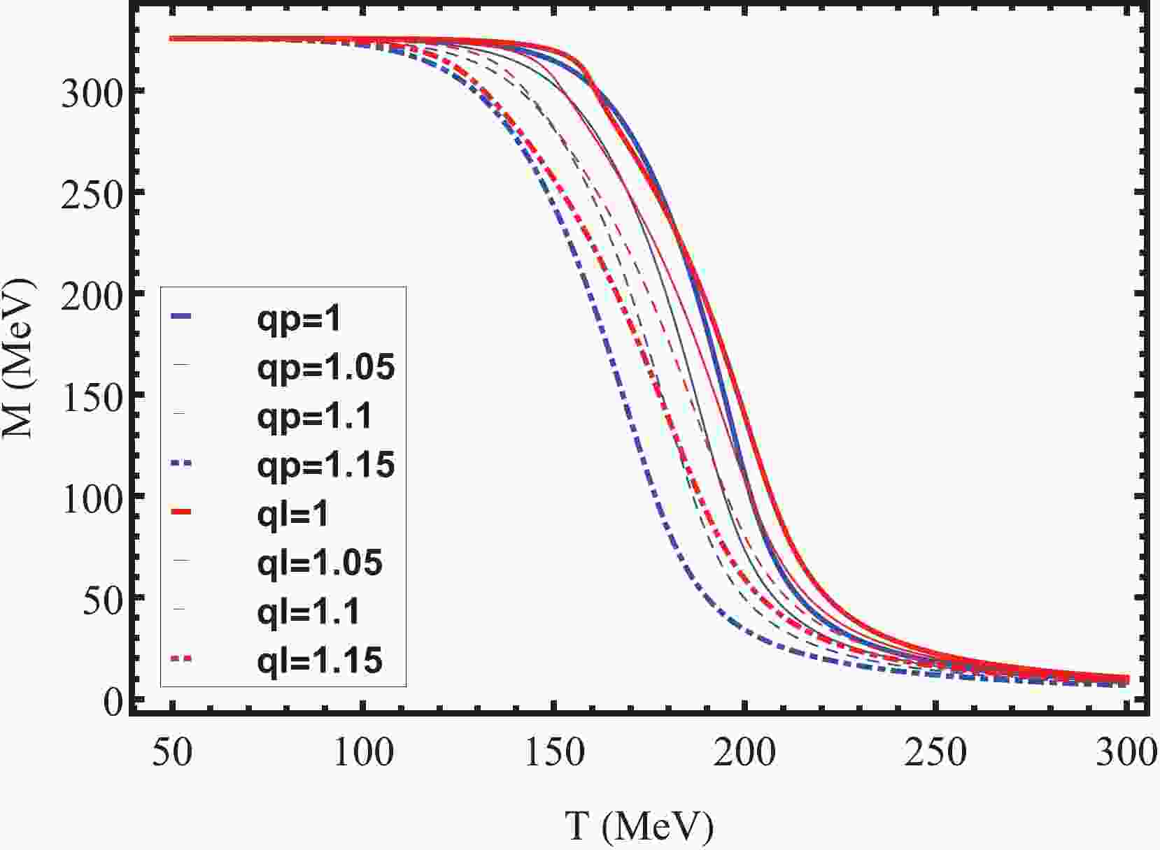
We plot M and
$ \Phi $ as a function of T for four different q, ($ q = 1 $ , 1.05, 1.1, 1.15) as well as two different$ \mathcal{U} $ ($ \mathcal{U_{P}} $ ,$ \mathcal{U_{L}} $ ), as shown in Figs. 1 and 2. We found that even considering the nonextensive effect, the finite-temperature QCD transition is still not a real phase transition but a crossover [45]. However, as q increases, the transition occurs at a smaller pseudo-critical temperature$ T_{c} $ . The same conclusion also appears in the nonextensive linear sigma model [9]. In addition, it is worth mentioning that the nonextensive effect has no influence on the QCD phase transition at zero temperature and finite chemical potential, as mentioned above.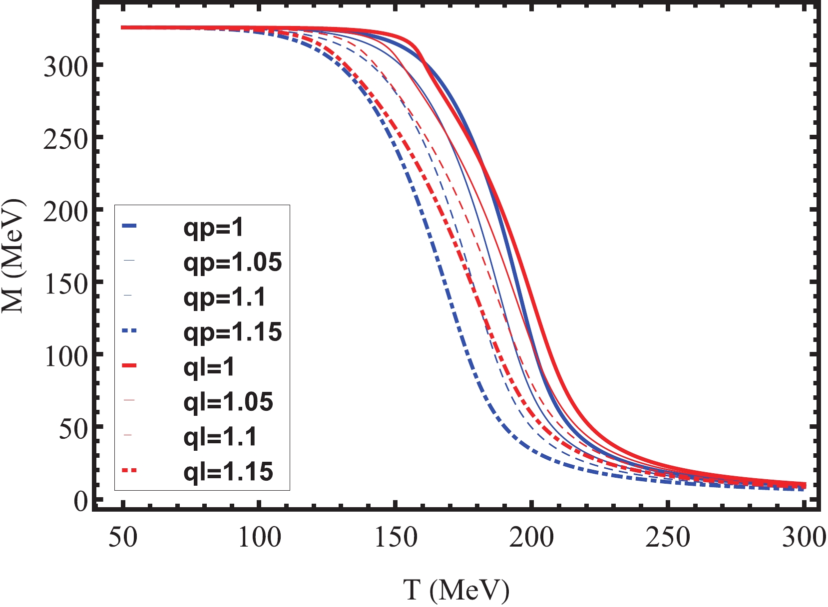
Figure 1. (color online) Constituent quark mass M as a function of T at
$\mu=0$ for two different potentials$\mathcal{U}$ and four parameters q, where$\mathrm{l}$ and${p}$ represent the logarithmic and polynomial Polyakov-loop potentials, respectively. The figure is taken from Ref. [40].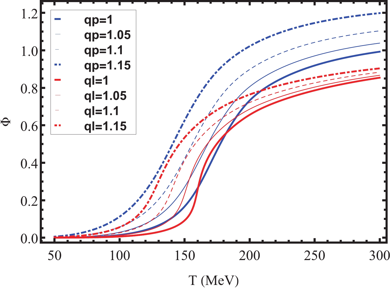
Figure 2. (color online) Polyakov-loop expectation value
$\Phi$ as a function of T at$\mu=0$ for two different Polyakov-loop potentials$\mathcal{U}$ and four parameters q. The figure is taken from Ref. [40].For small values of the chemical potential, the shape of the QCD crossover transition line can be characterized by its curvature, which is accessible to lattice QCD [46,47]. Therefore, next we discuss the influence of nonextensive effects on the curvature
$ \kappa $ . This is defined according to the Taylor series [48,49]:$ T_{c}(\mu) = T_{c}(0)(1-\kappa\mu^{2}/T_{c}^{2}(0)+O(\mu^{4}/T_{c}^{4}(0))), $

(26) and herein, we choose
$ \mu<100\ \mathrm{MeV} $ . The pseudo-critical temperature$ T_{c}(\mu) $ is determined by the peak of the thermal susceptibility, as follows [33]:$ \chi_{T} = \frac{\partial\sigma}{\partial T}. $

(27) For the Polyakov-loop potential
$ \mathcal{U_{P}} $ , the change in the crossover transition line with parameter q is shown in Fig. 3. We find that the pseudo-critical line gets lower and flatter with increasing q. In fact, the conclusion is the same for the Polyakov-loop potential$ \mathcal{U_{L}} $ . In order to better illustrate this, the change in curvature$ \kappa $ with q is listed in Table 4. Apparently,$ \kappa $ decreases as q increases. However, it should be noted that the curvature values we calculated are significantly higher than the values obtained in lattice QCD studies [46,47].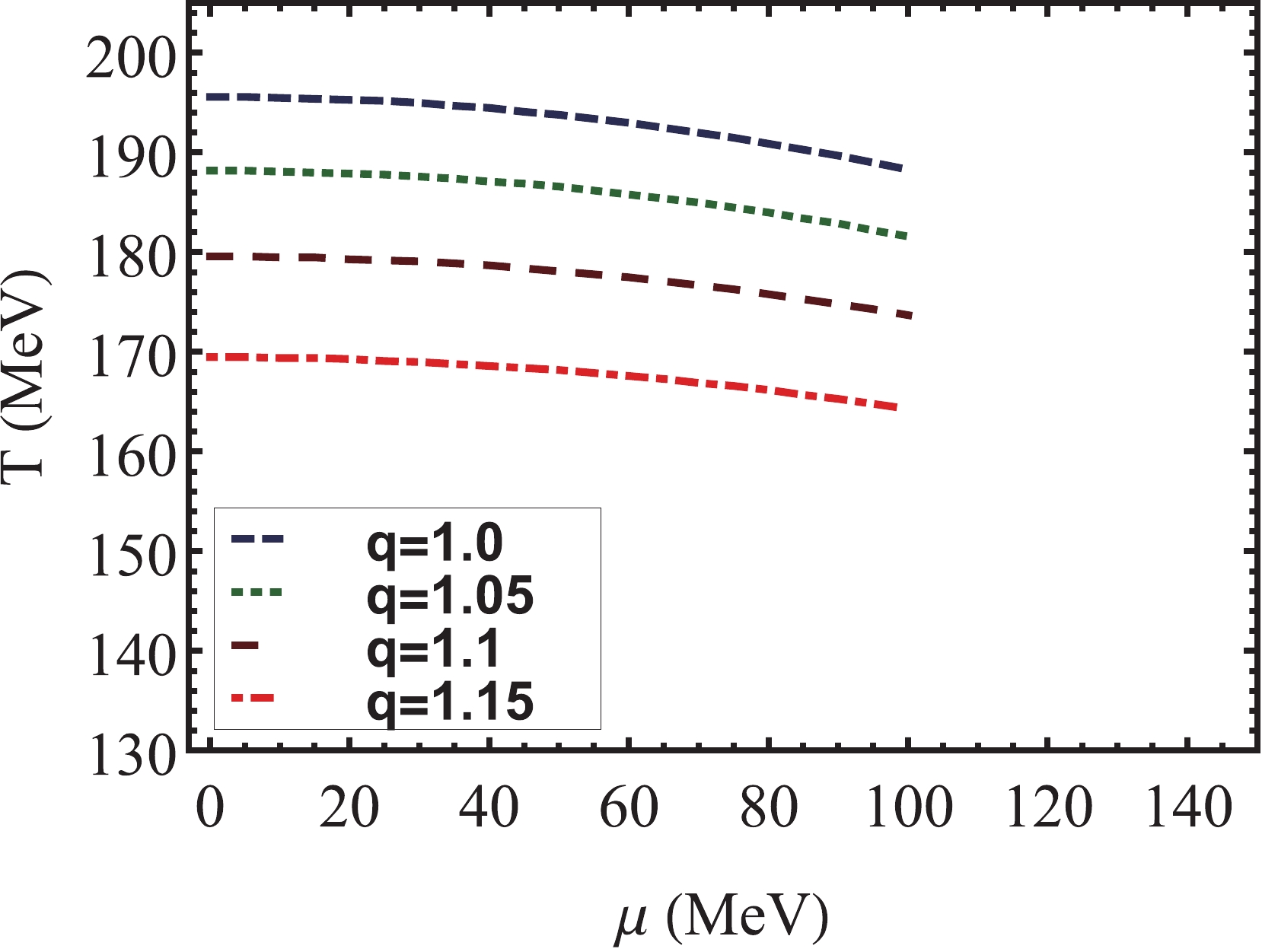
Figure 3. (color online) Variation of the pseudo-critical line with q, for Polyakov-loop potential
$\mathcal{U_{P}}$ .q 1 1.05 1.1 1.15 $\kappa_{P}$ 

0.142 0.124 0.106 0.090 $\kappa_{L}$ 

0.158 0.138 0.123 0.101 Table 4. Curvature
$\kappa$ changes with q, where$\kappa_{P}$ and$\kappa_{L}$ correspond to the Polyakov-loop potentials$\mathcal{U_{P}}$ and$\mathcal{U_{L}}$ , respectively.Finally, we are more concerned about the impact of the nonextensive effects on the CEP position. From Fig. 4, we clearly see that when
$ \mu = 329\ \mathrm{MeV} $ , the chiral condensation$ \sigma $ is discontinuous, which corresponds to a first-order phase transition. Moreover, when$ \mu = 327\ \mathrm{MeV} $ ,$ \sigma $ is continuous, which corresponds to a crossover transition. Therefore, there must be a critical termination point for the first-order phase transition line in the middle chemical potential region, which is CEP. As we know, in the neighborhood of the CEP position, the susceptibility tends to diverge. Taking$ q = 1 $ and the Polyakov-loop potential$ \mathcal{U_{P}} $ as an example, from Fig. 5, we can clearly see that when$ \mu = 328.1\ \mathrm{MeV} $ , the susceptibility shows quite a sharp and narrow divergent peak, which determines the position of CEP as$ (\mu_{c},T_{c}) = (328.1\ \mathrm{MeV},74.1\ \mathrm{MeV}) $ .
Figure 4. (color online) Chiral condensate
$\sigma$ as a function of T at$q=1$ for Polyakov-loop potential$\mathcal{U_{P}}$ and three different quark chemical potentials.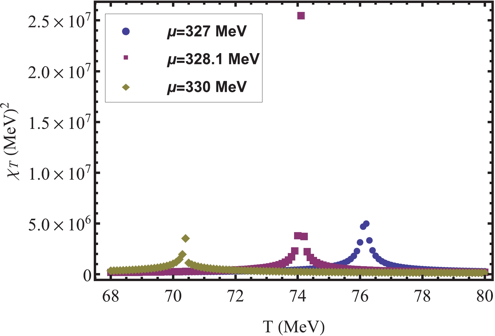
Figure 5. (color online) Susceptibility
$\chi_{T}$ as a function of T at$q=1$ for Polyakov-loop potential$\mathcal{U_{P}}$ and three different quark chemical potentials.The influence of the nonextensive effect on the position of CEP is shown in Figs. 6 and 7. We found that its impact on the position of CEP is not as simple as previously thought. As q increases, the CEP position moves in the direction of the larger chemical potential and lower temperature at first, but then, when q is larger than a critical value
$ q_{c} $ , the CEP position moves in the opposite direction. In other words, as q increases, CEP moves in the direction of the smaller chemical potential and higher temperature. Obviously, this interesting U-turn phenomenon is independent of the choice of Polyakov-loop potentials. For$ \mathcal{U_{L}} $ and$ \mathcal{U_{P}} $ , the critical values$ q_{c} $ are 1.1 and 1.08, respectively. It should be noted that this phenomenon was not found in Refs. [8,9]. Excluding the use of different models, one possible reason is that in Refs. [8,9], q was calculated only up to 1.1, which is just at the turning point. Our results are meaningful for the search of the CEP position in relativistic heavy-ion collision experiments. Based on our results, the search for areas with larger or smaller chemical potential depends on the critical value$ q_{c} $ .
Figure 6. (color online) Trajectory of CEP position with q in the T-
$\mu$ plane for Polyakov-loop potential$\mathcal{U_{L}}$ .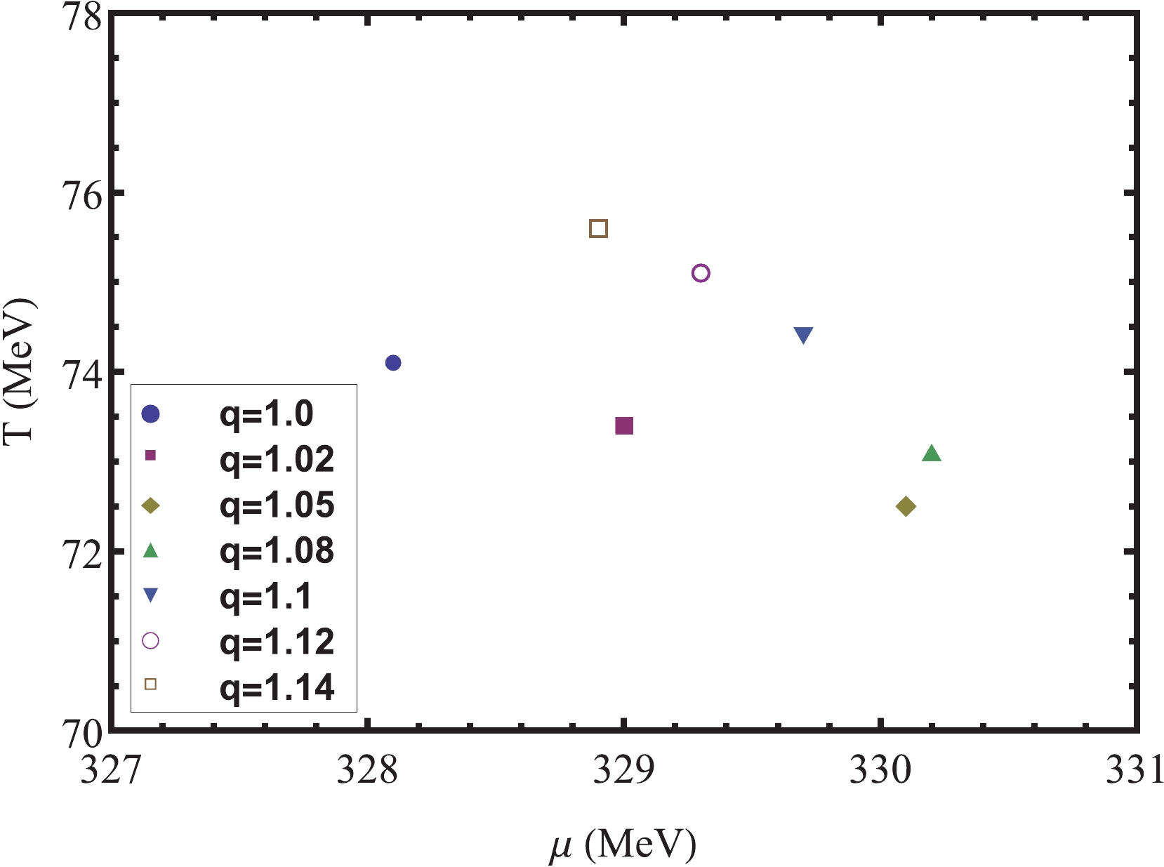
Figure 7. (color online) Trajectory of CEP position with q in the T-
$\mu$ plane for Polyakov-loop potential$\mathcal{U_{P}}$ . -
As we all know, in the vicinity of CEP, the divergence in susceptibility can be described by the critical exponents. Regarding the critical exponents, there are two important physical concepts: the scale hypothesis and the universality assumption. Regarding the scale hypothesis, its basic idea is that when approaching the critical point, the correlation length
$ \xi\rightarrow\infty $ , and the singularity of$ \xi $ determines the singularity of all thermodynamic functions. From this, the scaling law that should be satisfied between the critical exponents can be derived. Regarding the universality assumption, it refers to a system with the same spatial dimension d and order parameter dimension n, with the same critical exponent and belonging to the same universal category. However, it should be pointed out that the validity of these concepts is based on the equilibrium phase transition system described by BG statistics. Therefore, in a system that deviates from the description of BG statistics, the critical exponents may not be completely determined by d and n, and the scaling law may need to be reconstructed or modified [50-54]. Based on this, in this subsection, we use Tsallis statistics to study the critical exponents and discuss the influence of the nonextensivity parameter q on them. However, it should be pointed out that the critical exponents calculated below are mean-field values, due to the mean-field approximation employed in this work.Here, we choose a specific direction, which is denoted by
$ \uparrow $ ($ \downarrow $ ), for calculating the critical exponents using the path from lower (higher) T toward$ T^{\mathrm{C}} $ (represents$ T^{\mathrm{CEP}} $ ) with the quark chemical potential fixed at$ \mu^{\mathrm{C}} $ (represents$ \mu^{\mathrm{CEP}} $ ). Using the linear logarithmic fit, we obtain$ \mathrm{ln}\chi = -\gamma\mathrm{ln}|T-T^{C}|+c_{1}, $

(28) $ \mathrm{ln}|O-O^{C}| = \beta_{O}\mathrm{ln}|T-T^{C}|+c_{2}, $

(29) $ \gamma $ is the critical exponent of susceptibility, while$ \beta $ is the critical exponent of the order parameter O, and$ c_{1} $ ,$ c_{2} $ are constants. At$ q = 1 $ and in the direction$ \uparrow $ , the fitting procedure of the critical exponents for thermal susceptibility and quark mass is shown in Figs. 8 and 9.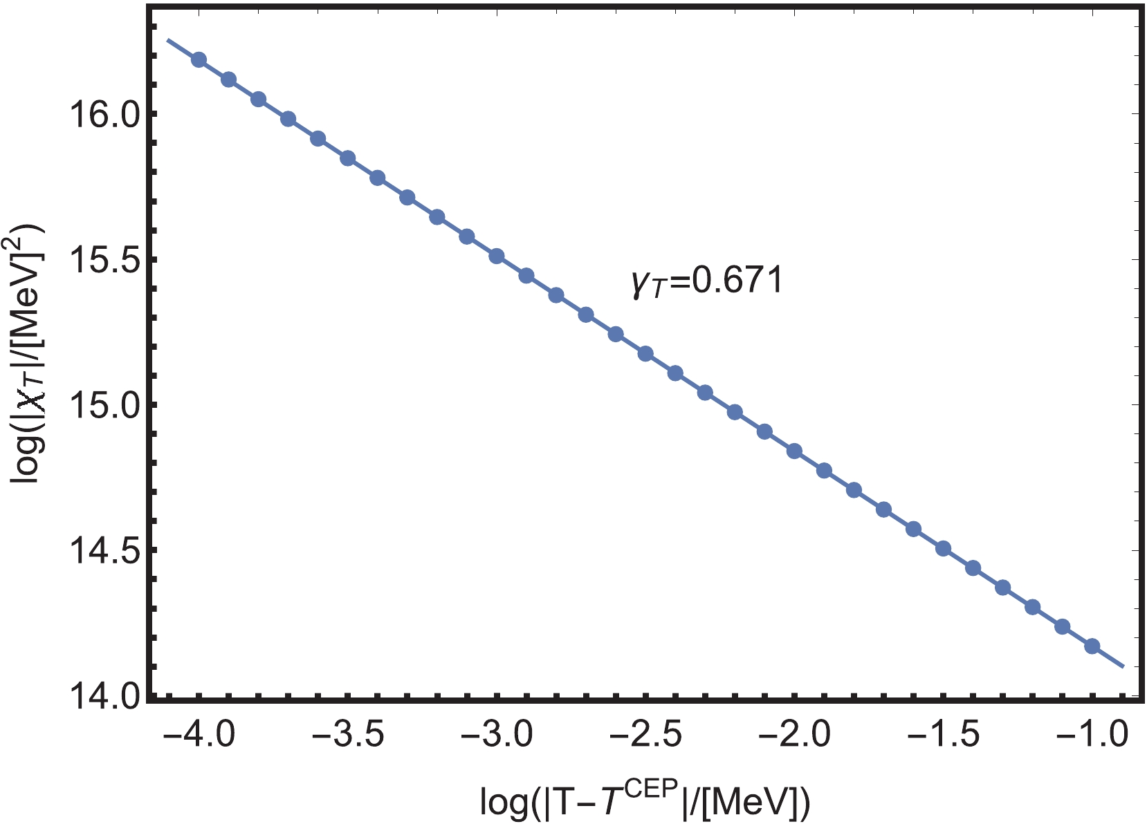
Figure 8. (color online) Logarithmic value of the thermal susceptibility
$\chi_{T}$ as a function of$\mathrm{log}|T-T^{\mathrm{CEP}}|$ at the fixed quark chemical potential$\mu^{\mathrm{CEP}}$ for Polyakov-loop potential$\mathcal{U_{P}}$ .
Figure 9. (color online) Logarithmic value of the quark mass M as a function of
$\mathrm{log}|T-T^{\mathrm{CEP}}|$ at the fixed quark chemical potential$\mu^{\mathrm{CEP}}$ for Polyakov-loop potential$\mathcal{U_{P}}$ .The variation in critical exponents with q is shown in Tables 5 and 6. We found that when q increases from 1.0 to 1.1, the critical exponent
$ \gamma_{T} $ remains almost unchanged, regardless of the Polyakov-loop potentials selected. However, for the critical exponent$ \beta $ , taking the Polyakov-loop potential$ \mathcal{U_{L}} $ as an example, we found that for the direction$ \uparrow $ ($ \downarrow $ ),$ \beta_{M} $ decreases (increases) with an increase in q. For the Polyakov-loop potential$ \mathcal{U_{P}} $ , this trend is the opposite. However, if we take the average value$ \bar{\beta}_{M} = (\beta_{M\uparrow}+\beta_{M\downarrow})/2 $ as the critical exponent parallel to the T axis, we find that$ \bar{\beta}_{M} $ is stable around 0.337 and hardly changes with q. In other words, even in Tsallis statistics, the critical exponents$ \gamma $ and$ \beta $ are still the same as their mean-field values$ \gamma = 2/3 $ and$ \beta = 1/3 $ in BG statistics [55-58].q Quantity Path Numerical result $q=1.0$ 

$\gamma_{T}$ 

$\uparrow$ 

0.677 $\downarrow$ 

0.678 $\beta_{M}$ 

$\uparrow$ 

0.361 $\downarrow$ 

0.309 $q=1.05$ 

$\gamma_{T}$ 

$\uparrow$ 

0.680 $\downarrow$ 

0.685 $\beta_{M}$ 

$\uparrow$ 

0.332 $\downarrow$ 

0.346 $q=1.1$ 

$\gamma_{T}$ 

$\uparrow$ 

0.681 $\downarrow$ 

0.679 $\beta_{M}$ 

$\uparrow$ 

0.315 $\downarrow$ 

0.362 Table 5. Dependence of the critical exponents on the nonextensivity parameter q for Polyakov-loop potential
$\mathcal{U_{L}}$ .q Quantity Path Numerical result $q=1.0$ 

$\gamma_{T}$ 

$\uparrow$ 

0.671 $\downarrow$ 

0.678 $\beta_{M}$ 

$\uparrow$ 

0.318 $\downarrow$ 

0.353 $q=1.05$ 

$\gamma_{T}$ 

$\uparrow$ 

0.668 $\downarrow$ 

0.683 $\beta_{M}$ 

$\uparrow$ 

0.364 $\downarrow$ 

0.307 $q=1.1$ 

$\gamma_{T}$ 

$\uparrow$ 

0.660 $\downarrow$ 

0.673 $\beta_{M}$ 

$\uparrow$ 

0.370 $\downarrow$ 

0.304 Table 6. Dependence of the critical exponents on the nonextensivity parameter q for Polyakov-loop potential
$\mathcal{U_{P}}$ .It is worth noting that, in Ref. [50], the critical behavior of a two-dimensional Ising model with nonextensive statistics was studied, and it was found that for
$ 0.5<q<1 $ , the critical exponents$ \alpha $ ,$ \beta $ , and$ \gamma $ depend on q in the form$ \alpha(q) = (10q^{2}-33q+23)/20 $ ,$ \beta(q) = $ $ (2q-1)/8 $ , and$ \gamma(q) = (q^{2}-q+7)/4 $ . However the critical exponent$ \nu $ does not depend on q. Using the same model, in Ref. [51], it was found that although the critical exponent$ \beta $ is different from its value in BG statistics, it does not depend on q within the margin of error. In particular, the critical exponent$ \nu $ depends on q in a linear manner. At present, the impact of the nonextensive effect on the critical exponent, especially for the two cases of$ q<1 $ and$ q>1 $ , is not very clear. Therefore, it is worthy of further research. -
In this paper, combined with the Tsallis statistics and the PNJL model, we investigated the sensitivity of the QCD phase transition and critical exponents with regard to deviations from usual BG statistics. Regarding the QCD phase diagram, we found that the influence of nonextensive effects on the CEP position shows a very interesting U-turn phenomenon. At the beginning, with an increase in q, the CEP position moves toward the direction of larger chemical potential and lower temperature. However, when q is larger than a critical value
$ q_{c} $ , as q increases, the CEP position moves in the opposite direction, that is, in the direction of smaller chemical potential and higher temperature. Because of this U-turn phenomenon, we found that searching for CEP in larger or smaller chemical potential regions in relativistic heavy-ion collisions depends on a critical value$ q_{c} $ . This is a very interesting result that deserves further study. Regarding the critical exponents, numerical results based on Tsallis statistics show that the critical exponents remain almost constant with q. In other words, different from the findings in Refs. [50,51], we found that the critical exponents do not depend on the choice of Tsallis statistics or BG statistics. In addition, quark stars, as candidates for observed massive stars ($ \geqslant 2M_{\odot} $ ), have attracted much attention in astronomy [4,59-61]. Therefore, studying the influence of nonextensive effects on the structure and evolution of protoquark stars is a very meaningful topic. We shall study these issues in future.
QCD chiral phase transition and critical exponents within the nonextensive Polyakov-Nambu-Jona-Lasinio model
- Received Date: 2020-10-29
- Available Online: 2021-07-15
Abstract: We present a nonextensive version of the Polyakov-Nambu-Jona-Lasinio model that is based on nonextentive statistical mechanics. This new statistics model is characterized by a dimensionless nonextensivity parameter q that accounts for all possible effects violating the assumptions of the Boltzmann-Gibbs (BG) statistics (for


 DownLoad: