


 Abstract
 HTML
HTML Reference
 Related
 PDF
PDF


-
Vector Boson Scattering (VBS) represents sensitive probe of both the Standard Model (SM) electroweak symmetry breaking (EWSB) and new beyond-the-SM (BSM) physics [1, 2]. If the couplings between the Higgs and vector bosons deviate from the SM prediction, the cross-sections of VBS processes will increase with center-of-mass energy up to the scale of new physics. In addition, many BSM models predict an extended Higgs sector. The contribution from new resonances can also increase the VBS cross-section in certain phase spaces.
Measuring VBS processes at hadron collider is experimentally challenging, owing to their low signal yields and complex final states. The LHC experiments have performed comprehensive searches for VBS processes [3-5]. The same-sign
$ WW $ production with leptonic decay has the largest signal-to-background ratio among VBS processes. This channel was the first VBS process to be observed during Run I of the LHC [6, 7] and has been confirmed by measurements from the LHC's Run II [8, 9]. The ATLAS and CMS Collaborations have also measured other VBS channels, including fully leptonic$ ZZ $ [10, 11], fully leptonic$ WZ $ [12, 13], and semi-leptonic$ WV $ or$ ZV $ with the V decaying hadronically [14, 15]. New physics contributions to the VBS channels are usually parameterized by effective field theory (EFT) operators. Precise measurement of the VBS channels can be recast as constraints on the coefficients of the operators [16-18].Understanding the polarization of the gauge bosons is an important step following measurements of the VBS processes. Vector bosons are unstable and can only be observed via their decay products. This generates interference between different polarizations, which exactly cancels only when the azimuthal angles of the decay products are integrated over. Even though selection cuts in analyses render the cancellation incomplete, it remains possible to extract polarization fractions by fitting the data with Monte-Carlo-simulated templates. Studies have sought to determine the polarization of gauge bosons in the
$ W^\pm W^\mp $ channel [19, 20], fully leptonic$ W^\pm W^\pm $ channel [21], fully leptonic WZ/ZZ channels [22], the SM Higgs decay [23], and generic processes featuring boosted hadronically decaying W bosons [24]. Various kinematic observables have been proposed in these works to discriminate between the longitudinally and transversally polarized gauge boson. Several recent studies have shown that deep neural networks inputted with the final states' momenta can be used for regression of the lepton angle in the gauge boson rest frame [25, 26] and to classify events from different polarizations [27, 28].Autoencoders have been widely used in model-agnostic searches at colliders (referred to as anomaly detection or novelty detection). The main function of the autoencoder is to learn to map an input to a latent compressed representation and then back to itself. An autoencoder trained on known SM processes can identify BSM events as anomalies [29-36]. In other cases, when the anomaly can not be detected on a single event, density-based novelty evaluators [37-39] are used to detect discrepancies between two datasets in the latent space. Because the VBS processes are ideal probes for accessing any new physics relating to EWSB, we adopt autoencoders to detect possible new physics contributions to this process.
In this work, by focusing on the fully leptonic and semi-leptonic channels of the
$ W^\pm W^\mp $ +jets process, we propose a neural network based on the transformer architecture [40], to learn the features of the VBS process. These features are not only useful for separating the VBS process from the SM backgrounds but also capable of discriminating between different polarizations of the W bosons in the VBS process. An autoencoder is trained on features to reduce the dimensionality such that only the most relevant features are retained. Eventually, we perform a binned log-likelihood test in the latent space, to determine whether the feature distributions coincide with the SM prediction. The EFT and Two Higgs Doublet Model (2HDM) are considered as examples, to demonstrate that the method can test a wide range of BSM physics.The paper is organized as follows: in Sec. II, the analysis framework is introduced, including the event generation, neural network architecture, and binned log-likelihood analysis; in Sec. III, the discrimination of different polarization modes of the
$ WWjj $ production is discussed; in Secs. IV and V, we consider the application of our method to the EFT and 2HDM, respectively; our conclusions are presented in Sec. VI. -
The signal and background events in our study are generated using the MADGRAPH5_AMC@NLO [41] framework, in which the MADSPIN is used for the decays of heavy SM particles (top quark, W/Z boson), and PYTHIA 8.2 [42] is used for the parton shower, hadronization, and hadronic decay. The latest version of MG5 is capable of handling polarized parton scattering [43]. This function is adopted to simulate the events of VBS processes exhibiting fixed vector boson polarization in the final state. The detector effects are simulated by DELPHES 3 with the ATLAS configuration card, where the b-tagging efficiency is set to 70%, and the mistagging rates for the charm- and light-flavor jets are 0.15 and 0.008, respectively [44]. The clustering of final state particles into jets is implemented by FASTJET [45] using the anti-
$ k_T $ algorithm with cone-size parameter$ R = 0.4 $ .All of the diagrams at
$ \alpha_{\text{EW}}^4 $ ($ \alpha_{\text{EW}} $ is the electroweak coupling constant) are included in simulations of the VBS process (hereafter referred to as EW production), including$ \gamma \gamma \to WW $ processes with the final state vector boson radiated from quark directly, as well as the significant interferences between diagrams. Mixed electroweak--quantum chromodynamics (QCD) di-boson productions are also present at$ \mathcal{O}(\alpha_s^2 \alpha^2_{\text{EW}}) $ , where$ \alpha_s $ is the strong coupling constant. In the SM, the interference between the electroweak and mixed EW--QCD production is small [20, 46, 47]. When simulating the polarized processes, the definition of the polarization is frame-dependent. In this work, we take the partonic center of mass frame as the reference (i.e., the rest frame defined by the two initial parton in the$ q q'\to W^+ W^- j j $ process①).We study both the di- and semi-leptonic channels of the EW
$ W^\pm W^\mp jj $ production. Thus, at least one of the W bosons should decaying leptonically (denoted by$ W_\ell W jj^{\text{EW}} $ ). The dominant backgrounds are the QCD production of the$ t\bar{t} $ process, single-top production, mixed EW--QCD production of$ WW/WZ $ , and the EW production of$ WZ $ . Because the fully hadronic final states are irrelevant to our analysis, the following requirements are applied to generate the background events: (1) at least one of the tops decays leptonically in the$ t\bar{t} $ process (denoted by$ t t_\ell $ ), (2) either a W or top quark decays leptonically in the$ tW $ process (denoted by$ tW_\ell/t_\ell W $ ), (3) at least one of the W boson decays leptonically in the mixed electroweak--QCD$ WWjj $ process (denoted by$ W_\ell Wjj^{\text{QCD}} $ ), (4) the W boson decays leptonically in the mixed electroweak--QCD$ WZjj $ process (denoted by$ W_\ell Zj j^{\text{QCD}} $ ) and in the EW$ WZjj $ process (denoted by$ W_\ell Z j j^{\text{EW}} $ ). In all cases, the transverse momenta of final state jets should exceed 20 GeV. We use the measured inclusive cross-sections at the LHC for$ t\bar{t} $ [48] and$ tW $ [49] processes, and we use the leading-order cross-sections calculated by MADGRAPH5_AMC@NLO for di-boson processes. The fiducial cross-sections at 13 TeV (LHC) are presented in the second column of Table 1.$ \sigma^{\text{fid}} $ /pb

$ \sigma^{\ell \ell} $ /fb

$ \sigma^{\ell j} $ /fb

$ t t_\ell $ 

210.3 139.8 3007.6 $ t W_\ell $ /

$ t_\ell W $ 

15.9 11.6 224.6 $ W_\ell W j j^{\rm{QCD}} $ 

4.68 14.7 340.5 $ W_\ell Z j j^{\rm{QCD}} $ 

2.20 4.49 165.7 $ W_\ell Z j j^{\rm{EW}} $ 

0.487 3.68 22.2 $ W_\ell Wj j^{\rm{EW}} $ 

0.738 4.36 37.3 Table 1. Production cross-sections of signal and background processes before and after pre-selections.
The events are divided into two classes with the following preselections [3]:
● Di-lepton: exactly two opposite-sign leptons with
$ p_T(\ell) >20\; \text{GeV}, \; |\eta(l)|<2.5 $ ; at least two jets with$ p_T(j) >20\; \text{GeV}, \; |\eta(j)|<4.5 $ ; the two jets with leading$ p_T $ should produce large invariant mass ($ m_{jj}>500 $ GeV) and have a large pseudorapidity separation ($ |\Delta \eta|_{jj}>3.6 $ ); no b-tagged jet in the final state.● Semi-lepton: exactly one charged lepton with
$ p_T(\ell) >20\; \text{GeV}, \; |\eta(l)|<2.5 $ ; at least four jets with$ p_T(j) >20\; \text{GeV}, \; |\eta(j)|<4.5 $ ; the pair of jets with the largest invariant mass ($ m_{jj}>500 $ GeV) that also satisfies$ |\Delta \eta|_{jj}>3.6 $ is taken as the forward-backward jet pair; (4) of the remaining jets, that with an invariant mass closest to the W boson mass is regarded as the jet pair from the W decay.The cross-sections for signal and backgrounds after the Di-Lepton and Semi-Lepton selections are provided in the third and fourth columns of the Table 1, respectively. We find that the
$ t\bar{t} $ process is the most important background in both channels; its cross-section is$ \sim \mathcal{O}(100) $ times larger than that of the VBS process.The preselected events are fed into the network for feature learning. The deep learning is understood to be able to transform lower-level inputs into discriminative outputs. Thus, we represent each event by a set of four-momenta② and their identities (the lepton charge is implied). Different networks are adopted for the di- and semi-leptonic channels. The inputs for the dileptonic channel network consists of the momenta of two leptons, forward and backward jets, the sum of all detected particles, and the sum of jets not assigned as forward-backward jets. Furthermore, the input for the semi-leptonic channel network consists of the momenta of the lepton, forward and backward jets, two jets from the W decay, the sum of all detected particles, and the sum of remaining jets③. In short, there are six/seven momenta (with identities) for the inputs of the di-/semi-leptonic channel.
-
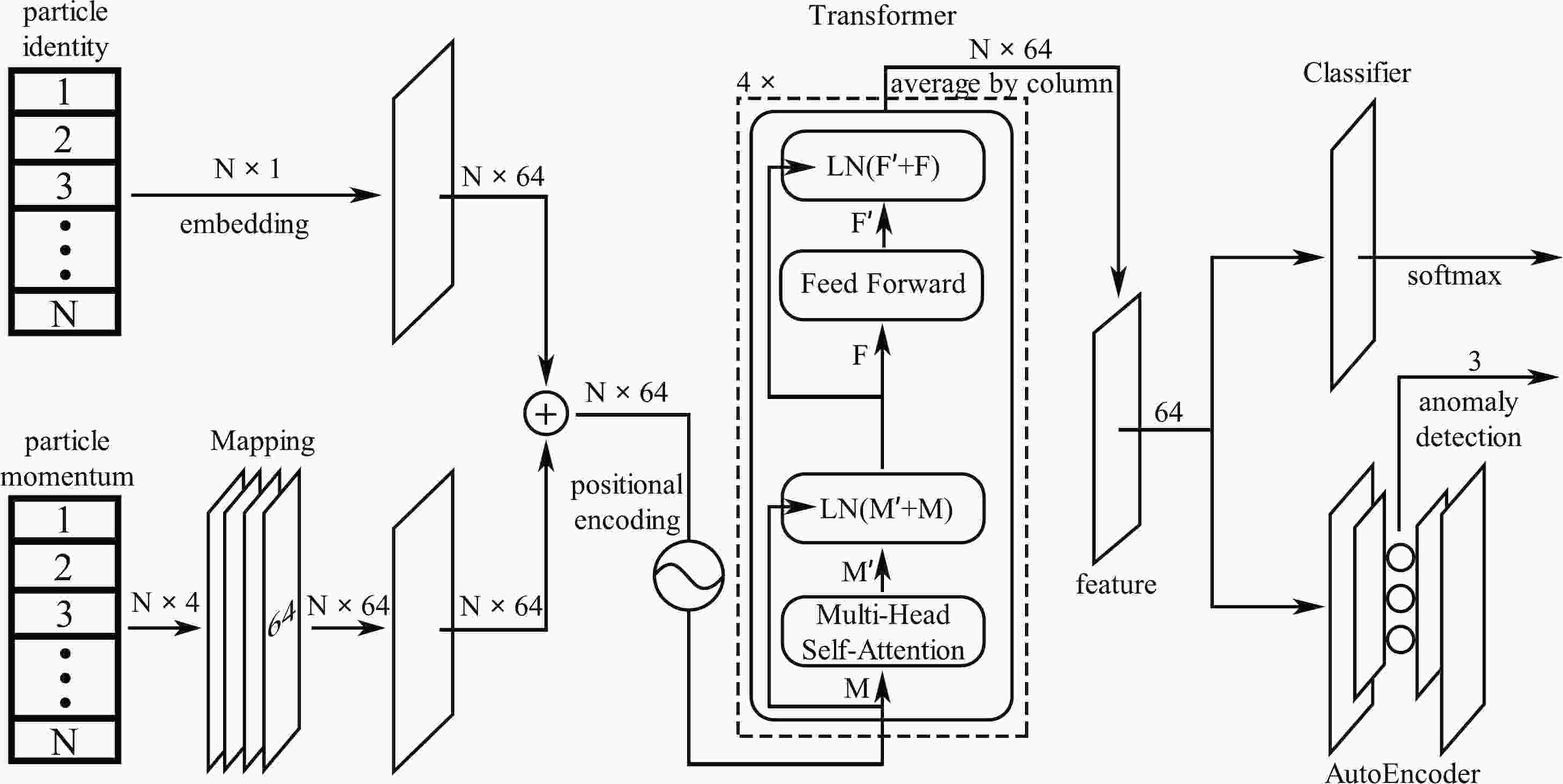
A simple fully connected neural network can extract the features of the input data; however, it produces numerous redundant connections, which reduces the extraction efficiency and increases the likelihood of overfitting. These problems can be alleviated by including an attention mechanism. As proposed in Ref. [40], a transformer with a multi-head self-attention mechanism provides a variety of different attentions and improves the learning ability; thus, it can be used to effectively extract the internal feature connections.
The architecture of our neural network is illustrated in Fig. 1. The input consists of identities and the four-momenta of N particles (
$ N = 6/7 $ for the di-/semi-leptonic channel). The original particle's momentum ($ p^{\mu} $ ) is normalized according to
Figure 1. Neural network architecture.
$ \hat{p}^{\mu}_{i} = \frac{p^{\mu}_{i} - \bar{p}^\mu} {\sigma_{p^{\mu}}}, $

(1) where the index i runs over the N particles in an event. The mean
$ \bar{p}^\mu $ and standard deviation$ \sigma_{p^{\mu}} $ are calculated for particles from the full set of the training sample. Then, we embed the particle identities of each event into a uniform distribution ($ N \times 64 $ ) and map the normalized four-momenta to a matrix ($ N\times64 $ ) via a mapping network. The mapping network is a fully connected neural network with four hidden layers (each layer contains 64 neurons). The sum of these two components (which encode the particle types into the four-momenta, denoted by$ M_{N\times 64} $ ) is fed into the transformer. The transformer contains four copies of the encoder layers. Each encoder consists of a self-attention layer and a feedforward neural network followed by normalization layers. In particular, the self-attention layer maps the$ M_{N\times 64} $ into$ M'_{N\times 64} $ $ \begin{aligned}[b] M'_{N\times 64} = &\bigg[\text{Softmax}\left(\frac{W^Q_1 (W^K_1)^T}{8 }\right) W^V_1, \cdots ,\\&\text{Softmax}\left(\frac{W^{Q}_4 (W^K_4)^T}{8 }\right) W^V_4 \bigg]_{N\times 64} \cdot W^{\prime O}_{64 \times 64}\; , \end{aligned} $

(2) where
$ W^{Q,K,V} $ is constructed from$ M_{N\times 64} \cdot W^{\prime Q,K,V}_{64 \times 16} $ and$ W^{\prime Q,K,V,O} $ are trainable parameter matrices.The output of the transformer is a matrix of size
$ N\times64 $ . The features are obtained by averaging over the particle index (which gives it the shape$ 1 \times 64 $ ). Finally, a classifier and autoencoder are applied to classify the inputs (according to the processes to which they belong) and reduce the dimensionality of the feature space. The classifier and autoencoder are trained simultaneously, using an Adam optimizer with a learning rate of$ 3 \times 10^{-4} $ . Although higher-dimensional feature spaces provides better discriminative power, the statistical uncertainty of the shape analysis is significantly larger owing to the limited number of simulated events [$ \mathcal{O}(10^{5}) $ for each signal process after preselection]. In Fig. 2, we show the stabilized loss (typically measured after$ \sim $ 100 epochs of training) of the autoencoder for different choices of feature-space dimensionality. For all polarization modes in the di- and semi-leptonic channels, the three-dimensional latent space can reproduce the 64-dimensional features reasonably well (with losses of$ \lesssim 10^{-4} $ ). Meanwhile, binned log-likelihood analysis can be performed with a relatively small statistical uncertainty.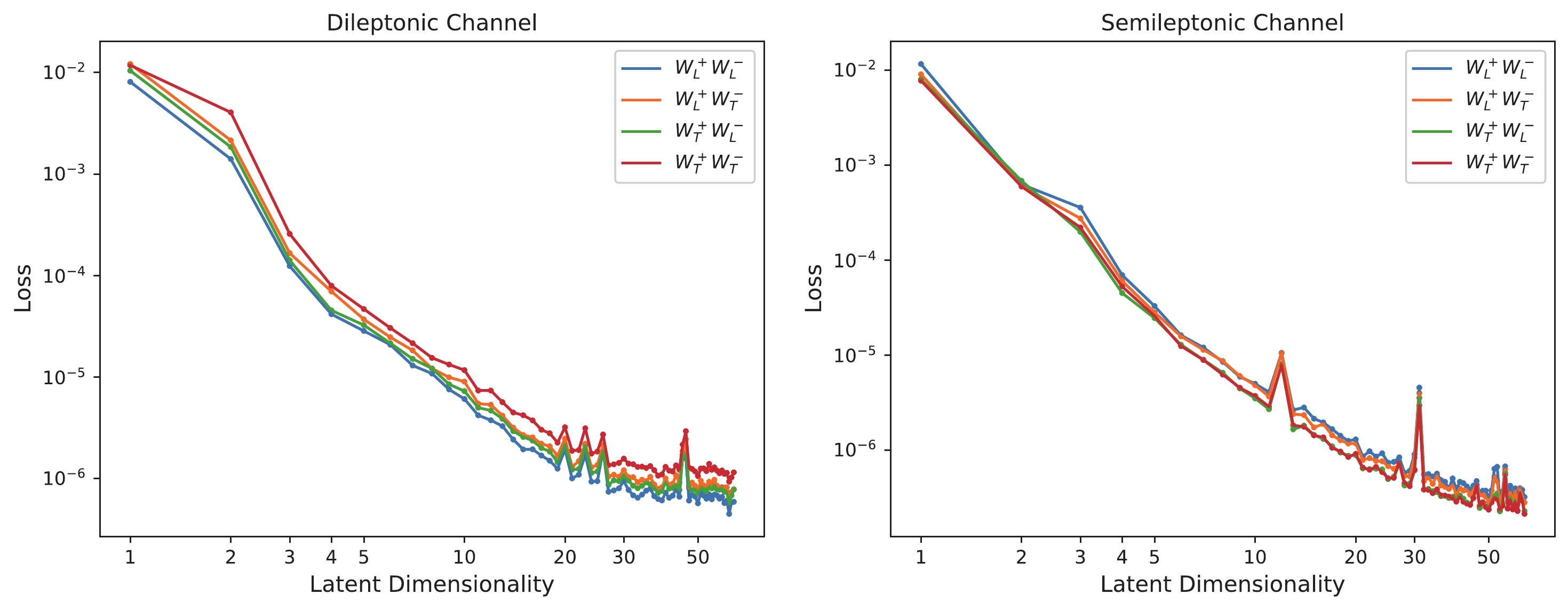
Figure 2. (color online) Stabilized loss of the autoencoder for different choices of feature-space dimensionality in the di- (left panel) and semi- (right panel) leptonic channels.
-
The three-dimensional latent space is divided into
$ 8 \times 8 \times 8 $ and$ 10 \times 10 \times 10 $ bins for the di- and semi-leptonic channels, respectively, because the latter has a larger production rate. In principle, one could perform the binned log-likelihood test over all bins; however, this renders the result sensitive to the tail of the distribution when the signal and background event numbers are small. Although more dedicated analysis can resolve this issue, we use only bins that contain relatively large numbers of signal events, for simplicity. Of the bins that contain at least 1% of the total signal events, the ten with the highest signal-to-background ratios are selected for the log-likelihood test④. Here, the background refers to the summed contributions of the$ t t_\ell $ ,$ t W_\ell $ /$ t_\ell W $ ,$ W_\ell Wjj^{\text{QCD}} $ ,$ W_\ell Z jj^{\text{QCD}} $ , and$ W_\ell Z jj^{\text{EW}} $ processes. Furthermore, the signal refers to the$ W_\ell W jj^{\text{EW}} $ and its new physics modifications. In realistic experiments, the number of signals in each bin can be obtained by subtracting the predicted background event number from the measured one. This procedure selects$ \sim $ 30% of the signal events and$ \sim $ 0.5% of the total background events in most cases. According to the cross-sections in Table 1, this procedure reduces the cross-section of the combined backgrounds to the same level as that of the VBS signal.For a given hypothesis
$ \mathcal{H} $ (either the SM or new physics BSM), the expected number of events ($ t_i $ ) in the i-th bin can be obtained from Monte Carlo simulations. The likelihood of the i-th bin featuring$ n_i $ observed events follows a Poissonian probability,$ t_i^{n_i} {\rm e}^{-t_i} / n_i ! $ . Thus, we can determine the probability for the full distribution by multiplying the Poissonian probabilities of the selected bins. The binned likelihood for hypothesis$ \mathcal{H}_\alpha $ is defined as$ \mathcal{L}(\text{data}| \mathcal{H}_\alpha) = \prod\limits_{i} \frac{t_i^{n_i} {\rm e}^{-t_i} }{n_i!}, $

(3) where i runs over the ten selected bins. Subsequently, we can define the test statistic
$ \mathcal{Q} $ as the log-likelihood ratio between a given hypothesis$ \mathcal{H}_\alpha $ (i.e., new physics with fixed parameters) and the null hypothesis$ \mathcal{H}_0 $ (the SM):$ \mathcal{Q} = -2 \log \left( \frac{\mathcal{L}(\text{data}| \mathcal{H}_\alpha)}{\mathcal{L}(\text{data}| \mathcal{H}_0 )} \right). $

(4) We use the predicted numbers of events from the two hypotheses (
$ \mathcal{H}_\alpha $ and$ \mathcal{H}_0 $ ) to generate two sets of pseudo-data. In each bin, the pseudo-data are obtained by generating a random number from the Poissonian distribution (statistical uncertainty) + Gaussian distribution (systematical uncertainty) with a mean value of$ t_i $ . We repeat this procedure$ 10^6 $ times for$ \mathcal{H}_\alpha $ and$ \mathcal{H}_0 $ . This gives two distributions of the test statistic$ \mathcal{Q} $ . Finally, the p-value of the test hypothesis ($ \mathcal{H}_{\alpha} $ ) can be calculated by assuming that, under the null hypothesis, the actual observation is at the center of the$ \mathcal{Q} $ distribution. -
Of the polarization modes of the VBS processes, the longitudinally polarized component is most closely related to the unitarity problem (i.e. the properties of the Higgs boson) and possible new physics. Numerous studies have sought to separate the polarization of the gauge boson in the VBS process, by exploiting various kinematic variables. The lepton angular distribution in the gauge boson rest frame is understood to be sensitive to the vector boson polarization, expressed as
$ \frac{1}{\sigma} \frac{{\rm d} \sigma}{{\rm d} \cos \theta} = \frac{3}{8} f_L (1+\cos \theta)^2 + \frac{3}{8} f_R (1-\cos \theta)^2 + \frac{3}{4} f_{0} \sin^2 \theta, \; $

(5) where the
$ f_{L,R,0} $ is the fraction of the corresponding helicity and$ \theta $ is the angle between the vector boson flight direction in a certain frame and the lepton flight direction in the vector boson rest frame. Even though the shape of the angular distribution represents a good discriminating variable, it often cannot be reconstructed precisely. The dileptonic channel of$ W^\pm W^\mp jj $ contains two missing neutrinos in the final state. We cannot reconstruct the rest frame for individual W bosons. In the semi-leptonic channel, even though the neutrino momentum can be solved up to a twofold ambiguity (and thus the full momenta of all particles can be calculated), large uncertainties are typically involved when measuring the jets' momenta and identifying the forward-backward and W-boson-decay-produced jets. Moreover, the shape of the$ \theta $ distribution can be distorted by the kinematic cuts used to separate the VBS from its background [50].In this section, we demonstrate that our network is capable of discriminating different polarization modes of the electroweak
$ W^\pm W^\mp jj $ production from low-level inputs. -
We train the network with labeled events of electroweak
$ W^+_L W^-_L jj $ ,$ W^+_L W^-_T jj $ ,$ W^+_T W^-_L jj $ , and$ W^+_T W^-_T jj $ productions, respectively. Here,$ W_L $ ($ W_T $ ) represents the longitudinally (transversely) polarized W boson. The normalized⑤ distributions of these polarization modes in the three-dimensional latent space are shown in Fig. 3. Larger cubes indicate more events in that bin. We can identify remarkable differences between the distributions of different polarizations.
Figure 3. (color online) Normalized distributions of the latent features for different polarization modes in the dileptonic channel.
To assess the discriminative power of our network, we perform a comparative study on methods using different input variables. Besides the three latent features, two classes of variables are defined⑥:
● Detector-level variables: Variables in this class can be reconstructed experimentally; they include the transverse momenta of two leptons
$ p_T (\ell_{1,2}) $ and forward-backward jets$ p_T(j_{1,2}) $ , and the azimuthal angle difference between the forward and backward jets$ \Delta \phi(j,j) $ .● Truth-level variables: Variables in this class can only be obtained from Monte Carlo simulations; they include the transverse momenta of two W bosons
$ p_T(W^\pm) $ and the lepton angle in the W boson rest frame$ \cos(\theta_{l^\pm}) $ . The later is calculated from$ \cos \theta = \dfrac{\vec{p}_W \cdot \vec{\tilde{p}}_\ell}{|\vec{p}_W| |\vec{\tilde{p}}_\ell |} $ , where$ \vec{p}_W $ is the W boson momentum in the initial parton center of mass frame and$ \vec{\tilde{p}}_\ell $ is the lepton momentum in the W boson rest frame.The Gradient Boosting Decision Tree (GBDT) method is adopted to calculate the receiver operating characteristic (ROC) curves for input variables in a class either with or without the latent variables. The ROC curves are shown in the left-hand panel of Fig. 4, where we have considered the
$ W^+_L W^-_L jj $ events as the signal and the events of other polarization modes as background. Methods using latent features alone have already outperformed the GBDT for all detector-level variables. Furthermore, a GBDT that combines the latent variables with detector-level ones does not offer a better discriminative power than the method using latent variables alone. This indicates that information regarding these detector-level variables should be included in the latent variables. The GBDT using truth-level variables offers a slightly improved discriminative power than the method with latent variables. Interestingly, the discriminative power can be improved further by combining the truth-level and latent variables.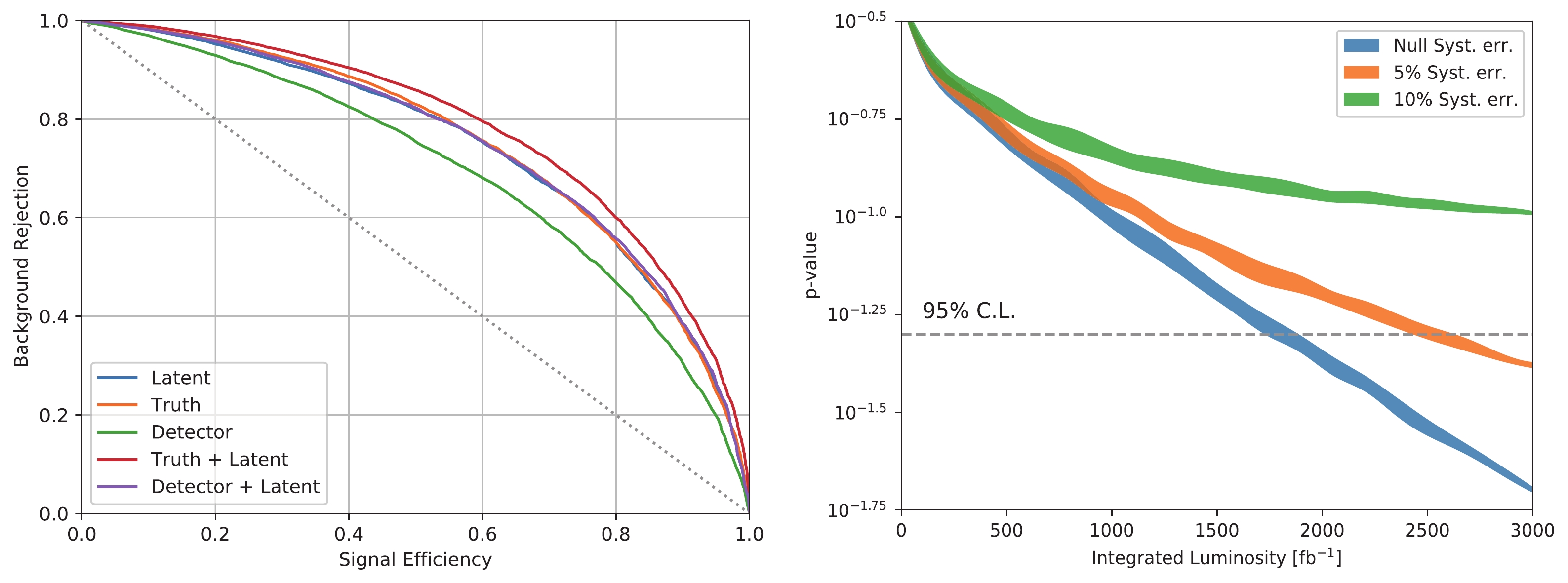
Figure 4. (color online) Left: comparison of the discriminative powers of methods using different input variables in the dileptonic channel. Right: sensitivity to a 1% change in the rate of the
$ W^+_L W^-_L jj $ mode; the band width indicates the statistical uncertainty, and the colors denote different systematic uncertainties.When the new physics modifies the Higgs--gauge boson interaction, the incomplete cancellation of the VBS amplitude increases the fraction of longitudinally polarized gauge boson final states. The current precision measurements of the SM permit the
$ W^+_L W^-_L jj $ fraction to be increased by a single percentage (e.g., from 6 to 7% in the following case). To study the sensitivity of latent variables to this increment of change, we perform binned log-likelihood analysis, taking the SM cross-section (after applying the cut of$ m_{jj}>500 $ GeV at parton level) for each polarized component. These are$ \sigma(W^+_L W^-_L) = 25.5 $ fb,$ \sigma(W^+_L W^-_T) = 73.2 $ fb,$ \sigma(W^+_T W^-_L) = $ $ 76.9 $ fb, and$ \sigma(W^+_T W^-_T) = 243.8 $ fb, respectively. The test hypothesis takes$ \sigma(W^+_L W^-_L) = 29.7 $ fb whilst keeping other cross-sections identical. The p-values for the hypothesis test under varying integrated luminosity are shown in Fig. 4, where we have considered the cases with three different systematic uncertainties. We can conclude that the future LHC will be capable of detecting such changes, provided the systematic uncertainty is below$ \sim $ 5%. Note that the background processes are negelcted at this stage. Moreover, the new physics cannot be simply considered as the summation of the SM components. More complete and realistic analysis will be given in the next two sections. -
Compared to the dileptonic channel, the semi-leptonic channel exhibits a much larger production cross-section and only includes a single neutrino in the final state. Improved discriminative power can be achieved in this channel. Similarly, the network for the semi-leptonic channel is trained with labeled EW production events for
$ W^\pm W^\mp jj $ under different polarizations. The normalized distribution for each polarization mode in the latent space is shown in Fig. 5.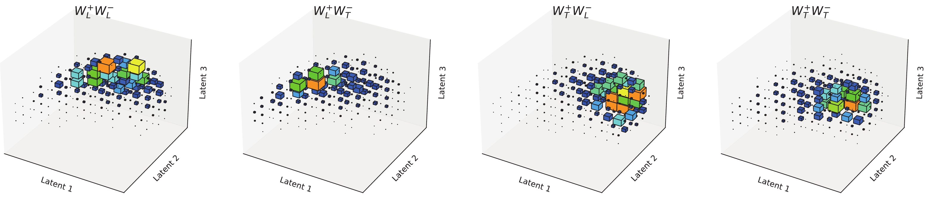
Figure 5. (color online) Normalized distributions of the latent features for different polarization modes in the semi-leptonic channel.
Two classes of variables that are used in the GBDT method to calculate the ROC curves are listed as follows:
● Detector-level variables: transverse momentum
$ p_T(\ell) $ and pseudorapidity$ \eta(\ell) $ of the lepton, azimuthal angle difference between the forward-backward jets$ \Delta \phi (j,j) $ and the transverse momentum of the W boson pair$ p_T(W,W) $ which can be calculated by vector-summing the transverse momenta of its decay products (including the missing transverse momentum).● Truth-level variables: transverse momenta of two W bosons
$ p_T(W^\pm) $ , the lepton angle in the W boson rest frame$ \cos(\ell) $ , and the invariant mass$ m_{jj} $ of the forward-backward jets.The ROC curves for methods under different inputs are presented in the left-hand panel of Fig. 6. Even though the semi-leptonic channel only contains one neutrino in the final state, the large uncertainty in jet measurement and the similarities between forward-backward and W-boson-decay-generated jets render the polarization-discriminating power of this channel similar to that of the dileptonic one. However, owing to the sizable production rate of this channel, a dataset with an integrated luminosity of
$ \lesssim 600 $ fb$ ^{-1} $ can be used to probe the 1% change in the$ W^+_L W^-_L jj $ fraction.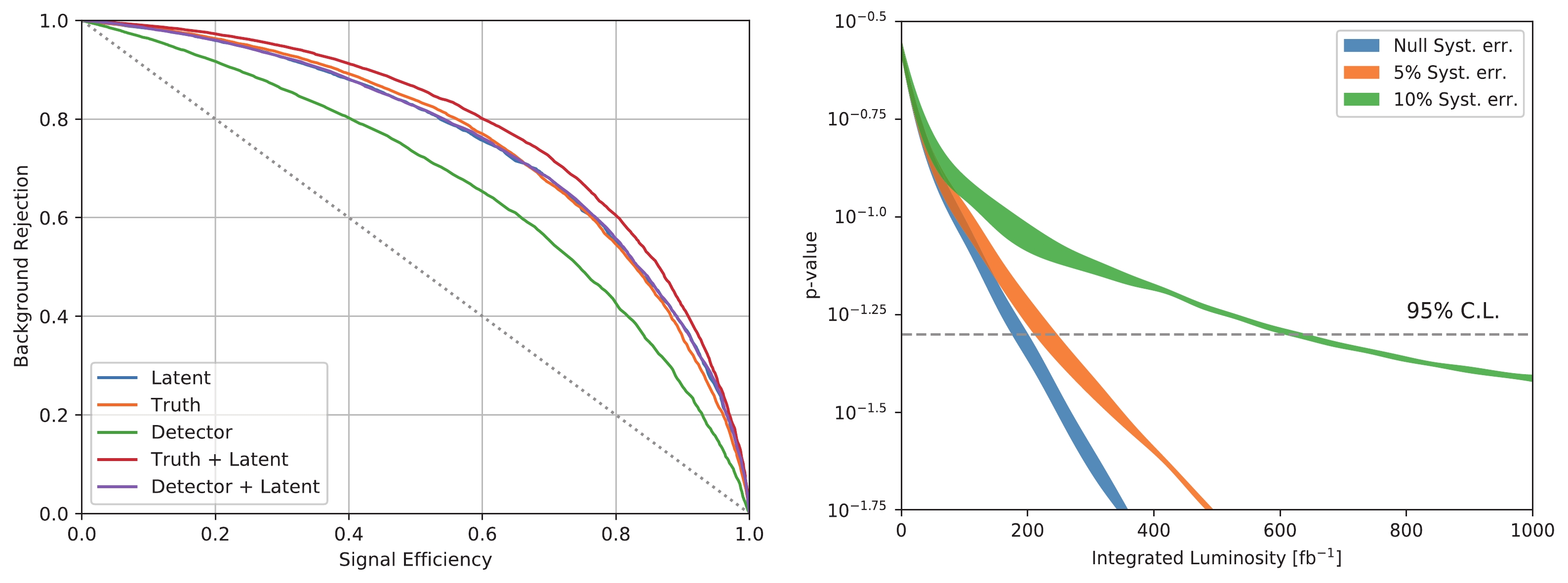
Figure 6. (color online) Same as Fig. 4 but for the semi-leptonic channel. Note that the variables used for plotting the ROC differ from those in the dileptonic channel.
It should be noted that this result is only provided as a rough estimation. In a concrete model, the differential cross-section of the EW
$ W^+ W^- j j $ channel cannot be simply given by the combination of the SM polarization components. Variables other than those listed above can help to discriminate different polarizations. Meanwhile, the contribution from the SM background processes should be taken into account. In the following two sections, we consider the EFT and 2DHM as a case study. -
In the absence of direct observations of new states, an EFT-based description (valid up to the scale of new physics) represents a practical method for investigating new physics. The EFT contains a complete set of independent gauge-invariant operators composed of the SM fields. Numerous studies have sought to constrain the coefficients of these operators with precise experiments [51-55]. Most operators are tightly constrained by the electroweak precision tests (EWPT) of the SM. We consider the operator [56, 57]
$ \mathcal{O}_H = \frac{\bar{c}_H}{2 v^2} \partial^\mu [\Phi^\dagger \Phi] \partial_\mu [\Phi^\dagger \Phi] \Rightarrow \frac{\bar{c}_H}{2} \partial^\mu h \partial_\mu h $

(6) because it is less constrained by the EWPT. The
$ \Phi $ field is a Higgs doublet and h denotes the Higgs boson field with the vacuum expectation value$ v = 246.2 $ GeV. The$ \mathcal{O}_H $ operator contributes to the Higgs boson kinetic term, and the field redefinition required to return the kinetic term to its canonical form is as follows:$ h \to h \left[1 - \frac{1}{2} c_H\right]. $

(7) This leads to the following changes to the Higgs couplings:
$ \begin{aligned}[b] \mathcal{L}_{H} \supset & \frac{g m_W}{c^2_W} \left[1- \frac{1}{2} \bar{c}_H \right] Z_\mu Z^\mu h + g m_W \left[1-\frac{1}{2}\bar{c}_H \right] W^\dagger_\mu W^\mu h \\ &+ \left[ \frac{y_f}{\sqrt{2}} \left[1-\frac{1}{2}\bar{c}_H\right] \bar{f} P_R f h +{\rm h.c.}\right]\; . \end{aligned} $

(8) The updated global fit to the EFT coefficients constrains
$ \bar{c}_H \lesssim 0.4 $ (neglecting all other operators) [58]. Future lepton colliders (e.g., the ILC) will constrain the$ \bar{c}_H $ to the 1% level [59].We study the effects of this on EW
$ W^+ W^- jj $ production at the LHC. The polarization vector$ \epsilon_L^\mu \sim \dfrac{p^\mu}{m_V} + \mathcal{O}\left(\dfrac{m_V}{E}\right) $ increases with momentum p; hence, the longitudinally polarized gauge boson scattering ($ W_L W_L \to W_L W_L $ ) dominates at high energies. In the high-energy limit, the amplitude for longitudinal W boson scattering (without Higgs contribution) is$ \mathcal{M}^{\rm{gauge}} = -\frac{g^2_w}{4 m^2_W} u + \mathcal{O}(s^0)\; , $

(9) which cancels with the amplitude from the Higgs exchange
$ \mathcal{M}^{\rm{Higgs}} = - \frac{g^2_w}{4 m^2_W} \left[\frac{(s-m^2_W)^2}{s-m^2_H} + \frac{(t-m^2_W)^2}{t-m^2_H}\right] \stackrel{s,t,u \gg m_W, m_H}{\sim} \frac{g^2_w}{4 m^2_W} u\; , $

(10) leaving terms that do not increase with energy. Here,
$ s,t,u $ are Mandelstam variables. However, the cancellation only holds if the Higgs boson's couplings to gauge bosons are exactly SM-like. The$ \mathcal{O}_H $ operator modifies the Higgs boson couplings as shown in Eq. (8), leading to an incomplete cancellation up to the scale at which new physical states emerge. As a result, the fraction of$ W^+_L W^-_L jj $ is increased and the kinematic properties of the final states are changed.We adopt the Universal FeynRules Output (UFO) model (as implemented in Ref. [60]) to generate the EW
$ W^+ W^- j j $ events in the EFT. All coefficients except$ \bar{c}_H $ are set to zero. Both the di- and semi-leptonic channels are considered. Only those events that pass through the preselection cuts (as listed in Sec. IIA) are fed into the network for further analyses. The production cross-section of the EW$ W^+ W^- j j $ process (for different choices of$ \bar{c}_H $ ) before and after preselections are given in Table 2. The$ \bar{c}_H = 0 $ case corresponds to the SM. We find that the fraction of the longitudinal W production increases with$ |\bar{c}_H| $ as the cancellation become less exact. Furthermore, our preselection cuts can increase the fraction of the longitudinal$ W^+_L W^-_L j j $ , especially for the dileptonic channel. After the preselections, the production rate of the semi-leptonic channel is one order of magnitude larger than that of the dileptonic one.$ \bar{c}_H $ 

$\sigma^0_{m_{jj} > 500} {\rm{ /fb} }$ 

$\sigma_{ll} {\rm{ /fb} }$ 

$\sigma_{lj} {\rm{ /fb} }$ 

$\sigma^{LL}_{m_{jj} > 500} {\rm{ /fb} }$ 

$\sigma^{LL}_{ll}{\rm{ /fb} }$ 

$\sigma^{LL}_{lj}{\rm{ /fb} }$ 

−1.0 440.6 4.82 40.2 46.29 0.754 5.28 −0.5 421.8 4.44 37.7 29.68 0.397 3.04 0 419.7 4.36 37.3 25.84 0.314 2.40 0.5 426.7 4.48 37.9 28.79 0.356 2.79 1.0 436.2 4.62 39.3 34.01 0.462 3.50 Table 2.
$ \sigma^0_{m_{jj}>500} $ and$ \sigma^{LL}_{m_{jj}>500} $ are the production cross-sections (requiring the invariant mass of forward-backward jets to exceed 500 GeV at parton level) for the total and longitudinally polarized EW$ W^+ W^- jj $ productions.$ \sigma^{(LL)}_{ll/lj} $ corresponds to the cross-section of the dileptonic channel ($ ll $ ) and semi-leptonic channel ($ lj $ ) after preselection cuts.In this and the following section, the same network (trained on the labeled SM background processes and the SM
$ W^{\pm}W^{\mp}jj $ for different polarizations) is used for testing. Events of the new physics are not used for training the network, to demonstrate that our method is model-agnostic. Analyzing the preselected events of both SM background processes and the EFT processes for the pre-trained network, we can obtain the distributions of those processes in the three-dimensional latent space. The normalized distributions are presented in Fig. 7, where the background corresponds to the weighted sum of all SM processes (including$ t t_\ell $ ,$ t W_\ell $ /$ t_\ell W $ ,$ W_\ell W j j^{\rm{QCD}} $ ,$ W_\ell Z j j^{\rm{QCD}} $ , and$ W_\ell Z j j^{\rm{EW}} $ ) as discussed in Sec. IIA. Because the network is trained to classify the SM background processes using the SM$ W Wj j^{\rm{EW}} $ , the background events are well separated from the signal events (EW$ W Wj j $ production in the EFT), as predicted. Moreover, the distributions of EW$ W Wj j $ production under different values of$ \bar{c}_H $ visibly differ. This feature can be used to constrain the value of$ \bar{c}_H $ .
Figure 7. (color online) Normalized distributions of latent features for different processes in the di- (upper panels) and semi- (lower panels) leptonic channels. Processes (from left- to right-hand panels) correspond to the backgrounds and EW
$ W^+ W^- jj $ productions in the EFT model with$ \bar{c}_H = -1.0,\; 0,\; 1.0 $ , respectively.To measure the consistency of the SM and EFT for non-zero
$ \bar{c}_H $ , we perform a binned log-likelihood test in the latent space. As discussed in Sec. IIC, the ten bins with the highest signal-to-background ratios are used. According to our simulation, this includes$ \sim $ 30% signal events and$ \sim $ 0.5% background events after preselection. The null hypothesis is the SM backgrounds + SM EW$ W^+W^- j j $ , and the test hypothesis is the SM backgrounds + EFT EW$ W^+W^- j j $ with a non-zero$ \bar{c}_H $ . The integrated luminosity required to achieve a 95% confidence level (CL) probing for different$ \bar{c}_H $ are presented in Fig. 8. It can be seen that the semi-leptonic channel outperforms the dileptonic one if the systematic uncertainty can be controlled below$ \sim $ 5%. Owing to the higher backgrounds in the semi-leptonic channel, the sensitivity drops rapidly when the systematic uncertainty exceeds 5%. With a systematic uncertainty of ~5%, our method can constrain the$ \bar{c}_H $ to [-0.2,0.1] in high-luminosity LHC conditions.
Figure 8. (color online) Integrated luminosity required to probe the signal (for different
$ \bar{c}_H $ ) at 95% CL in the di- (left panel) and semi- (right panel) leptonic channels. Several different systematic uncertainties are considered. -
Because our network is trained to detect anomalies in the simulated SM processes, it could be sensitive to the errors in the simulation. In Fig. 9, we show how the results of our shape analyses vary when the testing samples are simulated independently from the training ones. To calculate the p-values in the figure, the null hypothesis is always the SM prediction with events simulations, as discussed above. In the test hypothesis (NSM and N
$ \bar{c}_H $ ), the events of the SM processes are simulated independently with Herwig++ [61, 62] for parton showers and hadronization, and Delphes (with ATLAS parameters) for detector simulation. For the SM processes, two independent simulations produce 5% (3%) systematical deviations in the selected bins for the dileptonic (semileptonic) channel. As a result, if the systematic uncertainty in the shape analysis is chosen to be smaller than the systematical deviations caused by the simulation, the event samples of two simulations for the SM processes can be distinguished, as shown by the blues lines in both panels. Moreover, the difference between the simulations in the null and test hypotheses produces an over-optimistic sensitivity to new physics, although the effect is moderate when the systematic uncertainty in the shape analysis is chosen to be large.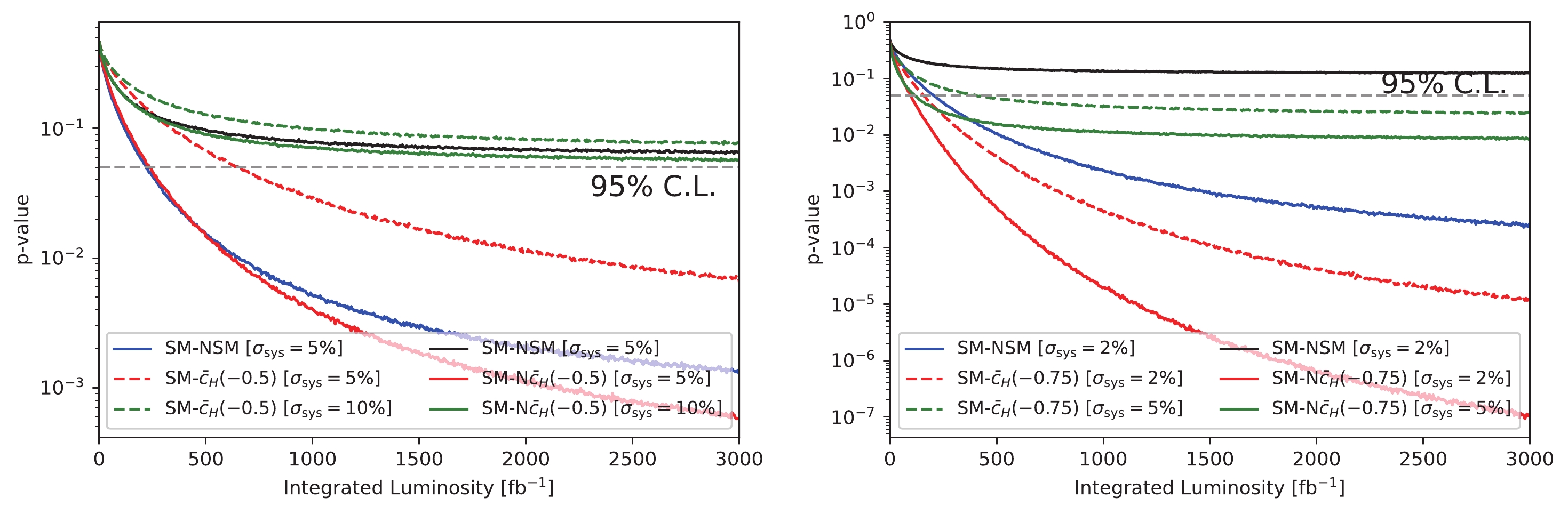
Figure 9. (color online) The p-values (at varying integrated luminosity) for independent simulations of event samples and benchmark points. Left panel: dileptonic channel with benchmark point
$ \bar{c}_H = -0.5 $ . Right panel: semileptonic channel with benchmark point$ \bar{c}_H = -0.75 $ . SM denotes the null hypothesis with events simulated as described above. For NSM and N$ \bar{c}_H $ , the background events are simulated using Herwig++. The$ \sigma_{\text{sys}} $ denotes the systematic uncertainty that we adopt in the binned log-likelihood analysis. -
The EFT description may not be valid when the collision energy approaches the masses of the new states. Here, we consider a complete ultraviolet model, the 2HDM [63, 64], which is one of the simplest Higgs sector extensions of the SM. The scalar sector of the 2HDM consists of two
$ SU_{W}(2) $ doublets. A discrete$ Z_2 $ symmetry is imposed to prevent tree-level flavor-changing neutral currents. Depending on how this symmetry is extended to the fermion sector, four versions of the 2HDM can be realized. The type-II case is considered in this work. The 2HDM predicts numerous remarkable signatures at hadron colliders. In particular, resonant signals are predicted, owing to the existence of extra CP-even, CP-odd, and charged scalars. Instead of performing a dedicated search for each of these signals, we show that our method is sensitive to changes in the polarization and kinematic properties of EW$ W^+ W^- j j $ production in the 2HDM. Comparing the latent features of the$ W^+ W^- j j $ process in the 2HDM with their measured values, constraints on the parameters of the 2HDM can be obtained.The type-II 2HDM contains six parameters: the scalar masses (
$ m_{H_1}, m_{H_2} $ ,$ m_A $ , and$ m_{H^\pm} $ ), the mixing angle$ \alpha $ between two CP -even scalars, and the ratio$ \tan \beta $ . The$ m_{H_1} $ has been measured to be ~125 GeV. The$ m_A $ and$ m_{H^\pm} $ are irrelevant in the$ W^+ W^- j j $ production; their masses are set to 3 TeV to prevent decays of$ H_2 $ into those states. The couplings of CP-even scalars to W bosons are given by$ \mathcal{L} \supset \frac{2 m^2_W}{v} \sin (\alpha-\beta) H_1 W^+_{\mu} W^{\mu -} + \frac{2 m^2_W}{v} \cos (\alpha-\beta) H_2 W^+_{\mu} W^{\mu -}\; . $

(11) Thus, the combination
$ \sin (\alpha-\beta) $ is often used to replace the$ \alpha $ parameter. The$ \tan \beta $ is not related to the$ HWW $ couplings; however, it can modify the scalar couplings to fermion ones, which affects the total decay width of the$ H_2 $ and therefore the kinematics of$ W^+ W^- jj $ . We choose$ \tan \beta = 5 $ for simplicity⑦. Hence, we are left with two free parameters:$ m_{H_2} $ and$ \sin (\alpha-\beta) $ . The partial widths of$ H_2 $ are given by$ \Gamma(H_2 \to WW) = \frac{g_w^4 \cos^2(\alpha-\beta) v^2 }{256 \pi m_{H_2}} \sqrt{1- 4 \frac{m_W^2}{m^2_{H_2}}} \frac{m_{H_2}^4 - 4 m_{H_2}^2 m^2_W +12 m^4_W }{m^4_W} \; , $ 
(12) $ \Gamma(H_2 \to ZZ) = \frac{(g')^4 \cos^2(\alpha-\beta) v^2}{512 \pi m_{H_2}} \sqrt{1-4 \frac{m^2_Z}{m^2_{H_2}}} \frac{m_{H_2}^4-4m_{H_2}^2 m_Z^2 +12 m^4_Z}{m^4_Z} \; , $

(13) $ \Gamma(H_2 \to t\bar{t}) = \frac{3 y_t^2 (\sin(\beta - \alpha)- \tan \beta \cos(\beta-\alpha))^2}{16 \pi m_{H_2} \tan^2 \beta} \sqrt{1-\frac{4 m_t^2}{m^2_{H_2}}} (m^2_{H_2} - 4 m^2_t) \; , $

(14) $ \Gamma(H_2 \to b\bar{b}) = \frac{3 y_b^2 (\cos(\beta - \alpha)- \tan \beta \sin(\beta-\alpha))^2}{16 \pi m_{H_2} } \sqrt{1-\frac{4 m_b^2}{m^2_{H_2}}} (m^2_{H_2} - 4 m^2_b) \; , $

(15) with
$ g' = \cos(\theta_w) g_w + \sin(\theta_w) g_1 $ , and$ y_t $ /$ y_b $ represents the Yukawa coupling of the top/bottom quark.The model is implemented in FEYNRULES [65]; this generates the UFO model files for the MG5, to calculate the leading-order production cross-section and simulate the events. As an illustration, in Table 3, we present the production cross-sections of the EW
$ W^+ W^- jj $ process for several points in the 2HDM. In particular, the contribution of the heavy scalar$ H_2 $ is taken into account, which generally increases the total production rate⑧.$ (m_{h_2}, \sin(\beta - \alpha)) $ 

$\sigma^0_{m_{jj} > 500}{\rm{ /fb} }$ 

$\sigma_{ll} {\rm{ /fb} }$ 

$\sigma_{lj} {\rm{ /fb} }$ 

$\sigma^{LL}_{m_{jj} > 500} {\rm{ /fb} }$ 

$\sigma^{LL}_{ll} {\rm{ /fb} }$ 

$\sigma^{LL}_{lj} {\rm{ /fb} }$ 

(300, 0.7) 636.2 8.362 64.07 170.75 2.91 20.78 (300, 0.9) 492.5 5.853 46.52 79.81 1.27 9.35 (700, 0.7) 461.9 5.527 43.70 71.58 1.30 9.50 (700, 0.9) 428.5 4.842 39.33 42.65 0.676 5.06 Table 3. Similar to Table 2 but for the 2HDM model. The corresponding parameters are given in the first column.
The cancellation between the amplitudes with and without Higgs exchange are delayed to the scale of
$ m_{H_2} $ , and the heavy scalar predominantly decays into a longitudinally polarized vector boson; hence, the fraction of$ W^+_L W^-_L jj $ is considerably larger than that of the SM. For relatively light$ H_2 $ and small$ \sin(\beta-\alpha) $ (which implies the significant contribution of$ H_2 $ ), the fraction of$ W^+_L W^-_L jj $ can reach$ \sim $ 30% before preselection cuts are applied, whereas it reaches 6% in the SM. The preselections can increase the fraction even further. This renders our network very sensitive to the signals in the 2HDM.Moreover, the existence of the
$ H_2 $ resonance in$ W^+W^- jj $ production also generates discriminative features in the final state. In Fig. 10, we plot the normalized distributions of latent features for the$ W^+W^- jj $ production from pure$ H_2 $ resonances in the dileptonic channel. Different masses of the$ H_2 $ exhibit distinct distributions in the latent space; thus, the network is not only capable of classifying the polarizations of the vector bosons but is also sensitive to their kinematic properties, even though those 2HDM events are not used for trainning.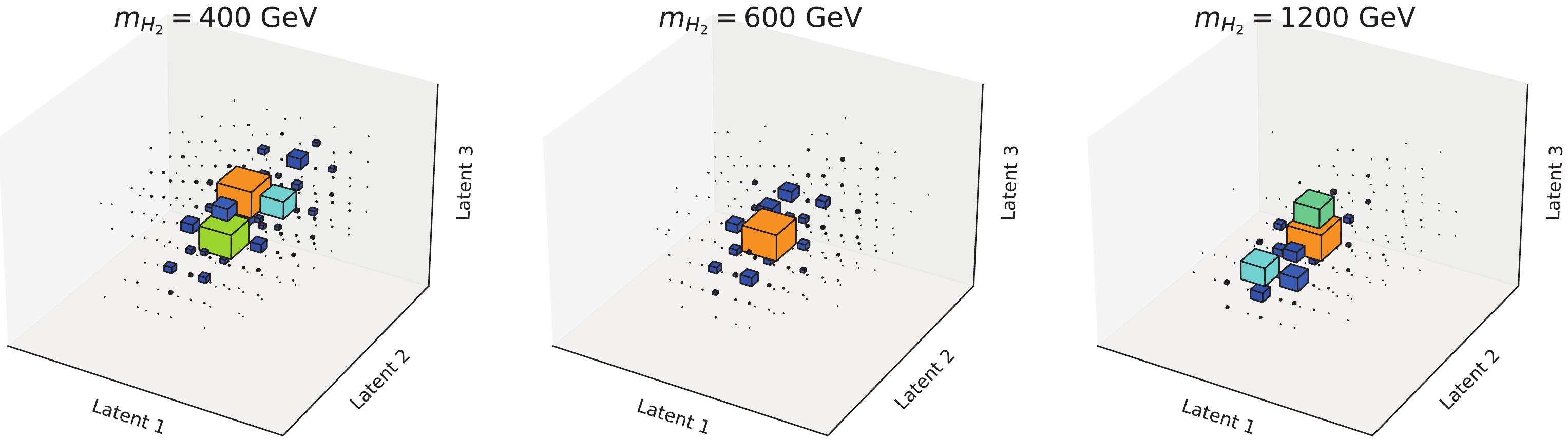
Figure 10. (color online) Normalized distributions of the latent features for the resonant
$ H_2 $ production and decay$ H_2 \to W^+ W^- $ in the dileptonic channel. The mass of the$ H_2 $ is given in the title of each subfigure.Finally, we input the preselected events in the di- and semi-leptonic channels to the pre-trained network, to extract the latent features. The binned log-likelihood test is performed in the latent space, to identify the discovery potential of models with different parameters in 2HDM. Similar to before, the null hypothesis is taken as the SM background + SM EW
$ W^+ W^- j j $ , and the test hypothesis is taken as the SM backgrounds (assuming these processes are left intact in 2HDM) + EW$ W^+ W^- j j $ in 2HDM for different sets of parameters. The integrated luminosity required to achieve a 95% CL probing on the$ m_{H_2} $ -$ \sin(\beta-\alpha) $ plane is shown in Fig. 11 for the di- and semi-leptonic channels, respectively. In contrast, in the traditional heavy Higgs resonant searches [66, 67], the sensitivities drop quickly at large$ m_{H_2} $ , owing to the suppressed production rate. Our method probes both the resonant features and the modifications to the Higgs couplings, simultaneously. The parameter space featuring a$ H_2 $ as heavy as 1.5 TeV can be probed with a relatively low integrated luminosity, provided the$ \sin(\beta-\alpha) $ is not too close to one. However, when$ \sin(\beta-\alpha) \to 1 $ (the alignment limit), our method loses all sensitivity. Searches for the resonances in fermionic channels are still able to constrain the model [68-71], because their productions are mainly controlled by the Yukawa couplings. The production cross-sections of both channels (before the preselection cuts) are indicated by the color grades in the figure. The sensitivity of the method is roughly determined by the cross-section, even though a slightly better sensitivity can be achieved in the small$ \sin(\beta - \alpha) $ region (e.g., compared to the the point [$ m_{H_2} = 300\; \text{GeV}, \sin (\beta -\alpha) = 0.9 $ ], a lower integrated luminosity is required to probe the point [$ m_{H_2} = 550\; \text{GeV}, \sin (\beta -\alpha) = 0.7 $ ], despite their similar production cross-sections). The improvement of the sensitivity is attributed to the fact that the point with a smaller$ \sin (\beta -\alpha) = 0.7 $ contains a larger fraction of the longitudinal W boson.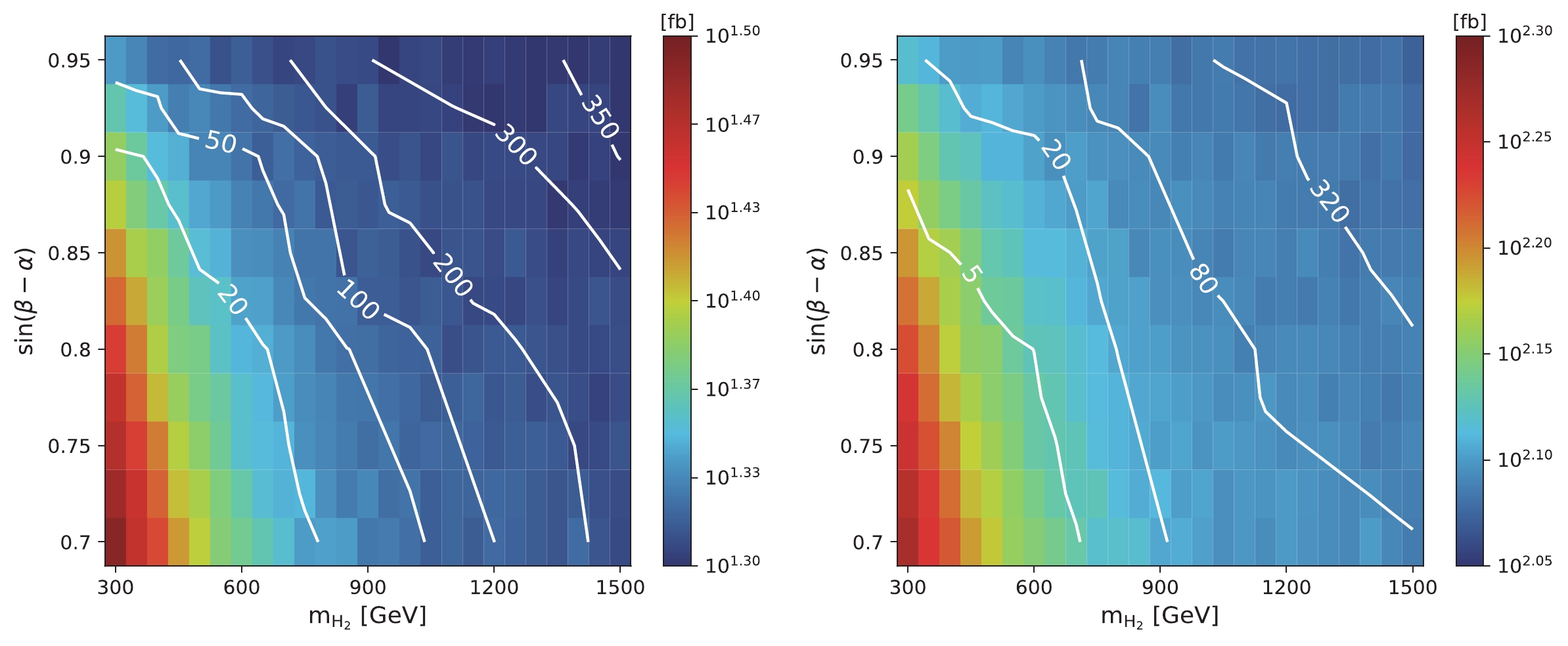
Figure 11. (color online) Contours corresponding to the integrated luminosity required to probe the signal [for different
$ \sin(\beta - \alpha) $ and$ m_{H_2} $ ] at a 95% CL. The color grades correspond to the fiducial cross-sections (requiring$ m_{jj} >500 $ GeV at parton level) multiplied by the branching ratios. The systematic uncertainties are set to 5% for both the di- (left) and semi- (right) leptonic channels. -
In this work, we constructed a neural network that consisted of a classification network and an autoencoder. When inputted with low-level information (here, the 4-momenta and the identities of particles), the network could reduce the dimensionality of the feature space for
$ WWjj $ production, without an excessive loss of discriminative power (i.e., to discriminate the EW$ WWjj $ from other processes and discriminate between the different polarization modes of the EW$ WWjj $ ). We found that the feature space of both the di- and semi-leptonic channels could be compacted into three dimensions. By performing a binned log-likelihood test on the distributions of latent features, we could determine whether the data were consistent with the SM predictions. We showed that these latent features were highly sensitive to various possible new physics contributing to the VBS. Although the scores given by the classifier network contained a certain amount of the process information, they were not as complete as the latent features. In Fig. 12, we present the sensitivities of the latent features and the sensitivities of the scores⑨ obtained by the classifier for two benchmark points in the EFT and 2HDM. As predicted, the latent features facilitated superior sensitivities. In particular, the remarkable kinematic features of the 2HDM were not very useful for classifying SM processes; thus, this sort of information might be lost in the scores given by the classifier. Compared to the EFT case, the advantages of using latent features were much more significant in the 2HDM model.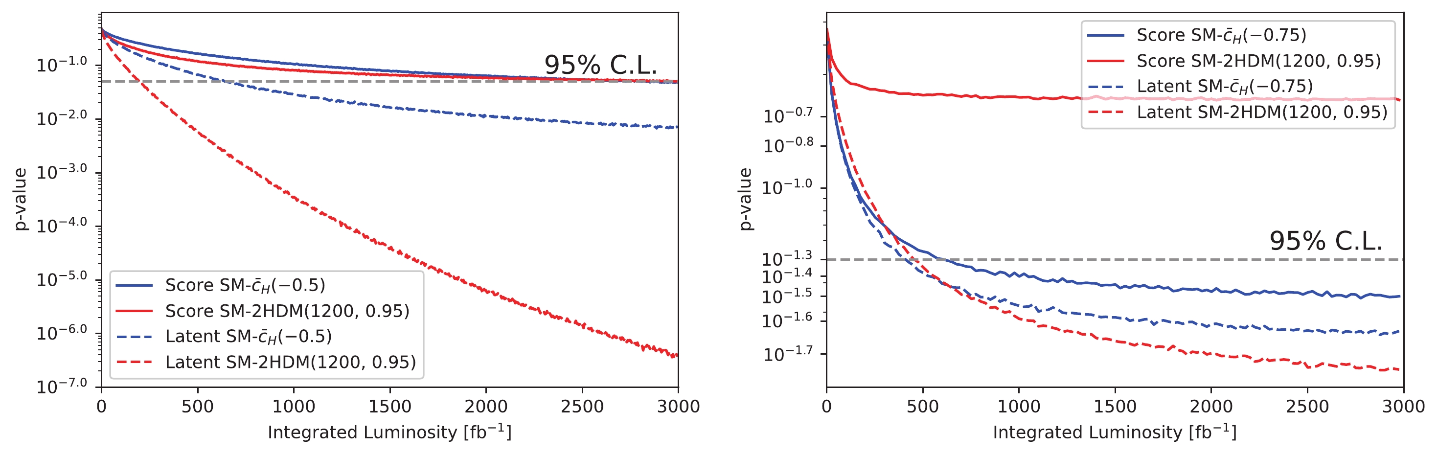
Figure 12. (color online) The p-value (at varying integrated luminosities) of the shape analysis in latent space (dashed lines) and the p-value calculated only using the classifier score (solid lines) for di- (left-hand panel) and semi- (right-hand panel) leptonic channels.
By considering both the di- and semi-leptonic channels of
$ W^+W^- jj $ production, we showed that our network can efficiently classify different polarization modes. When neglecting the background, the LHC dataset with integrated luminosity$ \lesssim 600 $ fb$ ^{-1} $ was sufficient to probe the 1% change in the longitudinal$ W^+W^- j j $ fraction, using the semi-leptonic channel. The dileptonic channel was less sensitive, owing to its low production rate. Then, the network was applied to the EFT with a non-zero$ \mathcal{O}_H $ operator and the type-II 2HDM; the background effects were included, to obtain more complete and realistic results. In the EFT, our method could constrain the coefficient$ \bar{c}_H $ to [-0.2,0.1], provided that the systematic uncertainty was ~5%. The dileptonic channel outperformed the semi-leptonic channel when the systematic uncertainty exceeded 5%. In the 2HDM, because our method was sensitive to both the resonant decay$ H_2 \to W^+ W^- $ and the SM Higgs coupling modifications, the entire region with$ \sin(\beta - \alpha) \lesssim 0.95 $ and$ m_{H_2} \lesssim 1.5 $ TeV can be probed with a integrated luminosity of$ \sim $ 300 fb$ ^{-1} $ at the LHC.We note that modifications of the SM are unlikely to be confined to VBS processes. By assuming a new physics scenario of some kind, model-dependent searches can be more effective at identifying signals. Our method may not be as sensitive as these more specific searches. For example, in the 2HDM with
$ \tan\beta = 5 $ , our method is insensitive to the parameter space in which$ \cos(\beta - \alpha) = 0.05 $ [corresponding to$ \sin(\beta - \alpha) = 0.9987 $ ]. On the other hand, searches for$ H\to \tau \tau $ at the LHC have already excluded the parameter space with$ m_{H} \sim [200,350] $ GeV [68-70]. The advantage of our method is that it is suitable for detecting a wide range of new physics contributing to the VBS (i.e., relevant to SM ESB). This is especially useful when the forms of the new physics are unknown.
Detecting anomalies in vector boson scattering
- Received Date: 2020-12-07
- Available Online: 2021-07-15
Abstract: Measuring vector boson scattering (VBS) precisely is an important step toward understanding the electroweak symmetry breaking of and detecting new physics beyond the standard model (SM). Herein, we propose a neural network that compresses the features of the VBS data into a three-dimensional latent space. The consistency of the SM predictions and experimental data is tested via binned log-likelihood analysis in the latent space. We show that the network is capable of distinguishing different polarization modes of WWjj production in both di- and semi-leptonic channels. The method is also applied to constrain the effective field theory and two Higgs Doublet Model. The results demonstrate that the method is sensitive to general new physics contributing to the VBS.


 DownLoad: