


 Abstract
 HTML
HTML Reference
 Related
 PDF
PDF


-
With the development of theory, researchers found a fundamental relationship between gravity, thermodynamics and quantum theory. Initially, physicists studied the mechanics of black holes [1], and then, they found that if they applied quantum field theory in curved spacetime to the fundamental properties of black holes, they could obtain profound results. The framework of black hole thermodynamics is based on the discovery made by Bekenstein and Hawking that black holes have entropy and other thermodynamic quantities [2-5]. The Schwarzschild black hole in AdS space was investigated by Hawking and Page [6], where the phase transition from thermal AdS to a black hole was found. A black hole has negative specific heat in asymptotically flat spacetime, which causes it to be an unstable system. The problem in asymptotically flat space can then be avoided, as the gravitational potential of AdS space acts as a box of finite volume with unphysical perfectly reflecting walls [6]. In addition, the emergence of AdS/CFT correspondence [7-9] has also inspired relevant studies on black hole thermodynamics [10-17].
Another preferred solution to solve this problem is to surround the black hole with a cavity. The Dirichlet boundary condition is supposed to be considered in the wall of the cavity. This work was first carried out by York [18], in which the Hawking-Page-like phase transition was found. Subsequently, it was extended to the case of an RN black hole, which was considered in a grand canonical ensemble [19] and a canonical ensemble [20, 21]. The thermodynamic phases of diverse black holes in a cavity were discussed in [22-31], which indicated that the van der Waals-like phase transitions or Hawking-Page-like phase transitions exist invariably except for some particular cases. The relationship between the thermodynamic properties of black holes and their specific boundary conditions in different extended phase spaces was studied in [32]. Apart from this, other systems such as charged scalars, boson stars, and hairy black holes in a cavity were investigated in [33-36], which concluded that there are some surprising similarities between gravity systems in a cavity and holographic superconductors in AdS gravity. The stabilities of solitons, stars, and black holes in a cavity were also discussed in [37-44]. Recently, McGough, Mezei, and Verlinde proposed that in the holographic dual, the
$ T\bar{T} $ deformed CFT$ _{2} $ is located on a Dirichlet wall at a finite radial distance of AdS$ _3 $ in the bulk [45], which also inspires us to study the properties of black holes in a cavity.From observations, we know that the universe is dominated by an energy component with an effective negative pressure [46, 47]. One hypothesis for such a component is the cosmological constant, and other hypotheses are dynamical vacuum energy or quintessence [48-53]. Quintessence is described by an ordinary scalar field minimally coupled to gravity, with particular potentials that lead to late time inflation. The quintessence field must couple to ordinary matter and will lead to long range forces and time dependence of the constants of nature when it is suppressed by the Planck scale. The static spherically symmetric solution with the quintessential matter surrounding a charged black hole was first presented in [54]. Since then, a series of studies about black holes in the presence of quintessence have been conducted. Quintessence modes were studied in [55, 56], and thermodynamics including Hawking radiation, heat engines, and phase transition in the holographic framework were investigated in [57-66]. In particular, the phase transition of the quintessence RN-dS black hole was studied through the effective thermodynamic quantities [67]. Although many relevant works have been completed, there is no research that combines quintessential matter and cavity boundary condition. In addition, the discovery about the difference in phase structures of black holes between AdS space and a Dirichlet cavity [28-31] also prompts us to investigate the phase structures of black holes from another perspective.
In this paper, we study the phase structures and transitions of RN black holes surrounded by quintessence dark energy under two different boundary conditions, i.e., AdS space and a Dirichlet wall. Moreover, a grand canonical ensemble is considered, which indicates that the temperature and potential of the black hole are fixed on AdS boundary condition, while the temperature and potential of the cavity wall are fixed on Dirichlet wall boundary condition. The paper is organized as follows. In Sec. II, we discuss the phase structures and transitions of an RN-AdS black hole surrounded by quintessence dark energy. In Sec. III, we study the phase structures and transitions of RN black holes surrounded by quintessence dark energy in a cavity. The final summaries and discussions are presented in Sec. IV.
-
In this section, we discuss the phase structures and transitions of the RN black hole surrounded by quintessence dark energy in AdS space. The action of the black hole in four dimensional curved space-time is [68]
$ {\cal{S}} = \frac{1}{16\pi}\int {\rm d}^4 x(\sqrt{-g}[R-2\Lambda-F^{\mu\nu}F_{\mu\nu}]+ {\cal{L}}_{q}). $

(1) In the above action, the cosmological constant
$ \Lambda = -3/l^2 $ , where l is the AdS space radius.$ {\cal{L}}_{q} $ is the Lagrangian of quintessence as a barotropic perfect fluid, which can be written as [69]$ {\cal{L}}_{q} = -\rho_q\left[1+\omega {\rm ln}\left(\frac{\rho_{q}}{\rho_0}\right)\right], $

(2) where
$ \rho_{q} $ is the energy density,$ \rho_{0} $ is an integral constant, and$ \omega $ is the barotropic index. The solution of the spherical symmetric charged quintessence RN-AdS black hole is given by$ {\rm d}s^2 = f(r){\rm d}t^2-\frac{{\rm d}r^2}{f(r)}-r^2({\rm d}\theta^2+{\rm sin}^2 \theta {\rm d}\phi^2), $

(3) and
$ f(r) = 1-\frac{2M}{r}+\frac{Q^2}{r^2}-\frac{a}{r^{3\omega+1}}+\frac{r^2}{l^2}, $

(4) where M and Q are the mass and charge of the black hole, respectively. The normalization factor a is related to the density of quintessence dark energy
$ \rho_{q} = -\frac{a}{2}\frac{3\omega}{r^{3(\omega+1)}}, $

(5) where a needs to be positive and the constraint on the barotropic index is
$ -1<\omega<-1/3 $ .As the horizon radius
$ r_h $ is the root of$ f(r_h) = 0 $ , we have$ M = \frac{r_{h}}{2}+\frac{Q^2}{2r_{h}}-\frac{a}{2r_{h}^{3\omega}}+\frac{r_{h}^3}{2l^2}. $

(6) In the discussion that follows, M is redundant so we replace it with
$ r_{h} $ . Thus, the Hawking temperature is given by$ T = \frac{f^{'}(r_{h})}{4\pi} = \frac{1}{4\pi r_{h}}\left(1+\frac{3r_{h}^2}{l^2}-\frac{Q^2}{r_{h}^2}+\frac{3a\omega}{r_{h}^{3\omega+1}}\right). $

(7) The potential and entrophy of the black hole are, respectively,
$ \Phi = \frac{Q}{r_h},\;\;\;\;\;\; S = \pi r_h^2. $

(8) In addition, free energy plays a crucial role in probing into the phase structures and transitions of a quintessence RN-AdS black hole in the grand canonical ensemble, and it is given by [30, 70]
$ F = M-TS-Q\Phi, $

(9) in which the mass of the black hole is interpreted as enthalpy [71]. Ignoring the variation of l, we express physical quantities in units of l from now on to simplify the subsequent calculation
$\begin{aligned}[b]& \widetilde{r}_{h} = r_h/l,\;\;\;\; \ \widetilde{a} = a/l^{3\omega+1},\;\;\;\; \ \widetilde{Q} = Q/l, \\ & \widetilde{T} = Tl,\;\;\;\;\ \widetilde{F} = F/l. \end{aligned} $

(10) The heat capacity at constant potential is
$ C_{\Phi} = T\left(\frac{\partial S}{\partial T}\right)_{\Phi} = 2\pi l^2 \widetilde{r}_{h} \widetilde{T} \left(\frac{\partial \widetilde{r}_{h}}{\partial \widetilde{T}}\right)_{\Phi}. $

(11) Thus, the sign of the heat capacity is the same as the sign of
$ \partial \widetilde{r}_h/\partial \widetilde{T} $ at constant potential. We eliminate Q by Eq. (7) and Eq. (8) to obtain$ \widetilde{T} = \widetilde{T}\left(\widetilde{r}_{h}, \Phi \right) $ $ \widetilde{T} = \frac{1}{4\pi \widetilde{r}_{h}}\left(1-\Phi^2+3\widetilde{r}_{h}^2+\frac{3\widetilde{a}\omega}{\widetilde{r}_{h}^{3\omega+1}}\right). $

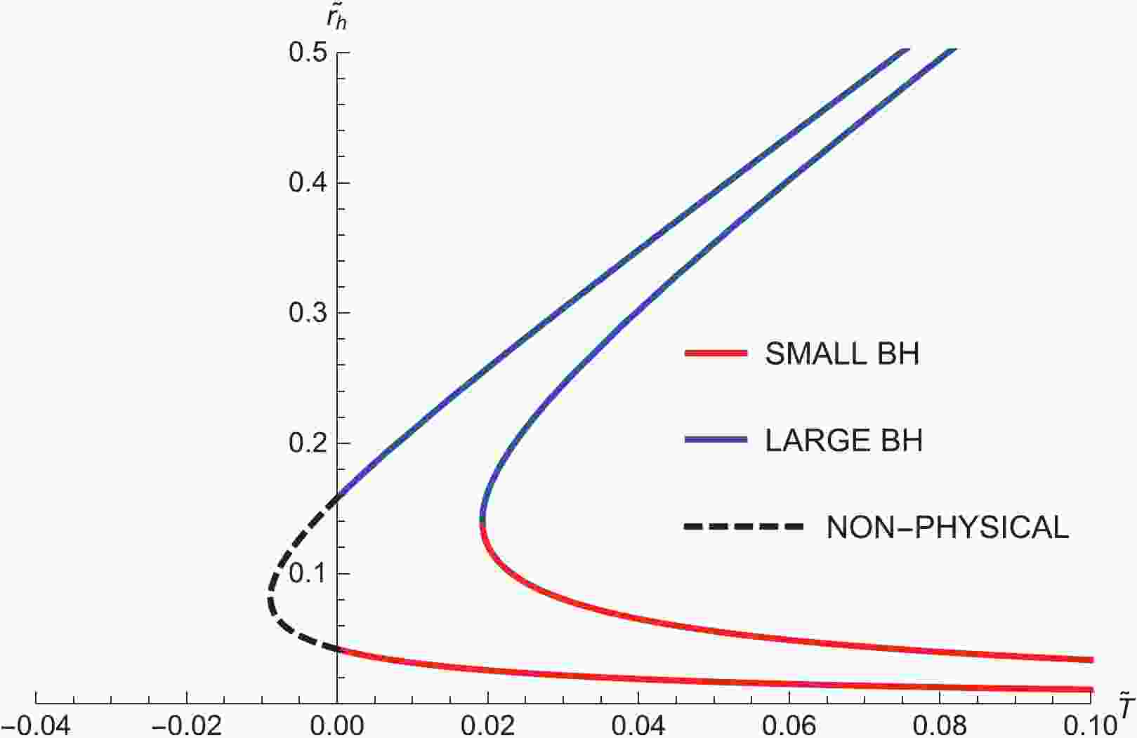
(12) According to Eq. (12), curves of the horizon radius
$ \widetilde{r}_{h} $ in terms of temperature$ \widetilde{T} $ with fixed values of$ \Phi $ are plotted in Fig. 1. For a fixed potential$ \Phi $ ,$ \widetilde{T}\left(\widetilde{r}_{h}, \Phi \right) $ has a minimum$ \widetilde{T}_{\rm min} $ . When$ \widetilde{T}>\widetilde{T}_{\rm min} $ , there are two branches, of which the Small BH with$ \partial\widetilde{r}_h/\partial\widetilde{T}<0 $ is thermodynamically unstable and the Large BH with$ \partial\widetilde{r}_h/\partial\widetilde{T}>0 $ is thermodynamically stable. There exists one section of non-physical curve in Fig. 1 because temperature cannot be negative.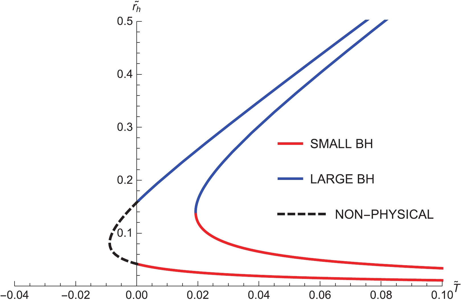
Figure 1. (color online) Plot of
$ \widetilde{r}_h $ against$ \widetilde{T} $ for different$ \Phi $ with$ \omega = -2/3 $ and$ \widetilde{a} = 0.3 $ , where$\Phi = 0.99, \; 0.97$ from left to right.It is worth noting that the thermal AdS space with a constant gauge potential is a classical solution of action (1) in the grand canonical ensemble, which should be also considered for our discussion. We find that there are two regions in
$ \Phi-\widetilde{a} $ phase space. As shown in Fig. 2, these two regions are referred to Region I and Region II. Specifically, in Region I, there exists a first-order phase transition as temperature$ \widetilde{T} $ increases. Nevertheless, in Region II, there is no phase transition.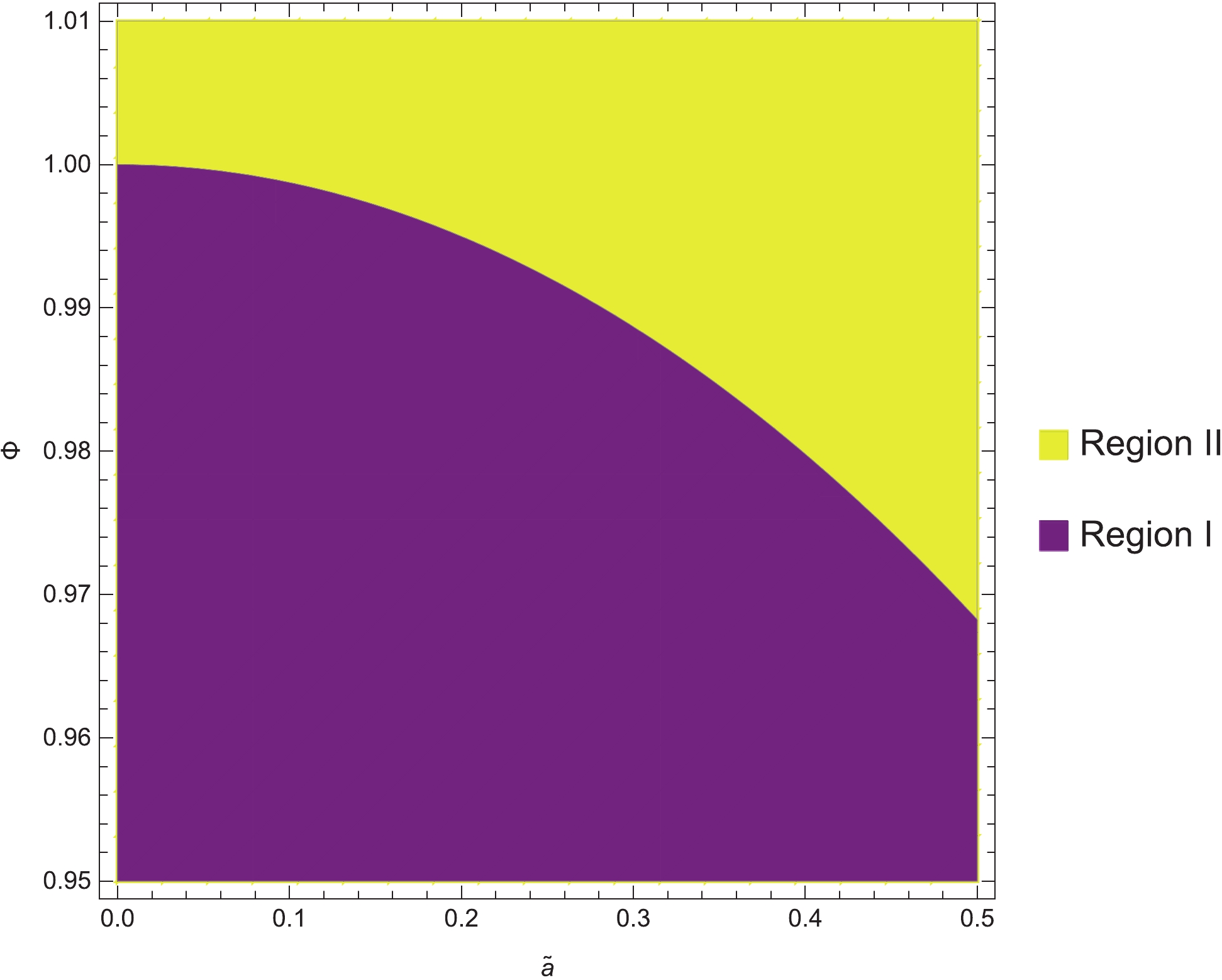
Figure 2. (color online) Two regions in
$ \Phi-\widetilde{a} $ phase space with$ \omega = -2/3 $ .We discuss the phase structures and transitions of the black hole in the abovementioned two regions. Our method is as follows. Eqs. (6) and (7) imply that M and T are functions of
$ r_{h} $ and Q. According to Eq. (8), the charge can be written as the function of$ r_{h} $ and$ \Phi $ , i.e.$ Q = Q(r_{h},\Phi) $ . Substituting it into$ M(r_{h},Q) $ and$ T(r_{h},Q) $ , we have$ M(r_{h},\Phi) $ and$ T(r_{h},\Phi) $ . Thus, F can be written as the function of$ r_{h} $ and$ \Phi $ according to Eq. (9). The quantity in units of l can be written as$ \widetilde{F}(\widetilde{r}_{h},\Phi) $ . The$ \widetilde{F}-\widetilde{T} $ diagrams with fixed$ \Phi $ are shown in Fig. 3 by regarding$ \widetilde{r}_{h} $ as the parameter. We notice that the behavior of the black hole for each value of$ \Phi $ is self-consistent with that shown in Fig. 1; that is, for$ \widetilde{T}>\widetilde{T}_{\rm min} $ , there are always two branches, i.e., Small BH and Large BH, which shows again that the Large BH is more stable than the Small BH because of the lower free energy. In Region I, when temperature$ \widetilde{T} $ increases from zero but does not exceed$ \widetilde{T}_{\rm min} $ , the thermal AdS is the only phase. When$ \widetilde{T}>\widetilde{T}_{\rm min} $ , the Small BH branch and Large BH branch appear, but the thermal AdS is still the globally stable state until the occurrence of a first-order phase transition. As$ \widetilde{T} $ increases further, the Large BH ultimately becomes the thermodynamically preferred state. This process is illustrated in Fig. 3(a). In Region II, there is no phase transition. Apparently, for any given temperature, Large BH is always the globally stable phase, as shown in Fig. 3(b).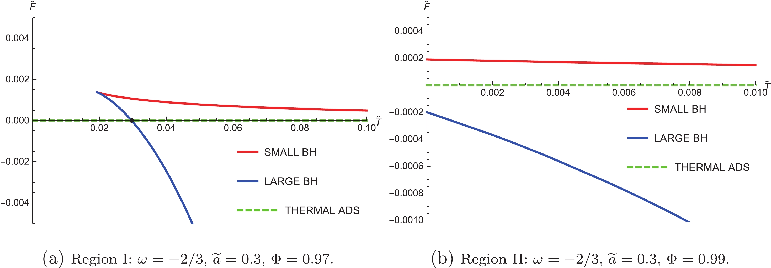
Figure 3. (color online) Plots of free energy
$ \widetilde{F} $ against temperature$ \widetilde{T} $ for fixed$ \Phi $ of two regions. The black dot is where a first-order phase transition occurs.Another
$ \widetilde{T}-\Phi $ phase diagram is displayed in Fig. 4. To avoid misunderstandings, the Small BH and Large BH are both denoted as Black Hole. We keep the parameters fixed; that is, we set$ \omega = -2/3 $ and$ \widetilde{a} = 0.3 $ in Fig. 4(a). The temperature of the phase transition decreases to zero as$ \Phi $ rises. Another homologous phase diagram is shown in Fig. 4(b), in which we adjust$ \omega = -2/5, -2/3, -9/10 $ , respectively, and$ \widetilde{a} = 1 $ . Compared with the former, this case is slightly distinct but the similarity is that there is only a first-order phase transition from the thermal AdS to Black Hole.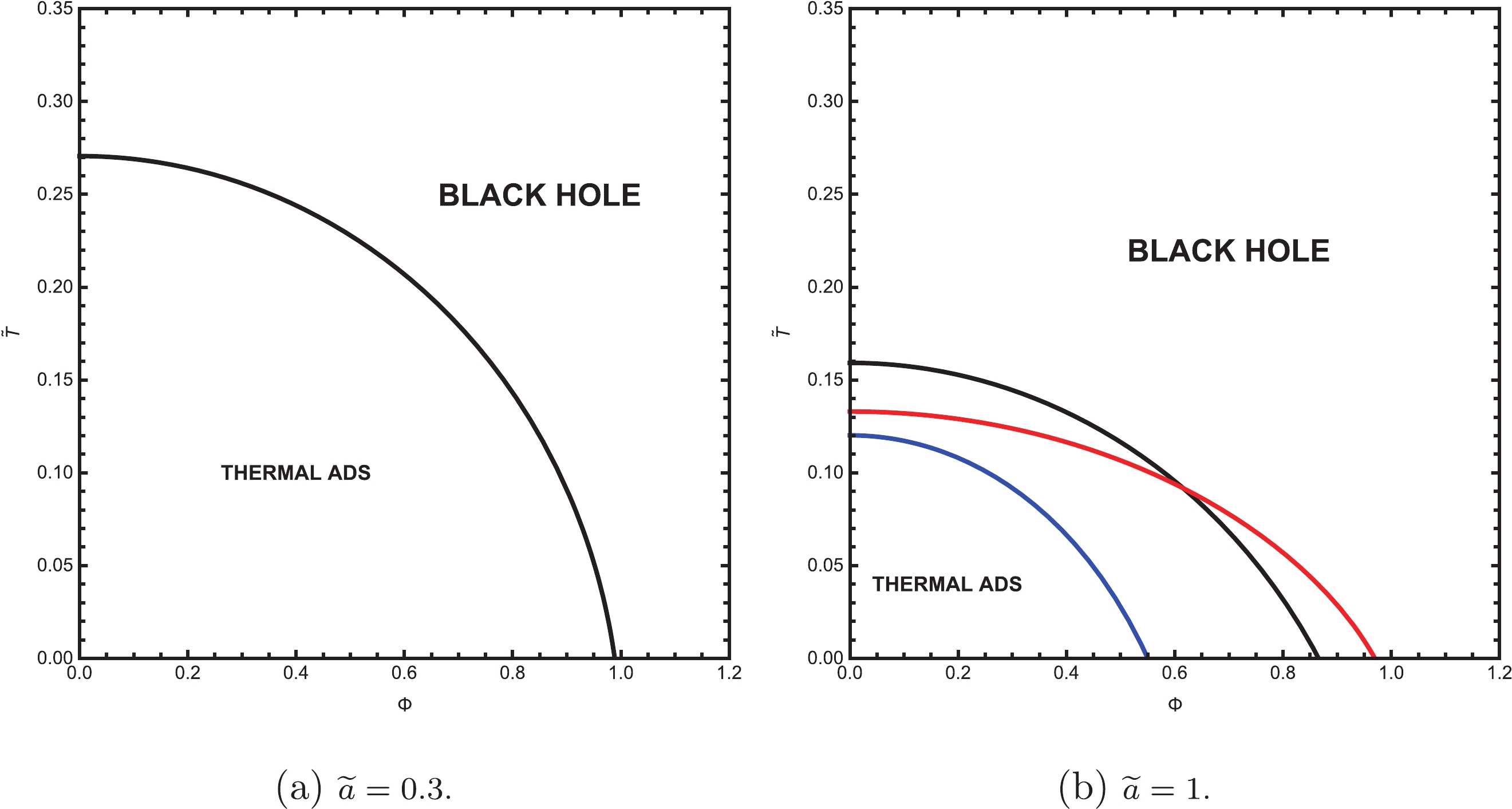
Figure 4. (color online) Phase diagrams in
$ \widetilde{T}-\Phi $ space for various$ \omega $ and$ \widetilde{a} $ . Blue curve:$ \omega = -2/5 $ . Black curve:$ \omega = -2/3 $ . Red curve:$ \omega = -9/10 $ . The first-order phase transitions occur on these curves, causing them to become the dividing lines of the two phases. -
In this section, we investigate the RN black hole surrounded by quintessence dark energy in a cavity. The action with a time-like boundary
$ \partial {\cal{M}} $ on a four dimensional spacetime manifold$ {\cal{M}} $ is$ \begin{aligned}[b] {\cal{S}} =& \frac{1}{16\pi}\int_{{\cal{M}}}{\rm d}^4 x\left(\sqrt{-g}[R-F^{\mu\nu}F_{\mu\nu}]+{\cal{L}}_{q}\right)\\&-\frac{1}{8\pi}\int_{\partial {\cal{M}}}{\rm d}^3 x\sqrt{-\gamma}\left(K-K_0\right). \end{aligned}$

(13) The counter term above is the Gibbons-Hawking-York surface term. K is the extrinsic curvature,
$ \gamma $ is the metric on the boundary, and$ K_{0} $ is a subtraction term to make the Gibbons-Hawking-York term vanish in flat spacetime. When the metric on$ \partial {\cal{M}} $ is fixed, the Gibbons-Hawking-York term is crucial to obtain the correct equations of motion from performing the variation [28]. We can obtain the quintessence RN black hole solution from the action (13)$ {\rm d}s^2 = f(r){\rm d}t^2-\frac{{\rm d}r^2}{f(r)}-r^2({\rm d}\theta^2+{\rm sin}^2 \theta {\rm d}\phi^2), $

(14) and
$ f(r) = 1-\frac{2M}{r}+\frac{Q^2}{r^2}-\frac{a}{r^{3\omega+1}}. $

(15) Suppose that the wall of the cavity surrounding the black hole is located at
$ r_{B} $ . For such a system in a grand canonical ensemble, the wall is maintained at a temperature T and a potential$ \Phi $ . The charge Q of the system is defined as equal to the black hole charge without the cavity and the entrophy S of the system is defined as equal to a quarter of the event horizon area of the black hole$ S = \pi r_{h}^2 $ . For such a system, the total energy can be written as [72]$ E = r_B\left[1-\sqrt{f(r_B)}\right]. $

(16) We define the temperature as
$ T = \left(\frac{\partial E}{\partial S}\right)_{Q} = \frac{T_h}{\sqrt{f(r_B)}} = \frac{1}{4\pi r_h \sqrt{f(r_B)}}\left(1-\frac{Q^2}{r_h^2}+\frac{3a\omega}{r_h^{3\omega+1}}\right), $

(17) where
$ T_h $ is the Hawking temperature of the black hole, and we have used$ r_+ $ to eliminate M$ M = \frac{r_h}{2}+\frac{Q^2}{2r_h}-\frac{a}{2r_h^{3\omega}}. $

(18) The potential is defined as
$ \Phi = \left(\frac{\partial E}{\partial Q}\right)_{S} = \frac{Q\left(\dfrac{1}{r_h}-\dfrac{1}{r_B}\right)}{\sqrt{f\left(r_B\right)}}. $

(19) With all these quantities above, the first law of thermodynamics can thus be written as
$ {\rm d}E = T{\rm d}S+\Phi {\rm d}Q. $

(20) The free energy can be given by
$ F = E-TS-\Phi Q. $

(21) Physical quantities in units of
$ r_B $ can be concise:$\begin{aligned}[b]& x = r_h/r_B,\;\;\;\ \widetilde{a} = a/r_{B}^{3\omega+1},\;\;\;\ \widetilde{Q} = Q/r_B, \\& \ \widetilde{T} = 16\pi r_B T,\;\;\;\ \widetilde{F} = F/r_B. \end{aligned} $

(22) Plugging Eq. (22) into Eq. (21), we can obtain the specific expression for free energy:
$ \widetilde{F} = 1-\sqrt{1-\widetilde{a}-x+\widetilde{Q}^2-\frac{\widetilde{Q}^2}{x}+\frac{\widetilde{a}}{x^{3\omega}}}-\frac{\widetilde{T} x^2}{16}-\Phi \widetilde{Q}. $

(23) Similarly, temperature and potential can be written in units of
$ r_B $ $ \widetilde{T} = \frac{4}{ x\sqrt{1-\widetilde{a}-x+\widetilde{Q}^2-\dfrac{\widetilde{Q}^2}{x}+\dfrac{\widetilde{a}}{x^{3\omega}}}}\left(1-\frac{\widetilde{Q}^2}{x^2}+\frac{3\widetilde{a}\omega}{x^{3\omega+1}}\right) $

(24) and
$ \Phi = \frac{\widetilde{Q}(1/x-1)}{\sqrt{1-\widetilde{a}-x+\widetilde{Q}^2-\dfrac{\widetilde{Q}^2}{x}+\dfrac{\widetilde{a}}{x^{3\omega}}}}. $

(25) However, there are some constraints on the physical quantities of the black hole, which can be presented in
$ x-\widetilde{Q} $ space. First,$ x\leqslant 1 $ apparently holds because the horizon radius$ r_{+} $ is less than cavity radius$ r_{B} $ . On the one hand, we need to ensure that the temperature$ \widetilde{T} $ is not less than zero, which gives$ \widetilde{Q}^2\leqslant x^2+3\widetilde{a}\omega x^{1-3\omega}. $

(26) Note that
$ \widetilde{Q}^2 = x^2+3\widetilde{a}\omega x^{1-3\omega} $ means the emergence of an extreme black hole. On the other hand, all physical quantities must be real numbers, and thus,$ f(r_B)>0 $ needs to be satisfied, which gives$ \widetilde{Q}^2<\frac{(1-\widetilde{a})x-x^2+\widetilde{a} x^{1-3\omega}}{1-x}. $

(27) The above formula should be changed into
$ \widetilde{Q}^2<1+3\widetilde{a}\omega $ when$ x = 1 $ . To simplify the calculation without loss of generality, we set$ \omega = -2/3 $ and only consider the case of$ \widetilde{Q}>0 $ because the constraints of$ \widetilde{Q} $ on x are symmetric. The physically allowed regions in$ x-\widetilde{Q} $ space are displayed in Fig. 5, which are divided into three categories according to the value of$ \widetilde{a} $ . For$ \omega = -2/3 $ , the expression for Boundary I is$ \widetilde{Q} = 0 $ , that for Boundary II is$ x = 1 $ , that for Boundary III is$ \widetilde{Q} = \sqrt{x-\widetilde{a}x-\widetilde{a}x^2} $ , and that for Boundary IV is$ \widetilde{Q} = \sqrt{x^2-2\widetilde{a}x^3} $ . There is no Boundary III in Fig. 5(a) because it is outside Boundary IV. Moreover, no Boundary II is in Fig. 5(c) because the upper limit is$ x = (1-\widetilde{a})/\widetilde{a} $ instead of$ x = 1 $ .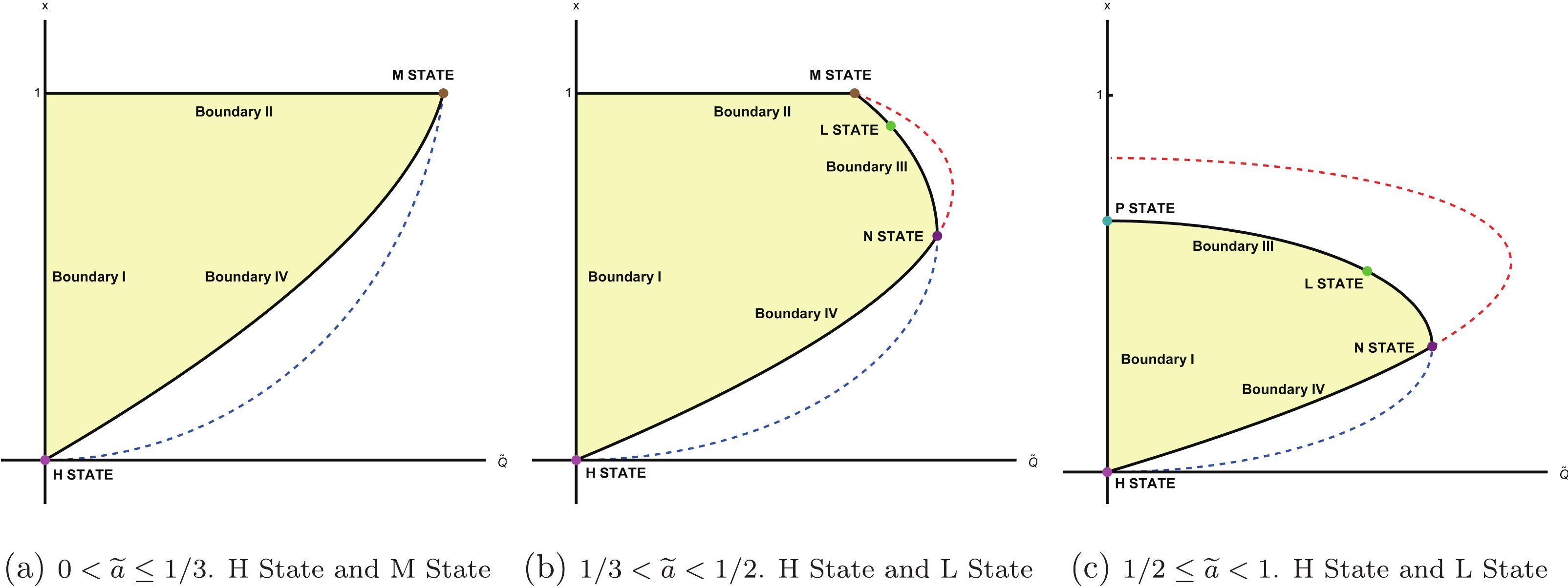
Figure 5. (color online) Three types of distinct physically allowed regions in
$ x-\widetilde{Q} $ space. The yellow area is physically allowed and the black curve is the boundary. The coordinates of these states are H State (0,0), M State ($ \sqrt{1-2\widetilde{a}} $ ,1), N State ($ \frac{1}{2} \sqrt{\widetilde{a}+\frac{1}{\widetilde{a}}-2},\frac{1-\widetilde{a}}{2 \widetilde{a}} $ ), L State (on Boundary III), and P State ($ 0,\frac{1-\widetilde{a}}{\widetilde{a}} $ ).Our strategy to study the phase structures and transitions is as follows. First, we use Eq. (25) to express
$ \widetilde{Q} = \widetilde{Q}(x,\Phi) $ and substitute it into Eq. (24) and Eq. (23), respectively. Therefore, we have$ \widetilde{T}(x,\Phi) $ and$ \widetilde{F}(x,\widetilde{T},\Phi) $ . Again, substituting the above$ \widetilde{T}(x,\Phi) $ into$ \widetilde{F}(x,\widetilde{T},\Phi) $ , we obtain$ \widetilde{F}(x,\Phi) $ . With x as the parameter,$ \widetilde{F}-\widetilde{T} $ diagrams for fixed$ \Phi $ can thus be plotted. However, those$ \widetilde{F}-\widetilde{T} $ curves are the cases that belong to the black hole solution. We have not considered the cases for the boundaries. The situation of each boundary is different, and we need to determine the lowest free energy on each boundary when the grand canonical ensemble parameters$ \widetilde{T} $ and$ \Phi $ are fixed.On Boundary I, that is,
$ \widetilde{Q} = 0 $ , we notice that$ \frac{\partial \widetilde{F}}{\partial \widetilde{Q}}\bigg|_{\rm Boundary\;I} = -\Phi<0, $

(28) which implies that on the boundary other than
$ (0, 0) $ , points with lower free energy can be found in the physically allowed region because the points on the right of$ (0,0) $ are beyond the physically allowed region. We refer to$ (0, 0) $ as the H state, which might be a candidate with the globally lowest free energy.On Boundary II, that is,
$ x = 1 $ , which implies that the cavity merges with the event horizon, we find that$ \frac{\partial \widetilde{F}}{\partial \widetilde{Q}}\bigg|_{\rm Boundary\;II} = -\Phi<0. $

(29) This indicates that on that boundary, the free energy will decrease as
$ \widetilde{Q} $ increases, so the point with the lowest free energy is the right endpoint, which is denoted by M State. In M State, the black hole is an extremal black hole and the cavity merges with the event horizon.On Boundary III, that is,
$ \widetilde{Q} = \sqrt{x-\widetilde{a}x-\widetilde{a}x^2} $ , the free energy of this boundary can be written as$ \widetilde{F} = 1-\frac{ x^2\widetilde{T}}{16}-\Phi \sqrt{x-\widetilde{a} x-\widetilde{a} x^2}. $

(30) If
$ \widetilde{T} $ and$ \Phi $ are determined, the globally minimal free energy on this boundary is also determined because it is only the function of x. Nevertheless, what we really need is that when$ \Phi $ is fixed, the globally minimal free energy of the boundary changes with temperature$ \widetilde{T} $ . To solve this problem, we perform the following deduction:$ \frac{\partial \widetilde{F}(x,\widetilde{T},\Phi)}{\partial x} = 0 \Longrightarrow \widetilde{T}(x,\Phi) = \frac{4\Phi (2 \widetilde{a} x+\widetilde{a}-1)}{x \sqrt{x-\widetilde{a} x-\widetilde{a} x^2}}. $

(31) Substituting this into Eq. (30), we obtain
$ \widetilde{F}(x,\Phi) = 1+\frac{\Phi (2\widetilde{a}x^{2}+3\widetilde{a}x-3x)}{64 \pi \sqrt{x-\widetilde{a} x-\widetilde{a} x^2}}. $

(32) With x as the parameter,
$ \widetilde{F}-\widetilde{T} $ curves for fixed$ \Phi $ can be plotted. It is worth noting that the above equations can only describe the behavior of stagnation points on the boundary, and thus, the endpoints are supposed to be considered because there is no singularity for$ \widetilde{F}(x,\Phi) $ on Boundary III. For the case shown in Fig. 5(b),$ (1-\widetilde{a})/2\widetilde{a}< $ $ x<1 $ . We denote$ x = (1-\widetilde{a})/2\widetilde{a} $ as N State and$ x = 1 $ as M State, and the point between M State and N State may also be the candidate of globally minimal free energy, which is denoted as L State. For the case shown in Fig. 5(c),$ (1-\widetilde{a})/2\widetilde{a}<x<(1-\widetilde{a})/\widetilde{a} $ . We denote$ x = (1-\widetilde{a})/\widetilde{a} $ as P State and L State between P State and N State may have the locally minimal free energy. In N State, the black hole is an extremal black hole, and the cavity merges with the outer event horizon. In L State, the cavity merges with the outer event horizon. In P State, the charge of the black hole equals zero, and the cavity merges with the outer event horizon.On Boundary IV, that is,
$ \widetilde{Q} = \sqrt{x^2-2\widetilde{a}x^3} $ , the black hole is an extremal black hole. In the previous discussion, we have actually reached such a conclusion that Boundary IV belongs to the black hole solution, and that is why Eq. (26) can take the equals sign. Therefore, Boundary IV does not need to be considered again and the globally free energy on the boundary can only be the endpoints, namely H State or M State in Fig. 5(a) and H State or N State in Fig. 5(b) and Fig. 5(c).Once again, we use the heat capacity at constant potential
$ C_{\Phi} $ to judge thermal stability. As discussed before,$ C_{\Phi}>0 $ and$ C_{\Phi}<0 $ correspond to stable and unstable states, respectively. Using$ \widetilde{T}(x,\widetilde{Q}) $ and$ \Phi(x,\widetilde{Q}) $ in Eqs. (24) and (25) to eliminate$ \widetilde{Q} $ , we obtain the expression of x against$ \widetilde{T} $ and$ \Phi $ , which is plotted in Fig. 6. We divide it into three cases in advance, and each case corresponds to a subgraph.
Figure 6. (color online) Plots of x against
$ \widetilde{T} $ for different$ \widetilde{a} $ and$ \Phi $ . The Small BH branches with a negative slope are unstable states while the Large BH branches are stable with a positive slope.In addition, we find there are nine regions in
$ \Phi-a $ phase diagram, as shown in Fig. 7. To obtain the detailed information about the phase structures and transitions of each region, we display the$ \widetilde{F}-\widetilde{T} $ diagrams of the physically allowed regions and the candidates on the boundaries in Fig. 8. The specific and representative cases for each region are selected, and the subsequent analyses are as follows.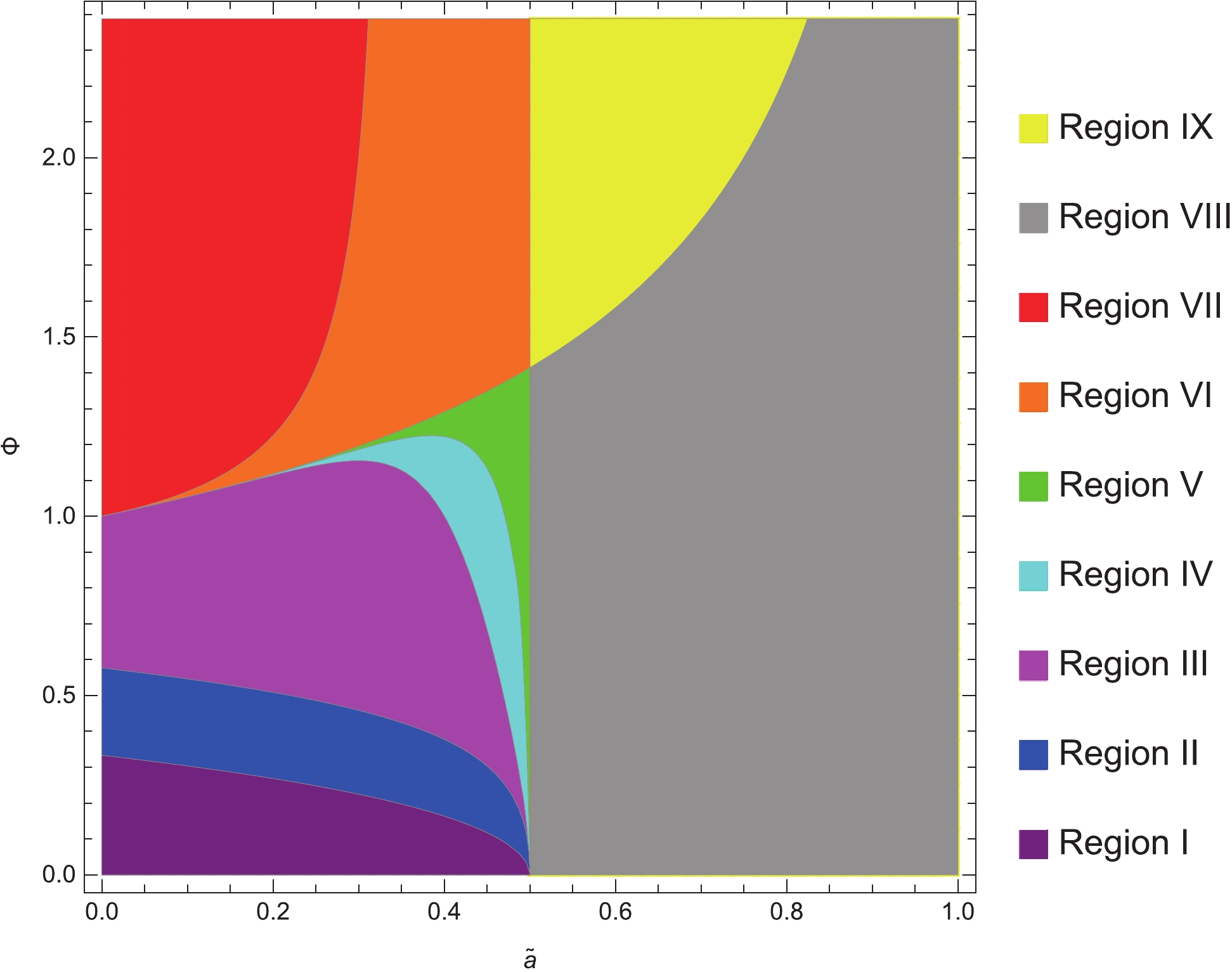
Figure 7. (color online) Nine regions in
$ \Phi-\widetilde{a} $ phase space.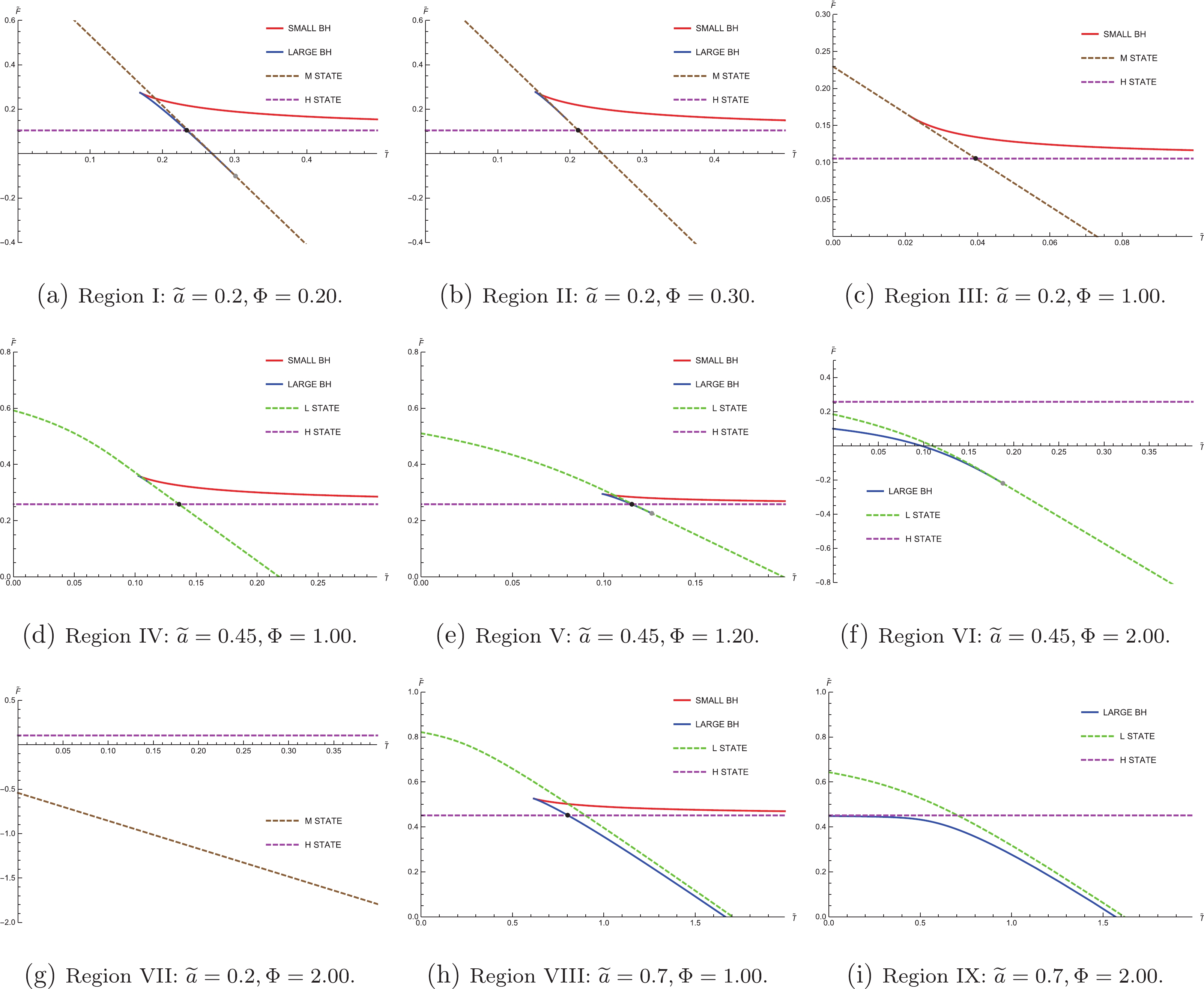
Figure 8. (color online) Plots of free energy
$ \widetilde{F} $ against temperature$ \widetilde{T} $ in nine regions. The black dot is where a first-order phase transition occurs while the gray dot is where a second-order phase transition occurs. The solid lines represent the physically allowed region, and the dashed lines represent the boundaries.For Region I, the
$ \widetilde{F}-\widetilde{T} $ diagram is plotted in Fig. 8(a), and the corresponding physically allowed region is shown in Fig. 5(a). As discussed before, H State and M State are the candidates for minimal free energy on the boundary. Therefore, one can plot the free energy of H State, M State, and the locally stationary points in the physically allowed region against temperature. There are two branches for the physically allowed region, Small BH and Large BH, which connotes that there are both a locally maximal and a locally minimal free energy in that region. When temperature$ \widetilde{T} $ is small, H State has the minimal free energy; thus, it is the globally stable state. When temperature continues to rise, a first-order phase transition occurs from H State to Large BH, and the latter becomes the thermodynamical preferred state. As$ \widetilde{T} $ increases further, a second-order phase transition occurs; then, M State becomes the stablest state.For Region II, the
$ \widetilde{F}-\widetilde{T} $ diagram is plotted in Fig. 8(b). Compared with Region I, only the value of$ \Phi $ changes in this region; thus, the candidates remain unchanged since the physically allowed region stays the same. However, the difference is that the free energy of the point where Large BH tangent to M State is higher than that of the first-order transition, resulting in only the first-order transition from H State to M State occuring in this region.For Region III, the
$ \widetilde{F}-\widetilde{T} $ diagram is plotted in Fig. 8(c), from which one can see that only the Small BH branch is in the physically allowed region. This just corresponds to the case$ \Phi = 50 $ in Fig. 6(a). As$ \widetilde{T} $ increases, there is only a first-order phase transition occurring from H State to M State.For Region IV, the
$ \widetilde{F}-\widetilde{T} $ diagram is plotted in Fig. 8(d), of which the physically allowed region is displayed in Fig. 5(b) and the$ x-\widetilde{T} $ diagram is plotted in Fig. 6(b). It is distinct from the case shown in Region II, mainly because the locally minimal free energy on the boundary lies at L State, which is between M State and N State. We can see from Fig. 8(d) that L State is actually a combination of a curve and a straight line. The curve corresponds to the movement of L State on Boundary III, while the straight line corresponds to L State coinciding with M State. When the temperature$ \widetilde{T} $ rises, the black hole undergoes a first-order phase transition from H State to L State.For Region V, the
$ \widetilde{F}-\widetilde{T} $ diagram is plotted in Fig. 8(e). Unlike in Region IV, in this region, the free energy of the point where Large BH is tangential to L State is lower than that of the first-order transition, resulting in the addition of a second-order transition from Large BH to L State. In general, a first-order phase transition and a second-order phase transition occur sequentially in this region.For Region VI, the
$ \widetilde{F}-\widetilde{T} $ diagram is plotted in Fig. 8(f). There is only the Large BH branch for the physically allowed region, which can also be realized from Fig. 6(b). As$ \widetilde{T} $ increases, a second-order phase transition occurs from Large BH to L State.For Region VII, the
$ \widetilde{F}-\widetilde{T} $ diagram is plotted in Fig. 8(g) and the physically allowed region is shown in Fig. 5(a). Notably, no phase transition occurs in this region. In this case, only the point that has the minimal free energy on the boundary might be the globally stable state, on account of Eqs. (24) and (25) without real roots in the physically allowed region. It also implies that it is impossible to find an$ x-\widetilde{T} $ curve in Fig. 6(a), and hence, there are only three corresponding curves for four regions.For Region VIII, the
$ \widetilde{F}-\widetilde{T} $ diagram is plotted in Fig. 8(h). As$ \widetilde{T} $ increases, a first-order transition occurs from H State to Large BH. This region is very similar to Region V, but the difference is that no second-order phase transition occurs because the Large BH line and L State line will never intersect.For Region IX, the
$ \widetilde{F}-\widetilde{T} $ diagram is plotted in Fig. 8(i). This region is a deformation of Region VI, and it is very similar to Region VIII in that when$ \widetilde{T} $ tends to infinity, the Large BH branch and the L State line approach infinitely but never intersect, and thus, no phase transition occurs.In summary, as
$ \widetilde{T} $ increases, a first-order phase transition occurs in Regions II, III, IV, and VIII, a second-order phase transition occurs in Region VI, a first-order and a second-order phase transition occur successively in Region I and Region V, and no phase transition occurs in Regions VII and IX. In Fig. 7, one can refer to$ L_{i,i+1} $ as the critical line between Region i and Region$ i+1 $ . As$ \widetilde{a} $ increases,$ L_{34} $ ,$ L_{45} $ ,$ L_{56} $ , and$ L_{67} $ originate from the same$ \Phi $ and gradually diverge. Meanwhile, the value of$ \Phi $ on$ L_{12} $ ,$ L_{23} $ ,$ L_{34} $ and$ L_{45} $ decreases and converges to zero as$ \widetilde{a}\rightarrow 0.5 $ . It is worth noting that the straight line$ \widetilde{a} = 0.5 $ divides the original$ L_{56} $ into the current$ L_{56} $ and$ L_{89} $ . This is because, when$ \widetilde{a}>0.5 $ , the Large BH branches tend to infinity and never intersect with L State lines as$ \widetilde{T} $ rises, as explained before. However, for the general case, if$ 1+3\widetilde{a}\omega<0 $ , M State disappears, and the Large BH branches of the physically allowed region never intersect with L State lines as$ \widetilde{T} $ rises, which leads to the disappearance of the second-order phase transition. Equivalently, the equation of the vertical line in the$ \Phi-\widetilde{a} $ diagram is$ \widetilde{a} = -1/3\omega. $

(33) It is intriguing to plot the
$ \widetilde{T}-\Phi $ phase diagrams to conclude the conclusions above. As shown in Fig. 9, we set$ \widetilde{a} = 0.45 $ and$ 0.7 $ , respectively. In Fig. 9(a), there are three potential phases with the lowest free energy. When$ \Phi<\Phi_{c1}\approx0.12 $ , H State, Black Hole, and L State in turn become the globally stable state as$ \widetilde{T} $ increases. When$ \Phi_{c1}<\Phi<\Phi_{c2}\approx1.13 $ , only H State and L State have the globally lowest free energy with the change in$ \widetilde{T} $ . When$ \Phi_{c2}<\Phi<\Phi_{c3}\approx1.35 $ , the three phases become the candidates of lowest free energy again. Significantly, as$ \Phi $ rises to$ \Phi_{c3} $ , the first-order phase transition line between H State and Black Hole will become almost a vertical line. It corresponds to the transition between Region V and Region VI; that is, when$ \Phi $ increases by a small amount,$ \widetilde{T} $ decreases sharply. In Fig. 9(b), there are only two potential phases with the lowest free energy. As$ \Phi $ rises to$ \Phi_{c4}\approx1.83 $ ,$ \widetilde{T} $ decreases rapidly, which corresponds to the transition between Region VIII and Region IX.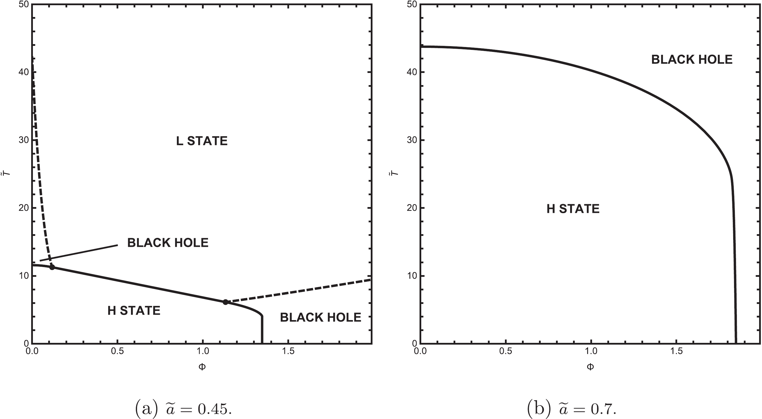
Figure 9. Phase diagrams in
$ \widetilde{T}-\Phi $ space for different$ \widetilde{a} $ . A first-order phase transition occurs on the solid curve and a second-order phase transition occurs on the dashed curve. The black dot is the intersection of the two curves. -
In this paper, we considered a grand canonical ensemble and studied the phase structures and transitions of an RN black hole surrounded by quintessence dark energy in AdS space and in a cavity, separately. For the quintessence RN-AdS black hole, we fixed the temperature and the potential and found that for some temperatures, there are two branches of the black hole, namely Small BH and Large BH. By calculating the heat capacity at constant potential, we discovered that the Small BH branch is unstable, whereas the Large BH is stable. Furthermore, a first-order transition occurred as temperature increased for some small values of
$ \Phi $ instead of large$ \Phi $ . Thus, we divided all the cases into two regions in the$ \Phi-\widetilde{a} $ phase diagram in Fig. 2, in which one point can decide whether a phase transition occurs or not. Moreover, a$ \widetilde{T}-\Phi $ phase diagram is displayed in Fig. 4.Moreover, we investigated the phase structures and transitions of the black hole in another boundary condition, i.e., the Dirichlet wall. Initially, we used the energy of the system obtained in [72] to construct the first law of thermodynamics. The case for the barotropic index
$ \omega = -2/3 $ was studied in detail. Moreover, we obtained the constraints of black hole parameters x and$ \widetilde{Q} $ in a cavity, which were separated into three cases depending on the value of$ \widetilde{a} $ . In the physically allowed region, we obtained the$ \widetilde{F}-\widetilde{T} $ curves for fixed$ \Phi $ with x as the parameter. On the boundary, the position of the latent lowest free energy was evaluated through the expression of$ \widetilde{F} $ , and we labeled these points in the$ x-\widetilde{Q} $ space as different states. Finally, we plotted the$ \widetilde{F}-\widetilde{T} $ diagrams and obtained the phase transitions. In summary, there are nine regions with different phase structures. To distinguish them more clearly, we plotted the nine regions in the$ \Phi-\widetilde{a} $ phase diagram in Fig. 7. The$ \widetilde{T}-\Phi $ phase diagrams were also plotted in Fig. 9, in which the phase structures for fixed$ \omega $ and$ \widetilde{a} $ could be displayed clearly. The discrepancy in the phase structures and transitions of a quintessence RN black hole between the two different boundary conditions is distinct. -
We are grateful to Hanwen Feng, Wei Hong, Peng Wang, and Mingtao Yang for useful discussions and valuable comments.
Phase structures and transitions of quintessence surrounding RN black holes in a grand canonical ensemble
- Received Date: 2020-11-17
- Available Online: 2021-07-15
Abstract: Considering a grand canonical ensemble, we study the phase structures and transitions of RN black holes surrounded by quintessence dark energy on two different boundary conditions, namely AdS space and a Dirichlet wall. For AdS space, under the condition of fixed temperature and potential, as the temperature increases for lower potential, the black hole undergoes a first-order phase transition, while for higher potential, no phase transition occurs. There are two different regions in the parameter space. For the Dirichlet wall, on which the temperature and potential are fixed, the state parameter of quintessence


 DownLoad: