


 Abstract
 HTML
HTML Reference
 Related
 PDF
PDF


-
The perturbations of black holes are powerful probes to disclose their stability, and have been studied intensively for decades. The linear (in)stability of a black hole can be characterized by its quasi-normal modes (QNMs). If the imaginary part of the QNMs is positive, the perturbation amplitude will grow exponentially, implying instability. The QNMs provide the fingerprints of black holes and are related to gravitational wave observations [1, 2]. In four-dimensional spacetime, black holes, including Schwarzschild black holes, Reissner–Nordström (RN) black holes and Kerr black holes, are stable under neutral scalar, electromagnetic field or gravitational perturbations in general [1, 2], regardless of whether the black holes are in asymptotically flat, de Sitter (dS) or anti-dS (AdS) spacetimes. The case for Kerr-Newman spacetime is subtle due to the difficulty of decoupling the variables. Numerical works strongly support that they are stable [3, 4]. But this problem has not been settled. However, four-dimensional black holes can be unstable if superradiance occurs [5-8]. Perturbations in higher dimensional spacetimes and alternative theories of gravity have also attracted a lot of attention [9-18].
Recently, a regularized four-dimensional (4D) Einstein-Gauss-Bonnet (EGB) gravity theory was proposed [19], in which the Gauss-Bonnet coupling constant was rescaled with
$ \alpha\to\alpha/(D-4) $ in the limit$ D\to4 $ , and novel black hole solutions were found [20-36]. This has stimulated a lot of studies, as well as doubts [37-78]. Fortunately, some proposals have been raised to circumvent the issues of the regularized 4D EGB gravity, including adding an extra degree of freedom to the theory [37-43], or breaking the temporal diffeomorphism invariance [44, 45], where a well-defined theory can be formulated. The regularized black hole solutions can still be derived from these more rigorous routes. Therefore, it is worth studying the perturbations of these black hole solutions. In fact, the stability of regularized four-dimensional black holes has been studied from many aspects [46-59], of which most focused only on the neutral cases. We studied the charged massless scalar perturbations in regularized 4D charged EGB black holes with asymptotically flat and dS spacetimes in Refs. [60, 61], respectively. It was found that the charged massless scalar perturbations in asymptotically flat spacetime are always stable, while those in asymptotically dS spacetime suffer from a new kind of test field instability where not all the modes satisfying the superradiant condition are unstable.Since the boundary conditions in AdS spacetime are different from those in asymptotically flat or dS spacetimes, it can be expected that the behaviors of perturbations of black holes in AdS spacetime will be different from those in flat or dS spacetime. Therefore, in this paper we study the charged scalar perturbation in a regularized 4D charged black hole in AdS spacetime. We find that the asymptotic iteration method used in Refs. [60, 61] does not work well here. Instead, we adopt another numerical method to calculate the frequencies of the perturbations. The QNMs are worked out as a generalized eigenvalue problem and the results are checked by the time-evolution method. We find that the charged massless scalar suffers from linear instability. However, unlike the dS case, all unstable modes here satisfy the superradiant condition. The effects of the Gauss-Bonnet coupling constant, the black hole charge, the scalar charge and the cosmological constant are analyzed in detail.
This paper is organized as follows. In Section II, we describe the regularized 4D charged EGB black hole in AdS spacetime and the parameter region allowing an event horizon of the black hole. In Section III we elaborate the method to calculate the quasinormal modes of the charged scalar perturbation in a regularized charged black hole. In Section IV, we study in detail the effects of the Gauss-Bonnet coupling constant, the black hole charge, the scalar field charge and the cosmological constant on the QNMs. Section V then gives some discussion.
-
In spherically symmetric spacetime, the electrovacuum solution of the four-dimensional EGB gravity in AdS spacetime is given by [20]
$ {\rm d}s^{2} = -f(r){\rm d}t^{2}+\frac{1}{f(r)}{\rm d}r^{2}+r^{2}({\rm d}\theta^{2}+\sin^{2}\theta {\rm d}\phi^{2}), $

(1) where the metric function is:
$ f(r) = 1+\frac{r^{2}}{2\alpha}\left(1-\sqrt{1+4\alpha\left(\frac{M}{r^{3}}-\frac{Q^{2}}{r^{4}}+\frac{\Lambda}{3}\right)}\right), $

(2) and the gauge potential is:
$ A = -\frac{Q}{r}{\rm d}t. $

(3) Here,
$ M,\,Q $ are the mass and charge of the black hole, respectively. In Eq. (2) the cosmological constant is$ \Lambda = -3/l^2 $ , where l is the cosmological radius. As$ r\to\infty $ , the solution approaches an asymptotically AdS spacetime if$ \frac{1}{2\alpha} \left( 1-\sqrt{1+\frac{4\alpha\Lambda}{3}} \right)>0. $

(4) This condition can be satisfied only for negative
$ \Lambda $ , no matter whether$ \alpha $ is positive or negative. When$ \alpha\to0 $ , the solution goes back to the RN-AdS black hole. Note that the solution (1) coincides formally with those obtained from conformal anomaly and quantum corrections [79-81] and from Horndeski theory [37-43].We fix the black hole event horizon
$ r_{+} = 1 $ in this paper. To ensure$ f(r_+) = 0 $ , it is required that$ \alpha>-1/2 $ . The mass M can be expressed as:$ M = \frac{1}{3} \left(3 \alpha -\Lambda +3 Q^2+3\right). $

(5) The parameter region that allows the existence of a black hole with positive Hawking temperature on the event horizon is determined by
$ f'(r_+)>0 $ . This leads to an inequality which is very similar to the case in dS spacetime [61]:$ Q^2 + \alpha + \Lambda <1. $

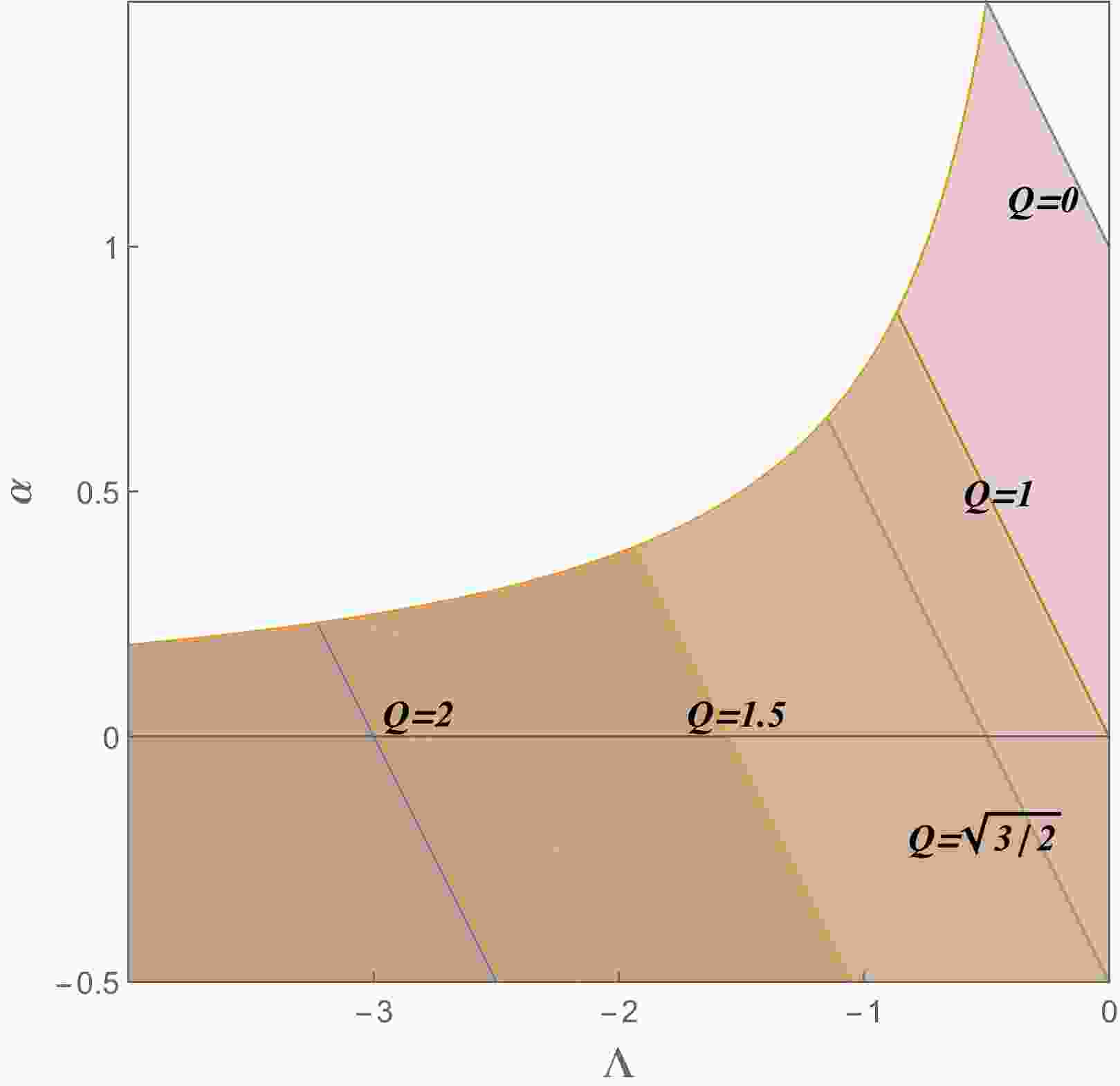
(6) The region plot of the allowed parameter region is given in Fig. 1, from which we find that the allowed region (shaded region) shrinks with increasing Q. However, unlike the case in dS spacetime, the black hole charge Q is unbounded in asymptotically AdS spacetime here.
Figure 1. (color online) Parameter region that allows the existence of a black hole with metric function (2). The allowed region for a larger Q is a subset of that for a smaller Q.
-
We study the linear stability of a massless charged scalar perturbation
$ \psi $ in the black hole solution (1). It is known that fluctuations of order$ O(\epsilon) $ in the scalar field in a given background induce changes in the spacetime geometry of order$ O(\epsilon^2) $ [5]. To leading order, we can study the perturbations on the fixed background geometry that satisfies:$ D_\mu D^\mu \psi = 0, $

(7) where
$D_\mu \equiv \nabla_\mu - {\rm i}eA_\mu$ , and e is the charge of the test scalar field.It is more convenient to work under the ingoing Eddington-Finkelstein coordinate,
$ v = t + r_*, $

(8) when studying the time evolution of the perturbation. Here
$ r_* $ is the tortoise coordinate defined with${\rm d}r_* = {\rm d}r/f$ . In this coordinate, the line element becomes:$ {\rm d}s^2 = -f {\rm d}v^2 + 2 {\rm d}v{\rm d}r + r^2 {\rm d} \Omega^2_2. $

(9) The Maxwell field in Eddington-Finkelstein coordinates is:
$ A = -\frac{Q}{r} {\rm d}v, $

(10) where we get rid of the spatial component of the gauge field by a gauge transformation.
The equation of motion (7) is separable by taking the following form:
$ \psi = \frac{\phi(v,r)Y_{lm}(\theta,\varphi)}{r}, $

(11) where
$ Y_{lm} $ is the spherical harmonic function. Inserting Eq. (11) into Eq. (7), we have:$ f\partial_r^2 \phi + f' \partial_r \phi - 2{\rm i}e A_v \partial_r \phi - {\rm i}e A'_v \phi + 2\partial_v \partial_r \phi + V(r)\phi = 0, $

(12) where the prime
$ ' $ denotes the derivative with respect to r, and the effective potential is:$ V(r) = -f'(r) /r - l(l+1) /r^2. $

(13) We show the effective potential when
$ l = 0 $ in Fig. 2. When Q and$ \Lambda $ are fixed, the effective potential well becomes shallower as$ \alpha $ increases. When$ \Lambda $ and$ \alpha $ are fixed (the thick lines and dashed lines respectively), the effective potential well becomes shallower as Q increases. When Q and$ \alpha $ are fixed (the thick lines and thin lines respectively), the effective potential becomes deeper as$ \Lambda $ increases. We will see that these behaviors of effective potential are related to the linear instability structure of the massless charged scalar perturbation of the black hole.
Figure 2. (color online) Effective potential when
$ l = 0 $ . The thick lines are for$ Q = 0.6,\Lambda = -0.1 $ , the thin lines are for$ Q = 0.6,\Lambda = -0.3 $ , and the dashed lines are for$ Q = 0.8,\Lambda = -0.1 $ .In order to implement the frequency analysis on Eq. (12), we consider the following mode:
$ \phi(v,r) = \phi(r) {\rm e}^{-{\rm i}\omega v}. $

(14) Then Eq. (12) becomes:
$ f\partial_r^2 \phi + f' \partial_r \phi - 2{\rm i}e A_v \partial_r \phi - {\rm i}e A'_v \phi -2{\rm i}\omega \partial_r \phi + V(r)\phi = 0. $

(15) A more convenient approach for the numerical calculation is to work under the
$ z \equiv r_+ / r $ coordinate, such that we can solve the equation of motion in a bounded region$ z \in [0,1] $ . This coordinate has been widely adopted in solving gravitational background solutions and perturbations [82-85]. Here, the ingoing condition at the horizon is satisfied by setting the time-dependent factor${\rm e}^{-{\rm i} \omega v}$ and requiring a regular$ \phi(r) $ near the horizon. The asymptotic AdS requires a vanishing$ \phi(r) $ at the boundary, which can be realized by extracting$ 1/r $ from$ \phi $ .The next step is to find the QNMs, i.e. the modes with complex frequency
$\omega = \omega_{R} + {\rm i} \omega_{I}$ . When the imaginary part$ \omega_I >0 $ , the perturbation amplitude grows exponentially with time. When the amplitude becomes large enough, the back reaction of the perturbation on the geometry cannot be ignored and implies that the system may become unstable. However, at this stage, the linear approximation adopted in this paper is inadequate and full nonlinear studies are required.The radial equation (15) is generally hard to solve analytically, except for a few instances such as the pure (A)dS spacetimes and Nariai spacetime [1, 2]. Various numerical methods have been developed to obtain the QNMs, such as the WKB method, perturbation method, and iteration methods [86-90].
Recently, a new method has been proposed that re-casts the search for QNMs to a generalized eigenvalue problem by discretizing the equation of motion [91-95]. In this paper, we discretize the spatial coordinate with a Gauss-Lobatto grid with N collocation points. It has been shown that the Gauss-Lobatto grid is an efficient method for solving eigenvalue problems [96]. We examined this in our calculations and found that the Gauss-Lobatto collocation method requires significantly fewer points than the uniform collocation method to achieve the same accuracy. With the discretization, we arrive at a discretized version of Eq. (15),
$ \left({\cal{M}}_0 + \omega {\cal{M}} _1 \right) \vec \phi = 0, $

(16) where
$ {\cal{M}}_{0,1} $ are$ N\times N $ complex-valued matrices and are independent of$ \omega $ . The eigenvalues$ \omega $ in Eq. (16) can be efficiently solved by$ {\texttt{Eigenvalues}}$ [-$ {\cal{M}}_0 $ ,$ {\cal{M}}_1 $ ] with$ {\texttt{Mathematica}}$ . Equivalently, one may also solve the roots of$ \det \left({\cal{M}}_0 + \omega {\cal{M}} _1 \right) = 0 $ to find the eigenvalues. The result is a finite set$ \{\omega\} $ with N elements, of which some are spurious QNMs. The results are reliable only if they are convergent when the collocation density is increased. The fundamental mode is the one with the largest imaginary part. -
We study the linear instability of the massless charged scalar field in the 4D EGB model by showing the relation between the dominant QNMs and the system parameters. We first explore the effect of
$ \alpha, \, Q,\, \Lambda $ and e on the QNMs. After that we study the comprehensive linear instability structure of the massless charged scalar perturbation by showing the stable region in the allowed parameter space. -
In the asymptotic dS case, the effect of
$ \alpha $ on the linear instability depends on the specific values of Q and$ \Lambda $ [61]. It is especially important to find the role the GB coupling constant$ \alpha $ plays in the linear instability structure of the AdS case here.As an example, we fix
$ \Lambda = - 2/3,\,e = 1,\,l = 0 $ , and show the QNMs as a function of$ \alpha $ in Fig. 3. The real part of the fundamental mode,$ \omega_R $ , decreases monotonically with$ \alpha $ . By comparing the curves of different charges Q we find that$ \omega_R $ decreases monotonically with Q. We also find that the imaginary part of the fundamental mode,$ \omega_I $ , first decreases with$ \alpha $ and then increases with$ \alpha $ . The imaginary part$ \omega_I $ increases with Q, indicating that increasing Q may lead to linear instability. However, in Fig. 3, where we have fixed$ e = 1 $ ,$ \omega_I $ is always negative and no linear instability occurs.
Figure 3. (color online)
$ \omega_R $ (left) and$ \omega_I $ (right) of the fundamental mode as a function of$ \alpha $ at$ \Lambda = -2/3,\,e = 1,\,l = 0 $ .We show the fundamental mode as a function of
$ \alpha $ at larger scalar charge$ e = 4 $ in Fig. 4. In this case,$ \omega_R $ still decreases monotonically with$ \alpha $ , as it does when$ e = 1 $ . For the imaginary part, we find that when Q is relatively small,$ \omega_I $ first decreases with$ \alpha $ and then increases with$ \alpha $ (see the blue curve in the right plot of Fig. 4). This is similar to the behaviour with$ e = 1 $ . However, when$ \alpha $ is relatively large,$ \omega_I $ can become positive and lead to linear instability. Therefore, the linear instability occurs only at a large enough value of perturbation charge e. For intermediate values of Q, we find that$ \omega_I $ can increase monotonically with$ \alpha $ . For large values of Q,$ \omega_I $ can decrease with$ \alpha $ for relatively large$ \alpha $ . In addition, both$ \omega_R $ and$ \omega_I $ increase with Q for$ e = 4 $ . The more comprehensive dependence of the linear instability on the scalar charge e is given in subsection IV D.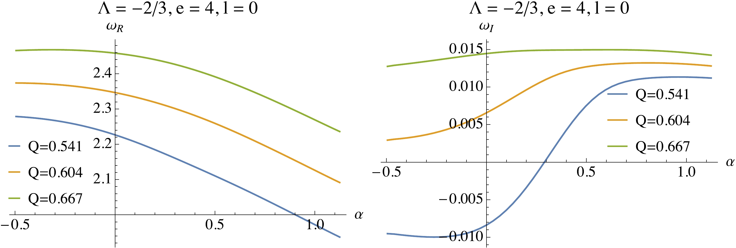
Figure 4. (color online)
$ \omega_R $ (left) and$ \omega_I $ (right) of the fundamental mode as a function of$ \alpha $ at$ \Lambda = - 2/3,\,e = 4,\,l = 0 $ .From the viewpoint of the effective potential shown in Fig. 2, increasing
$ \alpha $ makes the effective potential well shallower. An effective potential barrier appears near the horizon when$ \alpha $ is large enough. The scalar perturbation is harder for the black hole to absorb and can accumulate in the effective potential well. As a consequence, the massless charged scalar field tends to be unstable as$ \alpha $ increases and the imaginary part of the frequency$ \omega_I $ tends to be positive.It has been shown that modes of
$ l>0 $ are usually more stable than those of$ l = 0 $ [61]. In the present model, a similar phenomenon can also be observed. We show the fundamental modes as functions of$ \alpha $ at$ e = 4,\,l = 1 $ in Fig. 5. Comparing Fig. 4 and Fig. 5 we see that$ \omega_I $ for$ l = 1 $ is smaller than that of$ l = 0 $ , which implies that the$ l = 1 $ perturbation mode is indeed more stable than that of$ l = 0 $ mode. For the real part of the fundamental mode, we find that$ \omega_R $ for$ l = 1 $ is larger than that for$ l = 0 $ , which corresponds to a more rapidly oscillating mode.
Figure 5. (color online)
$ \omega_R $ (left) and$ \omega_I $ (right) of the fundamental mode as a function of$ \alpha $ at$ \Lambda = -2/3,\,e = 4,\,l = 1 $ .In this subsection, we find that increasing the coupling constant
$ \alpha $ can lead to linear instability, and this instability occurs only at large enough perturbation charge e. Moreover, the stability is enhanced when the degree l is increased. -
In this subsection, and we explore more comprehensively the relationship between the QNMs and the black hole charge Q. In Fig. 6, as an example, we show the dependence of the QNMs on Q when
$ \alpha = - \dfrac{99}{200},\,e = 1,\,l = 0 $ . We find that both$ \omega_R $ and$ \omega_I $ increase with Q. Especially,$ \omega_I $ can become positive with increasing Q. This means that increasing Q will render the system more unstable and more oscillating. This is in accordance with the observations in the previous subsection.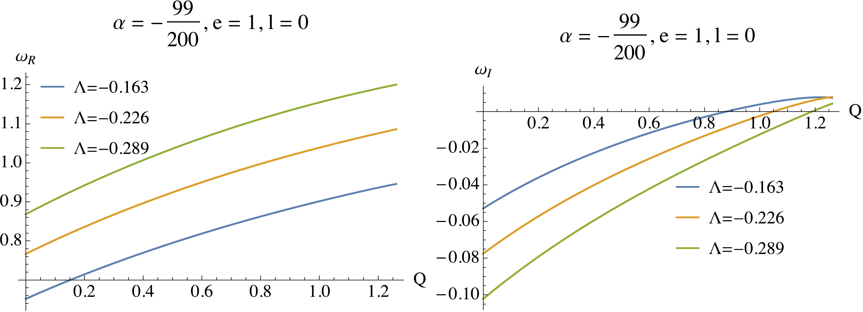
Figure 6. (color online)
$ \omega_R $ (left) and$ \omega_I $ (right) of the fundamental mode as a function of Q at$ \alpha = -99/200,\,e = 1,\,l = 0 $ .Comparing the thick lines and dashed lines in Fig. 2, we see that increasing the black hole charge makes the effective potential at the horizon larger. It is harder for black holes with larger Q to absorb the perturbations. The perturbations can be trapped more easily in the effective potential well. Thus, increasing Q makes the system more unstable.
Also, by comparing the data at different values of
$ \Lambda $ we find that$ \omega_R $ decreases with increasing$ \Lambda $ , while$ \omega_I $ increases with increasing$ \Lambda $ . This phenomenon suggests that decreasing$ \Lambda $ will make the charged massless scalar perturbation more stable and less oscillating. -
We show the QNMs as functions of
$ \Lambda $ when$ Q = 1/10,\,e = 1,\,l = 0 $ in Fig. 7. From the left-hand plot we see that$ \omega_R $ decreases monotonically with$ \Lambda $ . For the imaginary part, when$ |\Lambda| $ is relatively small,$ \omega_I $ is positive and decreases with$ \Lambda $ , and the system is always unstable①. However, when$ \Lambda $ decreases further,$ \omega_I $ reaches its local maximum and then starts to decrease. When$ \Lambda $ is decreased even further,$ \omega_I $ becomes negative and the system becomes stable. This again agrees with the observations in the last subsection that the system becomes more stable and more rapidly oscillating with decreasing$ \Lambda $ . From the potential behaviors in Fig. 2, we see that decreasing$ \Lambda $ makes the effective potential well deeper. The perturbations can be trapped more easily by black holes with larger$ \Lambda $ . Thus, decreasing$ \Lambda $ makes the system more stable. Observing the points where$ \omega_I = 0 $ we also find that the system becomes more stable with increasing$ \alpha $ .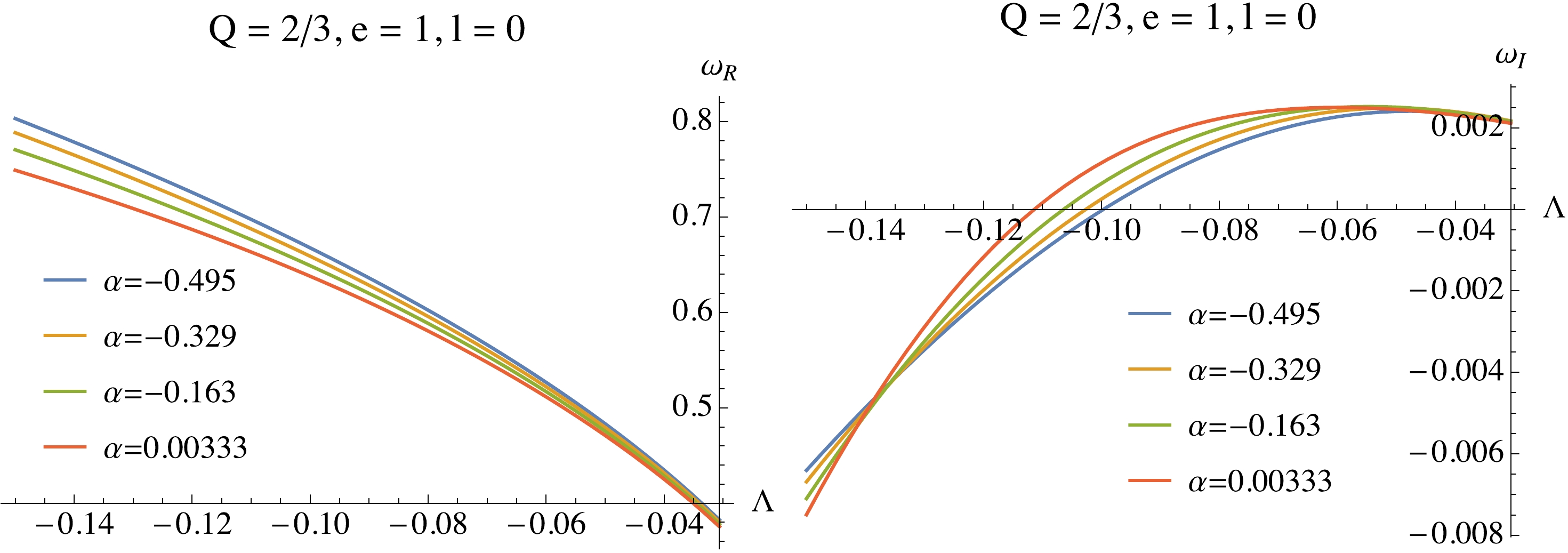
Figure 7. (color online)
$ \omega_R $ (left) and$ \omega_I $ (right) of the fundamental mode as a function of$ \Lambda $ at$ Q = 1/10,\,e = 1,\,l = 0 $ . -
In this subsection, we systematically study the relationship between the linear instability of the charged massless scalar field and the scalar charge e. In principle, the scalar charge e can be either positive or negative. However, here the linear instability structure with negative charge
$ -|e| $ is the same as that of the positive charge$ |e| $ . Inserting the Maxwell field (10) into Eq. (12), we have:$ f\partial_r^2 \phi + f' \partial_r \phi - 2{\rm i}eQ \partial_r \phi/r - {\rm i}eQ \phi/r^2 + 2\partial_v \partial_r \phi + V(r)\phi = 0, $

(17) from which we find that e always appears in pairs with
${\rm i}Q$ , and the other terms contain only$ Q^2 $ . Accordingly, by separating the real and imaginary parts, the discrete eigenvalue equation (16) can be decomposed into the following form:$ \left[ ({{\cal{M}}}^R_0 + {\rm i}\omega_I {{\cal{M}}}_1 ) + {\rm i} ({{\cal{M}}}^I_0 - {\rm i}\omega_R {{\cal{M}}}_1)\right]\vec \phi = 0. $

(18) Here
$ {{\cal{M}}}_1 $ is a purely imaginary matrix because$ \omega $ always comes in pairs with i in Eq. (15) and$ \partial_r $ only contributes a real-valued differential matrix. The conjugate of Eq. (18) becomes:$ \left[ ({{\cal{M}}}^R_0 + {\rm i}\omega_I {{\cal{M}}}_1 ) + {\rm i} (-{{\cal{M}}}^I_0 + {\rm i}\omega_R {{\cal{M}}}_1)\right]\vec \phi^{*} = 0. $

(19) Consequently, performing
$ {{\cal{M}}}^I_0 \to -{{\cal{M}}}^I_0 $ , which can result from performing$ e\to -e $ since$ {\cal{M}}^I_0 $ is linear in e, we obtain a root$-\omega^{*} = -\omega_R + {\rm i} \omega_I$ . Therefore, we prove that when we perform$ e\to -e $ , the imaginary part of the QNMs will be the same, while the real part of the QNMs becomes the opposite of itself. We have also verified this result in our numerical calculation. Figure 8 shows the properties of the QNMs when changing the sign of e. Therefore, we can safely focus on positive e to reveal the linear instability. Next, we present the explicit effect of the perturbation charge e on the QNMs, along$ \alpha,\, Q,\, \Lambda $ .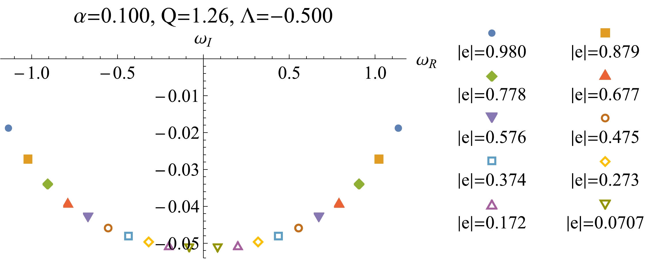
Figure 8. (color online) Fundamental modes for different values of e. Each color or marker corresponds to a pair of e's with an absolute value
$ |e| $ , where the left hand side is$ e = -|e| $ and the right hand side$ e = |e| $ .The phenomena are qualitatively the same along
$ \alpha,\, Q,\, \Lambda $ , which we show in Fig. 9.$ \omega_I $ increases with the increase of e for an arbitrary parameter. Next, we study the comprehensive instability structure by locating the critical surfaces, separating the stable and unstable regions.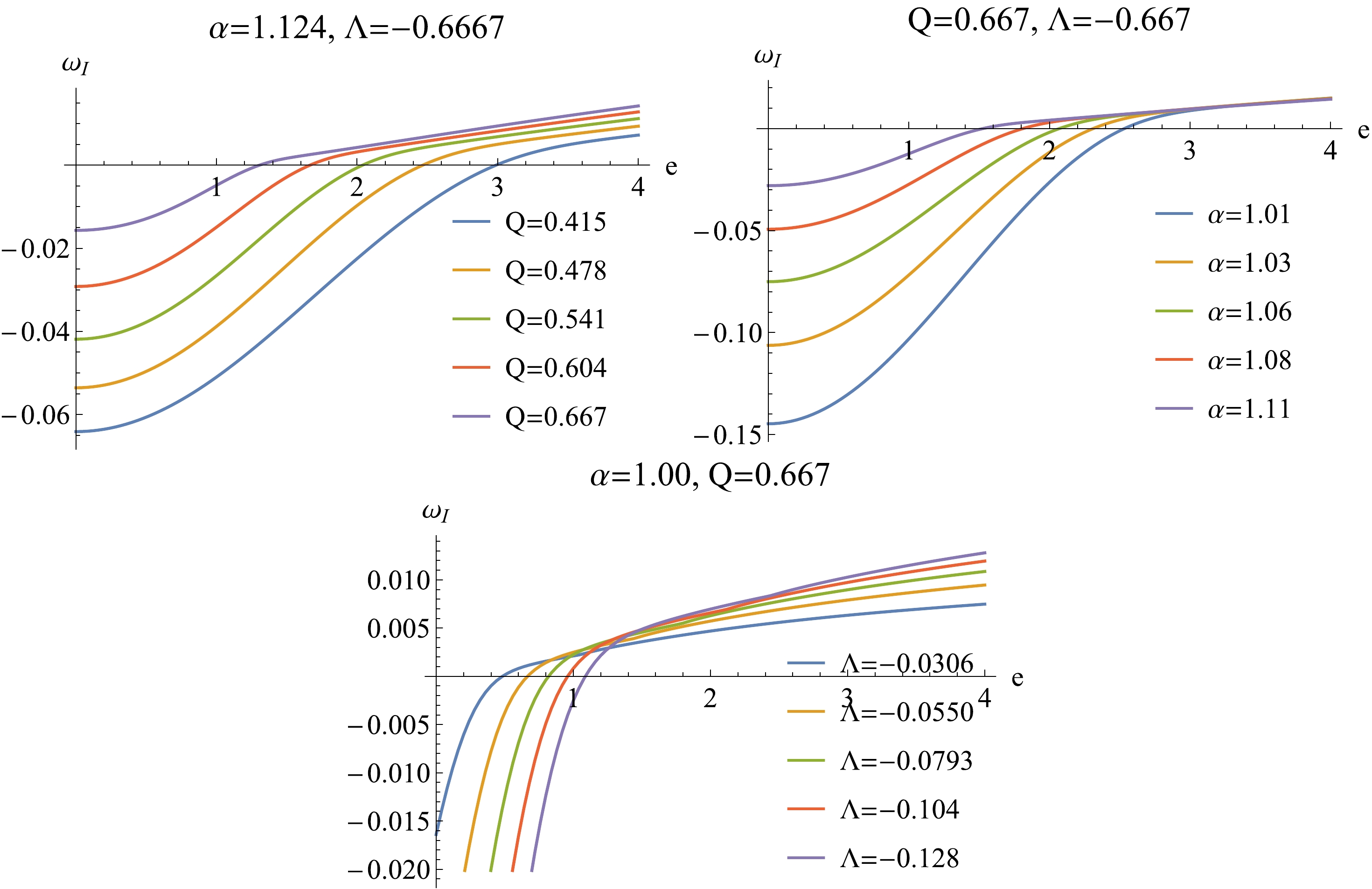
Figure 9. (color online) From top to bottom, the QNMs vs e at several different values of
$ Q,\,\alpha,\,\Lambda $ , respectively. -
In order to determine the linear instability structure, we need to locate the critical surfaces on which
$ \omega_I $ vanishes. By searching the parameter space subject to the allowed region, we show a comprehensive stable region in Fig. 10 when$ e = 1,\,l = 0 $ . The linear instability structure in parameter space$ (\alpha, \, Q,\, \Lambda) $ is much simpler than that of the dS case [61]. Figure 10 suggests that the system becomes more unstable with increasing Q or$ \alpha $ , while increasing$ \Lambda $ will make the system more stable. Comparing the solid curves$ (e = 1) $ and the dashed curves$ (e = 1.263) $ in Fig. 10, we find that the stable region indeed shrinks with increasing e. This is consistent with the results from previous subsections.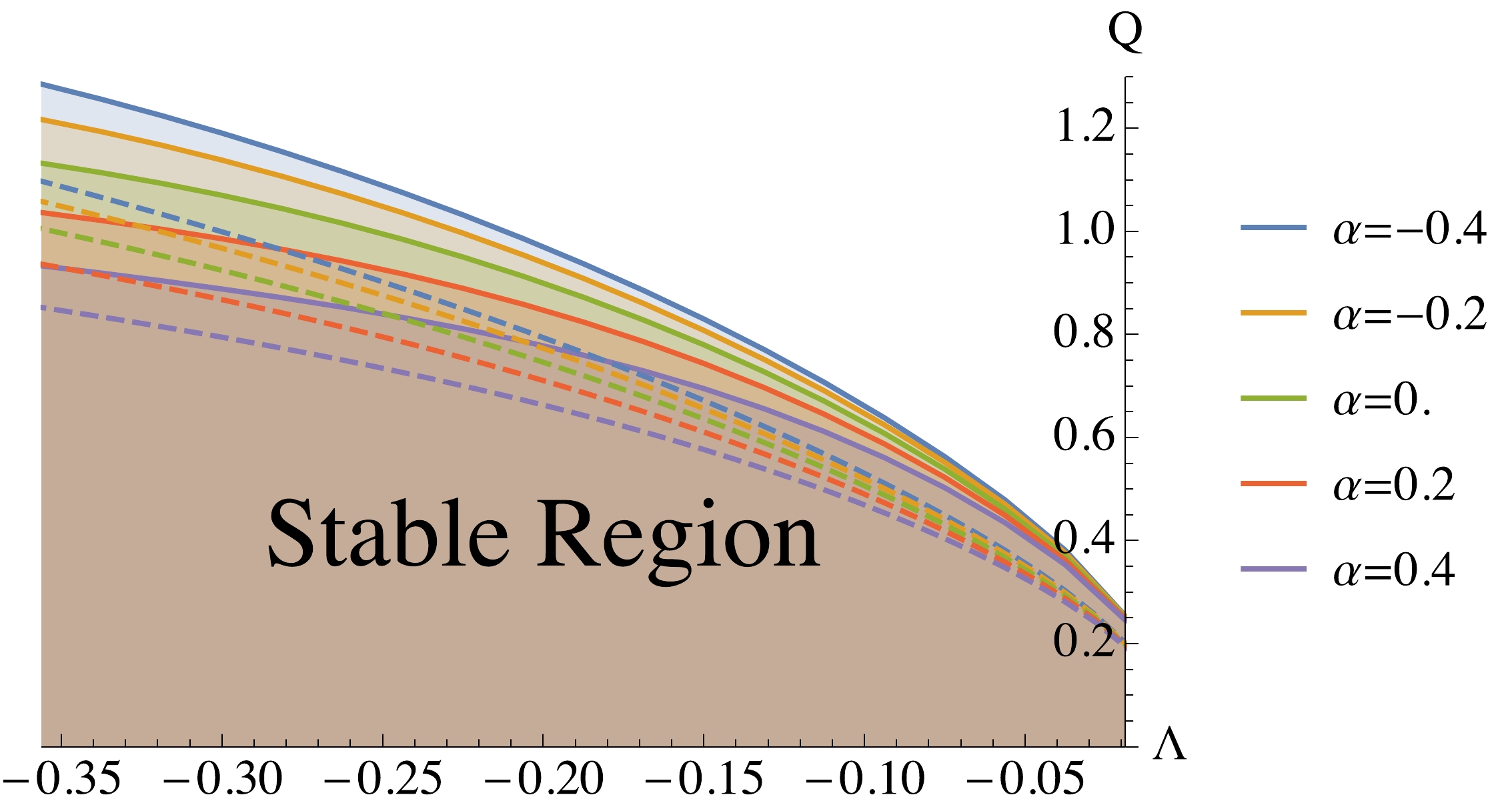
Figure 10. (color online) The shaded regions are the stable regions at
$ e = 1,\, l = 0 $ , where each solid line corresponds to different values of$ \alpha $ marked by the plot legends. The dashed lines are the critical lines for$ e = 1.263 $ , with$ \alpha $ specified by the plot legends with the same color.In the unstable region, we find that the real part of the fundamental mode frequencies of the massless charged scalar perturbation always satisfy the superradiance condition,
$ \frac{eQ}{r_+} > \omega_R. $

(20) In the stable region, the fundamental modes violate the above condition. This suggests that the linear instability from the QNM analysis is triggered by the superradiance instability. We list the QNMs at several critical points of the linear stability/instability transitions in Table 1, from which we find that
$ eQ/r_+ $ matches perfectly with the real part of the QNMs. We recall that in the dS case [61], the superradiance condition is a necessary but not sufficient condition for linear instability.$ \alpha $ 

$ \Lambda $ 

$ \dfrac{eQ}{r_+} $ 

$ \omega $ 

$ -0.4 $ 

$ -0.337501 $ 

$ {1.25639} $ 

$ {1.25639} +3.56078\times 10^{-7} i $ 

$ -0.4 $ 

$ -0.356251 $ 

$ {1.28588} $ 

$ {1.28588} +8.14388\times 10^{-8} i $ 

$ -0.2 $ 

$ -0.337501 $ 

$ {1.19356} $ 

$ {1.19355} +6.51663\times 10^{-7} i $ 

$ -0.2 $ 

$ -0.356251 $ 

$ {1.21722} $ 

$ {1.21722} +4.84345\times 10^{-7} i $ 

$ 0. $ 

$ -0.337501 $ 

$ {1.11398} $ 

$ {1.11398} -1.03083\times 10^{-6} i $ 

$ 0. $ 

$ -0.356251 $ 

$ {1.13248} $ 

$ {1.13248} +1.60832\times 10^{-7} i $ 

$ 0.2 $ 

$ -0.337501 $ 

$ {1.02122} $ 

$ {1.02122} +7.20995\times 10^{-7} i $ 

$ 0.2 $ 

$ -0.356251 $ 

$ {1.03673} $ 

$ {1.03673} -3.68094\times 10^{-7} i $ 

$ 0.4 $ 

$ -0.337501 $ 

$ {0.919189} $ 

$ {0.919191} -5.03797\times 10^{-7} i $ 

$ 0.4 $ 

$ -0.356251 $ 

$ {0.933379} $ 

$ {0.933378} +1.42506\times 10^{-7} i $ 

Table 1. Fundamental modes at several critical points of the stability-instability transitions corresponding to Fig. 10.
-
In this subsection, we directly implement the time evolution, i.e. the time integral, of the perturbation field subject to Eq. (12). This analysis is important since it can reveal the linear instability structure in a more transparent manner. It can also work as a double check of the frequency analysis.
On the event horizon, we set the ingoing boundary condition. On the AdS boundary, we set
$ \phi(v,z = 0) = 0 $ as required by the asymptotic AdS geometry. We discretize the spatial direction z with a Gauss-Lobatto collocation. In the time direction v, we use the fourth order Runge-Kutta method, which has been widely adopted in time evolution problems. Given a certain initial profile of the scalar perturbation$ \phi $ , the time evolution can be obtained.We show the time evolution of
$ \phi $ near critical lines in Fig. 11, where we can see that$ \log |\phi| $ quickly becomes linear with t. It seems like all the curves are flat, but they have very small slopes, as can be seen from Table 1. The small slope (either positive or negative) is expected since the system is near the critical line for the linear stability/instability transition.
Figure 11. (color online) Time integral of the perturbation
$ \phi(z = 0.997,v) $ at different values of$ \alpha, \Lambda, Q $ in the critical region. The initial profile of$ \phi $ is$ \phi(z,v = 0) = {\rm e}^{-5{(z-0.5)^2}} $ . The time step is$ \Delta v = 0.0025 $ , and we evolve the perturbation to$ v = 200 $ .We calculated
$ \partial_t \log |\phi| $ at$ t = 1000 $ , which is large enough to obtain stable slopes, i.e., the imaginary part of the dominant modes. The slopes should match the results from the frequency analysis. In our numerical calculation we find that they do indeed match well. For example, the slope for$ \alpha = -0.2000, \Lambda = -0.3375, Q = 1.194 $ is$ 6.50994\times 10^{-7} $ , where$ \omega_I = 6.51663\times 10^{-7} $ , as we can see from the third row in Table 1. These are results near the critical lines, where the numerical precision is hard to control since$ \omega_I $ tends to vanish in critical regions. For regions away from the critical region, the time integral results match much better with those of the frequency analysis. We show some examples in Fig. 12. For the unstable modes, the slopes are positive, while for stable modes, the slopes are negative. The stabilized slopes do not depend on the specific initial profiles and the locations where we sample the scalar perturbations$ \phi $ . The above results show that our frequency analysis is robust.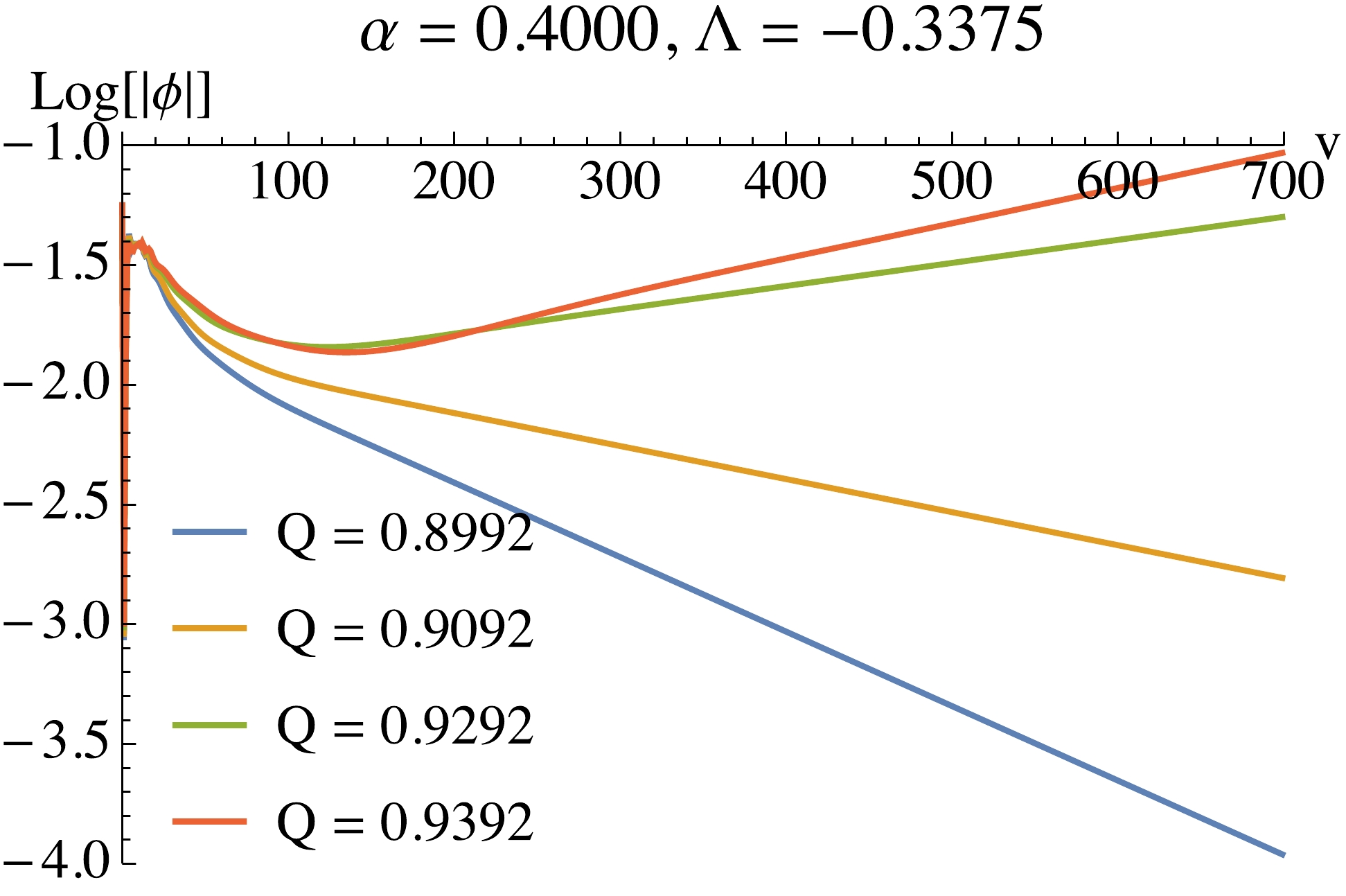
Figure 12. (color online) Time integral of the perturbation
$ \phi(z = 0.997,v) $ at different values of$ \alpha, \Lambda, Q $ away from the critical region. The initial profile of$ \phi $ is$ \phi(z,v = 0) = {\rm e}^{-5{(z-0.5)^2}} $ . The time step is$ \Delta v = 0.01 $ , and we evolve the perturbation to$ v = 700 $ . -
We have studied the linear instability of the charged massless scalar field in a regularized 4D charged EGB model with asymptotic AdS boundary by examining the QNMs. The detailed linear instability structure of the model was studied by examining the QNMs as functions of the system parameters
$ (\alpha, \, Q,\, \Lambda) $ and the scalar charge e. We find that the system is unstable against the charged massless scalar with increasing$ \alpha $ and Q, or increasing$ \Lambda $ . These phenomena have been explained intuitively from the viewpoint of the effective potential. Also, we find that the system is more unstable for larger perturbation charge e and smaller values of l. Moreover, the superradiance condition starts to be satisfied across the critical line where linear instability occurs. The time evolution of the perturbation field matches perfectly with the results from the frequency analysis.Finally, we point out several topics worthy of further study. First, it would be interesting to explore the linear instability structure of the present theory with a massive perturbation. In addition to the scalar perturbation, it is also desirable to reveal the linear instability for tensor perturbations and Dirac fields. Moreover, the instability of the background metric is also worthy of further study.
-
We thank Peng-Cheng Li, Minyong Guo for helpful discussions. Peng Liu would like to thank Yun-Ha Zha for her kind encouragement during this work.
Linear instability of charged massless scalar perturbation in regularized 4D charged Einstein-Gauss-Bonnet anti de-Sitter black holes
- Received Date: 2020-10-09
- Available Online: 2021-02-15
Abstract: We study the linear instability of the charged massless scalar perturbation in regularized 4D charged Einstein-Gauss-Bonnet-AdS black holes by exploring their quasinormal modes. We find that the linear instability is triggered by superradiance. The charged massless scalar perturbation becomes more unstable with increasing Gauss-Bonnet coupling constant or black hole charge. Decreasing the AdS radius, on the other hand, will make the charged massless scalar perturbation more stable. The stable region in parameter space (α, Q, Λ) is given. Moreover, we find that the charged massless scalar perturbation is more unstable for larger scalar charge. The modes of multipoles are more stable than that of the monopole.


 DownLoad: