


 Abstract
 HTML
HTML Reference
 Related
 PDF
PDF


-
The strangeonium (
$ s\bar{s} $ ) states, one of the types of quarkonium state predicted in the quark model, lie between the light$ q\bar{q} $ states and heavy charmonium ($ c\bar{c} $ ) states. The$ s\bar{s} $ states provide a bridge for systematically exploring quantum chromodynamics (QCD) for light and heavy quarks. Furthermore, the study of$ s\bar{s} $ states is associated with the related topic of non-$ q\bar{q} $ states (glueballs, hybrids, and tetraquarks etc.) with the same quantum numbers as conventional$ q\bar{q} $ systems [1]. To confirm a non-$ q\bar{q} $ state from experiments, one needs good knowledge of the conventional$ q\bar{q} $ states. However, at present data for the$ s\bar{s} $ spectrum are rather scarce [1, 2]. There are only a few experimentally well established resonances,$ \phi(1020) $ ,$ \phi(1680) $ ,$ h_1(1415) $ ,$ f_2'(1525) $ and$ \phi_{3}(1850) $ , which are widely accepted as$ s\bar{s} $ states. Besides some low-lying$ 1P $ - and$ 1D $ -wave states, many$ s\bar{s} $ states predicted in the quark model have yet to be established. For a long time, information on the$ s\bar{s} $ states was mainly extracted from the$ \gamma p $ ,$ K^-p $ ,$ \pi^-p $ , and$ e^+e^- $ reactions. The lack of data may be due to the fact that these experiments do not efficiently produce$ s\bar{s} $ states.The BESIII experiment provides a powerful platform for the study of
$ s\bar{s} $ states, with the world's largest$ J/\psi $ and$ \psi(2S) $ samples, which are well suited to study the$ s\bar{s} $ spectrum via their decays [2-4]. Recently, the BESIII Collaboration not only confirmed many$ s\bar{s} $ candidates observed in previous experiments, but also found some new$ s\bar{s} $ candidates by the decays of$ J/\psi $ and$ \psi(2S) $ . For example, in 2019, evidence of a new$ 1^{+} $ resonance$ X(2060) $ with a mass of$ M = (2062.8\pm13.1\pm7.2) $ MeV [or$ 1^{-} $ resonance$ X(2000) $ with$ M = (2002.1\pm27.5\pm15.0) $ MeV] was observed in$ J/\psi\to \phi \eta \eta' $ at BESIII [5]. This resonance may be a candidate for the$ 2^1P_1 $ (or$ 3^3S_1 $ [6])$ s\bar{s} $ state. In 2018, by an amplitude analysis of the process$ J/\psi\to \gamma K_SK_S $ , several isoscalar$ 0^{++} $ and$ 2^{++} $ states around$ 1.3-2.5 $ GeV were extracted with a high significance by the BEIII Collaboration; the broad$ 0^{++} $ state, with a mass of$ M = (2411\pm17) $ MeV, and the broad$ 2^{++} $ state, with a mass of$ M = (2233\pm 34 $ $ ^{+9}_{-25}) $ MeV, might be candidates for the$ 3^3P_0 $ and$ 1^3F_2 $ $ s\bar{s} $ states, respectively [7]. In 2016, several isoscalar$ 0^{-+} $ ,$ 0^{++} $ and$ 2^{++} $ states around$ 2.0-2.4 $ GeV were observed in$ J/\psi\to \gamma \phi\phi $ at BESIII [8]. The$ f_2(2010) $ confirmed in this process might be a candidate for the$ 2^3P_2 $ $ s\bar{s} $ state, while the newly observed resonance$ X(2500) $ might be a candidate for a higher$ 0^{-+} $ $ s\bar{s} $ state [9]. The world's most precise resonance parameters for$ h_1(1415) $ were also determined by a recent measurement of$ J/\psi \to \eta' K\bar{K}\pi $ at BESIII [10]. Recently, the vector meson resonance$ \phi(2170) $ (often denoted$ Y (2175) $ in the literature) was also confirmed in the$ K^+(1460)K^- $ ,$ K^+_1(1400)K^- $ ,$ K^+_1(1270)K^- $ , and$ \phi\eta' $ final states by the BESIII Collaboration [11, 12]. This state might be a candidate for the$ 3^3S_1 $ or$ 2^3D_1 $ $ s\bar{s} $ state [6, 13-16]. It should be mentioned that some forthcoming experiments from other collaborations, including COMPASS, BelleII, GlueX, and PANDA, will also provide more opportunities to study the$ s\bar{s} $ states.Theoretically, the
$ s\bar{s} $ mass spectrum has been widely discussed within various quark models, including the relativized quark model [17, 18], the nonrelativistic covariant oscillator quark model [19], the QCD-motivated relativistic quark model [20], the nonrelativistic constituent quark model constrained in the study of the$ NN $ phenomenology and the baryon spectrum [21], the nonrelativistic constituent quark potential model [22], the extended Nambu-Jona-Lasinio quark model [23, 24], the Regge trajectory approach [15, 25], the modified relativized quark model [6], the framework of the Bethe-Salpeter equation [26-28], and so on. Furthermore, the strong decay properties of strangeonia have been studied within the pseudoscalar emission model [17], the flux-tube breaking model [29, 30], the$ ^3P_0 $ model [16], the corrected$ ^3P_0 $ model [31], the relativistic quark model framework [26], and so on. However, a systematic study of both the$ s\bar{s} $ mass spectrum and their decays by combining recent experimental progress is not found in the literature. An early review of the status of the$ s\bar{s} $ spectrum can be found in Ref. [32].Stimulated by recent notable progress in experiments, we carry out a systematic study of both the mass spectrum and strong decay properties of the
$ s\bar{s} $ system. First, we calculate the mass spectrum up to the mass region of$ 3D $ -wave states within a nonrelativistic constituent quark potential model by partially adopting the model parameters determined by the$ \Omega $ spectrum [33]. As done in the literature, e.g. Refs. [34-36], the spin-dependent potentials are dealt with non-perturbatively so that the effects of the spin-dependent interactions on the wave-functions can be included. More importantly, with the widely used$ ^3P_0 $ model [37-39] we further analyze the Okubo-Zweig-Iizuka (OZI)-allowed two-body strong decays of the$ s\bar{s} $ states by using wave functions obtained from the potential model, which are crucial to identify the nature of the resonances observed in experiments. We obtain successful explanations of both the mass and strong decay properties for the well established states$ \phi(1020) $ ,$ \phi(1680) $ ,$ h_1(1415) $ ,$ f'_2(1525) $ , and$ \phi_3(1850) $ . We find that (i) the$ f_2(2010) $ and$ f_2(2150) $ listed by the Particle Data Group (PDG) [1] might be candidates for the$ 2^3P_2 $ and$ 1^3F_2 $ $ s\bar{s} $ states, respectively; (ii) the$ 4^{++} $ resonance$ f_4(2210) $ first observed in the reaction$ K^-p\to K^+K^- \Lambda $ by the LASS Collaboration [40] might be an assignment of the$ 1^3F_4 $ $ s\bar{s} $ state; (iii) the$ f_0(2410) $ observed in$ J/\psi\to K_SK_S $ at BESIII [7] may favor the assignment of the$ 3^3P_0 $ $ s\bar{s} $ state; (iv) the newly observed resonances$ X(2500) $ [8] and$ X(2062) $ [5] from BESIII may be identified as the$ 4^1S_0 $ and$ 2^1P_1 $ $ s\bar{s} $ states, respectively; and (v) the possibility of$ \phi(2170) $ as a candidate for$ \phi(3S) $ or$ \phi(2D) $ cannot be excluded, as the strong decay properties are very sensitive to its mass.This paper is organized as follows. In Sec. II, the mass spectrum is calculated within a nonrelativistic linear potential model. Then, by using the obtained spectrum the OZI-allowed two-body strong decays of the
$ s\bar{s} $ states are estimated in Sec. III within the$ ^3P_0 $ model. In Sec. IV, we discuss the properties of the$ s\bar{s} $ states by combining our predictions with the experimental observations or other model predictions. Finally, a summary is given in Sec. V. -
To calculate the
$ s\bar{s} $ mass spectrum, we adopt a nonrelativistic potential model [34-36, 41, 42]. In this model, the effective quark-antiquark potential is written as the sum of the spin-independent term$ H_0(r) $ and spin-dependent term$ H_{\rm sd}(r) $ :$ V(r) = H_0(r)+H_{\rm sd}(r), $

(1) where
$ H_0(r) = -\frac{4}{3}\frac{\alpha_s}{r}+br+C_{0} $

(2) includes the standard color Coulomb interaction and the linear confinement. The spin-dependent part
$ H_{\rm sd}(r) $ can be expressed as [43]:$ H_{\rm sd}(r) = H_{SS}+H_{T}+H_{LS}, $

(3) where
$ H_{SS} = \frac{32\pi\alpha_s}{9m_qm_{\bar{q}}}\tilde{\delta}_\sigma(r){\bf{S}}_{q}\cdot {\bf{S}}_{\bar{q}} $

(4) is the spin-spin contact hyperfine potential. Here, we take
$ \tilde{\delta}_\sigma(r) = (\sigma/\sqrt{\pi})^3 {\rm e}^{-\sigma^2r^2} $ , as suggested in Ref. [41]. The tensor potential$ H_T $ is:$ H_{T} = \frac{4}{3}\frac{\alpha_s}{m_qm_{\bar{q}}}\frac{1}{r^3}\left(\frac{3{{S}}_{q}\cdot {{r}}{{S}}_{\bar{q}}\cdot {{r}}}{r^2}-{{S}}_{q}\cdot{{S}}_{\bar{q}}\right). $

(5) For convenience in the calculations, the potential of the spin-orbit interaction
$ H_{LS} $ is decomposed into a symmetric part$ H_{\rm sym} $ and antisymmetric part$ H_{\rm anti} $ ,$ H_{LS} = H_{\rm sym}+H_{\rm anti}, $

(6) with
$ H_{\rm sym} = \frac{{ S}_{+}\cdot {{L}}}{2}\left[\left(\frac{1}{2m_{\bar{q}}^{2}}+\frac{1}{2m_{q}^{2}}\right)\left(\frac{4}{3}\frac{\alpha_{s}}{r^{3}}-\frac{b}{r}\right) +\frac{8\alpha_{s}}{3m_{q}m_{\bar{q}}r^{3}}\right], $

(7) $ H_{\rm anti} = \frac{{ S}_{-}\cdot {{L}}}{2}\left(\frac{1}{2m_{q}^{2}}-\frac{1}{2m_{\bar{q}}^{2}}\right)\left(\frac{4}{3}\frac{\alpha_{s}}{r^{3}}-\frac{b}{r}\right). $

(8) In these equations,
$ {{L}} $ is the relative orbital angular momentum of the$ q\bar{q} $ system;$ {{S}}_q $ and$ {{S}}_{\bar{q}} $ are the spins of the quark q and antiquark$ \bar{q} $ , respectively, and$ {{S}}_{\pm}\equiv{{S}}_q\pm {{S}}_{\bar{q}} $ ;$ m_q $ and$ m_{\bar{q}} $ are the masses of the quark q and antiquark$ \bar{q} $ , respectively;$ \alpha_s $ is the running coupling constant of QCD; r is the distance between the quark q and antiquark$ \bar{q} $ ; and the constant$ C_0 $ is the zero point energy. The six parameters in the above equations ($ \alpha_s $ , b,$ \sigma $ ,$ m_q $ ,$ m_{\bar{q}} $ $ C_0 $ ) are determined by fitting the spectrum.Recently, the nonrelativistic potential model has been applied to study the
$ \Omega $ baryon spectrum [33]. In order to be consistent with the$ \Omega $ spectrum, we set the parameters$ \alpha_s $ ,$ \sigma $ and$ m_s $ to the same values as those determinations in Ref. [33]. The studies in Refs. [17, 44] show that the parameters b and$ C_0 $ for a$ q\bar{q} $ system might be slightly different from the$ qqq $ system, so in the present work we reasonably adjust b and$ C_0 $ to better describe the masses of$ s\bar{s} $ states$ \phi(1020) $ ,$ \phi(1680) $ and$ \phi_{3}(1850) $ . Our parameters are listed in Table 1, where they are compared to those of the$ \Omega $ baryon spectrum.This work Ref. [33] $ m_s $ /GeV

0.600 Same $ \alpha_s $ 

0.770 Same $ \sigma $ /GeV

0.600 Same b/GeV $ ^2 $ 

0.135 0.110 $ C_0 $ /GeV

$ -0.519 $ 

$ -0.694 $ 

Table 1. Parameters of the nonrelativistic potential model.
We solve the Schrödinger equation by using the three-point difference central method [45] from the centre (
$ r = 0 $ ) to the outside ($ r\to \infty $ ), point by point. This method has been successfully applied to the$ b\bar{b} $ ,$ \bar{b}c $ and$ c\bar{c} $ systems [34-36]. To overcome the singular behavior of$ 1/r^3 $ in the spin-dependent potentials, we introduce a cutoff distance$ r_{c} $ in the calculation. In a small range$ r\in(0,r_{c}) $ , we let$ 1/r^3 = 1/r_c^3 $ . With this treatment, one can deal with spin-dependent potentials nonperturbatively, so that the effects of the spin-dependent potentials on the wave-functions can be included. Considering the fact that the mass of$ 1^3D_1 $ is sensitive to the cutoff distance$ r_c $ , the mass of$ 1^3D_1 $ is used to determine the value of$ r_c $ . It should be pointed out that the$ 1^3D_1 $ state has still not been established experimentally. Thus, we adopt a theoretical mass of$ 1^3D_1 $ predicted with a perturbation method, i.e., we let$ H = H_{0}+H' $ , where$ H' $ is a part which contains the$ 1/r^{3} $ term. With the perturbation method one can obtain a fairly accurate mass, although one cannot include the effects of the spin-dependent interactions on the wave-functions. By solving the equation$ H_{0}|\psi_{n}^{(0)}\rangle = E_{0}|\psi_{n}^{(0)}\rangle $ , we get the energy$ E_{0} $ and wave function$ |\psi_{n}^{(0)}\rangle $ . Then, the mass of$ 1^3D_1 $ , 1809 MeV, is worked out with$ M = 2m_s+E_{0}+ \langle\psi_{n}^{(0)}|H'|\psi_{n}^{(0)}\rangle $ . Finally, with this predicted mass the cutoff distance$ r_c $ is determined to be$ 0.546 $ fm.Our predicted
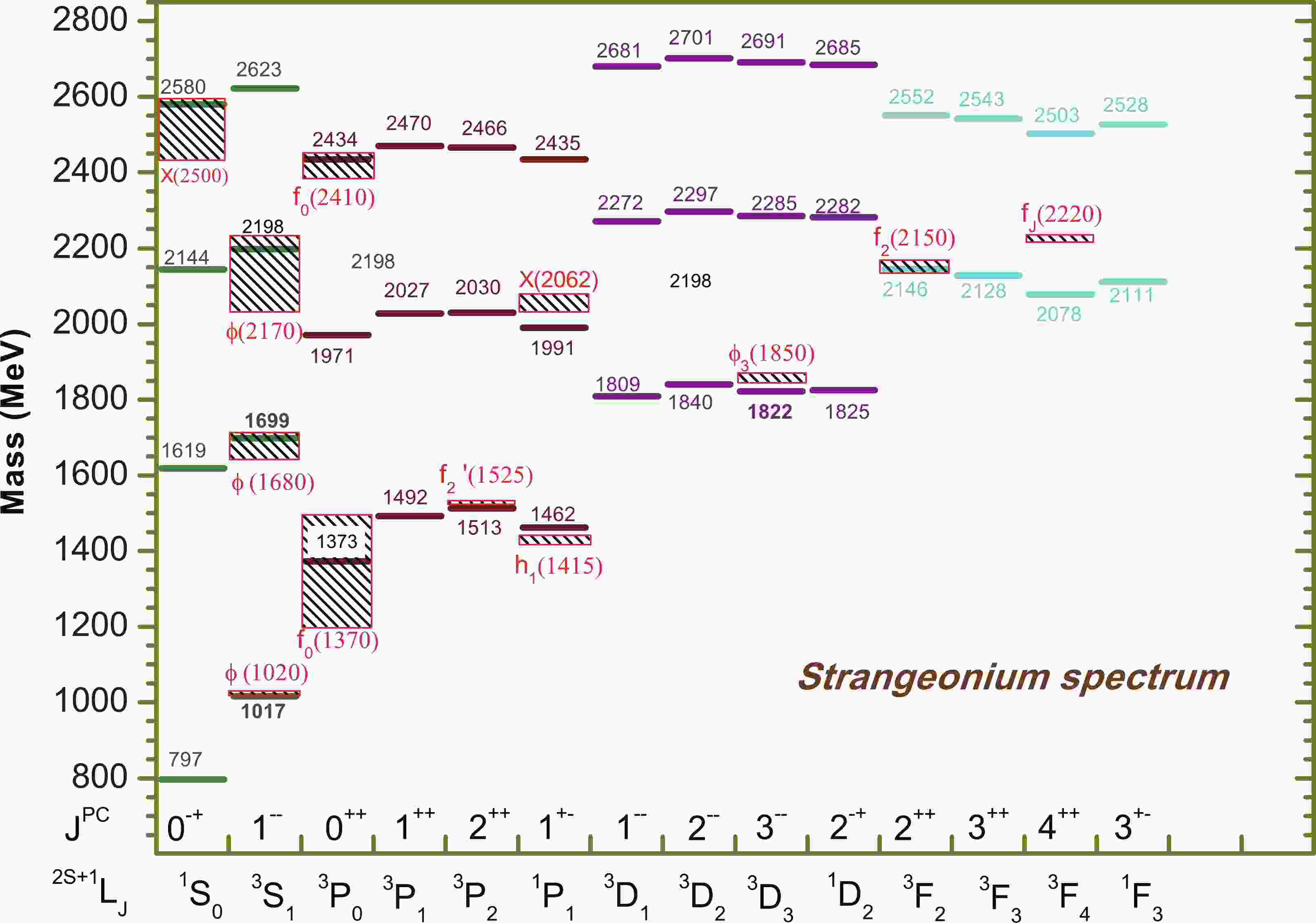
$ s\bar{s} $ mass spectrum is shown in Fig. 1. For comparison, our results together with some other model predictions and measurements are also listed in Table 2. From the table, one can see that our predictions with the nonrelativistic potential model are in reasonable agreement with the predictions of the relativized quark model [6, 17, 18], relativistic quark models [20], and nonrelativistic quark models [19, 21], although some model dependencies exist in the predictions for the higher excitations with$ n\geqslant 3 $ . To understand why acceptable results can be provided by relativistic as well as by nonrelativistic approaches, there have been some studies of the connections between relativistic, semirelativistic, and nonrelativistic potential models of quarkonium using an interaction composed of an attractive Coulomb potential and a confining power-law term [46].
$n^{2S+1}L_{J}$ 

$J^{PC}$ 

Ours XWZZ [18] EFG [20] SIKY [19] GI [17] Pang [6] VFV [21] Observed state [1] $1 ^3S_{1}$ 

$1^{–}$ 

1017 1009 1038 1020 1020 1030 1020 $\phi(1020)$ 

$1 ^1S_{0}$ 

$0^{-+}$ 

797 657 743 690 960 $\cdots$ 

956 $\cdots$ 

$2 ^3S_{1}$ 

$1^{–}$ 

1699 1688 1698 1740 1690 1687 1726 $\phi(1680)$ 

$2 ^1S_{0}$ 

$0^{-+}$ 

1619 1578 1536 1440 1630 $\cdots$ 

1795 $\cdots$ 

$3 ^3S_{1}$ 

$1^{–}$ 

2198 2204 2119 2250 $\cdots$ 

2149 $\cdots$ 

$\cdots$ 

$3 ^1S_{0}$ 

$0^{-+}$ 

2144 2125 2085 1970 $\cdots$ 

$\cdots$ 

$\cdots$ 

$\cdots$ 

$4 ^3S_{1}$ 

$1^{–}$ 

2623 2627 2472 2540 $\cdots$ 

2498 $\cdots$ 

$\cdots$ 

$4 ^1S_{0}$ 

$0^{-+}$ 

2580 2568 2439 2260 $\cdots$ 

$\cdots$ 

$\cdots$ 

$X(2500)$ [8]

$1 ^3P_{2}$ 

$2^{++}$ 

1513 1539 1529 1480 1530 $\cdots$ 

1556 $f_2'(1525)$ 

$1 ^3P_{1}$ 

$1^{++}$ 

1492 1480 1464 1430 1480 $\cdots$ 

1508 $f_1(1420)?$ 

$1 ^3P_{0}$ 

$0^{++}$ 

1373 1355 1420 1180 1360 $\cdots$ 

$\cdots$ 

$f_0(1370)$ 

$1 ^1P_{1}$ 

$1^{+-}$ 

1462 1473 1485 1460 1470 $\cdots$ 

1511 $h_1(1415)$ 

$2 ^3P_{2}$ 

$2^{++}$ 

2030 2046 2030 2080 2040 $\cdots$ 

1999 $f_2(2010)$ 

$2 ^3P_{1}$ 

$1^{++}$ 

2027 2027 2016 2020 2030 $\cdots$ 

$\cdots$ 

$\cdots$ 

$2 ^3P_{0}$ 

$0^{++}$ 

1971 1986 1969 1800 1990 $\cdots$ 

$\cdots$ 

$\cdots$ 

$2 ^1P_{1}$ 

$1^{+-}$ 

1991 2008 2024 2040 2010 $\cdots$ 

1973 $X(2062)$ [5]

$3 ^3P_{2}$ 

$2^{++}$ 

2466 2480 2412 2540 $\cdots$ 

$\cdots$ 

$\cdots$ 

$\cdots$ 

$3 ^3P_{1}$ 

$1^{++}$ 

2470 2468 2403 2480 $\cdots$ 

$\cdots$ 

$\cdots$ 

$\cdots$ 

$3 ^3P_{0}$ 

$0^{++}$ 

2434 2444 2364 2280 $\cdots$ 

$\cdots$ 

$\cdots$ 

$f_0(2410)$ [7]

$3 ^1P_{1}$ 

$1^{+-}$ 

2435 2449 2398 2490 $\cdots$ 

$\cdots$ 

$\cdots$ 

$\cdots$ 

$1 ^3D_{3}$ 

$3^{–}$ 

1822 1897 1950 1830 1900 $\cdots$ 

1875 $\phi_3(1850)$ 

$1 ^3D_{2}$ 

$2^{–}$ 

1840 1904 1908 1810 1910 $\cdots$ 

$\cdots$ 

$\cdots$ 

$1 ^3D_{1}$ 

$1^{–}$ 

1809 1883 1845 1750 1880 1869 $\cdots$ 

$\cdots$ 

$1 ^1D_{2}$ 

$2^{-+}$ 

1825 1893 1909 1830 1890 $\cdots$ 

1853 $\cdots$ 

$2 ^3D_{3}$ 

$3^{–}$ 

2285 2337 2338 2360 $\cdots$ 

$\cdots$ 

$\cdots$ 

$\cdots$ 

$2 ^3D_{2}$ 

$2^{–}$ 

2297 2348 2323 2330 $\cdots$ 

$\cdots$ 

$\cdots$ 

$\cdots$ 

$2 ^3D_{1}$ 

$1^{–}$ 

2272 2342 2258 2260 $\cdots$ 

2276 $\cdots$ 

$\cdots$ 

$2 ^1D_{2}$ 

$2^{-+}$ 

2282 2336 2321 2340 $\cdots$ 

$\cdots$ 

$\cdots$ 

$\cdots$ 

$3 ^3D_{3}$ 

$3^{–}$ 

2691 2725 2727 $\cdots$ 

$\cdots$ 

$\cdots$ 

$\cdots$ 

$\cdots$ 

$3 ^3D_{2}$ 

$2^{–}$ 

2701 2734 2667 $\cdots$ 

$\cdots$ 

$\cdots$ 

$\cdots$ 

$\cdots$ 

$3 ^3D_{1}$ 

$1^{–}$ 

2681 2732 2607 $\cdots$ 

$\cdots$ 

2593 $\cdots$ 

$\cdots$ 

$3 ^1D_{2}$ 

$2^{-+}$ 

2685 2723 2662 $\cdots$ 

$\cdots$ 

$\cdots$ 

$\cdots$ 

$\cdots$ 

$1 ^3F_{4}$ 

$4^{++}$ 

2078 2202 2286 2130 2200 $\cdots$ 

$\cdots$ 

$f_4(2210)$ [40]

$1 ^3F_{3}$ 

$3^{++}$ 

2128 2234 2215 2120 2230 $\cdots$ 

$\cdots$ 

$\cdots$ 

$1 ^3F_{2}$ 

$2^{++}$ 

2146 2243 2143 2090 2240 $\cdots$ 

$\cdots$ 

$f_2(2150)$ 

$1 ^1F_{3}$ 

$3^{+-}$ 

2111 2223 2209 2130 2220 $\cdots$ 

$\cdots$ 

$\cdots$ 

$2 ^3F_{4}$ 

$4^{++}$ 

2503 2596 2657 $\cdots$ 

$\cdots$ 

$\cdots$ 

$\cdots$ 

$\cdots$ 

$2 ^3F_{3}$ 

$3^{++}$ 

2543 2623 2585 $\cdots$ 

$\cdots$ 

$\cdots$ 

$\cdots$ 

$\cdots$ 

$2 ^3F_{2}$ 

$2^{++}$ 

2552 2636 2514 $\cdots$ 

$\cdots$ 

$\cdots$ 

$\cdots$ 

$\cdots$ 

$2 ^1F_{3}$ 

$3^{+-}$ 

2528 2613 2577 $\cdots$ 

$\cdots$ 

$\cdots$ 

$\cdots$ 

$\cdots$ 

Table 2. Predicted masses of the
$s\bar{s}$ states in this work compared with other predictions and observations. -
In this work the Okubo-Zweig-Iizuka (OZI)-allowed two-body strong decays of the
$ s\bar{s} $ states are calculated with the widely used$ ^{3}P_0 $ model [37-39]. In this model, one assumes that a quark-antiquark pair is produced from the vacuum with the quantum number$ 0^{++} $ and the initial meson decay takes place via the rearrangement of the four quarks as shown in Fig. 2. In the nonrelativistic limit, the transition operator is expressed as: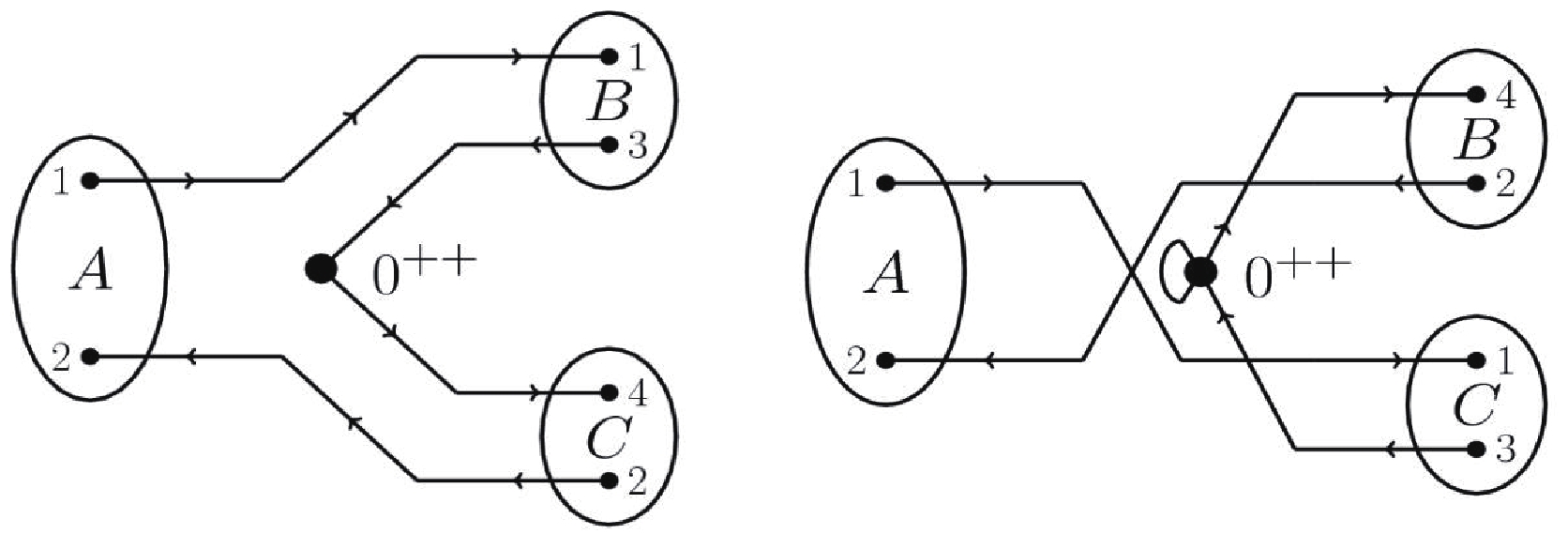
Figure 2. The meson two-body strong decay process
$ A \to BC $ in the$ ^3P_0 $ model.$\begin{aligned}[b] \hat{T} =& -3 \gamma \sqrt{96 \pi} \sum_{m}^{} \langle 1 m 1 -m| 0 0 \rangle \int_{}^{} {\rm d}{{p}}_3 {\rm d}{{p}}_4 \delta^3 ({{p}}_3 + {{p}}_4) \\ & \times {\cal{Y}}_1^m \left(\frac{{{p}}_3 - {{p}}_4}{2}\right) \chi_{1-m}^{34} \phi_0^{34} \omega_0^{34} b_{3i}^\dagger ({{p}}_3) d_{4j}^\dagger ({{p}}_4) \ , \end{aligned}$

(9) where
$ \gamma $ is a dimensionless constant that denotes the strength of the quark-antiquark pair creation with momenta$ {{p}}_3 $ and$ {{p}}_4 $ from vacuum;$ b_{3i}^\dagger ({{p}}_3) $ and$ d_{4j}^\dagger({{p}}_4) $ are the creation operators for the quark and antiquark, respectively; the subscripts i and j are the SU(3)-color indices of the created quark and antiquark;$ \phi_0^{34} = (u\bar u + d\bar d +s \bar s)/\sqrt 3 $ and$ \omega_{0}^{34} = \dfrac{1}{\sqrt{3}} \delta_{ij} $ correspond to flavor and color singlets, respectively;$ \chi_{{1,-m}}^{34} $ is a spin triplet state; and$ {\cal{Y}}_{\ell m}({{k}})\equiv |{{k}}|^{\ell}Y_{\ell m}(\theta_{{{k}}},\phi_{{{k}}}) $ is the$ \ell $ -th solid harmonic polynomial.For an OZI-allowed two-body strong decay process
$ A\to B+C $ , the helicity amplitude$ {\cal{M}}^{M_{J_A}M_{J_B} M_{J_C}}({{P}}) $ can be worked out by:$ \langle BC|T| A\rangle = \delta({{P}}_A-{{P}}_B-{{P}}_C){\cal{M}}^{M_{J_A}M_{J_B} M_{J_C}}({{P}}). $

(10) In the center-of-mass (c.m.) frame of the initial meson A, the helicity amplitude can be written as:
$ \begin{aligned}[b] {\cal{M}}^{M_{J_A}M_{J_B} M_{J_C}}({{P}}) =& \gamma \sqrt{96 \pi} \sum_{\begin{subarray}{l} M_{L_A},M_{S_A}, M_{L_B},M_{S_B}, M_{L_C},M_{S_C},m \end{subarray}} \langle L_A M_{L_A}; S_A M_{S_A} | J_A M_{J_A} \rangle \times \langle 1\;m;1\;-m|\;0\;0 \rangle\langle L_B M_{L_B}; S_B M_{S_B} | J_B M_{J_B} \rangle \\& \times\langle L_C M_{L_C}; S_C M_{S_C} | J_C M_{J_C} \rangle\times \langle \chi^{1 3}_{S_B M_{S_B}}\chi^{2 4}_{S_CM_{S_C}} | \chi^{1 2}_{S_A M_{S_A}} \chi^{3 4}_{1 -\!m} \rangle\\ & \times[\langle\phi^{13}_B \phi^{2 4}_C | \phi^{1 2}_A \phi^{3 4}_0\rangle I^{M_{L_A},m}_{M_{L_B},M_{L_C}}({{P}}) +(-1)^{S_A+S_B+S_C+1}\langle\phi^{2 4}_B \phi^{1 3}_C | \phi^{1 2}_A \phi^{3 4}_0\rangle I^{M_{L_A},m}_{M_{L_B},M_{L_C}}({-P)}], \end{aligned}$

(11) with the integral in momentum space:
$ \begin{aligned}[b] I^{M_{L_A},m}_{M_{L_B},M_{L_C}}({{P}}) =& \int {\rm d}^3{{p}}_3 \Psi^*_{n_B L_B M_{L_B}}\left(\frac{m_3 {{P}}}{m_1+m_3}-{{p}}_3 \right){\cal{Y}}_{1m}({{p}}_3)\\& \times\Psi^*_{n_C L_C M_{L_C}}\left(\frac{-m_3 {{P}}}{m_2+m_3}+{{p}}_3 \right)\Psi_{n_A L_A M_{L_A}}\left({{P}}-{{p}}_3 \right). \end{aligned}$

(12) In the above equations, (
$ J_{A} $ ,$ J_{B} $ and$ J_{C} $ ), ($ L_A $ ,$ L_B $ and$ L_C $ ) and ($ S_A $ ,$ S_B $ and$ S_C $ ) are the quantum numbers of the total angular momentum, orbital angular momentum and total spin for hadrons$ A,\,B,\,C $ , respectively; in the c.m. frame of hadron A, the momenta$ {{P}}_B $ and$ {{P}}_C $ of mesons B and C satisfy$ {{P}}_B = -{{P}}_C\equiv {{P}} $ ;$ m_1 $ and$ m_2 $ are the constituent quark masses of the initial hadron A;$ m_3 $ is the mass of the anti-quark created from vacuum;$ \Psi_{n_A L_A M_{L_A}} $ ,$ \Psi_{n_B L_B M_{L_B}} $ and$ \Psi_{n_C L_C M_{L_C}} $ are the radial wave functions of hadrons A, B and C, respectively, in momentum space, while$ \phi^{12}_A $ ,$ \phi^{13}_B $ and$ \phi^{24}_C $ ($ \chi^{1 2}_{S_A M_{S_A}} $ ,$ \chi^{1 3}_{S_B M_{S_B}} $ and$ \chi^{2 4}_{S_C M_{S_C}} $ ) are the flavor (spin) wave functions of hadrons A, B and C, respectively;$ \langle \phi^{1 3}_B \phi^{2 4}_C | \phi^{1 2}_A \phi^{3 4}_{00}\rangle $ and$ \langle \chi^{1 3}_{S_B M_{S_B}} \chi^{2 4}_{S_C M_{S_C}}| \chi^{1 2}_{S_A M_{S_A}} \chi^{3 4}_{1 -\!m} \rangle $ are the flavor and spin matrix elements, respectively; and$ \langle L_A M_{L_A}; S_A M_{S_A} | J_A M_{J_A} \rangle $ and$ \langle L_B M_{L_B}; S_B M_{S_B} | J_B M_{J_B} \rangle $ ,$ \langle L_C M_{L_C}; S_C M_{S_C} | J_C M_{J_C} \rangle $ and$ \langle 1\;m;1\;-m|\;0\;0 \rangle $ are the corresponding Clebsch-Gordan coefficients.With the Jacob-Wick formula [47], the helicity amplitudes
$ {\cal{M}}^{M_{J_A}M_{J_B} M_{J_C}}({{P}}) $ can be converted to the partial wave amplitudes$ {\cal{M}}^{JL} $ via$\begin{aligned}[b] {{\cal{M}}}^{J L}(A\rightarrow BC) =& \frac{\sqrt{4\pi (2 L+1)}}{2 J_A+1} \sum_{M_{J_B},M_{J_C}} \langle L 0 J M_{J_A}|J_A M_{J_A}\rangle\\& \times \langle J_B M_{J_B} J_C M_{J_C} | J M_{J_A} \rangle {\cal{M}}^{M_{J_A} M_{J_B} M_{J_C}}({{P}}), \end{aligned}$

(13) where
$ M_{J_A} = M_{J_B}+M_{J_C} $ ,$ {{J}}\equiv {{J}}_B+{{J}}_C $ and$ {{J}}_{A} \equiv {{J}}_{B}+ {{J}}_C+{{L}} $ . More details of the$ ^3P_0 $ model can be found in our recent paper [48].To partly remedy the inadequacy of the nonrelativistic wave function as the momentum
$ {{P}} $ increases, the partial width of the$ A\to B+C $ process is calculated with a semirelativistic phase space [29, 30]:$ \Gamma = 2\pi |{{P}}| \frac{M_B M_C}{M_A}\sum_{JL}\Big |{\cal{M}}^{J L}\Big|^2, $

(14) where
$ M_A $ is the mass of the initial hadron A, while$ M_B $ and$ M_C $ stand for the masses of final hadrons B and C, respectiIn our calculation, the masses of the final hadrons B and C appearing in the phase space are given "mock" values as suggested in Ref. [29]. These are worked out by:$ \begin{aligned}[b] \tilde{M}(fnL) = &\frac{1}{4}M(fnL;S = 0,J = L)\\ & +{\sum\limits_{m = -1,0,1}\frac{2(L+m)+1}{4(2L+1)} M(fnL;S = 1,J = L+m)}, \end{aligned} $

(15) where
$ \tilde{M} $ , M, n, L, S, m stand for the mock mass, mass, principal quantum number, orbital quantum number, spin quantum number, and the third component of spin momentum, respectively. The masses and mock masses of final meson states are shown in Table 3. The masses of the initial hadrons, where known experimentally, are taken from the PDG [1]; otherwise their masses are taken from our potential model predictions as listed in Table 2.Meson $n^{2S+1}L_J$ 

$J^{P(C)}$ 

Mass/MeV $\tilde{M}$ /MeV

Flavor function $K$ 

$1 ^1S_{0}$ 

$0^{-}$ 

494 793 $K^+ = u\bar{s},\,K^- = \bar{u}s,\,K^0 = d\bar{s},\,\bar{K^0} = \bar{d}s$ 

$K^*$ 

$1 ^3S_{1}$ 

$1^{-}$ 

896 793 $K^{*+} = u\bar{s},\,K^{*-} = \bar{u}s,\,K^{*0} = d\bar{s},\,\bar{K^{*0}} = \bar{d}s$ 

$K(1460)$ 

$2 ^1S_{0}$ 

$0^{-}$ 

1460 1580 $K^+ = u\bar{s},\,K^- = \bar{u}s,\,K^0 = d\bar{s},\,\bar{K^0} = \bar{d}s$ 

$K^*(1410)$ 

$2 ^3S_{1}$ 

$1^{-}$ 

1580 1580 $K^{*+} = u\bar{s},\,K^{*-} = \bar{u}s,\,K^{*0} = d\bar{s},\,\bar{K^{*0}} = \bar{d}s$ 

$K^*_0(1430)$ 

$1 ^3P_{0}$ 

$0^{+}$ 

1425 1381 $K^{*+}_0 = u\bar{s},\,K^{*-}_0 = \bar{u}s,\,K^{*0}_0 = d\bar{s},\,\bar{K^{*0}_0} = \bar{d}s$ 

$K_1(1270)$ 

$\cos\theta_{1P}|1\;^{1}P_1\rangle +\sin\theta_{1P}|1\;^{3}P_1\rangle$ 

$1^{+}$ 

1272 1381 $K^+_1 = u\bar{s},\,K^-_1 = \bar{u}s,\,K^0_1 = d\bar{s},\,\bar{K^0_1} = \bar{d}s$ 

$K_1(1400)$ 

$ -\sin\theta_{1P}|1\;^{1}P_1\rangle +\cos\theta_{1P}|1\;^{3}P_1\rangle$ 

$1^{+}$ 

1403 1381 $K^+_1 = u\bar{s},\,K^-_1 = \bar{u}s,\,K^0_1 = d\bar{s},\,\bar{K^0_1} = \bar{d}s$ 

$\theta_{1P} = 45^\circ$ [1,49]

$K^*_2(1430)$ 

$1 ^3P_{2}$ 

$2^{+}$ 

1426 1381 $K^{*+}_2 = u\bar{s},\,K^{*-}_2 = \bar{u}s,\,K^{*0}_2 = d\bar{s},\,\bar{K^{*0}_2} = \bar{d}s$ 

$K^*(1680)$ 

$1 ^3D_{1}$ 

$1^{-}$ 

1718 1756 $K^{*+} = u\bar{s},\,K^{*-} = \bar{u}s,\,K^{*0} = d\bar{s},\,\bar{K^{*0}} = \bar{d}s$ 

$K_2(1770)$ 

$\cos\theta_{1D}|1^{1}D_2\rangle +\sin\theta_{1D}|1^{3}D_2\rangle$ 

$2^{-}$ 

1773 1756 $K^+_2 = u\bar{s},\,K^-_2 = \bar{u}s,\,K^0_2 = d\bar{s},\,\bar{K^0_2} = \bar{d}s$ 

$K_2(1820)$ 

$ -\sin\theta_{1D}|1^{1}D_2\rangle +\cos\theta_{1D}|1^{3}D_2\rangle$ 

$2^{-}$ 

1819 1756 $K^+_2 = u\bar{s},\,K^-_2 = \bar{u}s,\,K^0_2 = d\bar{s},\,\bar{K^0_2} = \bar{d}s$ 

$\theta_{1D} = 45^\circ$ [49]

$K^*_3(1780)$ 

$1 ^3D_{3}$ 

$3^{-}$ 

1776 1756 $K^{*+}_3 = u\bar{s},\,K^{*-}_3 = \bar{u}s,\,K^{*0}_3 = d\bar{s},\,\bar{K^{*0}_3} = \bar{d}s$ 

$\eta$ 

$1 ^1S_{0}$ 

$0^{-+}$ 

548 793 $\cos\theta_1(\dfrac{u\bar{u}+d\bar{d} }{\sqrt{2} })-\sin\theta_1({s\bar{s} }),\,\theta_1 = 39.3^\circ$ 

$\eta'$ 

$1 ^1S_{0}$ 

$0^{-+}$ 

958 793 $\sin\theta_1(\dfrac{u\bar{u}+d\bar{d} }{\sqrt{2} })+\cos\theta_1({s\bar{s} }),\,\theta_1 = 39.3^\circ$ 

$\phi(1020)$ 

$1 ^3S_{1}$ 

$1^{–}$ 

1020 964 $s\bar{s}$ 

$f_0(1373)$ 

$1 ^3P_{0}$ 

$0^{++}$ 

1373 1488 $s\bar{s}$ 

$f_1(1492)$ 

$1 ^3P_{1}$ 

$1^{++}$ 

1492 1488 $s\bar{s}$ 

$h_1(1415)$ 

$1 ^1P_{1}$ 

$1^{+-}$ 

1416 1488 $s\bar{s}$ 

$f_2'(1525)$ 

$1 ^3P_{2}$ 

$2^{++}$ 

1525 1488 $s\bar{s}$ 

Table 3. Masses, mock masses (denoted with
$\tilde{M}$ ) and flavor wave functions for the final meson states. The meson masses for the well established states are taken from the PDG [1]; otherwise they are taken from our theoretical estimations. The mock masses, which correspond to the calculated mass of the meson in the spin-independent$q\bar{q}$ s potential, are calculated with Eq. (15). The mixing angles$\theta_{1P} = 45^\circ$ and$\theta_{1D} = 45^\circ$ for the$1P$ - and$1D$ -wave kaon meson states are determined according to the decay properties [1, 49].In the calculations, the wave functions of the initial and final states are taken from our potential model predictions. To obtain the wave functions for the final kaon meson states, we fit the masses of the well established states K,
$ K^* $ ,$ K(1460) $ ,$ K_2(1430) $ ,$ K^*(1680) $ , and$ K_3(1780) $ . The potential model parameters for the kaon meson spectrum are determined to be$ \alpha_s = 0.885 $ ,$ b = 0.1383 $ GeV$ ^2 $ ,$ m_s = 0.6 $ GeV,$ m_u = 0.45 $ GeV,$ \sigma = 0.669 $ GeV,$ r_c = 0.59 $ fm and$ C_0 = -0.524 $ GeV. The pair creation strength$ \gamma = 0.360 $ is obtained by fitting the width of$ \phi(1680) $ from the PDG [1]. The OZI-allowed two-body strong decay properties, such as the partial decay width, total decay width, branching fraction, and partial wave amplitude, are calculated for the$ s\bar{s} $ states listed in Table 2. Our results are listed in Tables 4-19.State Mode Ours Ref. [16] Ref. [6] $ \Gamma_{\rm th} $ [

$ \Gamma_{\exp} $ ]/MeV

$ Br $ (%)

Amps. /(GeV $ ^{-1/2} $ )

$ \Gamma_{\rm th} $ /MeV

$ Br $ (%)

$ \Gamma_{\rm th} $ /MeV

$ Br $ (%)

$ 1 ^3S_{1}[1020] $ 

$ KK $ 

4.09 [3.5] 100 $ ^1P_1 $ = −0.079

2.5 59 $ \cdots $ 

$ \cdots $ 

$ 2 ^3S_{1} $ 

$ [1680] $ 

$ KK $ 

8.06 5 $ ^1P_1 $ = 0.062

89 23.54 15.5 10.33 $ KK^*(892) $ 

132 79 $ ^3P_1 $ = −0.215

245 64.81 117 78 $ \phi\eta $ 

26.3 16 $ ^3P_1 $ = −0.537

44 11.64 16.7 11.13 Total 167 [ $ 150\pm50 $ ]

100 378 100 150 100 $ 3 ^3S_{1} $ [2198]a

$ KK $ 

1.70 0.6 $ ^1P_1 $ = 0.027

0 0 11.9 5.29 $ [2050^b/2188^c] $ 

$ KK^*(892) $ 

29.9 10 $ ^3P_1 $ = −0.086

20 5.29 60 26.67 $ KK(1460) $ 

24.5 8 $ ^1P_1 $ = 0.075

29 7.67 $ \cdots $ 

$ \cdots $ 

$ KK^*(1410) $ 

107 36 $ ^3P_1 $ = −0.188

93 24.60 48.4 21.51 $ K^*(892)K^*(892) $ 

26.9 9 $ ^1P_1 $ = 0.029

102 26.98 22.7 10.09 $ ^5P_1 $ = −0.130

$ KK^*_2(1430) $ 

51.6 17 $ ^5D_1 $ = 0.113

9 2.38 39.8 17.69 $ \phi\eta $ 

9.67 3 $ ^3P_1 $ = −0.231

21 5.56 6.66 2.96 $ \phi\eta' $ 

0.67 0.2 $ ^3P_1 $ = −0.062

11 2.91 0.0862 0.04 $ KK_1(1270) $ 

23.0 8 $ ^3S_1 $ = 0.002

58 15.34 31.4 13.96 $ ^3D_1 $ = −0.067

$ KK_1'(1400) $ 

1.35 0.5 $ ^3S_1 $ = 0.013

26 6.88 4.36 1.94 $ ^3D_1 $ = 0.012

$ K^*(892)K_1(1270) $ 

9.45 3 $ ^3S_1 $ = −0.054

$ \cdots $ 

$ \cdots $ 

$ \cdots $ 

$ \cdots $ 

$ ^3D_1 $ = −0.029

$ ^5D_1 $ = −0.050

$ \eta h_1(1415) $ 

9.50 3 $ ^3S_1 $ = 0.076

8 2.12 $ \cdots $ 

$ \cdots $ 

$ ^3D_1 $ = 0.202

Total 295 100 378 100 225 100 aMass (MeV) adopted in present work.
bMass (MeV) adopted in Ref. [16].
cMass (MeV) adopted in Ref. [6].Table 4. Strong decay properties for the
$ 1S $ -,$ 2S $ -,$ 3S $ -wave vector$ s\bar s $ states.$ \Gamma_{\rm th} $ and$ Br $ stand for the partial widths and branching fractions of the strong decay processes, respectively. The experimental widths$ \Gamma_{\rm exp} $ are taken from the PDG [1]. To know the contributions of different partial waves to a decay process, the partial wave amplitudes of every decay mode (denoted with Amps.) are also given in the table. For comparison, some other predictions with the$ \; ^{3}P_{0} $ model [6, 16] are also listed.Mode State $ \Gamma_{\rm th} $ [

$ \Gamma_{\exp} $ ]/MeV

$ Br $ (%)

Amps. /(GeV $ ^{-1/2} $ )

State $ \Gamma_{\rm th} $ [

$ \Gamma_{\exp} $ ]/MeV

$ Br $ (%)

Amps. /(GeV $ ^{-1/2} $ )

$ KK $ 

$ 1 ^3P_{0} $ 

281 83 $ ^1S_0 $ = −0.392

$ 1 ^3P_{2} $ 

40.3 70 $ ^1D_2 $ = 0.142

$ KK^*(892) $ 

(1373) $ \cdots $ 

$ \cdots $ 

(1525) 12.2 21 $ ^3D_2 $ = −0.076

$ \eta\eta $ 

56.2 17 $ ^1S_0 $ = 0.332

5.45 9 $ ^1D_2 $ = −0.096

$ \eta\eta' $ 

$ \cdots $ 

$ \cdots $ 

0.01 0.02 $ ^1D_2 $ = −0.011

Total 338 [200-500] 100 58 [ $ 86\pm5 $ ]

100 $ KK^*(892) $ 

$ 1 ^3P_{1} $ 

381 100 $ ^3S_1 $ = −0.453

$ 1 ^1P_{1} $ 

141 100 $ ^3S_1 $ = −0.361

(1492) $ ^3D_1 $ = 0.042

(1423) $ ^3D_1 $ = −0.019

Total 381 100 141 [ $ 90\pm 15 $ ]

100 $ KK $ 

$ 2 ^3P_{0} $ 

29.2 3.4 $ ^1S_0 $ = −0.113

$ 2 ^3P_{2} $ 

5.03 3 $ ^1D_2 $ = 0.047

$ KK^*(892) $ 

(1971) $ \cdots $ 

$ \cdots $ 

(2030) 1.59 1 $ ^3D_2 $ = 0.021

$ KK(1460) $ 

297 35 $ ^1S_0 $ = −0.498

7.65 5 $ ^1D_2 $ = 0.055

$ K^*(892)K^*(892) $ 

71.2 8.4 $ ^1S_0 $ = 0.054

24.5 17 $ ^1D_2 $ = −0.045

$ ^5D_0 $ = −0.249

$ ^5S_2 $ = −0.060

$ ^5D_2 $ = 0.119

$ KK^*_2(1430) $ 

$ \cdots $ 

$ \cdots $ 

35.3 24 $ ^5P_2 $ = −0.113

$ ^5F_2 $ = −0.025

$ \eta\eta $ 

4.53 0.5 $ ^1S_0 $ = 0.080

0.13 0.1 $ ^1D_2 $ = −0.014

$ \eta\eta' $ 

4.09 0.5 $ ^1S_0 $ = 0.101

0.16 0.1 $ ^1D_2 $ = 0.020

$ \eta'\eta' $ 

2.17 0.3 $ ^1S_0 $ = −0.070

0.07 0.1 $ ^1D_2 $ = 0.011

$ KK_1(1270) $ 

430 51 $ ^3P_0 $ = −0.339

26.1 18 $ ^3P_2 $ = 0.006

$ ^3F_2 $ = 0.079

$ KK_1(1400) $ 

10.7 1.3 $ ^3P_0 $ = 0.069

43.4 29 $ ^3P_2 $ = −0.122

$ ^3F_2 $ = −0.005

$ \eta f_1(1420) $ 

$ \cdots $ 

$ \cdots $ 

3.61 2 $ ^3P_2 $ = −0.185

$ ^3F_2 $ = 0.015

Total 849 100 147 [ $ 202^{+67}_{-62} $ ]

100 $ KK^*(892) $ 

$ 2 ^3P_{1} $ 

39.5 13 $ ^3S_1 $ = −0.097

$ 2 ^1P_{1} $ 

31.9 18 $ ^3S_1 $ = −0.067

(2027) $ ^3D_1 $ = −0.034

(1991) $ ^3D_1 $ = 0.064

$ K^*(892)K^*(892) $ 

50.7 16 $ ^5D_1 $ = −0.203

30.4 17 $ ^3S_1 $ = 0.020

$ ^3D_1 $ = 0.162

$ KK^*_0(1430) $ 

0.97 0.3 $ ^1P_1 $ = 0.019

15.3 9 $ ^1P_1 $ = −0.084

$ KK^*_2(1430) $ 

110 35 $ ^5P_1 $ = −0.204

82.7 46 $ ^5P_1 $ = −0.196

$ ^5F_1 $ = 0.022

$ ^5F_1 $ = −0.017

$ \phi\eta $ 

$ \cdots $ 

$ \cdots $ 

10.5 6 $ ^3S_1 $ = 0.121

$ ^3D_1 $ = −0.228

$ \phi\eta' $ 

$ \cdots $ 

$ \cdots $ 

2.75 2 $ ^3S_1 $ = −0.247

$ ^3D_1 $ = −0.017

$ KK_1(1270) $ 

93.0 29 $ ^3P_1 $ = 0.150

3.33 2 $ ^3P_1 $ = −0.029

$ KK_1(1400) $ 

8.36 3 $ ^3P_1 $ = 0.054

1.90 1 $ ^3P_1 $ = −0.028

$ \eta f_0(1370) $ 

0.76 0.2 $ ^1P_1 $ = 0.073

$ \cdots $ 

$ \cdots $ 

$ \eta f_1(1420) $ 

12.4 4 $ ^3P_1 $ = 0.350

$ \cdots $ 

$ \cdots $ 

Total 315 100 179 100 Table 5. Strong decay properties for the
$ 1P $ and$ 2P $ -wave$ s\bar s $ states.State Mode Ours Ref. [16] Ref. [6] $ \Gamma_{\rm th} $ [

$ \Gamma_{\exp} $ ]/MeV

$ Br $ (%)

Amps./(GeV $ ^{-1/2} $ )

$ \Gamma_{\rm th} $ /MeV

$ B_{r} $ (%)

$ \Gamma_{\rm th} $ /MeV

$ Br $ (%)

$ 1 ^3D_{1} $ (1809)a

$ KK $ 

30.5 4 $ ^1P_1 $ = −0.117

65 9.97 40.8 7.46 ( $ 1850^{\rm b}/1869^{\rm c} $ )

$ KK^*(892) $ 

42.0 6 $ ^3P_1 $ = −0.113

75 11.50 57.8 10.57 $ K^*(892)K^*(892) $ 

1.02 0.1 $ ^1P_1 $ = −0.048

5 0.77 11.5 2.10 $ ^5P_1 $ = 0.022

$ ^5F_1 $ = 0.003

$ \phi\eta $ 

13.2 2 $ ^3P_1 $ = −0.322

29 4.45 13.6 2.49 $ KK_1(1270) $ 

620 88 $ ^3S_1 $ = −0.588

478 73.31 423 77.33 $ ^3D_1 $ = −0.021

Total 707 100 652 100 547 100 $ 1 ^3D_{2} $ (1840)

$ ^{\rm a} $ 

$ KK^*(892) $ 

88.5 69 $ ^3P_2 $ = −0.145

151 70.56 $ \cdots $ 

$ \cdots $ 

$ ^3F_2 $ = 0.073

( $1850^{\rm b}$ )

$ K^*(892)K^*(892) $ 

6.90 5 $ ^5P_2 $ = 0.107

7 3.27 $ \cdots $ 

$ \cdots $ 

$ ^5F_2 $ = 0.013

$ \phi\eta $ 

27.2 21 $ ^3P_2 $ = −0.440

53 24.77 $ \cdots $ 

$ \cdots $ 

$ ^3F_2 $ = 0.101

$ KK_1(1270) $ 

5.79 5 $ ^3D_2 $ = 0.050

2 0.93 $ \cdots $ 

$ \cdots $ 

Total 128 100 214 100 $ \cdots $ 

$ \cdots $ 

$ 1 ^3D_{3} $ (1850)

$ ^{\rm a} $ 

$ KK $ 

20.2 23 $ ^1F_3 $ = 0.095

45 43.27 $ \cdots $ 

$ \cdots $ 

( $1854^{\rm b}$ )

$ KK^*(892) $ 

28.2 32 $ ^3F_3 $ = −0.091

24 23.08 $ \cdots $ 

$ \cdots $ 

$ K^*(892)K^*(892) $ 

35.7 41 $ ^1F_3 $ = 0.005

32 30.77 $ \cdots $ 

$ \cdots $ 

$ ^5P_3 $ = −0.233

$ ^5F_3 $ = −0.012

$ \phi\eta $ 

2.26 3 $ ^3F_3 $ = −0.129

3 2.88 $ \cdots $ 

$ \cdots $ 

$ KK_1(1270) $ 

0.60 1 $ ^3D_3 $ = 0.015

0 0 $ \cdots $ 

$ \cdots $ 

$ ^3G_3 $ = 0.002

Total 87 [ $ 87^{+28}_{-23} $ ]

100 104 100 $ \cdots $ 

$ \cdots $ 

$ 1 ^1D_{2} $ (1825)

$ ^{\rm a} $ 

$ KK^*(892) $ 

72.5 89 $ ^3P_2 $ = −0.120

111.7 90.08 $ \cdots $ 

$ \cdots $ 

( $1842^{\rm b}$ )

$ ^3F_2 $ = −0.086

$ K^*(892)K^*(892) $ 

8.36 10 $ ^3P_2 $ = −0.129

12.1 9.76 $ \cdots $ 

$ \cdots $ 

$ ^3F_2 $ = −0.007

$ KK_1(1270) $ 

0.52 1 $ ^3D_2 $ = −0.016

0.2 0.16 $ \cdots $ 

$ \cdots $ 

Total 81.4 100 124 100 $ \cdots $ 

$ \cdots $ 

aMass (MeV) adopted in present work.
bMass (MeV) adopted in Ref. [16].
cMass (MeV) adopted in Ref. [6].Mode State $ \Gamma_{\rm th} $ /MeV

$ Br $ (%)

Amps./(GeV $ ^{-1/2} $ )

State $ \Gamma_{\rm th} $ /MeV

$ Br $ (%)

Amps./(GeV $ ^{-1/2} $ )

$ KK $ 

$ 1 ^3F_{2} $ 

5.40 1.8 $ ^1D_2 $ = 0.048

$ 1 ^3F_{4} $ 

7.8 11 $ ^1G_4 $ = −0.058

$ KK^*(892) $ 

(2146) 12.2 4 $ ^3D_2 $ = 0.056

(2078) 16 23 $ ^3G_4 $ = 0.064

$ KK(1460) $ 

9.37 3 $ ^1D_2 $ = −0.049

0.13 0.2 $ ^1G_4 $ = 0.006

$ KK^*(1410) $ 

0.57 0.2 $ ^3D_2 $ = −0.016

$<0.01 $ 

$<0.01 $ 

$ ^3G_4\sim $ 0

$ K^*(892)K^*(892) $ 

19.4 6.3 $ ^1D_2 $ = 0.054

33 47 $ ^1G_4 $ = −0.017

$ ^5D_2 $ = −0.041

$ ^5D_4 $ = 0.152

$ ^5G_2 $ = −0.094

$ ^5G_4 $ = 0.034

$ KK^*_2(1430) $ 

28.4 9.2 $ ^5P_2 $ = −0.081

3.87 5.5 $ ^5F_4 $ = −0.035

$ ^5F_2 $ = −0.034

$ ^5H_4 $ = −0.002

$ \eta\eta $ 

1.10 0.4 $ ^1D_2 $ = −0.039

1.07 1.5 $ ^1G_4 $ = 0.039

$ \eta\eta' $ 

3.69 1.2 $ ^1D_2 $ = −0.092

0.66 0.9 $ ^1G_4 $ = 0.040

$ \eta'\eta' $ 

0.93 0.3 $ ^1D_2 $ = −0.033

0.01 0.01 $ ^1G_4 $ = 0.003

$ \phi\phi $ 

0.69 0.2 $ ^1D_2 $ = −0.031

0.36 0.5 $ ^1G_4\sim $ 0

$ ^5D_2 $ = 0.024

$ ^5D_4 $ = −0.038

$ ^5G_2 $ = 0.011

$ ^5G_4\sim $ 0

$ KK_1(1270) $ 

190 62 $ ^3P_2 $ = −0.192

2.48 3.5 $ ^3F_4 $ = 0.021

$ ^3F_2 $ = −0.048

$ ^3H_4 $ = 0.011

$ KK_1(1400) $ 

5.97 1.9 $ ^3P_2 $ = 0.039

4.72 6.8 $ ^3F_4 $ = −0.037

$ ^3F_2 $ = −0.001

$ ^3H_4 = -0.001 $ 

$ \eta f_1(1420) $ 

26.5 8.6 $ ^3P_2 $ = −0.385

0.09 0.1 $ ^3F_4 $ = −0.026

$ ^3F_2 $ = −0.031

$ ^3H_4\sim $ 0

$ \eta f_2'(1525) $ 

3.89 1.3 $ ^5P_2 $ = 0.184

$<0.01 $ 

$<0.01 $ 

$ ^5F_4\sim $ 0

$ ^5F_2 $ = 0.017

$ ^5H_4\sim $ 0

Total 308 100 69.8 100 $ KK^*(892) $ 

$ 1 ^3F_{3} $ 

32.6 13 $ ^3D_3 $ = 0.066

$ 1 ^1F_{3} $ 

32 18 $ ^3D_3 $ = 0.058

(2128) $ ^3G_3 $ = −0.063

(2111) $ ^3G_3 $ = 0.070

$ KK^*(1410) $ 

0.53 0.2 $ ^3D_3 $ = −0.016

0.17 0.1 $ ^3D_3 $ = −0.010

$ ^3G_3 $ = 0.001

$ ^3G_3 $ = −0.001

$ K^*(892)K^*(892) $ 

18.6 7.6 $ ^5D_3 $ = −0.091

21 12 $ ^3D_3 $ = 0.110

$ ^5G_3 $ = −0.069

$ ^3G_3 $ = 0.057

$ KK^*_0(1430) $ 

1.24 0.5 $ ^1F_3 $ = 0.019

1.2 0.7 $ ^1F_3 $ = −0.019

$ KK^*_2(1430) $ 

137 56 $ ^5P_3 $ = −0.196

107 60 $ ^5P_3 $ = −0.171

$ ^5F_3 $ = −0.003

$ ^5F_3 $ = −0.042

$ ^5H_3 $ = 0.004

$ ^5H_3 $ = −0.004

$ \phi\eta $ 

$ \cdots $ 

$ \cdots $ 

7.13 4 $ ^3D_3 $ = −0.169

$ ^3G_3 $ = −0.113

$ \phi\eta' $ 

$ \cdots $ 

$ \cdots $ 

1.16 0.7 $ ^3D_3 $ = −0.091

$ ^3G_3 $ = −0.012

$ \phi\phi $ 

0.81 0.3 $ ^5D_3 $ = 0.046

$ \cdots $ 

$ \cdots $ 

$ ^5G_3 $ = 0.006

$ KK_1(1270) $ 

36 15 $ ^3F_3 $ = 0.087

6.6 3.7 $ ^3F_3 $ = −0.038

$ KK_1(1400) $ 

0.43 0.2 $ ^3F_3 $ = 0.011

1.5 0.8 $ ^3F_3 $ = −0.020

$ \eta f_0(1370) $ 

0.56 0.2 $ ^1F_3 $ = 0.054

$ \cdots $ 

$ \cdots $ 

$ \eta f_1(1420) $ 

0.79 0.3 $ ^3F_3 $ = 0.068

$ \cdots $ 

$ \cdots $ 

$ \eta f_2'(1525) $ 

16 6.5 $ ^5P_3 $ = 0.401

$ \cdots $ 

$ \cdots $ 

$ ^5F_3\sim $ 0

$ ^5H_3\sim $ 0

Total 245 100 178 100 Table 7. Strong decay properties for the 1F-wave states.
Mode State $ \Gamma_{\rm th} $ /MeV

$ Br $ (%)

Amps. /(GeV $ ^{-1/2} $ )

State $ \Gamma_{\rm th} $ /MeV

$ Br $ (%)

Amps. /(GeV $ ^{-1/2} $ )

$ KK $ 

$ 2 ^3D_{1} $ 

7.8 2.4 $ ^1P_1 $ = −0.057

$ 2 ^3D_{3} $ 

7.7 5.7 $ ^1F_3 $ = 0.057

$ KK^*(892) $ 

(2272) 7.7 2.4 $ ^3P_1 $ = −0.043

(2285) 3.6 2.7 $ ^3F_3 $ = −0.030

$ KK(1460) $ 

38 12 $ ^1P_1 $ = −0.089

25 19 $ ^1F_3 $ = 0.072

$ KK^*(1410) $ 

32 9.8 $ ^3P_1 $ = −0.092

18 13 $ ^3F_3 $ = −0.067

$ K^*(892)K^*(892) $ 

28 8.6 $ ^1P_1 $ = −0.023

17 12 $ ^1F_3 $ = −0.014

$ ^5P_1 $ = 0.010

$ ^5P_3 $ = −0.095

$ ^5F_1 $ = −0.128

$ ^5F_3 $ = 0.032

$ KK^*_2(1430) $ 

25 7.7 $ ^5D_1 $ = 0.075

15 11 $ ^5D_3 $ = 0.042

$ ^5G_3 $ = 0.039

$ \phi\eta $ 

1.6 0.5 $ ^3P_1 $ = −0.092

0.01 0.01 $ ^3F_3 $ = −0.006

$ \phi\eta' $ 

$<0.01 $ 

$<0.01 $ 

$ ^3P_1 $ = −0.005

0.2 0.2 $ ^3F_3 $ = 0.035

$ KK_1(1270) $ 

88 27 $ ^3S_1 $ = −0.120

24 17 $ ^3D_3 $ = 0.007

$ ^3D_1 $ = 0.041

$ ^3G_3 $ = −0.065

$ KK_1(1400) $ 

8.9 2.8 $ ^3S_1 $ = 0.020

11 8.3 $ ^3D_3 $ = 0.048

$ ^3D_1 $ = −0.039

$ ^3G_3 $ = 0.007

$ K^*(892)K_1(1270) $ 

67 21 $ ^3S_1 $ = 0.072

7.9 5.8 $ ^3D_3 $ = −0.017

$ ^3D_1 $ = 0.093

$ ^3G_3 $ = −0.011

$ ^5D_1 $ = −0.105

$ ^5D_3 $ = −0.046

$ ^5G_3 $ = −0.015

$ KK^*(1680) $ 

0.03 0.01 $ ^3P_1 $ = −0.004

0.03 0.02 $ ^3F_3 $ = 0.003

$ KK_2(1770) $ 

5.6 1.7 $ ^5P_1 $ = −0.094

0.02 0.02 $ ^5P_3 $ = 0.004

$ ^5F_1\sim $ 0

$ ^5F_3 $ = 0.001

$ ^5H_3\sim $ 0

$ KK^*_3(1780) $ 

$<0.01 $ 

$<0.01 $ 

$ ^7F_1\sim $ 0

2.2 1.6 $ ^7P_3 $ = −0.045

$ ^7F_3 $ = −0.002

$ ^7H_3\sim $ 0

$ \eta h_1(1415) $ 

13 4.0 $ ^3S_1 $ = 0.144

4.7 3.5 $ ^3D_3 $ = 0.125

$ ^3D_1 $ = −0.189

$ ^3G_3 $ = 0.068

Total 322 100 136 100 Table 8. Strong decay properties for the
$ 2 ^3D_{1} $ and$ 2 ^3D_{3} $ states.Mode State $ \Gamma_{\rm th} $ /MeV

$ Br $ (%)

Amps. /(GeV $ ^{-1/2} $ )

State $ \Gamma_{\rm th} $ /MeV

$ Br $ (%)

Amps. /(GeV $ ^{-1/2} $ )

$ KK^*(892) $ 

$ 2 ^3D_{2} $ 

15 6.5 $ ^3P_2 $ = −0.058

$ 2 ^1D_{2} $ 

11 5.2 $ ^3P_2 $ = −0.048

(2297) $ ^3F_2 $ = 0.016

(2282) $ ^3F_2 $ = −0.017

$ KK^*(1410) $ 

71 30 $ ^3P_2 $ = −0.118

57 27 $ ^3P_2 $ = −0.100

$ ^3F_2 $ = 0.061

$ ^3F_2 $ = −0.069

$ K^*(892)K^*(892) $ 

11 4.6 $ ^5P_2 $ = 0.044

12 5.6 $ ^3P_2 $ = 0.060

$ ^5F_2 $ = −0.067

$ ^3F_2 $ = 0.060

$ KK^*_0(1430) $ 

$<0.01 $ 

$<0.01 $ 

$ ^1D_2\sim $ 0

9.2 4.4 $ ^1D_2 $ = 0.045

$ KK^*_2(1430) $ 

50 21 $ ^5S_2 $ = −0.088

56 27 $ ^5S_2 $ = −0.070

$ ^5D_2 $ = 0.031

$ ^5D_2 $ = 0.069

$ ^5G_2 $ = −0.046

$ ^5G_2 $ = 0.052

$ \phi\eta $ 

4.4 1.9 $ ^3P_2 $ = −0.152

$ \cdots $ 

$ \cdots $ 

$ ^3F_2 $ = −0.019

$ \phi\eta' $ 

1.2 0.5 $ ^3P_2 $ = −0.067

$ \cdots $ 

$ \cdots $ 

$ ^3F_2 $ = −0.041

$ \phi\phi $ 

$ \cdots $ 

$ \cdots $ 

1.6 0.7 $ ^3P_2 $ = −0.003

$ ^3F_2 $ = −0.051

$ KK_1(1270) $ 

3.7 1.6 $ ^3D_2 $ = −0.026

0.01 $<0.01 $ 

$ ^3D_2 $ = −0.001

$ KK_1(1400) $ 

7.9 3.4 $ ^3D_2 $ = −0.041

0.2 0.1 $ ^3D_2 $ = 0.007

$ K^*(892)K_1(1270) $ 

23 9.8 $ ^1D_2 $ = 0.016

30 14 $ ^1D_2 $ = −0.018

$ ^3D_2 $ = −0.032

$ ^3D_2 $ = −0.004

$ ^5S_2 $ = 0.012

$ ^5S_2 $ = 0.028

$ ^5D_2 $ = −0.076

$ ^5D_2 $ = 0.095

$ ^5G_2 $ = 0.019

$ ^5G_2 $ = 0.018

$ KK^*(1680) $ 

7.2 3.1 $ ^3P_2 $ = 0.052

11 5.1 $ ^3P_2 $ = −0.066

$ ^3F_2 $ = 0.003

$ ^3F_2 $ = −0.003

$ KK_2(1770) $ 

9.2 4.0 $ ^5P_2 $ = 0.076

0.1 0.1 $ ^5P_2 $ = −0.011

$ ^5F_2 $ = 0.005

$ ^5F_2\sim $ 0

$ KK^*_3(1780) $ 

29 13 $ ^7P_2 $ = −0.140

8.9 4.3 $ ^7P_2 $ = −0.095

$ ^7F_2 $ = −0.001

$ ^7F_2 $ = −0.001

$ ^7H_2\sim $ 0

$ ^7H_2\sim $ 0

$ \eta f_0(1370) $ 

$ \cdots $ 

$ \cdots $ 

4.0 1.9 $ ^1D_2 $ = 0.127

$ \eta f_1(1420) $ 

$ \cdots $ 

$ \cdots $ 

0.7 0.34 $ ^3D_2 $ = 0.055

$ \eta h_1(1415) $ 

0.7 0.3 $ ^3D_2 $ = 0.056

$ \cdots $ 

$ \cdots $ 

$ \eta f_2'(1525) $ 

$ \cdots $ 

$ \cdots $ 

7.6 3.6 $ ^5S_2 $ = 0.034

$ ^5D_2 $ = −0.192

$ ^5G_2 $ = −0.048

Total 232 100 208 100 Table 9. Strong decay properties for the
$ 2 ^3D_{2} $ and$ 2 ^1D_{2} $ states.Mode Case I (2079 MeV) Case II (2135 MeV) Case III (2175 MeV) $ 3 ^3S_{1} $ 

$ 2 ^3D_{1} $ 

$ 3 ^3S_{1} $ 

$ 2 ^3D_{1} $ 

$ 3 ^3S_{1} $ 

$ 2 ^3D_{1} $ 

$ KK $ 

2.90 (1.8%) 9.9 (6.3%) 2.4 (1%) 9.6 (4.5%) 1.9 (0.7%) 1.9 (0.7%) $ KK^*(892) $ 

27 (17%) 5.2 (3.3 %) 29 (12%) 6.3 (3%) 30 (11 %) 30 (11 %) $ KK(1460) $ 

35 (22%) 59 (38%) 35 (15%) 66 (31%) 29 (10 %) 29 (10%) $ KK^*(1410) $ 

2.1 (1.4%) 0.58 (0.37%) 62 (26%) 17 (7.9%) 96 (35%) 96 (35%) $ K^*(892)K^*(892) $ 

2.9 (1.8%) 14 (9.2%) 11 (4.9%) 20 (9.2%) 21 (7.5%) 21 (7.5%) $ KK^*_2(1430) $ 

28 (18%) 11 (7.3%) 42 (18%) 18 (8.5 %) 49 (18 %) 49 (18%) $ \phi\eta $ 

5.6 (3.6%) 0.34 (0.22%) 7.5 (3.2%) 0.64 (0.3%) 8.9 (3.2%) 8.9 (3.2%) $ \phi\eta' $ 

0.01 (0.01%) 0.3 (0.19%) 0.07 (0.03%) 0.23 (0.1%) 0.36 (0.13%) 0.36 (0.13%) $ KK_1(1270) $ 

35 (22%) 44 (28%) 31 (13%) 65 (30%) 27 (9.6%) 27 (9.6%) $ KK_1(1400) $ 

12 (7.6%) 4.1 (2.6 %) 4.9 (2.1%) 6.1 2.9%) 2.2 (0.8 %) 2.2 (0.8%) $ K^*(892)K_1(1270) $ 

$ \cdots $ 

$ \cdots $ 

$ \cdots $ 

$ \cdots $ 

3.2 (1.1%) 3.2 (1.1%) $ \eta h_1(1415) $ 

7 (4.5%) 8.3 (5.3%) 8 (3.4%) 5 (2.4%) 8.9 (3.2%) 8.9 (3.2%) Total width 157 (100%) 158 (100%) 233 (100%) 213 (100%) 276 (100%) 276 (100%) Table 10. Partial and total strong decay widths (MeV) for the
$ \phi(2170) $ as candidate for$ 3 ^3S_{1} $ and$ 2 ^3D_{1} $ , respectively. Case I, Case II, Case III stand for the results from taking the mass of$ \phi(2170) $ as 2079, 2135 and 2175 MeV respectively. The values in parentheses are branching fractions.Mode State $ \Gamma_{\rm th} $ /MeV

$ Br$ (%)

Amps. /(GeV $ ^{-1/2} $ )

State $ \Gamma_{\rm th} $ /MeV

$ Br$ (%)

Amps. /(GeV $ ^{-1/2} $ )

$ KK $ 

$ 3 ^3P_{0} $ 

9.2 2.7 $ ^1S_0 $ = −0.062

$ 3 ^3P_{2} $ 

3.0 2.1 $ ^1D_2 $ = 0.035

$ KK^*(892) $ 

(2434) $ \cdots $ 

$ \cdots $ 

$ \cdots $ 

(2466) 0.1 0.1 $ ^3D_2 $ = 0.005

$ KK(1460) $ 

30 8.6 $ ^1S_0 $ = −0.072

3.7 2.6 $ ^1D_2 $ = 0.025

$ KK^*(1410) $ 

$ \cdots $ 

$ \cdots $ 

$ \cdots $ 

3.2 2.2 $ ^3D_2 $ = 0.025

$ K^*(892)K^*(892) $ 

39 12 $ ^1S_0 $ = −0.025

15 10 $ ^1D_2 $ = −0.021

$ ^5D_0 $ = −0.145

$ ^5S_2 $ = −0.068

$ ^5D_2 $ = 0.056

$ K^*(892)K(1460) $ 

$ \cdots $ 

$ \cdots $ 

$ \cdots $ 

17 12 $ ^3D_2 $ = −0.075

$ K^*(892)K^*(1410) $ 

$ \cdots $ 

$ \cdots $ 

$ \cdots $ 

$ \cdots $ 

$ \cdots $ 

$ \cdots $ 

$ KK^*_2(1430) $ 

$ \cdots $ 

$ \cdots $ 

$ \cdots $ 

7.8 5.4 $ ^5P_2 $ = −0.037

$ ^5F_2 $ = 0.009

$ K^*(892)K^*_0(1430) $ 

4.5 1.3 $ ^3P_0 $ = −0.041

0.7 0.5 $ ^3P_2 $ = 0.015

$ K^*(892)K^*_2(1430) $ 

31 9.0 $ ^3P_0 $ = 0.035

19 13 $ ^3P_2 $ = −0.001

$ ^7F_0 $ = −0.102

$ ^3F_2 $ = −0.017

$ ^5P_2 $ = 0.007

$ ^5F_2 $ = 0.017

$ ^7P_2 $ = 0.053

$ ^7F_2 $ = 0.054

$ \eta\eta $ 

1.7 0.5 $ ^1S_0 $ = 0.047

0.1 0.04 $ ^1D_2 $ = −0.009

$ \eta\eta' $ 

2.9 0.8 $ ^1S_0 $ = 0.078

0.01 0.01 $ ^1D_2 $ = 0.004

$ \eta'\eta' $ 

0.3 0.1 $ ^1S_0 $ = 0.016

0.05 0.03 $ ^1D_2 $ = 0.006

$ \phi\phi $ 

3.8 1.1 $ ^1S_0 $ = −0.018

1.4 1.0 $ ^1D_2 $ = 0.013

$ ^5D_0 $ = 0.071

$ ^5S_2 $ = 0.021

$ ^5D_2 $ = −0.035

$ KK_1(1270) $ 

87 25 $ ^3P_0 $ = −0.120

4.4 3.0 $ ^3P_2 $ = −0.001

$ ^3F_2 $ = 0.027

Continued on next page Table 11. Strong decay properties for the
$ 3 ^3P_{0} $ and$ 3 ^3P_{2} $ $ s\bar s $ states.Mode State $ \Gamma_{\rm th} $ /MeV

$ Br $ (%)

Amps. /(GeV $ ^{-1/2} $ )

State $ \Gamma_{\rm th} $ /MeV

$ Br $ (%)

Amps. /(GeV $ ^{-1/2} $ )

$ KK^*(892) $ 

$ 3 ^3P_{1} $ 

12 4.1 $ ^3S_1 $ = −0.051

$ 3 ^1P_{1} $ 

12 4.6 $ ^3S_1 $ = −0.038

$ ^3D_1 $ = −0.016

$ ^3D_1 $ = 0.037

$ KK^*(1410) $ 

(2470) 31 10 $ ^3S_1 $ = −0.074

(2435) 28 10 $ ^3S_1 $ = −0.050

$ ^3D_1 $ = −0.025

$ ^3D_1 $ = 0.056

$ K^*(892)K^*(892) $ 

20 6.7 $ ^5D_1 $ = −0.105

18 6.6 $ ^3S_1 $ = −0.040

$ ^3D_1 $ = 0.092

$ K^*(892)K(1460) $ 

12 4.0 $ ^3S_1 $ = 0.013

18 6.6 $ ^3S_1 $ = 0.032

$ ^3D_1 $ = 0.061

$ ^3D_1 $ = 0.077

$ KK^*_0(1430) $ 

0.2 0.1 $ ^1P_1 $ = 0.006

6.4 2.4 $ ^1P_1 $ = −0.035

$ KK^*_2(1430) $ 

28 9.6 $ ^5P_1 $ = −0.072

39 15 $ ^5P_1 $ = −0.080

$ ^5F_1 $ = −0.013

$ ^5F_1 $ = 0.033

$ K^*(892)K^*_0(1430) $ 

0.9 0.3 $ ^3P_1 $ = −0.017

0.03 0.01 $ ^3P_1 $ = −0.003

$ K^*(892)K^*_2(1430) $ 

31 10 $ ^3P_1 $ = −0.007

25 9.2 $ ^3P_1 $ = −0.002

$ ^5P_1 $ = 0.012

$ ^5P_1 $ = 0.075

$ ^5F_1 $ = −0.017

$ ^5F_1 $ = 0.059

$ ^7F_1 $ = −0.098

$ \phi\eta $ 

$ \cdots $ 

$ \cdots $ 

$ \cdots $ 

4.7 1.7 $ ^3S_1 $ = 0.084

$ ^3D_1 $ = −0.129

$ \phi\eta' $ 

$ \cdots $ 

$ \cdots $ 

$ \cdots $ 

1.5 0.6 $ ^3S_1 $ = 0.020

$ ^3D_1 $ = −0.079

Continued on next page Table 12. Strong decay properties for the
$ 3 ^3P_{1} $ and$ 3 ^1P_{1} $ $ s\bar s $ states.Mode State $ \Gamma_{\rm th} $ /MeV

$ Br $ (%)

Amps. /(GeV $ ^{-1/2} $ )

State $ \Gamma_{\rm th} $ /MeV

$ Br $ (%)

Amps. /(GeV $ ^{-1/2} $ )

$ KK $ 

$ 4 ^1S_{0} $ 

$ \cdots $ 

$ \cdots $ 

$ \cdots $ 

$ 4 ^3S_{1} $ 

0.42 0.18 $ ^1P_1 $ = 0.013

$ KK^*(892) $ 

(2580) 42 10 $ ^3P_0 $ = −0.098

(2623) $ ^a $ 

12 5.5 $ ^3P_1 $ = −0.053

$ KK(1460) $ 

$ \cdots $ 

$ \cdots $ 

$ \cdots $ 

0.49 0.22 $ ^1P_1 $ = 0.009

$ KK^*(1410) $ 

46 11 $ ^3P_0 $ = −0.090

19 8.3 $ ^3P_1 $ = −0.057

$ K^*(892)K^*(892) $ 

30 7.3 $ ^3P_0 $ = −0.126

29 13 $ ^1P_1 $ = 0.027

$ ^5P_1 $ = −0.119

$ K^*(892)K(1460) $ 

6.4 1.6 $ ^3P_0 $ = −0.039

11 4.9 $ ^3P_1 $ = 0.050

$ K^*(892)K^*(1410) $ 

35 8.5 $ ^3P_0 $ = 0.111

2.4 1.0 $ ^1P_1 $ = −0.006

$ ^5P_1 $ = −0.026

$ KK^*_0(1430) $ 

4.2 1.0 $ ^1S_0 $ = 0.027

$ \cdots $ 

$ \cdots $ 

$ \cdots $ 

$ KK^*_2(1430) $ 

44 11 $ ^5D_0 $ = 0.088

14 6.0 $ ^5D_1 $ = 0.048

$ K^*(892)K^*_0(1430) $ 

$ \cdots $ 

$ \cdots $ 

$ \cdots $ 

5.9 2.6 $ ^3S_1 $ = 0.038

$ K^*(892)K^*_2(1430) $ 

0.1 0.03 $ ^5D_0 $ = −0.005

7.4 3.2 $ ^3D_1 $ = −0.007

$ ^5D_1 $ = 0.009

$ ^7D_1 $ = 0.041

$ \phi\eta $ 

$ \cdots $ 

$ \cdots $ 

$ \cdots $ 

5.4 2.4 $ ^3P_1 $ = −0.161

$ \phi\eta' $ 

$ \cdots $ 

$ \cdots $ 

$ \cdots $ 

3.2 1.4 $ ^3P_1 $ = −0.111

$ \phi\phi $ 

5.4 1.3 $ ^3P_0 $ = 0.082

$ \cdots $ 

$ \cdots $ 

$ \cdots $ 

$ KK_1(1270) $ 

$ \cdots $ 

$ \cdots $ 

$ \cdots $ 

2.7 1.2 $ ^3S_1 $ = 0.002

$ ^3D_1 $ = −0.021

$ KK_1(1400) $ 

$ \cdots $ 

$ \cdots $ 

$ \cdots $ 

0.1 0.04 $ ^3S_1 $ = −0.001

$ ^3D_1 $ = 0.004

$ K^*(892)K_1(1270) $ 

38 9.3 $ ^1S_0 $ = −0.016

31 14 $ ^3S_1 $ = −0.006

$ ^5D_0 $ = 0.087

$ ^3D_1 $ = −0.039

$ ^5D_1 $ = −0.067

$ K^*(892)K_1(1400) $ 

61 15 $ ^1S_0 $ = −0.122

14 6.0 $ ^3S_1 $ = −0.056

$ ^5D_0 $ = −0.004

$ ^3D_1 $ = 0.003

$ ^5D_1 $ = 0.005

$ K_1(1270)K_1(1270) $ 

13 3.2 $ ^3P_0 $ = 0.070

16 7.0 $ ^1P_1 $ = −0.001

$ ^5P_1 $ = −0.015

$ ^5F_1 $ = 0.062

$ KK^*(1680) $ 

0.46 0.1 $ ^3P_0 $ = −0.009

0.68 0.3 $ ^3P_1 $ = 0.011

$ KK_2(1770) $ 

$ \cdots $ 

$ \cdots $ 

$ \cdots $ 

9.6 4.2 $ ^5P_1 $ = −0.001

$ ^5F_1 $ = −0.043

$ KK_2(1820) $ 

$ \cdots $ 

$ \cdots $ 

$ \cdots $ 

0.14 0.1 $ ^5P_1 $ = −0.001

$ ^5F_1 $ = 0.005

$ KK^*_3(1780) $ 

43 11 $ ^7F_0 $ = 0.095

11 5.1 $ ^7F_1 $ = 0.047

$ K^*(892)K^*(1680) $ 

$ \cdots $ 

$ \cdots $ 

$ \cdots $ 

1.3 0.6 $ ^1P_1 $ = 0.022

$ ^3P_1 $ = 0.029

$ ^5P_1 $ = 0.012

$ \eta f_0(1370) $ 

3.3 0.8 $ ^1S_0 $ = 0.103

$ \cdots $ 

$ \cdots $ 

$ \cdots $ 

Continued on next page Table 13. Strong decay properties for the
$ 4S $ -wave$ s\bar s $ states.Mode State $ \Gamma_{\rm th} $ /MeV

$ Br $ (%)

Amps. /(GeV $ ^{-1/2} $ )

State $ \Gamma_{\rm th} $ /MeV

$ Br $ (%)

Amps. /(GeV $ ^{-1/2} $ )

$ KK $ 

$ 2 ^3F_{2} $ 

2.3 0.46 $ ^1D_2 $ = 0.031

$ 2 ^3F_{4} $ 

5.3 3.6 $ ^1G_4 $ = −0.047

$ KK^*(892) $ 

(2552) 3.9 0.79 $ ^3D_2 $ = 0.030

(2503) 6.4 4.4 $ ^3G_4 $ = 0.038

$ KK(1460) $ 

1.3 0.27 $ ^1D_2 $ = 0.015

13 8.7 $ ^1G_4 $ = −0.046

$ KK^*(1410) $ 

6.0 1.2 $ ^3D_2 $ = 0.033

19 13 $ ^3G_4 $ = 0.061

$ K^*(892)K^*(892) $ 

1.9 0.38 $ ^1D_2 $ = 0.024

9.9 6.8 $ ^1G_4 $ = −0.002

$ ^5D_2 $ = −0.018

$ ^5D_4 $ = 0.073

$ ^5G_2 $ = 0.009

$ ^5G_4 $ = 0.004

$ K^*(892)K(1460) $ 

12 2.5 $ ^3D_2 $ = −0.056

2.2 1.5 $ ^3G_4 $ = −0.025

$ K^*(892)K^*(1410) $ 

5.9 1.2 $ ^1D_2 $ = 0.035

3.2 2.2 $ ^1G_4 $ = −0.001

$ ^5D_2 $ = −0.026

$ ^5D_4 $ = 0.046

$ ^5G_2 $ = −0.022

$ ^5G_4 $ = 0.002

$ KK^*_2(1430) $ 

5.4 1.1 $ ^5P_2 $ = −0.028

4.7 3.3 $ ^5F_4 $ = −0.001

$ ^5F_2 $ = 0.013

$ ^5H_4 $ = 0.029

$ K^*(892)K^*_0(1430) $ 

6.7 1.4 $ ^3F_2 $ = −0.042

1.2 0.79 $ ^3F_4 $ = 0.019

$ K^*(892)K^*_2(1430) $ 

18 3.7 $ ^3P_2\sim $ 0

16 11 $ ^3F_4 $ = −0.011

$ ^3F_2\sim $ 0

$ ^3H_4 $ = −0.004

$ ^5P_2\sim $ 0

$ ^5F_4 $ = 0.001

$ ^5F_2 $ = 0.034

$ ^5H_4 $ = 0.004

$ ^7P_2\sim $ 0

$ ^7P_4 $ = 0.017

$ ^7F_2 $ = −0.045

$ ^7F_4 $ = 0.065

$ ^7H_2 $ = −0.042

$ ^7H_4 $ = 0.009

$ \eta\eta $ 

0.41 0.08 $ ^1D_2 $ = −0.023

0.46 0.32 $ ^1G_4 $ = 0.025

$ \eta\eta' $ 

1.3 0.26 $ ^1D_2 $ = −0.050

0.31 0.21 $ ^1G_4 $ = 0.025

$ \eta'\eta' $ 

0.52 0.1 $ ^1D_2 $ = −0.021

0.01 0.01 $ ^1G_4 $ = 0.003

Continued on next page Table 14. Strong decay properties for the
$ 2 ^3F_{2} $ and$ 2 ^3F_{4} $ states.State Mode $ \Gamma_{\rm th} $ /MeV

$ Br $ (%)

Amps. /(GeV $ ^{-1/2} $ )

Mode $ \Gamma_{\rm th} $ /MeV

$ Br $ (%)

Amps. /(GeV $ ^{-1/2} $ )

$ 2 ^3F_{3} $ (2543)

$ KK^*(892) $ 

11 4 $ ^3D_3 $ = 0.035

$ K^*(892)K_1(1400) $ 

13 4.9 $ ^1F_3 $ = −0.009

$ ^3G_3 $ = −0.035

$ ^3F_3 $ = 0.054

$ KK^*(1410) $ 

28 10 $ ^3D_3 $ = 0.039

$ ^5P_3 $ = −0.007

$ ^3G_3 $ = −0.060

$ ^5F_3 $ = −0.017

$ K^*(892)K^*(892) $ 

3.4 1.3 $ ^5D_3 $ = −0.042

$ ^5H_3 $ = −0.003

$ ^5G_3 $ = −0.007

$ KK^*(1680) $ 

2.8 1.1 $ ^3D_3 $ = −0.023

$ K^*(892)K(1460) $ 

20 7.4 $ ^3D_3 $ = −0.064

$ ^3G_3 $ = −0.005

$ ^3G_3 $ = 0.033

$ KK_2(1770) $ 

17 6.3 $ ^5D_3 $ = −0.049

$ K^*(892)K^*(1410) $ 

7.2 2.7 $ ^5D_3 $ = −0.054

$ ^5G_3 $ = −0.035

$ ^5G_3 $ = −0.014

$ KK_2(1820) $ 

1.6 0.62 $ ^5D_3 $ = −0.019

$ KK^*_0(1430) $ 

1.3 0.47 $ ^1F_3 $ = 0.015

$ ^5G_3 $ = −0.005

$ KK^*_2(1430) $ 

34 13 $ ^5P_3 $ = −0.068

$ KK^*_3(1780) $ 

41 15 $ ^7S_3 $ = −0.078

$ ^5F_3 $ = 0.007

$ ^7D_3 $ = 0.053

$ ^5H_3 $ = −0.038

$ ^7G_3 $ = −0.001

$ K^*(892)K^*_0(1430) $ 

3.3 1.2 $ ^3F_3 $ = −0.030

$ ^7I_3 $ = −0.006

$ K^*(892)K^*_2(1430) $ 

24 9 $ ^3F_3 $ = −0.018

$ \eta f_0(1370) $ 

0.24 0.09 $ ^1D_3 $ = 0.028

$ ^5P_3 $ = −0.003

$ \eta f_1(1420) $ 

1.3 0.48 $ ^3F_3 $ = −0.066

$ ^5F_3 $ = 0.023

$ \eta f_2'(1525) $ 

6.5 2.4 $ ^5P_3 $ = 0.146

$ ^5H_3 $ = −0.007

$ ^5F_3 $ = −0.020

$ ^7P_3 $ = 0.004

$ ^5H_3 $ = 0.055

$ ^7F_3 $ = −0.070

$ \eta'f_0(1370) $ 

0.01 $<0.01 $ 

$ ^1F_3 $ = −0.005

$ ^7H_3 $ = −0.027

$ \eta' f_1(1420) $ 

0.86 0.32 $ ^3F_3 $ = −0.058

$ \phi\phi $ 

1.03 0.39 $ ^5D_3 $ = 0.029

$ \eta' f_2'(1525) $ 

1.1 0.43 $ ^5P_3 $ = −0.085

$ ^5G_3 $ = −0.022

$ ^5F_3 $ = −0.004

$ KK_1(1270) $ 

4.2 1.6 $ ^3F_3 $ = 0.026

$ ^5H_3 $ = 0.001

$ KK_1(1400) $ 

1.7 0.63 $ ^3F_3 $ = −0.017

$ \phi h_1(1415) $ 

3.3 1.2 $ ^1F_3 $ = −0.015

$ K^*(892)K_1(1270) $ 

40 15 $ ^1F_3 $ = 0.007

$ ^3F_3 $ = 0.052

$ ^3F_3 $ = −0.013

$ ^5P_3 $ = 0.080

$ ^5P_3 $ = 0.077

$ ^5F_3 $ = 0.008

$ ^5F_3 $ = −0.025

$ ^5H_3 $ = −0.005

$ ^5H_3 $ = 0.040

Total 266 100 $ 2 ^1F_{3} $ 

$ KK^*(892) $ 

10 4.5 $ ^3D_3 $ = 0.031

$ K^*(892)K_1(1270) $ 

38 16 $ ^1F_3 $ = −0.012

(2528) $ ^3G_3 $ = 0.038

$ ^3F_3 $ = −0.002

$ KK^*(1410) $ 

31 13 $ ^3D_3 $ = 0.036

$ ^5P_3 $ = −0.063

$ ^3G_3 $ = 0.067

$ ^5F_3 $ = 0.046

$ K^*(892)K^*(892) $ 

5 2.1 $ ^3D_3 $ = 0.052

$ ^5H_3 $ = 0.044

$ ^3G_3 $ = 0.004

$ K^*(892)K_1(1400) $ 

15 6.7 $ ^1F_3 $ = −0.061

$ K^*(892)K(1460) $ 

16 6.8 $ ^3D_3 $ = 0.056

$ ^3F_3 $ = 0.019

$ ^3G_3 $ = 0.034

$ ^5P_3 $ = 0.005

$ K^*(892)K^*(1410) $ 

6.5 2.8 $ ^3D_3 $ = 0.056

$ ^5F_3 $ = −0.007

$ ^3G_3 $ = 0.008

$ ^5H_3 $ = −0.003

Continued on next page Table 15. Strong decay properties for the
$ 2 ^3F_{3} $ and$ 2 ^1F_{3} $ states.State Mode $ \Gamma_{\rm th} $ /MeV

$ Br $ (%)

Amps. /(GeV $ ^{-1/2} $ )

Mode $ \Gamma_{\rm th} $ /MeV

$ Br $ (%)

Amps. /(GeV $ ^{-1/2} $ )

$ 3 ^3D_{3} $ (2691)

$ KK $ 

6.1 3.8 $ ^1F_3 $ = 0.050

$ KK^*(1680) $ 

0.04 0.02 $ ^3F_3 $ = −0.003

(2691) $ KK^*(892) $ 

3.8 2.4 $ ^3F_3 $ = −0.029

$ KK_2(1770) $ 

6.4 4.0 $ ^5P_3\sim $ = 0

$ KK(1460) $ 

13 8.1 $ ^1F_3 $ = 0.044

$ ^5F_3 $ = −0.003

$ KK^*(1410) $ 

6.8 4.3 $ ^3F_3 $ = −0.033

$ ^5H_3 $ = −0.034

$ K^*(892)K^*(892) $ 

7.2 4.5 $ ^1F_3 $ = 0.004

$ KK_2(1820) $ 

8.4 5.3 $ ^5P_3 $ = −0.038

$ ^5P_3 $ = −0.059

$ ^5F_3 $ = 0.013

$ ^5F_3 $ = 0.010

$ ^5H_3 $ = 0.003

$ K^*(892)K(1460) $ 

0.63 0.4 $ ^3F_3 $ = 0.011

$ KK^*_3(1780) $ 

6.8 4.3 $ ^7P_3 $ = −0.023

$ K^*(892)K^*(1410) $ 

22 13 $ ^1F_3 $ = −0.024

$ ^7F_3 $ = 0.010

$ ^5P_3 $ = −0.047

$ ^7H_3 $ = 0.024

$ ^5F_3 $ = 0.052

$ K^*(892)K^*(1680) $ 

0.72 0.45 $ ^1F_3 $ = 0.009

$ KK^*_2(1430) $ 

2.8 1.7 $ ^5D_3 $ = 0.008

$ ^3F_3 $ = 0.008

$ ^5G_3 $ = 0.020

$ ^5P_3 $ = 0.011

$ K^*(892)K^*_0(1430) $ 

1.5 0.9 $ ^3D_3 $ = 0.018

$ ^5F_3\sim $ 0

$ K^*(892)K^*_2(1430) $ 

19 12 $ ^3D_3 $ = −0.007

$ K^*(892)K_2(1770) $ 

0.84 0.52 $ ^3F_3\sim 0 $ 

$ ^3G_3 $ = 0.009

$ ^5P_3 $ = −0.007

$ ^5D_3\sim $ 0

$ ^5F_3 $ = −0.001

$ ^5G_3 $ = −0.008

$ ^5H_3\sim $ 0

$ ^7S_3 $ = −0.032

$ ^7P_3 $ = −0.023

$ ^7D_3 $ = 0.050

$ ^7F_3 $ = −0.004

$ ^7G_3 $ = −0.022

$ ^7H_3\sim $ 0

$ \phi\eta $ 

0.1 0.05 $ ^3F_3 $ = −0.019

$ K^*(892)K^*_3(1780) $ 

21 13 $ ^5P_3 $ = −0.003

$ \phi\eta' $ 

0.03 0.02 $ ^3F_3 $ = 0.010

$ ^5F_3 $ = −0.001

$ KK_1(1270) $ 

13 7.9 $ ^3D_3 $ = 0.009

$ ^5H_3\sim $ 0

$ ^3G_3 $ = −0.043

$ ^7P_3 $ = 0.006

$ KK_1(1400) $ 

1.9 1.2 $ ^3D_3 $ = 0.017

$ ^7F_3 $ = 0.001

$ ^3G_3 $ = 0.004

$ ^7H_3\sim $ 0

$ K^*(892)K_1(1270) $ 

3.1 1.9 $ ^3D_3 $ = −0.010

$ ^9P_3 $ = 0.127

$ ^3G_3 $ = −0.001

$ ^9F_3 $ = 0.007

$ ^5D_3 $ = −0.022

$ ^9H_3\sim $ 0

$ ^5G_3 $ = 0.001

$ \eta h_1(1415) $ 

0.82 0.52 $ ^3D_3 $ = 0.045

$ K^*(892)K_1(1400) $ 

5.6 3.5 $ ^3D_3 $ = −0.031

$ ^3G_3 $ = 0.024

$ ^3G_3 $ = −0.001

$ \eta' h_1(1415) $ 

0.37 0.23 $ ^3D_3 $ = 0.029

$ ^5D_3 $ = 0.015

$ ^3G_3 $ = −0.016

$ ^5G_3 $ = −0.002

$ \phi f_0(1370) $ 

0.26 0.16 $ ^3D_3 $ = 0.022

$ K_1(1270)K_1(1270) $ 

4.2 2.6 $ ^1F_3 $ = 0.005

$ \phi f_1(1420) $ 

0.35 0.22 $ ^3D_3\sim $ 0

$ ^5P_3 $ = −0.004

$ ^3G_3 $ = 0.016

$ ^5F_3 $ = 0.016

$ ^5D_3 $ = 0.005

$ ^5H_3 $ = 0.022

$ ^5G_3 $ = 0.020

$ K_1(1270)K_1(1400) $ 

0.14 0.08 $ ^1F_3 $ = −0.003

$ \phi f_2'(1525) $ 

3.6 2.2 $ ^3D_3 $ = −0.003

$ ^3F_3 $ = 0.003

$ ^3G_3 $ = −0.008

$ ^5P_3 $ = −0.008

$ ^5D_3 $ = 0.006

$ ^5F_3 $ = −0.001

$ ^5G_3 $ = 0.008

$ ^5H_3\sim $ 0

$ ^7S_3 $ = −0.079

$ ^7D_3 $ = 0.047

$ ^7G_3 $ = 0.022

Total 160 100 Table 16. Strong decay properties for the
$ 3 ^3D_{3} $ state.State Mode $ \Gamma_{\rm th} $ /MeV

$ Br $ (%)

Amps. /(GeV $ ^{-1/2} $ )

Mode $ \Gamma_{\rm th} $ /MeV

$ Br $ (%)

Amps. /(GeV $ ^{-1/2} $ )

$ 3 ^3D_{1} $ (2681)

$ KK $ 

2.8 0.82 $ ^1P_1 $ = −0.034

$ K_1(1270)K_1(1400) $ 

3.0 0.87 $ ^1P_1 $ = 0.046

$ KK^*(892) $ 

3.3 0.94 $ ^3P_1 $ = −0.027

$ ^3P_1 $ = 0.024

$ KK(1460) $ 

4.1 1.2 $ ^1P_1 $ = −0.025

$ ^5P_1 $ = 0.011

$ KK^*(1410) $ 

4.6 1.3 $ ^3P_1 $ = −0.027

$ ^5F_1\sim $ 0

$ K^*(892)K^*(892) $ 

16 4.7 $ ^1P_1 $ = −0.021

$ KK^*(1680) $ 

0.08 0.02 $ ^3P_1 $ = −0.004

$ ^5P_1 $ = 0.009

$ KK_2(1770) $ 

59 17 $ ^5P_1 $ = −0.102

$ ^5F_1 $ = −0.088

$ ^5F_1 $ = 0.018

$ K^*(892)K(1460) $ 

5.1 1.5 $ ^3P_1 $ = 0.032

$ KK_2(1820) $ 

2.9 0.85 $ ^5P_1 $ = 0.003

$ K^*(892)K^*(1410) $ 

64 18 $ ^1P_1 $ = −0.002

$ ^5F_1 $ = −0.024

$ ^5P_1 $ = 0.001

$ KK^*_3(1780) $ 

4.2 1.2 $ ^7F_1 $ = 0.028

$ ^5F_1 $ = −0.128

$ K^*(892)K^*(1680) $ 

15 4.5 $ ^1P_1 $ = −0.065

$ KK^*_2(1430) $ 

7.4 2.1 $ ^5D_1 $ = 0.035

$ ^3P_1 $ = 0.044

$ K^*(892)K^*_0(1430) $ 

3.5 1.01 $ ^3D_1 $ = −0.028

$ ^5P_1 $ = −0.005

$ K^*(892)K^*_2(1430) $ 

33 9.5 $ ^3S_1\sim $ 0

$ ^5F_1 $ = −0.008

$ ^3D_1 $ = −0.001

$ K^*(892)K_2(1770) $ 

6.7 1.9 $ ^3P_1 $ = −0.009

$ ^5D_1 $ = 0.021

$ ^5P_1 $ = 0.079

$ ^7D_1 $ = −0.017

$ ^5F_1 $ = 0.002

$ ^7G_1 $ = 0.081

$ ^7F_1 $ = −0.003

$ \phi\eta $ 

0.79 0.23 $ ^3P_1 $ = −0.061

$ K^*(892)K^*_3(1780) $ 

0.3 0.09 $ ^5P_1 $ = 0.018

$ \phi\eta' $ 

0.22 0.06 $ ^3P_1 $ = −0.029

$ ^5F_1\sim $ 0

$ KK_1(1270) $ 

29 8.4 $ ^3S_1 $ = −0.063

$ ^7F_1 $ = 0.001

$ ^3D_1 $ = 0.020

$ ^9F_1 $ = −0.001

$ KK_1(1400) $ 

2.0 0.57 $ ^3S_1 $ = 0.012

$ ^9H_1\sim $ 0

$ ^3D_1 $ = −0.013

$ \eta h_1(1415) $ 

7.2 2.1 $ ^3S_1 $ = 0.128

$ K^*(892)K_1(1270) $ 

51 15 $ ^3S_1 $ = −0.038

$ ^3D_1 $ = −0.079

$ ^3D_1 $ = 0.059

$ \eta' h_1(1415) $ 

0.15 0.04 $ ^3S_1 $ = −0.012

$ ^5D_1 $ = −0.068

$ ^3D_1 $ = −0.017

$ K^*(892)K_1(1400) $ 

1.0 0.3 $ ^3S_1 $ = 0.002

$ \phi f_0(1370) $ 

0.73 0.21 $ ^3D_1 $ = −0.036

$ ^3D_1 $ = 0.012

$ \phi f_1(1420) $ 

1.3 0.37 $ ^3S_1 $ = 0.043

$ ^5D_1 $ = −0.009

$ ^3D_1 $ = −0.020

$ K_1(1270)K_1(1270) $ 

15 4.4 $ ^1P_1 $ = 0.001

$ ^5D_1 $ = −0.018

$ ^5P_1 $ = −0.024

$ \phi f_2'(1525) $ 

2.3 0.67 $ ^3S_1 $ = −0.041

$ ^5F_1 $ = −0.049

$ ^3D_1 $ = 0.013

$ ^5D_1 $ = 0.017

$ ^7D_1 $ = −0.023

$ ^7G_1 $ = −0.058

Total 346 100 Table 17. Strong decay properties for the
$ 3 ^3D_{1} $ state.State Mode $ \Gamma_{\rm th} $ /MeV

$ Br $ (%)

Amps. /(GeV $ ^{-1/2} $ )

Mode $ \Gamma_{\rm th} $ /MeV

$ Br $ (%)

Amps. /(GeV $ ^{-1/2} $ )

$ 3 ^3D_{2} $ (2701)

$ KK^*(892) $ 

5.2 1.9 $ ^3P_2 $ = −0.031

$ KK^*(1680) $ 

3.1 1.2 $ ^3P_2 $ = 0.021

$ ^3F_2 $ = 0.013

$ ^3F_2 $ = 0.009

$ KK^*(1410) $ 

14 5.3 $ ^3P_2 $ = −0.040

$ KK_2(1770) $ 

7.6 2.9 $ ^5P_2 $ = 0.034

$ ^3F_2 $ = 0.027

$ ^5F_2 $ = 0.014

$ K^*(892)K^*(892) $ 

4.6 1.7 $ ^5P_2 $ = 0.031

$ KK_2(1820) $ 

1.4 0.52 $ ^5P_2 $ = 0.002

$ ^5F_2 $ = −0.037

$ ^5F_2 $ = −0.017

$ K^*(892)K(1460) $ 

12 4.4 $ ^3P_2 $ = 0.047

$ KK^*_3(1780) $ 

30 11 $ ^7P_2 $ = −0.066

$ ^3F_2 $ = 0.011

$ ^7F_2 $ = 0.007

$ K^*(892)K^*(1410) $ 

33 12 $ ^5P_2 $ = 0.021

$ ^7H_2 $ = −0.032

$ ^5F_2 $ = −0.087

$ K^*(892)K^*(1680) $ 

4.6 1.7 $ ^3P_2 $ = 0.037

$ KK^*_0(1430) $ 

0.22 0.08 $ ^1D_2 $ = 0.006

$ ^3F_2 $ = −0.012

$ KK^*_2(1430) $ 

17 6.3 $ ^5S_2 $ = −0.047

$ ^5P_2 $ = −0.008

$ ^5D_2 $ = 0.013

$ ^5F_2 $ = −0.004

$ ^5G_2 $ = −0.020

$ K^*(892)K_2(1770) $ 

17 6.3 $ ^3P_2 $ = −0.001

$ K^*(892)K^*_0(1430) $ 

2.4 0.91 $ ^3D_2 $ = −0.023

$ ^3F_2 $ = 0.002

$ K^*(892)K^*_2(1430) $ 

22 8.3 $ ^3D_2 $ = −0.014

$ ^5P_2 $ = −0.021

$ ^5S_2 $ = −0.007

$ ^5F_2 $ = −0.007

$ ^5D_2 $ = 0.020

$ ^7P_2 $ = −0.097

$ ^5G_2 $ = 0.010

$ ^7F_2 $ = −0.005

$ ^7D_2 $ = −0.045

$ ^7H_2 $ = 0.001

$ ^7G_2 $ = 0.046

$ K^*(892)K^*_3(1780) $ 

5.0 1.9 $ ^5P_2 $ = −0.014

$ \phi\eta $ 

1.7 0.65 $ ^3P_2 $ = −0.090

$ ^5F_2 $ = −0.002

$ ^3F_2 $ = −0.013

$ ^7P_2 $ = 0.052

$ \phi\eta' $ 

1.3 0.49 $ ^3P_2 $ = −0.065

$ ^7F_2 $ = 0.004

$ ^3F_2 $ = −0.026

$ ^7H_2\sim $ 0

$ \phi\phi $ 

$ \cdots $ 

$ \cdots $ 

$ ^9F_2 $ = −0.012

$ ^9H_2 $ = −0.001

$ KK_1(1270) $ 

0.06 0.02 $ ^3D_2 $ = 0.003

$ \eta f_0(1370) $ 

$ \cdots $ 

$ \cdots $ 

$ KK_1(1400) $ 

3.2 1.2 $ ^3D_2 $ = −0.023

$ \eta f_1(1420) $ 

$ \cdots $ 

$ \cdots $ 

$ K^*(892)K_1(1270) $ 

28 11 $ ^1D_2 $ = 0.009

$ \eta h_1(1415) $ 

0.17 0.06 $ ^3D_2 $ = 0.023

$ ^3D_2 $ = −0.017

$ \eta f_2'(1525) $ 

$ \cdots $ 

$ \cdots $ 

$ ^5S_2 $ = 0.058

$ ^5D_2 $ = −0.039

$ ^5G_2 $ = −0.003

$ \eta'f_0(1370) $ 

$ \cdots $ 

$ \cdots $ 

$ K^*(892)K_1(1400) $ 

6.2 2.3 $ ^1D_2 $ = −0.008

$ \eta' f_1(1420) $ 

$ \cdots $ 

$ \cdots $ 

$ ^3D_2 $ = 0.032

$ \eta' h_1(1415) $ 

0.17 0.06 $ ^3D_2 $ = 0.022

$ ^5S_2 $ = −0.006

$ \eta' f_2'(1525) $ 

$ \cdots $ 

$ \cdots $ 

$ ^5D_2 $ = −0.013

$ ^5G_2 $ = 0.002

$ K^*_0(1430)K_1(1270) $ 

0.14 0.05 $ ^3P_2 $ = −0.013

$ \phi f_0(1370) $ 

0.53 0.20 $ ^3D_2 $ = −0.031

$ ^3F_2\sim $ 0

$ \phi f_1(1420) $ 

1.0 0.39 $ ^3D_2 $ = −0.008

$ K_1(1270)K_1(1270) $ 

34 13 $ ^5P_2 $ = −0.002

$ ^5S_2 $ = −0.023

$ ^5F_2 $ = 0.079

$ ^5D_2 $ = −0.028

$ K_1(1270)K_1(1400) $ 

7.9 3.0 $ ^3P_2 $ = 0.059

$ ^5G_2 $ = −0.025

$ ^3F_2 $ = −0.004

$ \phi h_1(1415) $ 

$ \cdots $ 

$ \cdots $ 

$ ^5P_2 $ = −0.010

$ ^5F_2\sim $ 0

$ K_1(1270)K^*_2(1430) $ 

2.7 1.0 $ ^3P_2 $ = −0.006

$ ^3F_2\sim $ 0

$ ^5P_2 $ = 0.002

$ \phi f_2'(1525) $ 

1.8 0.68 $ ^3D_2 $ = −0.008

$ ^5F_2\sim $ 0

$ ^5S_2 $ = −0.030

$ ^7P_2 $ = −0.059

$ ^5D_2 $ = 0.005

$ ^7F_2\sim $ 0

$ ^5G_2 $ = −0.010

$ ^7H_2\sim $ 0

$ ^7D_2 $ = −0.035

$ ^7G_2 $ = −0.046

Total 268 100 Table 18. Strong decay properties for the
$ 3 ^3D_{2} $ state.State Mode $ \Gamma_{\rm th} $ /MeV

$ Br $ (%)

Amps. /(GeV $ ^{-1/2} $ )

Mode $ \Gamma_{\rm th} $ /MeV

$ Br $ (%)

Amps. /(GeV $ ^{-1/2} $ )

$ 3 ^1D_{2} $ (2685)

$ KK^*(892) $ 

4.0 2 $ ^3P_2 $ = −0.026

$ KK^*(1680) $ 

7.1 3.6 $ ^3P_2 $ = −0.032

$ ^3F_2 $ = −0.014

$ ^3F_2 $ = 0.013

$ KK^*(1410) $ 

12 6 $ ^3P_2 $ = −0.035

$ KK_2(1770) $ 

0.24 0.12 $ ^5P_2 $ = −0.007

$ ^3F_2 $ = −0.028

$ ^5F_2\sim $ 0

$ K^*(892)K^*(892) $ 

5.8 2.9 $ ^3P_2 $ = −0.042

$ KK_2(1820) $ 

0.25 0.13 $ ^5P_2 $ = −0.007

$ ^3F_2 $ = 0.034

$ ^5F_2 $ = −0.002

$ K^*(892)K(1460) $ 

9.0 4.5 $ ^3P_2 $ = −0.038

$ KK^*_3(1780) $ 

32 16 $ ^7P_2 $ = −0.063

$ ^3F_2 $ = 0.019

$ ^7F_2 $ = 0.022

$ K^*(892)K^*(1410) $ 

25 13 $ ^3P_2 $ = −0.021

$ ^7H_2 $ = 0.037

$ ^3F_2 $ = 0.077

$ K^*(892)K^*(1680) $ 

1.5 0.76 $ ^3P_2 $ = −0.023

$ KK^*_0(1430) $ 

3.9 2 $ ^1D_2 $ = 0.026

$ ^3F_2 $ = −0.006

$ KK^*_2(1430) $ 

17 8.4 $ ^5S_2 $ = −0.039

$ ^5P_2 $ = 0.002

$ ^5D_2 $ = 0.028

$ ^5F_2 $ = 0.004

$ ^5G_2 $ = 0.022

$ K^*(892)K_2(1770) $ 

7.1 3.6 $ ^3P_2 $ = −0.006

$ K^*(892)K^*_0(1430) $ 

0.27 0.13 $ ^3D_2 $ = 0.008

$ ^3F_2 \sim $ 0

$ K^*(892)K^*_2(1430) $ 

15 7.7 $ ^3D_2 $ = −0.014

$ ^5P_2 $ = −0.003

$ ^5S_2 $ = −0.011

$ ^5F_2 \sim $ 0

$ ^5D_2 $ = 0.039

$ ^7P_2 $ = 0.077

$ ^5G_2 $ = −0.039

$ ^7F_2 $ = 0.005

$ ^7H_2\sim $ 0

$ K^*(892)K^*_3(1780) $ 

5.9 3 $ ^5P_2 $ = −0.006

$ \phi\eta $ 

$ \cdots $ 

$ \cdots $ 

$ \cdots $ 

$ ^5F_2 $ = −0.001

$ ^7P_2 $ = 0.074

$ \phi\eta' $ 

$ \cdots $ 

$ \cdots $ 

$ \cdots $ 

$ ^7F_2 $ = 0.003

$ ^7H_2\sim $ 0

$ \phi\phi $ 

1.5 0.78 $ ^3P_2 $ = 0.023

$ ^3F_2 $ = −0.036

$ KK_1(1270) $ 

0.13 0.06 $ ^3D_2 $ = −0.004

$ \eta f_0(1370) $ 

1.4 0.72 $ ^1D_2 $ = 0.066

$ KK_1(1400) $ 

$<0.01 $ 

$<0.01 $ 

$ ^3D_2 $ = −0.001

$ \eta f_1(1420) $ 

0.2 0.1 $ ^3D_2 $ = 0.025

$ K^*(892)K_1(1270) $ 

26 13 $ ^1D_2 $ = −0.008

$ \eta h_1(1415) $ 

$ \cdots $ 

$ \cdots $ 

$ \cdots $ 

$ ^3D_2 $ = −0.002

$ \eta f_2'(1525) $ 

4.2 2.1 $ ^5S_2 $ = 0.075

$ ^5S_2 $ = −0.045

$ ^5D_2 $ = −0.092

$ ^5D_2 $ = 0.051

$ ^5G_2 $ = 0.016

$ ^5G_2 $ = −0.009

$ \eta'f_0(1370) $ 

0.61 0.31 $ ^1D_2 $ = 0.041

$ K^*(892)K_1(1400) $ 

6.3 3.2 $ ^1D_2 $ = −0.032

$ \eta' f_1(1420) $ 

0.11 0.06 $ ^3D_2 $ = 0.018

$ ^3D_2 $ = 0.016

$ \eta' h_1(1415) $ 

$ \cdots $ 

$ \cdots $ 

$ \cdots $ 

$ ^5S_2 $ = 0.004

$ \eta' f_2'(1525) $ 

0.50 0.25 $ ^5S_2 $ = −0.034

$ ^5D_2 $ = −0.006

$ ^5D_2 $ = −0.005

$ ^5G_2 $ = 0.003

$ ^5G_2 $ = 0.026

$ K^*_0(1430)K_1(1270) $ 

$ \cdots $ 

$ \cdots $ 

$ \cdots $ 

$ \phi f_0(1370) $ 

$ \cdots $ 

$ \cdots $ 

$ \cdots $ 

$ \phi f_1(1420) $ 

$ \cdots $ 

$ \cdots $ 

$ \cdots $ 

$ K_1(1270)K_1(1270) $ 

8.7 4.4 $ ^3P_2 $ = 0.020

$ ^3F_2 $ = 0.036

$ K_1(1270)K_1(1400) $ 

1.0 0.5 $ ^3P_2 $ = 0.026

$ ^3F_2 $ = 0.001

$ \phi h_1(1415) $ 

1.4 0.69 $ ^1D_2 $ = 0.004

$ ^5P_2 $ = −0.006

$ ^3D_2 $ = 0.016

$ ^5F_2 $ = −0.001

$ ^5S_2 $ = −0.024

$ K_1(1270)K^*_2(1430) $ 

$ \cdots $ 

$ \cdots $ 

$ \cdots $ 

$ ^5D_2 $ = −0.014

$ ^5G_2 $ = 0.041

Total 198 100 Table 19. Strong decay properties for the
$ 3 ^1D_{2} $ state. -
In this work we focus only on states which can be approximately considered pure
$ s\bar{s} $ states. Considering the fact that for the low-lying pseudoscalar isoscalar states with$ J^{PC} = 0^{-+} $ there may exist a strong flavor mixing between$ n\bar{n} = (u\bar{u}+d\bar{d})/\sqrt{2} $ and$ s\bar{s} $ [17, 21, 26, 50-52], we omit discussions about these states in the present work. -
The
$ \phi(1020) $ resonance, as the lowest S-wave vector$ s\bar{s} $ state$ 1^3S_1 $ , was first observed in a bubble chamber experiment at Brookhaven in 1962 [53]. In a previous study with the standard relativistic phase space, the width of$ \phi \to KK $ was predicted to be$ \Gamma[\phi(1020) \to KK]\simeq 2.5 $ MeV [16], which is clearly smaller than the measured value$ 3.5 $ MeV [1]. To include some relativistic corrections to the phase space, we adopted the "mock meson" method in our calculations. The partial decay width of$ \phi \to KK $ is predicted to be$ \Gamma[\phi(1020) \to KK]\simeq 4.1 $ MeV, so our result is in good agreement with the measured value of$ 3.5 $ MeV [1]. -
As the
$ 2^3S_1 $ $ s\bar{s} $ state, the$ \phi(1680) $ was first discovered in$ e^+e^- \to K_SK^\pm\pi^\mp $ [54]. Both the mass and width can be well understood within the quark model. Our predictions of the strong decay properties are shown in Table 4. It shows that the predicted decay width$ \Gamma_{\rm total} = 167 $ MeV is in agreement with the measured value$ 150\pm 50 $ MeV [1]. Furthermore, our calculation shows that the decay of$ \phi(1680) $ is governed by the$ KK^*(892) $ mode, and its branching fraction can reach up to 81%, which is close to the other predictions [6, 16]. In addition, our predicted partial width ratio:$ \frac{\Gamma (KK)}{\Gamma (KK^*)}\approx0.06 $

(16) is comparable with the DM1 measured value
$ 0.07\pm0.01 $ [54]. Our prediction of$ R_{\eta\phi/KK^*} = \frac{\Gamma (\eta\phi)}{\Gamma (KK^*)}\approx0.20 $

(17) is consistent with the predictions in Refs. [6, 16, 31]. However, it is about two times smaller than the measured value of 0.37 from the
$ BaBar $ Collaboration [55]. To clarify the inconsistency in the ratio$ R_{\eta\phi/KK^*} $ , more accurate measurements are expected to be carried out in future experiments. -
The
$ f_2'(1525) $ resonance listed by the PDG is widely accepted as the$ 1^3P_2 $ $ s\bar{s} $ state. Both the mass and decay properties can be reasonably understood in the quark model [16, 17, 56]. Considering the$ f_2'(1525) $ as the$ 1^3P_2 $ $ s\bar{s} $ state, we calculate its OZI-allowed two-body strong decays by using the wave function obtained from our potential model. Our results are listed in Table 5. It is found that our predicted width,$ \Gamma_{\rm total} \simeq 58 \; \mathrm{MeV} $

(18) is slightly smaller than the average value,
$ \Gamma_{\rm exp} = (86\pm 5 )$ MeV, from the PDG [1]. The decay of$ f_2'(1525) $ is governed by the$ KK $ mode. Its branching fraction can reach up to$ Br[f_2'(1525)\to KK]\simeq 70 \%, $

(E19) which is close to the value of 76% predicted in Refs. [16, 56] and the measured value of 88% from the PDG [1]. Furthermore, the branching fraction for the
$ \eta\eta $ channel is predicted to be$ Br[f_2'(1525)\to \eta\eta]\simeq 9 \%. $

(20) We also find that the branching fraction ratio,
$ R_{\eta\eta/KK} = \frac{\Gamma (\eta\eta)}{\Gamma (KK)}\approx 13 \% $

(21) is close to the average value of 11.5% from the PDG [1].
It should be pointed out the
$ KK^*(892) $ is another important decay mode of$ f_2'(1525) $ , and the branching fraction may reach up to$ Br[f_2'(1525)\to KK^*(892)]\simeq 21 \%. $

(22) A fairly large decay rate into the
$ KK^*(892) $ final state is also predicted in Refs. [16, 57]. This important decay mode is hoped to be measured in future experiments. A small$ n\bar{n} = (u\bar{u}+d\bar{d})/\sqrt{2} $ component may exist in the$ f_2'(1525) $ resonance for a tiny decay rate into the$ \pi\pi $ decay channel [57]. -
The
$ h_1(1415) $ resonance is a convincing candidate for the$ 1^1P_1 $ $ s\bar{s} $ state in the quark model [21]. The recent BESIII measurements have greatly improved the accuracy of the observed mass and width of$ h_1(1415) $ by using the$ \chi_{cJ} $ [58] and$ J/\psi $ [10] decays. The most precise mass and width of$ h_1(1415) $ are measured to be$ M = (1423.2\pm 9.4) $ MeV and$ \Gamma = (90.3\pm 27.3) $ MeV, respectively [10]. Our predicted mass of$ M = 1462 $ MeV, together with other quark model predictions for the$ 1^1P_1 $ $ s\bar{s} $ state (see Table 2), is consistent with the observation. Due to strong suppression by the phase space factor,$ KK^*(892) $ is the only dominant decay mode. Considering the$ h_1(1415) $ as the$ 1^1P_1 $ $ s\bar{s} $ state with the physical mass$ M = 1416 $ MeV, the total width is predicted to be:$ \Gamma_{\rm total}\simeq\Gamma[h_1(1415)\to KK^*(892)]\simeq 141 \; \mathrm{MeV},$

(23) which is comparable with the newest data,
$ (90.3\pm 27.3) $ MeV from the BESIII Collaboration [10], and the average value of$ (90\pm 15) $ MeV from the PDG [1].It should be mentioned that in some works the
$ h_1(1415) $ was suggested to be a dynamically generated resonance [59, 60], or that the triangle singularity might be relevant here [61]. -
The situation for the
$ 1^3P_1 $ $ s\bar{s} $ state is ambiguous. In theory, its mass is estimated to be$ \sim 1.4-1.5 $ GeV [17, 19-21]. In this mass range there are two candidates,$ f_1(1420) $ and$ f_1(1510) $ , although the$ f_1(1510) $ has yet to be firmly established. There are some long-standing puzzles about the nature of these$ 1^{++} $ isovector mesons [1, 32, 61, 62].Considering the
$ f_1(1420) $ as the$ 1^3P_1 $ $ s\bar{s} $ state, our predicted mass$ M = 1492 $ MeV is about$ 70 $ MeV larger than the measured value of$ 1426 $ MeV [1]. In Ref. [62], it is mentioned that the physical resonance could be shifted to the$ f_1(1420) $ mass due to the presence of the$ KK^*(892) $ threshold, through a mechanism similar to that suggested in Ref. [63]. On the other hand, we analyze the decay properties of the$ f_1(1420) $ as the assignment of the$ 1^3P_1 $ state. Due to strong suppression by the phase space factor,$ KK^*(892) $ is the only dominant decay mode. The decay width is predicted to be:$ \Gamma_{\rm total}\simeq \Gamma[f_1(1420)\to KK^*(892)]\simeq 296 \; \mathrm{MeV},$

(24) which is too large to be comparable with the measured width
$ \Gamma_{\rm exp.}\simeq 55 $ MeV [1]. Our conclusion is consistent with the study in Ref. [16]. It should be mentioned that the resonance envelope may be distorted by the nearby$ KK^*(892) $ threshold, which may lead to a strong suppression of the resonance width [16]. To know the$ KK^*(892) $ threshold on the width, more theoretical studies are needed. In Ref. [64], the$ f_1(1420) $ was suggested to be a mixed$ 1^3P_1 $ state containing sizeable$ n\bar{n} $ components. Moreover, some unconventional explanations, such as a$ KK^* $ molecule [65], hybrid state [66], or the manifestation of the$ KK^* $ and$ \pi a_0(980) $ decay modes of the$ f_1(1285) $ [67], have also been proposed in the literature. More discussions on$ f_1(1420) $ can be found in Refs. [1, 32, 62].The
$ f_1(1510) $ competes with the$ f_1(1420) $ to be the$ 1^3P_1 $ $ s\bar{s} $ state [1]. Considering the$ f_1(1510) $ as the$ 1^3P_1 $ $ s\bar{s} $ state, our predicted mass$ M = 1492 $ MeV is very close to the measured average value of$ (1518\pm 5) $ MeV [1]. In this case the decay width is predicted to be$ \Gamma_{\rm total}\simeq \Gamma[f_1(1510)\to KK^*(892)]\simeq 383\;\mathrm{MeV}, $

(25) which is also too large to be comparable with the measured width
$ \Gamma_{\rm exp.}\simeq (73\pm 25) $ MeV [1]. The$ f_1(1510) $ may not be well established [62]. If the$ f_1(1510) $ is well established, it may not be identified as the$ 1^3P_1 $ $ s\bar{s} $ state because of its narrow decay width.The world's largest
$ J/\psi $ samples at BESIII may offer an opportunity for establishing the$ 1^3P_1 $ $ s\bar{s} $ state by observing the$ J/\psi $ radiative decays$ J/\psi\to \gamma X, X\to KK^*(892) $ . -
The
$ 1^3P_0 $ $ s\bar{s} $ state is still not established. The identification of the isoscalar$ 0^{++} $ mesons observed from experiments is a long-standing puzzle [1]. In the quark potential model, the$ 1^3P_0 $ state should be the lightest of the three$ 1^3P_J $ states for a strong negative tensor interaction, which has been confirmed in the observations of the$ \chi_{cJ}(1P) $ and$ \chi_{bJ}(1P) $ ($ J = 0,1,2 $ ) states [1]. The mass splitting between$ \chi_{c2}(1P) $ and$ \chi_{c0}(1P) $ can reach up to$ \sim 150 $ MeV [1]. Considering this fact, we may conclude that the mass of the$ 1^3P_0 $ $ s\bar{s} $ state should be obviously lighter than the mass of the$ f_2'(1525) $ state ($ 1^3P_2 $ $ s\bar{s} $ state), which indicates that the$ f_0(1500) $ and$ f_0(1710) $ resonances listed by the PDG [1] cannot be identified as the$ 1^3P_0 $ $ s\bar{s} $ state.Our predicted mass for the
$ 1^3P_0 $ $ s\bar{s} $ state is$ \sim 1370 $ MeV, which is consistent with the predictions in Refs. [17, 18, 20, 21]. Concerning the mass, the$ f_0(1370) $ is likely a candidate for the$ 1^3P_0 $ $ s\bar{s} $ state. However, the$ f_0(1370) $ decays mostly into pions ($ 2\pi $ and$ 4\pi $ ), which suggests it favors an$ n\bar{n} $ structure [1]. It should be mentioned that the experimental situation for$ f_0(1370) $ is rather fluid [1]. The$ f_0(1370) $ resonance may actually correspond to two different states with dominant$ n\bar{n} $ and$ s\bar{s} $ contents, respectively [21, 68]. Thus, some resonances with a mass around$ 1370 $ MeV observed in the$ KK $ channel might be good candidates for the$ 1^3P_0 $ $ s\bar{s} $ state.With our predicted mass
$ M = 1373 $ MeV and wave function from the potential model, we study the strong decay properties of the$ 1^3P_0 $ $ s\bar{s} $ state. It is found that this state has a broad width,$ \Gamma_{\rm total}\simeq 338 \; \mathrm{MeV}, $

(26) and it dominantly decays into the
$ KK $ and$ \eta\eta $ final states with branching fractions ~83% and ~17%, respectively. The partial width ratio between$ \eta\eta $ and$ KK $ is predicted to be:$ R_{\eta\eta/KK} = \frac{\Gamma(\eta\eta)}{\Gamma(KK)}\simeq 0.20, $

(27) which can be tested in future experiments. Recently, a scalar resonance
$ f_0(1370) $ has been established in the$ KK $ final state from the$ J/\psi\to \gamma K^+K^-,K_S^0K_S^0 $ processes by using the data from CLEO [69] and BESIII [7], respectively. The measured mass and width of$ f_0(1370) $ are$ M = (1350\pm 9^{+12}_{-2}) $ MeV and$ \Gamma = (231\pm 21^{+28}_{-48}) $ MeV, respectively [7]. Both our predicted mass and width for the$ 1^3P_0 $ $ s\bar{s} $ state are consistent with the observations from CLEO and BESIII. One point which should be emphasized is that no obvious evidence for$ f_0(1370) $ is observed in the$ \pi\pi $ spectra of the$ J/\psi\to \gamma \pi^+\pi^-,\pi^0\pi^0 $ processes [69], which indicates that the scalar resonance$ f_0(1370) $ may be dominated by the$ s\bar{s} $ component.Our predicted mass and width for the
$ 1^3P_0 $ $ s\bar{s} $ state are also consistent with the observations extracted from the$ \eta\eta $ final state [1]. Thus, the scalar resonance$ f_0(1370) $ observed in the$ KK $ and$ \eta\eta $ final states may correspond to the$ 1^3P_0 $ $ s\bar{s} $ state. The recent analysis in Ref. [70] also supports the$ f_0(1370) $ as an$ s\bar{s} $ dominant state. Flavor mixing between$ s\bar{s} $ and$ n\bar{n} $ may occur in$ f_0(1370) $ [26, 70], which may affect our predictions. Our conclusion can be tested by measuring the partial width ratio$ R_{KK/\eta\eta} $ between$ KK $ and$ \eta\eta $ with a combined study of the reactions$ J/\psi\to \gamma KK,\gamma\eta\eta $ in future experiments. -
The
$ \phi_3(1850) $ resonance was first found in the$ K\bar{K} $ invariant mass spectrum in the reaction$ K^-P\to K\bar{K}\Lambda $ at CERN, with a mass of$ M = (1850\pm10) $ MeV and width of$ \Gamma = 80^{+40}_{-30} $ MeV [71]. Its spin-parity was determined to be$ J^P = 3^{–} $ in later CERN$ \Omega $ [72] and SLAC LASS [73] experiments. Besides the$ K\bar{K} $ decay mode, another decay mode,$ K\bar K^*+c.c. $ , was established in the SLAC LASS experiment [73]. The$ \phi_3(1850) $ is assigned to the$ 1^3D_3 $ $ s\bar{s} $ state in the quark model [1].We study the strong decay properties of
$ \phi_3(1850) $ as a candidate for$ \phi(1^3D_3) $ . Our results are listed in Table 6. The width of the$ \phi_3(1850) $ is predicted to be$ \Gamma\simeq 87 $ MeV, which is consistent with the experimental observations. The$ \phi_3(1850) $ dominantly decays into the$ K^*K^* $ ,$ KK^* $ , and$ KK $ final states with branching fractions ~41%, ~32%, and ~23%, respectively. Our predicted partial width ratio between the$ KK^* $ and$ KK $ channels,$ R_{KK^*/KK} = \frac{\Gamma (KK^*)}{\Gamma (KK)}\approx 1.39, $

(28) is close to the upper limit of the measured value
$ R_{KK^*/KK}^{\rm exp.} = 0.55^{+0.85}_{-0.45} $ from the LASS experiment [73], but is obviously larger than the values of$ \sim 0.1-0.6 $ predicted in Refs. [16, 17, 31].To get more knowledge of
$ \phi_3(1850) $ , the missing dominant$ K^*K^* $ decay mode and precise branching ratios between these main decay modes should be measured in future experiments. -
The
$ \phi_1(1^3D_1) $ ($ 1^3D_1 $ $ s\bar{s} $ ) state is still not established experimentally. Its mass is predicted to be in the range of$ \sim 1.75-1.90 $ GeV in various quark models [17-20]. The mass of$ \phi(1^3D_1) $ should be smaller than$ \phi_3(1850) $ ($ 1^3D_3 $ ) because of a more negative tensor interaction contribution. With our predicted mass$ M = 1806 $ MeV and wave function of the$ \phi_1(1^3D_1) $ state from the potential model, we study its strong decays, and our results are listed in Table 6. It is found that the$ \phi(1^3D_1) $ state may be a very broad state with a width of:$ \Gamma_{\rm total}\simeq 707 \; \mathrm{MeV}. $

(29) The decays of
$ \phi_1(1^3D_1) $ are governed by the$ KK_1(1270) $ channel. Its partial width and branching fraction are predicted to be$ \Gamma[\phi_1(1^3D_1)\to KK_1(1270)] \simeq 620 \; \mathrm{MeV}, $

(30) $ Br[\phi_1(1^3D_1)\to KK_1(1270)]\simeq 88 \%. $

(31) The other two main decay modes,
$ KK $ and$ KK^* $ , have comparable branching fractions of ~4%-6%. Our predictions are consistent with those in Refs. [6, 16]. The$ \phi_1(1^3D_1) $ , as a very broad state, might be hard to observe in experiments.Finally, it should be pointed out that the partial width of the
$ KK_1(1270) $ channel strongly depends on the sign of the mixing angle of the mixed state$ |K_1(1270)\rangle = \cos\theta_{1P}|K(1^{1}P_{1})\rangle+\sin\theta_{1P}|K(1^{3}P_{1})\rangle $ . In the present work we take the mixing angle as$ \theta_{1P}\simeq + 45^\circ $ , determined by the decay properties of both$ K_1(1270) $ and$ K_1(1400) $ [1, 49, 74]. However, in the quark potential model the spin-orbit interactions may result in a negative mixing angle [20, 74]. In this case, the partial width of$ \Gamma[KK_1(1270)] $ is a small value$ \sim 10 $ MeV, and the$ \phi_1(1^3D_1) $ state is a fairly narrow state with a width$ \Gamma\sim 100 $ MeV. Thus, the width of$ \phi_1(1^3D_1) $ predicted in theory strongly depends on our knowledge of the$ K_1(1270) $ resonance. -
The
$ \phi_2(1^3D_2) $ ($ 1^3D_2 $ $ s\bar{s} $ ) state remains to be found experimentally. Its mass is predicted to be in the range of$ \sim 1.8-1.9 $ GeV in various quark models [17-20]. With our predicted mass of 1840 MeV for$ \phi_2(1^3D_2) $ , we have analyzed its strong decay properties (see Table 6). It is shown that the$ \phi(1^3D_2) $ state has a width of:$ \Gamma_{\rm total}\simeq 128 \; \mathrm{MeV}, $

(32) which is about a factor of 2 smaller than that predicted in Refs. [16, 75]. The decays of
$ \phi_2(1^3D_2) $ are governed by the$ KK^*(892) $ mode, with a large branching fraction:$ Br[\phi_2(1^3D_2)\to KK^*(892)]\simeq 69 \%, $

(33) which is close to the predictions in Refs. [16, 75]. Furthermore, the
$ \phi(1^3D_2) $ may have a sizeable decay rate into the$ \phi \eta $ final state. Our predicted branching fraction is$ Br[\phi_2(1^3D_2)\to \phi\eta]\simeq 21 \%. $

(34) The
$ \phi(1^3D_2) $ state may be established in the$ \phi \eta $ mass spectrum. -
The
$ \eta_{s2}(1^1D_2) $ ($ 1^1D_2 $ $ s\bar{s} $ ) state remains to be established experimentally. In theory, its mass is predicted to be very close to that of the$ \phi_3(1850) $ . The mass difference between$ \eta_{s2}(1^1D_2) $ and$ \phi_3(1850) $ is only several MeV. Our strong decay analysis (see Table 6) shows that the$ \eta_{s2}(1^1D_2) $ mainly decays into the$ KK^* $ and$ K^*K^* $ channels, with a fairly narrow width$ \Gamma\simeq 81 $ MeV. With our predicted mass of 1825 MeV for$ \eta_{s2}(1^1D_2) $ , the branching fractions for the$ KK^* $ and$ K^*K^* $ channels are estimated to be$ Br[\eta_{s2}(1^1D_2)(1825)\to KK^*]\simeq 89 \%, $

(35) $ Br[\eta_{s2}(1^1D_2)(1825)\to K^*K^*]\simeq 10 \%. $

(36) Our predicted strong decay properties are consistent with those predictions in Ref. [16]. The
$ 1^1D_2 $ quarkonium states might be hard to produce in experiments, since no$ 1^1D_2 $ states are established in the$ s\bar{s} $ ,$ c\bar{c} $ , and$ b\bar{b} $ families.The
$ \eta_{2}(1870) $ resonance, with a mass of$ M = (1842\pm 8) $ MeV and a width of$ \Gamma = 225\pm 14 $ MeV listed by the PDG [1], might be a candidate for the$ \eta_{s2}(1^1D_2) $ state with a small mixing with the$ n\bar{n} $ component [76]. However, with the$ \eta_{s2}(1^1D_2) $ assignment, the missing dominant$ KK^* $ decay mode in observations is hard to understand; furthermore our predicted width$ \Gamma\sim 100 $ MeV is about a factor 2 smaller than the measured value of$ (225\pm 14) $ MeV. Some reviews of the$ \eta_{2}(1870) $ can be found in Refs. [16, 76-78]. To clarify the nature of$ \eta_{2}(1870) $ and establish the$ \eta_{s2}(1^1D_2) $ state, the$ KK^* $ and/or$ K^*K^* $ final states are worth observing in future experiments. -
The
$ 2^3P_0 $ $ s\bar{s} $ state remains to be established. In theory, its mass is predicted to be$ \sim 2.0 $ GeV [17-20]. With our predicted mass of 1971 MeV, we have analyzed its strong decay properties (see Table 5). It is found that this state might be a very broad state with a width of:$ \Gamma_{\rm total}\simeq 849 \; \mathrm{MeV}. $

(37) The
$ KK(1460) $ ,$ K^*K^* $ , and$ KK_1(1270) $ are the dominant decay modes, and their branching fractions are predicted to be ~35%, ~8%, and ~51%, respectively. Our predictions are consistent with those predicted in Ref. [16]. It should be pointed out that the partial width for the$ KK_1(1270) $ mode is sensitive to the sign of the mixing angle of$ K_1(1270) $ . If one takes a negative mixing angle, the partial width of$ KK_1(1270) $ is very small. Thus, our predicted strong decay properties of the$ 2^3P_0 $ $ s\bar{s} $ state strongly depend on our knowledge of$ K_1(1270) $ .Concerning the mass, the
$ f_{0}(2020) $ , with a mass of$ M = (1992\pm 16) $ MeV and width of$ \Gamma = (442\pm 62) $ MeV listed by the PDG [1], might be a candidate for the$ 2^3P_0 $ $ s\bar{s} $ state. However, the$ \pi\pi $ ,$ \rho\rho $ , and$ \omega\omega $ decay modes seen in experiments are not typical decay modes of the$ 2^3P_0 $ $ s\bar{s} $ state. On the other hand, our predicted width$ \Gamma_{\rm total} = 945 $ MeV seems too large to be comparable with the observation. The$ f_{0}(2020) $ might be a candidate for the$ 3^3P_0 $ [20] or$ 4^3P_0 $ [21]$ n\bar{n} $ state. Furthermore, flavor mixing between$ s\bar{s} $ and$ n\bar{n} $ may occur in$ f_{0}(2020) $ [21]. To clarify the nature of$ f_{0}(2020) $ and look for the missing$ 2^3P_0 $ $ s\bar{s} $ state, the$ KK_1(1270) $ ,$ KK(1460) $ , and$ K^*K^* $ final states are worth observing in future experiments. It should be mentioned that establishing the missing$ 2^3P_0 $ $ s\bar{s} $ state experimentally might be very challenging, because of its rather broad width. -
The
$ 2^3P_2 $ $ s\bar{s} $ state remains to be established. Theoretically, its mass is predicted to be$ \sim 2.0 $ GeV [17-20]. Our quark model predicted value is$ M = 2030 $ MeV. According to our analysis of the strong decay properties (see Table 5), this state might have a moderate width of$ \Gamma_{\rm total}\simeq 147 \; \mathrm{MeV}, $

(38) which dominantly decays into the
$ K^*K^* $ ,$ KK_2^*(1430) $ ,$ KK_1(1270) $ , and$ KK_1(1400) $ final states with branching fractions ~17%, ~24%, ~18%, and ~29%, respectively. The$ 2^3P_2\to KK $ is a D-wave suppression process, and the branching ratio is only ~3%.Some signals of the
$ 2^3P_2 $ $ s\bar{s} $ state might have been observed in experiments. The$ f_2(2010) $ , with a mass$ M = 2011^{+62}_{-76} $ MeV and width$ \Gamma = 202^{+67}_{-62} $ MeV listed by the PDG [1], might be a good candidate for the$ 2^3P_2 $ $ s\bar{s} $ state. The$ f_2(2010) $ resonance was extracted by a partial wave analysis of the$ KK $ and$ \phi\phi $ mass spectra of the reactions$ \pi^-p\to \phi\phi n, KK n $ [1]. Recently, the$ f_2(2010) $ resonance was also observed in$ J/\psi\to \gamma \phi\phi $ at BESIII [8]. As an assignment of the$ 2^3P_2 $ $ s\bar{s} $ state, our predicted mass and width of$ f_2(2010) $ are in good agreement with the observations. It should be mentioned that although the mass of$ f_2(2010) $ lies under the$ \phi\phi $ threshold, as the$ 2^3P_2 $ $ s\bar{s} $ state, it can contribute to the$ \phi\phi $ mass spectrum due to a sizeable coupling to$ \phi\phi $ [16]. Thus, the$ KK $ and$ \phi\phi $ decay modes of$ f_2(2010) $ observed experimentally are also consistent with the predictions.However, in Ref. [57] the
$ f_2(1810) $ listed by the PDG [1] was suggested to be a$ 2^3P_2 $ $ s\bar{s} $ dominant state with a few$ n\bar{n} $ components. Obviously, the observed mass of$ f_2(1810) $ is too small to be comparable with predictions from most of the quark models. To definitively establish the$ 2^3P_2 $ $ s\bar{s} $ state, the dominant decay modes$ KK_1(1270) $ ,$ K^*K^* $ , and$ KK_2^*(1430) $ are worth observing in future experiments. -
There is no hint about the
$ 2^3P_1 $ $ s\bar{s} $ state from experiments. Our predicted mass for this state is$ M = 2030 $ MeV, which is in good agreement with the other predictions [17-20]. According to our analysis of the strong decay properties (see Table 5), this state might have a broad width of$ \Gamma_{\rm total}\simeq 315 \; \mathrm{MeV}. $

(39) The
$ 2^3P_1 $ $ s\bar{s} $ state dominantly decays into the$ KK_2^*(1430) $ ,$ KK_1(1270) $ ,$ K^*K^* $ , and$ KK^* $ channels, with branching fractions ~35%, ~29%, ~16%, and ~13% respectively. The dominant decay modes$ KK_1(1270) $ ,$ K^*K^* $ and$ KK^* $ and a broad width$ \sim 300 $ MeV for the$ 2^3P_1 $ $ s\bar{s} $ state were also predicted in Ref. [16]. The$ 2^3P_1 $ $ s\bar{s} $ state might have a high potential to be established at BESIII by using the$ J/\psi $ or$ \psi(2S) $ decays, such as$ J/\psi\to \gamma X, X\to KK_2^*(1430), K^*K^*,KK^* $ . -
The
$ 2^1P_1 $ $ s\bar{s} $ state is still not established. Our quark model predicted mass is$ M = 1991 $ MeV, which is in good agreement with most quark model predictions [17-20]. According to our analysis of the strong decay properties (see Table 5), this state might have a moderate width of:$ \Gamma_{\rm total}\simeq 179 \; \mathrm{MeV}, $

(40) and dominantly decay into the
$ KK_2^*(1430) $ ,$ K^*K^* $ , and$ KK^* $ final states with branching fractions ~46%, ~17%, and ~18%, respectively. The dominant decay modes$ K^*K^* $ and$ KK^* $ and a moderate width$ \sim 190 $ MeV for the$ 2^1P_1 $ $ s\bar{s} $ state were also predicted in Ref. [16].Recently, a new
$ 1^{+-} $ resonance$ X(2062) $ with a$ 3.8\sigma $ significance might have been observed in the$ \eta' \phi $ mass spectrum of the decay$ J/\psi\to \phi \eta \eta' $ at BESIII [5]. The mass and width were determined to be$ M = (2062.8\pm 13.1\pm7.2) $ MeV and$ \Gamma = (177\pm36\pm35) $ MeV, respectively. It is interesting to find that the observed mass and width of$ X(2062) $ are very similar to our predictions for the$ 2^1P_1 $ $ s\bar{s} $ state. In Ref. [79] the$ X(2062) $ was also suggested to be the$ 2^1P_1 $ $ s\bar{s} $ state with a small$ n\bar{n} $ component. If the$ X(2062) $ does indeed correspond to the$ 2^1P_1 $ $ s\bar{s} $ state, the branching fractions into the$ \eta \phi $ and$ \eta' \phi $ final states are predicted to be$ Br[X(2062)\to \eta \phi]\simeq 4 \%, $

(41) $ Br[X(2062)\to \eta' \phi]\simeq 1 \%, $

(42) which are about one order of magnitude smaller than that into the
$ KK^* $ final state. To confirm the existence of$ X(2062) $ , the decay processes$ J/\psi\to \eta X, X\to K^*K/ \eta \phi $ are worth observing in future experiments. -
The
$ 1^3F_2 $ $ s\bar{s} $ state is not established. Our quark model predicted mass is$ M = 2143 $ MeV, which is in good agreement with the prediction with the covariant oscillator quark model [19], while our result is about 100 MeV smaller than the predictions with the relativized quark model [17,18] and the relativistic quark model [20]. According to our analysis of the strong decay properties (see Table 7), this state might be a broad state with a width of$ \Gamma_{\rm total}\simeq 308 \; \mathrm{MeV}. $

(43) The
$ 1^3F_2 $ $ s\bar{s} $ state has relatively large decay rates into the$ K^*K^* $ ,$ KK_2^*(1430) $ , and$ KK_1(1270) $ channels, and their branching fractions are predicted to be ~6%, ~9%, and ~62%, respectively. The decay rates into$ KK $ and$ KK^* $ are also sizeable, and their branching fractions are predicted to be ~1.8% and ~4%, respectively. The$ \eta\eta $ ,$ \eta'\eta' $ , and$ \phi\phi $ channels have comparable branching fractions of ~0.3%, and the branching fraction of$ \eta\eta' $ is about 1.2%; they may be ideal channels for looking for the$ 1^3F_2 $ $ s\bar{s} $ state. Our predicted strong properties are roughly consistent with those predicted in Refs. [16, 80].Concerning the mass, the
$ f_2(2150) $ resonance listed by the PDG [1] might be a good candidate for the$ 1^3F_2 $ $ s\bar{s} $ state. This resonance might have been observed by some experimental groups in different reactions with a similar mass. However, most of the extracted resonance widths are notably different. It should be mentioned that the WA102 Collaboration established the$ f_2(2150) $ resonance in both$ K^+K^- $ and$ \eta\eta $ final states with consistent mass$ M\simeq 2130 $ MeV and width$ \Gamma\simeq 270 $ MeV [81, 82]. Considering$ f_2(2150) $ as the$ 1^3F_2 $ $ s\bar{s} $ state, our predicted mass and width are in good agreement with the observations from the WA102 Collaboration [81, 82]. Recently, the BEIII Collaboration observed a broad isoscalar$ 2^{++} $ state around 2.2 GeV via the process$ J/\psi\to \gamma K_SK_S $ [7]. The mass and width are determined to be$ M = (2233\pm 34 $ $ ^{+9}_{-25} )$ MeV and$ \Gamma = (507\pm 37 $ $ ^{+18}_{-21} )$ MeV, respectively. Considering the uncertainties of the observations, the resonance observed at BESIII might be an assignment of the$ 1^3F_2 $ $ s\bar{s} $ state as well. Furthermore, some weak evidence for$ f_2(2150) $ was also observed in$ J/\psi\to \gamma \phi\phi $ by the BEIII Collaboration [8].Finally, it should be pointed out that in some works the
$ f_2(2150) $ state was assigned to the$ 2^3P_2 $ $ s\bar{s} $ state [83], or the$ 3^3P_2 $ $ s\bar{s} $ state [57]. However, with the$ 2^3P_2 $ (or$ 3^3P_2 $ ) assignment the mass of$ f_2(2150) $ is about 100 MeV larger (or 300 MeV smaller) than the theoretical predictions (see Table 2). A combined analysis of the$ 2^{++} $ resonances around$ 2.1-2.4 $ GeV via$ J/\psi $ radiative decays into the$ KK $ ,$ \eta\eta $ ,$ \eta\eta' $ , and$ \phi\phi $ final states might be helpful to understand the nature of the$ f_2(2150) $ resonance. -
The
$ 1^3F_4 $ $ s\bar{s} $ state is not established. Our predicted mass is$ M = 2078 $ MeV, which is close to the prediction with the covariant oscillator quark model [19], while it is about 120 MeV smaller than the predictions with the relativized quark model [17, 18]. The mass splitting$ \Delta M $ between$ 1^3F_4 $ and$ 1^3F_2 $ predicted with various quark models is very different due to the poor determination of the spin-orbit interaction for the high spin states. With the nonrelativistic quark model we predict$ \Delta M = -68 $ MeV. However, very different values of$ \Delta M = -40 $ ,$ +143 $ ,$ +40 $ MeV are obtained from the relativized quark model [17, 18], relativistic quark model [20], and covariant oscillator quark model [19], respectively. According to our analysis of the strong decay properties (see Table 7), this state might be a relatively narrow state with a width of$ \Gamma_{\rm total}\simeq 70 \; \mathrm{MeV}. $

(44) The main decay channels are
$ KK $ ,$ KK^* $ ,$ K^*K^* $ ,$ KK_2^*(1430) $ ,$ KK_1(1270) $ , and$ KK_1(1400) $ . Our predicted strong decay properties are consistent with those predicted in Refs. [16, 80]. Considering the fairly large uncertainties of the predicted mass of the$ 1^3F_4 $ $ s\bar{s} $ state, we plot the decay properties as functions of the mass in Fig. 3. Some sensitivities of the decay properties to the mass can be clearly seen from the figure. If the$ 1^3F_4 $ $ s\bar{s} $ state has a high mass of$ 2.2 $ GeV, as predicted in the relativized quark model [17, 18], the$ \phi\phi $ decay mode may be an important decay mode as well.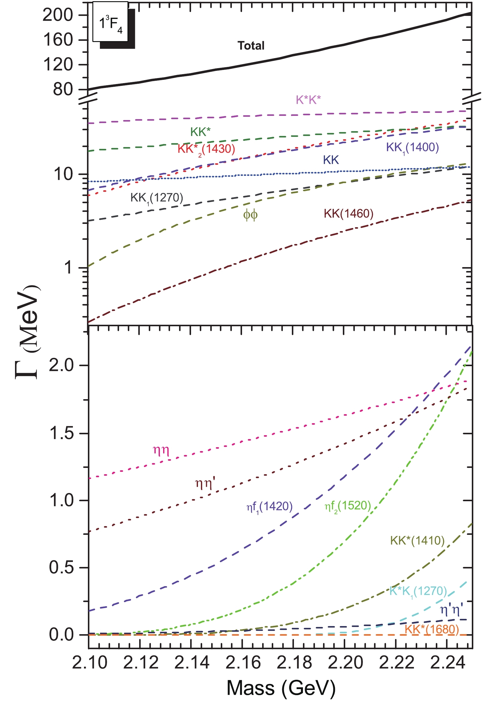
Figure 3. (color online) Variation of the decay widths for the
$ 1^3F_4 $ $ s\bar{s} $ state with its mass.There might be some experimental evidence for this state. The LASS Collaboration observed a rather narrow
$ 4^{++} $ resonance (denoted by$ f_4(2210) $ ) with a mass and width of$ M = 2209^{+17}_{-15} $ MeV and$ \Gamma = 60^{+107}_{-57} $ MeV, by an analysis of the$ K^+K^- $ mass spectrum from the reaction$ K^-p\to K^+K^- \Lambda $ [40]. The mass and width values of$ f_4(2210) $ are consistent with those obtained by MARK III for the$ X(2200) $ from the reaction$ J/\psi\to \gamma KK $ [84]. A similar resonance with a mass and width of$ M = 2231\pm 10 $ MeV and$ \Gamma = (130\pm 50) $ MeV was also observed in the$ \phi\phi $ final state by WA67 (CERN SPS) [85]. The$ f_4(2210) $ might be an assignment of the$ 1^3F_4 $ $ s\bar{s} $ state [16, 80].Considering the
$ f_4(2210) $ resonance as the$ 1^3F_4 $ $ s\bar{s} $ state, we find that our predicted decay width$ \Gamma_{\rm total}\simeq 161 \; \mathrm{MeV} $

(45) is consistent with the observed width from experiments. The branching fractions for the dominant decay modes
$ KK $ ,$ KK^* $ ,$ K^*K^* $ ,$ KK_2^*(1430) $ ,$ KK_1(1270) $ , and$ KK_1(1400) $ are predicted to be ~7%, ~18%, ~28%, ~16%, ~6%, and ~15%, respectively. Furthermore, it is found that the$ \phi\phi $ mode also plays an important role in the decay. Its branching fraction may reach up to ~6%, which is comparable with that of the$ KK $ mode. The partial width ratio between$ \phi\phi $ and$ KK $ is predicted to be:$ R_{\phi\phi/KK} = \frac{\Gamma(\phi\phi)}{\Gamma(KK)}\simeq 0.82, $

(46) which can be used to test the nature of the
$ f_4(2210) $ . The fairly large decay rates of$ f_4(2210) $ into the$ KK $ and$ \phi\phi $ final states may explain why it has been seen in these channels. To definitely establish the$ 1^3F_4 $ $ s\bar{s} $ state and confirm the nature of$ f_4(2210) $ more accurate observations in the dominant decay modes are needed in future experiments. -
There is no hint about the
$ 1^3F_3 $ $ s\bar{s} $ state from experiments. Our quark model predicted mass is$ M = 2128 $ MeV, which is in good agreement with the prediction with the covariant oscillator quark model [19], while it is about 100 MeV smaller than the predictions with the relativized quark model [17, 18] and the relativistic quark model [20]. The mass of$ 1^3F_3 $ might overlap significantly with that of$ 1^3F_2 $ with a mass splitting$ \sim 10-30 $ MeV [17-19]. If$ f_2(2150) $ does indeed correspond to the$ 1^3F_2 $ $ s\bar{s} $ state, the mass of the$ 1^3F_3 $ $ s\bar{s} $ state is most likely to be in the range ~2120-2160 MeV. According to our analysis of the strong decay properties (see Table 7), this state might be a broad state with a width of:$ \Gamma_{\rm total}\simeq 245 \; \mathrm{MeV}. $

(47) The dominant decay channels might be
$ KK_2^*(1430) $ ,$ KK^* $ ,$ K^*K^* $ , and$ KK_1(1270) $ , and their branching fractions are predicted to be ~56%, ~13%, ~8%, and ~15%, respectively. It is interesting to find that the decay rate into the$ \eta f_2'(1525) $ channel is sizeable, and the branching fraction could reach up to ~6.5%. The$ \eta f_2'(1525) $ may be a useful channel for searching for the missing$ 1^3F_3 $ $ s\bar{s} $ state in experiments. Our main predictions of the strong decay properties are consistent with those predicted in Ref. [16]. -
The
$ 1^1F_3 $ $ s\bar{s} $ state is not established. Our quark model predicted mass is$ M = 2111 $ MeV, which is in good agreement with the prediction with the covariant oscillator quark model [19], while it is about 100 MeV smaller than the predictions with the relativized quark model [17, 18] and the relativistic quark model [20]. According to our analysis of the strong decay properties (see Table 7), this state might be a moderately broad state with a width of:$ \Gamma_{\rm total}\simeq 178\; \mathrm{MeV}. $

(48) The decays are governed by the
$ KK_2^*(1430) $ channel with a branching fraction ~60%. The$ KK^* $ and$ K^*K^* $ decay modes are another two important decay modes, with comparable branching fractions of ~12%-18%. Our main predictions are consistent with those predicted in Ref. [16]. As an attractive decay mode for observations, the$ \eta \phi $ channel may have a sizeable branching fraction of ~4%, which is about three times smaller than the value predicted in Ref. [16]. -
The
$ 2^3D_1 $ $ s\bar{s} $ state is not established. In various quark models, its mass is predicted to be in the range ~2.26-2.35 GeV [17-20]. Our predicted mass$ M = 2272 $ MeV is comparable with the other model predictions within an uncertainty of about$ \pm60 $ MeV. According to our analysis of the strong decay properties (see Table 8), this state might be a broad state with a width of:$ \Gamma_{\rm total}\simeq 322\; \mathrm{MeV}, $

(49) which mainly decays into the
$ KK(1460) $ ,$ K^*K^* $ ,$ KK_2^*(1430) $ ,$ KK_1(1270) $ ,$ K^*K_1(1270) $ , and$ KK^*(1410) $ final states with branching fractions ~12%, ~9%, ~8%, ~27%, ~21%, and ~10%, respectively. Furthermore, the$ KK $ and$ KK^* $ modes have some sizeable contributions to the decays. They have comparable branching fractions of ~2%. The decay properties for the$ 2^3D_1 $ $ s\bar{s} $ state roughly agree with the predictions in Refs. [6, 13]. -
There is no hint about the
$ 2^3D_2 $ $ s\bar{s} $ state from experiments. In our nonrelativistic quark model calculation, its mass is predicted to be$ M = 2297 $ MeV, which is slightly smaller than the previous quark model predictions of ~2320-2350 MeV [17-20]. According to our analysis of the strong decay properties (see Table 9), this state might be a moderately broad state with a width of:$ \Gamma_{\rm total}\simeq 232\; \mathrm{MeV}, $

(50) which mainly decays into the
$ KK^*(1410) $ ,$ KK_2^*(1430) $ ,$ K^*K_1(1270) $ , and$ KK_3^*(1780) $ final states. Their branching fractions are predicted to be ~30%, ~21%, ~10%, and ~13%, respectively. Furthermore, the$ KK^* $ ,$ K^*K^* $ , and$ KK_1(1400) $ modes have some sizeable contributions to the decays, with comparable branching fractions of ~3%-7%. -
There is no hint about the
$ 2^3D_3 $ $ s\bar{s} $ state from experiments. In our nonrelativistic quark model calculation, its mass is predicted to be$ M = 2285 $ MeV, which is slightly ($ 50-80 $ MeV) smaller than the previous quark model predictions ~2340-2360 MeV [17-20]. According to our analysis of the strong decay properties (see Table 8), this state might be the narrowest of the$ 2D $ states, with a width of:$ \Gamma_{\rm total}\simeq 136\; \mathrm{MeV}. $

(51) The
$ 2^3D_3 $ $ s\bar{s} $ state mainly decays into the$ KK(1460) $ ,$ KK^*(1410) $ ,$ K^*K^* $ ,$ KK^*_2(1430) $ , and$ KK_1(1270) $ final states, with branching fractions ~19%, ~13%, ~12%, ~11%, and ~17%, respectively. Furthermore, the$ KK $ ,$ KK^* $ ,$ KK_1(1400) $ , and$ K^*K_1(1270) $ modes may have some sizeable contributions to the decays, with comparable branching fractions of ~3%-8%. -
There is no hint about the
$ 2^1D_2 $ $ s\bar{s} $ state from experiments. In our nonrelativistic quark model calculation, its mass is predicted to be$ M = 2282 $ MeV, which is slightly ($ 40-60 $ MeV) smaller than the previous quark model predictions of ~2320-2340 MeV [18-20]. According to our analysis of the strong decay properties (see Table 9), this state might have a moderate width of:$ \Gamma_{\rm total}\simeq 208 \; \mathrm{MeV}, $

(52) and mainly decay into the
$ KK^*(1410) $ ,$ KK^*_2(1430) $ , and$ K^*K_1(1270) $ final states, with comparable branching fractions of ~14%-27%. Furthermore, the$ 2^1D_2 $ $ s\bar{s} $ state may have sizeable decay rates into the$ KK^* $ ,$ K^*K^* $ , and$ KK^*_0(1430) $ final states, with comparable branching fractions of ~5%. -
The vector meson resonance
$ \phi(2170) $ (often denoted$ Y (2175) $ in the literature) was first observed with a mass$ M = (2175\pm 35) $ MeV and a width$ \Gamma = 58\pm 36 $ MeV by the$ BaBar $ Collaboration in the initial state radiation (ISR) process$ e^+e^-\to \gamma_{ISR}\phi f_0(980) $ [86]. In addition$ BaBar $ also observed evidence of$ \phi(2170) $ in the process$ e^+e^-\to \gamma_{ISR}\phi \eta $ [55]. Subsequently, the$ \phi(2170) $ was confirmed in the BES experiment in$ J/\psi\to \eta \phi f_0(980) $ ,$ J/\psi\to \eta \phi \pi^+\pi^- $ , and$ e^+e^-\to \eta Y(2175) $ [87-89], and in the Belle experiment in$ e^+e^-\to \phi \pi^+\pi^- $ [90]. Recently, a partial wave analysis (PWA) of the process$ e^+e^-\to K^+K^-\pi^0\pi^0 $ was performed by the BESIII Collaboration. It was observed that the$ \phi(2170) $ has a sizable partial width to$ K^+(1460)K^- $ ,$ K^+_1(1400)K^- $ , and$ K^+_1(1270)K^- $ , but a much smaller partial width to$ K^{*+}(892)K^{*-}(892) $ and$ K^{*+}(1410)K^{-} $ [11]. Very recently, the$ \phi(2170) $ was also clearly seen in the Born cross sections of$ e^+e^-\to \phi\eta' $ by the BESIII Collaboration [12]. It should be mentioned that some measurements of the processes$ e^+e^-\to K^+K^-K^+K^- $ [91-93],$ \phi K^+K^- $ [93], and$ K^+K^- $ [94, 95] have been carried out at$ BaBar $ and BESIII, but no significant signals of$ \phi(2170) $ were found in the these reactions.There are long-standing puzzles about the nature of
$ \phi(2170) $ . Many interpretations, such as a conventional$ 3^3S_1 $ or$ 2^3D_1 $ $ s\bar{s} $ state [6, 13-16], an$ \bar{s}sg $ hybrid state [96, 97], a tetraquark state [98-105], a$ \Lambda\bar{\Lambda} $ bound state [106-108], or a resonant state of the$ \phi KK $ system [109, 110], have been widely discussed in the literature. However, no interpretation has yet been established. In the following, we discuss the possibilities of$ \phi(2170) $ as the conventional$ 3^3S_1 $ and$ 2^3D_1 $ $ s\bar{s} $ states, or a mixing state between them. -
The mass of the
$ \phi(3S) $ ($ 3^3S_1 $ $ s\bar{s} $ ) state is estimated to be in the range ~2.05-2.25 GeV in various quark models [6, 17-20]. Concerning the mass, the$ \phi(2170) $ is a good candidate for the$ \phi(3S) $ state. Our predicted mass$ M = 2198 $ MeV is close to the upper limit of the observations. It should be mentioned that the measured mass of$ \phi(2170) $ has a fairly large uncertainty, with a range of ~2.05-2.20 GeV. In this possible range we plot the strong decay properties as functions of the initial state mass in Fig. 4. It is found that the partial widths for the$ KK^*(1410) $ ,$ K^*K^* $ ,$ KK_1(1400) $ , and$ KK_1(1270) $ decay modes are very sensitive to the mass of the$ \phi(2170) $ . Taking three typical masses of$ 2079 $ ,$ 2135 $ , and$ 2175 $ MeV for$ \phi(2170) $ , we also give our results in Table 10.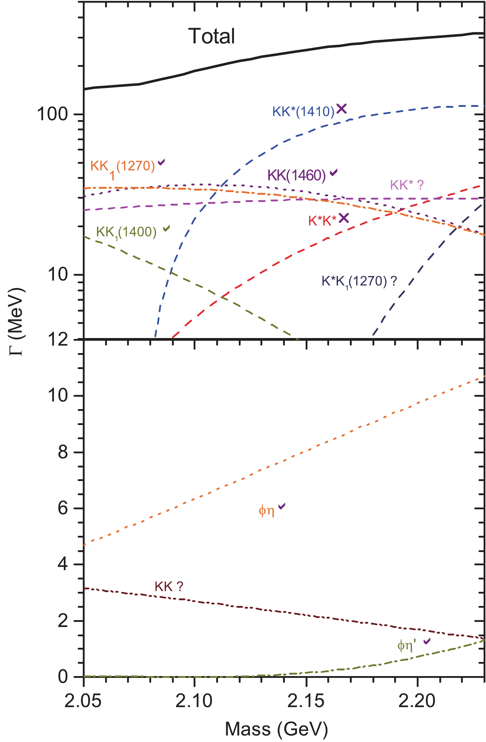
Figure 4. (color online) Variation of the decay widths for the
$ 3^3S_1 $ $ s\bar{s} $ state with its mass. The observed decay modes of$ \phi(2170) $ are labeled with$ "\checkmark" $ , decay modes which have not been seen experimentally are labeled with$ "\times" $ , and decay modes which await further confirmation are labeled with$ "?".$ If the
$ \phi(2170) $ mass is around$ 2135-2175 $ MeV, as an assignment of the$ \phi(3S) $ state, the$ \phi(2170) $ should be a moderately broad state with a width of$ \sim 240-270 $ MeV. Although the predicted width is close to the upper limit of the observed value from Belle [90], the decay modes are inconsistent with the observations. For example, the$ KK^*(1410) $ and$ K^*K^* $ decay modes, as the main modes of the$ \phi(3S) $ , were not observed in the recent BESIII experiment [11].On the other hand, if a smaller mass of ~2.08-2.1 GeV is taken for the
$ \phi(2170) $ , one can find that the$ \phi(2170) $ has a relatively narrow width of ~170-200 MeV, and dominantly decays into the$ KK^* $ ,$ KK(1460) $ ,$ KK_2^*(1430) $ ,$ KK_1(1270) $ , and$ KK_1(1400) $ final states. In this case, as an assignment of$ \phi(3S) $ , both the predicted width and decay modes of$ \phi(2170) $ are consistent with the present observations. The branching fractions for the interesting decay modes$ \phi\eta $ and$ \phi\eta' $ in experiments are predicted to be$ O(10^{-2}) $ and$ O(10^{-3}) $ , respectively.As a whole, the possibility of the
$ \phi(2170) $ as a candidate for the$ \phi(3S) $ cannot be excluded. The decay properties of the$ \phi(3S) $ strongly depend on its mass. Precise measurements of branching fraction ratios between the main decay modes and the resonance parameters are crucial to confirm whether the$ \phi(2170) $ can be assigned to the$ \phi(3S) $ state or not. -
Concerning the mass, there is the possibility to assign
$ \phi(2170) $ as the$ \phi(2D) $ ($ 2^3D_1 $ $ s\bar{s} $ ) state. The mass of the$ \phi(2D) $ predicted from various quark models is$ \sim 2.25-2.35 $ GeV [6,17-20], which is about$ 100-150 $ MeV higher than that of the$ \phi(2170) $ . Considering$ \phi(2170) $ as the$ 2^3D_1 $ $ s\bar{s} $ t state, we study the strong decay properties. By varying the mass of the$ \phi(2170) $ in its possible range of$ \sim 2.05-2.20 $ GeV, we plot the strong decay widths in Fig. 5. Taking three typical values,$ 2079 $ ,$ 2135 $ , and$ 2175 $ MeV, for the$ \phi(2170) $ , we also give our predictions of the decay properties in Table 10. It is found that the partial widths of$ KK^*(1410) $ ,$ KK_1(1270) $ ,$ KK_1(1400) $ , and$ K^*K^*(1270) $ are sensitive to the mass of the$ \phi(2170) $ .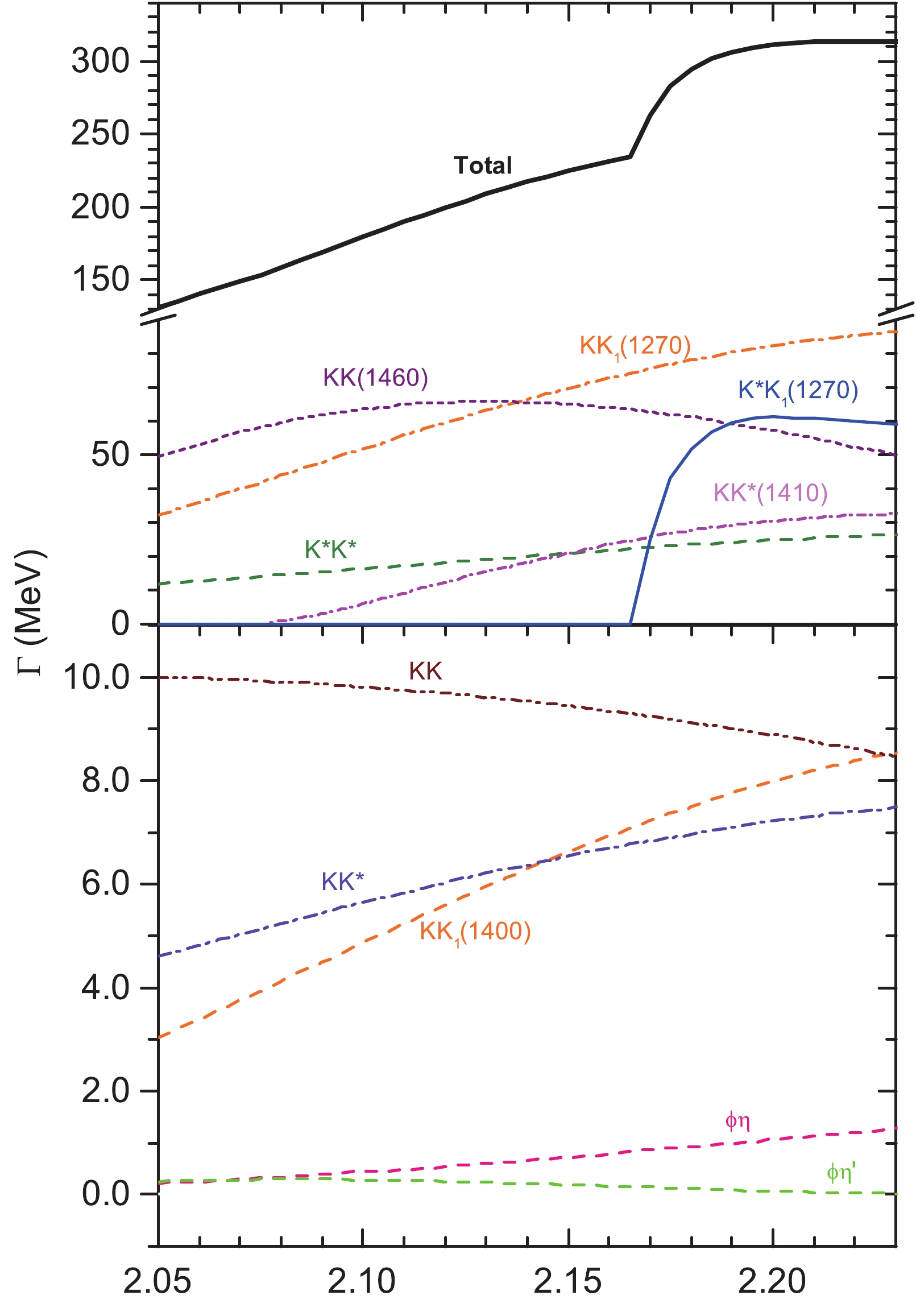
Figure 5. (color online) Variation of the decay widths for the
$ 2^3D_1 $ $ s\bar{s} $ state with its mass.If the mass of
$ \phi(2170) $ is around$ 2175 $ MeV, as an assignment of the$ \phi(2D) $ state,$ \phi(2170) $ should be a broad state with a width of$ \sim 300 $ MeV, which is too broad to be comparable with the observation. Moreover, the decay modes are inconsistent with the observations. For example, the$ KK^*(1410) $ and$ K^*K^* $ decay modes, as the main modes of$ \phi(2D) $ , were not observed by the recent BESIII experiment [11].On the other hand, if the mass of
$ \phi(2170) $ is in the range ~2079-2135 MeV, as an assignment of$ \phi(2D) $ , the width of the$ \phi(2170) $ is predicted to be$ \sim 175-225 $ MeV, which is close to the upper limit of the observations. The$ KK_1(1400) $ ,$ KK(1460) $ ,$ KK_1(1270) $ decay modes, as the main decay modes, were observed by the recent BESIII experiments as well [11]. However, it is difficult to understand why the other main decay mode,$ K^*K^* $ , was not observed by the recent BESIII experiments [11]. A slight mixing with the$ \phi(3S) $ state (for example with a mixing angle$ \theta\simeq-20^{\circ} $ ) can strongly suppress partial widths of the$ KK^* $ ,$ KK^*(1410) $ , and$ KK^*_2(1430) $ mode, but the partial width of$ K^*K^* $ is still large, and insensitive to the mixing angle (see Fig. 6). Confirmation of the$ K^*K^* $ decay mode and accurate measurements of the resonance parameters for the$ \phi(2170) $ are crucial for understanding its nature.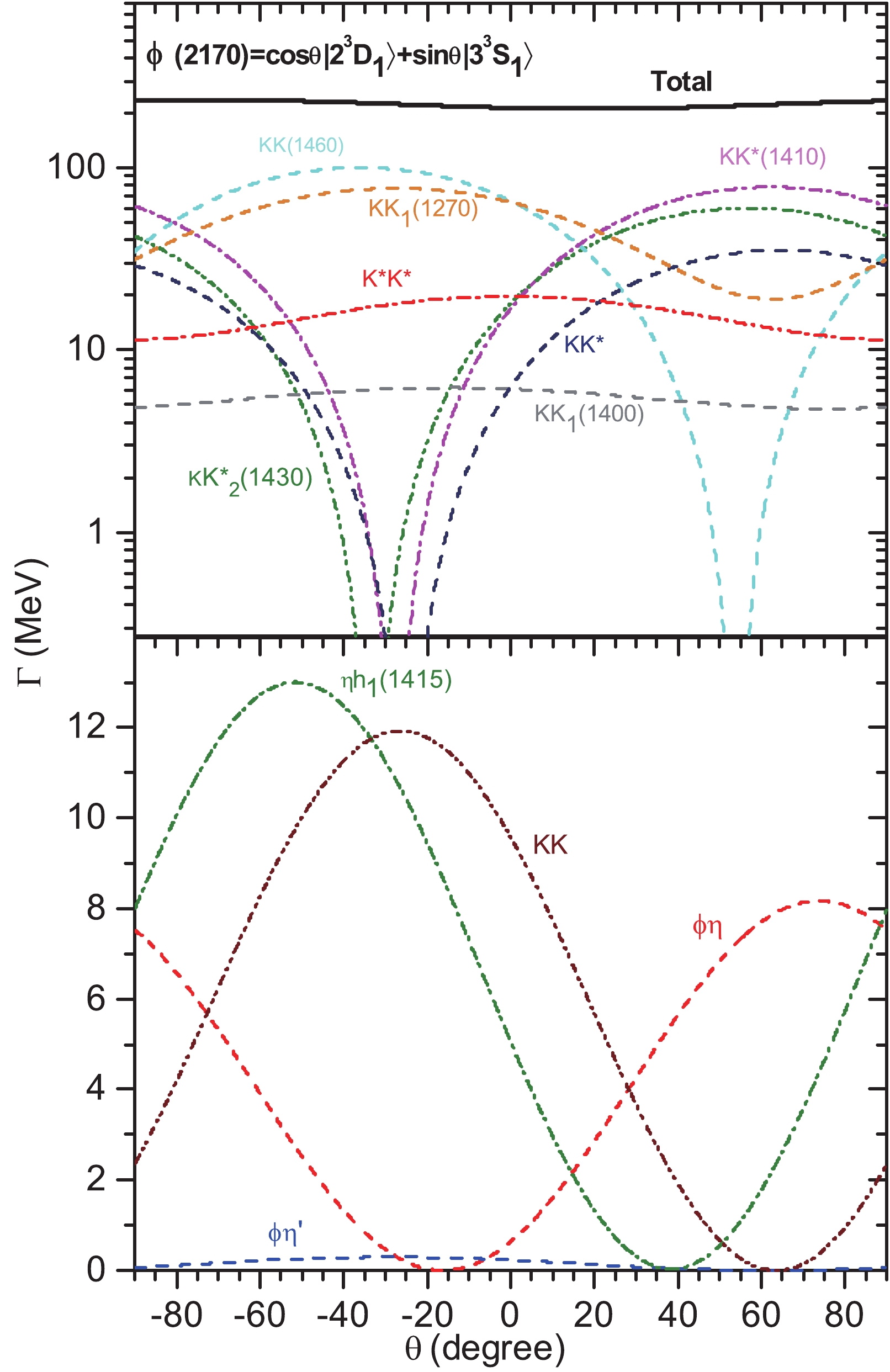
Figure 6. (color online) Strong decay of
$ \phi(2170) $ versus mixing angle$ \theta $ Finally, it should be mentioned that according to the quark model predictions the mass difference between
$ \phi(2D) $ and$ \phi(3S) $ states is$ \sim 100 $ MeV, and both of them have a fairly broad width of$ \sim 200-300 $ MeV. Thus, both$ \phi(2D) $ and$ \phi(3S) $ may overlap with each other significantly around the energy range$ \sim 2.2\pm 0.1 $ GeV. Furthermore, both$ \phi(2D) $ and$ \phi(3S) $ have similar strong decay properties. For example, both of them dominantly decay into$ KK_1(1400) $ ,$ KK(1460) $ ,$ KK_1(1270) $ ,$ KK_1(1400) $ , and$ KK^*_2(1430) $ . The above facts indicate that it may be hard to distinguish these two overlapping resonances from the invariant mass distributions of the final states. Thus, the$ \phi(2170) $ resonance observed in some reactions may be a structure caused by two largely overlapping resonances$ \phi(2D) $ and$ \phi(3S) $ . This may explain the fairly large uncertainties for the resonance parameters extracted from different experiments. -
The
$ 3^3P_0 $ $ s\bar{s} $ state is not established. Our quark model predicted mass is$ M = 2434 $ MeV, which is in good agreement with the predictions with the relativized quark model [17, 18]. However, it is about$ 80-150 $ MeV larger than those predicted in Refs. [19, 20]. According to our analysis of the strong decay properties (see Table 11), this state might be a broad state with a width of:Table 11-continued from previous page Mode State $ \Gamma_{\rm th} $ /MeV

$ Br$ (%)

Amps. /(GeV $ ^{-1/2} $ )

State $ \Gamma_{\rm th} $ /MeV

$ Br$ (%)

Amps. /(GeV $ ^{-1/2} $ )

$ KK_1(1400) $ 

0.8 0.2 $ ^3P_0 $ = 0.012

11 7.8 $ ^3P_2 $ = −0.045

$ ^3F_2 $ = −0.001

$ K^*(892)K_1(1270) $ 

12 3.5 $ ^3P_0 $ = −0.055

21 15 $ ^3P_2 $ = 0.004

$ ^3F_2 $ = −0.038

$ ^5P_2 $ = 0.024

$ ^5F_2 $ = −0.054

$ K^*(892)K_1(1400) $ 

15 4.5 $ ^3P_0 $ = 0.072

2.5 1.7 $ ^3P_2 $ = −0.026

$ ^3F_2 $ = 0.004

$ ^5P_2 $ = −0.006

$ ^5F_2 $ = 0.006

$ KK^*(1680) $ 

$ \cdots $ 

$ \cdots $ 

$ \cdots $ 

1.4 1.0 $ ^3D_2 $ = −0.018

$ KK_2(1770) $ 

92 27 $ ^5D_0 $ = 0.160

5.8 4.0 $ ^5S_2 $ = 0.001

$ ^5D_2 $ = −0.023

$ ^5G_2 $ = −0.031

$ KK_2'(1820) $ 

4.6 1.3 $ ^5D_0 $ = −0.039

4.3 3.0 $ ^5S_2 $ = 0.014

$ ^5D_2 $ = 0.032

$ ^5G_2 $ = 0.002

$ KK^*_3(1780) $ 

$ \cdots $ 

$ \cdots $ 

$ \cdots $ 

16 11 $ ^7D_2 $ = 0.060

$ ^7G_2 $ = 0.024

$ \eta f_1(1420) $ 

12 3.5 $ ^3P_0 $ = −0.213

1.8 1.2 $ ^3P_2 $ = −0.073

$ ^3F_2 $ = −0.033

$ \eta f_2'(1525) $ 

$ \cdots $ 

$ \cdots $ 

$ \cdots $ 

3.3 2.2 $ ^5P_2 $ = 0.084

$ ^5F_2 $ = −0.079

$ \eta' f_1(1420) $ 

0.04 0.01 $ ^3P_0 $ = −0.016

0.4 0.3 $ ^3P_2 $ = 0.041

$ ^3F_2 $ = −0.017

$ \phi h_1(1415) $ 

$ \cdots $ 

$ \cdots $ 

$ \cdots $ 

1.4 1.0 $ ^3P_2 $ = −0.068

$ ^3F_2 $ = 0.007

$ ^5P_2 $ = 0.052

$ ^5F_2 $ = 0.009

Total 346 100 145 100 $ \Gamma_{\rm total}\simeq 346 \; \mathrm{MeV}, $

(53) which dominantly decays into the
$ K^*K^* $ ,$ K^*K_2^*(1430) $ ,$ KK_1(1270) $ , and$ KK_2(1770) $ final states, with branching fractions ~12%, ~9%, ~25%, and ~27%, respectively. Few studies of the strong decays of the higher$ 3P $ -wave$ s\bar{s} $ states are found in the literature.Recently, by an amplitude analysis of the
$ K_SK_S $ system produced in radiative$ J/\psi $ decays, an isoscalar scalar$ 0^{++} $ state,$ f_0(2410) $ , was found at BESIII with a$ 35\sigma $ significance [7]. The mass and width were determined to be$ M = (2411\pm17) $ MeV and$ \Gamma = (348\pm18 $ $ ^{+23}_{-1}) $ MeV, respectively, which are obviously different from those for the$ f_0(2330) $ resonance listed by the PDG [1]. It is interesting to find that both the mass and width of the newly observed state$ f_0(2410) $ are in good agreement with our predictions by considering it as the$ 3^3P_0 $ $ s\bar{s} $ state. Furthermore, with this assignment we obtain sizeable branching fractions for the$ KK $ and$ \phi\phi $ channels:$ Br[f_0(2410)\to KK/\phi\phi]\simeq {\cal{O}}(1 \%-2 \%), $

(54) which may explain why the
$ f_0(2410) $ can be established in the$ K_SK_S $ final state. It should be mentioned that flavor mixing between$ s\bar{s} $ and$ n\bar{n} $ may exist in the$ ^3P_0 $ state [26], which may affect our predictions. To better understand the nature of the$ f_0(2410) $ and confirm our assignment, more observations of some interesting decay channels, such as$ \phi\phi $ ,$ KK_1(1400) $ and$ K^*K^* $ , are needed in future experiments. -
The
$ 3^3P_2 $ $ s\bar{s} $ state is not established. Our quark model predicted mass is$ M = 2466 $ MeV, which is in good agreement with the predictions with the relativized quark model [17, 18]. The mass splitting between the$ 3^3P_2 $ and$ 3^3P_0 $ states is predicted to be about$ 32 $ MeV, which is comparable with those predicted in Refs. [18, 20]. If the$ f_0(2410) $ does indeed correspond to the$ 3^3P_0 $ $ s\bar{s} $ state, the mass of the$ 3^3P_2 $ state might be around$ 2440-2450 $ MeV.According to our analysis of the strong decay properties (see Table 11), this state might have a moderate width of:
$ \Gamma_{\rm total}\simeq 145 \; \mathrm{MeV}, $

(55) and dominantly decay into the
$ K^*K(1460) $ ,$ K^*K^* $ ,$ K^*K_2^*(1430) $ ,$ KK_3^*(1780) $ , and$ K^*K_1(1270) $ final states, with branching fractions ~12%, ~10%, ~13%, ~11%, and ~15%, respectively. The decay rates into the$ KK $ and$ \phi\phi $ final states might be sizeable, and the branching fractions are predicted to be about 2% and 1%, respectively.Some signals of the
$ 3^3P_2 $ $ s\bar{s} $ state might have been observed in some processes, such as$ J/\psi\to \gamma \phi\phi/\gamma\eta\eta $ at BESIII [8, 111]. However, the resonance parameters may be hard to extract from the data due to strong effects from some nearby resonances and backgrounds. -
The
$ 3^3P_1 $ $ s\bar{s} $ state is not established. Our quark model predicted mass is$ M = 2470 $ MeV, which is in good agreement with the other predictions in Refs. [18, 19]. The mass splitting between the$ 3^3P_1 $ and$ 3^3P_0 $ states is predicted to be about$ 30-40 $ MeV in most quark models (See Table 2). If the$ f_0(2410) $ does indeed correspond to the$ 3^3P_0 $ state, the mass of$ 3^3P_1 $ might be around$ 2440-2450 $ MeV, and it may overlap significantly with the$ 3^3P_2 $ state. According to our analysis of the strong decay properties (see Table 12), this state might be a broad state with a width of:$ \Gamma_{\rm total}\simeq 298 \; \mathrm{MeV}. $

(56) The
$ 3^3P_1 $ $ s\bar{s} $ state has relatively large decay rates into the$ KK^*(1410) $ ,$ KK_2^*(1430) $ ,$ K^*K_2^*(1430) $ ,$ KK_2(1770) $ ,$ KK_3^*(1780) $ channels, with comparable branching fractions of ~10% (details are listed in Table 12). The$ K^*K_1(1270) $ mode may play a crucial role in the decays, and the branching fraction for this channel may reach up to ~15%. Moreover, the decay rates into the$ KK^* $ and$ \phi\phi $ final states might be sizeable, with branching fractions predicted to be ~4.1% and ~1.1%, respectively. The$ \phi\phi $ ,$ KK^* $ ,$ K^*K^* $ and$ KK_2^*(1430) $ channels might be good channels for looking for the missing$ 3^3P_1 $ $ s\bar{s} $ state.Table 12-continued from previous page Mode State $ \Gamma_{\rm th} $ /MeV

$ Br $ (%)

Amps. /(GeV $ ^{-1/2} $ )

State $ \Gamma_{\rm th} $ /MeV

$ Br $ (%)

Amps. /(GeV $ ^{-1/2} $ )

$ \phi\phi $ 

3.3 1.1 $ ^5D_1 $ = 0.067

$ \cdots $ 

$ \cdots $ 

$ \cdots $ 

$ KK_1(1270) $ 

12 4.2 $ ^3P_1 $ = 0.045

0.8 0.3 $ ^3P_1 $ = −0.012

$ KK_1(1400) $ 

2.0 0.7 $ ^3P_1 $ = 0.019

0.9 0.3 $ ^3P_1 $ = −0.013

$ K^*(892)K_1(1270) $ 

45 15 $ ^1P_1 $ = −0.009

41 15 $ ^1P_1 $ = −0.003

$ ^3P_1 $ = 0.023

$ ^3P_1 $ = 0.003

$ ^5P_1 $ = 0.082

$ ^5P_1 $ = −0.052

$ ^5F_1 $ = 0.055

$ ^5F_1 $ = 0.085

$ K^*(892)K_1(1400) $ 

4.9 1.7 $ ^1P_1 $ = 0.004

18 6.7 $ ^1P_1 $ = −0.078

$ ^3P_1 $ = 0.037

$ ^3P_1 $ = −0.004

$ ^5P_1 $ = 0.006

$ ^5P_1 $ = −0.004

$ ^5F_1 $ = −0.006

$ ^5F_1 $ = −0.008

$ KK^*(1680) $ 

0.7 0.2 $ ^3S_1 $ = 0.010

5.2 1.9 $ ^3S_1 $ = 0.004

$ ^3D_1 $ = 0.008

$ ^3D_1 $ = 0.035

$ KK_2(1770) $ 

32 11 $ ^5D_1 $ = −0.091

0.3 0.1 $ ^5D_1 $ = 0.009

$ KK_2(1820) $ 

2.0 0.7 $ ^5D_1 $ = −0.024

0.2 0.1 $ ^5D_1 $ = 0.008

$ KK^*_3(1780) $ 

40 13 $ ^7D_1 $ = 0.098

50 19 $ ^7D_1 $ = 0.115

$ ^7G_1 $ = −0.026

$ ^7G_1 $ = 0.027

$ \eta f_0(1370) $ 

0.23 0.08 $ ^1P_1 $ = 0.028

$ \cdots $ 

$ \cdots $ 

$ \cdots $ 

$ \eta f_1(1420) $ 

4.4 1.5 $ ^3P_1 $ = 0.126

$ \cdots $ 

$ \cdots $ 

$ \cdots $ 

$ \eta f_2'(1525) $ 

6.2 2.1 $ ^5P_1 $ = 0.135

$ \cdots $ 

$ \cdots $ 

$ \cdots $ 

$ ^5F_1 $ = 0.083

$ \eta' f_0(1370) $ 

0.05 0.02 $ ^1P_1 $ = 0.015

$ \cdots $ 

$ \cdots $ 

$ \cdots $ 

$ \eta' f_1(1420) $ 

1.4 0.5 $ ^3P_1 $ = −0.086

$ \cdots $ 

$ \cdots $ 

$ \cdots $ 

$ \phi f_0(1370) $ 

$ \cdots $ 

$ \cdots $ 

$ \cdots $ 

$<0.01 $ 

$<0.01 $ 

$ \cdots $ 

$ \phi h_1(1415) $ 

6.5 2.2 $ ^1P_1 $ = −0.005

$ \cdots $ 

$ \cdots $ 

$ \cdots $ 

$ ^3P_1 $ = 0.137

$ ^5P_1 $ = 0.115

$ ^5F_1 $ = −0.011

Total 298 100 269 100 -
The
$ 3^1P_1 $ $ s\bar{s} $ state is not established. Our quark model predicted mass is$ M = 2435 $ MeV, which is comparable with the predictions in Refs. [18-20]. The mass splitting between the$ 3^1P_1 $ and$ 3^3P_0 $ states is predicted to be about a few MeV. If the$ f_0(2410) $ does indeed correspond to the$ 3^3P_0 $ , the mass of the$ 3^1P_1 $ state might be around$ 2410 $ MeV as well. According to our analysis of the strong decay properties (see Table 12), this state might be a broad state with a width of$ \Gamma_{\rm total}\simeq 269 \; \mathrm{MeV}. $

(57) The
$ 3^1P_1 $ $ s\bar{s} $ state has relatively large decay rates into the$ K^*K^* $ ,$ K^*K(1460) $ ,$ KK_2^*(1430) $ ,$ K^*K_2(1430) $ ,$ K^*K_1(1270) $ ,$ K^*K_1(1400) $ ,$ KK^*(1410) $ , and$ KK_3^*(1780) $ channels, with comparable branching fractions of ~7%-20% (details are listed in Table 12). The decay rates into the$ \phi\eta $ and$ \phi\eta' $ final states are sizeable, and the branching fractions are predicted to be ~1.7% and ~0.6%, respectively. The$ \phi\eta $ and$ \phi\eta' $ might be good channels for searching for the missing$ 3^1P_1 $ $ s\bar{s} $ state. -
The flavor mixing between
$ n\bar{n} $ and$ s\bar{s} $ plays an important role for the low-lying isoscalar$ 0^{-+} $ states. However, the spectroscopic mixing for the higher$ s\bar{s} $ excitation,$ 4^1S_0 $ , may be small [17]. The mass for the higher$ 4^1S_0 $ $ s\bar{s} $ ($ J^{PC} = 0^{-+} $ ) state is estimated to be$ \sim 2580 $ MeV within our nonrelativistic potential model, which is consistent with the prediction with the relativized quark model [17, 18], although our predicted mass is notably (~150-320 MeV) larger than that predicted in Refs. [19, 20].Using the mass and wave function obtained from our potential model calculations, we further estimate the strong decay properties. Our results are listed in Table 13. It is found that the
$ 4^1S_0 $ $ s\bar{s} $ has a rather broad width of$ \Gamma_{\rm total}\simeq 409 \; \mathrm{MeV}, $

(58) and dominantly decays into the
$ K^*K_1(1400) $ final state with a branching fraction ~15%. Furthermore, the$ 4^1S_0 $ $ s\bar{s} $ state has large decay rates into the$ KK^* $ ,$ KK^*(1410) $ ,$ K^*K_1(1270) $ ,$ K^*K^*(1410) $ ,$ KK^*_3(1780) $ ,$ K^*K^* $ , and$ KK^*_2(1430) $ final states, with comparable branching fractions of ~8%-11%.In 2016, the BESIII Collaboration observed a new resonance
$ X(2500) $ , with a mass of$ 2470^{+15}_{-19} $ $ ^{+101}_{-23} $ MeV and a width of$ 230^{+64}_{-35} $ $ ^{+56}_{-33} $ MeV in$ J/\psi\to \gamma \phi\phi $ [8]. The preferred spin-parity numbers for the$ X(2500) $ are$ J^{PC} = 0^{-+} $ [8]. The newly observed state$ X(2500) $ may be identified as the$ 4^1S_0 $ $ s\bar{s} $ state. With this assignment, its measured mass, width, and spin-parity numbers can be naturally understood in our calculations. The decay rate into the$ \phi\phi $ final state is also sizeable, and the branching fraction is predicted to be:$ Br[X(2500)\to \phi\phi]\simeq 0.71 \%,$

(59) which can explain why
$ X(2500) $ was seen in the$ \phi\phi $ final state as well.Some other interpretations of
$ X(2500) $ , such as the fourth radial excitation of$ \eta' $ meson (i.e.$ \eta'(5S) $ ) [112], the$ 5^1S_0 $ $ s\bar{s} $ state [9, 113], or the$ ss\bar{s}\bar{s} $ tetraquark state with$ J^{PC} = 0^{-+} $ [114, 115], can be found in the literature. In some works [116], the$ 4^1S_0 $ $ s\bar{s} $ state was suggested to be an assignment for the resonance$ \eta(2225) $ listed by the PDG [1]. To clarify the nature of$ X(2500) $ and establish the$ 4^1S_0 $ $ s\bar{s} $ state, more observations of the dominant decay modes, such as$ KK^* $ and$ KK^*_2(1430) $ , are needed in future experiments. -
As a higher excitation, the mass of the
$ 4^3S_1 $ $ s\bar{s} $ state predicted in theory spans a large range, ~2.47-2.63 GeV, with fewer constraints from experiments. With a linear potential, both our nonrelativistic potential model and the relativized quark model [17, 18] give a similar mass,$ M\simeq 2625 $ MeV. In Ref. [19], by using a covariant oscillator quark model with one-gluon-exchange effects, the authors predicted a moderate mass$ M\simeq 2540 $ MeV. In Ref. [20], with a QCD-motivated relativistic quark model, the authors obtained a small mass$ M\simeq 2472 $ MeV, which is comparable with the prediction with the modified relativized quark model by replacing the linear potential with a screening potential [6]. Observations of the$ 4^3S_1 $ $ s\bar{s} $ state are crucial for testing the various models and developing QCD-motivated potential models.To provide useful information for looking for the
$ 4^3S_1 $ $ s\bar{s} $ state in experiments, we further estimate the strong decay properties with the mass and wave function obtained from our potential model calculations. Our results are listed in Table 13. This state might have a moderate width$ \Gamma\sim 227 $ MeV, and mainly decays into$ K^*(892)K^*(892) $ ,$ KK^*(892) $ ,$ KK^*(1410) $ ,$ K^*(892)K(1460) $ ,$ K^*(892)K_1(1270) $ , and$ K_1(1270)K_1(1270) $ . The$ 4^3S_1 $ $ s\bar{s} $ state might be found at BESIII by scanning the Born cross sections of$ e^+e^-\to K^*(892)K^*(892) $ ,$ K^*(892) K_2^*(1430) $ ,$ K^*(892)K_1(1270) $ ,$ K_1(1270)K_1(1270) $ in the center-of-mass energy range ~2.4-2.7 GeV.Table 13-continued from previous page Mode State $ \Gamma_{\rm th} $ /MeV

$ Br $ (%)

Amps. /(GeV $ ^{-1/2} $ )

State $ \Gamma_{\rm th} $ /MeV

$ Br $ (%)

Amps. /(GeV $ ^{-1/2} $ )

$ \eta h_1(1415) $ 

$ \cdots $ 

$ \cdots $ 

$ \cdots $ 

2.7 1.2 $ ^3S_1 $ = 0.015

$ ^3D_1 $ = 0.092

$ \eta f_2'(1525) $ 

6.5 1.6 $ ^5D_0 $ = −0.154

$ \cdots $ 

$ \cdots $ 

$ \cdots $ 

$ \eta'f_0(1370) $ 

11 2.7 $ ^1S_0 $ = 0.189

$ \cdots $ 

$ \cdots $ 

$ \cdots $ 

$ \eta' h_1(1415) $ 

$ \cdots $ 

$ \cdots $ 

$ \cdots $ 

1.5 0.7 $ ^3S_1 $ = 0.067

$ ^3D_1 $ = 0.020

$ \eta' f_2'(1525) $ 

0.65 0.16 $ ^5D_0 $ = 0.057

$ \cdots $ 

$ \cdots $ 

$ \cdots $ 

$ \phi f_0(1370) $ 

$ \cdots $ 

$ \cdots $ 

$ \cdots $ 

8.3 3.7 $ ^3S_1 $ = 0.129

$ \phi f_1(1420) $ 

$ \cdots $ 

$ \cdots $ 

$ \cdots $ 

14 6.0 $ ^3S_1 $ = −0.175

$ ^3D_1 $ = 0.012

$ ^5D_1 $ = 0.021

$ \phi h_1(1415) $ 

18 4.3 $ ^1S_0 $ = −0.196

$ \cdots $ 

$ \cdots $ 

$ \cdots $ 

$ ^5D_0 $ = 0.074

$ \phi f_2'(1525) $ 

$ \cdots $ 

$ \cdots $ 

$ \cdots $ 

4.2 1.8 $ ^3D_1 $ = −0.019

$ ^5D_1 $ = 0.024

$ ^7D_1 $ = 0.115

Total 409 100 227 100 -
In the present work, the masses of the
$ 2F $ -wave$ s\bar{s} $ states are predicted to be in the range$ \sim (2525\pm 25) $ MeV, and the mass splitting between the two different$ 2F $ -wave states is no more than 50 MeV. The masses for these$ 2F $ -wave$ s\bar{s} $ states were also calculated with the relativized quark model [18] and relativistic quark model [20]. For comparison, our results together with those from Refs. [18, 20] are listed in Table 2. It is found that our predicted mass splittings are in good agreement with the predictions with the relativized quark model, but our predicted masses are about$ 80 $ MeV larger than those predicted in Ref. [18]. Although our predicted masses for the$ 2^1F_3 $ ,$ 2^3F_2 $ , and$ 2^3F_3 $ states are close to those predicted in Refs. [20], the predicted mass splittings are very different.There are few discussions of the decay properties of the
$ 2F $ -wave states in the literature. To provide useful information for looking for the$ 2F $ -wave$ s\bar{s} $ states in experiments, we further estimate the strong decay properties with the mass and wave function obtained from our potential model calculations. Our results are listed in Tables 14 and 15. In the$ 2F $ -wave$ s\bar{s} $ states, the$ 2^3F_4 $ has a relatively narrow width of$ \Gamma\sim 145 $ MeV, the$ 2^3F_2 $ has a very broad width of$ \Gamma\sim 490 $ MeV, and the other two$ 2F $ -wave states$ 2^1F_3 $ , and$ 2^3F_3 $ have comparable decay widths of$ \Gamma\sim 250 $ MeV.Table 14-continued from previous page Mode State $ \Gamma_{\rm th} $ /MeV

$ Br $ (%)

Amps. /(GeV $ ^{-1/2} $ )

State $ \Gamma_{\rm th} $ /MeV

$ Br $ (%)

Amps. /(GeV $ ^{-1/2} $ )

$ \phi\phi $ 

1.5 0.31 $ ^1D_2 $ = −0.014

1.8 1.2 $ ^1G_4 $ = −0.006

$ ^5D_2 $ = 0.010

$ ^5D_4 $ = −0.047

$ ^5G_2 $ = −0.041

$ ^5G_4 $ = 0.012

$ KK_1(1270) $ 

36 7.2 $ ^3P_2 $ = −0.074

11 7.4 $ ^3F_4 $ = 0.012

$ ^3F_2 $ = −0.011

$ ^3H_4 $ = −0.040

$ KK_1(1400) $ 

4.6 0.93 $ ^3P_2 $ = 0.016

0.13 0.09 $ ^3F_4 $ = 0.001

$ ^3F_2 $ = −0.024

$ ^3H_4 $ = 0.005

$ K^*(892)K_1(1270) $ 

44 8.9 $ ^3P_2 $ = −0.052

9.9 6.8 $ ^3F_4 $ = −0.012

$ ^3F_2 $ = 0.047

$ ^3H_4 $ = 0.024

$ ^5P_2 $ = 0.030

$ ^5F_4 $ = −0.025

$ ^5F_2 $ = −0.058

$ ^5H_4 $ = −0.029

$ K^*(892)K_1(1400) $ 

10 2 $ ^3P_2 $ = 0.004

8.9 6.2 $ ^3F_4 $ = −0.045

$ ^3F_2 $ = 0.049

$ ^3H_4 $ = 0.001

$ ^5P_2 $ = −0.002

$ ^5F_4 $ = 0.021

$ ^5F_2 $ = −0.011

$ ^5H_4 $ = 0.002

$ K_1(1270)K_1(1270) $ 

219 45 $ ^1D_2 $ = 0.002

$ \cdots $ 

$ \cdots $ 

$ ^5S_2 $ = −0.416

$ ^5D_2 $ = −0.022

$ ^5G_2\sim $ 0

$ KK^*(1680) $ 

1.1 0.23 $ ^3D_2 $ = −0.015

0.41 0.28 $ ^3G_4 $ = −0.009

$ KK_2(1770) $ 

85 17 $ ^5S_2 $ = −0.106

1.3 0.87 $ ^5D_4 $ = −0.004

$ ^5D_2 $ = 0.081

$ ^5G_4 $ = −0.016

$ ^5G_2 $ = 0.018

$ ^5I_4 $ = −0.005

$ KK_2(1820) $ 

1.03 0.21 $ ^5S_2 $ = 0.008

16 11 $ ^5D_4 $ = 0.064

$ ^5D_2 $ = −0.013

$ ^5G_4 $ = 0.009

$ ^5G_2 $ = −0.003

$ ^5I_4\sim $ 0

$ KK^*_3(1780) $ 

14 2.8 $ ^7D_2 $ = 0.047

12 8.1 $ ^7D_4 $ = 0.046

$ ^7G_2 $ = 0.028

$ ^7G_4 $ = 0.026

$ ^7I_4 $ = 0.003

$ \eta f_1(1420) $ 

4.7 0.96 $ ^3P_2 $ = 0.124

0.79 0.55 $ ^3F_4 $ = 0.035

$ ^3F_2 $ = −0.022

$ ^3H_4 $ = −0.040

$ \eta f_2'(1525) $ 

2.2 0.45 $ ^5P_2 $ = 0.054

1.2 0.84 $ ^5F_4 $ = −0.057

$ ^5F_2 $ = −0.073

$ ^5H_4 $ = −0.040

$ \eta' f_1(1420) $ 

0.06 0.01 $ ^3P_2 $ = 0.014

0.13 0.09 $ ^3F_4 $ = 0.024

$ ^3F_2 $ = −0.005

$ ^3H_4 $ = −0.003

$ \eta' f_2'(1525) $ 

0.43 0.09 $ ^5P_2 $ = −0.047

$<0.01 $ 

$<0.01 $ 

$ ^5F_4 $ = −0.003

$ ^5F_2 $ = −0.018

$ ^5H_4\sim $ 0

$ \phi h_1(1415) $ 

3.5 0.70 $ ^3P_2 $ = −0.078

0.21 0.15 $ ^3F_4 $ = −0.017

$ ^3F_2\sim $ 0

$ ^3H_4 $ = 0.001

$ ^5P_2 $ = 0.045

$ ^5F_4 $ = 0.021

$ ^5F_2 $ = 0.039

$ ^5H_4 $ = 0.001

Total 492 100 145 100 Table 15-continued from previous page State Mode $ \Gamma_{\rm th} $ /MeV

$ Br $ (%)

Amps. /(GeV $ ^{-1/2} $ )

Mode $ \Gamma_{\rm th} $ /MeV

$ Br $ (%)

Amps. /(GeV $ ^{-1/2} $ )

$ KK^*_0(1430) $ 

0.45 0.19 $ ^1F_3 $ = 0.009

$ KK^*(1680) $ 

8.9 3.8 $ ^3D_3 $ = 0.041

$ KK^*_2(1430) $ 

30 13 $ ^5P_3 $ = −0.059

$ ^3G_3 $ = 0.009

$ ^5F_3 $ = 0.006

$ KK_2(1770) $ 

0.64 0.28 $ ^5D_3 $ = 0.009

$ ^5H_3 $ = 0.042

$ ^5G_3 $ = 0.008

$ K^*(892)K^*_0(1430) $ 

0.2 0.08 $ ^3F_3 $ = 0.007

$ KK_2(1820) $ 

0.58 0.25 $ ^5D_3 $ = 0.011

$ K^*(892)K^*_2(1430) $ 

15 6.4 $ ^3F_3 $ = −0.018

$ ^5G_3 $ = 0.006

$ ^5P_3 $ = 0.002

$ KK^*_3(1780) $ 

47 20 $ ^7S_3 $ = −0.064

$ ^5F_3 $ = 0.058

$ ^7D_3 $ = 0.072

$ ^5H_3 $ = 0.020

$ ^7G_3 $ = 0.034

$ \phi\eta $ 

1.8 0.76 $ ^3D_3 $ = −0.085

$ ^7I_3 $ = 0.006

$ ^3G_3 $ = −0.037

$ \phi f_0(1370) $ 

0.06 0.03 $ ^3F_3 $ = 0.012

$ \phi\eta' $ 

0.94 0.41 $ ^3D_3 $ = −0.062

$ \phi f_1(1420) $ 

2.02 0.87 $ ^1F_3 $ = −0.041

$ ^3G_3 $ = 0.005

$ ^3F_3 $ = 0.010

$ KK_1(1270) $ 

2.2 0.96 $ ^3F_3 $ = −0.019

$ ^5P_3 $ = 0.065

$ KK_1(1400) $ 

0.52 0.23 $ ^3F_3 $ = −0.010

$ ^5F_3 $ = 0.023

$ ^5H_3 $ = 0.002

Total 232 100 Many OZI-allowed two-body strong decay channels are open for these
$ 2F $ -wave states. The$ 2^3F_4 $ state may dominantly decay into the$ KK(1460) $ ,$ KK^*(1410) $ ,$ K^*K^* $ ,$ K^*K_2^*(1430) $ ,$ KK_1(1270) $ ,$ K^*K_1(1270) $ ,$ K^*K_1(1400) $ ,$ KK_2(1820) $ and$ KK^*_3(1780) $ channels, with comparable branching fractions of ~6%-13% (details seen in Table 14). The decays of$ 2^3F_2 $ are governed by the$ K_1(1270)K_1(1270) $ channel, with a large branching fraction of ~45%. The$ 2^3F_2 $ also has sizeable decay rates into$ K^*K_2^*(1430) $ ,$ K^*K_1(1270) $ , and$ KK_2(1770) $ with branching fractions ~4%, ~9%, and ~17%, respectively. The$ 2^3F_3 $ state may dominantly decay into the$ KK^*(1410) $ ,$ K^*K(1460) $ ,$ K^*K_2^*(1430) $ ,$ K^*K_1(1270) $ , and$ KK_3^*(1780) $ channels, with comparable branching fractions of ~7%-15%. The$ 2^1F_3 $ state mostly decays into the$ KK^*(1410) $ ,$ KK^*_2(1430) $ ,$ K^*K_1(1270) $ and$ KK_3^*(1780) $ channels, with comparable branching fractions of ~13%-20%, and also has fairly large decay rates into the$ KK^* $ ,$ K^*K(1460) $ ,$ K^*K_2^*(1430) $ , and$ K^*K_1(1400) $ channels, with comparable branching fractions of ~6%. It should be pointed out that our predictions for these high mass excitations may be strongly model-dependent because there are no constraints from experiments. -
The
$ 3D $ -wave$ s\bar{s} $ states in the present investigation are predicted to be largely overlapping states with masses around$ \sim 2.7 $ GeV. Our predicted masses are comparable with those predicted with the relativized quark model [18] and relativistic quark model [20]. Our predicted mass splitting between any two$ 3D $ -wave states is no more than 20 MeV, which is consistent with GI model [18], while it is smaller than the predictions in Ref. [20].There are few discussions of the decay properties of the
$ 3D $ -wave states in the literature. To provide useful information for looking for the$ 3D $ -wave$ s\bar{s} $ states in experiments, we further estimate the strong decay properties with the mass and wave function obtained from our potential model calculations. Our results are listed in Tables 16, 17, 18, and 19. In the$ 3D $ -wave$ s\bar{s} $ states, both$ 3^3D_3 $ and$ 3^1D_2 $ have comparable decay widths of$ \Gamma\sim 160-200 $ MeV, the$ 3^3D_2 $ state has a relatively broad width of$ \Gamma\sim 270 $ MeV, and the$ 3^3D_1 $ state might a rather broad state with a width of$ \Gamma\sim 350 $ MeV.Many OZI-allowed two-body strong decay channels are open for these
$ 3D $ -wave states. The$ 3^3D_1 $ state may dominantly decay into$ K^*K^*(1410) $ ,$ K^*K_2^*(1430) $ ,$ KK_1(1270) $ ,$ K^*K_1(1270) $ and$ KK_2(1770) $ , with branching fractions ~18%, ~10%, ~8%, ~15%, and ~17%, respectively. These dominant decay modes and their decay rates for$ 3^3D_1 $ are notably different from those predicted in Ref. [6] due to the different resonance masses adopted in the calculations. The$ 3^3D_2 $ state may dominantly decay into the$ K^*K^*(1410) $ ,$ K^*K_2^*(1430) $ ,$ K^*K_1(1270) $ ,$ K_1(1270)K_1(1270) $ ,$ KK_3^*(1780) $ , and$ K^*K_2(1770) $ final states, with branching fractions ~12%, ~8%, ~11%, ~13%, ~11%, and ~6%, respectively. The$ 3^3D_3 $ state may dominantly decay into the$ KK(1460) $ ,$ K^*K^*(1410) $ ,$ K^*K_2^*(1430) $ ,$ KK_1(1270) $ , and$ K^*K_3^*(1780) $ final states, with comparable branching fractions of ~8%-13%. The$ 3^1D_2 $ state may dominantly decay into the$ K^*K^*(1410) $ ,$ KK_2^*(1430) $ ,$ K^*K_2^*(1430) $ ,$ K^*K_1(1270) $ , and$ KK_3^*(1780) $ final states, with branching fractions ~13%, ~8%, ~8%, ~13%, and ~16%, respectively. It should be pointed out that our predictions for these high mass excitations may be strongly model-dependent because there are no constraints from experiments. -
In this paper we have calculated the
$ s\bar{s} $ spectrum up to the mass range of ~2.7 GeV with a nonrelativistic linear quark potential model, where the model parameters were partially adopted from a calculation of the$ \Omega $ spectrum. Then, with the widely used$ ^3P_0 $ model, we further analyzed the OZI-allowed two-body strong decays of the$ s\bar{s} $ states by using wave functions obtained from the potential model. Based on our successful explanations of the well established states$ \phi(1020) $ ,$ \phi(1680) $ ,$ h_1(1415) $ ,$ f'_2(1525) $ , and$ \phi_3(1850) $ , we further discussed the possible assignments of strangeonium-like states from experiments by combining our theoretical results with the observations. We expect that our present study can deepen our knowledge of the$ s\bar{s} $ spectrum and provides useful references for looking for the missing$ s\bar{s} $ states in future experiments. Several key points of this work are emphasized as follows:● Some isoscalar
$ 0^{++} $ resonances with masses of$ \sim 1370 $ MeV (denoted$ f_0(1370) $ by the PDG) observed in the$ KK $ and$ \eta\eta $ final states may correspond to the$ 1^3P_0 $ $ s\bar{s} $ state.● The
$ f_2(2010) $ listed by the PDG [1] might be a good candidate for the$ 2^3P_2 $ $ s\bar{s} $ state. The newly observed$ 1^{+-} $ resonance$ X(2062) $ in the$ \eta' \phi $ mass spectrum of the decay$ J/\psi\to \phi \eta \eta' $ at BESIII [5] favors the assignment of the$ 2^1P_1 $ $ s\bar{s} $ state.● The isoscalar scalar
$ 0^{++} $ state with a mass of$ M = (2411\pm17) $ MeV (denoted with$ f_0(2410) $ ) observed in$ J/\psi\to K_SK_S $ at BESIII [7] may be a newly observed state different from the$ f_0(2330) $ resonance listed by the PDG [1]. The$ f_0(2410) $ favors the assignment of the$ 3^3P_0 $ $ s\bar{s} $ state.● The broad resonance
$ f_2(2150) $ listed by the PDG [1] can be assigned as the$ 1^3F_2 $ $ s\bar{s} $ state. Another relatively narrow$ 4^{++} $ resonance$ f_4(2210) $ first observed in the reaction$ K^-p\to K^+K^- \Lambda $ by the LASS Collaboration [40] might be an assignment of the$ 1^3F_4 $ $ s\bar{s} $ state.● The new resonance
$ X(2500) $ observed in$ J/\psi\to \gamma \phi\phi $ at BESIII [8] may be identified as the$ 4^1S_0 $ $ s\bar{s} $ state.● The possibility of
$ \phi(2170) $ as a candidate for$ \phi(3S) $ or$ \phi(2D) $ cannot be excluded. Further observations of the$ K^*K^* $ decay mode, and precise measurements of the resonance parameters and branching ratios between the main decay modes for the$ \phi(2170) $ state, are crucial to confirm its nature. -
The authors thank Dr. Wen-Biao Yan and Long-Sheng Lu for very helpful discussions.
Mass spectrum and strong decays of strangeonium in a constituent quark model
- Received Date: 2020-10-27
- Available Online: 2021-02-15
Abstract: In this work we calculate the mass spectrum of strangeonium up to the


 DownLoad: