


 Abstract
 HTML
HTML Reference
 Related
 PDF
PDF


-
Although superheavy nuclei (SHN) can be synthesized via cold and hot fusion reactions in experiments [1-3], it is challenging to synthesize SHN with
$ Z\geqslant118 $ and to explore the existence limit for SHN [4-10]. Therefore, continued research into the stability and decay properties of SHN is crucial [11-19]. As one of the dominant decay channels of SHN,$ \alpha $ decay provides an opportunity to probe the nuclear structure properties of SHN and simultaneously identify new elements via the observation of$ \alpha $ decay from an unknown parent nucleus to a known daughter nucleus. To reproduce the experimental$ \alpha $ decay half-life of known SHN with high accuracy and achieve a reliable extrapolation in the unknown SHN region, exploration of certain physical effects and methods is required.Theoretically,
$ \alpha $ decay is regarded as the progress of an$ \alpha $ particle tunneling through the potential barrier between the$ \alpha $ cluster and the daughter nucleus. As a main parameter in the proximity energy [20-38], the surface diffuseness is usually presented in the following two forms (see Table 1): the fixed constant$ a_{\rm{eff}} $ refers to the case with equal diffuseness parameters for all nuclei; the non-constant$ a_{\rm{eff}} $ refers to the case with various diffuseness values for different nuclei. Recently, these non-constant surface diffuseness values have been adopted to achieve more accurate$ \alpha $ decay calculations [34-38]. It is worth noting that Dehghani$ et\; al $ . sought to optimize the surface diffuseness by matching the experimental half-lifes for SHN and found that the optimal$ a_{\rm{eff}} $ lies in the range from$ 0.1-0.9 $ fm [37]. Later, Abdul-latif and Nagib derived a semiempirical formula for the diffuseness and achieved a reliable extrapolation [38]. These studies demonstrated that the diffuseness of the nuclear surface, owing to the proximity energy in$ \alpha $ decay, is enhanced in the SHN region and should be regarded as an important degree-of-freedom in$ \alpha $ decay calculations.Table 1. The fixed and various surface diffuseness values in different models.
$ I_d = \dfrac{N_d-Z_d}{A_d} $ denotes the isospin asymmetry of daughter nucleus.In addition, the radial basis function network (RBFN) is an artificial neural network that has been employed in many studies [39]. In the study of nuclear properties, radial basis functions (RBFs), in combination with various nuclear mass models, such as the macro-micro Weizsäcker-Skyrme (WS) mass models and the covariant density functional theory [40-47], have made remarkable improvements in the accuracy and prediction of nuclear mass. In particular, the RBF approach has been used to analyze the sources of mass deviations and study the correlation between effective nuclear interactions and the distributions of mass deviation [48], which provides an alternative method for improving nuclear mass predictions toward an accuracy of 100 keV. To date, a large amount of
$ \alpha $ decay data for SHN has been detected in experiments. These experimental data form a two-dimensional plane about$ (Z,N) $ . Coincidentally, the RBFN method is an image reconstruction technique based on Fourier transforms. Therefore, these available data can be used to train the RBFN approach in$ \alpha $ decay calculations. Thus, the RBFN method can capture a significant amount of information from the experimental data.Inspired by the suggestion that the surface diffuseness is an important degree-of-freedom in the alpha-daughter nucleus interaction potential, this work aims to provide a quantitative analysis of the role of diffuseness in the half-life of
$ \alpha $ decay. To achieve this, the diffuseness effect will be introduced into the generalized liquid drop model (GLDM). In addition, the ability of the RBFN approach to optimize$ \alpha $ decay calculations is verified. To this end, an expression of the diffuseness and the RBFN approach are incorporated into the GLDM in Sec. II. Detailed investigations of the diffuseness effect and the application of RBFN method on$ \alpha $ decay half-lives of 68 SHN are discussed. Furthermore, in Sec. III, the surface diffuseness and RBFN corrections are validated via the$ \alpha $ decay calculations for 272-310Fl, 286-316119, and 292-318120 SHN isotopes. The conclusions are presented in Sec. IV. -
The generalized liquid drop model (GLDM) has been adopted successfully to describe nuclear decay processes [49-53]. The macroscopic energy of the deformed nucleus is defined as
$ E(r) = E_V+E_S+E_C+E_{\rm{prox}} $ [54]. In the GLDM, the proximity energy is regarded as an additional surface effect and is the contribution due to the attractive nuclear forces that occur when a neck or a gap appears between separated fragments [55, 56]. The proximity energy is expressed as [55, 56]$ E_{\rm{prox}} = 2\gamma\int_{h_{\min}}^{h_{\max}}\Phi\left[\frac{D(r,h)}{b}\right]2\pi h{\rm d}h, $

(1) where
$ \gamma $ is the geometric mean between the surface parameters of the$ \alpha $ cluster and the daughter nucleus and can be characterized by the isospin asymmetry ($ I_\alpha $ and$ I_d $ ) of two fragments:$ \gamma = 0.9517\sqrt {(1 - 2.6I_\alpha ^2)(1 - 2.6I_d^2)} \;{\rm{MeV/f}}{{\rm{m}}^{\rm{2}}}. $

(2) In addition, h is the transverse distance varying in
$ \left(a, {\min}\left(\frac{c_1}{2\sqrt{1-s^2}},\frac{c_2}{2\sqrt{1-s_2^2}}\right)\right) $ ,$ \Phi $ denotes the proximity function, and D is the distance between the opposite surfaces being considered. The surface width$ b = \frac{\pi}{\sqrt{3}}a_{\rm{eff}}, $ in the proximity energy, is fixed at 0.99 fm and is dependent on the surface diffuseness$ a_{\rm{eff}} $ . As a result,$ a_{\rm{eff}} $ is a constant for all nuclei in the previous calculations, with a typical value of 0.54 fm.Inspired by the effects of surface diffuseness on
$ \alpha $ decay calculations, we introduced the diffuseness effect to the GLDM and systematically investigated its role in$ \alpha $ decay calculations. The correlation between the diffuseness of SHN and the proton, neutron, and mass numbers, or the isospin asymmetry$ I_d, $ has been explored (see Table 1). We posit the ansatz that$ a_{\rm{eff}} $ is a function of the effective sharp radius, i.e.,$ R_0 = 1.28A^{1/3}-0.76+0.8A^{-1/3} $ [57], which is also proportional to the mass number. Therefore, the effective sharp radius not only bridges the relationship between the mass number and the surface diffuseness but also reduces the need for additional parameters. In addition, the results of Ref. [37] show that most values of$ a_{\rm{eff}} $ for odd-X ($ X = Z, \;N $ and A) nuclei are smaller than 0.54 fm. Moreover, these odd-X nuclei live longer than the even-Z and even-N nuclei around them [58]. The dependency of these differences on the odd-even property of nuclei is considered in this calculation. After applying a fitting procedure, an expression for the surface diffuseness in the GLDM is obtained:$ a_{\rm{eff}} = 0.075R_0-0.15 ({\rm{mod}}(Z,2)+ {\rm{mod}}(N,2)), $

(3) where, for even-X nuclei,
$ {\rm{mod}}(X,2) = 0 $ , while for odd-X nuclei,$ {\rm{mod}}\;(X,2) = 1 $ .In the GLDM, the
$ \alpha $ decay half-life can be obtained by$ T = \ln 2/\lambda,\; \; \; \; \; \; \; \; \; \; \; \; \; \lambda = P_\alpha \nu_0 P_0. $

(4) Here,
$ \nu_0 = \dfrac{1}{2R}\sqrt{(2E_\alpha)/M_\alpha} $ denotes the assault frequency in Refs. [59, 60]. In addition, the preformation factor$ P_\alpha $ , as described by the analytic formula$ P_\alpha = \exp[a+b(Z-Z_1) $ $(Z_2-Z)+ c(N-N_1)(N_2-N)+dA] $ , is adopted. Next, the penetration probability$ P_0 $ is calculated within the WKB approximation:$ P_0 = \exp\left\{-\frac{2}{\hbar}\int_{R_{\rm{in}}}^{R_{\rm{out}}}\sqrt{2\mu[E(r)-Q_\alpha]}{\rm d}r\right\}, $

(5) where
$ \mu $ denotes the reduced mass, and$ R_{\rm{in}} = R_\alpha+R_d $ and$ R_{\rm{out}} = e^2Z_\alpha Z_d/Q_\alpha $ are the two turning points of the WKB action integral, for which$ R_\alpha $ and$ R_d $ are the radii of two separate fragments. -
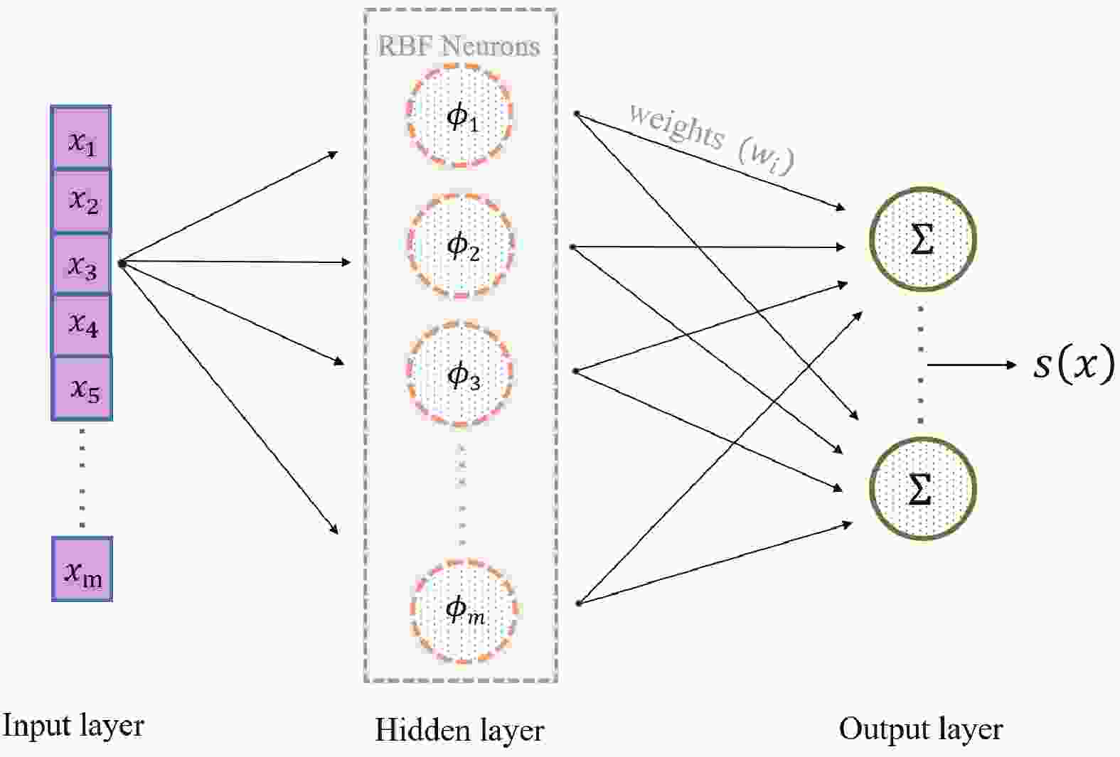
The general architecture of the RBFN method in the
$ \alpha $ decay calculation is shown in Fig. 1. In this approach, RBFs are used as activation functions of the form [40-42, 44-46]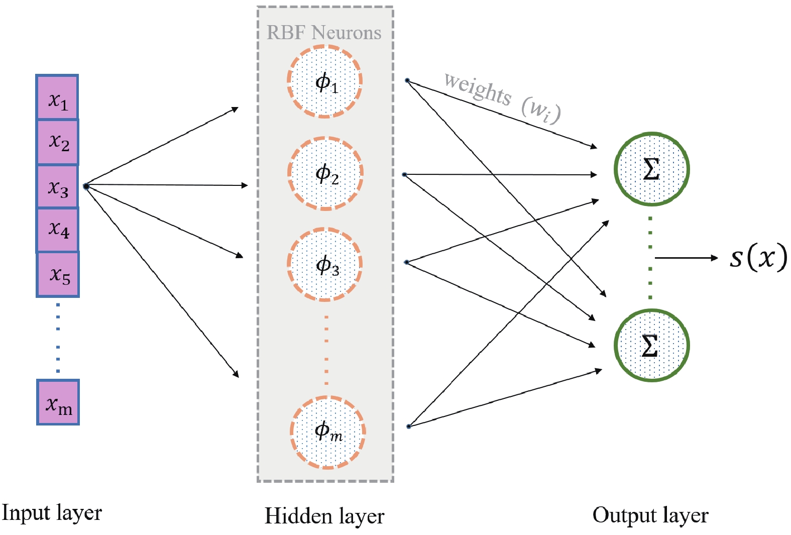
Figure 1. (color online) The architecture of the RBFN approach in α decay calculation.
$ S(x) = \sum\limits_{i = 1}^m {{\omega _i}} \phi (||x - {x_i}||),$

(6) where
$ S(x) $ is the reconstructed smooth function, and$ \phi(r) $ is the RBF. The network outputs a linear combination of RBFs of the inputs and neuron parameters. In addition, m represents the number of data points to be fitted,$ x_i $ is the measurement point, and$ \omega_i $ denotes the weight of the center of$ x_i $ , which is obtained by solving the matrix equation of$ \phi(r) $ and the deviation between the experimental half-life and the calculated data. By inserting$ \omega_i $ into Eq. (6), the corresponding smooth function$ S(x_i) $ can be obtained.With the help of the global interpolation and extrapolation of the RBFN method, the
$ \alpha $ decay half-life of an unmeasured nucleus can be predicted using experimental data. In other words, the half-life predictions for unmeasured nuclei can be treated as a problem of half-life surface extrapolation from the experimental data.The nuclei considered in our calculations, alongside the corresponding experimental data from Ref. [38], are shown in Fig. 2(a), where
$ 104\leqslant Z\leqslant 118 $ . To improve the accuracy of the half-life predictions more effectively, the 68 SHN were divided into four categories: even Z-even N, even Z-odd N, odd Z-even N, and odd Z-odd N. After considering the RBFN approach, the revised logarithm of$ \alpha $ decay half-life is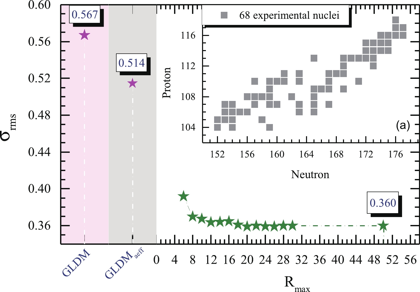
Figure 2. (color online) Distributions of 68 superheavy nuclei (a): the magenta stars denote the rms deviations of the half-life based on the GLDM with/without the surface diffuseness effect. The green stars describe the convergent behavior of the rms deviations in the RBFN approach.
$ {\rm{log}}_{10}T_{\rm{aeff}}^{\rm{RBFN}}(Z,N) = {\rm{log}}_{10}T_{\rm{aeff}}(Z,N)+S(Z,N). $

(7) Here,
$ {\rm{log}}_{10}T_{\rm{aeff}}(Z,N) $ denotes the result of the GLDM incorporating the diffuseness effect. -
There are several forms of the Euclidean norm
$ \phi(r) $ in the RBFN approach, such as Gaussian,$ \phi(r) = \exp^{-(\varepsilon r)^2} $ ; multiquadric,$ \phi(r) = 1+(\varepsilon r)^2 $ ; and inverse quadric,$ \phi(r) = \sqrt{1+(\varepsilon r)^2} $ . We tested possible forms of$ \phi(r) $ and found that an interesting phenomenon, namely$ \phi(r) = r $ , i.e.,$ ||x-x_i|| = \sqrt{(Z_i-Z_j)^2+(N_i-N_j)^2} $ , which stands for the distance between the nuclei$ (Z_i,N_i) $ and$ (Z_j,N_j) $ , yields a better prediction of the half-life than the aforementioned forms. This form is also suitable for the study of nuclear mass.The root-mean-square (rms) deviations with respect to the half-lives
$ (\sigma_{\rm{rms}})^2 = \frac{1}{n}\sum^n_{i = 1}|{\rm{log}}_{10}T_{1/2}^{\rm{Exp}}-{\rm{log}}_{10}T_{1/2}^{\rm{Cal}}|^2 $ were introduced to evaluate the precision of the theoretical calculations quantitatively. The$ \sigma_{\rm{rms}} $ corresponding to the GLDM with$ a_{\rm{eff}} $ fixed at 0.54 fm was 0.567. By introducing the semiempirical diffuseness formula [see Eq. (3)] into the GLDM, the rms deviations of half-life were reduced from 0.567 to 0.514, representing a reduction of up to 10%. Furthermore, the convergent behavior of the RBFN method was tested. It is worth pointing out that r is in the range of$ R_{\min}\leqslant r\leqslant R_{\max} $ . In Fig. 2, when$ R_{\max} = 0 $ , the reconstructed function$ S(Z,N) $ is zero. Thus,$ {\rm{log}}_{10}T_{\rm{aeff}}^{\rm{RBFN}}(Z,N) = {\rm{log}}_{10}T_{\rm{aeff}}(Z,N) $ , which means without the RBFN approach. Because we used 68 nuclei [see Fig. 2(a)], some of which are relatively scattered, an effective value of$ R_{\min} = 6 $ was used in this work. It is observed that the prediction accuracy converges at$ R_{\max}>20 $ for 68 SHN. The value of$ \sigma_{\rm{rms}} $ was reduced from 0.514 to 0.360, representing a total reduction of 40%. It should be noted that, for the GLDM, the calculated half-lives of most odd-X nuclei are worse than those of the even Z-even N nuclei, with the weight depending on the deviation in the RBFN approach. Hence, the$ \sigma_{\rm{rms}} $ value is only 0.538 when the GLDM and RBFN are combined without considering the surface diffuseness effect. Incorporating the surface diffuseness effect in the GLDM makes the description of most odd-X nuclei better in the${\rm{GLDM}} _{\rm{aeff}} $ . Therefore, the RBFN method can capture this effective information and optimize those nuclei with large deviations, which in turn improves the results of the RBFN.To determine how the odd-even property affects the surface diffuseness parameter and the RBFN approach, the rms deviations for the four aforementioned categories, even Z-even N, even Z-odd N, odd Z-even N, odd Z-odd N (e-e, e-o, o-e, o-o), are listed in Table 2. After including the surface diffuseness effect in the proximity energy for the GLDM, the
$ \sigma_{\rm{rms}} $ value reduces by a certain extent. Unfortunately, a slight systematic difference remains for the congeneric nuclei of even Z-odd N. This is because we performed the fitting scheme for 68 SHN simultaneously, and the sigma values for four the groups are the result of overall systematics. Thus, certain nuclei with large deviations between their experimental and theoretical half-lives, such as$ ^{267} $ Ds, cause the sigma value of e-o nuclei to exceed the results of the GLDM without the diffuseness effect. In addition, the GLDM is a semi-classical theoretical model, and the blocking effect of unpaired nucleons is not accounted for. Moreover, the sigma value is affected to a certain extent by the experimental half-life in the SHN region. Consequently, all models (GLDM,${\rm{GLDM}} _{\rm{aeff}} $ , and${\rm{GLDM}} _{\rm{aeff}}^{\rm{RBF}} $ ) can describe the alpha decay half-lives of o-e nuclei with greater accuracy than e-o nuclei. After implementing the RBFN approach, the obtained rms deviations for the four categories are approximately 16-50% less than non-RBFN-based calculations, indicating a considerable improvement for the half-life calculations.models $\sigma_{\rm{rms}}$ 

e-e e-o o-e o-o GLDM 0.272 0.510 0.350 0.794 ${\rm{GLDM}}_{\rm{aeff}}$ 

0.233 0.576 0.278 0.656 ${\rm{GLDM}}_{\rm{aeff}}^{\rm{RBFN}}$ 

0.201 0.421 0.270 0.412 Table 2. Comparison of the rms deviations for four categories, even Z-even N, even Z-odd N, odd Z-even N, and odd Z-odd N, using three models: GLDM, GLDM with the diffuseness effect in Eq. (3) (
${\rm{GLDM}}_{\rm{aeff}}$ ), and GLDM incorporating both the diffuseness effect and the RBFN approach (${\rm{GLDM}}_{\rm{aeff}}^{\rm{RBFN}}$ ).The
$ a_{\rm{eff}} $ values and the contributions from the RBFN approach for the 68 SHN are listed in Table 3. The corresponding deviations between the experimental half-life and the theoretical data, as well as the Gaussian statistical behavior (denoted by the blue dashed lines) are shown, respectively, in the top and bottom panels of Fig. 3. It is observed that an$ a_{\rm{eff}} $ reduction of approximately 0.1 fm can increase the value of$ {\rm{log}}_{10}T_{1/2} $ by 0.1 s. The values of$ a_{\rm{eff}} $ (seventh and fifteenth columns) match the diffuseness values in Ref. [37] (Table 1) and Ref. [38] (Table 1) closely. Three sets of$ a_{\rm{eff}} $ values show that the diffuseness values of odd-Z and/or odd-N nuclei are less than 0.54 fm. This indicates that, to some extent, including the odd-even effect in the surface diffuseness parameter is equivalent to incorporating the blocking effect of unpaired nucleons into the GLDM. Note that the half-lives calculated using the GLDM with the fixed value of$ a_{\rm{eff}} = 0.54 $ fm in the SHN region are systematically higher than those of the proxy model and the universal decay law in Ref. [61]. By incorporating the diffuseness effect, the changes to the surface behavior of the nucleus optimize the proximity energy, which in turn optimizes the potential barrier of reaction system, thereby improving the half-life calculation. It is worth pointing out that the semiempirical diffuseness formula (Eq. (15) in Ref. [38]) proposed by Nagib$ et\; al. $ does indeed improve the calculation of half-life, even though it does not work well in the GLDM framework. Together with the results shown in Fig. 3, we found that the surface diffuseness effect optimizes the calculation in comparison with the results produced using the conventional model, especially for nuclei whose GLDM-calculated half-lives were always higher than those recorded in the experimental data. Furthermore, the corresponding deviations between the experimental half-lives and the theoretical data in${\rm{GLDM}} _{\rm{aeff}} $ show a strong Gaussian distribution.nuclei $Q_\alpha^{\rm{Exp}}$ 

/MeV${\rm{log}}_{10}T_{1/2}{\rm {/s}}$ 

$a_{\rm{eff}}$ 

/fm$S$ /s

nuclei $Q_\alpha^{\rm{Exp}}$ 

/MeV${\rm{log} }_{10}T_{1/2}{\rm {/s} }$ 

$a_{\rm{eff}}$ 

/fm$S$ /s

Exp GLDM ${\rm{GLDM}}_{\rm{aeff}}$ 

${\rm{GLDM}}_{\rm{aeff}}^{\rm{RBFN}}$ 

Exp GLDM ${\rm{GLDM}}_{\rm{aeff}}$ 

${\rm{GLDM}}_{\rm{aeff}}^{\rm{RBFN}}$ 

$Z=104$ 

270Ds 11.120 −4.000 −3.656 −3.735 −3.912 0.573 −0.177 256Rf 8.926 0.319 0.227 0.165 0.079 0.562 −0.086 271Ds 10.899 −2.639 −2.452 −2.333 −2.506 0.424 −0.173 258Rf 9.190 −1.035 −0.686 −0.748 −0.707 0.564 0.041 273Ds 11.380 −3.770 −3.718 −3.605 −3.784 0.425 −0.179 263Rf 8.250 3.301 2.953 3.074 2.955 0.417 −0.119 277Ds 10.720 −2.222 −2.393 −2.283 −2.133 0.428 0.151 $Z=105$ 

281Ds 9.320 2.125 1.292 1.389 1.137 0.431 −0.252 257Db 9.206 0.389 0.696 0.635 0.826 0.413 0.191 $Z=111$ 

258Db 9.500 0.776 −0.570 −0.307 0.437 0.264 0.744 272Rg 11.197 −2.420 −3.494 −3.382 −1.976 0.274 1.406 259Db 9.620 −0.292 −0.629 −0.502 −0.513 0.414 −0.011 274Rg 11.480 −2.194 −4.147 −3.894 −3.048 0.276 0.846 263Db 8.830 1.798 1.498 1.621 1.823 0.417 0.202 278Rg 10.850 −2.377 −2.603 −2.349 −1.661 0.279 0.688 $Z=106$ 

279Rg 10.530 −1.046 −1.581 −1.473 −1.431 0.429 0.042 259Sg 9.804 −0.492 −0.692 −0.426 −0.934 0.414 −0.508 280Rg 9.910 0.663 −0.071 0.156 0.267 0.280 0.111 260Sg 9.901 −1.686 −1.878 −1.944 −2.056 0.565 −0.112 $Z=112$ 

261Sg 9.714 −0.638 −0.550 −0.424 −0.714 0.416 −0.290 281Cn 10.460 −1.000 −1.087 −0.855 −0.855 0.431 0.000 262Sg 9.600 −1.504 −1.128 −1.196 −1.228 0.567 −0.032 285Cn 9.320 1.447 1.977 2.072 2.003 0.434 −0.069 269Sg 8.700 2.079 2.075 2.188 2.253 0.422 0.065 $Z=113$ 

271Sg 8.670 2.219 2.070 2.182 2.356 0.424 0.174 278Nh 11.850 −3.620 −4.513 −4.401 −3.420 0.279 0.981 $Z=107$ 

282Nh 10.780 −1.155 −1.978 −1.742 −1.525 0.282 0.217 260Bh 10.400 −1.459 −2.543 −2.414 −1.260 0.265 1.154 283Nh 10.480 −1.000 −0.832 −0.733 −0.587 0.432 0.146 261Bh 10.500 −1.899 −2.181 −2.051 −2.016 0.416 0.035 284Nh 10.120 −0.041 −0.188 0.045 0.283 0.283 0.238 264Bh 9.960 −0.357 −1.324 −1.048 −0.701 0.268 0.347 285Nh 10.010 0.623 0.363 0.460 0.171 0.434 −0.289 266Bh 9.430 0.230 0.206 0.457 1.080 0.270 0.623 286Nh 9.790 0.978 0.808 1.042 0.900 0.285 −0.143 267Bh 9.230 1.230 0.970 1.085 1.295 0.420 0.210 $Z=114$ 

270Bh 9.060 1.785 1.420 1.674 1.952 0.273 0.278 286Fl 10.350 −0.699 −0.771 −0.674 −0.734 0.585 −0.060 272Bh 9.310 1.000 0.687 0.923 0.995 0.274 0.072 287Fl 10.170 −0.319 0.250 0.346 −0.264 0.435 −0.610 274Bh 8.930 1.732 1.865 2.102 2.152 0.276 0.050 288Fl 10.072 −0.180 −0.092 −0.179 −0.344 0.586 −0.165 $Z=108$ 

289Fl 9.980 0.279 0.672 0.760 0.079 0.437 −0.681 264Hs 10.591 −2.796 −2.973 −2.844 −2.869 0.568 −0.025 $Z=115$ 

265Hs 10.470 −2.699 −1.928 −1.808 −2.581 0.419 −0.773 287Mc 10.760 −1.432 −0.915 −1.008 −1.209 0.435 −0.201 266Hs 10.346 −2.638 −2.463 −2.534 −2.746 0.570 −0.212 288Mc 10.630 −1.060 −1.108 −0.889 −0.818 0.286 0.071 267Hs 10.037 −1.187 −0.906 −0.788 −1.151 0.420 −0.363 289Mc 10.520 −0.658 −0.406 −0.316 −0.544 0.437 −0.228 270Hs 9.050 0.556 1.084 1.010 0.715 0.573 −0.295 290Mc 10.410 −0.187 −0.482 −0.261 −0.465 0.287 −0.204 273Hs 9.730 −0.119 −0.410 −0.302 −0.293 0.425 0.009 $Z=116$ 

$Z=109$ 

290Lv 10.990 −1.824 −1.776 −1.686 −1.802 0.587 −0.116 268Mt 10.670 −1.678 −2.704 −2.584 −2.146 0.271 0.438 291Lv 10.890 −1.721 −1.064 −0.974 −1.683 0.438 −0.709 274Mt 10.200 −0.357 −1.409 −1.164 −0.658 0.276 0.506 292Lv 10.774 −1.745 −1.321 −1.415 −1.533 0.589 −0.118 275Mt 10.480 −1.699 −2.107 −1.997 −1.631 0.427 0.366 293Lv 10.680 −1.276 −0.621 −0.532 −1.223 0.440 −0.691 276Mt 10.030 −0.347 −0.907 −0.660 −0.559 0.277 0.101 $Z=117$ 

278Mt 9.580 0.653 0.418 0.664 0.754 0.279 0.090 293Ts 11.180 −1.854 −1.471 −1.567 −2.015 0.440 −0.448 $Z=110$ 

294Ts 11.070 −1.745 −1.764 −1.535 −1.368 0.290 0.167 267Ds 11.780 −5.553 −4.191 −3.922 −4.458 0.420 −0.536 $Z=118$ 

269Ds 11.509 −3.747 −3.724 −3.601 −4.495 0.422 −0.894 294Og 11.820 −3.161 −3.109 −3.018 −3.309 0.590 −0.291 Table 3. Calculations for 68 SHN. In order, the columns list the element, the corresponding experimental
$ Q_\alpha^{\rm{Exp}} $ , the logarithm of the experimentally-measured half-lives, the GLDM,${\rm{GLDM}} _{\rm{aeff}} $ , and${\rm{GLDM}} _{\rm{aeff}}^{\rm{RBFN}} $ predictions, the$ a_{\rm{eff}} $ value, and the S value. The right half of the Table is the same as the left half.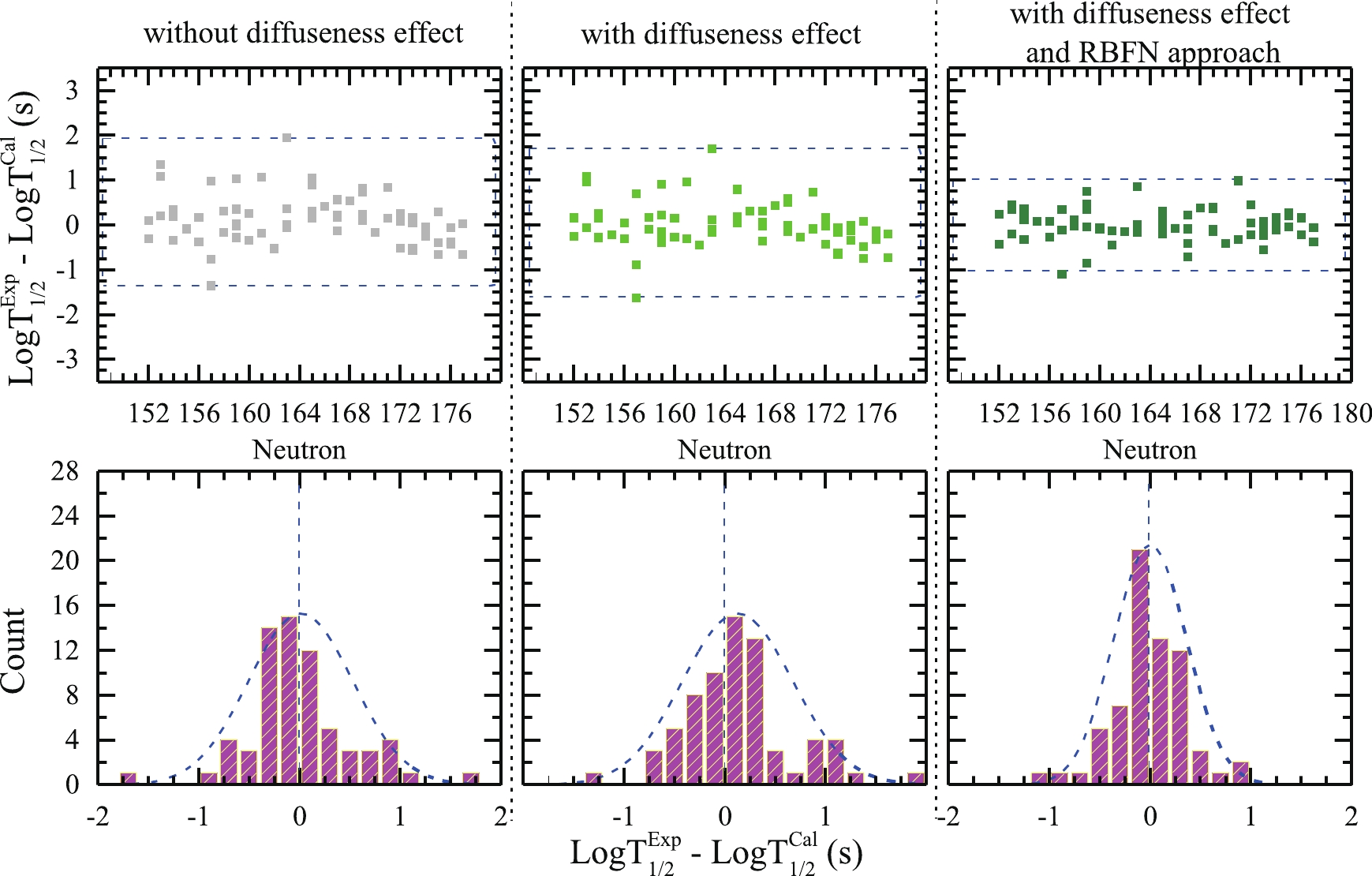
Figure 3. (color online) Top panel: differences between the experimental and calculated
$\alpha$ decay half-lives for 68 SHN. Bottom panel: histograms of these differences for the GLDM,${\rm{GLDM}}_{\rm{aeff}}$ , and${\rm{GLDM}}_{\rm{aeff}}^{\rm{RBFN}}$ . The blue dashed lines denote the corresponding Gaussian distributions.In addition, the RBFN approach results in a remarkable improvement in the half-life calculation accuracy; the differences are populated almost exclusively between 1 and -1 and are systematically smaller than those corresponding to the GLDM with/without surface diffuseness effect, as shown in Fig. 3. The corresponding reconstructed functions
$ S(Z,N) $ are presented in Table 3. One can find that an inseparable connection exists between the$ S(Z,N) $ of the RBFN correction and the deviations between the experimental half-life and the theoretical data in the${\rm{GLDM}} _{\rm{aeff}} $ . As the weight$ \omega_i $ determines the value of the reconstructed function$ S(x_i) $ according to the deviation, relatively large deviations between the theoretical calculations and experimental data can be compensated using the RBFN approach, especially for$ ^{260} $ Bh,$ ^{265} $ Hs,$ ^{268,274} $ Mt,$ ^{272,274} $ Rg,$ ^{278} $ Nh, and$ ^{291,293} $ Lv. Taking$ ^{260} $ Bh as an example, the$ {\rm{log}}_{10}T_{1/2} $ value changes from -2.543 s in the conventional GLDM to -1.26 s when both the diffuseness and RBFN corrections are applied, representing an increase of more than 50%. More interestingly, we found that such deviation reductions are not a monotonic improvement; most of the theoretical half-lives are getting closer to the corresponding experimental values irrespective of whether the theoretical value is larger or smaller than the experimental value. This result reveals that the surface diffuseness effect plays an important role in the theoretical description of$ \alpha $ decay. Therefore, we can confirm that the RBFN approach is a powerful tool for optimizing decay calculations. -
Several theoretical works suggest the possibility of doubly magic nuclei beyond
$ ^{280} $ Pb, for example,$ ^{298} $ Fl in the macroscopic-microscopic approach [62],$ ^{304} $ 120 in the relativistic Hartree-Fock-Bogoliubov (RHFB) theory [63], and$ Z = 124 $ or 126, with$ N = 184 $ in the nonrelativistic Skyrme-Hartree-Fock models. In addition, following the synthesis of$ ^{294} $ Og SHN, there have been attempts to produce nuclei with$ Z = 119 $ and 120 [5-12, 16]. The$ \alpha $ decay process is one of main decay modes in SHN. Encouraged by the above improvements produced by the RBFN approach and surface diffuseness effect, we predicted the half-lives of four isotopes: 252-288Rf, 272-310Fl, 286-316119, and 292-318120. It is well known that half-lives are extremely sensitive to the decay energy and the barrier potential. Figure 4 shows the variation in the decay energy and the calculated half-life for different isotopic chains. Here, the decay energies$ Q_\alpha^{\rm{WS4}} $ (denoted by blue squares) from the WS4 model [64] and$ Q_\alpha^{\rm{FRDM}} $ values (red circles) from the FRDM model [65] were used as inputs.
Figure 4. (color online) The
$ \alpha $ decay energies$ Q_\alpha $ from the WS4 [64] and FRDM [65] models are denoted by blue squares and red circles, respectively, in the left-hand side of the subfigures. The$ \alpha $ decay half-lives calculated using the${\rm{GLDM}} _{\rm{aeff}} $ and${\rm{GLDM}} _{\rm{aeff}}^{\rm{RBFN}} $ for isotopes with$ Z = $ 104, 114, 119, and 120 (even-N numbers only) are shown in the right-hand side of the subfigures.The
$ Q_\alpha $ values and the corresponding$ {\rm{log}}_{10}T_{1/2} $ data show symmetrically opposite trends, especially for the 252-288Rf isotope. This is consistent with the Geiger-Nuttall law,$ {\rm{log}}_{10}T_{1/2} = a\dfrac{1}{\sqrt{Q_\alpha}}+b $ . It is well known that the half-life is extremely sensitive to the$ Q_\alpha $ value. When a large discrepancy appears for the$ Q_\alpha $ value between the WS4 and FRDM models, it is reflected in the half-lives. For instance, a deviation of 1 MeV between$ Q_\alpha^{\rm{WS4}} $ and$ Q_\alpha^{\rm{FRDM}} $ leads to a$ {\rm{log}}_{10}T_{1/2} $ difference of approximately$ 10^4 $ for the$ ^{282} $ Fl nucleus. By contrast, the calculated$ \alpha $ decay half-lives that have been improved by the surface diffuseness effect and the RBFN approach both increase as the neutron number increases up to a possible neutron magic number and then decrease with the neutron number up to the possible neutron magic (or submagic) number plus two. After that, they increase again. It is well known that$ \alpha $ radioactivity shell effects are related to the$ Q_\alpha $ , which peaks when the daughter nuclei have a magic number of neutrons and protons. Therefore, the two sets of decay energy,$ Q_\alpha^{\rm{WS4}} $ and$ Q_\alpha^{\rm{FRDM}} $ , exhibit the opposite trend to the half-life. Both the decay energy and half-life reflect the strong shell effects at$ N = 184 $ , which confirms that the next neutron magic number after$ N = 126 $ is$ N = 184 $ . Furthermore,$ N = 152, \; 162 $ , and 178 are possible candidates for neutron submagic numbers. In addition,$ N = 196 $ emerges as a possible neutron submagic number from the WS4$ Q_\alpha $ decay energy and the corresponding half-lives of the$ Z = 119 $ and 120 isotopes. Moreover, the values of$ Q_\alpha $ and$ {\rm{log}}_{10}T_{1/2} $ show little change from$ N = 178 $ to 184. This indicates that the nuclei in this region are relatively stable. -
In summary, we incorporated the surface diffuseness effect into the proximity energy by expressing the diffuseness in terms of the sharp radius effect and an odd-even correction to improve
$ \alpha $ decay calculations. Meanwhile, the RBFN method is applied to$ \alpha $ decay calculations for the first time. The rms deviations of 68 SHN in the GLDM framework fell from 0.567 to 0.360, representing a reduction of up to 40%. Then, we extrapolated the half-lives of 252-288Rf, 272-310Fl, 286-316119, and 292-318120 isotopes using WS4 and FRDM$ Q_\alpha $ values as inputs. Our primary conclusions can be summarized as two points:(i) The calculated
$ \alpha $ decay half-lives reproduced the experimental data with high accuracy by considering the RBFN method via the improved GLDM incorporating the diffuseness effect. Therefore, we conclude that the diffuseness effect is an important physical effect that should be introduced into the calculations of$ \alpha $ decay and spontaneous fission. Furthermore, we encourage the widespread use of the RBFN method in nuclear reaction studies.(ii) Both the decay energies and half-lives of the 252-288Rf, 272-310Fl, 286-316119, and 292-318120 isotopes indicate that
$ N = 184 $ is a neutron magic number candidate, while$ N = 152,162,178 $ are neutron submagic numbers. In addition,$ N = 196 $ is a possible neutron submagic number based on the WS4$ Q_\alpha $ decay energy and corresponding half-life.
Diffuseness effect and radial basis function network for optimizing α decay calculations
- Received Date: 2020-08-20
- Available Online: 2021-02-15
Abstract: A radial basis function network (RBFN) approach is adopted for the first time to optimize the calculation of


 DownLoad: