


 Abstract
 HTML
HTML Reference
 Related
 PDF
PDF


-
Recently, the XENON collaboration reported a new result regarding the low energy electron recoil data in the Science Run 1 (SR1) data collected by the Xenon1T experiment from February 2017 to February 2018, with an exposure of 0.65 tonne-years: 285 events were observed in the electron recoil energy between 1 keV and 7 keV, while the background expectation was
$ 232 \pm 15 $ events [1]. Various backgrounds for the excess events have been studied by the XENON collaboration [1]. The uncertainty in the Pb-214 background was not found to be sufficiently large to explain the excess [1]. Although the$ \beta $ emission of tritium is a good fit to the excess data, the amount of tritium resulting from cosmogenic activation is found to be much smaller than needed for the excess [1]. However, there could be some other sources of tritium inside the Xenon1T detector.Some new physics explanations have also been investigated by the XENON collaboration [1]. Axions produced from the Sun and neutrinos with a magnetic moment have been found to be a good fit to the excess events, with significances of 3.5
$ \sigma $ and 3.2$ \sigma $ , respectively [1]. However, the solar axion explanation is in strong tension with the stellar cooling constraint [2-5], and neutrinos with a magnetic moment are also constrained [1]. Axion-like particles [6] and dark matter (DM) particles with very large velocity [7] have been proposed recently to explain the excess data. A possible excess signal in the electron recoil has also been studied recently [8].In this paper, we present a DM explanation of the excess events in the Xenon1T low energy electron recoil data. In our model, DM particle
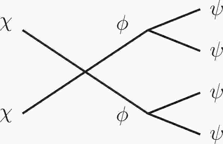
$ \chi $ annihilates into a pair of on-shell particles$ \phi $ that subsequently decay into the$ \psi \psi $ final state; the decay diagram is shown in Fig. 1. We refer to this model as the on-shell mediator dark matter model (see e.g., [9-14] for early studies). We assume that$ \psi $ has a sizeable interaction cross section with electrons. The produced$ \psi $ particle can have a rather large velocity, leading to a$ \sim $ keV electron recoil energy recorded by the Xenon1T detector.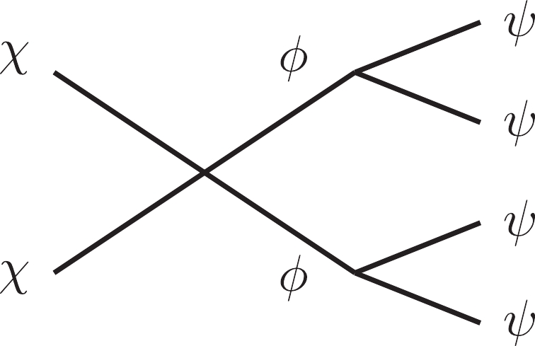
Figure 1. Decay diagram of the on-shell mediator model.
We show that the
$ \psi $ particle can have an extended velocity distribution because of the mass hierarchy, which provides a good fit to the excess spectrum in the Xenon1T electron recoil data. We further estimate the flux of$ \psi $ and the interaction cross section with electrons. We find that the flux of$ \psi $ is consistent with the expectation from DM annihilation in the galaxy, and the interaction cross section required for the excess is sufficiently small such that$ \psi $ is not stopped by the rocks on top of the underground labs. -
We consider a hidden sector that contains three particles:
$ \chi $ (the DM particle),$ \phi $ (the mediator), and$ \psi $ . The interaction between$ \psi $ and electrons gives rise to electron recoil signals in the Xenon1T detector.$ \psi $ is assumed to be either stable or long-lived but with a negligible relic abundance. We assume the following mass hierarchy,$ m_\chi > m_\phi > 2 m_\psi $ , so that DM$ \chi $ can annihilate in the following manner$ \chi \chi \to \phi \phi \to \psi \psi \psi \psi. $

(1) Assuming
$ \psi $ is isotropically produced in the rest frame of$ \phi $ , the energy spectrum of the$ \psi $ particle has a box-shape distribution in the energy range$ E_{-} < E_\psi < E_{+}, $

(2) where
$ E_{\pm} = (m_\chi / 2) (1\pm x y) $ , with$ x = \sqrt{1-{m_\phi^2 / m_\chi^2}} $ and$ y = \sqrt{1-{4 m_\psi^2 / m_\phi^2}} $ . This leads to a velocity distribution of$ \psi $ as follows:$ \begin{aligned}[b] \int_{v_{-}}^{v_{+}} {\rm d}v_\psi f(v_\psi) =& \int_{v_{-}}^{v_{+}} \frac{{\rm d}v_\psi\, v_\psi\, m_{\psi}}{(E_{+}-E_{-})(1-v_\psi^{2})^{3 / 2}} \\ =& \int_{v_{-}}^{v_{+}} {\rm d}v_\psi \frac{ v_\psi \sqrt{1-x^2} \sqrt{1-y^2} }{2\, (1-v_\psi^{2})^{3/2}\, x\, y }, \end{aligned} $

(3) where
$ v_\psi(E_\psi) = \sqrt{1-m_\psi^2/E_\psi^2} $ is the velocity of$ \psi $ , and$ v_{\pm} = v_\psi(E_{\pm}) = |x\pm y|/(1\pm x y) $ . We note that both$ v_{\pm} $ and$ f(v_\psi) $ are invariant when x and y are interchanged. Fig. 2 shows the velocity distribution$ f(v_\psi) $ for the three benchmark models listed in Table 1: (x, y) = (0.504, 0.0945) for model A, (x, y) = (0.117, 0.0321) for model B, and (x, y) = (0.0856, 0.00197) for model C. Because the velocity distributions for the on-shell mediator models are very different from the Maxwell-Boltzmann distribution for canonical DM particles, the electron recoil energy resulting from the$ \psi $ -electron interaction can be much higher.Model $ m_{\psi} $ /keV

x y $ n_{\psi} \bar{\sigma}_{{\rm{e}} \psi} $ /(cm−1)

A 50 0.504 0.0945 $ 13.3 \times 10^{-43.5} $ 

B $ 10^3 $ 

0.117 0.0321 $ 1.58 \times 10^{-43.5} $ 

C $ 10^6 $ 

0.0856 0.00197 $ 1.17 \times 10^{-43.5} $ 

Table 1. Benchmark model points.
$ n_{\psi} \bar{\sigma}_{{\rm{e}} \psi} $ is the best-fit value to interpret the Xenon1T excess events.
Figure 2. (color online) Velocity distributions of the particle
$ \psi $ for the three benchmark models in Table 1. -
The differential rate caused by scattering between
$ \psi $ and electrons can be computed by [15-18]$ \frac{ {\rm d} \langle \sigma v_\psi \rangle}{{\rm d}E_R} = \frac{\bar{\sigma}_{e\psi}} {2 m_e} \int \frac{{\rm d}v_\psi f(v_\psi)}{v_\psi} \int_{q_{-}}^{q_{+}} a_0^2 q {\rm d} q |F (q)|^2 K(E_R,q), $

(4) where
$ f(v_\psi) $ is the$ \psi $ velocity distribution given in Eq. (3);$ F (q) $ is the dark matter form factor, which is assumed to be unity in this analysis;$ E_R $ is the electron recoil energy;$ K(E_R,q) $ is the dimensionless atomic excitation factor [17-19]; and$ \bar{\sigma}_{e\psi} $ is the free electron cross section at a fixed momentum transfer of$ q = 1/a_0 $ , with$ a_0 = 1/(m_e \alpha) $ the Bohr radius. For simplicity, in our analysis, we assume that the cross section$ \sigma_{e \psi} $ is independent of the momentum transfer q. Here, we only consider the contributions from the$ n = 3,4,5 $ electrons in Xenon. As demonstrated in the appendix, the$ n = 1,2 $ electrons do not give significant contributions to the Xenon1T electron recoil spectrum, at least for the benchmark model points shown in Fig. 3.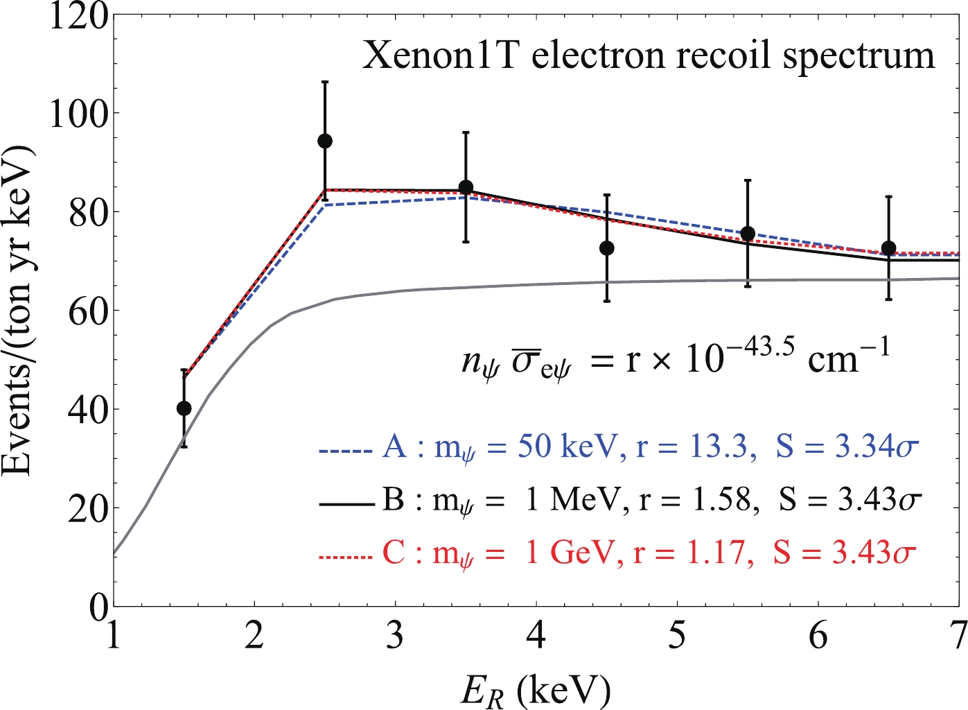
The integration limits on the momentum transfer are given by [15, 16, 18]
$ q_{\pm} = m_\psi v_\psi \pm \sqrt{m_\psi^2 v_\psi^2 - 2 m_\psi E_R}. $

(5) The differential event rate then can be obtained as
$ \frac{{\rm d}R}{{\rm d}E_R} = N_T n_\psi \frac{{\rm d} \langle \sigma v_\psi \rangle}{{\rm d}E_R}, $

(6) where
$ N_T $ is the number of atoms in the target material, and$ n_\psi $ is the number density of the incident$ \psi $ particle. We take$ N_T \simeq 4.2 \times10^{27} \,{\rm{ton}}^{-1} $ for Xenon atoms.We further smear the differential event rate in Eq. (6) using a Gaussian distribution with an energy resolution of
$ 0.45 $ keV [20]. The number of events is then calculated as$ N_{S} = {\rm{exposure}}\int_{E_1}^{E_2} {\rm d}E_R \frac{{\rm d}R}{{\rm d}E_R} \epsilon (E_R), $

(7) where the exposure is 0.65 tonne-years, and
$ \epsilon (E_R) $ is the total efficiency of the Xenon1T experiment [1]. -
We use the on-shell mediator models to fit the excess events in the Xenon1T electron recoil energy range 1-7 keV in Fig. 3. We take the background from the Xenon1T paper [1]. The on-shell mediator models have four independent parameters:
$ m_\psi $ , x, y, and$ n_\psi \bar\sigma_{e \psi} $ . We consider three benchmark model points on Fig. 3:$ (m_\psi, x, y) = (50 $ keV, 0.504, 0.0945) for model A,$ (m_\psi, x, y) = (1 $ MeV, 0.117, 0.0321) for model B, and$ (m_\psi, x, y) = (1 $ GeV, 0.0856, 0.00197) for model C.We carry out a simple chi-squared analysis by taking into account only the six low energy electron recoil data points shown in Fig. 3;
$ \chi^2 $ is calculated as$ \chi^2 = \sum\limits_i \frac{(N^i_{\rm{exp}} - N^i_{\rm{th}})^2}{(\delta N^i_{\rm{exp}})^2}, $

(8) where i denotes the bins,
$ N^i_{\rm{exp}} $ and$ \delta N^i_{\rm{exp}} $ are the number of observed events and its uncertainty taken from Xenon1T, respectively [1].$ N^i_{\rm{th}} $ is the number of signal events calculated in Eq. (7) plus the expected background (integrated within the bin) taken from Xenon1T [1].The product of the number density of
$ \psi $ and its interaction cross section with the electron,$ n_\psi \bar \sigma_{e \psi} $ , is determined by minimizing$ \chi^2 $ for the benchmark model points in Fig. 3. Only using the background,$ \chi^2 \simeq 13.5 $ , which is shown as the gray line in Fig. 3 to fit the spectrum. We have$ \chi^2 \simeq 2.33 $ ,$ 1.71 $ , and$ 1.66 $ for the benchmark model points A, B, and C, respectively, using both the background and the new physics signal to fit the spectrum. This leads to a significance of$ \sim $ 3.43$ \sigma $ for the benchmark model points B and C and a significance of$ \sim $ 3.34$ \sigma $ for the benchmark model point A in Fig. 3. -
The parameter space of the model is spanned by four quantities:
$ m_\psi $ , x, y, and$ n_\psi \bar\sigma_{e \psi} $ . Because the signal events depend linearly on$ n_\psi \bar\sigma_{e \psi} $ , we always fix the$ n_\psi \bar\sigma_{e \psi} $ value by minimizing the$ \chi^2 $ fit to the Xenon1T data points shown in Fig. 3. We further define two velocity quantities,$ \bar{v} = (v_{+} + v_{-})/2 $ and$ \Delta v = v_{+} - v_{-} $ , which are functions of x and y only. Here,$ \bar{v} $ is the “average” velocity, and$ \Delta v $ is the width of the velocity distribution. Thus, we carry out scans in the three dimensional parameter space spanned by$ m_\psi $ ,$ \bar{v} $ , and$ \Delta v $ . The best-fit model point found in our three dimensional scans is ($ m_\psi $ ,$ \bar{v} $ ,$ \Delta v $ ) = ($ 117.5 $ MeV,$ 0.086 $ ,$ 0.011 $ ), with$ \chi^2_{\rm{min}} = {1.656} $ , which corresponds to$ n_\psi \bar\sigma_{e \psi} = 3.73\times 10^{-44} $ cm−1.We further carry out scans in the two dimensional space spanned by
$ \bar{v} $ and$ \Delta v $ , while the$ m_\psi $ value is kept fixed. Fig. 4 shows the 1$ \sigma $ regions corresponding to$ \Delta \chi^2 = \chi^2 - \chi^2_{\rm{min}} \leqslant 2.3 $ with$ \chi^2_{\rm{min}} = {1.656} $ , in the$ \bar{v}-\Delta v $ plane for$ m_\psi = 50 $ keV,$ m_\psi = 1 $ MeV, and$ m_\psi > {\cal O} (100) $ MeV. As shown in Fig. 4, the preferred average velocity$ \bar v $ increases when$ m_\psi $ decreases. In particular, in the 1$ \sigma $ region, we have$ 0.03 \lesssim \bar v \lesssim 0.3 $ for$ m_\psi \gtrsim 100 $ MeV,$ 0.07 \lesssim \bar v \lesssim 0.3 $ for$ m_\psi = 1 $ MeV, and$ 0.3 \lesssim \bar v \lesssim 0.7 $ for$ m_\psi = 50 $ keV. We also found that the 1$ \sigma $ regions extend to the$ \Delta v \to 0 $ case and become larger as$ \Delta v $ increases.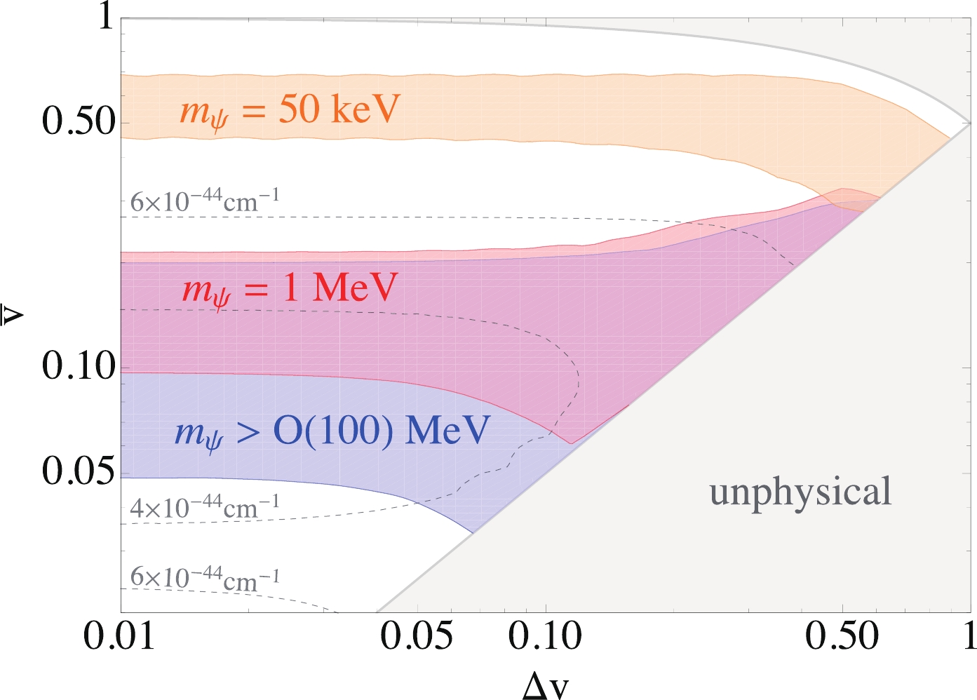
Figure 4. (color online)
$ 1\sigma $ region for fitting Xenon1T data in the$ \bar{v}-\Delta v $ plane for$ m_\psi =50 $ keV (orange), for$ m_\psi =1 $ MeV (red), and for$ m_\psi > {\cal O} (100) $ MeV (blue). The gray dashed contours indicate the$ n_\psi \sigma_{e \psi} $ value in units of cm$ ^{-1} $ for each model point at$ m_\psi = 100 $ MeV, which is obtained by minimizing the$ \chi^2 $ fit to the data. The gray shaded region is the unphysical region where$ v_{-} < 0 $ or$ v_{+} > 1 $ .We note that for the heavy mass region,
$ m_\psi \gtrsim 100 $ MeV, the signal becomes insensitive to$ m_\psi $ . This is because for$ m_\psi \gtrsim 100 $ MeV, the lower and upper limits of the integration in Eq. (4) become$ q_{-} \simeq E_R / v_\psi $ and$ q_{+} \simeq 2 m_\psi v_\psi $ . Because the kernel function K falls rapidly as q increases to large values, for the heavy$ \psi $ mass case, the integration over q in Eq. (4) is only determined by the lower limit of the integration,$ q_{-} \simeq E_R / v_\psi $ , which is independent of$ m_\psi $ . -
To compute the flux of
$ \psi $ from DM annihilations, we assume an NFW profile for the Milky Way DM halo$ \rho_\chi(r) = \rho_{s} \frac{\left(r / r_{s}\right)^{-\gamma}}{\left(1+r / r_{s}\right)^{3-\gamma}}, $

(9) where we take
$ \gamma = 1 $ ,$ \rho_{s} = 0.31 $ GeV/cm3, and$ r_{s} = 21 $ kpc. The flux of$ \psi $ is given by$ \Phi_{\psi} = 4 \frac{\langle\sigma v\rangle}{8 \pi m_{\chi}^{2}} J, $

(10) where we have assumed that
$ \psi $ is self-adjoint, the total J-factor is$J = \int {\rm d} \Omega \int {\rm d} s \rho_{\chi}^{2} \simeq 10^{23}$ $ {\rm{GeV^2/cm^5}} $ , and$ \langle\sigma v\rangle $ is the DM annihilation cross section. The total$ \psi $ flux is$ \Phi_{\psi} \simeq 10^{-4} $ ($ 10^{2} $ ) cm−2 s−1 for$ m_{\psi} \simeq $ GeV (MeV) if the canonical thermal cross section$ \langle\sigma v\rangle = 3\times 10^{-26}\ {\rm{cm^3/s}} $ is assumed.① We note that the particle flux of$ \psi $ can be further enhanced if there exist some DM subhalos in the vicinity of the solar system.Using the benchmark model point C on Fig. 3, we determine the interaction cross section to be
$ \sigma_{e \psi} \simeq 6 \times 10^{-31} $ cm2. This is much larger than the dark matter direct detection upper limit of$ \sigma_{\rm{e-DM}} \lesssim10^{-38} $ cm2 [21]. However, the particle flux of$ \psi $ is approximately eight orders of magnitude smaller than the local DM flux,$ \Phi_{\chi} \simeq $ 105 cm-2 s-1 for$ m_\chi \simeq $ GeV. Thus,$ \psi $ with$ \sigma_{e \psi} \simeq 6 \times 10^{-31} $ cm2 is allowed under the DM direct detection limits.However, if the interaction cross section between
$ \psi $ and electrons is very large,$ \psi $ can be absorbed by the rocks on top of the underground labs. Ref. [22] shows that$ \psi $ is stopped by the interaction with rocks on top of a 2 km deep underground lab if$ \sigma_{e \psi} \gtrsim 10^{-24} $ cm2 for$ m_\psi \simeq {\cal O} $ (MeV), and the required cross section to stop$ \psi $ increases significantly with the$ \psi $ mass. For the benchmark model points A and B in Fig. 3, the required cross sections are$ \sigma_{e \psi} \simeq 10^{-37} $ and$ 10^{-36} $ cm2, respectively, which are much smaller than that of the benchmark model point C. Thus, for the benchmark model points in Fig. 3, the$ \psi $ particle can penetrate the rocks to enter the Xenon1T underground lab. -
A possible realization of the on-shell mediator model discussed is a hidden sector model in which
$ \chi $ and$ \psi $ are fermions charged under the hidden$ U(1) $ gauge boson$ \phi = \phi_\mu $ . Both$ \chi $ and$ \psi $ are stable because of the hidden$ U(1) $ gauge symmetry. The interaction Lagrangian in the hidden sector is given by$ g_h \phi_\mu (\bar \chi \gamma^\mu \chi + \bar \psi \gamma^\mu \psi). $

(11) The particle
$ \psi $ can either interact with an electron via some electrophilic interaction or interact with the standard model fermions via another gauge boson$ A'_\mu $ , which is kinetically mixed with the standard model hypercharge boson.We note that such models can be searched for in
$ e^+e^- $ colliders. For example, LEP data place constraints on the interaction between$ \psi $ and electrons via the mono-photon plus a large missing energy channel [23]. If we assume a four-fermion interaction operator$ (1/\Lambda^2)\bar \psi \psi \bar e e $ , the LEP lower bound$ \Lambda \gtrsim 440 $ GeV [23] leads to an upper limit$ \bar{\sigma}_{e \psi} \lesssim 1 \times 10^{-45} \,{{\rm{cm}}^2} $ , which is many orders of magnitude lower than the$ \bar{\sigma}_{e \psi} $ value required for the Xenon1T excess for GeV$ \psi $ mass. Although the direct detection process can be enhanced relative to the collider process, one simple way to avoid the LEP constraints is to assume a heavy$ \psi $ mass,$ m_\psi \gtrsim 100 $ GeV. Because$ \Phi_{\psi} $ in the$ m_\psi = 100 $ GeV case is approximately$ 10^4 $ times smaller than in the$ m_\psi = 1 $ GeV case, as in the benchmark model point C in Fig. 3, the preferred cross section is$ \bar{\sigma}_{e \psi} \sim {\cal O} (10^{-24}) $ cm2, where the difference between the annihilation cross section in the galaxy and in the early universe is also taken into account. For such a large cross section with an electron, the interaction with rocks decreases the kinetic energy of$ \psi $ significantly, such that the$ \psi $ particles in the Xenon1T lab are no longer sufficiently energetic to produce the excess electron recoil events. One way to address this is to assume a much larger DM annihilation cross section than the canonical value,②$ 3 \times 10^{-26} $ cm3/s, so that$ \bar{\sigma}_{e \psi} $ is significantly smaller than$ {\cal O} (10^{-24}) $ cm2.If
$ m_\chi > m_{\phi_\mu} $ the contribution to the DM annihilation cross section is dominated by the$ \chi \chi \to \phi_\mu \phi_\mu $ process. We followed the calculations in Ref. [12] to compute the relic density of DM$ \chi $ in the thermal freeze out scenario via the annihilation process$ \chi \chi \to \phi_\mu \phi_\mu $ . We found that to produce the correct amount of DM, one needs$ g_h \simeq 0.03 $ for$ m_\chi \simeq $ 1 GeV; for lighter mass,$ \lesssim $ GeV, the required$ g_h $ value is smaller.The mass hierarchy
$ m_\chi > m_\phi > 2 m_\psi $ leads to the box-shaped energy spectrum of$ \psi $ . If$ m_\phi > m_\chi $ the annihilation process$ \chi\chi \to \phi \to \psi\psi $ dominates; the energy spectrum of$ \psi $ is a delta function, smeared by the small kinetic energy of DM$ \chi $ . The velocity distribution in the$ \chi\chi \to \phi \to \psi\psi $ case has been investigated in Ref. [7]. -
We have analyzed the on-shell mediator DM models to fit the excess events in the low energy electron recoil data observed by Xenon1T. The on-shell mediator DM models can provide a good fit to the Xenon1T data; for example, a significance of 3.43
$ \sigma $ is achieved with$ n_\psi \sigma_{e\psi} \simeq {\cal O} (10^{-43.5}) $ cm-1 for$ m_\psi \simeq {\cal O} $ (GeV). The Xenon1T electron recoil excess events are insensitive to the width of the velocity distribution$ \Delta v $ ; perhaps more data accumulated in the future could improve the sensitivity to$ \Delta v $ .The electron recoil signals are somewhat independent of
$ m_\psi $ if$ m_\psi > {\cal O} (100) $ MeV. The preferred average velocity is$ 0.03 \lesssim \bar v \lesssim 0.3 $ for heavy$ \psi $ mass in the mass range$ m_\psi \gtrsim 100 $ MeV; for light$ \psi $ mass,$ 0.3 \lesssim \bar v \lesssim 0.7 $ for$ m_\psi = 50 $ keV. The benchmark models that can explain the Xenon1T excess are consistent with the expected flux arising from the DM annihilations in the Milky Way DM halo. Although the interaction cross section required for the excess is sizable, e.g.,$ \sigma_{e \psi} \simeq 10^{-31} $ cm2 for$ m_\psi \simeq {\cal O} $ (GeV), it is sufficiently small so that$ \psi $ can penetrate the rocks to reach the underground labs.Note added.− After the submission of the first version of our paper to arXiv, many papers attempting to interpret the Xenon1T excess [24-37] appeared on arXiv on the same day as our paper, or a day before.
-
We thank Yue Ma and Juri Smirnov for discussion and correspondence. V.Q. would like to thank the Institute of Physics, Academia Sinica, for its hospitality during this work.
-
In this appendix, we demonstrate that for our benchmark model points, the contributions from the
$ K $ -shell and$ L $ -shell electrons are negligible, compared with the contributions from the$ n = 3,4,5 $ electrons in Xenon. In our analysis, we adopt the recent computations of the atomic form factor [17-19], where relativistic corrections have been taken into account. In this appendix, however, we use the tabulated Roothaan-Hartree-Fock (RHF) functions [38] to compute the Xenon atomic form factor, in which one can easily include or exclude electrons from different orbits.We parameterize the differential cross section as in Refs. [15, 39],
$\tag{A1} \frac{ {\rm d} \langle \sigma v\rangle}{{\rm d} \ln E'} = \frac{\bar{\sigma}_{e \psi}} {8 \mu^2_{e \psi}} \int \frac{{\rm d}v f(v)}{v} \int_{q_{-}}^{q_{+}} q{\rm d}q |f_{\rm{ion}}^i (k',q) |^2 \,|F_D^\mu (q)|^2, $

where
$ \mu_{e \psi} = m_\psi m_e/(m_\psi +m_e) $ is the reduced mass,$ k' $ is the outgoing electron momentum, and$ E' $ is the energy of the outgoing electron, which is given by$E' = k'^2/(2m_e) = $ $ E_R - E_{n \ell} $ with$ E_R $ being the total energy deposited and$ E_{n\ell} $ being the binding energy of the$ (n\ell) $ electron of Xenon, as given in Table A1. Using the RHF function [38] for the initial bound-state electron and taking the plane wave approximation for the final state electron, the form factor for ionization,$ f_{\rm{ion}}^i (k',q) $ , is given by [39],Orbital $1{s}$ 

$2{s}$ 

$2{p}$ 

$3{s}$ 

$3{p}$ 

$3d$ 

$4s$ 

$4p$ 

$4d$ 

$5s$ 

$5p$ 

$E_{n\ell}$ /keV

34.561 5.453 5.107 1.1487 1.0021 0.689 0.2132 0.1467 0.0695 0.0695 0.0134 $Z_{\rm{eff}}$ 

52.9 39.8 49.8 35.6 35.7 39.9 26.2 25.0 21.9 14.2 12.4 $ \tag{A2}\begin{aligned}[b] |f_{\rm{ion}}^i (k',q) |^2 =& F_{\rm{fermi}} (E_R, Z_{\rm{eff}}) \frac{(2 \ell+1) k'^2}{4\pi^3 q} \\ &\times \int_{|k'+q|}^{|k'-q|} k {\rm d}k |\chi_{n\ell} (k)|^2, \end{aligned} $

where the Fermi factor is given by
$\tag{A3} F_{\rm{fermi}} (E_R, Z_{\rm{eff}}) = \frac{2 \pi \xi} {(1- {\rm e}^{-2 \pi \xi})}, $

where
$ \xi = \alpha Z_{\rm{eff}}\sqrt{m_e/(2 E_R)} $ . The effective Z values,$ Z_{\rm{eff}} $ , are listed in Table A1, adopted from Refs. [41, 42]. The momentum space radial wave function$ \chi_{n\ell} (k) $ is given by [43],$\tag{A4} \chi_{n\ell} (k) = 4 \pi i^{\ell} \int {\rm d} r r^2 R_{n \ell}(r) j_{\ell} (k r), $

where
$ R_{n \ell}(r) $ is the radial wave function and$\tag{A5} j_{\ell} (k r) = \frac{(-i)^\ell}{2} \int_{0}^\pi -{\rm d}(\cos \theta) P_\ell (\cos \theta) {\rm e}^{{\rm i} k r \cos \theta}, $

where
$ P_\ell (\cos \theta) $ is the Legendre polynomial. In the RHF method, the radial wave function is given as linear combinations of the Slater-type orbitals as follows:$\tag{A6} \begin{aligned}[b] R_{n \ell} (r) =& a_0^{-3/2} \sum\limits_j C_{n \ell j} {(2Z_{\ell j})^{n_{\ell j} + 1/2} \over \sqrt{(2 n_{\ell j})!}} \\& \times {\left( {r \over a_0}\right)^{n_{\ell j}-1}} \exp {\left( -Z_{\ell j}{r \over a_0}\right)}. \end{aligned} $

We take the
$ C_{n \ell j} $ ,$ Z_{\ell j} $ , and$ n_{\ell j} $ values for Xenon from Ref. [38]. The momentum space radial wave function$ \chi_{n\ell} (k) $ is then given by [44]$\tag{A7} \begin{aligned}[b] \chi_{n \ell} (k) =& \sum\limits_j C_{n\ell j} 2^{n_{\ell j}-\ell} \left( \frac{2 \pi a_0}{Z_{\ell j}}\right)^{3/2} \left( \frac{i k a_0}{Z_{\ell j}}\right)^{\ell} \\ &\times \frac{\Gamma(n_{\ell j}+\ell+2)}{\Gamma(\ell+\frac{3}{2}) \sqrt{(2 n_{\ell j})!}} \times {}_{2} F_1(a,b,c,z), \end{aligned} $

where
$ {}_{2}F_1(a,b,c,z) $ is the hypergeometric function, with$ a = (n_{\ell j} + \ell + 2)/2 $ ,$ b = (n_{\ell j} +\ell+3)/2 $ ,$ c = \ell+3/2 $ , and$ z = -(a_0 k/Z_{\ell j})^2 $ .Figure A1 shows the Xenon1T electron recoil spectrum, which shows situations taking into account the
$ n = 1,2,3,4,5 $ electrons and ones including only the$ n = 3,4,5 $ electrons. The benchmark model points are the same as those shown in Fig. 3, where the$ n_\psi \bar \sigma_{e\psi} $ values were determined by minimizing the$ \chi^2 $ fit to the Xenon1T spectrum. As shown in Fig. A1, the energy spectra computed taking into account the contributions from the$ n = 1,2 $ electrons only yield a slightly larger signal when$ E_R > 5 $ keV, which is expected because the binding energy of the$ 2s $ electron is approximately 5.5 keV. Thus, one can safely neglect the contributions from K-shell and L-shell electrons in Xenon when computing the signal events for the benchmark model points in this analysis.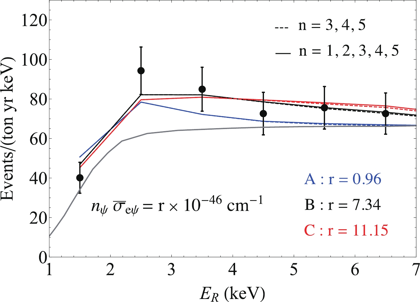
Figure A1. (color online) Contributions from K-shell and L-shell electrons in Xenon for the benchmark model points. The solid (dashed) lines include (exclude) the n = 1,2 electrons in Xenon.
On-shell mediator dark matter models and the Xenon1T excess
- Received Date: 2020-08-06
- Available Online: 2021-01-15
Abstract: We present a dark matter model to explain the excess events in the electron recoil data recently reported by the Xenon1T experiment. In our model, dark matter


 DownLoad: