


 Abstract
 HTML
HTML Reference
 Related
 PDF
PDF


-
Although the Standard Model (SM) in particle physics has achieved great success in phenomenology, there still exist many problems (such as the dark matter puzzle, hierarchy issue, and flavor problem) that the SM does not address, leading researchers to believe in the existence of physics beyond the SM (BSM). Popular BSM scenarios include supersymmetry (SUSY), in particular the minimal supersymmetric Standard Model (MSSM) (sometimes with different prefixes, such as NMSSM, PMSSM, and CMSSM [1-5], that extend the MSSM with additional fields) and composite/little Higgs models with TeV-scale strong dynamics [6-9].
As one of the most fully fledged scenarios of BSM physics, SUSY has good motivations from both the theoretical and phenomenological points of view. In semi-realistic string theories, which are probably among the most competent fundamental quantum theories that incorporate gravity, supersymmetries are required for deep reasons. Supersymmetries not only introduce fermionic degrees of freedom to the otherwise purely bosonic string theories but also elegantly ensure the stability of the system by eliminating the tachyons (states with negative mass squared that commonly appear in string theories). In contrast, phenomenologists particularly favor SUSY at low or intermediate scales. Such supersymmetric models provide a good mechanism to explain the large hierarchy between the electroweak (EW) scale and the Planck scale by canceling the quadratic divergence in the radiative corrections to the Higgs mass; they therefore save the Nature from being fine-tuned. Since experimental searches have ruled out a large portion of the parameter/model space for low-scale SUSY, researchers should now focus on supersymmetric models at or above the TeV scale.
In low- or intermediate-scale supersymmetric models, researchers usually work within the perturbative regime (except for the QCD part), likely in the interest of simplicity. In many UV-completed models, however, extra strongly coupled sectors are quite common. Ref. [10] shows how such strongly-interacting hidden sectors can arise in heterotic string theories. For discussions of strongly coupled sectors in the context of Type-II string theories, one may refer to Ref. [11], a follow-up phenomenological study of the intersecting D-brane models constructed in Refs. [12, 13]. A pedagogical review about intersecting D-branes, in particular about how the strongly coupled sectors appear, can be found in Ref. [14]. Non-perturbative effects are hard to calculate quantitatively. The study of the strongly coupled gauge theory and gauge/gravity duality has shed some light on non-perturbative calculations. The strongly coupled theory can be converted into a weakly coupled sector in the bulk, following the holographic principle. One example of SUSY breaking is as follows: the visible sector may talk to the strongly coupled hidden sector through messenger fields that are charged under both gauge sectors, as studied in the scheme of holographic gauge mediation [15].
In this study, we examine a class of BSM models with an extra strongly coupled hidden
$ SU(N)_H $ sector, along a similar line as in Refs. [16, 17]. We point out that this type of theory potentially alleviates the little hierarchy problem, and that it can be realized in a gauge-mediated SUSY breaking scenario. New scalars charged simultaneously under both the SM and hidden gauge groups are introduced for this purpose. We explore the possibility of achieving SM gauge coupling unification at an appropriate scale with the addition of these new particles. Such models appear much less fine-tuned in the Higgs mass without conflicts with direct search bounds at colliders. As a bonus, exotic bound states formed under the new strong dynamics appear as various diboson/dijet/diphoton resonances at different scales, the lightest of which may soon be discovered at colliders.We emphasize that, in our models, the new (supersymmetric) strong dynamics has entirely different signatures at colliders in comparison with scenarios such as low- or intermediate-scale perturbative SUSY, Goldstone Higgs [18, 19], and supersymmetric Goldstone Higgses [20]. The new scalars, despite being in the range of a few hundred GeV to TeV, can hadronize quickly into exotic mesons and baryons through the new strong dynamics. In contrast to the standard final state searches for squarks in SUSY, detecting the new scalars requires a different approach since they are confined in the bound states, and the new bound states decay more like pions and Goldstone particles, similar to the resonances in composite Higgs theories. Unlike in the composite-Higgs/technicolor scenarios, Higgs bosons are fundamental particles in our scenarios. Therefore, our models are free from many electroweak precision constraints.
The paper is organized as follows. In Section II, we define the gauge groups of the models and provide the particle spectrum in both the non-supersymmetric and supersymmetric cases. The Higgs mass fine-tuning issue is studied in Section III. In Section IV, we explore the conditions on the particle content of our models needed for the SM gauge coupling unification to be achieved at an appropriate scale. In Section V, we discuss existing experimental constraints on the new scalar masses and list possible exotic bound states formed from the new degrees of freedom as well as possible dark matter candidates. In Section VI, we discuss the collider phenomenology of the new mesons arising from our models, discussing in some detail their diphoton/diboson/dijet signatures at the LHC. Concluding remarks are given in Section VII.
-
We extend the SM by adding complex scalar multiplets charged as fundamentals under a hidden
$ SU(N)_H $ gauge group with a confinement scale of$ \Lambda_H\sim{\cal O}(1) $ TeV. All the SM fields are neutral under the hidden gauge group. We choose the SM charges of the new particles as given in Table 1, so that one generation of them and their conjugates can be neatly embedded into partial or full irreducible representations of an$ SU(5)_V $ gauge group, which potentially unifies the SM gauge groups$ SU(3)_C\times SU(2)_L\times U(1)_Y $ , where the subscript V denotes the visible sector. We emphasize here that the new particles in the class of models we focus on are all listed in Table 1, but this does not imply that, for each model, the new particles must encompass the full spectrum presented in Table 1. In fact, each set of new particles defines a specific model. In order for the hidden gauge group$ SU(N)_H $ to be confined, the number of particles that are charged under the hidden group cannot be too large. We check this issue later in a specific model (26).${SU(N)_H}$ 

${SU(3)_C}$ 

${SU(2)_L}$ 

${U(1)_Y}$ 

${U(1)_{EM}}$ 

${\widetilde{Q}=(\widetilde{Q}_U,\,\widetilde{Q}_D)^T}$ 

${\bf{N}}$ 

3 2 ${1/6}$ 

${2/3,\,-1/3}$ 

${\widetilde{U'}^{\dagger}}$ 

${\bf{N}}$ 

${\overline{\bf{3}}}$ 

1 ${-2/3}$ 

${-2/3}$ 

${\widetilde{D}^{\dagger}}$ 

${\bf{N}}$ 

${\overline{\bf{3}}}$ 

1 ${1/3}$ 

${1/3}$ 

${\widetilde{L}=(\widetilde{L}_N,\,\widetilde{L}_E)^T}$ 

${\bf{N}}$ 

1 2 ${-1/2}$ 

${0,\,-1}$ 

${\widetilde{E}^{\dagger}}$ 

${\bf{N}}$ 

1 1 1 1 Table 1. Representations of some new messenger fields. The dagger denotes the Hermitian conjugate. The electric charge is related to the hypercharge through
${Q_{EM}=T_3+Y}$ .Explicitly, for the messenger fields, we have
$ \bar{{\bf{5}}} = \left(\begin{array}{c} \widetilde{D}^{\dagger}\\ \widetilde{L} \end{array}\right), $

(1) $ {\bf{10}} = \left({\begin{array}{*{20}{c}} 0 & \widetilde{U'}_{3}^{\dagger} & \widetilde{U'}_{2}^{\dagger} & \widetilde{Q}_{U1} & \widetilde{Q}_{D1}\\ -\widetilde{U'}_{3}^{\dagger} & 0 & \widetilde{U'}_{1}^{\dagger} & \widetilde{Q}_{U2} & \widetilde{Q}_{D2}\\ -\widetilde{U'}_{2}^{\dagger} & -\widetilde{U'}_{1}^{\dagger} & 0& \widetilde{Q}_{U3} & \widetilde{Q}_{D3}\\ -\widetilde{Q}_{U1} & -\widetilde{Q}_{U2} & -\widetilde{Q}_{U3} & 0 & \widetilde{E}^{\dagger}\\ -\widetilde{Q}_{D1} & -\widetilde{Q}_{D2} & -\widetilde{Q}_{D3} & -\widetilde{E}^{\dagger} & 0 \end{array}}\right), $

(2) where
$ \widetilde{D}^{\dagger} = \left(\begin{array}{c} \widetilde{D}^{\dagger}_{1}\\ \widetilde{D}^{\dagger}_{2}\\ \widetilde{D}^{\dagger}_{3}\end{array}\right),\quad \widetilde{L} = \left(\begin{array}{c} \widetilde{L}_N\\ \widetilde{L}_E\end{array}\right). $

(3) The wide tilde indicates that the new fields are scalars①. For convenience, we call the particles associated with the messenger fields hidden scalars. At this stage, we have not fixed the number of generations for each multiplet. In other words, in a specific model with a low energy effective theory, a multiplet may be present or absent, and the new multiplets may come in complete or incomplete
$ SU(5)_V $ 5/10-plets. As shown in Section IV, from the gauge coupling unification point of view, incomplete GUT representations are actually required.In addition to the new fields in Table 1, we consider a Higgs sector with two Higgs doublet fields, both neutral under
$ SU(N)_H $ , as shown in Table 2. Similar to the Two-Higgs Doublet Model (2HDM), one linear combination of the electrically neutral Higgs bosons is identified as the 125-GeV Higgs boson. There are a few distinct scenarios, depending on how the two Higgs fields couple with SM fermions. We emphasize here that, in our setup, the Higgs fields are fundamental, unlike in the usual technicolor or composite/little Higgs models in which the Higgses are (pseudo)-Goldstone bosons. Therefore, our models are exempt from the usual constraints of those models.${SU(N)_H}$ 

${SU(3)_C}$ 

${SU(2)_L}$ 

${U(1)_Y}$ 

${U(1)_{EM}}$ 

${H_u=( H^+_u,\, H^0_u)^T}$ 

1 1 2 ${1/2}$ 

${1,\,0}$ 

${ H_d=( H^0_d,\,H^-_d)^T}$ 

1 1 2 ${-1/2}$ 

${0,\,-1}$ 

Table 2. Representations of the Higgs doublets.
-
In this subsection, we briefly comment on the supersymmetric version of the above-mentioned setup. We assume that the hidden gauge fields are in the confined phase (this can be achieved for
$ 2\leqslant N $ , as we will show later). Since the hidden gauge field takes no SM charges, we focus on the messenger sector. The supersymmetric version of the setup discussed previously includes the MSSM in the visible sector, with chiral supermultiplets charged as presented in Table 1 (and their conjugates), and vector supermultiplets associated with the gauge fields in the hidden sector. We assume that all the MSSM gauginos and Higgsinos are either sufficiently heavy or completely decoupled from the SM so that bounds from the neutralino dark matter direct detection or the direct collider searches [21-24] can be avoided. In order to not introduce anomalies, we include vector-like fermions whose left-handed components are superpartners of the scalars in Table 1 and whose right-handed components take conjugate charges of those in Table 1. We denote the left-handed fermions as Q,$ U'^{\dagger} $ ,$ D^{\dagger} $ , L, and$ E^{\dagger} $ , and their superpartners are indicated with widetildes, as in Table 1. The corresponding right-handed fermions and their scalar superpartners are denoted by fields with bars, e.g.,$ \bar{Q} $ and$ \widetilde{\bar{Q}} $ ②.In order to allow a Yukawa coupling between the messenger fields and one Higgs doublet field in the superpotential, we introduce another left-handed chiral multiplet, which is embedded in another
$ SU(5)_V $ 10-plet and whose scalar component is charged as presented in Table 3.$ \widetilde{U}^{\dagger} $ is embedded in a 10-plet, which takes the same visible charges as$ \widetilde{U'}^{\dagger} $ ,$ \widetilde{Q} $ , and$ \widetilde{E}^{\dagger} $ but is antifundamental under the hidden gauge group$ SU(N)_H $ when compared to$ \widetilde{U}^{\dagger} $ .${SU(N)_H}$ 

${SU(3)_C}$ 

${SU(2)_L}$ 

${U(1)_Y}$ 

${U(1)_{EM}}$ 

${\widetilde{U}^{\dagger}}$ 

${\overline{\bf{N}}}$ 

${\overline{\bf{3}}}$ 

1 ${-2/3}$ 

${-2/3}$ 

Table 3. Representations of an additional new messenger field. The dagger denotes the Hermitian conjugate. The electric charge is related to the hypercharge through
$Q_{EM}=T_3+Y$ .The Yukawa-type superpotential takes the form
${W_{{\rm{mess2}}}} \supset {Y_U}\;{\Phi _{{{\widetilde U}^\dagger }}}{\Phi _{\widetilde Q}}{\Phi _{{H_u}}}\;,$

(4) where
$ \Phi_{\widetilde{Q}} $ ,$ \Phi_{\widetilde{U}^{\dagger}} $ , and$ \Phi _{H_u} $ refer to the left-handed (holomorphic) supermultiplets of the corresponding hidden scalars$ \widetilde{Q} $ ,$ \widetilde{U}^{\dagger} $ , and the Higgs$ H_u $ , respectively. The coupling of the right-handed superfields can be written in a similar manner. The hidden scalars$ \widetilde{U} $ and$ \widetilde{Q} $ thus exhibit interactions with$ H_u $ in the scalar potential$ V\supset -|Y_U|^2\left(H_u^{\dagger}H_u\widetilde{Q}^{\dagger}\widetilde{Q}+H_u^{\dagger}H_u\widetilde{U}^{\dagger}\widetilde{U}+\widetilde{Q}^{\dagger}\widetilde{Q}\,\widetilde{U}^{\dagger}\widetilde{U}\right) \; , $

(5) while the hidden fermions Q and U achieve a Yukawa coupling to
$ H_u $ in the Lagrangian$ {\cal L}_{\rm Yukawa}\supset -Y_U U^{\dagger}H_u Q + {\rm c.c.} \; . $

(6) Although our scenario does not depend greatly on the type of SUSY-breaking mediation, it is naturally a gauge mediation scenario with messenger fields. If we assume that SUSY in the hidden sector is spontaneously broken by a nonvanishing F-term vacuum expectation value (VEV)
$ \langle F \rangle $ , causing mass splitting between the fermion and scalar in any hidden chiral supermultiplet, the SUSY breaking effects are then transmitted to the visible sector via loops of the messenger particles where they modify the MSSM gaugino masses, while the masses of SM gauge bosons remain intact due to the gauge symmetries. The usual messenger superpotential in which a messenger multiplet$ \Phi_\phi $ couples to a singlet multiplet$ \Phi_S $ is$ W_{\rm mess1} = Y_S\Phi_S\Phi_\phi \bar{\Phi}, $

(7) with the F-term corresponding to
$ \Phi_S $ ,$ <F_S>\neq 0 $ . In addition to many gauge mediation models with$W_{\rm mess1}$ as above, there is another messenger superpotential (4). Therefore, messenger fermions and scalars receive contributions from both (4) and (7). In particular, the scalar potential includes$ V\ni \biggl|\frac{\partial (W_{\rm mess1}+W_{\rm mess2})}{\partial \phi}|^2+\biggl | \frac{\partial (W_{\rm mess1}+W_{\rm break})}{\partial S}|^2, $

(8) where both SUSY and SUSY-breaking contribution to the messenger scalar masses are considered. Generically, the messenger scalars in Table 1 are not in their mass eigenstates. For mass eigenstates with very large eigenvalues, they decouple from the low energy spectrum and may be identified as “those missing in the complete gauge unified multiplets,” as we will see in Chapter IV. Furthermore, (8) may not be the full scalar potential due to the existence of the hidden strong dynamics. The additional messenger superpotential (4) and hidden strong force make it possible that the messenger scalar masses are smaller than their fermionic superpartners, which is the opposite of the case in MSSM. Explicit derivation of the messenger mass eigenvalues requires knowledge of the complete messenger spectrum (which is to be determined in Chapter IV) and more details about the hidden sector. We leave this for the future work. In what follows, we assume that the messenger scalars are much lighter than the messenger fermions and use
$ M_{\rm{mess}} $ to denote a messenger scalar mass. Through SUSY-breaking mediation to the visible sector, the SM squarks obtain soft SUSY-breaking masses:$ m_{\rm{soft}} \sim \frac{\alpha}{4\pi} \frac{\langle F \rangle}{M_{\rm{mess}}} \; , $

(9) where
$ \alpha/4\pi $ is the loop factor for gauge mediation. The lightest messenger mass$ M_{\rm{mess}} $ in our set-up is relatively lower than that in the standard gauge mediation scenarios. Here,$ M_{\rm{mess}} $ can be a few hundred GeV. The vector-like hidden fermions are allowed to have SUSY-breaking mass terms:$ M_q (Q \bar{Q}+U^{\dagger}\bar U^{\dagger}+...) +{\rm c.c.}\; , $

(10) where we have denoted the messenger fermions schematically as
$ M_q $ . Both$ M_q $ and$ m_{\rm{soft}} $ are around the SUSY breaking scale of at least a few TeV, which implies$ \sqrt{\langle F\rangle } \gtrsim 10^4 $ GeV. -
The fine tuning of the Higgs potential in general comes from the quadratic dependence in quantum corrections involving two disparate energy scales (i.e., the weak scale and the grand unified or Planck scale). In our setup, the Higgs sector consists of two Higgs doublets, as shown in Table 2. The SM Higgs boson H with a mass of 125 GeV is a linear combination of the neutral components of these two doublets. A supersymmetric spectrum ensures that the quadratic divergence cancels within the superpartners, leaving SUSY-breaking logarithmic pieces.
The top Yukawa coupling
$ y_t $ in the SM fermion sector yields the dominant contributions to$ m^2_{H_u} $ at the one-loop level. The loop corrections to$ m^2_{H_u} $ can thus be used as a parameter to define “naturalness” [25, 26]. In our models, we can calculate the contribution from the SM sector and the strongly coupled hidden sector as follows, if we assume a high-scale supersymmetric spectrum. The contribution from the SM chiral multiplets reads$ \delta m^2_{H_u} \supset \frac{3g_2^2 }{8 \pi^2}\left(M_t^2\,{\rm{Ln}}\frac{\Lambda^2}{M_{t}^2}-M_{\widetilde{t}}^2\,{\rm{Ln}}\frac{\Lambda^2}{M_{\widetilde{t}}^2}\right), $

(11) where
$ M_t $ and$ M_{\widetilde{t}} $ denote the top and stop masses, respectively. We assume the SUSY breaking scale is much heavier than$ M_t,\, M_{\widetilde{t}} $ , and that it is around 30 TeV. Note that, here, we have not taken different SUSY-breaking schemes or RG running from the messenger scale to the stop scale into consideration. We simply take the dominant contribution from the mass splitting of the top quark and the top squark. We do not distinguish the flavor eigenstate and mass eigenstate either and simply assume that all masses here come from the mass eigenstates.Considering the contribution from the hidden sector, dominantly from the mass splitting between the hidden scalar and its associated fermion③, we have
$ \delta m^2_{H_u} \supset\frac{3Y_U^2 N_c }{4 \pi^2}\left(M_{Q}^2\, {\rm{Ln}}\frac{\Lambda^2+M_{Q}^2}{M_{Q}^2}-M_{\widetilde{Q}}^2\, {\rm{Ln}}\frac{\Lambda^2+M_{\widetilde{Q}}^2}{M_{\widetilde{Q}}^2}\right ), $

(12) where the extra factor of 2 comes from the vector-like generations; N is the hidden multiplicity due to the
$ SU(N)_H $ gauge group, and we have ignored a spectrum-dependent overall factor that results from transforming the messenger fields to their mass eigenstates.$ M_Q $ and$ M_{\widetilde{Q}} $ refer to the mass eigenvalue of the messenger fermion and that of the messenger scalar, respectively.With
$ M_{Q} \sim M_{\widetilde{t}} $ on the scale of a few TeV within the reach of next-generation colliders and$ M_{\widetilde{Q}} $ around scale of TeV being mainly in charge of canceling the quadratic divergence from the SM top quark, we define a naturalness parameter:$ \Delta^{-1} = \left| \frac{2\delta m^2_{H_u}}{m_H^2} \right| \; . $

(13) We plot a schematic mass spectrum of the top quark, the hidden scalar, and their superpartners in Fig. 1. The contour of
$ \Delta $ on the$ M_{\widetilde{Q}} $ -$ M_{Q} $ plane is shown in the left panel of Fig. 2. In the right panel, we assume a very high-scale SUSY spectrum by setting the stop and hidden fermion masses to infinity. Here we have only considered the quadratic divergence coming from the top related sector at the one-loop level and set N to 2 in both plots, as suggested in Section IV. The quadratic contributions to the Higgs mass coming from the other SM particles are much smaller and can presumably be canceled by introducing corresponding new particles at higher energies. It is noted that, with higher multiplicities, the fine-tuning problem becomes worse. Moreover, perfect cancellation requires an ad hoc relation between$ y_t $ and$ Y_U $ .
Figure 1. A schematic mass spectrum of the top quark, the hidden scalars, and their superpartners. The lightest hidden scalar mass is assumed to be around 300 GeV or above to evade the electroweak precision and Higgs data bounds, while the lightest mesonic bound states are around the TeV scale. The MSSM stop
$\widetilde{t}$ and fermions from the hidden sector multiplets Q are of at least a few TeV.
Figure 2. (color online) Left panel: contours of the fine-tuning parameter
$\Delta$ in the hidden scalar mass and associated hidden fermion mass plane, with the mass of the MSSM stop being fixed at 3 TeV, and$\Lambda \sim 50$ TeV.$\Delta$ diverges as the logarithmic part of one-loop corrections to the Higgs mass completely cancels in the white region. Right panel:$\Delta$ as a function of the hidden scalar mass in the very-high scale SUSY case, in which the contributions of the MSSM stop$\widetilde{t}$ and hidden fermion Q are not considered. We set$N=2$ in both plots, as suggested in Section IV. -
It is tempting to see whether the new particles together with the SM particles (and possibly some other particles) can be embedded into a larger gauge group
$ SU(5)_{V}\times SU(N)_H $ . Researchers have studied the Grand Unified Theories (GUT) and their applications in phenomenology extensively [27-37]. In this section, we explore the conditions under which the SM gauge couplings can be unified at a GUT scale$ M_{\rm GUT} $ . For simplicity, we assume that there is no intermediate stage of the symmetry breaking$ SU(5)_V\to SU(3)_C\times SU(2)_L\times U(1)_Y $ , and that the visible group is spontaneously broken down to the SM gauge group due to “GUT-Higgs” scalars in the adjoint representation 24 acquiring a nonvanishing VEV as usual:$ \langle {\bf{24}} \rangle = {\rm{diag}}\left(2,\,2,\,2,\,-3,\,-3\right) v \; . $

(14) At the one-loop level, we want the SM gauge couplings
$ \alpha_a = g_a^2 /(4\pi) $ ④ to be unified at an appropriate GUT scale:$ \alpha_3(M_{\rm GUT}) = \alpha_2(M_{\rm GUT}) = \alpha_1(M_{\rm GUT})\equiv\alpha_{\rm GUT} \; , $

(15) with the following additional conditions:
1. The couplings remain within the perturbative regime at the GUT scale, i.e.,
$ 0 < \alpha_{\rm GUT} < 1. $

(16) 2. The GUT scale stays within an appropriate range. We require the GUT scale to be lower than the fundamental string scale
$ M_s $ (which is lower than the reduced Planck mass$ M_P $ ). On the other hand, the GUT scale should be high enough not to incur a fast proton decay. Since the quarks and leptons are in the same GUT representation, protons can decay via higher dimensional baryon number violating operators. Dimensional analysis indicates the proton lifetime as$ \tau _p\sim M^4_{X}/m_p^5 $ , where$ m_p $ is the proton mass, and$ M_X\sim M_{\rm GUT} $ is the mass of the GUT gauge bosons that acquire mass when the GUT group is broken. A detailed calculation [38, 39] shows that the experimental Super-Kamiokande limit [40]$ \tau_p>5.3\times 10^{33}\,{\rm{yr}} $ requires$ M_{\rm GUT} > 6\times 10^{15}\,{\rm{GeV}} \times \left(\frac{\alpha_{\rm GUT}}{1/35}\right)^{1/2}\left(\frac{\alpha _N}{0.015\,{\rm{GeV}}}\right)^{1/2}\left(\frac{A_L}{5}\right)^{1/2} \; , $

(17) where the operator renormalization factor
$ A_L $ and the hadronic matrix element$ \alpha_N $ are 5 and 0.015 GeV, respectively, from a lattice calculation [41].The unification condition (15) leads to
$ \alpha_{\rm GUT}^{-1} = \alpha_3^{-1}(M_Z) + \frac{b_3}{4\pi}{\rm{ln}}\left(\frac{M_Z}{M_{\rm GUT}}\right)^2, $

(18) $ \alpha_{\rm GUT}^{-1} = \alpha_{EM}^{-1}(M_Z){\rm{sin}}^2\theta_W(M_Z) + \frac{b_2}{4\pi}{\rm{ln}}\left(\frac{M_Z}{M_{\rm GUT}}\right)^2, $

(19) $ \alpha_{\rm GUT}^{-1} = \frac{3}{5}\alpha_{EM}^{-1}(M_Z){\rm{cos}}^2\theta_W(M_Z) + \frac{b_1}{4\pi}{\rm{ln}}\left(\frac{M_Z}{M_{\rm GUT}}\right)^2, $

(20) where
$ b_a\,(a = 1,\,2,\,3) $ are the one-loop beta functions determined by the particle contents running in the loop (see Appendix (A2) for more details), and we have taken into account$ e = g_2{\rm{sin}}\theta_W = g_Y{\rm{cos}}\theta_W = \sqrt{\frac{3}{5}}g_1{\rm{cos}}\theta_W = \sqrt{4\pi\alpha_{EM}}. $

(21) We allow the error on the coupling unification to be no more than 5%:
$ |\alpha_i^{-1}-\alpha _1^{-1}| / \alpha_1^{-1} \leqslant 5 $ % for$ i = 2 $ and 3, and we take the central values of the following measured quantities [42]:$ \begin{aligned}[b] M_Z =& (91.1880\pm 0.0020) {\rm{GeV}} \; , \\ \alpha_3(M_Z) =& 0.1193\pm 0.0016 \; , \\ \alpha_{EM}^{-1}(M_Z) = & 127.916\pm 0.015 \; , \\ \sin^2\theta_W = & 0.22333\pm 0.00011 \; . \end{aligned} $

(22) Under the unification conditions (15), (16), and (17) and considering the fact that
$ b_i $ should not be smaller than the SM values, i.e.,$ b_1\geqslant \dfrac{41}{10},\,b_2\geqslant -\dfrac{19}{6},\,b_3\geqslant -7 $ , we can find constraints on the$ b_i $ values.In the following, we constrain the new matter fields in Table 1 and Table 3 as necessary for the gauge coupling unification, and we assume that they have different numbers of generations
$ n_a $ , where$ a = Q,\,U,\,D,\,L,\,E,\,U' $ . -
The supersymmetric spectrum of our models consists of the MSSM particles in the visible sector, new scalars and their vector-like superpartners charged under both the visible and hidden groups, and the hidden vector supermultiplets. In the traditional SUSY
$ SU(5) $ GUT models [43, 44], SM gauge coupling unification is attained at$ M_{\rm{GUT}} = (2 - 3) \times 10^{16}\,{\rm{GeV}} $ , with the beta functions$ (b_1,\,b_2,\,b_3)_{\rm MSSM} = \left(\frac{33}{5},\,1,\,-3\right), $

(23) where the masses of all the superpartners of the SM particles have been set at 1 TeV for simplicity. These masses can vary slightly, from a few hundred GeV to a few TeV, and do not greatly affect the result.
First, let us consider adding complete GUT multiplets to the spectrum. Suppose that we add
$ n_5 $ generations of$ \bar{{\bf{5}}} $ ,$ n_{10} $ generations of 10, and$ n_{10'} $ generations of$ {\bf{10'}} $ , where$ \bar{{\bf{5}}} $ and$ {\bf{10'}} $ are the extra particles given by Eqs. (1) and (2), respectively, and 10 is the 10-plet that incorporates the multiplet$ \widetilde{U}^{\dagger} $ charged as in Table 3. We assume that the SUSY breaking scale is 5 TeV. Above 5 TeV, the beta functions are⑤$\begin{aligned}[b] & {b_1} = \frac{{33}}{5} + N({n_5} + 3{n_{10}} + 3{n_{10'}})\;,\\ & {b_2} = 1 + N({n_5} + 3{n_{10}} + 3{n_{10'}})\;,\\ & {b_3} = - 3 + N({n_5} + 3{n_{10}} + 3{n_{10'}})\;, \end{aligned}$

(24) where the factor of N in the second terms comes from the fact that all the particles in Table 1 are fundamental under the hidden group. The lower indices 10 and
$ 10' $ refer to the 10-plets involving$ \widetilde{U}^{\dagger} $ and$ \widetilde{U'}^{\dagger} $ , respectively. As discussed earlier, we need the existence of multiplets$ \Phi_{\widetilde Q} $ and$ \Phi_{\widetilde U^{\dagger}} $ in order to have a Yukawa coupling to the Higgs in the superpotential, implying both$ n_{10},\,n_{10'}\geq 1 $ . We find that adding at least 1 generation of these two 10-plets to the otherwise (approximated) unified MSSM spectrum ruins the gauge coupling unification due to the Landau pole. Even if we instead add incomplete GUT representations, the minimal requirement of at least one$ \Phi_{\widetilde Q} $ and one$ \Phi_{\widetilde U^{\dagger}} $ still blows up the running couplings at high energies. This reflects the fact that we have added too many particles to the low-energy (compared to the GUT scale) spectrum. It also indicates that our models favor a split-SUSY scenario, in which some of the SM superpartners and the new fermions are at the GUT scale. Note that how the spectrum splits is model-dependent and that it differs from that in the standard split-SUSY scenarios in which Higgsinos and gauginos are the lightest superpartners.For simplicity and to avoid adding too many new particles due to their hidden multiplicities N, in what follows, we restrict our models to the
$ N = 2 $ case, though analysis shows that$ N = 3 $ also works for achieving the SM gauge coupling unification. -
In this subsection, we consider the unification conditions when only the new scalar parts of the multiplets charged under
$ SU(2)_H $ exist at low energies. This may be viewed as a decoupling limit of the non-traditional split-SUSY scenario (mentioned at the end of the last subsection), in which all the superpartners are at the GUT scale. We focus on the scenario in which the new scalar masses are below the confinement scale$ \Lambda_H $ and only new scalars in Table 1 are taken into account. Hereafter, we drop the prime notation in$ \widetilde{U'}^{\dagger} $ since for the$ SU(2)_H $ case, the multiplet$ \widetilde{U'}^{\dagger} $ identifies with the one without a prime,$ \widetilde{U}^{\dagger} $ . For definiteness, we assume in this subsection that$ \Lambda_H = 4\,{\rm{TeV}} $ , the masses of the extra Higgs bosons and all the new scalars are about 300 GeV, and those new scalars form bound states with masses of around 800 GeV or higher. We find the beta functions above the confinement scale$ \Lambda_H $ to be$ \begin{aligned}[b] b_1 = & \frac{41}{10} +\frac{1}{20}+\frac{1}{5}\left(\frac{n_Q}{6}+\frac{4n_U}{3}+\frac{n_D}{3}+\frac{n_L}{2}+n_E\right) \; , \\ b_2 = & -\frac{19}{6}+\frac{1}{6}+\frac{n_Q}{2}+\frac{n_L}{6} \; , \\ b_3 = & -7+\frac{n_Q}{3}+\frac{n_U+n_D}{6} \; , \end{aligned} $

(25) where the first term in each
$ b_a $ is purely the SM contribution, and the second terms in$ b_1 $ and$ b_2 $ come from the contributions of the additional Higgs degrees of freedom.We focus on one type of solution that achieves the gauge coupling unification:
$ \begin{aligned}[b] & n_Q = n_U = 2 \; ,\,n_D = n_L = 3 \; ,\,n_E = 0 \; ,\quad {\rm{or}} \\ & n_Q = n_U = 3 \; ,\,n_D = n_L = n_E = 0 \; , \end{aligned} $

(26) with the unification scale
$M_{\rm GUT}\sim8.87\times 10^{15}$ GeV, as shown in Fig. 3. One can easily check that the one-loop beta function for$ SU(2)_H $ is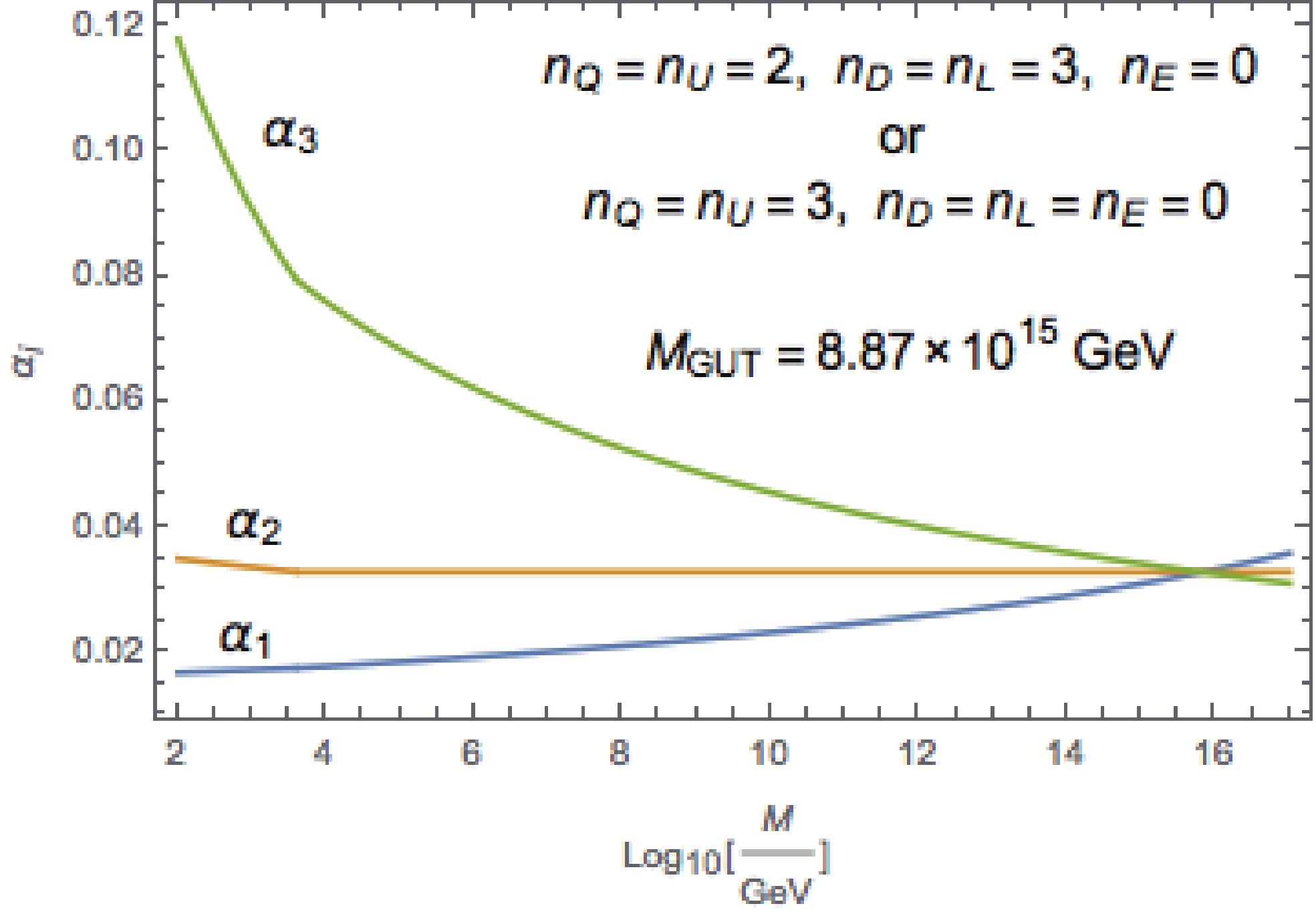
Figure 3. (color online) Running gauge couplings of a non-supersymmetric scenario. The new scalars and the extra Higgs bosons are taken to have a mass of 300 GeV. Below the confinement scale
$\Lambda_H=4\,{\rm{TeV}}$ , all the new scalars form bound states.$ b_{H2} = -\frac{11}{3}\times 2+\frac{1}{6}\times 2\times \frac{1}{2}\times (3\times 3\times 2+3\times 3) = -\frac{22}{3}+4.5<0, $

(27) if there is no purely hidden matter field. Therefore, as lo-ng as too many purely hidden degrees of freedom are not there, the
$ SU(2)_H $ may be asymptotically free in the UV.Below
$ \Lambda_H $ , all the new scalars presumably form mesons (as listed in Table 5). Therefore, they do not contribute to the beta functions. One can verify that even if a baryon with nontrivial$ SU(2)_L $ and$ U(1)_Y $ charges (see Table 6) is formed below$ \Lambda_H $ , its contributions to the running couplings are negligible due to the small value of$ \Delta b_i\times {\rm{ln}}\,\dfrac{4\,{\rm{TeV}}}{800\,{\rm{GeV}}} $ ⑥. The threshold corrections induced by non-perturbative effects around the hidden confinement scale are neglected.In the example of Eq. (26), the new scalars in the spectrum form incomplete GUT representations. The existence of incomplete GUT representations at low energies is typical in four-dimensional (4D) GUT theories. One famous example is the Higgs doublet-triplet splitting problem, namely in the splitting
$ {\bf{5}} \to \left( {\bf{3}},\,{\bf{1}},\,-\frac{1}{3} \right) + \left( {\bf{1}},\,{\bf{2}},\,\frac{1}{2} \right) \; , $

(28) $ \bar{{\bf{5}}}\to \left( \bar{{\bf{3}}},\,{\bf{1}},\,\frac{1}{3} \right) + \left( {\bf{1}},\,{\bf{2}},\,-\frac{1}{2} \right) \; . $

(29) The colored triplets are heavy, while the
$ SU(2)_L $ doublets are light. This splitting may be related to the$ \mu $ problem. The doublets and the triplets attain masses via a superpotential with coupling to an adjoint field and a$ \mu $ term upon the GUT symmetry breaking:$ \begin{aligned}[b] W_5 & = \lambda \,\bar{{\bf{5}}}\cdot {\bf{24}}\cdot {\bf{5}}+\mu \,\bar{{\bf{5}}}\cdot{\bf{5}}\\ &\Rightarrow\left(2\lambda v+\mu\right)\bar{{\bf{3}}}\cdot{\bf{3}} + \left(-3\lambda v+\mu\right)\bar{{\bf{2}}}\cdot{\bf{2}} \; . \end{aligned} $

(30) With v around the GUT scale and doublets at
$ {\cal O}(100) $ GeV, tuning of the$ \mu $ parameter is needed. In the case of$ SO(10) $ GUT, one way to explain the doublet-triplet splitting is via the Dimopoulos-Wilczek mechanism [29]. Generally, the strategy of generating such mass splitting in a GUT multiplet is to construct a superpotential in such a way that some components of the multiplet get masses around the GUT scale and thus decouple from the low-energy spectrum. However, this requires a careful arrangement of the VEVs of the other fields (in particular, singlets) in the superpotential and is usually complicated.The mass splitting issue may also be explored in the context of extra spacial dimensions withorbifold (For a pedagogical review, see for instance Ref. [45].). The idea is that fields localized at the fixed points of the internal space survive the orbifold actions and remain as complete multiplets in 4D, while fields living in the bulk are partially projected out and thus form incomplete multiplets (Such a scenario commonly appears in local GUT models in which the SM gauge symmetry arisesas intersections of several larger symmetries at different orbifold fixed points [46].). Whether a GUT multiplet lives in the bulk or at a fixed point is model-dependent. The masses that the bulk fields acquire are not arbitrary, even in the case of extra scalars and vector-like fermions. They must be induced by the VEVs of some auxiliary singlets (In string models, these massive bulkfields must satisfy the string selection rules [47].).
We assume that there exists an underlying higher dimensional theory that generates the mass splitting in the example of Eq. (26) and leave the explicit construction of an orbifold model giving such a spectrum to a future work.
-
As alluded to earlier, we have assumed that the hidden strong dynamics with an
$ {\cal O} (1) $ -TeV confinement scale has a much shorter hadronization time scale than QCD to ensure that the new scalars form bound states before they decay. The conventional collider constraints on the R-hadrons may not completely apply to our models since in addition to QCD, the hidden force plays a more dominant role in bound state formation. Direct searches of the hidden scalars are also very different from those of squarks/sleptons in the MSSM. However, we still have some indirect bounds coming from the electroweak precision constraints of LEP experiments since most of our new particles have SM charges and may couple to the SM Higgs boson. The bounds on the electroweak S, T, W, Y parameters due to the hidden scalars are similar to the supersymmetry precision bounds given in Ref. [48]. New hidden scalars that are heavier than a couple hundred GeV are safe from the constraints. These bounds can be further relaxed by decoupling the hidden scalars from the SM Higgs boson, which does not greatly change the phenomenology of our bound states.Another indirect bound comes from the Higgs data since the hidden scalars running in the loops modify the Higgs production and branching ratios, mostly constrained from the
$ H \rightarrow \gamma\gamma $ and$ H\rightarrow gg $ channels (see Fig. 4). Again, hidden scalars heavier than 300 GeV are safe [49]. Although in our models, the hidden scalars come from the hidden chiral multiplets as extensions to the MSSM, the indirect bounds still apply.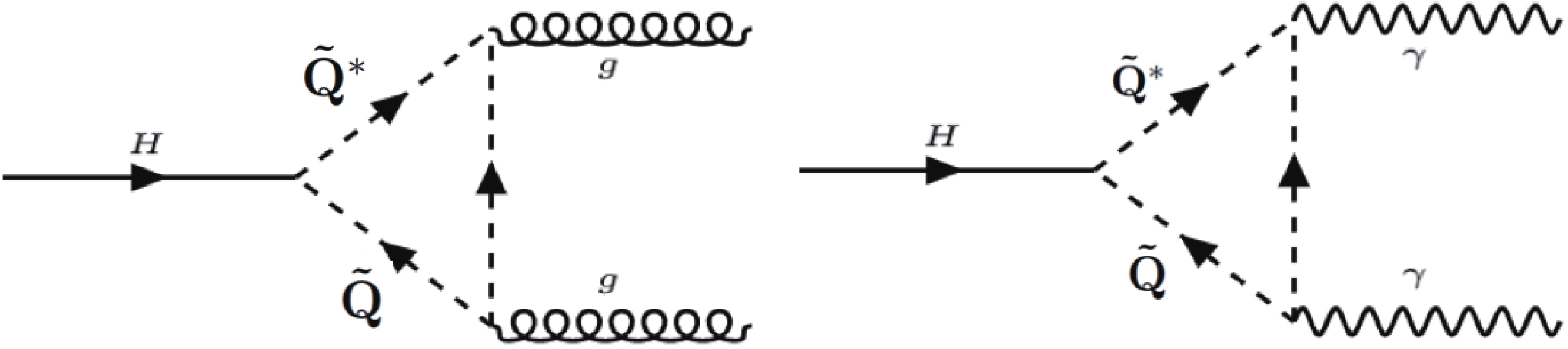
Figure 4. The scalar quarks from the hidden sector can modify the Higgs production rate and branching ratios through the loops.
-
The hidden scalars (possibly with the SM particles) form exotic bound states under
$ SU(2)_H $ . For now, we only focus on the lightest bound states with 2 matter particles and assume that all the vector-like fermions, if they exist, have a mass of at least a few TeV⑩.To determine all the possible bound states, in Table 4, we list relevant products of irreducible representations under different gauge groups that contain singlets under SM and hidden strong interactions.
${SU(2)}$ 

${\bf{2}\otimes \bf{2}}$ 

${SU(3)}$ 

${\bf{3}\otimes \bar{\bf{3}}}$ ,

${\bf{3}\otimes \bf{3}\otimes \bf{3}}$ 

Table 4. Products of irreducible representations that contain singlets. The conjugate representations are not listed.
-
The exotic mesons are of the type
$ A A^{\dagger} $ , listed in Table 5, where A refers to an exotic particle from Table 1, and the dagger indicates its conjugate. They are neutral under both visible and hidden gauge groups.Exotic Mesons ${\widetilde{Q}\widetilde{Q}^{\dagger}}$ ,

${\widetilde{U}\widetilde{U}^{\dagger}}$ ,

${\widetilde{D}\widetilde{D}^{\dagger}}$ ,

${\widetilde{L}\widetilde{L}^{\dagger}}$ ,

${\widetilde{E}\widetilde{E}^{\dagger}}$ 

Table 5. Exotic mesons formed from hidden scalars that are neutral under both SM and hidden gauge groups.
We assume that the masses of the lightest hidden scalars do not exceed the hidden confinement scale
$ \Lambda_H $ . Compared to the SM mesons, among which the lightest is CP-odd, the lightest composite state in our models is instead expected to be a CP-even neutral meson, as the result of an S-wave bound state of the messenger scalars.The supersymmetric setup can be compared to models with fermionic bi-fundamental constituents (e.g., composite/little Higgs models), where the lightest singlet appears as a Goldstone boson mode. In those models, one of the neutral Goldstone bosons becomes heavier than the SM-charged Goldstone bosons due to the chiral anomaly of the hidden gauge interaction. The neutral composite states in our scenario can be lighter due to mixing among the exotic mesons and possibly due to the hidden glueball, which can couple to the SM gauge bosons through scalar-loop diagrams (see also Ref. [50]).
-
Under
$ SU(2)_H $ , the exotic baryons that consist of 2 matter particles have the form$ AA' $ , where A and$ A' $ denote distinct hidden scalars (or their conjugates), i.e.,$ A' \neq A^{\dagger} $ . They are listed in Table 6.${AA'}$ 

${SU(2)_L}$ 

${U(1)_Y}$ 

${U(1)_{EM}}$ 

${\widetilde{Q}\widetilde{U}^{\dagger}}$ 

${\bf{2}}$ 

${-\dfrac{1}{2} }$ 

${-1,\,0}$ 

${\widetilde{Q}\widetilde{D}^{\dagger}}$ 

${\bf{2}}$ 

${\dfrac{1}{2} }$ 

${0,\,1}$ 

${\widetilde{L}\widetilde{E}^{\dagger}}$ 

${\bf{2}}$ 

${\dfrac{1}{2} }$ 

${0,\,1}$ 

${\widetilde{L}\widetilde{E}}$ 

${\bf{2}}$ 

${-\dfrac{3}{2} }$ 

${-2,\,-1}$ 

${\widetilde{U}\widetilde{D}^{\dagger}}$ 

${\bf{1}}$ 

${1}$ 

${1}$ 

Table 6. Exotic baryons as
${SU(2)_L}$ doublets and singlets and their Abelian charges. The conjugate particles are not listed.We note that unlike in the QCD and composite-Higgs models, the baryon masses in our models are not correlated with the confinement scale
$ \Lambda_H $ . This is because the baryons in our models are constructed by complex scalars instead of (approximate) chiral fermions.We briefly mention the existence of the
$ AA'a $ type of exotic baryon states, where A and$ A' $ are new hidden scalars (or their conjugates), and a refers to an SM quark. One example is the bound state$ \widetilde{Q}\widetilde{Q}u_R $ , which is a singlet or triplet under$ SU(2)_L $ , taking hypercharge 1 and electric charge 0,$ \pm 1 $ , or$ \pm 2 $ . For these bound states,$ AA' $ forms an$ SU(2)_H $ singlet with a nontrivial QCD charge and then forms a bound state with an SM quark by the QCD strong force. Since the QCD confinement scale$\Lambda_{\rm QCD}\sim {\cal O} (100)$ MeV is much lower than the hidden confinement scale$ \Lambda_H\sim {\cal O} (1) $ TeV, we expect the$ AA'a $ bound states to be much more unstable than the$ AA' $ baryons. Since the$ AA'a $ -type baryons have various$ SU(2)_L $ charges (singlet, doublet, triplet, or quadruplet), their decay channels can be quite interesting (Their decays may require the existence of additionalparticles to mediate the interactions.). Bounds for long-lived R-hadrons formed from colored SUSY particles in exotic or split SUSY models may apply here [51-53]. Bound states that are$ {\cal O}(1) $ TeV in mass are generally safe from such constraints. We leave the analysis of their interactions and decay signatures at colliders to a future work. -
In this subsection, we explore the existence of a dark matter (DM) candidate among the exotic baryon states formed by the messenger fields. For the
$ SU(2)_H $ gauge group, the$ AA' $ -type baryons may or may not be stable, depending on whether there is a symmetry (or topology such that the exotic baryons can be interpreted as solitons) to ensure their stability. If such a symmetry exists, e.g., a hidden baryon number$ U(1)_H $ gives each particle in Table 1 a hidden baryon number 1/2, then the first three and the last baryons in Table 6 have hidden baryon number 1, while the fourth has hidden baryon number 0. Then, the lightest, electrically neutral one of the first three baryons can be a DM candidate, and the discussion of the corresponding relic abundance follows the line of Refs. [16, 17]. In that case, the DM baryons annihilate into a pair of lighter scalar non-baryonic composite states. The thermal relic abundance can be much lower than the observed DM density if the annihilation cross section (into mesons, glubeballs, etc.) saturates the unitarity bound [54]. As a rough estimate, the relic abundance of an$ AA' $ -type DM baryon is [16]$ \Omega _Bh^2\sim 10^{-5}\frac{1}{F(M_B)^4}\left(\frac{M_B}{1\,{\rm{TeV}}}\right)^2, $

(31) where
$ M_B $ is the mass of the DM baryon, denoted as B, and$ F(M_B) $ is the form factor of the interaction of the DM baryon with lighter states such that$ F = 1 $ when the unitarity limit is saturated. With the lightest new hidden scalar mass being$ \sim 300 $ GeV, we expect that the lightest exotic baryon and the lightest exotic meson should have roughly the same mass in the sub-TeV regime. As an example that will be discussed in the next section, we have$ \widetilde U $ and$ \widetilde Q $ significantly lighter than the other hidden scalars, with the former slightly lighter than the latter. In this case, the DM baryon would be slightly heavier than the lightest exotic meson. We note from (31) that as long as the form factor$ F(M_B) $ is not smaller than a certain value (i.e.,$ F(M_B)\gtrsim \left[\displaystyle\frac{10^{-5}}{0.12}\left(\displaystyle\frac{M_B}{1\,{\rm{TeV}}}\right)^2\right]^{1/4}\approx 0.096\left(\displaystyle\frac{M_B}{1\,{\rm{TeV}}}\right)^{1/2} $ for cold, non-baryonic DM), the DM baryon would not overclose the universe. A more exact calculation of the relic abundance requires detailed knowledge of the hidden strong dynamics, particularly the precise form of the form factor.The direct search for the DM candidate is through the couplings between the hidden scalars and the Higgs boson (The Z exchange for electrically neutral bound states may also contribute and face roughly the same constraints as estimated in Ref. [28].). In terms of the effective field theory (EFT) approach, this corresponds to the direct coupling between the DM baryon and the Higgs boson:
$ {\cal L}\ni \lambda _B B^{\dagger}BH^{\dagger}H, $

(32) where the coupling is of the same order as those of the couplings between the constituent new scalars and the Higgs boson. The corresponding DM elastic interaction with nuclei via the Higgs exchange leads to a spin-independent (SI) cross section [55]:
$ \sigma _{\rm SI} = \frac{\lambda_B^2}{4\pi m_h^4}\frac{m_N^4f_N^2}{M_B^2}\approx 1.36\times 10^{-44}{\rm{cm}}^2\times \lambda_B^2\left(\frac{1\,{\rm{TeV}}}{M_B}\right)^2, $

(33) where we have used the lattice result of the nucleon decay constant
$ f_N\approx 0.326 $ [56] in the SM, and$ m_N $ is the nucleon mass at around 1 GeV. An exact estimate depends on the DM mass and the coupling$ \lambda_B $ that encodes the effects of the hidden strong dynamics. It seems that this cross section can satisfy the current LUX limit [57]$ \sigma_{SI}\lesssim 1\times 10^{-44}{\rm{cm}}^2(M_B/1\,{\rm{TeV}}) $ and be within the reach of the proposed LUX-Zeplin (LZ) experiment [58] for a suitable value of$ \lambda_B $ . However, the interaction of a baryon with a nonvanishing hypercharge with nucleons through Z-boson can be dominant. In fact, the cross section of such a process reads [59]$ \sigma _{\rm SI}^{Z} = \frac{m_N^2M_B^2}{\pi (M_B+m_N)^2}\left(\frac{F_N}{\sqrt{2}}\right)^2, $

(34) where
$ F_N $ is an induced form factor with mass dimension −2:$ F_p = 2F_u+F_d\quad{\rm{for \; proton}},\quad F_n = F_u+2F_d\quad{\rm{for \; neutron}}, $

(35) with form factors
$ F_{u/d}\sim{\cal O}(1)/M_Z^2 $ . One finds that$ \sigma_{SI}^Z\sim{\cal O}(10^{-35})\,{\rm{cm}}^2 $ , which is much greater than the LUX limit. This shows that a DM candidate does not exist in the lowest exotic baryons formed by the messenger fields listed in Table 1 for the$ SU(2)_H $ gauge group. When one considers an$ SU(3)_H $ hidden gauge sector, instead of$ SU(2)_H $ , such dangerous Z-boson exchange interactions between a baryon and a nucleon can be turned off due to the existence of baryon states (consisting of 3 messenger scalars) that are neutral (which we call “completely neutral”) under both$ SU(2)_L $ and$ U(1)_Y $ (e.g.$ \widetilde{L}_N\widetilde{L}_E\widetilde{E}^{\dagger} $ ). The SI scatterings with nuclei for such baryons are dominated by the Higgs exchange, and their cross sections can thus satisfy the LUX limit and be within the reach of the LZ experiment. The lightest one of these completely neutral baryons can be a DM candidate.If there is no symmetry or topology to ensure the stability of the exotic baryons, they decay⑬. We leave the study of the decay patterns of the exotic baryons to a follow-up work.
-
The various bound states have rich phenomenology in colliders, with different masses and decay channels. Thus the most significant signatures of our models are a tower of resonances with different masses. Although any model with hidden strong dynamics or one in the context of GUTs can also predict such resonances, we emphasize that our models are quite different from the composite-Higgs/technicolor scenarios due to the existence of fundamental scalars and different types of fundamental degrees of freedom, as mentioned in Section I.
As the simplest and lightest bound states, here we focus on the phenomenology of the lightest exotic mesons at the LHC. We generically denote a scalar meson by S with mass
$ M_S $ and a pseudoscalar meson by P with mass$ M_P $ . One property distinguishing these two types of exotic mesons is that the latter cannot decay into a pair of Higgs bosons, while the former can, as long as the kinematics allows.As argued in the previous section, the lightest meson in our models has to be CP-even. We use an EFT approach to describe the dynamics of the bound states at low energies, similar to the formalism of pion interactions in strongly-coupled QCD. The detailed calculation is summarized in Appendix B. For definiteness and simplification, we make the following assumptions for the hidden scalar masses:
● Both
$ \widetilde Q $ and$ \widetilde U $ representations are degenerate, i.e.,$ m_{\widetilde Q_1} = m_{\widetilde Q_2} = ... \; ,\quad m_{\widetilde U_1} = m_{\widetilde U_2} = ... \; , $

(36) where the subscripts on
$ \widetilde Q $ and$ \widetilde U $ denote generations.● Both
$ \widetilde Q $ and$ \widetilde U $ have similar masses and are lighter than the other scalars, i.e.,$ m_{\widetilde{Q}}\approx m_{\widetilde{U}}<{\rm{ mass \; of \; other \; hidden \; scalars}} . $

(37) Under these assumptions, it is justifiable to consider glue-glue fusion (GGF) as the dominant production process for the exotic mesons⑭. Note that Eq. (37) follows one of the examples with the satisfactory gauge coupling unification given in Eq. (26).
As an explicit example, we consider a scalar resonance S of mass 2 TeV. Figure 5 shows the dependence of the branching ratios of S on
$ \cos\theta $ (left plot) and$ \Lambda_2/\Lambda_Y $ (right plot). The mixing angle$ \theta $ is defined in Eq. (B9) to denote the rotation angle when one converts the meson flavor eigenstates to the mass eigenstates. The suppression scales$ \Lambda_i $ ($ i = Y,\,2,\,3 $ ) encoding details of the hidden strong dynamics are defined in Eq. (B3). From Eq. (B11), one finds the relation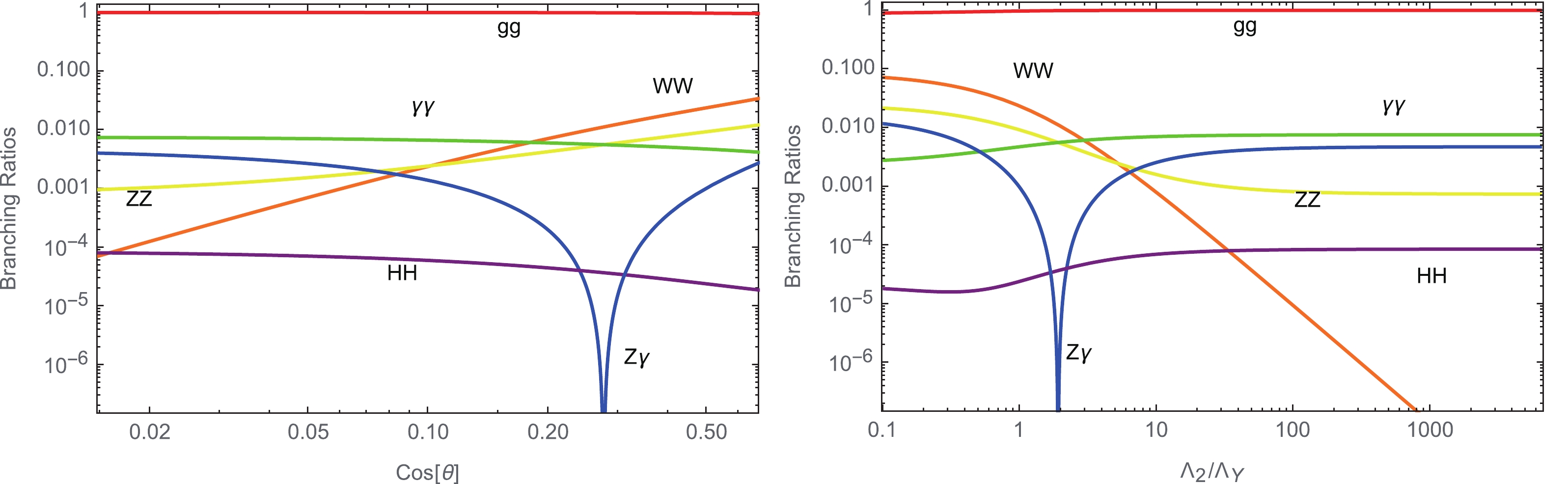
Figure 5. (color online) Branching ratios of the lightest scalar resonance of mass
$M_S = 2$ TeV decaying into the gauge boson pairs and the Higgs boson pair as functions of${\rm{cos}}\,\theta$ (left) and$\Lambda_2/\Lambda_Y$ (right) for$\Lambda_{H} = 4$ TeV. Both the left and right panels use$\lambda=0.01$ .$ 8|\tan\theta| = \biggl|\frac{15\Lambda_2}{\Lambda_Y}-1|. $

(38) In the numerical analysis given here, we use the running gauge coupling constants evaluated at the renormalization scale of
$ M_S $ , where new particles involved in the coupling running are taken as in Eq. (26). The cusps at$ {\rm{cos}}\,\theta\approx 0.27 $ and$ \Lambda_2/\Lambda_Y\approx 2 $ for the$ Z\gamma $ curves reflect the fact that the$ Z\gamma $ decay width vanishes if$ \dfrac{g_2^2}{\Lambda_2} = \dfrac{5}{3}\dfrac{g_Y^2}{\Lambda_Y} $ , due to a destructive interference effect as seen in Eq. (B18). As S is purely composed of colored particles, the decay rate of S into gluons is preponderant, particularly when its effective coupling to the SM Higgs boson$ \lambda $ , defined in Eq. (B20), is diminishing. In these plots, we take$ \lambda = 0.01 $ . Therefore, the exotic mesons are dominantly produced via the GGF process. The branching ratio of the$ HH $ channel, proportional to$ \lambda^2 $ , is thus subdominant in most of the parameter space. For simplicity and definiteness, we neglect the effects of the operator in Eq. (B20) by assuming$ \lambda \to 0 $ , so that the di-Higgs bound [60] is trivially satisfied.With a small branching ratio, as shown in Fig. 5, it is expected that such a new scalar will probably first appear through the diphoton channel due to the clean signals at the LHC. Figure 6 shows the contours of the diphoton channel cross section at the 13-TeV LHC,
$ \sigma_{\gamma\gamma}^{(13\,{\rm TeV})} $ , on the$ \cos\theta $ -$ \Lambda_H $ plane (left plot) and the$ \Lambda_2/\Lambda_Y $ -$ \Lambda_H $ plane for a few representative values of$ \Gamma_S/M_S $ . Note that, here, we use$ M_S/2 $ as the factorization and renormalization scale when calculating the cross sections. The colored regions are excluded by the resonance searches using various decay channels in LHC Run-I and Run-II for$ M_S = 2 $ TeV: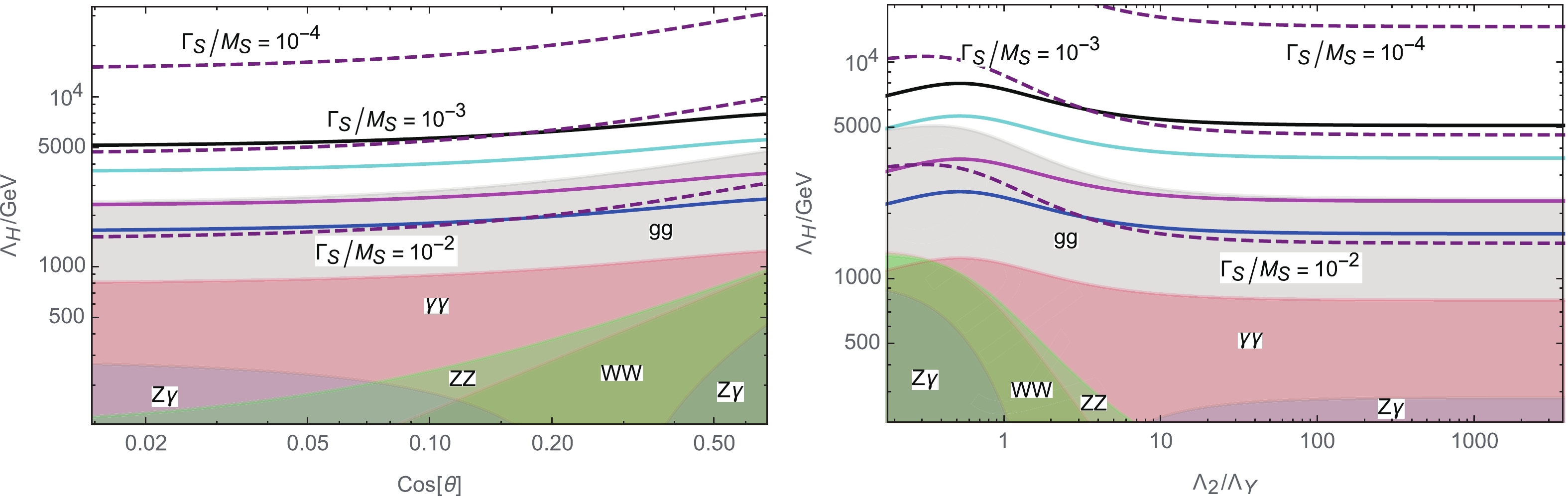
Figure 6. (color online) Contours of the production cross section of S times its decay branching ratio into
$\gamma\gamma$ at the 13-TeV LHC by assuming the glue-glue fusion production process. We fix$M_S = 2$ TeV and take the factorization and renormalization scales as$\mu = M_S/2$ . The dashed purple curves are contours for specific values of$\Gamma_S/M_S$ . The shaded regions are excluded by searches through various decay modes in LHC Run-I and Run-II, as detailed in Eq. (39). The black, cyan, magenta, and blue solid lines correspond to$ \sigma _{\gamma\gamma}^{(13\,{\rm TeV})} = 0.1,\,0.2,\,0.5,\,1$ fb, respectively.$ \begin{aligned}[b] & \sigma(pp\to S \to \gamma\gamma) < 0.3\,{\rm fb}\quad \rm[61, 62] \ ,\\ & \sigma(pp\to S \to WW) < 60\,{\rm fb}\quad \rm[63, 64, 71]\ , \\ & \sigma(pp\to S \to ZZ) < 8\,{\rm fb}\, \quad \rm[65, 70]\ , \\ & \sigma(pp\to S \to Z\gamma) < 20\, {\rm fb}\quad \rm[66, 72]\ , \\ & \sigma(pp\to S \to jj) < 70\,{\rm pb}\quad \rm[67-69, 73] \ . \end{aligned} $

(39) The figure shows that a certain parameter space predicts
$ \sigma_{\gamma\gamma}^{(13\,{\rm TeV})} = {\cal O}(0.1) $ fb, while avoiding all of the above constraints for an$ {\cal O}(1) $ TeV hidden confinement scale$ \Lambda_{H} \simeq 4\; {\rm TeV} \; , $

(40) with the relative suppression scale
$ \Lambda_2/\Lambda_Y \gtrsim 1 $ or$ {\rm{cos}}\,\theta \lesssim 0.5 $ . This result implies that$ \widetilde{U}^{\dagger} $ is slightly lighter than$ \widetilde{Q} $ in this specific example. Figure 6 (which reveals information about$ \Lambda_H $ , the messenger mass hierarchy, etc.) reflects the fact that the messenger resonances serve as a good probe of the new physics. Moreover,$\Gamma_S/M_S \sim $ $ {\cal O}(10^{-3}) $ , justifying the narrow width approximation employed in the numerical analyses.We now comment on the cross sections of the resonance decaying into other channels. Unlike the scenario in Ref. [16], for the specific example considered here, the branching ratios of the
$ WW $ ,$ ZZ $ ,$ Z\gamma $ modes change dramatically, as shown in Fig. 5. Instead of a simple, approximate proportionality relation between the cross sections of the other gauge boson modes and that of the diphoton mode, the ratios$ \sigma (pp\to S\to WW/ZZ/Z\gamma/ jj)\,/ \,\sigma(pp\to $ $S\to \gamma\gamma) $ depend on$ \cos\theta $ or$ \Lambda_2/\Lambda_Y $ in a more complicated way. Moreover, compared to Fig. 2 of Ref. [16], the contours of the di-photon cross sections in Fig. 6 vary less drastically as$ {\rm{cos}}\,\theta $ or the relative suppression scale$ \Lambda_2/\Lambda_Y $ changes. This is because in Ref. [16], the mixing is between one lepton-like scalar and one down-type quark-like scalar, whereas in our example, the resonance is made of only quark-like scalars. Such differences reflect the fact that the particle contents in the resonance meson greatly affect how the meson decays. When data on the other decay channels are available, we will know more about the nature of the particles involved in the lowest-lying resonance mesons. This may also shed light on the mass hierarchy in the hidden sector. Through such searches, the resonance structure may be revealed. -
We explore a class of models consisting of the Standard Model (SM) and a strongly coupled hidden
$ SU(N)_H $ sector. These models have various interesting phenomenological properties. First, by adding new messenger (hidden) fields taking special charges under the SM and the hidden gauge groups at low energies, the SM gauge couplings may unify at a suitable scale without inducing the fast proton decay issue. Their charge assignments are chosen so that they can be embedded into a larger gauge group$ SU(5)_V\times SU(N)_H $ . Analysis shows that a small-rank$ SU(N)_H $ ($ N = 2,\,3 $ ) gauge group and a split-SUSY scenario are favored. Second, the existence of new scalars provides an alternative solution to the electroweak hierarchy problem with or without SUSY. The Higgs mass can thus be less fine-tuned due to the cancellation between the top loop and the hidden scalar loop contributions. Third, in contrast to those in little-Higgs/composite-Higgs/technicolor models, the Higgs fields in our models are fundamental particles whose electroweak symmetry breaking pattern largely remains intact at low energy scales, indicating that our models suffer less from collider and electroweak precision observable constraints. Further studies of the properties of the new exotic resonances, such as the branching ratios to the SM particles, will distinguish our models from composite/little Higgs models. Finally, the models predict many exotic bound states formed under the hidden strong dynamics and the SM strong force. The bound states can cover a wide range of spectra, some of which will be within the reach of the LHC in the near future. They may also provide us with DM candidates with various weak charges and spins that have not yet been widely discussed in the literature. We leave the comprehensive study of the stability of the new bound states and their decay signatures to a future work.The potentially unified gauge theory and the strong hidden dynamics probably hint at the existence of an underling theory. In fact, our models may be smoothly implemented into string theory. The strongly coupled hidden
$ SU(N)_H $ sector can arise from the world volume gauge field living on a stack of D-branes and become part of the near throat strong warping AdS background geometry in the AdS/CFT limit, while the visible perturbative$ SU(5)_V $ sector can originate from another stack of D-branes that intersect with the hidden branes (and do not warp the throat). Open string modes at the intersections attaching to the two stacks of branes as bi-fundamentals under both$ SU(5)_V $ and$ SU(N)_H $ gauge groups play the role of messengers between the visible and hidden sectors. In this sense, our models may be viewed as a field theory realization of the so-called holographic gauge mediation [15], where the hidden$ SU(N)_H $ is studied in the large N limit as in holography.The year 1974 [74] was an exciting period for the community to first realize QCD as the gauge theory for strong interactions and to study the bound states of quarks. The LHC has opened a new era in particle physics. With QCD already established, it is tantalizing to speculate that there may be additional strongly coupled sectors in Nature. Such new strong dynamics may arise in different ways. They can be classified by whether they participate in the electroweak symmetry breaking and whether the new fundamental degrees of freedom are fermionic or bosonic. Through careful searches of their decay signatures in high-energy collisions, we may soon reveal the hidden strong dynamics at the LHC.
-
S.S. and F.Y. are grateful for the hospitality of NCTS, where this work was initiated. S.S. would like to thank Henry Tye, Ann Nelson, and Haipeng An for useful discussions about supersymmetry. F.Y. would like to thank Gary Shiu and Eibun Senaha for helpful discussions about gauge coupling unification.
-
At the one-loop level, the beta functions of the SM gauge coupling constants read
$ \alpha_a^{-1}(\mu) = \alpha^{-1}_a(\mu_0)+\frac{b_a}{4\pi}{\rm{ln}}\left(\frac{\mu_0^2}{\mu^2}\right), \tag{A1}$

where
$ a = 1,\,2,\,3 $ refer to gauge groups$ U(1)_Y $ ,$ SU(2)_L $ , and$ SU(3)_C $ , respectively. The group-theoretic coefficients$ b_a $ depend on the numbers of particles running in the loop:$ b_a = -\frac{11}{3}\sum_VC(R_V^a)+\frac{2}{3}\sum_{\rm Weyl}C(R_F^a)+\frac{1}{6}\sum_{\rm Real}C(R_S^a) \; , \tag{A2}$

where
$ R_V^a $ ,$ R_F^a $ , and$ R_S^a $ refer to the vector, Weyl fermion, and real scalar representations, respectively, under the gauge group labeled by a.$ C(R^a) $ values are the Dynkin indices defined through$ {\rm{Tr}}\left(T^A_RT^B_R\right) = C(R)\delta^{AB} \tag{A3}$

for the non-Abelian group representation R. We choose the normalization such that, for the fundamental representation
$ {\bf{N}} $ under$ SU(N) $ , the Dynkin index is$ C({\bf{N}}) = \frac{1}{2} \; . \tag{A4}$

Then, under
$ SU(N) $ , the Dynkin indices for the adjoint representation, the asymmetric tensor with rank 2, and the symmetric tensor with rank 2 are$ C(a) = N,\quad C(A_2) = \frac{N-2}{2},\quad C(S_2) = \frac{N+2}{2}, \tag{A5}$

respectively. Eq. (A2) can be applied to the Abelian group
$ U(1)_Y $ as well, by replacing$ C(R_V^a)\to 0 $ ,$ C(R_F^a)\to \displaystyle\frac{3}{5} Y_F^2 $ , and$ C(R_S^a)\to \displaystyle\frac{3}{5}Y_S^2 $ , where the$ Y_i $ values are hypercharges. The renormalization factor$ \displaystyle\frac{3}{5} $ is introduced as the hypercharge is identified with the diagonal generator of$ SU(5) $ , which does not belong to the Cartan subalgebras of$ SU(3) $ and$ SU(2) $ $ T^{24} = \sqrt{\frac{3}{5}} Y \; . \tag{A6}$

-
Effective interactions of a scalar S or a pseudoscalar P with the SM gauge bosons can be parametrized by
$ {\cal L}_{\rm eff} ^S = \frac{\kappa_3 ^{(S)}}{\Lambda_H}S G^a_{\mu\nu}G^{a\,\mu\nu} + \frac{\kappa_2^{(S)}}{\Lambda_H}S W^i_{\mu\nu}W^{i\,\mu\nu} + \frac{5}{3} \frac{\kappa_Y^{(S)} }{\Lambda_H}S B_{\mu\nu}B^{\mu\nu}\ , \tag{B1}$

$ {\cal L}_{\rm eff}^P = \frac{\kappa_3 ^{(P)}}{\Lambda_H}P \widetilde{G}^a_{\mu\nu}G^{a\,\mu\nu} + \frac{\kappa_2^{(P)}}{\Lambda_H}P \widetilde{W}^i_{\mu\nu}W^{i\,\mu\nu} + \frac{5}{3} \frac{\kappa_Y^{(P)}}{\Lambda_H}P \widetilde{B}_{\mu\nu}B^{\mu\nu}\ , \tag{B2}$

where
$ \Lambda_H $ is the emergent hidden strong dynamical scale. Here,$ G^{\mu\nu} $ ,$ W^{\mu\nu} $ , and$ B^{\mu\nu} $ denote the field strengths of the SM gauge bosons of the$ SU(3)_C $ ,$ SU(2)_L $ , and$ U(1)_Y $ groups, respectively, with the superscripts a and i being the indices for the corresponding adjoint representations. The coefficients$ \kappa_{3,2,1}^{(S/P)} $ are$ S/P $ -dependent$ {\cal O}(1) $ parameters and encapsulate details of the strong dynamics. One may define suppression scales for a canonically normalized$ S/P $ coupling to different gauge groups:$ \frac{1}{\Lambda_i} = \frac{\kappa_i^{(S/P)}}{\Lambda_H},\quad i = Y,\,2,\,3. \tag{B3}$

The kinetic terms of the gauge fields are
$ {\cal L} = - \frac{1}{4g_3^2} G^a_{\mu\nu}G^{a\,\mu\nu} - \frac{1}{4g_2^2} W^i_{\mu\nu}W^{i\,\mu\nu} -\frac{1}{4g_Y^{2}} B_{\mu\nu}B^{\mu\nu}\ , \tag{B4}$

where
$ g_3 $ ,$ g_3 $ , and$ g_Y $ are the corresponding gauge couplings.We assume any new complex scalar to be massive⑮:
$ {\cal L} \supset -m_{Qi}^2 \widetilde{Q}_i^\dagger \widetilde{Q}_i \; , \tag{B5}$

where
$ \widetilde{Q}_i $ here refers to any new particles in Table 1 with mass$ m_{Qi}\gtrsim 300 $ GeV, consistent with the current bounds from the electroweak precision observables and Higgs measurements, as discussed in Section VA. The mass can be even smaller if some of the new bi-fundamental scalars have suppressed couplings to the SM Higgs boson.The lightest meson made of the new scalars is kinetically normalized as
$ S = \frac{4\pi}{\kappa \Lambda_h}\sum _i O_{1i}[\widetilde{Q}^{\dagger}_i\widetilde{Q}_i] \; , \tag{B6}$

where the bracket refers to a meson state, and
$ 4\pi $ is introduced through Naive Dimensional Analysis (NDA) [75, 76]. The matrix$ O = (O_{ij}) $ is a special orthogonal matrix that brings the mesons to their mass eigenstates, and the scalar S corresponds to the first (lowest) eigenstate. The mesons in the original basis are$ [\widetilde{Q}_i^{\dagger}\widetilde{Q}_i] = \frac{\kappa\Lambda_H}{4\pi}\,O_{1i}\,S \; . \tag{B7}$

Plugging (B7) back into the effective Lagrangian with the mesons in the original basis, we can read off the suppression scales
$ \Lambda_1 $ ,$ \Lambda_2 $ , and$ \Lambda_3 $ as functions of$ O_{1i} $ values.In order to highlight the relation between the branching ratios of the lightest meson S and the mixings of particles forming S, let us assume that the flavors within the
$ \widetilde Q $ and$ \widetilde U $ multiplets are degenerate and that$ m_{\widetilde{Q}}\approx m_{\widetilde{U}}<{\rm{ mass \; of \; any\; other\; new \; scalars}} . \tag{B8}$

Note that Eq. (B8) may be viewed as a spacial case of the example shown in Eq. (26).
Under the above assumptions, the meson mass eigenstates S and T (with
$ M_S<M_T $ ) can be obtained through an$ SO(2) $ rotation parametrized by an angle$ \theta $ and a rescaling$ \left(\begin{array}{c} S\\ T\end{array}\right) = \frac{4\pi}{\kappa \Lambda_H}\left(\begin{array}{cc} {\rm{cos}}\,\theta & {\rm{sin}}\,\theta\\ -{\rm{sin}}\,\theta & {\rm{cos}}\,\theta\end{array}\right) \left(\begin{array}{c} \widetilde{Q}^{\dagger}\widetilde{Q}\\ \widetilde{U}^{\dagger}\widetilde{U}\end{array}\right), \tag{B9}$

where
$ \kappa \sim {\cal O}(1) $ . The effective Lagrangian of the mass eigenstates is$\begin{aligned}[b] {L_{\rm eff}}{ \ni } & \frac{\kappa }{{4\pi {\Lambda _H}}}\Bigg[ {(2{\rm{cos}} \theta + {\rm{sin}} \theta )S{G^2} + 3{\rm{cos}} \theta S{W^2} } \\ & \left. + {\left( {\frac{1}{3} {\rm{cos}} \theta + \frac{8}{3} {\rm{sin}} \theta } \right)S{B^2}} \right] + ...\;, \end{aligned} \tag{B10}$

where the ellipses refer to the couplings between the heavier meson T and gauge bosons. Thus, we can read the suppression scales
$ \begin{aligned}[b] & \frac{1}{\Lambda_3} = \frac{\kappa\bigl(2{\rm{cos}}\,\theta+{\rm{sin}}\,\theta\bigr)}{4\pi\Lambda_H} \; , \\ & \frac{1}{\Lambda_2} = \frac{3\kappa\,{\rm{cos}}\,\theta}{4\pi\Lambda_H} \; ,\\ & \frac{1}{\Lambda_Y} = \frac{3}{5}\frac{\kappa}{4\pi\Lambda_H} \left(\frac{1}{3}\,{\rm{cos}}\,\theta+\frac{8}{3}\,{\rm{sin}}\,\theta \right) \; . \end{aligned} \tag{B11}$

Through the effective couplings with the gluons and in the narrow width approximation, the scalar/pseudoscalar resonance is produced at the LHC via the gluon fusion process
$ \begin{aligned}[b] & \sigma(pp \to S/P) = \frac{\pi^2}{8} \left(\frac{\Gamma(S/P\to g+g)}{M_{S/P}}\right) \times \frac{1}{s}\frac{\partial{\cal L}_{gg}}{\partial\cal \tau} \; , \\ & \frac{\partial{\cal L}_{gg}}{\partial\cal \tau} = \int_0{\rm d}x_1 {\rm d}x_2 f_g(x_1) f_g(x_2) \delta (x_1 x_2 - \tau)\ , \end{aligned} \tag{B12}$

where
$ \tau = M_{S/P}^2/s $ and$ \sqrt{s} $ denote the center-of-mass energy of the proton-proton collisions. Using the MSTW PDFs [77], we obtain$ \frac{1}{s}\frac{\partial{\cal L}_{gg}}{\partial\cal \tau} \simeq \left\{\begin{array}{ll} 1.1\; {\rm pb} & ({\rm for } \sqrt{s} = 8\; {\rm TeV})\ ,\\ 15\; {\rm pb} & ({\rm for } \sqrt{s} = 13\; {\rm TeV})\ , \end{array}\right. \tag{B13}$

where we have fixed the factorization scale and the renormalization scale at
$ \mu = M_S/2 $ for$ M_S = 2 $ TeV.The partial decay widths of the scalar resonance are given by
$ \Gamma(S/P\to gg) = \frac{2}{\pi} \left( \frac{g_3^2}{\Lambda_3} \right)^2 M_{S/P}^3 \; , \tag{B14}$

$ \Gamma(S/P\to W^+ W^-) = \frac{1}{2\pi} \left( \frac{g_2^2}{\Lambda_2} \right)^2 M_{S/P}^3 \; , \tag{B15}$

$ \Gamma(S/P\to ZZ) = \frac{1}{4\pi} \left[ \left( \frac{g_2^2}{\Lambda_2}\right) c_W^2 + \frac{5}{3}\left( \frac{g_Y^{ 2}}{\Lambda_Y} \right)s_W^2 \right]^2 M_{S/P}^3 \; , \tag{B16}$

$ \Gamma(S/P\to \gamma\gamma) = \frac{1}{4} \frac{1}{\pi} \left[ \left( \frac{g_2^2}{\Lambda_2}\right) s_W^2 + \frac{5}{3}\left( \frac{g_Y^{ 2}}{\Lambda_Y} \right) c_W^2 \right]^2 M_{S/P}^3 \; , \tag{B17}$

$ \Gamma(S/P\to Z\gamma) = \frac{1}{2\pi} \left[ \left( \frac{g_2^2}{\Lambda_2}\right) - \frac{5}{3}\left( \frac{g_Y^{ 2}}{\Lambda_Y} \right) \right]^2 c_W^2s_W^2 M_{S/P}^3 \; , \tag{B18}$

where
$ s_W \equiv \sin\theta_W $ and$ c_W = (1-s_W^2)^{1/2} $ with$ \theta_W $ being the weak mixing angle. The masses of the W and Z bosons are neglected to a good approximation.The decay of S into a pair of the 125-GeV Higgs bosons is characterized by interactions between new particles and the Higgs boson H:
$ {\cal L} = \left(\lambda _Q\, \widetilde{Q}^\dagger \widetilde{Q}\,+\lambda_U\,\widetilde{U}^{\dagger}\widetilde{U}\right) H^\dagger H \ , \tag{B19}$

with
$ \lambda_{Q,U} $ being coupling constants. These interactions induce an effective interaction between S and Higgs doublets:$ {\cal L} = \frac{\lambda}{4\pi} \Lambda_{H}S H^\dagger H\ , \tag{B20}$

where we again use the NDA and reparameterize
$ \lambda_{Q,U} $ and$ \theta $ by$ \lambda $ . Through this operator, the resonance decays into a pair of Higgs bosons with a partial decay width⑯$ \Gamma(S\to HH^\dagger) = \frac{1}{8\pi M_S}\left( \frac{\lambda \Lambda_H}{4\pi}\right)^2 \ . \tag{B21}$

Notice that the pseudoscalar resonance will not decay to di-Higgs bosons.
Towards gauge unified, supersymmetric hidden strong dynamics
- Received Date: 2020-07-25
- Available Online: 2021-01-15
Abstract: We consider a class of models with extra complex scalars that are charged under both the Standard Model and a hidden strongly coupled


 DownLoad: