


 Abstract
 HTML
HTML Reference
 Related
 PDF
PDF


-
The interaction between gravitational and electromagnetic forces are of vital importance in material science owing to the fact that in nature both gravity and the electromagnetic force are two major types of basic forces. In the Lagrangian of the Einstein–Maxwell field theory, the second-order term in the Maxwell tensor is associated directly to the gravitational and electromagnetic forces. Moreover, the interaction between the Riemann curvature tensor of the spacetime and the Maxwell field are not coupled in the electromagnetic theory. However, such type of coupling in quantum electrodynamics (QED) discovered by Drummond
$et\; al$ . [1] can be observed clearly by the effective action of the photons created through one-loop vacuum polarization over a background curved spacetime. The coupling between the Riemann curvature tensor and the electromagnetic field is only a quantum phenomenon. In the effective field theory, all of the coupling constant terms are very small. Therefore, their values should be of the order of the square of the Compton wavelength of an electron$\lambda_{e}$ . Some authors [2-10] have explored certain interesting effects of the electromagnetic variances by reconsidering the structure of Drummond [1] along temporary coupled constant functions. Ni [11] built a standard electromagnetic model by considering that the coupling between the electromagnetic field and a curvature tensor should emerge reasonably in the region near the classical supermassive compact objects at the centers of galaxies owing to their strong gravity and high mass density. Ni's model has been investigated widely in astrophysics [12, 13] and black hole physics [14-16]. It was shown by Ritz and Ward [17] that in electrodynamics with the Weyl correction, the universal relation with the U(1) central charge is changed owing to the holographic conductivity in the background of the anti-de Sitter spacetime. Similarly, the critical temperature and the order of the phase transition are modified in the formation of a holographic superconductor because of the presence of such coupling terms [18-24]. Moreover, with these couplings it has been shown in [25-27] that the dynamical evolution and the Hawking radiation of the electromagnetic field in the black hole spacetime depend on the coupling parameter and the parity of the field. A good way to give an explanation for the power-law expansion within the earliest universe and the electromagnetic forces discovered at the wide scale inside galaxy clusters. Such types of observations suggest that the coupled terms for both the gravitational and electromagnetic fields change the equation of motion. The time delay in the arriving of both the electromagnetic and gravitational waves can be obtained using the power-law expansion. The coupling between the electromagnetic force and the Riemann tensor ought to be moderate within the region close to the super-massive dense bodies in the middle of the galaxies because of their excessive mass density and very strong gravity. Generally, the Weyl tensor is considered as the foremost tensor in Einstein's theory of relativity. This tensor within the spacetime explains a type of gravitational warp. The coupling between the Weyl tensor and the Maxwell field may be dealt simply as a unique form of the interplays between the curvature tensor and the electromagnetic force. Consider the fact that the Weyl tensor is a combination of a curvature tensor$R_{ijuv}$ , Ricci tensor$R_{ij}$ , and Ricci scalar R. In the view of the well-known principle of Einstein's theory of general relativity, photons would be deviated from their original simple path whenever they pass very near to dense and heavy objects, and the alternative results are called as gravitational lensing [28-30]. The snap shots of the stars within gravitational lensing provide the statistics around these stars and of the gravitational lens itself. Moreover, this statistics can assist us in discovering more number of dense astrophysical bodies inside the universe and observe more ideas within the strong field. Several investigations have calculated the propagation of an unfastened photon inside the spacetime and also studied the outcomes of the spacetime factors in gravitational lensing [28-61]. In the Born–Infeld electrodynamics, Eiroa [62] also investigated the behavior of a photon and discovered that during this situation, the photon did not pursue the geodesics of the line element. However, the photon pursued the geodesics of a powerful line element relying on the Born–Infeld coupling, whereas this coupling varies the characteristics of the gravitational lensing. Generally, the gravitational lensing relies on the photon and the features of the past spacetime.Consequently, it is interesting to investigate how the interplay among the spacetime, the Weyl tensor, and a photon has an effect on gravitational lensing. From the preceding discussion, we can understand that the coupling between the Weyl tensor and the Maxwell tensor will vary the attitude of the electromagnetic area inside the past spacetime. It is widely recognized that light is really a form of electromagnetic waves; this shows that the coupling will vary the photon propagation inside the background spacetime and carry to a few precise aspects of gravitational lensing. The deflecting angle had also been investigated for the photon coupling to the curvature tensor within a weak-field approximate limit in Ref. [1]. This was because the weak-field approximate limit becomes simply a
$1^{\rm st}$ array variation by the Minkowski spacetime and is only accurate inside an area away from black holes. Also, it is important to search further the gravitational lensing inside the strong field area close to a black hole, owing to the fact that it begins from the whole capture of the coupling photon and prevails the special array within the diversity of the deflecting angle. Furthermore, as a good way to investigate the general functions of the deflecting angle of the photon coupling to the Weyl tensor, presently we examine the strong gravitational lensing inside a Kiselev black hole. After this, we determine the consequences of that coupling at the deflecting angle and other observables inside a strong-field approximate limit. The plan of the paper is organized as follows: The next section is devoted to derive the equation of motion for the photons coupled to the Weyl tensor. Sec. 3, deals with the null geodesic and the equation of a photon sphere. We study the strong gravitational lensing observables for the Kiselev black hole spacetime in Section 4. Finally, we summarize our results and compare them with those of Ref. [63] in the last section. -
This section is devoted to formulate the equation of motion for the photons coupled to the Weyl tensor in a four-dimensional (4D) black hole solution by the geometric optics approximation [1, 64-69]. The action of the electromagnetic field coupled to the Weyl tensor can be expressed as [17, 63]
$S = \int {\rm d}^{4} x\sqrt{-g} \left[ \frac{R}{16\pi G} - \frac{1}{4} (F_{\mu\nu}F^{\mu\nu} - 4\alpha C_{\mu\nu\rho\sigma} F^{\mu\nu}F^{\rho\sigma})\right],$

(1) where
$C_{\mu\nu\rho\sigma}$ represents the Weyl tensor. For an n dimensional spacetime, it is defined by$\begin{split}C_{\mu\nu\rho\sigma} =& R_{\mu\nu\rho\sigma} - \frac{2}{n - 2} ( g_{\mu} [ _{\rho} R _{\sigma} ]_{\nu} - g_{\nu} [_{\rho} R _{\sigma}]_{\mu}) \\&+ \frac{2}{(n - 1 )(n - 2 )} R g_{\mu} [_{\rho} g _{\sigma} ]_{\nu}.\end{split}$

(2) Also,
$F_{\mu\nu}$ is the typical electromagnetic tensor given by$F_{\mu\nu} = A_{\mu ; \nu} - A_{\nu ;\mu}.$

(3) The coupling parameter,
$\alpha$ , has dimensions of length-squared. Varying the action in (1) with respect to$A_{\mu}$ , one can obtain the following Maxwell equation with the Weyl correction:$\nabla_{\mu} ( F_{\mu\nu} - 4\alpha C_{\mu\nu\rho\sigma}F^{\rho\sigma} ) = 0.$

(4) With the intention to obtain the generalized equation for moving photons from the abovementioned equation, we apply the geometric optics approximation [1, 64-69]; according to this approximation, the wavelength of a photon
$\lambda_{p}$ is much smaller than a regular curvature scale L but is larger than the electron Compton wavelength,$\lambda_{e}$ , i.e.,$\lambda_{e} < \lambda < L$ . This guarantees that the variation in the gravitational and electromagnetic fields with the standard curvature scale are negligible during the process of photon propagation. In the light of this approximation [1, 64-69], the electromagnetic field tensor can be defined as follows [63]:$F_{\mu\nu} = f_{\mu\nu} {\rm e}^{{\rm i}\theta},$

(5) where
$f_{\mu\nu}$ is a slowly varying amplitude and$\theta$ is a rapidly varying parameter. In this approximation, the$f_{\mu\nu; \lambda}$ may be omitted. The wave vector is$k_{\mu} = \partial_{\mu} \theta$ , which may be handled in the quantum particle theory as a standard photon momentum. The amplitude,$f_{\mu\nu}$ , is restricted by means of the Bianchi identity, [63]$D_{\lambda}F_{\mu\nu} + D_{\mu}F_{\nu\lambda} + D_{\nu}F_{\lambda\mu} = 0,$

(6) which leads to [63]
$k_{\lambda}f_{\mu\nu} + k_{\mu}f_{\nu\lambda} + k_{\nu}f_{\lambda \mu} = 0.$

(7) The amplitude,
$f_{\mu\nu}$ , can be written as [63]$f_{\mu\nu} = k_{\mu}a_{\nu} - k_{\nu}a_{\mu},$

(8) where
$a_{\mu}$ is the polarization vector satisfying the condition,${k}^{\mu}a_{\mu} = 0.$

(9) The amplitude,
$f_{\mu\nu}$ , has only$3$ independent components. Using Eqs. (5) and (8) in Eq. (4), we obtain the equation of motion of the photon coupled to the Weyl tensor as$k_{\mu}k^{\mu}a^{\nu} + 8\alpha C^{\mu\nu\rho\sigma} k_{\sigma}k_{\mu}a_{\rho} = 0.$

(10) The spherically symmetric and static Kiselev black hole spacetime is defined by [70]
${\rm d}s^2 = - f(r){\rm d}t^2 + f^{-1}(r) {\rm d}r^2 + r^2 ({\rm d}\theta^2 + \sin^2\theta {\rm d}\phi^2),$

(11) with
$f(r) = 1 - \frac{2M}{r} - \sigma r,$

(12) where
$\sigma$ is the Kiselev parameter and M and r are the black hole mass and radius, respectively. A lot of work related to Kiselev black holes and gravitational lensing is available in the literature [71-80]. According to Kiselev [70], the spactime in (11) is the static spherically symmetric solution of Einstein's field equations, which represents a black hole surrounded by the quintessence field; but recently, Visser [81] have proved that the Kiselev solution is neither a perfect solution nor quintessence. Although, it was mentioned in more than 200 articles that the Kiselev spacetime is the quintessence solution, Visser proved that it is wrong to associate the$term$ quintessence field with the Kiselev spacetime. After Visser's correction about the description of a Kiselev black hole, Boonserm et al. [82] investigated that the anisotropic stress-energy leading to the Kiselev black hole solution can be represented by being split into a perfect fluid component plus either an electromagnetic component or a scalar field component, thereby quantifying the precise extent to which a Kiselev black hole fails to represent a perfect fluid spacetime.The event horizons of the Kiselev black hole spacetime can be obtained by taking
$g_{00} = 0$ . Thus, we have$r_{h+} = \frac{1 + \sqrt{1 - 8M\sigma}}{2\sigma},$

(13) $r_{h-} = \frac{1 - \sqrt{1 - 8M\sigma}}{2\sigma},$

(14) where region
$r_{h+}$ represents the outer horizon, whereas$r_{h-}$ represents the inner horizon of the black hole, respectively.For
$\sigma = 0$ in Eq. (12), we obtain only a single black hole event horizon, known as the Schwarzschild black hole event horizon, i.e.,$r_{h}$ =$2M$ . Now, we introduce the black hole spacetime as a set of orthonormal frames; for this, we have the field of vierbeins defined by [63]$g_{\mu\nu} = \eta_{ab}e^{a}_{\mu}e^{b}_{\nu}.$

(15) For instance, equation (11) for the vierbeins should read as follows:
$e^{a}_{\mu} = {\rm diag}\left( \sqrt{f}, \frac{1}{\sqrt{f}}, r, r{\rm sin}\theta \right),$

(16) and its inverse is
$e^{\mu}_{a} = {\rm diag}\left( \frac{1}{\sqrt{f}}, \sqrt{f}, \frac{1}{r}, \frac{1}{r{\rm sin}\theta} \right),$

(17) where
$\eta_{ab}$ defines the Minkowski metric and$e^{a}_{\mu}, e^{b}_{\nu}$ are called as vierbeins (or tetrads). In terms of an antisymmetric bi-tensor, the vierbeins can be written as [1, 63-66]$U^{ab}_{\mu\nu} = e^{a}_{\mu}e^{b}_{\nu} - e^{a}_{\nu}e^{b}_{\mu}.$

(18) Here, the Weyl tensor may be rewritten as follows [63]:
$\begin{split}C_{\mu\nu\rho\sigma} =& {\cal{A}}( 2U^{01}_{\mu\nu}U^{01}_{\rho\sigma} - U^{02}_{\mu\nu}U^{02}_{\rho\sigma} -U^{03}_{\mu\nu}U^{03}_{\rho\sigma} + U^{12}_{\mu\nu}U^{12}_{\rho\sigma} \\&+ U^{13}_{\mu\nu}U^{13}_{\rho\sigma} - 2U^{23}_{\mu\nu}U^{23}_{\rho\sigma} ),\end{split}$

(19) where
${\cal{A}} = - \frac{1}{12r^{2}} [r^2 f'' - 2f'r + 2f - 2 ].$

(20) In order to drive the equation of motion [1, 63-66], we can introduce three combinations of momentum components [63] as follows:
$ \begin{split} l_{\nu} = k^{\mu}U^{01}_{\mu\nu},\quad n_{\nu} = k^{\mu}U^{02}_{\mu\nu},\quad m_{\nu} = k^{\mu}U^{23}_{\mu\nu}. \end{split} $

(21) With the dependent combinations [63],
$ \begin{split} p_{\nu} =& k^{\mu}U^{12}_{\mu\nu} = \frac{1}{k^{0}}(k^{1}n_{\nu} - k^{2}l_{\nu}),\\ r_{\nu} =& k^{\mu}U^{03}_{\mu\nu} = \frac{1}{k^{2}}(k^{0}m_{\nu} + k^{3}l_{\nu}),\\ q_{\nu} =& k^{\mu}U^{13}_{\mu\nu} = \frac{k^{1}}{k^{0}}m_{\nu} + \frac{k^{1}k^{3}}{k^{2}k^{0}}n_{\nu} - \frac{k^{3}}{k^{0}}l_{\nu}. \end{split} $

(22) The polarization vectors,
$l_{\nu}$ ,$n_{\nu}$ , and$m_{\nu}$ , are independent and orthogonal to the wave vector$k_{\nu}$ . Making use of the relation in (22) and contracting equation$(9)$ with respect to$l_{\nu}$ ,$n_{\nu}$ , and$m_{\nu}$ , respectively, one can obtain$\begin{split} 0 =& {k^2}a.l + 16\alpha W({l^2}a.l - l.ma.m)\\ & - 8\alpha W(l.na.n + l.ra.r - l.pa.p - l.qa.q). \end{split}$

(23) Similarly, other two equations are
$\begin{split} 0 =& {k^2}a.n + 16\alpha W(n.la.l - n.ma.m)\\ & - 8\alpha W({n^2}a.n + n.ra.r - n.pa.p - n.qa.q), \end{split}$

(24) and
$\begin{split} 0 =& {k^2}a.m + 16\alpha W(m.la.l - {m^2}a.m)\\ &- 8\alpha W(m.na.n + m.ra.r - m.pa.p - m.qa.q). \end{split}$

(25) Matrix form,
$\left( {\begin{array}{*{20}{c}} {{K_{11}}}&0&0\\ {{K_{21}}}&{{K_{22}}}&{{K_{23}}}\\ 0&0&{{K_{33}}} \end{array}} \right)\left( {\begin{array}{*{20}{c}} {a.l}\\ {a.n}\\ {a.m} \end{array}} \right) = 0.$

(26) $\begin{split}K_{11} =& (1 + 16 \alpha {\cal{A}})(-(e^{0}_{t})^{2}k^{0}k^{0} + (e^{1}_{r})^{2}k^{1}k^{1}) \\&+ (1 - 8 \alpha {\cal{A}})( (e^{2}_{\theta})^{2} k^{2}k^{2} + (e^{3}_{\phi})^{2} k^{3}k^{3}),\end{split}$

(27) $\begin{split}K_{21} =& 24 \alpha {\cal{A}} \sqrt{(e^{1}_{r})^{2}(e^{2}_{\theta})^{2}}k^{1}k^{2} , \\ K_{23} =& - 24 \alpha {\cal{A}} \sqrt{-(e^{0}_{t})^{2}(e^{3}_{\phi})^{2}} k^{0}k^{3} ,\end{split}$

(28) $\begin{split}K_{22} =& (1 - 8 \alpha {\cal{A}})(-(e^{0}_{t})^{2}k^{0}k^{0} + (e^{1}_{r})^{2}k^{1}k^{1} \\&+ (e^{2}_{\theta})^{2} k^{2}k^{2} + (e^{3}_{\phi})^{2} k^{3}k^{3}),\end{split}$

(29) $\begin{split}K_{33} =& (1 - 8 \alpha {\cal{A}}) (-(e^{0}_{t})^{2}k^{0}k^{0} + (e^{1}_{r})^{2}k^{1}k^{1}) \\&+ (1 + 16 \alpha {\cal{A}})( (e^{2}_{\theta})^{2} k^{2}k^{2} + (e^{3}_{\phi})^{2} k^{3}k^{3}).\end{split}$

(30) These coefficients can be reduced to the following forms
$\begin{split}K_{11} =& ( 1 + 16\alpha {\cal{A}} )( g_{00}k^{0}k^{0} + g_{11}k^{1}k^{1} ) \\&+ (1 - 8\alpha {\cal{A}}) ( g_{22}k^{2}k^{2} + g_{33}k^{3}k^{3}),\end{split}$

(31) $K_{22} = ( 1 - 8\alpha {\cal{A}})( g_{00}k^{0}k^{0} + g_{11}k^{1}k^{1} + g_{22}k^{2}k^{2} + g_{33}k^{3}k^{3}),$

(32) $K_{21} = 24\alpha {\cal{A}}\sqrt{g_{11}g_{22}}k^{1}k^{2}, K_{23} = -24\alpha {\cal{A}}\sqrt{g_{00}g_{33}}k^{0}k^{3},$

(33) $\begin{split}K_{33} =& ( 1 - 8\alpha {\cal{A}})( g_{00}k^{0}k^{0} + g_{11}k^{1}k^{1} ) \\& + (1 + 16\alpha {\cal{A}}) ( g_{22}k^{2}k^{2} + g_{33}k^{3}k^{3}).\end{split}$

(34) The possibility of Eq. (26) is given as
$K_{11}K_{22}K_{33} = 0$ with a nonzero solution. The first root,$K_{11} = 0$ , results in a modified light cone,$\begin{split}&(1 + 16\alpha {\cal{A}} )(g_{00}k^{0}k^{0} + g_{11}k^{1}k^{1}) \\&\quad+ (1 - 8\alpha {\cal{A}})(g_{22}k^{2} k^{2} + g_{33}k^{3}k^{3}) = 0,\end{split}$

(35) in which both polarization vector
$a_{\mu}$ and momentum component$l_{\mu}$ are proportional to each other and the strength as follows:$f_{\mu\nu} \varpropto (k_{\mu}l_{\nu} - k_{\nu}l_{\mu}).$

(36) The second root,
$K_{22} = 0$ , signifies$a .l = 0 = a .m$ in Eq. (26). This root suggests that$a_{\mu} = \lambda k_{\mu}$ and$f_{\mu\nu}$ vanishes [1]. However, the second root will correspond to the unphysical polarization, whereas the second root must be unnoticed for the standard propagating directions of the coupling photon. The third root,$K_{33} = 0$ , i.e.,$\begin{split}&(1 - 8\alpha {\cal{A}})(g_{00}k^{0}k^{0} + g_{11}k^{1}k^{1}) \\&\quad+ (1 + 16\alpha {\cal{A}})(g_{22}k^{2} k^{2} + g_{33}k^{3}k^{3}) = 0,\end{split}$

(37) which means that the vector,
$a_{\mu} = \lambda m_{\mu},$

(38) and the strength,
$f_{\mu\nu} = \lambda (k_{\mu}m_{\nu} - k_{\nu}m_{\mu}).$

(39) The light cone conditions depend on the photons coupled to the Weyl tensor as well as the polarization directions. Further, for the coupling photon, the consequences of the Weyl tensor eventually become different with the several polarizations on the propagation of the photons, and in the spacetime of [64-69], these consequences lead to a development of birefringence. Brcause the parameter of coupling
$\alpha$ is equal to zero, the light-cone conditions in (35) and (37) yield again the standard shape without the Weyl corrections. Now, we assist Eq. (20) for the Kiselev black hole spacetime, and the light cone conditions in (35) and (37) can be rewritten as follows:$\begin{split}&\left(1 + \frac{16\alpha M}{r^{3}} \right)(g_{00}k^{0}k^{0} + g_{11}k^{1}k^{1}) \\&\quad+ \left(1 - \frac{8\alpha M}{r^{3}}\right)(g_{22}k^{2} k^{2} + g_{33}k^{3}k^{3}) = 0,\end{split}$

(40) $\begin{split}&\left(1 - \frac{8\alpha M}{r^{3}} \right)(g_{00}k^{0}k^{0} + g_{11}k^{1}k^{1})\\&\quad + \left(1 + \frac{16\alpha M}{r^{3}}\right)(g_{22}k^{2} k^{2} + g_{33}k^{3}k^{3}) = 0.\end{split}$

(41) The relation in (40) represents the light cone condition along the polarization vector,
$l_{\mu}$ , for the coupled photon (PPL), whereas the relation in (41) is the light cone condition along the polarization vector,$m_{\mu}$ , for the coupled photon (PPM), respectively. -
The light cone conditions in (40) and (41) show that the photons coupled to the Weyl tensor follow the null geodesics of the effective metric,
$\gamma_{\mu\nu}$ [63], i.e.$\gamma^{\mu\nu}k_{\mu}k_{\nu} = 0.$

(42) The effective metric can be defined as follows:
${\rm d}s^{2} = - A(r){\rm d}t^{2} + B(r){\rm d}r^{2} + C(r) W(r)^{-1}({\rm d}\theta^{2} + {\rm sin}^{2}\theta {\rm d}\phi^{2}),$

(43) where the metric functions of
$A(r), \; B(r), \; C(r)$ , and$W(r)$ are given by$A(r) = 1- \frac{2M}{r} - \sigma r, $

(44) $B(r) = \frac{1}{A(r)}, $

(45) $C(r) = r^{2},$

(46) $W(r) = \frac{r^{3} - 8\alpha M}{r^{3} + 16\alpha M },$

(47) for the PPL case and
$W(r) = \frac{r^{3} + 16\alpha M}{r^{3} - 8\alpha M},$

(48) for the PPM case,. The metric functions are dependable functions of the photon polarization directions. Under the possibility
$(\theta = \frac{\pi}{2})$ , the effective metric in (43) can be reduced to the following form:${\rm d}s^{2} = - A(r){\rm d}t^{2} + B(r){\rm d}r^{2} + C(r)W(r)^{-1}{\rm d}\phi^{2}.$

(49) For the equatorial plane
$(\theta = \frac{\pi}{2}, k_{\theta} = 0)$ , the wave vector becomes$k_{\mu} = (k_{0}, k_{1}, 0, k_{3})$ with$k_{2} = 0$ , and the simplification of the polarisation vectors,$m_{\mu}$ and$l_{\mu}$ , can be more formed as$m_{\mu} = (0, 0, -k^{3}, 0), l_{\mu} = (-k^{1}, k^{0}, 0, 0).$

(50) Eq. (50) shows that the polarization vector,
$l_{\mu}$ , is situated on the equatorial plane, whereas the polarization vector,$m_{\mu}$ , indicates that the polarization is perpendicular to the equatorial plane of motion. When$\sigma\rightarrow0$ , we obtain the effective metric given in [63]. The coupled photon trajectory has become limited on the equatorial plane. Therefore, using the condition$(g_{\mu\nu}u^{\mu}u^{\nu} = 0)$ for the four velocity,$u^{\mu}$ , we attain the null geodesic's equation for the coupling photon in theKiselev spacetime.$\left(\frac{{\rm d}r}{{\rm d}\lambda}\right)^2 = \frac{1}{B(r)}\left(\frac{E^{2}}{A(r)} - W(r)\frac{L^{2}}{C(r)}\right),$

(51) where
$\lambda$ acts like an affine parameter along the null geodesic. The parameters, E and L, represent the energy and the angular momentum per unit mass, respectively. They are expressed as follows:$E = A(r)\dot{t},\;\;\;\; L = C(r)W(r)^{-1}\dot{\phi}.$

(52) By working with the photon sphere equation [31-32], one can obtain the impact parameter,
$u(r)$ , and the equation of photon sphere as$u(r) = \sqrt{\frac{C(r)}{A(r)W(r)}},$

(53) $W(r)[A'(r)C(r) - A(r)C'(r)] + A(r)C(r)W'(r) = 0.$

(54) In a 4D spacetime, the largest real roots of Equation (54) can be characterized as the photon sphere radius,
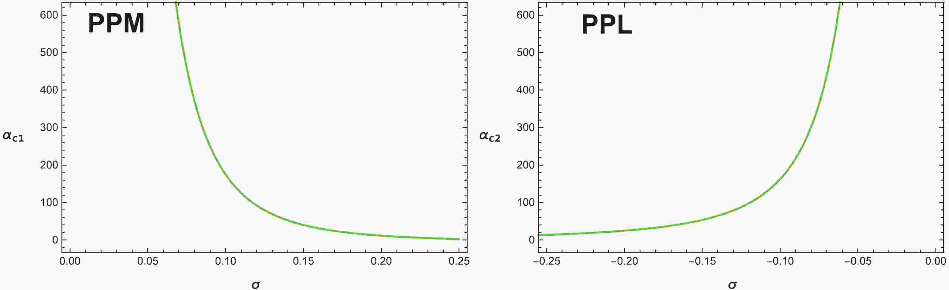
$r_{ps}$ , outside the event horizon. However, it is not easy to obtain the analytical form of the photon sphere radius,$r_{ps}$ , owing to the complexity of the coupled term associated to the Weyl tensor in Eq. (54). To avoid such complex problems and to obtain the radius,$r_{ps}$ , for the coupled photons, we apply numerical methods. Our outcomes demonstrate that the radius,$r_{ps}$ , of the photon sphere only occurs in the system when$\alpha_{c1}$ $>\alpha$ $>\alpha_{c2}$ both for the PPM and PPL cases. In comparison, for the coupled photons, the critical values can be resolved by the overlapping situation of the radius,$r_{ps}$ , with the event horizon. Moreover, there are critical values,$\alpha_{c1}$ for the PPM and$\alpha_{c2}$ for the PPL, which depend on the Kiselev parameter,$\sigma$ , and are defined as follows:$\begin{split}\alpha_{c1} =& -2\alpha_{c2} \\=& \frac{1}{8}\left[\frac{1+3(1-8\sigma M)^{\frac{1}{2}}+3(1-8\sigma M)+(1-8\sigma M)^{\frac{3}{2}}}{8\sigma^{3}M}\right].\end{split}$

(55) By setting
$E = 1$ , because the coupling parameter,$\alpha\rightarrow0$ , we find that the function,$W \rightarrow 1$ , which results in that the impact parameter and the equation of circular photon orbits for the PPL are the same as those for the PPM. This suggests that gravitational lensing is independent of the polarization directions of the photon in the case without the coupling. From Fig. 1, it is clear that the critical value,$\alpha_{c1}$ , decreases, and the critical value,$\alpha_{c2}$ , increases when$\sigma$ increases for both the PPM and PPL, respectively. Applying a numerical method, we present the dependence of the photon sphere radius,$r_{ps}$ , on the coupling parameter,$\alpha$ , and the Kiselev parameter,$\sigma$ , for the PPM and PPL, as shown in Figs. 2 and 3. We find that with the increase in$\alpha$ , the radius,$r_{ps}$ , increases for the PPL, whereas it decreases for the PPM. Meanwhile, when$\sigma$ increases, the radius,$r_{ps}$ , decreases for the PPL and increases for the PPM.
Figure 1. (color online) Variation in the critical values with Kiselev parameter
$\sigma$ at$M = 0.5$ . The photon sphere radius occurs only in the system when$\alpha$ $<\alpha_{c1}$ for the PPM and$\alpha$ $>\alpha_{c2}$ for the PPL, respectively.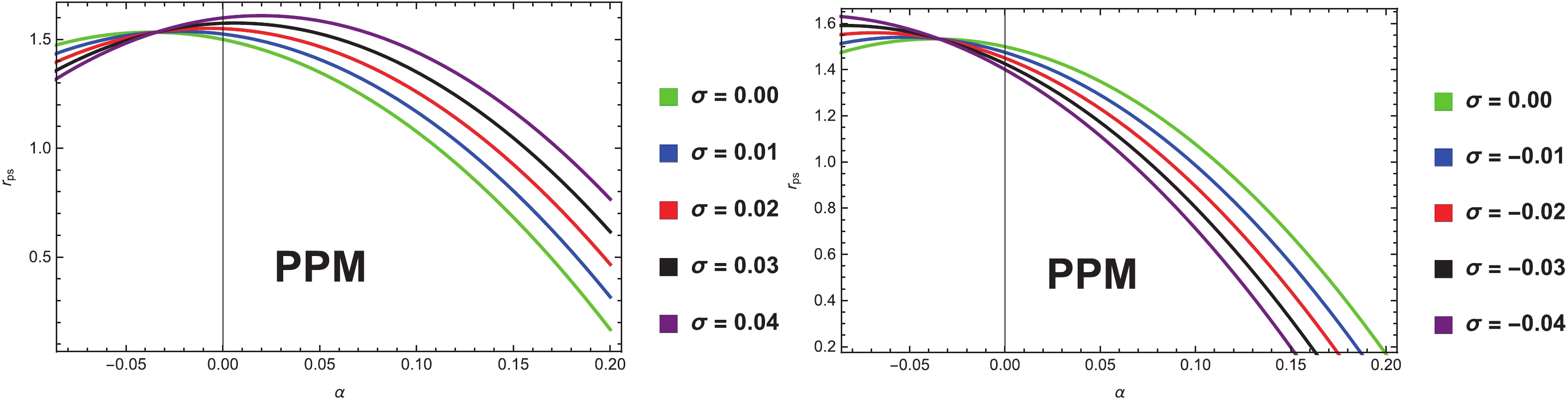
Figure 2. (color online) Variation in the photon sphere radius for the PPM with coupling parameter
$\alpha$ for different Kiselev parameters$\sigma$ , where$M = 0.5$ .
Figure 3. (color online) Variation in photon sphere radius for the PPL with coupling parameter
$\alpha$ for different Kiselev parameters$\sigma$ , where$M = 0.5$ .From Figs. 2 and 3, we see that the features of gravitational lensing are completely different for the PPL and PPM cases, respectively. In a different scenario, the gravitational lensing depends on the photon polarization drections with the coupling parameter and the Kiselev parameter.
-
Now, we discuss the following gravitational lensing observables in the Kieslev black Hole spacetime.
-
For a photon coupled to the Weyl tensor coming from infinity, the relation in (51) is limited on the equatorial plane; one can find that the deflection angle in the Kiselev black hole spacetime is similar to that in the case without the coupling [33]
$\alpha(r_{0}) = I(r_{0}) - \pi,$

(56) with
$I(r_{0}) = 2\int_{r_{0}}^{\infty} \frac{{\rm d}r}{\sqrt{\dfrac{A(r)C(r)}{W(r)}}\sqrt{\dfrac{C(r)A(r_{0})W(r_{0})}{A(r)W(r)C(r_{0})}-1}},$

(57) where the variable,
$r_{0}$ , is the closest approach distance, whereas$I(r_{0})$ depends on the polarization directions of the photons coupled to the Weyl tensor in a background spacetime. This suggests that the physical properties of the deflection angle for the PPM are different from those for the PPL. Moreover, we can use the method of approximation proposed by Bozza [42], which helps us to study the analytic features of the angle of deflection. For this, we have a new variable [83]$z = 1 - \frac{r_{0}}{r},$

(58) Therefore, Eq. (57) yields
$I(r_{0}) = \int_{0}^{1} R(z,r_{0})F(z,r_{0}){\rm d}z,$

(59) where
$R(z,r_{0}) = 2\frac{W(r)r^{2}\sqrt{C(r_{0})}}{r_{0}C(r)} = 2W(z,r_{0}),$

(60) $F(z,r_{0}) = \frac{1}{\sqrt{A(r_{0})W(r_{0})-\dfrac{A(z,r_{0})W(z,r_{0})C(r_{0})}{C(z,r_{0})}}}.$

(61) For all the values of
$r_{0}$ and z, functions$R(z,r_{0})$ are regular. Similarly, when$z\rightarrow 0$ , the other functions$F(z,r_{0})$ are divergent. Owing to this reason, the integral in (59) may be separated into two different types: one is divergent$I_{D}(r_{0})$ and the other part is regular$I_{R}(r_{0})$ with different polarizations, i.e.,$I_{D}(r_{0}) = \int_{0}^{1} R(0,r_{ps})F_{0}(z,r_{0}){\rm d}z,$

(62) $I_{R}(r_{0}) = \int_{0}^{1} [R(z,r_{o})F(z,r_{0}) - R(0,r_{ps})F_{0}(z,r_{0})]{\rm d}z,$

(63) whereas the new function,
$F_{0}(z,r_{0})$ , in (63) can be obtained by expanding the argument of the square root in$F_{0}(z,r_{0})$ to the second order in z as follows:$F_{0}(z,r_{0}) = \frac{1}{\sqrt{p(r_{0})z + q(r_{0})z^{2}}},$

(64) with
$\begin{split}p(r_{0}) =& - \frac{r_{0}}{C(r_{0})} \{W(r_{0})[A'(r_{0})C(r_{0}) - A(r_{0})C'(r_{0})] \\&+ A(r_{0})C(r_{0})W'(r_{0})\},\end{split}$

(65) $ \begin{split} q(r_{0}) = & \frac{r_{0}}{2C^{2}(r_{0})} \{2[C(r_{0}) - r_{0} C'(r_{0})][A(r_{0})W(r_{0})C'(r_{0})\\& - C(r_{0})(A(r_{0})W(r_{0}))'] + r_{0}C(r_{0})\\&\times[A(r_{0})W(r_{0})C''(r_{0}) - C(r_{0})(A(r_{0})W(r_{0}))'']\}. \end{split}$

(66) When the coefficient,
$p(r_{0})$ , is nonzero$(r_{0} \neq r_{ps})$ , the divergence order in$F_{0}(z,r_{0})$ is$1/\sqrt{z}$ , and it may be integrated to obtain the possible result. When$p(r_{0})$ is zero$(r_{0} = r_{ps})$ , the divergence becomes$1/z$ , which originates the integral as divergent. Hence, this shows that each photon that is captured by the central object, must have$r_{0} < r_{ps}$ . So, in this way, the photon cannot emerge back [42]. This suggests that in the strong gravitational limit field, because the photon is near to the photon sphere, the deflection angle diverges logarithmically for the coupled photons [42]. Hence,$\alpha(\theta) = - \bar{a} \log \left[\frac{\theta D_{1}}{u(r_{ps})} - 1\right] + \bar{b} + O[u - u(r_{ps})],$

(67) with
$ \begin{split} \bar{a} =& \frac{R(0,r_{ps})}{2\sqrt{q(r_{ps})}}, \\ b_{R} =& I_{R}(r_{ps}), \\\bar{b} =& - \pi + b_{R} + \bar{a} \log\left[\frac{2r_{hs}^2 u(r_{ps})''}{u(r_{ps})}\right], \end{split}$

(68) where
$D_{1}$ indicates the distance between the gravitational lens and the observer. The angle,$\theta = u/D_{1}$ is defined as the angular separation between the image and the lens [63]. Using the relations in (47) and (48) in (68), one can find the coefficients ($\bar{a}$ and$\bar{b}$ ) in the strong gravitational lensing formula in (67). The variation in the functions ($\bar{a}$ and$\bar{b}$ ) for the coupled photon with the coupling parameter,$\alpha$ , for the different Kiselev parameters,$\sigma$ are shown in Figs. 4-5. Moreover, from the relations in (67)-(68), we can study the physical properties of a strong gravitational lensing for a coupled photon in the Kiselev black hole spacetime. It is shown that both the coefficients ($\bar{a}$ and$\bar{b}$ ) depend not only on the polarization directions of the photon coupling with the Weyl tensor, but also on the Kiselev parameter. In Figs. 4-5, we plot the variation in the functions$(\bar{a}$ and$\bar{b})$ by a numerical approach with the coupling parameter for different Kiselev parameters. The function,$\bar{a}$ , constantly increases with the increase in the coupling parameter and the Kiselev parameter for the case of the PPM, whereas the function,$\bar{a}$ , decreases for the PPL with the increase in the coupling parameter, and increases when the Kiselev parameter increases, as shown in Fig. 4. The variation in$\bar{b}$ is more complex with the coupling parameter$\alpha$ for different Kiselev parameters$\sigma$ . For the PPM, the function,$\bar{b}$ , first decreases up to its minimum with the coupling parameter,$\alpha$ , for different values of$\sigma$ , and then increases up to its maximum with the further increase in the coupling parameter,$\alpha$ ; subsequently, it decreases again with the coupling parameter,$\alpha$ . Moreover, the variation in$\bar{b}$ with the coupling parameter,$\alpha$ , for the different values of the Kiselev parameter,$\sigma$ , for the PPL case is totally converse to that for the PPM, as shown in Fig. 5. Further, we see that as the coupling parameter,$\alpha$ , approaches to the critical values$(i.e., \alpha_{c1}$ or$\alpha_{c2})$ , the deflection angle can not remain valid in the system,$\alpha$ $>\alpha_{c1}$ for the case of PPM and$\alpha$ $<\alpha_{c2}$ for the PPL, in the strong deflection limit (67). Hence, with the existence of the coupling terms, the variation in the functions$(\bar{a}$ and$\bar{b})$ become more difficult. The reason is that the coupling effects depend not only on the$\alpha$ values but also on the coupled photon polarization directions. Moreover, the variation in the deflection angles for the PPM and PPL cases is also explored at$u = u_{ps} + 2$ , respectively (see Fig. 6). We investigate that the behaviors of the deflection angles are the same as those for the function,$\bar{a}$ , which shows that it can be evaluated by the experience that the deflection angles of the photons in the strong field limit are dominated by the logarithmic term.
Figure 4. (color online) Variation in the strong deflection limit function,
$\bar{a}$ , with the coupling parameter,$\alpha$ , for different Kiselev parameters,$\sigma$ , for the PPM and PPL cases, where$M = 0.5$ .
Figure 5. (color online) Variation in the strong deflection limit function,
$\bar{b}$ , with the coupling parameter,$\alpha$ , for different Kiselev parameters,$\sigma$ , for the PPM and PPL cases, where$M = 0.5$ .
Figure 6. (color online) Variation in the deflection angle,
$\alpha({\theta})$ , with the coupling parameter,$\alpha$ , for different Kiselev parameters,$\sigma$ , for the PPM and PPL cases, where$M = 0.5$ . -
We compute the essential relations to achieve the shape of the Kiselev black hole shadow, which suggests the study of motion of a test particle. Furthermore, to obtain the equation of motion, we use the Lagrangian and Hamiltonian Jacobi equation, which demands the study of the geodesic equation of a particle near the Kiselev spacetime. Hence, for describing the motion of the particle, the Lagrangian,
${\cal{L}}$ , is given as${\cal{L}} = g_{\mu\nu}\frac{{\rm d}x^{\mu}}{{\rm d}\lambda}\frac{{\rm d}x^{\nu}}{{\rm d}\lambda}.$

(69) Here, the canonically conjugate momenta for the metric in (11) have the following forms:
$P_{t} = f(r) \dot{t} = E,$

(70) $P_{r} = f(r)^{-1} \dot{r},$

(71) $P_{\theta} = r^{2}\dot{\theta} ,$

(72) $P_{\phi} = r^{2} \sin^{2}\theta \dot{\phi} = L,$

(73) where E is known as the energy and L defines the angular momentum per unit mass of the photon. To obtain circular photon orbits around a particular black hole, the Hamiltonian Jacobi technique is helpful, and also, we use the Hamiltonian Jacobi technique to formulate the geodesic equation by applying the Carter approach [84] for a Kiselev black hole. In this way, the Hamiltonian Jacobi equation can be written for a particular black hole in the following form:
$\frac{\partial S}{\partial\lambda} = {\cal{H}} = - \frac{1}{2}g^{\mu\nu}\frac{\partial S}{\partial x^{\mu}}\frac{\partial S}{\partial x^{\nu}},$

(74) where S denotes the action of the Jacobi, and using Eq. (11) in Eq. (74), we have
$\begin{split}- 2\frac{\partial S}{\partial\lambda} =& - \frac{1}{f(r)}\left(\frac{\partial S_{t}}{\partial t}\right)^2 + f(r ) \left(\frac{\partial S_{r}}{\partial r}\right)^2 \\&+ \frac{1}{r^2} \left(\frac{\partial S_{\theta}}{\partial \theta}\right)^2 + \frac{1}{r^2\sin^2 \theta}\left(\frac{\partial S_{\phi}}{\partial \phi}\right)^2.\end{split}$

(75) Now, we suppose two Killing fields
$\xi_{t,\phi} = \partial_{t,\phi}$ for simplicity; then the action of the Jacobi S takes the form,$S = \frac{1}{2}m^{2}_{p} \lambda - E t + S_{r}(r) + S_{\theta}(\theta) + L \phi,$

(76) where
$m_{p}$ is the test particle mass; for the photon, it is assumed to be zero.$S_{r}(r)$ and$S_{\theta}(\theta)$ both are functions of r and$\theta$ , respectively. Inserting Eq. (76) into Eq. (74), we obtain the complete equation of the null geodesic for the Kiselev black hole spacetime as$\dot{t} = \frac{E}{f(r)},$

(77) $r^2 \dot{r} = \pm\sqrt{R},$

(78) $r^2 \dot{\theta} = \pm\sqrt{\Theta},$

(79) $\dot{\phi} = \frac{L}{r^2\sin^2 \theta},$

(80) where signs
$\pm$ are used for the radial direction of the outgoing and ingoing particle motions, respectively [85]. Here, R and$\Theta$ are defined by$R = r^4 E^{2} - r^{2}\left(1 - \frac{2M}{r} - \sigma r\right)(L^{2} + {\cal{K}}), $

(81) $\Theta = {\cal{K}} - L^{2} \cot^{2} \theta,$

(82) where
${\cal{K}}$ is called the Carter constant. The effective potential,$V_{\rm eff}(r)$ , for an asymptotically non-flat spacetime in (11) is defined as follows:$V_{\rm eff}(r) = \frac{1}{r^{2}}\left(1 - \frac{2M}{r} - \sigma r\right)(L^{2} + {\cal{K}}) - E^{2}.$

(83) The unstable circular orbits constitute the photon sphere and define the boundary of the shadow cast by the compact body. These unstable circular orbits can be obtained by maximizing the effective potential,
$V_{\rm eff}(r)$ , which leads to$V_{\rm eff}(r) = \frac{\partial V_{\rm eff}(r)}{\partial r} = 0 \;\;\; {\rm or} \;\;\; R(r) = \frac{\partial R(r)}{\partial r} = 0.$

(84) For the general orbits, we consider two impact parameters
$\xi = \dfrac{L}{E}$ and$\eta = \dfrac{{\cal{K}}}{E^{2}}$ , which are functions of the constants of motion E, L, and${\cal{K}}$ . These impact parameters define the properties of the photons near a black hole. To visualize the black hole shadow more clearly, it is useful to adopt the celestial coordinates. Recently, Haroon et al. [86] introduced the technique for defining the celestial coordinates of an asymptotically non-flat spacetime; we follow this approach and find the following form of the modified celestial coordinates:$x = -\sqrt{1-\sigma}\xi {\rm csc}\theta,$

(85) $y = \pm\sqrt{1-\sigma}\sqrt{\eta - \xi^{2}\cot^{2}\theta},$

(86) For the equatorial plane,
$\theta = \dfrac{\pi}{2}$ , and Eqs. (85) and (86) are simplified as$x = -\sqrt{1-\sigma}\xi,$

(87) $y = \pm\sqrt{1-\sigma}\sqrt{\eta}.$

(88) Eqs. (87) and (88) yield the following relation:
$\begin{split}&x^{2} + y^{2} = (1-\sigma M)\\& \frac{(-2-5\sigma M+2\sqrt{1+6\sigma M})(-1+\sqrt{1+6\sigma M})^{3}}{\sigma^{2}(-1-2\sigma M+\sqrt{1+6\sigma M})(-3-8\sigma M+3\sqrt{1+6\sigma M})}.\end{split}$

(89) The contour based on Eq. (89) can describe the apparent shape of a Kiselev black hole. From Eq. (89), the size of a Kiselev black hole depends on the mass and the Kiselev parameter of the space-time. Eq. (89) governs the complete orbit of a photon around the black hole, which casts a shadow and appears as a circle. Now, we take the contour plot of Eq. (89), which shows the shadow of the Kiselev black hole, as clearly shown in Fig. 7. The size of the shadow cast by the Kiselev black hole increases with the increase in the Kiselev parameter and mass.

Figure 7. (color online) Shadow cast by the Kiselev black hole spacetime at
$\theta = \pi/2$ at different values of the Kiselev parameter,$\sigma$ , and the mass, M. -
The lens equation for the observer and the source can be written in the following form [43-45]
$\gamma = \frac{D_{1} + D_{2}}{D_{2}}\theta - \alpha(\theta) {\rm mod} 2\pi,$

(90) where
$\gamma$ defines the angle between the optical axis and the source direction,$D_{1}$ represents the distance of the observer and the lens,$D_{2}$ represents the distance of the source and the lens. Here, we take only the simplest case in which the observer, lens, and source are extremely arranged, so that the angular separation for the$n^{th}$ relativistic image and the lens may be defined as [43-45]$\theta_{n} \simeq \theta^{0}_{n}\left(1 - \frac{u_{ps}e_{n}(D_{1} + D_{2}) }{\bar{a}D_{1}D_{2}}\right),$

(91) and
$\theta^{0}_{n} = \frac{u_{ps}}{D_{1}}(1 + e_{n}), \;\;\;\;\; e_{n} = {\rm e}^{\textstyle\frac{\bar{b} + |\gamma| - 2 \pi n}{\bar{a}}},$

(92) where the position of the image alternate to
$\alpha = 2n\pi$ is$\theta^{0}_{n}$ and n is any integer. If$n\rightarrow \infty$ , we obtain the relation,$e_{n}\rightarrow 0$ . This relation provides a result for the impact parameter,$u_{ps}$ , distance$D_{1}$ , and a set of images,$\theta_{\infty}$ , which can be defined as$u_{ps} = D_{1}\theta_{\infty}.$

(93) We investigate that the strong-deflection limit functions,
$\bar{a}$ and$\bar{b}$ , which can be obtained if there exist extra two observations. Thus, as in [42-45], we suppose a perfect situation where the outermost image,$\theta_{1}$ is separated as a single image and all the remaining ones are packed together in the relativistic images,$\theta_{\infty}$ . In this way, the angular separation, s, and the relative magnitudes,$r_{m}$ , among the first image and other ones may be further defined as$s = \theta_{1} - \theta_{\infty} = \theta_{\infty}{\rm e}^{\textstyle\frac{\bar{b} - 2\pi}{\bar{a}}},$

(94) $r_{m} = 2.5 \log R_{0} = 2.5 \log \left(\frac{\mu_{1}}{\sum^{\infty}_{n = 2}\mu_{n}}\right) = \frac{ 5 \pi}{\bar{a}}\log e,$

(95) where
$R_{0}$ is a flux ratio between the first image and all the other images. By adopting all these observations ,such as s,$r_{m}$ , and$\theta_{\infty}$ , it is easy to evaluate$\bar{a}$ ,$\bar{b}$ , and$u_{ps}$ in the limit of a strong deflection. For the existence of that coupling in our universe, we compare the values of these observations to those of the observations that are predicted by the theoretical models of coupling. Using this technique it is easy to store the characteristics information in a strong gravitational lensing. However, the distance of our galaxy is approximately 8.5 kpc [63] taken from the earth. So, the ratio becomes GM/D1 ≈ 2.4734×10⁻¹¹, and the galactic central object mass is approximately evaluated to be$4.4 \times 10^{6} M_{\odot}$ . The situation of the photon coupling with the Weyl tensor in the Kiselev spacetime shows that the values of the strong-deflection limit functions$(\bar{a}, \bar{b})$ and other possible observables can easily be estimated numerically in a strong gravitational lensing by solving Eqs. (68), (93), (94), and (95). In Figs. 8–10, we plot the dependence of observables$\theta_{\infty}$ , s, and$r_{m}$ for different values of the Kiselev parameter,$\sigma$ , on the coupling constant,$\alpha$ . We observe that for the case of the PPL, the angular positions of observables$\theta_{\infty}$ and$r_{m}$ are increasing functions of the coupling constant,$\alpha$ , but decreasing functions of different values of$\sigma$ . On the other hand, in the case of the PPM, the angular positions of$\theta_{\infty}$ and$r_{m}$ the directly decreasing functions of both parameters$\alpha$ and$\sigma$ , as shown in Figs. 8 and 10, respectively. The variation in the angular separation, s, is given in Fig. 9, where we see that for the PPM case, observable s increases directly with$\alpha$ and$\sigma$ , whereas in the PPL, this angular separation decreases with$\alpha$ and increases with$\sigma$ , respectively.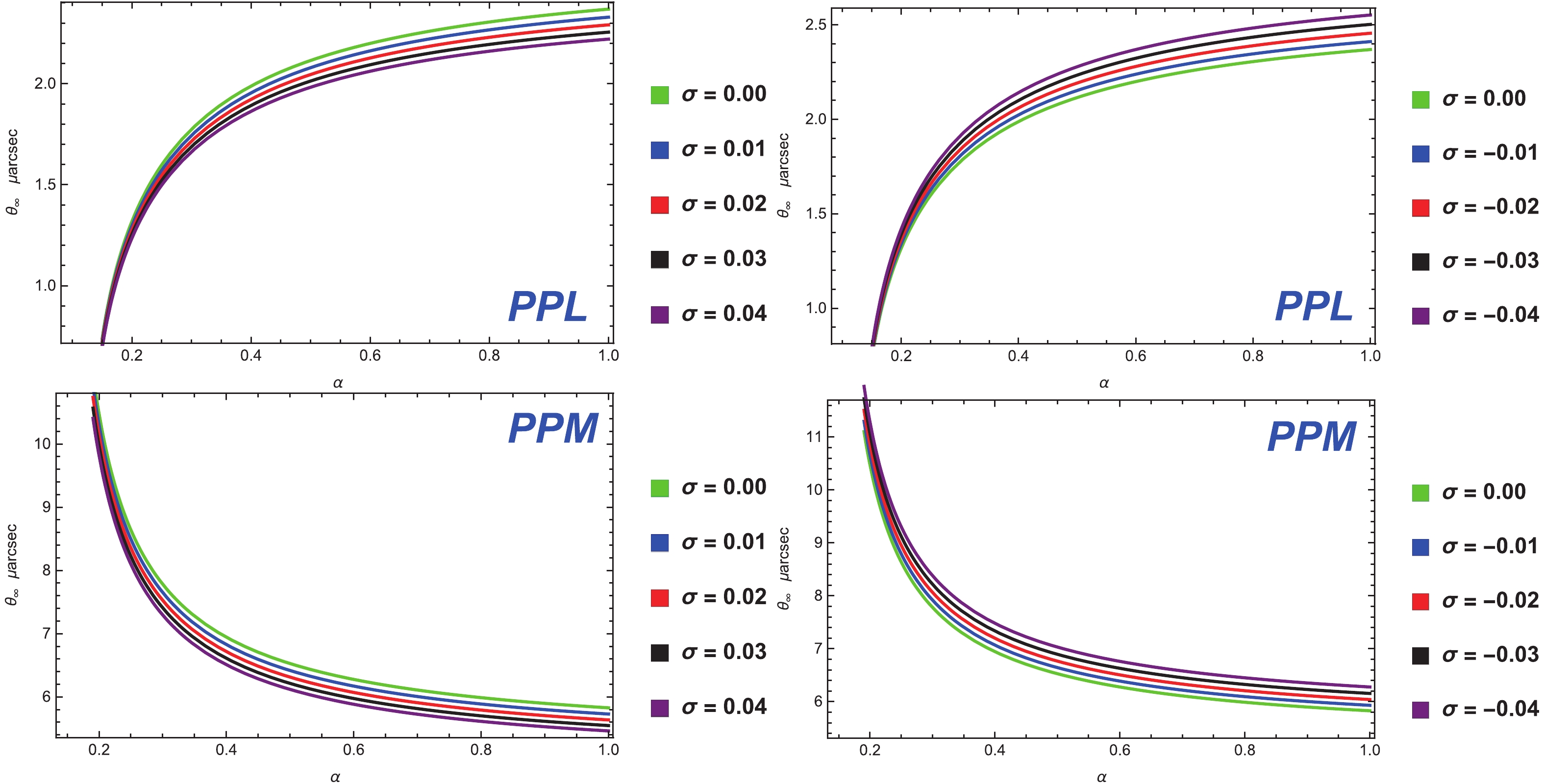
Figure 8. (color online) Variation of the innermost relativistic image,
$\theta_{\infty}$ , with the coupling parameter,$\alpha$ , for different Kiselev$\sigma$ for the cases of the PPL and PPM, where$M = 0.5$ .
Figure 9. (color online) Variation in the angular separation, s, with the coupling parameter,
$\alpha$ , for different Kiselev$\sigma$ for the cases of the PPM and PPL, where$M = 0.5$ .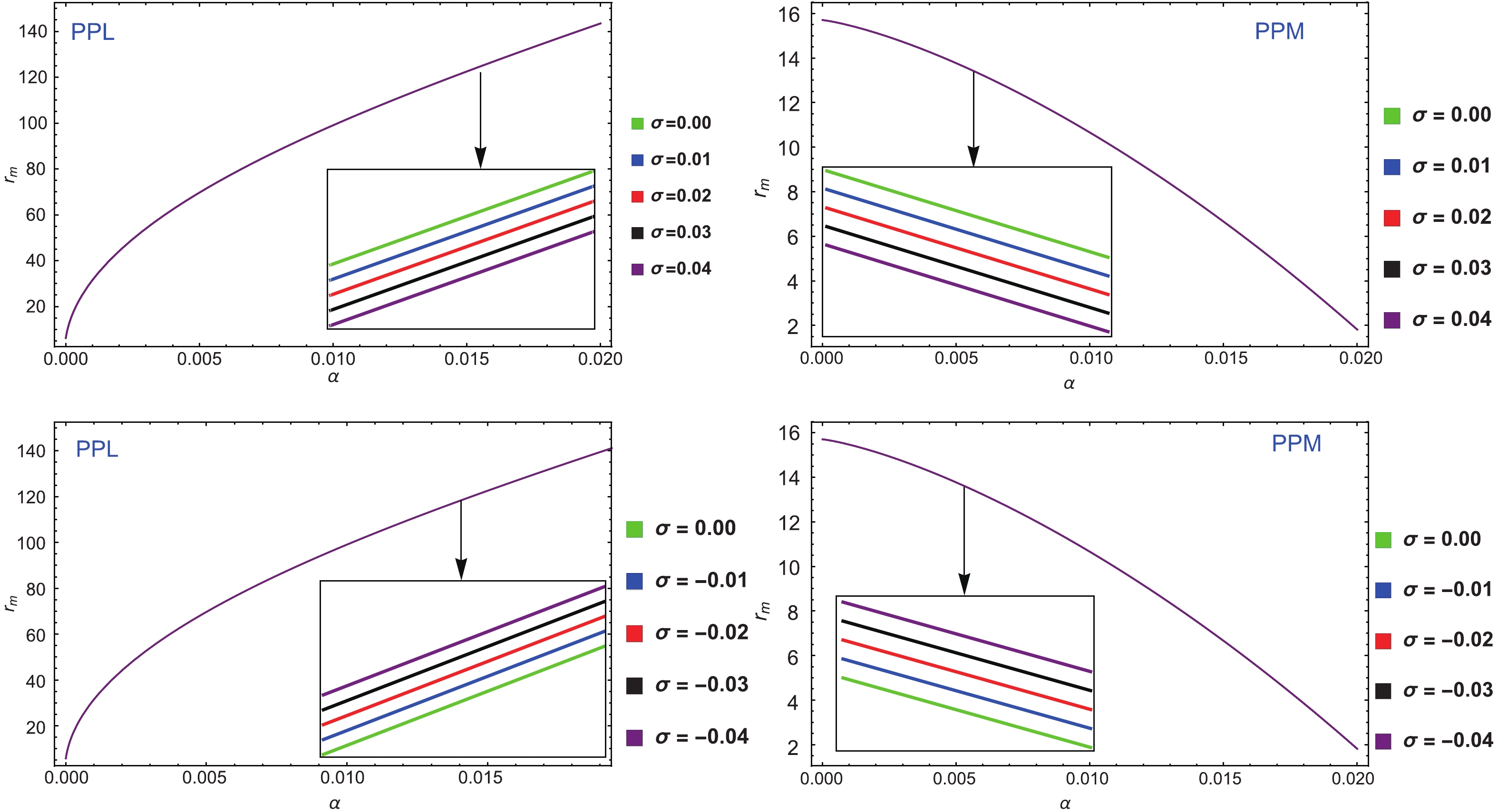
Figure 10. (color online) Variation in the relative magnitude,
$r_{m}$ , with the coupling parameter,$\alpha$ , for different Kiselev parameter$\sigma$ for the cases of the PPL and PPM, where$M = 0.5$ . -
This paper deals with the dynamical equation of photons coupled to the Weyl tensor and the strong gravitational lensing in the Kiselev black hole spacetime. We find that the coupling parameter,
$\alpha$ , Kiselev parameter$\sigma$ , and the polarization directions are important for the advancement of the coupled photons. These parameters also contribute significantly to explaining the photon sphere radius,$r_{ps}$ , angle of deflection, and coefficients$\bar{a}$ and$\bar{b}$ appearing in the lensing formula. The modified light cone conditions suggest that in this spacetime, the photons travel along null geodesics. Here, we conclude that when$\sigma$ tends to zero in Eq. (11), critical value$\alpha_{c1} = M^{2}$ for the PPM and critical value$\alpha_{c2} = \dfrac{-M^{2}}{2}$ for PPL, which are consistent with those in the Schwarzschild black hole spacetime [63]. From the equation of circular photon orbits, the radius,$r_{ps}$ , for the PPM decreases monotonously with the coupling parameter,$\alpha$ , whereas in the case of the PPL, we find that$r_{ps}$ increases monotonously with$\alpha$ . For the PPM, the monotonicity of$r_{ps}$ gradually increases with$\sigma$ , and for the PPL, the monotonicity of$r_{ps}$ gradually decreases with$\sigma$ , which is different from that in the Schwarzschild case [63]. The gravitational lensing formula functions,$\bar{a}$ and$\bar{b}$ , are given in Figs. 4 and 5, and we see that with the increase in$\alpha$ , the function,$\bar{a}$ , increases for the PPM, whereas$\bar{a}$ decreases with$\alpha$ for the PPL. The function,$\bar{b}$ , for the case of the PPM, first decreases to its minimum with$\alpha$ and then increases to its maximum with further increase in$\alpha$ ; after that, it decreases with$\alpha$ again. Meanwhile, for the PPL, the function,$\bar{b}$ , first increases to its maximum with$\alpha$ and then decreases to its minimum with further increase in$\alpha$ ; after that, it increases with$\alpha$ again. For the PPM, the monotonicity of$\bar{a}$ directly increases respectively with$\sigma$ for the PPM and PPL, which is different from that in the Schwarzschild case [63]. Moreover, the variation in$\bar{b}$ with the coupling parameter,$\alpha$ , for the different values of the Kiselev parameter,$\sigma$ , for the case of the PPL is totally converse to that for the PPM. The strong gravitational lensing,$\alpha(\theta)$ , has similar behaviors of the function,$\bar{a}$ . We obtain the shadow cast in the Kiselev black hole spacetime, where the size of the shadow is an increasing function of both the mass, M, and the Kiselev parameter,$\sigma$ . The variation in the angular separation, s, with the coupling parameter,$\alpha$ , is converse to the variations in the relativistic images,$\theta_{\infty}$ , and the relative magnitude,$r_{m}$ , with the coupling parameter,$\alpha$ . The changes in these observables with$\alpha$ also depend on the value of the Kiselev parameter,$\sigma$ . In the typical Kiselev black hole spacetime, the observables,$\theta_{\infty}$ , and the relative magnitude,$r_{m}$ , decreases with$\sigma$ , but s increases, which is different from that in the Schwarzschild case [63].We are grateful to the scholarly anonymous referees for their efforts and valuable suggestions for improving this manuscript.
Strong gravitational lensing for photon coupled to Weyl tensor in Kiselev black hole
- Received Date: 2020-02-28
- Available Online: 2020-09-01
Abstract: The objective of the present work is to highlight the phenomena of strong gravitational lensing and deflection angle for the photon coupling with the Weyl tensor in a Kiselev black hole. Here, we have extended the prior work of Chen and Jing (S. Chen and J. Jing, JCAP, 10: 002 (2015)) for a Schwarzschild black hole to a Kiselev black hole. For this purpose, the equation of motion for the photons coupled to the Weyl tensor, null geodesic, and equation of photon sphere in a Kiselev black hole spacetime have been formulated. It is found that the equation of motion of the photons depends not only on the coupling between the photons and the Weyl tensor, but also on the polarization direction of the photons. There is a critical value of the coupling parameter,


 DownLoad: