


 Abstract
 HTML
HTML Reference
 Related
 PDF
PDF


-
The single-particle resonant states in the continuum play crucial roles in the formation of halos in exotic nuclei [1]. For example, studies by the relativistic continuum Hartree-Bogoliubov theory suggested that giant halos can be formed in the neutron-rich Zr and Ca isotopes if more than two valence neutrons occupy the resonant states with low angular momentums [2, 3], and the existence of a possible deformed halo in
$ ^{40,42}{\rm{Mg}} $ and$ ^{22}{\rm{C}} $ is mainly decided by the single-particle states around the Fermi surface, including the resonant states in the continuum [4-7]. Consequently, the exploration of resonant states is becoming increasingly important, attracting further attention.During the past years, a series of approaches have been taken or developed in the exploration of the single-particle resonant states. Some approaches are based on the conventional scattering theories, such as R-matrix theory [8, 9], K-matrix theory [10], S-matrix theory [11, 12], Jost function approach [13, 14], and the scattering phase shift (SPS) method [11, 15, 16]. Further, some techniques that are used for bound states have also been extended to study the single-particle resonant states, such as the complex momentum representation (CMR) method [17-19], the complex scaling method (CSM) [20-28], complex-scaled Green's function (CGF) method [29-31], real stabilization method (RSM) [32], and analytical continuation of the coupling constant (ACCC) method [33-45].
The Green's function (GF) method [46-49] is likewise a successful candidate for studying resonances, as it can treat the continuum exactly. With this method, the single-particle spectrum covering the bound states and the continuum are treated on the same footing, and exact energies and widths can be obtained for resonant states of all kinds. The correct asymptotic behaviors are well maintained for the density distributions. Further, GF is highly convenient to combine with nuclear models. Consequently, the GF method has been used extensively in the study of the nuclear structure and excitations. For example, by applying the GF method to the Hartree-Fock-Bogoliubov (HFB) theory in the coordinate representation, halos in both spherical and deformed nuclei are efficiently described [50-53]. Besides, the continuum quasiparticle random-phase approximation (QRPA) formulated with Green's function method [54] is developed to describe numerous interesting phenomena, such as the collective excitations [55-61], monopole pair vibrational modes and associated two-neutron transfer amplitudes [62], and neutron capture reactions [63].
The covariant density functional theory (CDFT) [64-67] has remarkable achievements in describing numerous systems and interesting phenomena, such as stable and exotic nuclei [68-71], hypernuclei [72-75], neutron stars [76, 77], pseudospin symmetries [78-81], and r-process simulations [82-84]. Thus, in recent years, we applied the Green's function method to the framework of the covariant density functional theory. In 2014, the relativistic mean field theory formulated with the Green's function method (RMF-GF) is developed, and as the first time, it is successfully applied to study the single-neutron resonant states [85]. It is also confirmed to be effective for the proton and
$ \Lambda $ -hyperon single-particle resonant states [86, 87]. In 2016, the relativistic continuum Hartree-Bogoliubov theory combining the Green's function method (RCHB-GF) is developed by containing the pairing correlation, which can describe the halos very well [88]. Very recently, Green's function method is further extended to study the resonances in deformed nuclei by solving a coupled-channel Dirac equation with quadrupole-deformed Woods-Saxon potential [89].In our previous studies [85-87], single-particle resonances were identified by comparing the density of states (DOS) displayed by nucleons moving in the mean-field potential with that of free particles. According to the DOS difference between the nucleons and free particles, the energy and width of resonant state are given by the position and the full-width at half-maximum (FWHM) of the resonant peak, respectively. In this approach, energies and widths can be obtained easily for narrow resonances with good accuracy. However, the accuracy decreases for the wide resonances due to the irregular shape of resonant peaks. In our recent study [89], a direct but very effective approach was proposed to investigate the resonant states by searching for the extremes of the GF in terms of resonant states that are poles located in the fourth quadrant of the complex energy plane. In this study, we applied this new approach with the GF method to study the single-particle resonances based on the RMF theory.
The paper is organized as follows. In Sec. 2, the GF method is briefly described. In Sec. 3, numerical details are presented. After the results and discussions in Sec. 4, a brief summary is given in Sec. 5.
-
In the RMF-GF theory [85], the GF is applied in the coordinate space to calculate the densities for nucleons and the single-particle spectrum of the Dirac equation. The Dirac equation for nucleons in the RMF theory [64-66] is
$ [{{\alpha}}\cdot{{p}}+V({{r}})+\beta(M+S({{r}}))]\psi_n({{r}}) = \varepsilon_n\psi_n({{r}}), $

(1) with the nucleon mass given by M, the Dirac matrices
$ {{\alpha}} $ and$ \beta $ , and the scalar and vector potentials$ S({{r}}) $ and$ V({{r}}) $ , respectively.A relativistic single-particle Green's function
$ {\cal G}({{r}},{{r'}};\varepsilon) $ satisfying the following definition needs to be constructed,$ [\varepsilon-\hat{h}({{r}})]{\cal G}({{r}},{{r}}';\varepsilon) = \delta({{r}}-{{r}}'), $

(2) with
$ \hat{h}({{r}}) $ denoting the Hamiltonian of the Dirac Eq. (1). Starting from Eq. (2) and taking a complete set of eigenstates$ \psi_{n}({{r}}) $ and eigenvalues$ \varepsilon_{n} $ , the GF is represented as$ {\cal G}({{r}},{{r}}';\varepsilon) = \sum\limits_n\frac{\psi_{n}({{r}})\psi_{n}^{\dagger}({{r}}')}{\varepsilon-\varepsilon_{n}}, $

(3) which has the form of a
$ 2\times2 $ matrix due to the two components of the Dirac spinor$ \psi_{n}({{r}}) $ ,$ {\cal G}({{r}},{{r}}';\varepsilon) = \left( \begin{array}{cc} {\cal G}^{(11)}({{r}},{{r}}';\varepsilon) & {\cal G}^{(12)}({{r}},{{r}}';\varepsilon) \\ {\cal G}^{(21)}({{r}},{{r}}';\varepsilon) & {\cal G}^{(22)}({{r}},{{r}}';\varepsilon) \end{array} \right). $

(4) Notably, the eigenvalues
$ \varepsilon_{n} $ of Dirac equation are poles of the Green's function in Eq. (3). Consequently, the eigenvalues$ \varepsilon_{n} $ can be obtained by searching for the poles of the GF. In practice, according to Ref. [49], this can be done with the help of the density of states (DOS)$ n(\varepsilon) $ ,$ n(\varepsilon) = \sum\limits_n\delta(\varepsilon-\varepsilon_{n}), $

(5) which displays similar discrete
$ \delta $ -function peaks for bound states at the eigenvalues$ \varepsilon = \varepsilon_{n} $ and distributes continuously in the continuum with peaks for resonances. DOSs$ n(\varepsilon) $ in a wide energy range is calculated by scanning the single-particle energy$ \varepsilon $ . Notably, for the continuum, energies$ \varepsilon $ are complex$ \varepsilon = \varepsilon_r+{\rm i}\varepsilon_i $ , and the energies for the resonant states can be written as$ \varepsilon_n = E-{\rm i}\Gamma/2 $ with the resonance energy E and width$ \Gamma $ .Taking the imaginary part of the GF, the DOSs can be calculated by the integrals in the coordinate
$ { r} $ space [85]. For the bound states, this is$ \begin{split} n(\varepsilon) =& -\dfrac{1}{\pi}\int {\rm d}{{r}}{\rm{Im}}[{\cal G}^{(11)}({{r}},{{r}};\varepsilon+{\rm i}\epsilon)\\&+{\cal G}^{(22)}({{r}},{{r}};\varepsilon+{\rm i}\epsilon)], \end{split} $

(6) where “
$ {\rm i}\epsilon $ ” is the introduced positive infinitesimal imaginary part to the single-particle energy$ \varepsilon $ , with which the$ \delta $ -function shaped DOSs for bound states are simulated by Lorentzian functions with the FWHM of$ 2\epsilon $ . For the resonant states, the infinitesimal imaginary part “$ {\rm i}\epsilon $ ” does not need to be introduced, as the single-particle energy$ \varepsilon $ is complex. Further, when scanning the imaginary part of complex energy$ \varepsilon_i $ before and after it had crossed the resonant states, it is found that the DOSs$ n(\varepsilon) $ differ by a minus sign. The DOSs for the resonant states can be written as$\begin{split} n(\varepsilon ) =&{ \delta ({\varepsilon _r} - E)}\\ =&{ \left\{ {\begin{array}{*{20}{l}} { - \dfrac{1}{\pi }\displaystyle\int {\rm d} {{r}}{\rm{Im}}[{{\cal{G}}^{(11)}}({{r}},{{r}};\varepsilon ) + {{\cal{G}}^{(22)}}({{r}},{{r}};\varepsilon )],}\\ {\;\;\;\;\;\;\;\;\;\;\;\;\;\;\;\;\;\;\;\;\;\;{\rm{if}}\;{\varepsilon _i} > - \Gamma /2,}\\ {\;\;\;\dfrac{1}{\pi }\displaystyle \int {\rm d} {{r}}{\rm{Im}}[{{\cal{G}}^{(11)}}({{r}},{{r}};\varepsilon ) + {{\cal{G}}^{(22)}}({{r}},{{r}};\varepsilon )],}\\ {\;\;\;\;\;\;\;\;\;\;\;\;\;\;\;\;\;\;\;\;\;\;\;{\rm{if}}\;{\varepsilon _i} < - \Gamma /2.} \end{array}} \right.} \end{split}$

(7) In practice, we calculate DOSs for resonances by scanning the entire complex energy range taking the first equation in Eq. (7), and they will reverse and become negative when
$ \varepsilon_i $ is over the resonant states. According to those changes, the widths of resonant states$ \Gamma/2 $ can be determined.In the spherical case, the GF can be expanded as
$ {\cal G}({ r},{ r'};\varepsilon) = \sum\limits_{\kappa m}Y_{\kappa m}(\theta,\phi)\frac{{\cal G}_{\kappa}(r,r';\varepsilon)}{rr'}Y_{\kappa m}^{*}(\theta',\phi'), $

(8) where
$ Y_{\kappa m}(\theta,\phi) $ is the spin spherical harmonic,$ {\cal G}_{\kappa}(r,r';\varepsilon) $ denotes the radial GF, and the quantum number$ \kappa $ labels different partial waves, which can provide the values of the angular momentums l and j,$ \left\{ \begin{array}{*{20}{l}} l = \kappa,\;\;j = \kappa-\dfrac{1}{2}, & {{\rm{if}}\; \kappa>0,} \\ l = -\kappa-1,\;\;j = -\kappa-\dfrac{1}{2}, & {{\rm{if}}\; \kappa<0.} \end{array} \right. $

(9) Then, the DOS for each partial wave
$ \kappa $ is$ \begin{split} n_{\kappa}(\varepsilon) =& -\frac{2j+1}{\pi}\int {\rm d}r{\rm{Im}}\left[{\cal G}_{\kappa}^{(11)}(r,r;\varepsilon) +{\cal G}_{\kappa}^{(22)}(r,r;\varepsilon)\right]. \end{split} $

(10) Practically, we perform the integrals in Eq. (10) in a finite box and obtain an approximate DOS
$ n_{\kappa}^{R}(\varepsilon) $ for a fixed$ R_{\rm {box}} $ .Finally, a Green's function
$ {\cal G}_{\kappa}(r,r';\varepsilon) $ with angular momentum$ \kappa $ and complex single-particle energy$ \varepsilon $ is constructed as [47]$ \begin{split} {\cal G}_{\kappa}(r,r';\varepsilon) = &\frac{1}{W_{\kappa}(\varepsilon)}\left[\theta(r-r')\phi^{(2)}_{\kappa}(r,\varepsilon)\phi^{(1)\dagger}_{\kappa}(r',\varepsilon)\right. \\ &\left.+\theta(r'-r)\phi^{(1)}_{\kappa}(r,\varepsilon)\phi^{(2)\dagger}_{\kappa}(r',\varepsilon)\right], \end{split} $

(11) where
$ \theta(r-r') $ is the step function,$ \phi^{(1)}_{\kappa}(r,\varepsilon) $ and$ \phi^{(2)}_{\kappa}(r,\varepsilon) $ are two linearly independent Dirac spinors$ \begin{split} \phi^{(1)}_{\kappa}(r,\varepsilon) =& \left( \begin{array}{c} g^{(1)}_{\kappa}(r,\varepsilon) \\ f^{(1)}_{\kappa}(r,\varepsilon) \end{array} \right),\\ \phi^{(2)}_{\kappa}(r,\varepsilon) = &\left( \begin{array}{c} g^{(2)}_{\kappa}(r,\varepsilon) \\ f^{(2)}_{\kappa}(r,\varepsilon) \end{array} \right), \end{split} $

(12) obtained by the Runge-Kutta integrals in the whole r space from the asymptotic behaviors of the Dirac spinors at
$ r\rightarrow0 $ and$ r\rightarrow\infty $ , respectively, and$ W_{\kappa}(\varepsilon) $ is the r-independent Wronskian funciton defined by$ W_{\kappa}(\varepsilon) = g^{(1)}_{\kappa}(r,\varepsilon)f^{(2)}_{\kappa}(r,\varepsilon)-g^{(2)}_{\kappa}(r,\varepsilon)f^{(1)}_{\kappa}(r,\varepsilon). $

(13) Exact asymptotic behaviors in the origin and at infinity are taken for the Dirac spinor. In particular, this is regular at
$ r\rightarrow 0 $ and satisfies$ \begin{array}{*{20}{l}} \phi^{(1)}_{\kappa}(r,\varepsilon) &\longrightarrow& r\left( \begin{array}{c} j_l(k r) \\ \dfrac{\kappa}{|\kappa|}\dfrac{\varepsilon-V-S}{k}j_{\tilde{l}}(kr)\\ \end{array} \right), \end{array} $

(14) where
$ \tilde{l} = l+(-1)^{j+l-1/2} $ is the angular momentum of the small component of the Dirac spinor,$k = $ $ \sqrt{(\varepsilon-V-S)(\varepsilon-V+S+2M)} $ is the single-particle momentum for all states, and the spherical Bessel function of the first kind$ j_l(k r) $ satisfies$ j_l(k r)\longrightarrow \frac{(kr)^l}{(2l+1)!!},\; \; \; {\rm{ when}}\; \; r\rightarrow 0. $

(15) The Dirac spinor at
$ r\rightarrow\infty $ behaves exponentially, decaying for the bound states while oscillating outgoing for the continuum, which can be written uniformly as,$ \begin{array}{*{20}{l}} \phi^{(2)}_{\kappa}(r,\varepsilon) &\longrightarrow&\left( \begin{array}{c} rk h^{(1)}_l(k r) \\ \dfrac{\kappa}{|\kappa|}\dfrac{rk^2}{\varepsilon+2M}h^{(1)}_{\tilde{l}}(k r) \\ \end{array} \right), \end{array} $

(16) with the single-particle momentum
$ k = \sqrt{\varepsilon(\varepsilon+2M)} $ and the spherical Hankel function of the first kind$ h^{(1)}_l(k r) $ . -
In this study, we aimed to compare the results with those obtained by previous GF calculations [85] and also those obtained by CMR [18], CSM [25], RSM [32], and ACCC [39] methods. We take the same nucleus
$ ^{120} {\rm{Sn}}$ as an example and investigate the single-particle resonant states for neutrons by taking the GF method based on the RMF theory. The energies, widths, and the density distributions in coordinate space for resonant states are given and compared with other methods. Both PK1 [90] and NL3 [91] parameters are taken in these RMF calculations.The equations in the RMF-GF theory are solved in the coordinate space, with different space sizes
$ R_{\rm{box}} $ and a step of d$ r = 0.1 $ fm. In Eq. (6), the infinitesimal imaginary parameter$ \epsilon $ is taken as$ 1\times 10^{-6} $ MeV when calculating DOSs for bound states. When calculating the DOSs$ n_{\kappa}^{R}(\varepsilon) $ by scanning energies$ \varepsilon $ in the fourth quadrant of the complex energy plane, the energy steps d$ \varepsilon $ is taken as$ 1\times10^{-4} $ MeV for both the real and imaginary energy components in the search for resonances. Consequently, the energies and widths of the resonant states predicted by the GF method have an accuracy of$ 0.1 $ keV. Further, significantly higher accuracy can be easily achieved by taking smaller energy steps d$ \varepsilon $ . -
The resonant states are well known as poles located in the fourth quadrant of the single-particle complex energy plane. Therefore, in this work, we take a direct approach to explore for these poles which are also the extremes of GF according to Eq. (3). In practice, the definition of density of states in Eq. (7) is applied and a series of DOSs
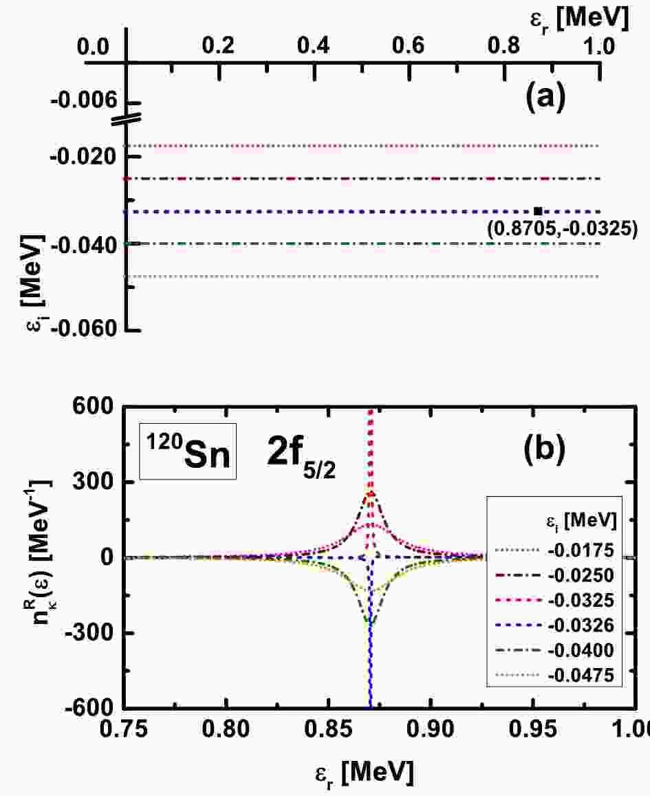
$ n_{\kappa}^{R}(\varepsilon) $ will be calculated by scanning the complex energy$ \varepsilon $ in the fourth quadrant, both in the directions of the real energy$ \varepsilon_{r} $ axis and the imaginary energy$ \varepsilon_i $ axis.As an example, in Fig. 1, we provide the details in determining the single-neutron resonant state
$ 2f_{5/2} $ in$ ^{120} {\rm{Sn}}$ . To explore the pole corresponding to the resonant state, as shown in Fig. 1(a), the complex energy$ \varepsilon $ in a wide range containing both the real$ \varepsilon_{r} $ and imaginary$ \varepsilon_{i} $ components are covered to calculate the DOSs. The PK1 effective interaction and the coordinate space of$ R_{\rm {box}} = 20\; $ fm are considered in the RMF-GF calculations. In Fig. 1(b), the calculated DOSs are plotted as functions of$ \varepsilon_{r} $ for different$ \varepsilon_i $ . In particular, with the imaginary energy$ \varepsilon_i $ varying from$ -0.0175\; $ MeV to$ -0.0475\; $ MeV, the DOSs alter significantly in the energy range from$ \varepsilon_r = 0.75\; $ MeV to$ 1.00\; $ MeV. With the imaginary energy$ \varepsilon_i $ approaching$ -0.0325 $ MeV, the peaks of DOS evolve to become increasingly sharper and finally reach the extreme. A peak in the shape of the$ \delta $ -function is located at$ \varepsilon_r = 0.8705\; $ MeV. Further, just after$ \varepsilon_i $ crossing the energy$ -0.0325 $ MeV, the peak of DOS reverses sharply. Subsequently, the peak of DOS evolves in an opposite way and becomes increasingly lower with$ \varepsilon_i $ reaching farther. This indicates a pole located at$ \varepsilon = 0.8705- {\rm i}0.0325\; $ MeV.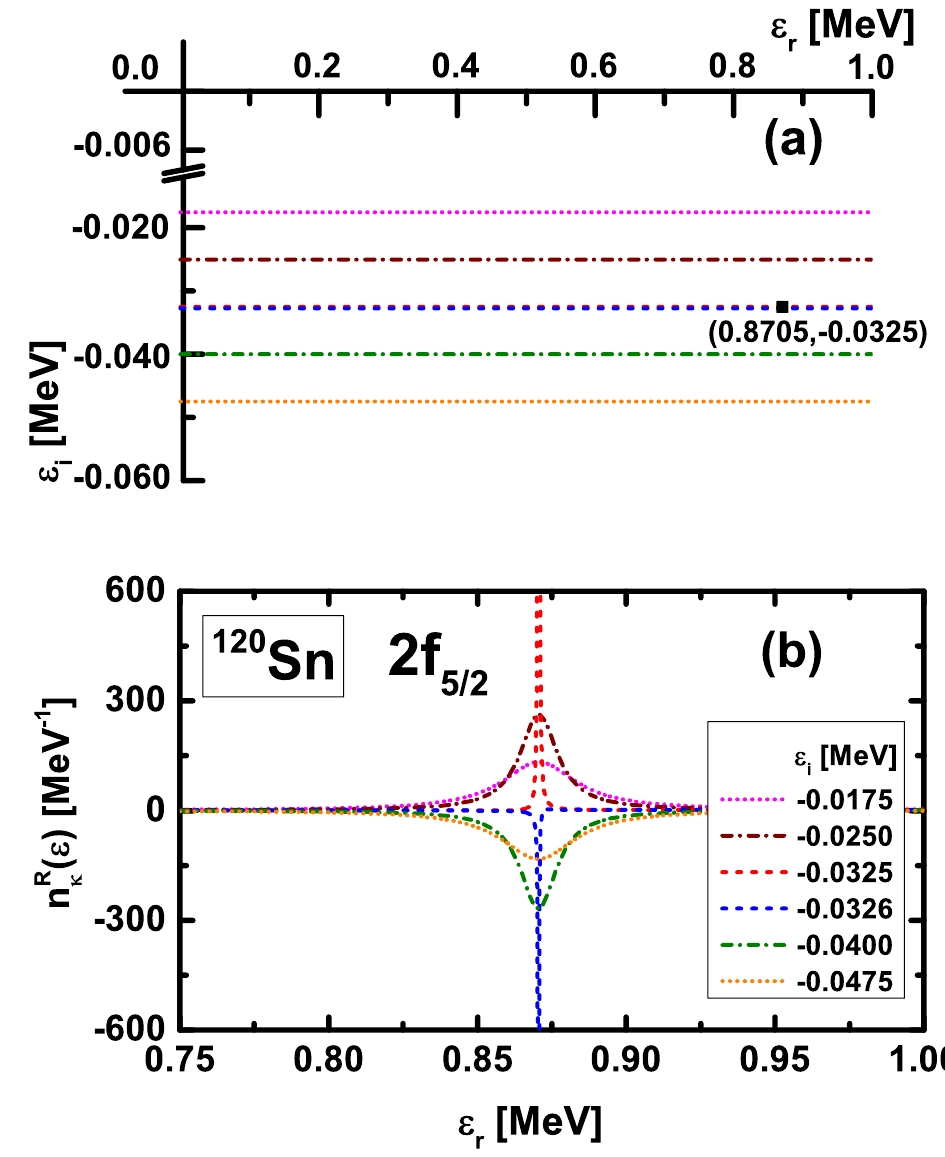
Figure 1. (color online) (a) Single-particle complex energy plane
$ \varepsilon = \varepsilon_r+{\rm i}\varepsilon_i $ and single-neutron resonant state$ 2f_{5/2} $ in$ ^{120} {\rm{Sn}}$ located in the fourth quadrant. (b) DOSs$ n_{\kappa}^{R}(\varepsilon) $ as functions of the complex energy$ \varepsilon $ including the real part$ \varepsilon_r $ and the imaginary part$ \varepsilon_i $ , obtained by the RMF-GF method by taking the PK1 effective interaction and space size$ R_{\rm {box}} = 20 $ fm.In the following, we verify the dependence of the obtained resonance energy and width
$ E-{\rm i}\Gamma/2 $ on the space size, as they must be constant against the changes of the coordinate space size$ R_{\rm {box}} $ . In Fig. 2, DOSs calculated by taking different coordinate space sizes$ R_{\mathrm{box}} = 20 $ (a),$ 25 $ (b), and$ 30 $ fm (c) are plotted for the single-neutron resonant state$ 2f_{5/2} $ in$ ^{120} {\rm{Sn}}$ . Notably, the shapes of DOSs for$ 2f_{5/2} $ in different$ R_{\rm {box}} $ are quite similar, and all of them reach the extreme at$ \varepsilon_i = -0.0325 $ MeV and reverse immediately at the following energy point$ -0.0326 $ MeV. Further, the peak of DOS in each case is located at the same energy$ \varepsilon_r = 0.8705\; $ MeV. Accordingly, we conclude that the energy and width of the resonant state$ 2f_{5/2} $ obtained by the RMF-GF method is independent of the coordinate space size.
Figure 2. (color online) Comparison of DOSs
$ n_{\kappa}^{R}(\varepsilon) $ for the resonant state$ 2f_{5/2} $ obtained in different space sizes$ R_{\mathrm{box}} = 20 $ (a), 25 (b), and 30 fm (c), respectively.The same test plotted in Fig. 2 is also performed for a wide resonant state. In Fig. 3, the DOSs in different
$ R_{\mathrm{box}} $ are plotted for the resonant state$ 2g_{9/2} $ with a width around$ 3 $ MeV. Generally, for a wide resonant state, the DOS is more sensitive to the changes of imaginary part of complex energy$ \varepsilon_i $ . In Fig. 3, although the DOSs do not have exactly the same shapes as the changes of the space size$ R_{\rm {box}} $ , extremes at the same energy$ \varepsilon = 5.4428- {\rm i}1.6948 $ MeV are observed, demonstrating that the same resonant state with energy$ E = 5.4428 $ MeV and width$ \Gamma/2 = 1.6948 $ MeV is obtained in different space sizes. Combing the checks in Figs. 2 and 3, it is shown that the descriptions of resonant states by the new approach with the GF method is highly stable when faced the changes of the space size, even for a resonant state with broad width.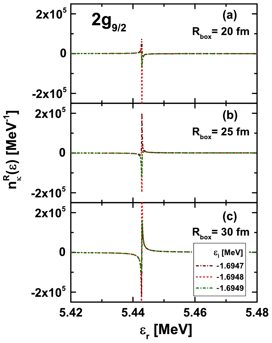
Figure 3. (color online) As Fig. 2, but for the single-neutron resonant state
$ 2g_{9/2} $ in$ ^{120} {\rm{Sn}}.$ Another advantage of the GF method for resonant states is that it can also describe the density distributions in the coordinate space. Here, according to Refs. [50–52], we use the density
$ \rho_{\kappa}(r,\varepsilon) $ defined at resonance energy$ \varepsilon = E $ to describe the distribution for a resonant state in the coordinate space, which is calculated by$ \begin{array}{*{20}{l}} \rho_{\kappa}(r,\varepsilon) =-\dfrac{(2j+1)}{4\pi r^2}\dfrac{1}{\pi}{{\rm{Im}}}\left[{\cal G}_{\kappa}^{(11)}(r,r;E)+{\cal G}_{\kappa}^{(22)}(r,r;E)\right]. \end{array} $

(17) In Fig. 4, the density distribution
$ \rho_{\kappa}(r,\varepsilon) $ at the resonance energy$ \varepsilon = 0.8705\; $ MeV for the state$ 2f_{5/2} $ in$ ^{120} {\rm{Sn}}$ is shown. The space dependence is also verified by performing calculations in different box sizes$ R_{\mathrm{box}} = 20 $ ,$ 25 $ , and$ 30 $ fm. Exactly the same density distribution in the entire coordinate space is obtained with different space sizes, demonstrating again the advantage of GF method. Further, we observe that the density distribution for the narrow$ 2f_{5/2} $ is highly localized, behaving as a bound state.
Figure 4. (color online) Density distributions
$ \rho_{\kappa}(r,\varepsilon) $ for single-neutron resonant state$ 2f_{5/2} $ at resonant energy$ \varepsilon = 0.8705 $ MeV plotted in coordinate space. Calculations are performed with different space sizes$ R_{\mathrm{box}} = 20$ , 25, and 30 fm.According to the above studies, the GF method is effective and reliable in describing resonant states, no matter whether it is narrow or broad. Resonance energies
$ E-{\rm i}\Gamma/2 $ can be easily obtained by searching for the poles of GF or extremes of DOS. In Fig. 5, we plot all the obtained single-neutron resonant states in$ ^{120} {\rm{Sn}}$ , identified by scanning the complex energy$ \varepsilon $ in a wide range for different$ \kappa $ blocks and searching for resonant states by observing extremes. Compared with the results in our previous study (see Fig. 6 in Ref. [85]) in which the resonant states were identified by comparing the DOSs for nucleons moving in the mean field potentials with those for free particles, new resonant states$ 2g_{7/2} $ ,$ 2g_{9/2} $ ,$ 2h_{11/2} $ , and$ 1j_{13/2} $ with very broad widths ranging from$ 3 $ to$ 13 $ MeV are also observed. In Table 1, we list the energies$ E-{\rm i}\Gamma/2 $ of the single-neutron resonant states obtained by RMF-GF method and compare them with the results in the previous GF calculations [85]. The accuracy is highly improved with the new approach by the GF method, both for the narrow resonant states and broad ones. For example, the uncertainty is well constrained within$ 1.0\times 10^{-8} $ MeV for the extremely narrow resonant state$ h_{9/2} $ . Notably, for the very narrow resonant states, the scanning energy step$ {\rm d}\varepsilon $ for the imaginary part in calculating DOSs$ n(\varepsilon) $ must be much smaller. It is$ 1\times 10^{-8} $ MeV for the resonance$ h_{9/2} $ , and only with such a small imaginary energy step, the reverse of DOSs extremes can be observed.positive parity present study previous study negative parity present work previous work 2g7/2 6.3585−i3.1052 3p1/2 0.0504−i0.0164 0.031−i0.043 2g9/2 5.4428−i1.6948 2f5/2 0.8705−i0.0325 0.887−i0.032 1i11/2 9.8544−i0.6413 9.700−i0.636 1h9/2 0.2508−i4×10−8 0.251−i0.0001 1i13/2 3.4786−i0.0024 3.469−i0.002 2h11/2 10.5130−i6.7681 1j13/2 18.1846−i3.1531 1j15/2 12.8929−i0.5322 12.956−i0.688 Table 1. Energies and widths
$ E-{\rm i}\Gamma/2 $ (in MeV) of single-neutron resonant states$ nl_j $ in$ ^{120} {\rm{Sn}}$ obtained by GF-RMF method with PK1 effective interaction, compared with results of previous GF calculations [85].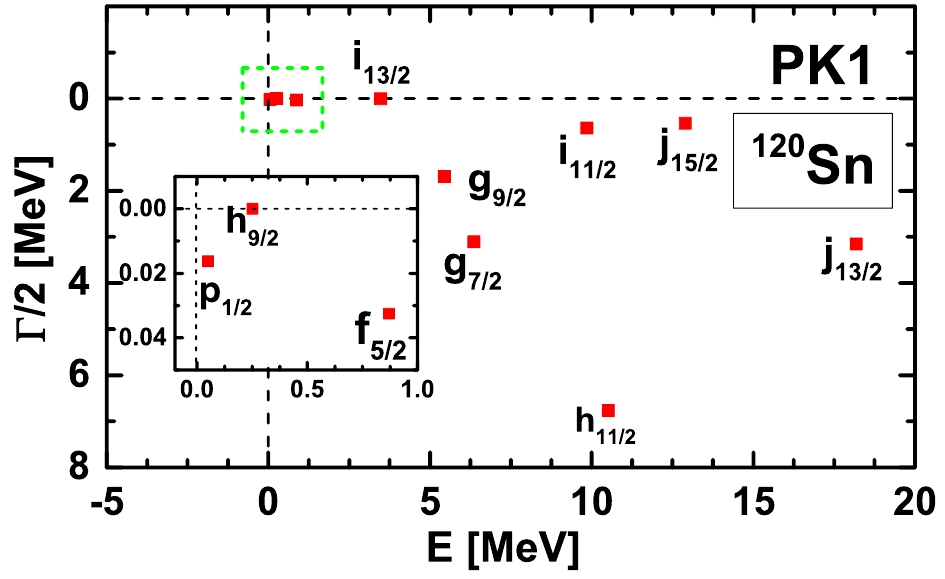
Figure 5. (color online) Single-neutron resonant states in
$ ^{120} {\rm{Sn}}$ obtained by RMF-GF method with PK1 effective interaction.Finally, to compare our results with those obtained with CMR [18], CSM [25], RSM [32], and ACCC [39] methods, we also calculate the resonant states with the RMF-GF method by taking the NL3 [91] effective interaction. The energies
$ E-{\rm i}\Gamma/2 $ for the single-neutron resonant states$ 2f_{5/2} $ ,$ 1i_{11/2} $ ,$ 1i_{13/2} $ , and$ 1j_{15/2} $ by those methods are listed in Table 2. We find that the results by the GF method are all consistent with those of other four methods, particularly the CMR and CSM methods. In fact, according to our previous study for the resonances in deformed nuclei [89], it was found that GF method and CMR can obtain exactly the same energies for most of the resonant states. One possible reason for the slight difference in the present results may come from the mean-field potential obtained in the iteration calculations of RMF theory. Further, the GF and CMR methods are performed very differently. The GF method is worked in the coordinate space, where the resonant states are obtained by searching for its poles corresponding to the eigenvalues of the Dirac equation. However, the CMR method is implemented in the momentum space by diagonalizing the Dirac Hamiltonian.$nl_{j}$ 

GF CMR [18] CSM [25] RSM [32] ACCC [39] $2f_{5/2}$ 

$ 0.674-{\rm i}0.015$ 

$ 0.678-{\rm i}0.015$ 

$ 0.670-{\rm i}0.010$ 

$ 0.674-{\rm i}0.015$ 

$ 0.685-{\rm i}0.012$ 

$1i_{13/2}$ 

$ 3.263-{\rm i}0.002$ 

$ 3.267-{\rm i}0.002$ 

$ 3.266-{\rm i}0.002$ 

$ 3.266-{\rm i}0.002$ 

$ 3.262-{\rm i}0.002$ 

$1i_{11/2}$ 

$ 9.601-{\rm i}0.607$ 

$ 9.607-{\rm i}0.608$ 

$ 9.597-{\rm i}0.606$ 

$ 9.559-{\rm i}0.602$ 

$ 9.600-{\rm i}0.555$ 

$1j_{15/2}$ 

$12.579-{\rm i}0.496$ 

$12.584-{\rm i}0.496$ 

$12.577-{\rm i}0.496$ 

$12.564-{\rm i}0.486$ 

$12.600-{\rm i}0.450$ 

Table 2. Energies and widths
$ E-{\rm i}\Gamma/2 $ (in MeV) of single-neutron resonant states in$ ^{120} {\rm{Sn}}$ obtained by GF method based on RMF theory, in comparison with results by RMF-CMR, RMF-CSM, RMF-RSM, and RMF-ACCC methods. All calculations are performed with NL3 effective interaction. -
Single-particle resonances play crucial roles in the structures of exotic nuclei. Numerous methods such as CMR, CSM, RSM, and ACCC have been proposed to study resonant states. In this work, we applied the Green's function method to study the single-particle resonances based on the RMF theory. Instead of searching for resonant states by comparing the density of states for nucleons in the mean field potentials with those for free particles, a direct and effective approach that searches for the extremes of the density of states or the poles of the GF was implemented for all kinds of resonant states, both narrow and broad.
Taking
$ ^{120} {\rm{Sn}}$ as an example, the resonant states are studied by the RMF-GF method by taking PK1 effective interaction. The obtained energies and widths are highly stable with the change of coordinate space size. The density distributions for resonant states can also be plotted. In comparison with our previous study [85], new resonant states$ 2g_{7/2} $ ,$ 2g_{9/2} $ ,$ 2h_{11/2} $ , and$ 1j_{13/2} $ with broad widths are identified. Furthermore, the accuracy for the very narrow resonant state$ h_{9/2} $ is improved to be$ 1\times 10^{-8} $ MeV. Further, to compare our results with those by CMR, CSM, RSM, and ACCC methods, calculations for$ ^{120} {\rm{Sn}}$ by taking NL3 parameter are also perfromed. It is found that results obtained by the GF method are highly similar to those by CMR and CSM, although the methods differ significantly.
Single-particle resonant states with Green’s function method
- Received Date: 2020-03-16
- Available Online: 2020-08-01
Abstract: This study employs the relativistic mean field theory with the Green's function method to study the single-particle resonant states. In contrast to our previous work [Phys. Rev. C, 90: 054321 (2014)], the resonant states are identified by searching for the poles of Green's function or the extremes of the density of states. This new approach is highly effective for all kinds of resonant states, no matter whether they are broad or narrow. The dependence on the space size for the resonant energies, widths, and the density distributions in the coordinate space has been checked and was found to be very stable. Taking 120Sn as an example, four new broad resonant states


 DownLoad: