


 Abstract
 HTML
HTML Reference
 Related
 PDF
PDF


-
According to the standard model of cosmology, as the universe expands and cools down, the universe undergoes a series of phase transitions, which could lead to the generation of topological defects. In this regard, the quark-hadron phase transition can be considered one of the main evolution steps of the universe, where the quark-gluon is transformed into hadron gas. This phase transition that occurs in the early universe has been studied for more than three decades [1-8]. The phase transition is a specified prediction of quantum chromodynamics (QCD) of the first or second-order. Further, the transition may be a smooth crossover with rapid changes that strongly depend on the values of quark masses. Lattice QCD computation applied to two quark flavors implies that QCD makes a smooth crossover transition [9-11]. Possibly, in early evolution, the relic quark-gluon objects are created due to such a transition.
The quark mass and flavor have a crucial role in determining the order of the phase transition. Ref. [12] was among the first studies to investigate the QHP transition in the expanding universe. As the temperature of the deconfined quark-gluon plasma falls below the critical temperature
$ T_c $ $ \simeq 150\; {\rm{MeV}} $ , it is energetically capable to form color-confined hadrons, which mainly consist of pions, along with a few neutrons and protons, which are a direct result of the conservation of the net baryon number. As a consequence of the first-order phase transition, the hadron phase does not form immediately. To overcome the energy cost of formation of the surface of the bubble and the new hadron phase, supercooling is required. Latent heat is released as the nucleation of the hadron bubble, which leads to appearance of a spherical shocking wave that crosses the surrounding supercooled quark-hadron plasma. This phenomenon warms the plasma up to the critical temperature and precludes any other nucleation in the region by one or more shock fronts. In general, bubble growth is described by deflagrations, with a shock front preceding the actual transition front. As the universe temperature reaches the critical temperature, the nucleation stops. Then, with the cost of the quark phase, the hadron bubbles grow and ultimately percolate or coalesce. By transforming all quark-gluon phase to hadron, the transition ceases, of course, the possible quark nugget production has been ignored in this study [13-25].The general theory of relativity, which provides a geometrical description of spacetime, is one of the most successful theories that passed numerous experimental tests and is in good agreement with the observational data. Other alternative theories of gravity exist beside the general theory of relativity. The scalar-tensor theory is among these theories, introduced by P. Jordan, where a four-dimensional curved manifold is embedded in five-dimensional flat spacetime [26]. Among all types of scalar-tensor theories (STT), the Brans-Dicke (BD) theory is the most popular one [27]. BD theory, which is based on the idea of Mach, has a non-minimal coupling to gravity. The theory has significant potential to solve some cosmological problems [28-35]. Furthermore, the BD formalism of gravity also demonstrates its abilities during the chain inflation, which could facilitate nucleation between different vacua. Ref. [36] showed that one of the solutions of overcoming the problem of a slow nucleation rate in chain inflation is to extend the gravity sector of the model to the BD theory of gravity.
Another alternative is higher-dimensional theories, which have a long history. The starting point of these theories could be attributed to the theory of Kaluza-Klein, which a classic unified theory of electromagnetism and gravitation by utilizing the concept of the fifth dimension. In 1999, inspired by M-theory, Randall and Sundrum presented a novel special case of the brane world scenario [37], where the standard matter and its interaction are confined to a four-dimensional hypersurface (the brane) embedded in five-dimensional spacetime (the bulk). The extra dimension in RS brane gravity does not need to be compact. The dynamical equation governing the evolution of the brane has some modified terms in comparison to the standard cosmology, such as the appearance of the quadratic term of brane energy density. However, at low energy densities, the evolution equations could come back to the standard one [38-45]. Another model of the brane-world was introduced by Dvali, Gabadadze, and Porrati (DGP) [46] in 2000. The main difference between this model and the RS-brane-world is the presence of an Einstein term in brane action as well as the bulk action. Because the matter confined on brane is coupled with bulk gravity, several quantum corrections are induced on brane action. The curvature scalar in brane action is the result of such a correction. The DGP model contains two branches related to two values of the
$ \epsilon $ parameter, which appears in the Friedmann equation of the model, as$ \epsilon = -1 $ (normal branch) and$ \epsilon = 1 $ (self-accelerating branch). The self-accelerating branch seems to have a ghost-instability problem; however, this instability occurs at the quantum level, where the theory of gravity is unclear as well. Therefore, numerous cosmologists believe that leaving the self-accelerating branch because of its ghost-instability problem might be a rash decision, with numerous studies on various topics of this branch [47-51].The DGP model is highly successful in the investigation of the late time evolution of the Universe. Therefore, we consider this framework for the early times evolution of the Universe. The main purpose of this study is to consider the QHP transition in the DGP model of gravity including an STT in brane action instead of the usual Einstein-Hilbert action by supposing that the phase transition is described by both the first-order phase transition and crossover scenarios. As mentioned before, the BD theory is an interesting alternative theory of gravity, which overcomes some problems of general relativity in standard four-dimension cosmology. The evolution equation in this model comes in a different form with standard cosmology, and a different result is expected.
This paper is structured as follows: In Sec. 2, we derive the basic equations of the model. In Sec. 3, the first-order phase transition is briefly explained. Subsequently, we investigate this type of phase transition in our model. The QHP transition is considered by assuming the smooth crossover approach in Sec. 4, where the evolution of the temperature for both the high and low-temperature regime is explored. The results are summarized in Sec. 5, and a comparison is made with the results obtained in previous studies.
-
In the brane-world scenario, we take a four-dimensional spacetime (the brane) as the Universe, which was embedded in five-dimensional spacetime (the bulk). We consider the DGP model of the brane world scenario with the following action
$ \begin{split} {\cal{S}} =& S_{\rm bulk} + S_{\rm brane} \\ =& \int {\rm d}^5x \sqrt{-{\cal{G}}} \left( {{\cal{R}} \over 2\kappa_5^2} - \Lambda \right) \\ & + \int {\rm d}^4x\sqrt{-g}\left( [\tilde{K}] + {1 \over 2} \Big[ \phi R-{\omega\over{\phi}}\phi^{,\alpha}\phi_{,\alpha} \Big] +{\cal{L}}_m \right), \end{split} $

(1) where
$ \tilde{K} = {[K] /\kappa_5^2} $ , and$ [K] $ is the exterior curvature. The action is presented in terms of five-dimensional coordinates$ (x^0, x^1, x^2, x^3, y) $ on bulk, where the hypersurface$ y = 0 $ describes the brane. In the bulk action,$ {\cal{G}} $ is the determinant of the five-dimensional metric$ {\cal{G}}_{AB} $ with signature$ (- + + + +) $ ,$ {\cal{R}} $ is five-dimensional Ricci scalar constructed from$ {\cal{G}}_{AB} $ ,$ \Lambda $ is five-dimensional cosmological constant, and$ \kappa_5 $ is a redefinition of five dimensional Newtonian gravitational constant$ G_5 $ as$ \kappa_5^2 = 8\pi G_5 $ , which is related to five dimensional Plank mass by$ \kappa_5^2 = M_5^{-3} $ . In the brane action,$ g $ and$ R $ are determinants of four-dimensional induced metric and Ricci scalar related to induced metric$ g_{\mu\nu} = \delta^A_{\ \mu} \delta^B_{\ \nu} {\cal{G}}_{AB} $ , respectively. The BD scalar field is denoted by$ \phi $ , which lives on the brane without a potential term, and$ \omega $ is a dimensionless coupling constant, which determines the coupling between the gravity and$ \phi $ . The Lagrangian term$ {\cal{L}}_m $ in the brane action includes the Lagrangian of the brane-matter, denoted by$ L_m $ , and the brane tension,$ \lambda $ . Thus,$ {\cal{L}}_m = L_m - \lambda $ .The Einstein field equation is derived by defining the variation of action with respect to the metric as
$ ^{(5)}G_{AB} = {\cal{R}}_{AB} - {\cal{G}}_{AB}{\cal{R}} = \kappa_5^2 \left[ T^{(\Lambda)}_{AB} + T_{AB}\delta(y) \right]. $

(2) Further, the energy-momentum tensor of the bulk cosmological constant is described by
$ T^{(\Lambda)}_{AB} = -\Lambda {\cal{G}}_{AB} $ , and$ T_{AB} $ is the total brane energy-momentum tensor with the following definition$ T_{AB} \;\; = \;\; g_A^{\ \ \mu}g_B^{\ \ \nu} \Big[ \phi T^{G}_{\mu\nu} + T^{(\phi)}_{\mu\nu} + T^{(m)}_{\mu\nu} \Big], $

(3) where
$ T^G_{\mu\nu} $ denotes the presence of a curvature scalar in brane action and behaves as a source of gravity.$ T^{(\phi)}_{\mu\nu} $ is related to the BD scalar field, and$ T^{(m)}_{\mu\nu} $ is related to the brane-matter energy-momentum tensor. The matter section of brane is assumed to be filled with the perfect fluid$ T^{(m)\mu}_{\ \ \ \nu} = \delta(y) {\rm{diag}}(-\rho_b, p_b, p_b, p_b, 0) $ , where$ \rho_b = \rho + \lambda $ is the brane-matter energy density, and$ p_b = p-\lambda $ is the brane-matter pressure.Because brane matter has no direct coupling to the other component in the action, the continuity of brane matter is preserved, i.e.,
$ \dot\rho + 3H(\rho+p) = 0. $

(4) In contrast, the equation of motion of BD scalar field
$ \phi $ is obtained by taking the variation of action with respect to the scalar field as$ {2\omega \over \phi}- \triangle \phi - {\omega \over \phi^2} \partial_\alpha \phi \partial^\alpha \phi + R = 0 . $

(5) According to [38-40,52,53], the Friedmann equation of the model can be derived after some algebraic analysis as
$ H^2 = {\Lambda \over 6 M_5^3} + \frac{1}{36 M_5^6} \Bigg[ 3A\phi H^2 + (\rho+\lambda) \Bigg]^2 + {\zeta \over a^4}, $

(6) where
$ A = {\beta^2\omega / 6} -(1 +\beta) $ ; notably, in obtaining above equation, it is assumed that$ \phi = \phi_0 a^\beta $ [54,55]. The effective DGP length scale in this model is defined as$l_{\rm effDGP} = {|A|\phi / M_5^3}$ , where$ \phi $ is a function of time, such that the effective DGP length scale is varying in time. A constant DGP length scale is introduced as$ l_c = {|A| \phi_0 / M_5^3} $ . Then, the familiar form of the Friedmann equation is given by$ H^2 = {2 \over \Phi^2} \left(\chi + \epsilon \sqrt{ \chi^2 - \Phi^2 \left[ \Lambda_4 + {\rho_b^2 - \lambda^2 \over 36 M_5^6} \right]}\right), $

(7) where
$ \chi = \big[1- (\Phi \rho_b) / 6 M_5^3 \big] $ ,$ \Phi = A \phi / M_5^3 = A \Phi_0 a^\beta $ (with$ \Phi_0 \equiv \phi_0 / M_5^3 $ ), and$ \epsilon = \pm 1 $ . Further, the brane effective cosmological constant is described by$ \Lambda_4 = \big[\Lambda + $ $ ( \lambda^2 / 6 M_5^3) \big] / 6 M_5^3 $ , which as the RS-model was assumed to be zero. The last term that describes the dark radiation has been ignored as well. According to [56,57], for convenience, the five-dimensional Planck mass is set to one, i.e.,$ \kappa_5 = 1 $ , for the remainder of the paper. -
The phase transition in the temperature interval
$ 180\;{\rm{MeV}} < T < 250\;{\rm{MeV}} $ is characterized by sigular behavior of the partition function, which might be a first or second order phase transition [24]. The phase transition at higher or lower temperature occurs through trace anomaly or hadronic resonance gas, which will be investigated in the following section. In this section, we assumed that the quark-hadron phase transition is first order, which happens in the aforementioned temperature interval (refer to [58] and references therein for more information on the first order quark-hadron phase transition). According to [24], the matter equation of state in the quark-gluon phase is expressed as$ \rho _q = 3a_q T^4 +W(T), \qquad p_q = a_q T^4 -W(T), $

(8) where the subscript
$ q $ denotes the quark-gluon matter, and the constant$ a_q $ is equal to$ a_q = 61.75(\pi^2/90) $ .$ W(T) $ , denoting the potential energy density, is given by [24],$ W(T) = B+\gamma_T T^2 - \alpha_{T} T^{4}, $

(9) where the constant
$ B $ is the bag pressure constant,$ \alpha_T = 7\pi^2/20 $ ,$ \gamma_T = m^2_s/4 $ , where the mass of the strange quark,$ m_s $ , is in the range (60 – 200) MeV. This type of potential$ W $ can be found out in the model where the quark fields interact with a chiral formed from a scalar field and the$ \pi $ meson field [59]. The constant$ B^{1/4} $ in the above equation could be determined through the results obtained from low energy hadron spectroscopy, heavy ion collisions, and from phenomenological fits of light hadron properties stating that it must be between 100 and 200 MeV [58].The cosmological fluid, which is commonly assumed to be an ideal gas, can be described by the Maxwell-Boltzmann distribution function with energy density
$ \rho_h $ and pressure$ p_h $ , obeying the following equation of state$ p_h = {1 \over 3} \rho_h = a_\pi T^{4} , $

(10) where the constant is read as
$ a_\pi = 17.25 \pi^2 / 90 $ . In contrast, it has been shown that the identity$ p_q(T_c) = p_h(T_c) $ defines a critical temperature$ T_c $ [60-64] in which for the present model, one has$ T_c = {\Bigg[{\frac{\gamma_T + \sqrt{\gamma^2_T+ 4B(a_q+\alpha_T-a_{\pi})}}{2(a_q+\alpha_T -a_{\pi})}}\Bigg]}^{1/ 2}\approx 125\; {\rm{MeV}}. $

(11) where in obtaining the above result, it is assumed that
$ m_s = B^{1/4} = 200\; {\rm{MeV}} $ .Because this phase transition is of first order, discontinuities in the energy density, number density, and entropy are found when they cross the critical curve. This behavior of the quantities is perfectly described in Ref. [13]. The main quantities that deal with them in the present study are the energy density, pressure, scale factor, and the temperature, which are determined through the conservation equation, Friedmann equation, and equation of state. In the subsequent subsections, the behavior of these quantities will be studied in the framework of DGP brane-world, including a BD scalar field in the brane before, during, and after the phase transition.
-
At the temperature higher than the critical temperature
$ T > T_c $ , i.e., before the phase transition, matter is in the quark phase, which is described by the equation of state Eq. (8). The Hubble parameter is determined by applying the equation of state Eq. (8) on the conservation equation (4), as$ H = - \bigg[ {3a_q-\alpha_T \over 3a_q} + {\gamma_T \over 6a_qT^2}\bigg] {\dot{T} \over T} , $

(12) where the potential energy density (9) is utilized. By integrating the above equation, the scale factor of the universe in this phase can be extracted as
$ a(T) = c T^{\textstyle{\alpha_T - 3a_q \over 3a_q}} \exp\left( {\gamma_T \over 12a_q T^2} \right). $

(13) Finally, the evolution of the temperature is obtained by substituting the above results in the Friedmann equation (7), which reads as
$ \begin{split} \dot{T} =& - {6a_qT^3 \over 2(3a_q - \alpha_T)T^2 + \gamma_T} \\ &\times \Bigg[ {2 \over \Phi^2} \left(\chi + \epsilon \sqrt{ \chi^2 - {\Phi^2 \over 36} (\rho_b^2 - \lambda^2)}\right)\Bigg]^{1/2} . \end{split} $

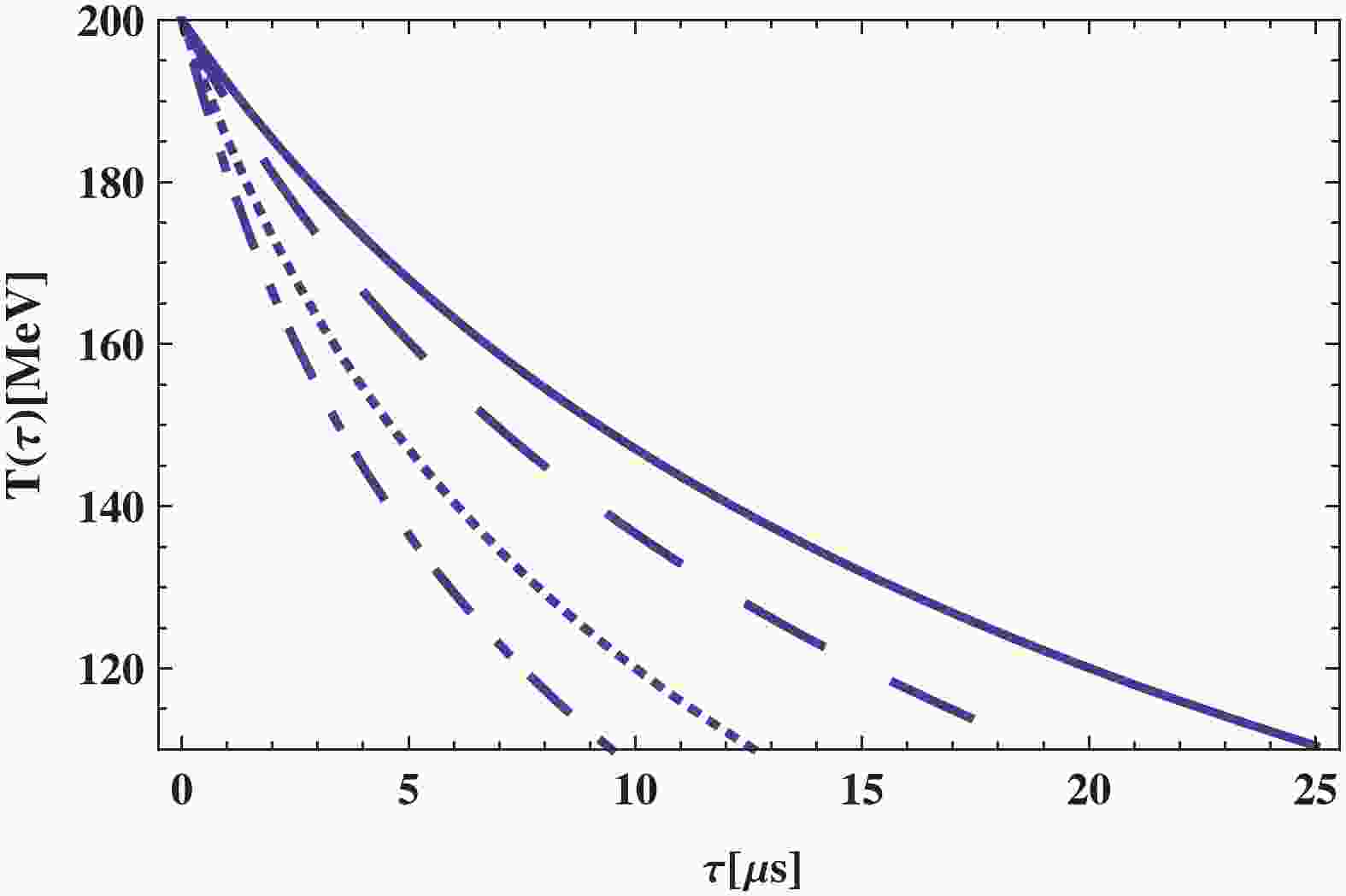
(14) This equation describes the behavior of the temperature in terms of the cosmic time. The numerical result obtained for the temperature is depicted in Figs. 1 and 2, respectively for the normal branch (
$ \epsilon = -1 $ ) and self-accelerating branch ($ \epsilon = +1 $ ). The temperature in the quark phase decreases with time, where the increasing of the BD coupling$ \omega $ results in the reduction of temperature. Further, for the self-accelerating branch of the model, the temperature reaches the critical temperature faster than the normal branch.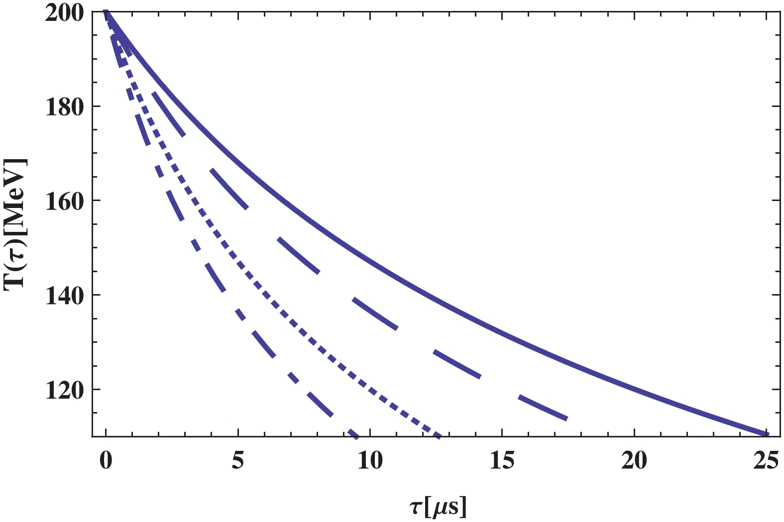
Figure 1. (color online)
${\bf{\underline{\epsilon = -1}}}$ :$T$ versus$\tau$ in quark-gluon phase plotted for different values of BD coupling constant$\omega$ as:$\omega = 2.1 \times 10^{3}$ (solid line),$\omega = 2.3 \times 10^{3}$ (dashed line),$\omega = 2.5 \times 10^{3}$ (dotted line),$\omega = 2.7 \times 10^{3}$ (dotted-dashed line). Other constant parameters are:$\beta = 5.24 \times 10^{-2}$ ,$\Phi_0 = 2 \times 10^4\; {{\rm{MeV}}^{-1}}$ ,$\lambda = 10^{9} \;{{\rm{MeV}}^4}$ , and$B^{1/4} = 200 \;{\rm{MeV}}$ .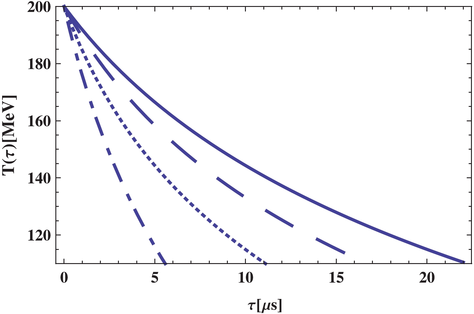
Figure 2. (color online)
${\bf{\underline{\epsilon = +1}}}$ :$T$ versus$\tau$ in quark-gluon phase plotted for different values of BD coupling constant$\omega$ as:$\omega = 2.1 \times 10^{3}$ (solid line),$\omega = 2.3 \times 10^{3}$ (dashed line),$\omega = 2.5 \times 10^{3}$ (dotted line),$\omega = 2.7 \times 10^{3}$ (dotted-dashed line). Other constant parameters are:$\beta = 5.24 \times 10^{-2}$ ,$\Phi_0 = 2 \times 10^4\;{{\rm{MeV}}^{-1}}$ ,$\lambda = 10^{9}\;{{\rm{MeV}}^4}$ , and$B^{1/4} = 200\; {\rm{MeV}}$ . -
Ignoring the temperature effect results in a constant potential
$ W(T) = B $ , which is another interesting model that deals with quark confinement and is worth considering. This is related to an elastic bag model, which allows the quarks to freely move around. Because of this constant potential, the equation of state obtains a simple form$ p_q = {(\rho_q -4B) / 3} $ , leading to the following Hubble parameter and scale factor$ H = - {\dot{T} \over T} ; \qquad a(T) = {c \over T}. $

(15) Applying above result Eq. (15) in the Friedmann equation, leads to the temperature evolution equation given by
$ \dot{T} = - T \Bigg[ {2 \over \Phi^2} \left(\chi + \epsilon \sqrt{ \chi^2 - {\Phi^2 \over 36} (\rho_b^2 - \lambda^2)}\right)\Bigg]^{1/2} . $

(16) The equation yields the behavior of the temperature in terms of the cosmic time. Solving the above differential equation numerically, the result is plotted in Figs. 3 and 4 for normal and self-accelerating branches ,respectively, for different choices of the BD coupling
$ \omega $ , where one could find that the enhancement of BD constant results in lower temperature. In general, the temperature decreases with time, and this happens faster for a self-accelerating branch than for the normal branch.
Figure 3. (color online)
${\bf{\underline{\epsilon = -1}}}$ : Temperature$T$ , as a function of time,$t$ , in quark-gluon phase plotted for constant self-interacting potential$W(T) = B$ , and for different values of BD coupling constant$\omega$ as:$\omega = 2.1 \times 10^{3}$ (solid line),$\omega = 2.3 \times 10^{3}$ (dashed line),$\omega = 2.5 \times 10^{3}$ (dotted line),$\omega = 2.7 \times 10^{3}$ (dotted-dashed line). Other constant parameters are taken as:$\beta = 5.24 \times 10^{-2}$ ,$\Phi_0 = 2 \times 10^4\;{{\rm{MeV}}^{-1}}$ ,$\lambda = 10^{9}\;{{\rm{MeV}}^4}$ , and$B^{1/4} = 200\;{\rm{MeV}}$ .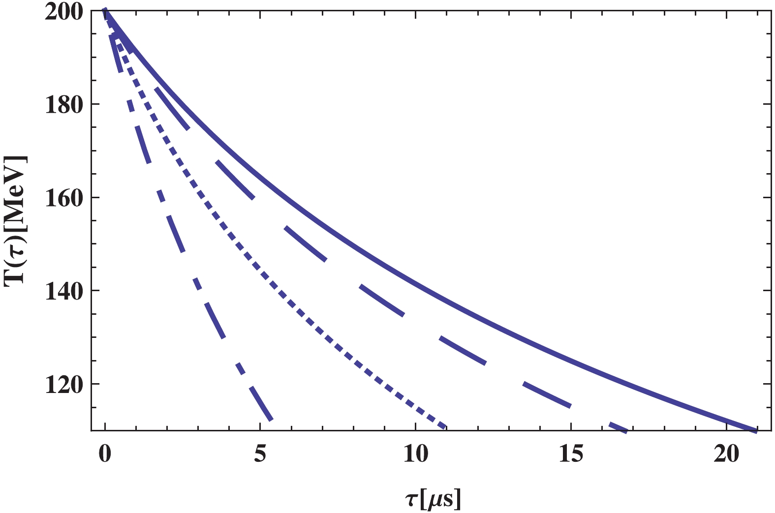
Figure 4. (color online)
${\bf{\underline{\epsilon = +1}}}$ : Temperature$T$ , as a function of time,$t$ , in quark-gluon phase plotted for constant self-interacting potential$W(T) = B$ , and for different values of BD coupling constant$\omega$ as:$\omega = 2.1 \times 10^{3}$ (solid line),$\omega = 2.3 \times 10^{3}$ (dashed line),$\omega = 2.5 \times 10^{3}$ (dotted line),$\omega = 2.7 \times 10^{3}$ (dotted-dashed line). Other constant parameters are taken as:$\beta = 5.24 \times 10^{-2}$ ,$\Phi_0 = 2 \times 10^4\;{{\rm{MeV}}^{-1}}$ ,$\lambda = 10^{9}\;{{\rm{MeV}}^4}$ , and$B^{1/4} = 200\;{\rm{MeV}}$ . -
During the phase transition, the matter density changes from the quark density
$ \rho_Q $ to the hadron energy density$ \rho_H $ , which are respectively$ \rho_Q = 5 \times 10^9 \;{\rm{MeV}}^4 $ and$ \rho_H \approx 1.38 \times 10^9 \;{\rm{MeV}}^4 $ (notably,$ \rho_Q $ stands for the energy density of the universe when it is in the pure quark phase, namely when all matter of the universe is quarks. Similarly,$ \rho_H $ stands for the energy density of the universe when it is in the pure hadron phase). In this phase transition, the temperature, pressure, entropy, and enthalpy remain constant at$ T_c = 125\;{\rm{MeV}} $ and constant pressure$ p_c \approx 4.6 \times 10^8\;{\rm{MeV}}^4 $ .The universe transitions from a pure quark phase to a pure hadron phase. Mid-transition, the energy density of the universe is a composite of quarks and hadrons. Then, the energy density can be expressed in terms of a volume fraction term in the hadron phase, which is defined as [56,57,58,65,66]
$ \rho = \rho_H h(t) + [1-h(t)]\rho_{Q}. $

(17) At the beginning of the transition (
$ h(t) = 0 $ ), all matter is in the phase of the quark, and by passing time the matter phase changes to the hadron phase, where at the end of the transition ($ h(t) = 1 $ ) all matter is in the hadron phase. Imposing Eq. (17) on the conservation equation leads to the following Hubble parameter$ H = -{1 \over 3} {(\rho_H - \rho_Q)\dot{h} \over \rho_Q+p_c+(\rho_H-\rho_Q)h} = -{1 \over 3} {r\dot{h} \over 1+rh}, $

(18) where the parameter
$ r $ is defined as$ r = (\rho_H - \rho_Q) / (\rho_Q+p_c) $ . The scale factor is obtained by taking an integral from the above relation as$ a(t) = a_0 \big[ 1+rh \big]^{-1/3}. $

(19) Figure 5 illustrates the scale factor of the universe versus the volume fraction during the quark hadron phase transition, which expresses an expansion for the universe in the era where the temperature, pressure, entropy, and enthalpy are constant.
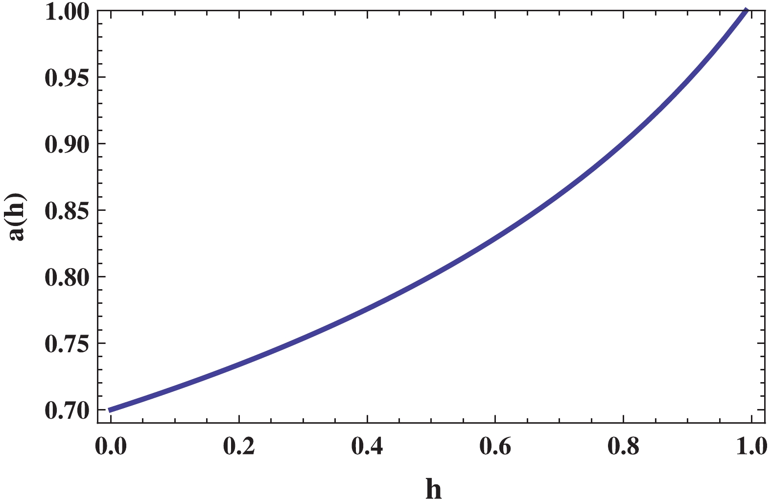
Figure 5. (color online) Scale factor as a function of hadron volume fraction during QHPT in DGP brane gravity with BD scalar field in brane.
By Utilizing the Hubble parameter (18) in the Friedmann equation (7), one could find the evolution equation of the volume fraction as
$ \begin{split} \dot{h} = - {3(1+rh) \over r} \Bigg[ {2 \over \Phi^2} \left(\chi + \epsilon \sqrt{ \chi^2 - {\Phi^2 \over 36} (\rho_b^2 - \lambda^2)}\right) \Bigg]^{1/2}. \end{split} $

(20) By finding the numerical solution for the above differential equation, the behavior of the volume fraction in terms of the cosmic time during the phase transition is presented in Figs. 6 and 7 for different choices of the BD coupling
$ \omega $ for both branches. More BD coupling results in a faster phase transition. Further, for the self-accelerating branch, the transition occurs earlier, and the universe enters the pure hadron phase faster than the normal branch.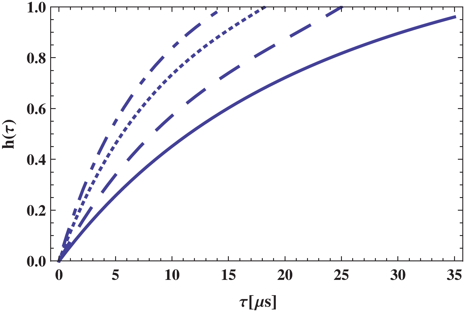
Figure 6. (color online)
${\bf{\underline{\epsilon = -1}}}$ : Hadron volume fraction as a function of cosmic time$\tau$ has been depicted for different values of BD coupling constant$\omega$ as:$\omega = 2.1 \times 10^{3}$ (solid line),$\omega = 2.3 \times 10^{3}$ (dashed line),$\omega = 2.5 \times 10^{3}$ (dotted line),$\omega = 2.7 \times 10^{3}$ (dotted-dashed line). Other constant parameters are:$\beta = 5.24 \times 10^{-2}$ ,$\Phi_0 = 2 \times 10^4\;{{\rm{MeV}}^{-1}}$ ,$\lambda = 10^{9}\;{{\rm{MeV}}^4}$ , and$B^{1/4} = 200\;{\rm{MeV}}$ .
Figure 7. (color online)
${\bf{\underline{\epsilon = +1}}}$ : Hadron volume fraction as a function of cosmic time$\tau$ has been depicted for different values of BD coupling constant$\omega$ as:$\omega = 2.1 \times 10^{3}$ (solid line),$\omega = 2.3 \times 10^{3}$ (dashed line),$\omega = 2.5 \times 10^{3}$ (dotted line),$\omega = 2.7 \times 10^{3}$ (dotted-dashed line). Other constant parameters are:$\beta = 5.24 \times 10^{-2}$ ,$\Phi_0 = 2 \times 10^4\;{{\rm{MeV}}^{-1}}$ ,$\lambda = 10^{9}\;{{\rm{MeV}}^4}$ , and$B^{1/4} = 200\;{\rm{MeV}}$ . -
After the phase transition, the universe is in the pure hadronic phase, where the following simple equation describes the equation of state of the matter
$ \rho_h = 3p_h = 3a_\pi T^{4}. $

(21) Then, following the same processes, the Hubble parameter and the scale factor are easily derived as
$ H = -{\dot{T} \over T} ; \qquad a(T) = c {T_c \over T}. $

(22) Inserting the above equation into the Firedmann equation results in a evolution equation for the temperature in the pure hadronic phase of the universe
$ \dot{T} = - T \Bigg[ {2 \over \Phi^2} \left(\chi + \epsilon \sqrt{ \chi^2 - {\Phi^2 \over 36} (\rho_b^2 - \lambda^2)}\right)\Bigg]^{1/2}. $

(23) Solving the above differential equation numerically, the behavior of the temperature in terms of the cosmic time can be depicted as Figs. 8 and 9, respectively, for the normal and self-accelerating branches for different values of the BD coupling constant
$ \omega $ . The temperature clearly decreases with time, and the hadron phase era of the universe occurs earlier in the self-accelerating branches. Further, for larger values of$ \omega $ , there is lower temperature and the phase transition happens earlier. This result is in good consistency with the previous results regarding the other eras.
Figure 8. (color online)
${\bf{\underline{\epsilon = -1}}}$ : Evolution of temperature$T$ versus$t$ in pure hadronic phase era depicted for different values of BD coupling constant$\omega$ as:$\omega = 2.1 \times 10^{3}$ (solid line),$\omega = 2.3 \times 10^{3}$ (dashed line),$\omega = 2.5 \times 10^{3}$ (dotted line),$\omega = 2.7 \times 10^{3}$ (dotted-dashed line). Other constant parameters are taken as:$\beta = 5.24 \times 10^{-2}$ ,$\Phi_0 = 2 \times 10^4\;{{\rm{MeV}}^{-1}}$ , and$\lambda = 7 \times 10^{10}\;{{\rm{MeV}}^4}$ .
Figure 9. (color online)
${\bf{\underline{\epsilon = +1}}}$ : Evolution of temperature$T$ versus$t$ in pure hadronic phase era depicted for different values of BD coupling constant$\omega$ as:$\omega = 2.1 \times 10^{3}$ (solid line),$\omega = 2.3 \times 10^{3}$ (dashed line),$\omega = 2.5 \times 10^{3}$ (dotted line),$\omega = 2.7 \times 10^{3}$ (dotted-dashed line). Other constant parameters are:$\beta = 5.24 \times 10^{-2}$ ,$\Phi_0 = 2 \times 10^4\;{{\rm{MeV}}^{-1}}$ , and$\lambda = 7 \times 10^{10}\;{{\rm{MeV}}^4}$ . -
In this section, we investigate the lattice QCD phase transition and consider the physical quantities related to the QHP transition in the context of the DGP brane-world scenario with the brane BD scalar field. A brief review on lattice QCD is presented in the following lines. One of the basic phenomena in particle physics is the lattice QCD phase transition, which is involved in any study related to the early time evolution of the universe. According to this scenario, there is a soup of quarks and gluons that interact. Then, hadrons are formed through a crossover transition. Various methods were employed to acquire the equation of state. Studying the nonperturbative regime of the QCD equation of state is possible via the newly presented approach as lattice QCD. In the recent calculation, the equation of state was estimated for the 2+1 flavor QCD. The most extensive estimation of equation of state was performed with the fermion formulation on the lattice with temporal extent
$ N_t = 4, 6 $ [67-69],$ N_t = 8 $ [70] and$ N_t = 6, 8, 10 $ [71]. For the high temperature region$ T > 250\;{\rm{MeV}} $ , one could accurately compute the trace anomaly. Then, in the high temperature regime, the lattice QCD data for the trace anomaly can be utilized to construct a realistic equation of state.For the low temperature regime
$ T < 180\;{\rm{MeV}} $ , the situation is different. In this regime, the trace anomaly is affected by large discretization effect. However, the hadronic resonance gas (HRG) model is a an appropriate approach to construct an equation of state, which has been studied in [72]. -
In the temperature regime
$ T > 250\;{\rm{MeV}} $ , the gluon and quarks are effectively massless and behave like radiation. Applying the trace anomaly to obtain an equation of state determines that the data are fit on a simple form of equation of state as$ \rho(T) \simeq \alpha T^4, \qquad p(T) \simeq \sigma T^4 , $

(24) where the constants
$ \alpha $ and$ \beta $ are found using a least-squares fit as$ \alpha = 14.9702 \pm 009997 $ and$ \sigma = 4.99115 \pm 004474 $ [68,69]. Substituting Eq. (24) into the conservation equation leads to following result, which expresses the scale factor in terms of the temperature as$ a(T) = cT^{\textstyle -\frac{4\alpha}{3(\alpha+\sigma)}}, $

(25) where
$ c $ is a constant of integration. Substituting Eq. (25) into Eq. (7), the temporal evolution of temperature in this regime is derived as$ \dot{T} = - {3(\alpha+\sigma)T \over 4\alpha} \left[ {2 \over \Phi^2} \left(\chi + \epsilon \sqrt{ \chi^2 - {\Phi^2 \over 36} (\rho_b^2 - \lambda^2)}\right) \right]^{1/2}. $

(26) which describes the behavior of temperature as a function of time. The numerical results for the above differential equation were depicted in Fig. 10 for two branches.

Figure 10. (color online) Temperature
$T$ versus cosmic time$\tau$ in high temperature region by smooth crossover procedure in DGP brane gravity with BD scalar field on brane for$ 250\;{\rm{MeV}} \leqslant T \leqslant 700\;{\rm{MeV}}$ . Constant parameters are:$\beta = 2.47 \times 10^{-3}$ ,$\Phi_0 = 2 \times 10^{5}\;{{\rm{MeV}}^{-1}}$ ,$\omega = 10^4$ , and$\lambda = 10^{9}\;{{\rm{MeV}}^4}$ .We plot the numerical results of Eq. (26) in Fig. 10 for two branches. The plots display the effective temperature in the QGP in the BD model of the DGP brane world for the temperature interval
$ 250\;{\rm{MeV}} \leqslant T \leqslant 700\;{\rm{MeV}} $ , acquired with the smooth crossover approach. With time, the universe becomes cooler, and the situation is almost the same for both cases. The higher and lower curves indicate the temperature behavior for the initial temperatures$ 700\;{\rm{MeV}} $ and$ 250\;{\rm{MeV}} $ , respectively. The curve for any other initial value between these two temperatures is in the shaded region. -
Although the trace anomaly is a suitable approach to acquire a realistic equation of state in the high temperature regime, the approach seems to fail in the low temperature regime mostly due to the discretization effect. In the low temperature regime, where
$ T < 180\;{\rm{MeV}} $ , one can achieve an equation of state by the HRG model [72]. In the HRG model, the confinement of QCD is treated as a non-interacting gas of fermions and bosons [73,74]. In this case, the era before the phase transition (namely quark-gluon phase) is considered at low temperature. Then, the Universe is in confinement phase and can be treated as a non-interacting gas of fermions and bosons. The concept of the HRG model is to implicitly account for the strong interaction in the confinement phase by looking at the hadronic resonances only, as these are basically the only relevant degrees of freedom in that phase. It has been shown that the HRG results can be parametrized for the trace anomaly as [72]:$ {I(T) \over T^4}\equiv {\rho -3p \over T^4} = a_1T + a_2T^3 + a_3T^4 + a_4T^{10}, $

(27) where
$ a_1 $ = 4.654 GeV−1,$ a_2 $ =−79 GeV-3,$ a_3 $ = 8081 GeV-4,$ a_4 $ =−7039000 GeV−10, and$ I(T) = \rho(T) - 3p(T) $ is the trace anomally. Through the calculation of the trace anomally$ I(T) $ in the lattice QCD, the energy density, pressure, and entropy could be estimated by using usual thermodynamics identities. The integral of the trace anomaly displays the pressure difference between the temperatures$ T $ and$ T_{\rm{low}} $ $ {p(T) \over T^4 } - {p(T_{\rm{low}})\over T^4_{\rm{low}}} = \int^T_{T_{\rm{low}}} {{\rm d}T' \over T'^5}I(T'). $

(28) The second term on the left hand side of above equation,
$ p \left( T_{\rm{low}}\right) $ , can be ignored for sufficiently small values of the lower integration limit because of exponential suppression [75]. The energy density, which is expressed as$ \rho(T) = I(T) + 3p(T) $ , can be calculated. At the end, using Eqs. (27) and (28), we have the following respective relations for the energy density and pressure:$ \rho(T) \;\; = \;\; 3\eta T^4 + 4a_1 T^5 + 2a_2 T^7 + {7a_3 \over 4}T^8 + {13a_4 \over 10} T^{14}, $

(29) $ p(T) \;\; = \;\; \eta T^4 + a_1 T^5 + {a_2 \over 3} T^7 + {a_3 \over 4}T^8 + {a_4 \over 10} T^{14}, $

(30) where
$ \eta = -0.112 $ .Inserting Eqs. (29) and (30) in the conservation equation, the Hubble parameter can be derived in terms of temperature of its time derivative as
$ H = - {12\eta T^3 + 20a_1T^4 + A(T) \over 3\big[ 4\eta T^4 + 5a_1T^3 + B(T) \big]} \dot{T}, $

(31) where the parameters
$ A(T) $ and$ B(T) $ are defined by$\begin{array}{l} A(T) \;\; = \;\; 14 a_{2}T^{6} + 14 a_{3}T^{7} + \dfrac{91}{5}a_{4} T^{13}, \\ B(T) \;\; = \;\; \dfrac{7}{3} a_{2} T^{7} + 2a_{3} T^{8} + \dfrac{7}{5}a_{4}T^{14}. \end{array} $

To obtain the scale factor as a function of temperature, we must integrate Eq. (31), which results in the following expression
$ a(T) = {c \over T\big[ 60 \eta + 75a_1T + 35a_2 T^3 + 30a_3 T^4 + 21 T^{10} \big]^{1/3}}, $

(32) where
$ c $ is the constant of integration. Finally, using Eq. (31) and the Friedmann equation (7), we can determine the time evolution of temperature$ \begin{split} \dot{T} = & - {3\big[ 4\eta T^4 + 5a_1T^3 + B(T) \big]\over 12\eta T^3 + 20a_1T^4 + A(T)} \\ & \times \left[ {2 \over \Phi^2} \left(\chi + \epsilon \sqrt{ \chi^2 - {\Phi^2 \over 36} (\rho_b^2 - \lambda^2)}\right)\right]^{1/2}. \end{split} $

(33) Differential Eq. (33) describes the behavior of temperature as a function of cosmic time in the QGP for the DGP brane-world scenario with a BD scalar field on the brane for the temperature interval
$ 80\;{\rm{MeV}} \leqslant T \leqslant 180\;{\rm{MeV}} $ . The relation displays the era before the phase transition at low temperature, where the Universe is treated as a non-interacting gas of fermions and bosons, as it is in confinement phase. The equation can be solved numerically, where the obtained results were plotted in Fig. 11 for two branches of the model. The figure illustrates the behavior of temperature in terms of cosmic time. The higher and lower curves display the temperature behavior for the initial values of$ 180\;{\rm{MeV}} $ and$ 80\;{\rm{MeV}} $ , respectively. Further, the corresponding curve for any other initial value in this temperature interval is in the shaded region. The phase transition for the normal branch evidently occurs after the self-accelerating branch.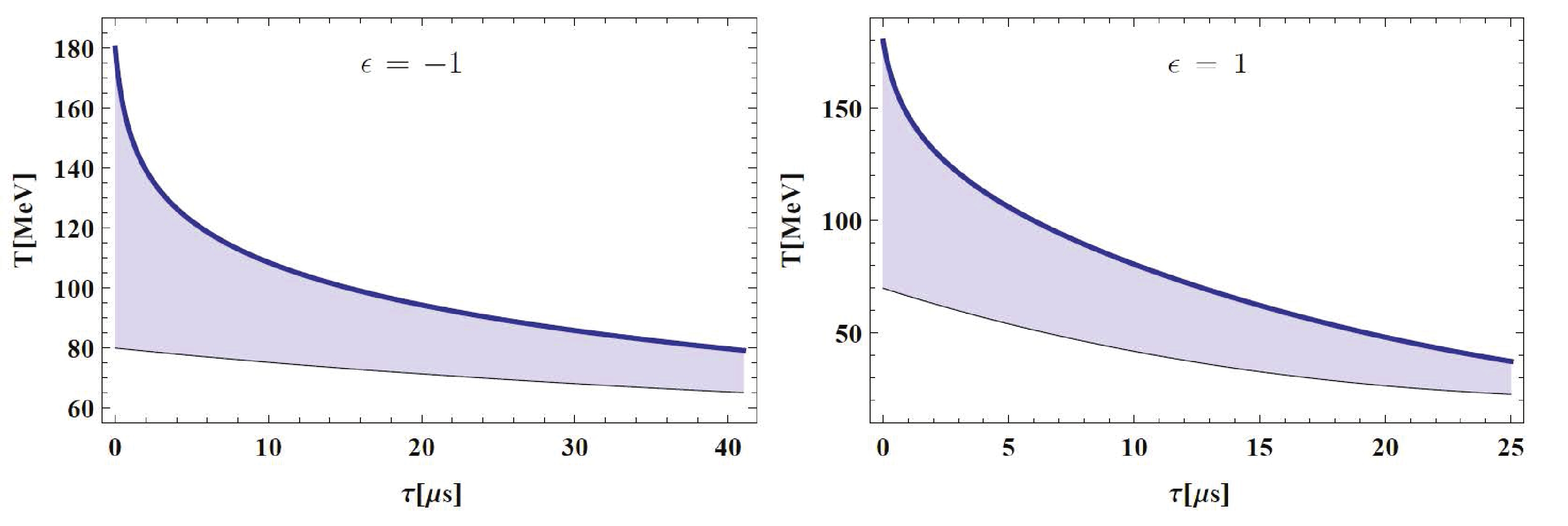
Figure 11. (color online)
$T$ versus$\tau$ in low temperature region by smooth crossover procedure in DGP brane gravity with BD scalar field on brane for$80\;{\rm{MeV}} \leq T \leq 180\;{\rm{MeV}}$ and following constants:$\beta = 2.47 \times 10^{-3}$ ,$\Phi_0 = 2 \times 10^{5}\;{{\rm{MeV}}^{-1}}$ ,$\omega = 10^4$ , and$\lambda = 10^{9}\;{{\rm{MeV}}^4}$ . -
We investigated the quark-hadron phase transition in the Brans-Dicke DGP model of brane gravity by considering two different scenarios. The evolution of physical quantities that are relevant to the physical description of early times was studied, including the energy density, the scale factor, and temperature, for two cases of
$ \epsilon = -1 $ and$ \epsilon = +1 $ , known as normal and self-accelerating branches, respectively, in the original DGP model. The quark-hadron phase transition was investigated using two scenarios as the first-order phase transition and smooth crossover phase transition. The first-order phase transition scenario occurs inthe intermediate temperature range, i.e.,$ 180\;{\rm{MeV}} < T < 250\;{\rm{MeV}} $ . Applying this scenario, the behavior of physical quantities, namely the temperature, energy density, and scale factor, were studied for different stages before (quark-gluon phase), during, and after (hadron phase) the phase transition for both branches of the model as the normal branch and the self-accelerating branch. The result indicates that the universe is expanding during the phase transition, whereas the temperature and pressure are constant, and the universe transitions from a pure quark phase to a pure hadronic phase. The phase transition for this scenario depends on the values of the BD coupling constant, where for higher$ \omega $ we have a faster transition. Further, the phase transition in the self-accelerating branch occurs earlier than the transition in the normal branch.In this case, our results can be compared with [2,51,56,57,58,65,66,76]. The time period of the phase transition that was obtained in [2,76], where the first-order phase transition was studied in the standard gravity model, which is comparable with our result. By choosing a proper value of BD coupling constant, e.g.,
$ \omega_c $ , for our model, we obtain almost the same period of time for the phase transition as in [2,76]. However, for smaller values,$ \omega < \omega_c $ , the phase transition occurs faster in our model. In [58], the authors utilized a RS brane-world framework and considered their results for different values of the brane tension. The phase transition occurs significantly earlier in comparison to our study. Further, the authors considered the brane tension effect on the time of transition, which results in a later transition for a larger value of brane tension. In [56], the authors considered the phase transition in Brans-Dicke brane gravity, and their results are plotted for different values of Brans-Dicke coupling constant, which displays that the transition time increases with a decreasing BD coupling constant. The authors considered the phase transition using a DGP brane scenario, and their results are depicted for different values of brane tension in [51] expressing a later transition for a smaller value of brane tension. In comparison to [51,56], our model predicts that the quark-hadron phase transition lasts longer.In the following part, the QCD phase transition was studied by applying a smooth crossover approach for two regimes of high and low temperatures. In the high-temperature regime, where the temperature is assumed to be larger than
$ 250\;{\rm{MeV}} $ , the trace anomaly is computed accurately, and the outcome determines radiation like behavior for quarks and gluons. However, in the low-temperature regime, where the temperature is supposed to be less than$ 150\;{\rm{MeV}} $ , the trace anomaly is not applicable, as it is affected by a large discretization effect. Instead, the HRG model is utilized to construct a realistic equation of state. The phase transition time in the high-temperature regime is the same for both normal and self-accelerating branches of the model. However, for the low temperature regime, the transition occurs faster for self-accelerating branch. The results of this case can be compared with those of [51,56,57,65,66]. In [56], the authors investigated QHP transition in RS brane-world model including a BD scalar field, and in [51] this was considered for a self-accelerating branch of the DGP brane scenario. The authors found that a transition occurs in a few micro-seconds for both regimes. In [57,65,66], the authors studied the phase transition in the RS brane-world, including a bulk chameleon-like scalar field. This model provides a non-conservation equation of state, and their results indicate that a phase transition happens faster than in our study.
Quark-hadron phase transition in DGP including BD brane
- Received Date: 2019-12-30
- Accepted Date: 2020-03-26
- Available Online: 2020-08-01
Abstract: A Dvali–Gabadadze–Porrati (DGP) brane-world model with perfect fluid brane matter including a Brans-Dicke (BD) scalar field on brane was utilized to investigate the problem of the quark-hadron phase (QHP) transition in early evolution of the Universe. The presence of the BD scalar field arises with several modified terms in the Friedmann equation. Because the behavior of the phase transition strongly depends on the basic evolution equations, even a small change in these relations might lead to interesting results about the time of transition. The phase transition is investigated in two scenarios, namely the first-order phase transition and smooth crossover phase transition. For the first-order scenario, which is used for the intermediate temperature regime, the evolution of the physical quantities, such as temperature and scale factor, are investigated before, during, and after the phase transition. The results show that the transition occurs in about a micro-second. In the following part, the phenomenon is studied by assuming a smooth crossover transition, where the lattice QCD data is utilized to obtain a realistic equation for the state of the matter. The investigation for this part is performed in the high and low-temperature regimes. Using the trace anomaly in the high-temperature regime specifies a simple equation of state, which states that the quark-gluon behaves like radiation. However, in the low-temperature regime, the trace anomaly is affected by discretization effects, and the hadron resonance gas model is utilized instead. Using this model, a more realistic equation of state is found in the low-temperature regime. The crossover phase transition in both regimes is considered. The results determine that the transition lasts around a few micro-seconds. Further, the transition in the low-temperature regime occurs after the transition in the high-temperature regime.


 DownLoad: