


 Abstract
 HTML
HTML Reference
 Related
 PDF
PDF


-
The phase structure of Quantum Chromodynamics (QCD) at high temperature/density and other extreme conditions has attracted a lot of interest and has been the main topic of heavy ion collisions. The perturbative QCD predicts a free gas of quarks and gluons in the high temperature limit, and a color-flavor locking phase at a very high baryon density but low temperature. However, the QCD vacuum has a rather complicated non-perturbative structure, and the QCD phase diagram is not a simple transition from the hadron phase with non-zero chiral condensate to the weakly coupled quark-gluon plasma as expected some time ago [1], but has a rather a rich structure of different phases with corresponding condensates. These phases could include different color superconducting states or inhomogeneous chiral condensates [2-4]. Recently, the QCD phase structure in strong magnetic fields has attracted considerable interest [5-10]. The strong magnetic fields can be generated with a strength of
$ B\sim $ $ 10^{18} $ –$ 10^{20} $ G in non-central heavy ion collisions [6, 11], and are expected to be of the order of$ 10^{18} $ –$ 10^{20} $ G [12, 13] in the inner core of magnetars.At the surface of compact stars, the Coulomb force is essentially balanced by the gravitational force. When the pressure and density of matter inside compact stars are large and the gravitational field is intense, the electric charge distribution is proportional to the mass density. This indicates that a strong electric field (
$ \sim 10^{21} $ –$ 10^{22}\, {\rm V/m} $ ) can be present in compact stars [14]. Moreover, it was suggested that the electrically charged compact stars develop into charged black holes. All these aspects point to the need of studying the QCD matter in the core of compact stars in strong electromagnetic fields, especially in parallel electromagnetic fields. In such a system, new alignment of the QCD vacuum, i.e. neutral pion condensation, could be formed due to the connection of the electromagnetic field with the axial anomaly [15, 16]. If only the QCD interaction is assumed, the axial isospin current is anomaly free. It turns out that the anomaly is associated with the coupling of quarks to the electromagnetic field, where the axial isospin current is given by$ \partial_{\mu}j_{5}^{\,\mu 3} = -\frac{e^{2}}{16\pi^{2}} \varepsilon^{ \alpha \beta\mu\nu}F_{ \alpha \beta}F_{\mu\nu}\cdot {\rm{tr}} \left[\tau_{3}Q^{2} \right]. $

(1) Here, Q is the matrix of quark electric charges,
$ \tau_{3} $ is the Pauli matrix in flavor space and F is the field strength. The corresponding process is$ \pi^{0}\to \gamma \gamma $ . Such a decay of the neutral pion into two photons, which had been a puzzle for some time in the 1960s, is the most successful proof of the chiral anomaly. The above solution led to the discovery of the Adler–Bell–Jackiw anomaly [17].Investigation of the pion condensation in isospin asymmetric nuclear matter has a long history. This effect was first discussed in the case of nuclear matter in neutron star interior [18-20], and superdense and supercharged nuclei [21]. Pion condensation of charged or neutral pion modes in the presence of isospin chemical potential
$ \mu_{I} $ was studied in the lattice QCD [22-25],$ \chi {\rm PT} $ [26-30], hadron resonance gas [31], the random matrix models [32], NJL models [33-46], quark-meson models [4, 47-49], the Dyson-Schwinger approach [50], functional renormalization group [51, 52], topologically large$ N_c $ [53], and the holographic QCD [54, 55]. Recently, the charged pion condensation in the presence of background magnetic fields was discussed in [56-60].The axial isospin chemical potential
$ \mu_{I}^5 $ is introduced because of the presence of the current$ \bar{\psi} \gamma_{0} \gamma_{5}\tau_{3}\psi $ , and is similar to the isospin chemical potential$ \mu_{I} $ which is related to$ \bar{\psi} \gamma_{0}\tau_{3}\psi $ in the asymmetric quark charge space. Generally speaking, any term involving$ \tau_{3} $ flavor operator destroys the degeneracy between$ \pi^{0} $ and$ \pi^{\pm} $ . In QCD matter which includes the coupling between quarks and electromagnetic fields, it is worth pursuing the detailed behavior of charged pions in a strict manner. In the$ \chi {\rm PT} $ approach, the behavior of neutral particles is not modified in the leading order. However, higher order is required to solve the complicated Schroedinger equations for a charged particle in a nonzero electromagnetic field, where$ \chi {\rm PT} $ does not help much. Hence, in this work, we focus on the possibility of charged pion condensation in an anti-parallel electromagnetic field by applying the$ {SU}(2) \times {SU}(2) $ NJL model [61, 62]. For this purpose, we develop a full routine to derive the mean-field thermodynamical potential in the NJL model with nonzero charged pion condensate$ \left\langle { \bar{\psi} {\rm i} \gamma_5 \tau_{\pm} \psi } \right\rangle $ in the off-diagonal flavor space and in anti-parallel electromagnetic fields at finite isospin chemical potential. It should be noted that in order to be certain that the charged pion condensate is energetically preferred, we assume a finite isospin chemical potential$ \mu_I > 0.5 m_\pi $ following the results in Refs. [25, 26, 28-30]. Otherwise, one has to extend the ansatz to possible simultaneous formation of charged and neutral pion condensates, which is beyond the scope of the present study. Moreover, the influence of the finite isospin chemical potential is studied in a perturbative manner.The calculations are performed using the Schwinger proper time method [63] and the proper time regularization in the NJL model [64, 65]. We only consider the model at zero temperature and chemical potential, and restrict our study to the case of the electric field that is anti-parallel to the magnetic field in the presence of isospin chemical potential.
-
The Lagrangian of the
$ {SU}(2)\times {SU}(2) $ NJL model is in the form of [61, 62, 66-70]$ \begin{split}{\cal L}_{ {\rm NJL}} =& \bar{\psi}\left( {\rm i} {\not \!\!\!D} - m_0 +\mu_I\gamma_0\tau_3\right) \psi \\ &+ {G} \left[ \left( \bar{\psi} \psi \right)^2+ \left( \bar{\psi} {\rm i}\gamma_5 \tau_i \psi \right)^2 \right], \end{split} $

(2) where
$ \bar{\psi}(x) = (\bar{u}(x),\bar{d}(x)) $ are u and d anti-quark fields, and G is the four-quark coupling constant. The limit of equal current masses for$ u,d $ ,$ m_u = m_d\equiv m_{0} $ is considered.$ \gamma_i $ ,$ \tau_{i} $ are the conventional Dirac and Pauli matrices and$ \tau_{0} $ is the unit matrix.$ {\not\!\!\! D} $ is the covariant derivative in the two flavor space, expressed as$ D_{\mu} = \left( \partial_{\mu}- {\rm i} QA_{\mu} \right)\tau_{0}- {\rm i} qA_{\mu}\tau_{3}, $

(3) where
$ Q = \frac{1}{2} \left(q_{u}+q_{d} \right) $ and$ q = \frac{1}{2} \left(q_{u}-q_{d} \right) $ .Introducing the auxiliary bosonic fields
$ \pi $ ,$ \sigma $ , with the help of the Hubbard-Stratonovich transformation, one can integrate over the quark fields to obtain the following effective Lagrangian:$ {\cal L} = -\frac{\sigma^2+\vec{\pi}^2}{4 G}- {\rm i} {\rm Tr} \ln \left(S^{-1}+\mu_{I} \gamma_{0}\tau_{3} \right), $

(4) where
$ S^{-1} $ is the inverse quark propagator without the isospin chemical potential, and$ S^{-1} = \mathop{}\!{\rm i} {\not\!\! D} - M, \quad M = m_{0}\tau_{0}-\sigma\tau_{0}- \mathop{}\!{\rm i} \gamma_5\pi_{i} \tau_i. $

(5) We obtain
$ \mu_I $ in a perturbative way, where the$ 4N_{f}\times 4N_{f} $ Dirac matrix in the second term of Eq. (4) is expanded as$ \ln \left(S^{-1}+\mu_I\gamma_0\tau_3 \right) \approx \ln S^{-1} + \frac{\mu_I\gamma_0\tau_3}{S^{-1}}- \frac{\mu_I^2}{2 S^{-2}}. $

(6) The term linear in
$ \mu_I $ vanishes in order to maintain a nonzero Dirac trace because it is linked to odd powers in momentum integration. The higher order terms are ignored. We note that because the NJL model is nonrenormalizable, its physical predictions inevitably depend on the regularization procedure and the model parameters chosen [65]. If the UV momentum cutoff$ \Lambda $ is larger than the isospin chemical potential,$ \mu_{I} $ can be treated perturbatively, which is the case in the whole region of our model calculations.The auxiliary bosonic fields could have a nonzero vacuum expectation values and therefore it is necessary to shift them as
$ \sigma = \sigma^\prime-\left\langle \sigma \right\rangle $ ,$ \pi_{i} = \pi_{i}^\prime- \left\langle {{\pi _i}} \right\rangle $ . The equations of motion for the mean-fields$ \left\langle \sigma \right\rangle $ ,$ \left\langle {{\pi _i}} \right\rangle $ are obtained from the Lagrangian (4) after elimination of the linear terms, i.e.$ \frac{\delta {\cal L} }{\delta \left\langle \sigma \right\rangle }\biggl|_{\substack{ \sigma^\prime = 0 \\ \pi_{i}^\prime = 0 }}, \quad \frac{\delta {\cal L} }{\delta \left\langle {{\pi _i}} \right\rangle }\biggl|_{\substack{ \sigma^\prime = 0 \\ \pi_{i}^\prime = 0 }} = 0. $

(7) As a result, since
$ \left\langle \sigma \right\rangle $ ,$ \left\langle {{\pi _i}} \right\rangle $ condensates have non-zero values, the non-zero value of the scalar condensate leads to a formation of constituent quarks with dynamical quark mass$ m = m_{0}-\left\langle \sigma \right\rangle $ .Let us denote the second term of the effective Lagrangian (4) as
$ {\cal S}_{\rm eff} = - \mathop{}\!{\rm i} {\rm Tr} \ln S^{-1} $ . The gap equations for$ \left\langle \sigma \right\rangle $ and$ \left\langle {{\pi _i}} \right\rangle $ then take the form$ m = m_{0}-2{\rm G}\frac{\partial{\cal S}_{\rm eff}}{\partial \left\langle \sigma \right\rangle },\quad \left\langle {{\pi _i}} \right\rangle = 2{\rm G}\frac{\partial {\cal S}_{\rm eff}}{\partial \left\langle {{\pi _i}} \right\rangle }. $

(8) The calculation of
$ {\cal S}_{\rm eff} $ is presented in the following section. -
As discussed in [35, 36], the
$ {SU}(2)\times{SU}(2) $ symmetry is broken into$ {U}(1)_{I_{3}}\times{U}(1)_{AI_{3}} $ due to the asymmetric$ {U}(1)_{em} $ coupling in flavor space. This leaves two invariant combinations:$ \sigma^{2}+\pi_{3}^{2} $ and$ \pi_{1}^{2}+\pi_{2}^{2} $ . Without loss of generality, one can choose$ \left\langle M \right\rangle = \left(m,\pi_{1},0,0 \right) $ , and therefore the "mass" in the quark propagator Eq. (5) is$ M = m\tau_{0}+ \mathop{}\!{\rm i}\pi_{1} \gamma_{5}\tau_{1} $ . Since$ {\rm Det} \left( \mathop{}\!{\rm i} {\not\!\!\! D} -M \right) = {\rm Det}\, \Gamma \left( \mathop{}\!{\rm i} {\not\!\!\! D} -M \right) \Gamma $ , where$ \Gamma = \gamma_{5}\tau_{3} $ , taking into account Eq. (6), the second term of the Lagrangian Eq. (4) is reduced to$ {\cal S}_{\rm eff} = \frac{- \mathop{}\!\rm i}{2} {\rm Tr}\ln \left( {\not \!\!\!{\cal D}} ^{2}+|M|^2 \right)+\frac{ \mathop{}\!{\rm i}}{2} {\rm Tr}\frac{\mu_I^2}{ {\not\!\!\! {\cal D}} ^{2}+|M|^2}, $

(9) where
$ |M|^2 = m^2+\pi_1^2 $ ,$ {\not\!\!\! {\cal D}} ^{2} = {\not \!\!\!D} ^{2}- \gamma_{5} \gamma^{\mu}\pi_{1} \left[\tau_{1},D_{\mu} \right] $ , and the identity$ {\rm Tr}\ln A = \ln {\rm Det}\,{A} $ has been applied to get Eq. (6).Employing the method of proper time, we represent
$ {\cal S}_{\rm eff} $ as:$ \begin{split} {\cal S}_{\rm eff}=&{{\rm Tr}\int\limits_{1/\Lambda ^{2}}^{\infty}{\rm i}\,\dfrac{{\rm d} s}{2s}(1-\mu_I^2s)}\\ &{\times\int{\rm{tr}}\left\langle {x\big|{\rm e}^{-{\rm i}({\not{\cal D}}^{2}+m^{2}+\pi_{1}^{2})s}\big|y} \right\rangle {\rm d}^{4}x,} \end{split} $

(10) where the ultraviolet cutoff
$ 1/ \Lambda^{2} $ has been explicitly introduced,$ {\rm{tr}} $ and$ {\rm Tr} $ mean that the trace is taken in the spinor and flavor spaces, respectively.Following Schwinger's pioneering work [63], we work in the Euclidean space. The corresponding notation is introduced:
$ \begin{split} \alpha =& m^{2}+\pi_{1}^{2}-\dfrac{1}{2} \sigma^{\mu\nu} \lambda_{\mu\nu},\quad \beta_{\nu} = q\pi_{1} \gamma_{5} \gamma^{\mu}F_{\mu\nu}\tau_{2},\quad \\ \lambda_{\mu\nu} =& q_{f}F_{\mu\nu}, \end{split} $

(11) where
$ q_{f} = {\rm Diag}(q_{u},q_{d}) $ and$ \sigma^{\mu\nu} = \dfrac{ \mathop{}\!{\rm i}}{2} \left[ \gamma^{\mu}, \gamma^{\nu} \right] $ . In order to obtain$ {\cal S}_{\rm eff} $ , it is then straightforward to look for the solution of$ G(x,y;s) $ which obeys the second order differential equation$ \left( {\not\!\!\! {\cal D}} ^{2}+m^{2}+\pi_{1}^{2} \right)G \left(x,y \right) = \delta(x-y) $ . The explicit form is$ \begin{split} {\not \!\!\!{\cal D}} ^{2}+m^{2}+\pi_{1}^{2}\equiv & \partial^{2}_{x}+\alpha(y)+\beta_{\mu}(y) \left(x-y \right)^{\mu}\\ &+\dfrac{1}{4} \lambda^{2}_{\mu\nu} \left(x-y \right)^{\mu} \left(x-y \right)^{\nu}. \end{split}$

(12) Performing the Fourier transform, one finds,
$ \left(-p^{2}+\alpha- \mathop{}\!{\rm i}\beta_{\mu}\frac{ \partial}{ \partial p_{\mu}}-\frac{1}{4} \lambda^{2}_{\mu\nu}\frac{ \partial^{2}}{ \partial p_{\mu} \partial p_{\nu}} \right)G(p;s) = 1. $

(13) As suggested in Ref. [71], one can solve the above equation with
$ G(p;s) = \mathop{}\!{\rm e}^{-\alpha s+ p\cdot A(s)\cdot p+B(s) \cdot p+C(s)}, $

(14) where the matrix A, vector B and scalar C are
$ \begin{split}A =& \lambda^{-1}\tan \lambda s,\quad B = -2 \mathop{}\!{\rm i} \beta\cdot \lambda^{-2} \left(1-\sec \lambda s \right),\\ C =& -\dfrac{1}{2}\, {\rm{tr}}\ln\cos \lambda s- \beta\cdot \lambda^{-3} \left(\tan \lambda s- \lambda s \right)\cdot \beta . \end{split} $

(15) The detailed procedure can be seen in Ref. [71]. For simplicity, the indexes are not shown in the above equations.
Plugging the
$ \beta $ term from Eq. (11) into the vector B and restoring indexes, one has$ B_{\mu} = -2 \mathop{}\!{\rm i} q\pi_{1}\tau_{2} \gamma_{5} \gamma^{\nu}F_{\nu \alpha} \left[ \lambda^{-2} \left(1-\sec \lambda s \right) \right]^{ \alpha}_{\mu}. $

(16) It should be noted that the vector B contains the Dirac matrix, and does not commute with the
$ \sigma^{\mu\nu} \lambda_{\mu\nu} $ term in the expression for$ \alpha $ in Eq. (11). Therefore, one should be careful with the trace in the spinor space and with the integration in the momentum space. Introducing the notation$ P_{1} = \frac{1}{2} \sigma \lambda s $ and$ P_{2} = p\cdot A(s)\cdot p+B(s) \cdot p $ , one has$ \left[ \sigma \lambda s, p\cdot A(s)\cdot p \right] = 0 $ , and the matrices in the exponent in Eq. (14) can be expanded by the Baker-Campbell-Hausdorff formula to second order:$ \begin{split} \mathop{}\!{\rm e}^{P_{1}+P_{2}}\simeq & \mathop{}\!{\rm e}^{P_{1}} \mathop{}\!{\rm e}^{P_{2}} \mathop{}\!{\rm e}^{-\frac{1}{2}[P_{1},P_{2}]} \\ =& \mathop{}\!{\rm e}^{\frac{1}{2} \sigma \lambda s} \mathop{}\!{\rm e}^{p\cdot A(s)\cdot p+B(s) \cdot p} \mathop{}\!{\rm e}^{-\frac{1}{4} \left[ \sigma \lambda s,B(s) \cdot p \right]}. \end{split} $

(17) The higher order terms can be ignored since
$ B(s) \cdot p\sim \pi_{1}p/\Lambda^{2}\ll 1 $ , which will be examined later.We denote
$ -\frac{1}{4} \left[ \sigma \lambda s,B(s) \cdot p \right] = \frac{1}{2}q\pi_{1} Os $ , where O is of the form$ O = Q\tau_{2}O_{1}\mathbb{B}_{1}p+q\tau_{1}O_{2}\mathbb{B}_{2}p $ , and$ \mathbb{B} $ is given in Eq. (19). The shorthand matrix notation is applied, i.e.$ \mathbb{F} = F_{\mu}^{\nu} $ , with index raising$ g^{ \alpha\mu}F_{\mu}^{\nu} = F^{ \alpha\nu} $ . To find the eigenvalues of O, we take the square [63] and get:$ \begin{split} O^{2} =& Q^{2} \left(\tau_{2}O_{1}\mathbb{B}_{1}p \right)^{2}+q^{2} \left(\tau_{1}O_{2}\mathbb{B}_{2}p \right)^{2} \\ &- \mathop{}\!{\rm i} qQ\tau_{3} \left[O_{1}\mathbb{B}_{1}p,O_{2}\tilde{\mathbb{B}}_{2}p \right],\\ \;\;O_{1} =& \mathop{}\!{\rm i} \left[ \sigma_{\mu\nu}, \gamma_{5} \gamma^{ \alpha} \right] = 2 \gamma_{5}g_{\nu}^{ \alpha} \gamma_{\mu}-2 \gamma_{5}g_{\mu}^{ \alpha} \gamma_{\nu},\\ \;\;O_{2} =& \left\{ \sigma_{\mu\nu}, \gamma_{5} \gamma^{ \alpha} \right\} = -2 \varepsilon^{ \alpha \beta}_{\;\mu\nu} \gamma_{ \beta}. \end{split}$

(18) With the help of
$ \tau_{2}q_{f}\tau_{2} = {\rm Diag} \left(q_{d}, q_{u} \right) = \tilde{q}_{f} $ ,$ \tilde{\mathbb{B}} \left(\mathbb{B} \right) $ are obtained as$ \begin{split}\tilde{\mathbb{B}}_{1} \left(\mathbb{B}_{1} \right) =& \frac{1}{{\mathsf q}^{2}} \left[1-\sec {\mathsf q}\mathbb{F}s \right],\quad \\ \tilde{\mathbb{B}}_{2} \left(\mathbb{B}_{2} \right) =& \frac{\bar{\mathbb{F}}\mathbb{F}}{\mathbb{F}^{2}} \frac{1}{{\mathsf q}^{2}} \left[1-\sec{\mathsf q}\mathbb{F}s \right], \end{split} $

(19) where
$ {\mathsf q} = \tilde{q}_{f} $ or$ q_{f} $ for$ \tilde{\mathbb{B}},\mathbb{B} $ , respectively;$ \mathbb{F} $ and$ \bar{\mathbb{F}} $ are the field strength tensor$ F^{\mu\nu} $ and the dual field strength tensor$ \bar{F}^{\mu\nu} = \frac{1}{2} \varepsilon^{\mu\nu \alpha \beta}F_{ \alpha \beta} $ in shorthand notation. Moreover,$ \left(\tau_{2}O_{1}\mathbb{B}_{1}p \right)^{2} = -16\mathbb{B}_{1}\tilde{\mathbb{B}}_{1}p^{2} $ ,$ \left(\tau_{1}O_{2}\mathbb{B}_{2}p \right)^{2} = 16\mathbb{B}_{2}\tilde{\mathbb{B}}_{2}p^{2} $ and$ [O_{1}\mathbb{B}_{1}p,O_{2}\tilde{\mathbb{B}}_{2}p] = -32 \gamma_{5}\mathbb{B}_{1}\tilde{\mathbb{B}}_{2}p^{2} $ .In the Lorentz frame with the anti-parallel electromagnetic field vectors, e.g.
$ {\bf{B}} = - {\bf{E}} = f\hat{z} $ , one gets$ \mathbb{F}^{2} = f^2\, {\rm Diag} \left(-,+,+,- \right) $ and$ \bar{\mathbb{F}}\mathbb{F} = -f^2 \delta_{\mu\nu} $ in the Euclidean metric$ (-,-,-,-) $ , so that$ \bar{\mathbb{F}}\mathbb{F}/\,\mathbb{F}^{2} = f^{2}\mathbb{F}^{-2} $ . Besides,$ \left[1-\sec{\mathsf q}\mathbb{F}s \right] $ contains even powers of$ \mathbb{F} $ . As a result$ O^{2} = -16Q^{2}{\mathsf p}_{1}^{2}+16q^{2}{\mathsf p}_{2}^{2}+32 \mathop{}\!{\rm i} qQ\tau_{3} \gamma_{5}{\mathsf p}_{1}\cdot{\mathsf p}_{2}, $

(20) where
$ {\mathsf p}_{1} = p_{\shortparallel}+p_{\perp} $ ,$ {\mathsf p}_{2} = p_{\shortparallel}-p_{\perp} $ ,$ p_{\shortparallel} = b_{\shortparallel}(p_{0},0,0,p_{3}) $ and$ p_{\perp} = b_{\perp}(0,p_{1},p_{2},0) $ , because$ {\mathsf p}_{1}^{2} = {\mathsf p}_{2}^{2} = -p_{\shortparallel}^{2}-p_{\perp}^{2} $ and$ {\mathsf p}_{1}\cdot{\mathsf p}_{2} = -p_{\shortparallel}^{2}+p_{\perp}^{2} $ in the Euclidean metric.$ b_{\shortparallel} $ and$ b_{\perp} $ are:$ b_{\shortparallel} = \frac{(1-\sec q_{f}s)^{\frac{1}{2}}(1-\sec\tilde{q}_{f}s)^{\frac{1}{2}}}{q_{f}\tilde{q}_{f}}, $

(21) $ b_{\perp} = \frac{(1-{\rm{sech}}\; q_{f}s)^{\frac{1}{2}}(1-{\rm{sech}}\;\tilde{q}_{f}s)^{\frac{1}{2}}}{q_{f}\tilde{q}_{f}}. $

(22) Here and below, we rescale the integration variable as
$ s = s^\prime/f $ and omit the prime. Since$ \gamma_{5}^{2} = 1 $ is associated with the eigenvalue$ \pm 1 $ , it follows that O has four eigenvalues in the Dirac space [63], written as$ {\cal O} = \pm 4 \left( \mathop{}\!i Q{\mathsf p}_{1}\pm q\tau_{3}{\mathsf p}_{2} \right). $

(23) Letting
$ \theta = q\pi_{1} s/f $ and applying the results of Eq. (23), we have$ {\rm{tr}}\, \mathop{}\!{\rm e}^{\frac{1}{2} \theta O} = {\mathsf T} = \cos \left(2Q \theta{\mathsf p}_{1} \right)\cosh \left(2\tau_{3}q \theta{\mathsf p}_{2} \right), $

(24) where we adopt the method applied in [72]. Let
$ K^{2} = {\mathsf p}_{1}^{2} = {\mathsf p}_{2}^{2} $ , the full relation is:$ \exp \left[\frac{1}{2} \theta O \right] = {\mathsf T}+ \mathop{}\!{\rm i} \gamma_{5}{\mathsf U}+\frac{O{\mathsf V}}{2K^{2}}+\frac{ \mathop{}\!{\rm i} \gamma_{5}O{\mathsf W}}{2K^{2}}, $

(25) where
$ {\mathsf T}, {\mathsf U}, {\mathsf V} $ and$ {\mathsf W} $ are scalars, which we write explicitly below. We take the following result from [72], :$ \exp \left[q_{f}\frac{ \sigma Fs}{2f} \right] = {\mathsf P}- \mathop{}\!{\rm i} \gamma_{5}{\mathsf Q}+\frac{ \sigma F}{2f}\,{\mathsf R}-\frac{ \mathop{}\!{\rm i} \gamma_{5} \sigma F}{2f}\,{\mathsf S}. $

(26) Since
$ {\rm{tr}} \left(O^{2} \mathop{}\!{\rm e}^{\frac{1}{2} \theta O} \right) = \frac{ \partial^{2}}{ \partial^{2} \theta} {\rm{tr}} \left(4 \mathop{}\!{\rm e}^{\frac{1}{2} \theta O} \right) = 4\frac{ \partial^{2}{\mathsf T}}{ \partial^{2} \theta}, $

(27) we get from Eq. (24),
$ {\mathsf U} = \sin \left(2Q \theta{\mathsf p}_{1} \right)\sinh \left(2\tau_{3}q \theta{\mathsf p}_{2} \right). $

(28) Proceeding with the direct differentiation of the exponential function as in [72], we get
$ \begin{split}{\mathsf V} =& \frac{1}{Q^{2}+q^{2}} \biggl(Q{\mathsf p}_{1}\sin \left(2Q \theta{\mathsf p}_{1} \right)\cosh \left(2\tau_{3}q \theta{\mathsf p}_{2} \right)\\ &+\tau_{3}q{\mathsf p}_{2}\cos \left(2Q \theta{\mathsf p}_{1} \right)\sinh \left(2\tau_{3}q \theta{\mathsf p}_{2} \right)), \\ {\mathsf W} =& \frac{1}{Q^{2}+q^{2}} \biggl(\tau_{3}q{\mathsf p}_{2}\sin \left(2Q \theta{\mathsf p}_{1} \right)\cosh \left(2\tau_{3}q \theta{\mathsf p}_{2} \right)\\ &-Q{\mathsf p}_{1}\cos \left(2Q \theta{\mathsf p}_{1} \right)\sinh \left(2\tau_{3}q \theta{\mathsf p}_{2} \right)).\end{split} $

(29) From [72], one has
$ \begin{split}{\mathsf P} = &\cos q_{f}s\cosh q_{f}s,\, {\mathsf Q} = \sin q_{f}s\sinh q_{f}s ,\\ {\mathsf R} =& (\sinh q_{f}s\cos q_{f}s+\cosh q_{f}s\sin q_{f}s)/2,\\ {\mathsf S} =& (\sinh q_{f}s\cos q_{f}s-\cosh q_{f}s\sin q_{f}s)/2. \end{split}$

(30) To perform the momentum integration, we expand the exponential function as
$ \mathop{}\!{\rm e}^{ p\cdot A(s)\cdot p+B(s)\cdot p} = \mathop{}\!{\rm e}^{ p\cdot A(s)\cdot p} \left(\cos\varrho+B(s) \cdot p\frac{\sin\varrho}{\varrho} \right), $

(31) where
$ \varrho = 2q\pi_{1}k/f $ and$ k = \sqrt{{\mathsf p}_{1}\cdot{\mathsf p}_{2}} $ .We can now integrate with respect to p and take the trace in the spinor space. Recalling Eq. (17), we get:
$ \begin{split} L(s) =& {\rm{tr}}\int \mathop{}\!{\rm e}^{\frac{1}{2f} \sigma \lambda s} \mathop{}\!{\rm e}^{p\cdot A(s)\cdot p+B(s)\cdot p} \mathop{}\!{\rm e}^{-\frac{1}{4f} \left[ \sigma \lambda s,B(s) \cdot p \right]} \mathop{}\!{\rm d}^{4}p \\ =& L_{0}(s)+L_{1}(s)+L_{2}(s). \end{split} $

(32) Denoting by
$ \left\langle X \right\rangle $ the result of integration and the trace$ {\rm{tr}}\int X \mathop{}\!{\rm e}^{p\cdot A\cdot p} \mathop{}\!{\rm d}^{4}p $ , and substituting into Eq. (25), Eq. (26) and Eq. (31), we get$ \begin{split} {L_0}(s) =& {\left\langle {\cos \varrho {\mathsf T}{\mathsf P}} \right\rangle ,\; {L_1}(s) = \left\langle {\cos \varrho {\mathsf U}{\mathsf Q}} \right\rangle ,}\\ {L_2}(s) = & {\left\langle {\frac{{2{{\tilde q}_f}\sin \varrho }}{{{K^2}k}}\left[ {{q_f}{K^2}\left( {{\mathsf W}{\mathsf S}- {\mathsf V}{\mathsf R}} \right) + {{\tilde q}_f}{k^2}\left( {{\mathsf V}{\mathsf S} + {\mathsf W}{\mathsf R}} \right)} \right]} \right\rangle .} \end{split}$

(33) The integral with respect to momentum p is in the form of a Gaussian, which can be easily evaluated as:
$ \begin{split} \left\langle {1} \right\rangle =& {\cal N} = \pi^{2} {\rm Det}A^{-\frac{1}{2}}\;{\rm for}\; A = {\rm Diag} \left(a_{\shortparallel}, a_{\perp}, a_{\perp}, a_{\shortparallel} \right),\\ \left\langle {K^{2}} \right\rangle =& \frac{{\cal N}}{2}\, {\rm{tr}} \left(\frac{D_{+}}{A} \right),\; \left\langle {k^{2}} \right\rangle = \frac{{\cal N}}{2}\, {\rm{tr}} \left(\frac{D_{-}}{A} \right) . \end{split}$

(34) The matrices
$ D_{\pm} = {\rm Diag} \left(b^{2}_{\shortparallel}, \pm b^{2}_{\perp}, \pm b^{2}_{\perp}, b^{2}_{\shortparallel} \right) $ and$ b_{\shortparallel},b_{\perp} $ are given in Eq. (21) and Eq. (22). From Eq. (15), one has$ a_{\shortparallel} = \tan q_{f}s/ \left(q_{f} f \right) $ and$ a_{\perp} = \tanh q_{f}s/ \left(q_{f} f \right) $ . The higher order corrections$ \left\langle {K^{4}} \right\rangle $ ,$ \left\langle {k^{4}} \right\rangle $ and$ \left\langle {k^{2}K^{2}} \right\rangle $ can be obtained in a similar manner.In obtaining Eq. (17), we have applied the argument that
$ B(s) \cdot p\sim \theta p $ is much smaller than 1. The reason is that for small s,$ \theta p\sim\pi_{1}ps/f\sim \pi_{1}p/ \Lambda^{2}\ll 1 $ , while the integration for large s is exponentially suppressed, and hence ignored. This enables to use the approximations$ \sin(a \theta p) $ ,$ \sinh(a \theta p)\sim a \theta p $ and$ \cos(a \theta p) $ ,$ \cosh(a \theta p)\sim 1 $ . Hence,$ {\mathsf T}\sim 1 $ ,$ {\mathsf U}\sim k^{2}s $ ,$ {\mathsf V}\sim K^{2}s $ and$ {\mathsf W}\sim K^{2}k^2 s $ . Finally, applying the term in C in Eq. (15), on has$ \begin{split}{\cal S}_{\rm eff} = &{\cal S}_{\rm eff}^{0}+ {\cal S}_{\rm eff}^{1}+ {\cal S}_{\rm eff}^{2}, \\ {\cal S}_{\rm eff}^{i} = &\frac{N_c }{4\pi^{2}} {\rm Tr}\int_{f/ \Lambda^{2}}^{\infty} \frac{ \mathop{}\!{\rm d} s}{2s} \left(1-\mu_I^2s \right) \mathop{}\!{\rm e}^{-h(s)} S_{\rm eff}^{i}(s),\quad \end{split}$

(35) where
$ -h(s) = -(m^{2}+\pi_{1}^{2})s/f+{C}(s)-\frac{1}{2}\ln {\rm{tr}}{A} $ , and$ \frac{1}{2}\ln {\rm{tr}}{A} $ is obtained from$ {\cal N} $ . Explicitly,$ \begin{split}{C}(s)-\frac{\ln {\rm{tr}}{A}}{2} =& -\ln\frac{\sin q_{f}s\sinh q_{f}s}{q_{f}^{2}f^{2}}\\ &-\frac{2q^{2}{\pi_{1}}^{2}}{\tilde{q}_{f}^{3}f} \left(2\tilde{q}_{f}s-\tan \tilde{q}_{f}s-\tanh \tilde{q}_{f}s \right). \end{split}$

(36) The integrands
$ S_{\rm eff}^{i}(s) $ are$ \begin{split}S_{\rm eff}^{0}(s) = &{\mathsf P},\quad \\ S_{\rm eff}^{1}(s) =& 4 \tau_{3} \frac{Q q^3\pi_{1}^2 s^2}{f^2 {\cal N}}\frac{}{} \left\langle { k^2 } \right\rangle {\mathsf Q} ,\quad \\ S_{\rm eff}^{2}(s) =& \frac{8\tilde{q}_{f}q^2\pi_{1}^2 s}{f^2 {\cal N}} \left(-q_{f} \left\langle { K^2 } \right\rangle {\mathsf R}+\tilde{q}_{f} \left\langle { k^2 } \right\rangle {\mathsf S} \right) \\ &+\tau_{3} \frac{32\tilde{q}_{f} Qq^5 \pi_{1}^4 s^3}{3f^4 {\cal N}} \left(q_{f} \left\langle { K^2k^2 } \right\rangle {\mathsf S}+\tilde{q}_{f} \left\langle { k^4 } \right\rangle {\mathsf R} \right). \end{split} $

(37) The effective potential finally takes the following form:
$ \Omega = \frac{(m-m_{0})^2+\pi_1^2}{4{\rm G}} + {\cal S}_{\rm eff}. $

(38) -
As mentioned, the UV cut-off scheme should be employed in the NJL model to get a reasonable result. In this work, the proper time regularization scheme is applied, i.e. the integration with respect to s starts from
$ f/ \Lambda^{2} $ . We perform the numerical integration of$ {\cal S}_{\rm eff} $ in Eq. (35) and adopt the model parametrizations from Ref. [65]. There are five sets of parameters for proper time regularization in [65] which are fitted to the pion mass and the weak pion decay constant. In order to investigate the dependence of our results on the model parameters, we take the sets with the lowest (set A) and the highest (set B) constituent quark masses. The constituent quark masses for other parameterizations are in between these two cases. In set A, the constituent quark mass is$ 178 $ MeV, and in set B it is$ 372 $ MeV. For convenience, we present the parameter sets in Table 1. Generally, one can consider sets A and B as the limiting cases for the NJL predictions.Set $ m_0 $ /MeV

$ \Lambda $ /MeV

G/GeV-2 m/MeV A 3.0 1464 1.61 178 B 15.0 645 17.2 372 The most important point in the calculations is that the integrands of
$ {\cal S}_{\rm eff} $ contain singularities and one should specify how to deal with them. The singularities are generated either by the trigonometric functions tangent and cotangent of$ q_{i} s $ for quark flavors$ i = u,d $ which lie along the real axis, or by the hyperbolic functions along the imaginary axis. We shift s to the complex plane$ s-i\epsilon $ to avoid crossing the singularities, as shown in Fig. 1. Here, the infinitesimal shift defines the sign of the imaginary part. The imaginary and real parts are obtained at the same time after numerical integration, which is different from the residue summation method used in [64, 73]. Another popular way is to take the integration path as a line from$ f/\Lambda^2 $ with the slope of around$ \pi/4 $ . Taking the advantage of the fact that the contribution of the large (infinite) arc s is zero, and that both the trigonometric and hyperbolic functions in the integrand oscillate less for$ s = |s| \mathop{}\!{\rm e}^{ \mathop{}\!{\rm i}\frac{\pi}{4}} $ , the total integrals converge quickly. A possible issue could be that the proper time regularization scheme may not be applicable and that another regularization scheme must be used in this method. Further discussion of the regularization scheme is beyond the scope of this work.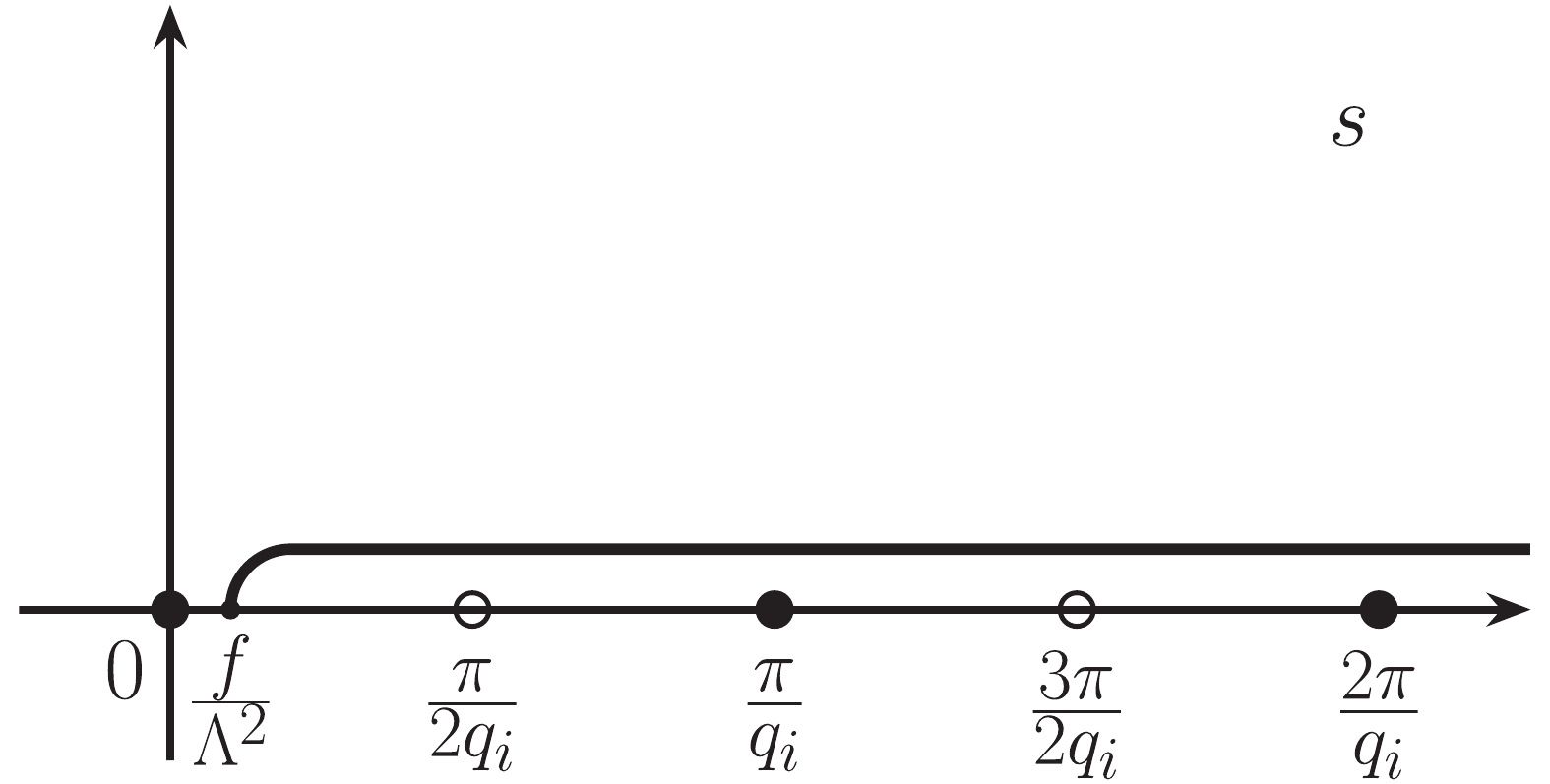
Figure 1. Contour of the complex s-plane. Singularities for a quark of flavor i related to the tangent are shown by open circles, while the filled circles correspond to those related to the cotangent
$ \cot(q_i s) $ .In the right panels of Figs. 2, 3, 4, the effective potential is shown as a "heatmap" in the
$ 2d $ -plane of quark mass m and$ \pi_{1} $ for$ \mu_I = m_\pi $ , field values$ f = 0.01,0.2,0.450 $ GeV2 and set B model parameters. The darkest point is the global minimum that we are searching for. To illustrate the evolution of the global minimum more clearly, we plot the behavior of the potential as a function of m for the values of$ \pi_1 = 0 $ GeV (black solid line),$ 0.2 $ GeV (red dotted),$ 0.45 $ GeV (blue dashed) on the left side of the corresponding figures. We found the following typical behavior in the three regions: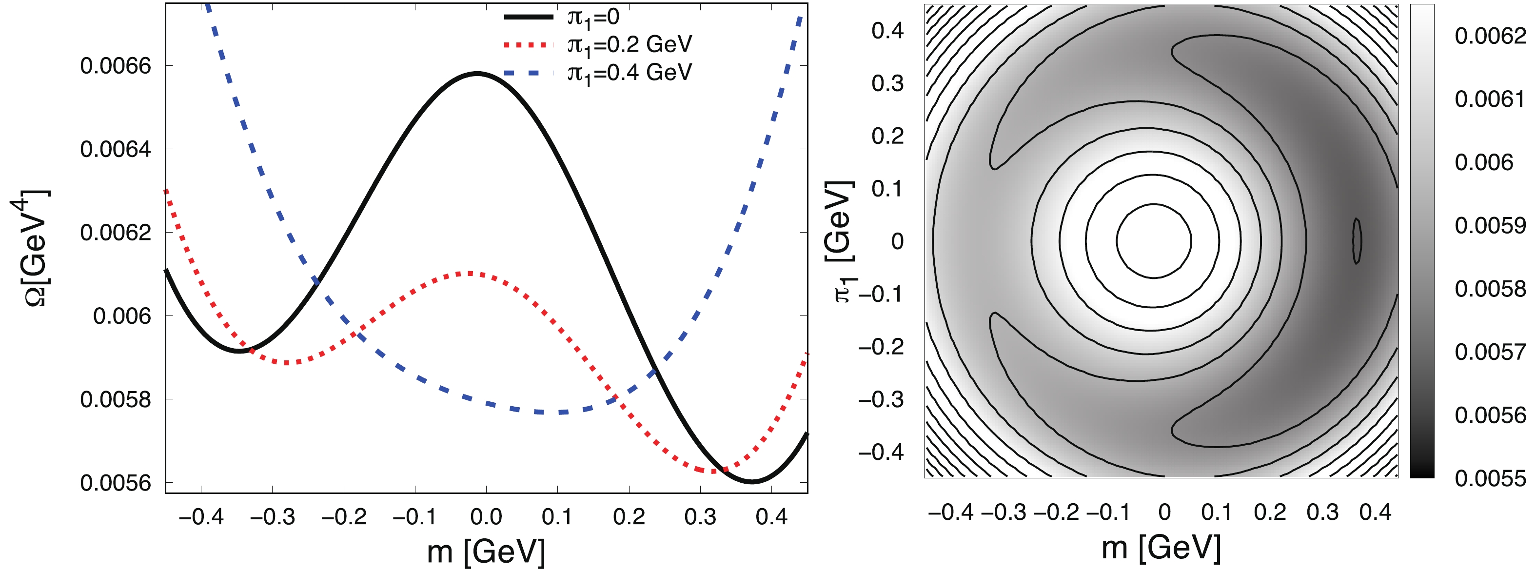
Figure 2. (color online) Behavior of the effective potential in the case of set B, field value
$ f = 0.01 $ GeV2 and$ \mu_I = m_\pi $ , as a function of the quark mass for fixed values of$ \pi_1 $ (left plot), and as a function of the mass and$ \pi_1 $ (right plot). In the left plot, the black solid line corresponds to zero$ \pi_1 $ , red dotted to$ \pi_1 = 0.2 $ GeV, and blue dashed to$ 0.4 $ GeV.
Figure 3. (color online) Behavior of the effective potential in the case of set B, field
$ f = 0.2 $ GeV2 and$ \mu_I = m_\pi $ , as a function of the quark mass for fixed values of$ \pi_1 $ (left plot), and as a function of the mass and$ \pi_1 $ (right plot). In the left plot, the black solid line corresponds to zero$ \pi_1 $ , red dotted to$ \pi_1 = 0.2 $ GeV and blue dashed to$ 0.4 $ GeV. The region in the center of the right plot is omitted because for small m and$ \pi_1 $ the corrections are nonphysical.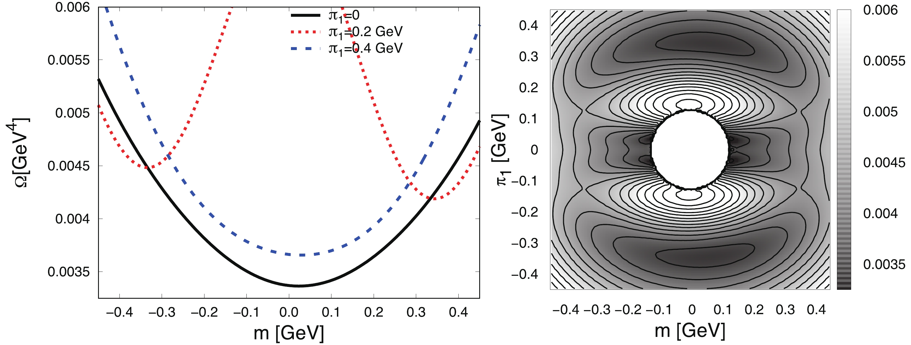
Figure 4. (color online) Behavior of the effective potential in the case of set B, field value
$ f = 0.45 $ GeV2 and$ \mu_I = m_\pi $ , as a function of the quark mass for fixed values of$ \pi_1 $ (left plot), and as a function of the mass and$ \pi_1 $ (right plot). In the left plot, the black solid line corresponds to zero$ \pi_1 $ , red dotted to$ \pi_1 = 0.2 $ GeV and blue dashed to$ 0.4 $ GeV. The region in center of the right plot is omitted because for small but nonzero m and$ \pi_1 $ the corrections are nonphysical.1) For a small field
$ f = 0.01 $ $ {\rm GeV}^2 $ , shown in Fig. 2, we get the usual asymmetric "mexican hat" in the$ m -\pi_1 $ plane. Due to the nonzero current quark mass, the "hat" is tilted and the single global minimum is located at a positive m and zero$ \pi_1 $ (black solid line). However, one can see that there is a very close local minimum at finite$ \pi_1 $ (red dotted line), which indicates that the condensate$ \pi_{1} $ is a competitor with the total order parameter of chiral symmetry breaking of$ |M| = \sqrt{m^2+\pi_1^2} $ near the quark mass in vacuum. In conclusion, the system is in the conventional (almost vacuum) chiral symmetry breaking phase with nonzero sigma condensate and zero pion condensate.2) For a moderate field
$ f = 0.2 $ $ {\rm GeV}^2 $ , shown in Fig. 3, instead of the above global minimum for zero$ \pi_1 $ , the global minimum of the effective potential appears at finite$ \pi_{1} $ , associated with the chiral rotation of the whole system in the$ m -\pi_1 $ plane. This is clearly seen on the left side of Fig. 3, where the red dotted line$ \pi_1 = 0.2 $ GeV is below the black solid line for zero$ \pi_1 $ .3) For a large field
$ f = 0.450 $ $ {\rm GeV}^2 $ , shown in Fig. 4, the minimum with a nonzero$ \pi_1 $ still exists, but the minimum with$ \pi_1 = 0 $ is energetically more favorable since the electromagnetic coupling of charge particles overcomes the chiral anomaly effect, which takes place in the pion space, so that they are back in the normal neutral sigma condensate.There are two sources of chiral symmetry breaking: the spontaneous chiral symmetry breaking due to the presence of the quark condensate
$ \left\langle {\bar{\psi} \psi } \right\rangle $ , and the explicit chiral symmetry breaking due to the nonzero current quark mass in the Lagrangian. We further investigate the physical situation with nonzero quark mass and also for$ m_0\to 0 $ . To systematically perform this task, we vary$ m_{0} $ and recalculate m with the same values of$ {\rm G} $ and$ \Lambda $ , i.e. we consider m as a function of$ m_{0} $ [74]. In the following, we denote the physical value of the current quark mass as$ m_{0}^\star $ .The behavior of m and
$ \pi_1 $ as a function of the field f is presented in Fig. 5 for different values of the ratio$ m_{0}/m_{0}^\star = 0.01,0.1,0.5,1.0 $ and$ \mu_I = m_\pi,1.5 m_\pi,2 m_\pi $ . The left and right sides are for model parameter sets A and B, respectively. For set A and the physical value of the current quark mass$ m_{0}/m_{0}^\star = 1.0 $ , the region of pion condensation is small and the system only slightly rotates in the$ m-\pi_1 $ plane. As the current quark mass decreases, the pion condensation increases. Larger isospin chemical potential leads to a slight increase of the area of pion condensation. For set B, the space of pion condensation is substantially enlarged and is more pronounced. For a moderate field strength, the system rotates to a state where almost all chiral symmetry breaking is in the form of pion condensate. A larger isospin chemical potential noticeably enhances the domain of pion condensation.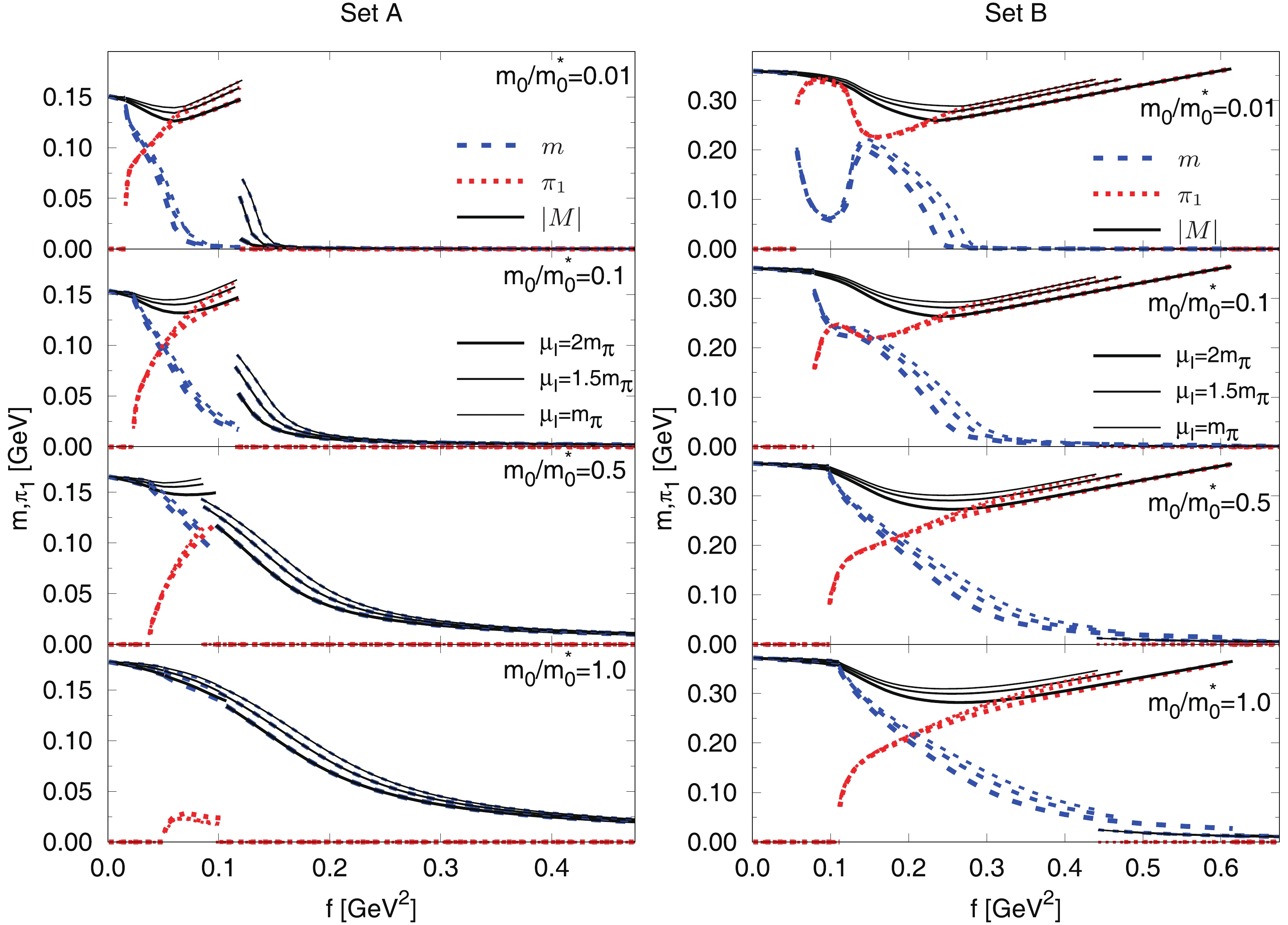
Figure 5. (color online) Behavior of the quark mass m (blue dashed line), pion condensate
$ \pi_1 $ (red dotted line) and their combination$ |M| = \sqrt{m^2+\pi_1^2} $ (black solid line) as a function of field f for sets A and B, and for different values of the ratio of the current quark mass to its physical value$ m_0/m_0^\star = 0.01,0.1,0.5,1.0 $ . The width of the lines corresponds to different values of$ \mu_I $ =$ m_\pi $ (thin),$ 1.5m_\pi $ and$ 2 m_\pi $ (thick).It is straightforward to conclude that for both sets of model parameters and with a small current quark mass it is more preferable for the system to rotate from the sigma axis to the
$ \pi_1 $ direction, accompanied with an unchanged total order parameter of the chiral symmetry breaking$ |M| = \sqrt{m^2+\pi_1^2} $ . As$ m_{0} $ is increased, the phenomenon of chiral rotation becomes less noticeable. It is well known that the current mass of the quarks plays an important role in determining the behavior of the phase transition in QCD matter. Further investigations using the first principle calculations, such as the Dyson-Schwinger equation or the functional renormalization group methods, should be performed.In principle, the effective potential at finite f acquires an imaginary part which corresponds to the pair production due to the Schwinger mechanism [63, 75, 76]. Although the electric field leads to an unstable vacuum, the magnetic field could influence the masses of charged particles which may reduce the decay rate. We find that the imaginary part is smaller than the real part for fields below
$ f_c\sim $ 0.4$ {\rm GeV}^2 $ and sets A and B. Above the critical field value,$ f_{c} $ , when the imaginary part is larger than the real part, the effect of back-reaction of charged pair creation on the electric field is not negligible. For set A,$ f_{c} $ is safely behind the chiral symmetry breaking phase. For set B, the absolute value of$ f_{c} $ changes slightly, but its position shifts to an intermediate position where the whole chiral condensate still exists because the chiral symmetry is restored at a larger field strength than given by the model parameters. We also find that the isospin chemical potential increases the imaginary part, which is unexpected. This is due to the proper time regularization scheme and the UV cutoff,$ f/ \Lambda^{2} $ . One can see from Eq. (10) that the first term of$ {\cal S}_{\rm eff} $ is proportional to$ \int_{f/ \Lambda^{2}}^{\infty}\frac{1}{s} \mathop{}\!{\rm e}^{-h(s)} \mathop{}\!{\rm d} s $ , while the second is$ \sim\mu_{I}^{2} \int_{f/ \Lambda^{2}}^{\infty} \mathop{}\!{\rm e}^{-h(s)} \mathop{}\!{\rm d} s $ . Since the upper limit of s is infinite, the first term is not only exponentially suppressed by$ -h(s) $ at large s , but is also damped by$ 1/s $ . On the other hand, if$ \mathop{}\!{\rm e}^{-h(s)} $ oscillates and the integral converges slowly, then the term proportional to$ \mu^{2}_{I} $ is not damped by$ 1/s $ , and the imaginary part significantly increases for large s .It is not reasonable to take into account the Schwinger effect before such an artificial increment of the imaginary part induced by
$ \mu_{I} $ is removed. Therefore, we draw our conclusions based only on the real part of the numerical results. -
In this paper, the charged pion condensation in anti-parallel electromagnetic fields was studied in the framework of the NJL model by applying the Schwinger proper time method. The configuration of the field, where the electric field is anti-parallel to the magnetic field, was chosen to obtain a zero first Lorentz invariant
$ I_{1} = {\bf{E}}^{2}-{\bf{B}}^{2} $ , and a nonzero second Lorentz invariant$ I_2 = {\bf{E}} \cdot {\bf{B}} $ . In such a configuration, zero$ I_1 $ simplifies the analytical calculations, e.g.$ {\rm{tr}} \left({D_{-}}/{A} \right) = 0 $ in Eq. (34) in the weak f limit. Besides, the parallel and anti-parallel configurations are indeed the same in this work.The Schwinger proper time method was developed to study charged particles moving in either a constant or planar electromagnetic field [63, 77]. The obtained propagators are expressed in an integral form, and are much more complicated than for the freely moving particles. If one is interested in quantities that trivially depend on flavor, i.e. located on the diagonal in flavor space, the propagators are easily expanded in terms of particle charges. However, it is not simple to extract the information in the off-diagonal flavor space where a
$ 4N_{f}\times 4N_{f} $ Dirac matrix must be fully addressed. In this work, following the Schwinger proper time method, we developed a method to solve exactly the$ 4N_{f}\times 4N_{f} $ matrix and to get the corresponding propagators. With the full propagators, it is possible to explore the physical phenomena involving the off-diagonal flavor operators, such as the behavior of a charged pion in an electromagnetic field, where the pion is identified as a bound state of the quark degrees of freedom and not as a point-like charged particle. In order to study the properties of the charge pion condensation, we included a finite isospin chemical potential to avoid competition with the neutral pion.We found that in the chiral limit, the system is preferably formed in a state of nonzero condensation of scalar and charged pions, i.e. by rotating in the chiral group. Chiral condensates aligned in the pseudo mesons space were found in [15] using the method of
$ \chi {\rm PT} $ and the NJL model, but in the chiral limit the system immediately straightens in the$ \pi^0 $ direction once the second Lorentz invariant$ I_2 $ is turned on. The main difference of the charged pion condensation is that the system first crosses a weak first order phase transition to the zero pion condensate, and then undergoes a second order phase transition to the chirally symmetric phase as the field strength increases, while$ \pi^{0} $ is the complete second order phase transition as shown in [15]. The underlying mechanism has two aspects. The first is the obvious coupling between charged pions and electromagnetic field. The other is that a more complicated influence of anomalous diagrams is implicitly included, not only$ \pi^0\rightarrow\gamma\gamma $ but also$ \gamma\gamma\rightarrow \pi^+\pi^-\pi^0 $ [78, 79]. The neutral pion condensate is absent since we are in the region$ \mu_I>m_\pi $ where it has been shown that charged pion condensation is preferable [4, 23, 25-33, 37-55]. A full ansatz containing both the neutral and charged pions will be studied in our next work.More precisely, from the point of view of the Ginzburg-Landau theory [80], if one assumes that the effective potential in the neutral
$ \sigma $ channel is$ {\cal S}_{\rm eff}^{0}\sim -c_{0}M^{2}+c_{1}M^{4}/f $ , which characterizes a second order phase transition, the additional potential from Eq. (35) is:$ {\cal S}_{\rm eff}^{2}\sim -\tilde{c}_{1}M^{4}/f+c_{2}M^{6}/f^{2} $ . Hence, the full effective potential in terms of charged pions is$ \Omega = \frac{M^{2}}{4 {\rm G}}-c_{0}M^{2}+\frac{ \left(c_{1}-\tilde{c}_{1} \right)M^{4}}{f}+\frac{c_{2}M^{6}}{f^{2}}, $

(39) which expresses a weak first order phase transition. Here, we reintroduced
$ \pi^{\pm} $ as an additional degree of freedom in M and non-degenerate in$ \sigma $ . We conclude that once the charged pion condensation becomes energetically favorable compared to the neutral chiral condensate, its phase transition order is modified from a smooth second order to a weak first order. The above simple analysis is confirmed by numerical simulations, shown as discontinuous lines in Fig. 5.The reaction
$ \gamma \to \pi^{+}\pi^{-} $ is not included in our calculations because$ {\rm Im}{\cal L} $ is much smaller than the real part, and the pair production is suppressed for zero$ \mu_{I} $ . The imaginary part quickly increases when the isospin chemical potential is introduced due to the proper time regularization scheme. Since such a behavior of$ {\rm Im}{\cal L} $ for finite$ \mu_{I} $ is an unwanted consequence of the regularization, we do not investigate the possible influence of the Schwinger pair production, which requires an analysis of the dependence of the results on the regularization scheme that is beyond the scope of this paper.The effects of charged pion condensate formation in the case of heavy-ion collisions or neutron star interior need an extension to finite temperature and/or chemical potential [81]. A weak first order QCD phase transition may have interesting consequences for the evolution of the early Universe.
We are grateful to Maxim Chernodub, Nikolai Kochelev, Marco Ruggieri and Pengming Zhang for useful discussions.
Charged pion condensation in anti-parallel electromagnetic fields and nonzero isospin density
- Received Date: 2019-11-15
- Available Online: 2020-03-01
Abstract: The formation of charged pion condensate in anti-parallel electromagnetic fields and in the presence of the isospin chemical potential is studied in the two-flavor Nambu–Jona-Lasinio model. The method of Schwinger proper time is extended to explore the quantities in the off-diagonal flavor space, i.e. the charged pion. In this framework,


 DownLoad: