


 Abstract
 HTML
HTML Reference
 Related
 PDF
PDF


-
The B meson semileptonic decay is an important channel for testing the heavy quark effective field theories. The mass of
$ \tau $ lepton is much larger than the masses of electron and muon, and$ \tau $ lepton is more sensitive to new physics associated with the electroweak symmetry breaking. In recent measurements, the BABAR, Belle and LHCb collaborations have observed large discrepancies with respect to the Standard Model (SM) predictions for the ratio${R}_{D^{(*)}} = \cal{B}(B\to D ^{(*)} \tau \bar{\nu_\tau})/\cal{B}(B\to D ^{(*)}\ell \bar{\nu_\ell}) $ , where$ \ell $ stands for light leptons e or$ \mu $ . The weighted average of these measurements gives${R}_{D} = 0.407\pm $ $ 0.039\pm0.024 $ and$ {R}_{D^{*}} = 0.306\pm0.013\pm0.007 $ [1]. The typical SM predictions are${R}_{D} = 0.299\pm0.011 $ [2] and${R}_{D^{(*)}} = 0.252\pm0.003 $ [3]. Similarly, the LHCb collaboration also measured the ratio${R}_{J/\psi} = 0.71\pm $ $0.17\pm0.18 $ [4], which deviates by 2$ \sigma $ from the SM prediction. These inconsistencies have aroused great interest in searches for new physics (NP) beyond SM in the B meson semileptonic decays.It would be helpful to understand if such discrepancies also occur in the
$ B\to \pi $ semi-leptonic decays. Using the Belle data set for$ 711~{\rm fb}^{-1} $ , the Belle collaboration predicted the signal strength$ \mu = 1.52\pm{0.72} $ [5], where$ \mu = 1 $ corresponds to${B}(B\to \pi \tau \bar{\nu_{\tau}}) = 1.0\times 10^{-4} $ . With the Belle data, Ref. [6] gave the ratio${R}^{\rm meas}_{\pi}\simeq 1.05\pm{0.51} $ . Theoretically, the lattice QCD calculations by the RBC and UKQCD collaborations gave$ {R}_{\pi} = 0.69\pm{0.19} $ [7]. Using the lattice QCD prediction for the$ B\to\pi $ transition form factors (TFFs) given by the Fermilab Lattice and MILC collaborations [8], Ref. [6] predicted${R}_{\pi} = 0.641\pm0.016 $ , which was modified to${R}^{\rm 2HDM}_{\pi} = 1.01\pm0.04 $ by using the type-II two Higgs doublet model (2HDM).Before confirming a signal of NP, we need to include a number of effects to obtain an accurate SM prediction. The ratio
$ \cal{R}_{\pi} $ strongly depends on the non-perturbative$ B\to\pi $ TFFs, which have been predicted by various approaches, such as the lattice QCD, the perturbative QCD and the QCD light-cone sum rule (LCSR), cf. Refs. [7-19]. Each approach can be reliably applied in a given region, which can be extended to the physically allowed region by proper extrapolations. A consistent analysis can be obtained by properly connecting the predictions of different approaches, suitable for various$ q^2 $ regions [20]. Among them, the LCSR approach is applicable in both the small and intermediate$ q^2 $ regions and provides an important method for studying the properties of$ B\to\pi $ TFFs.B meson is made up of a heavy b (or
$ \bar{b} $ ) quark and one light quark (or antiquark), and its semileptonic decays can be described by using the heavy quark effective theory. In the effective theory of heavy quarks, there are certain criteria [21] for the validity of the heavy quark expansion, such as$ \bar\Lambda/(2m_Q)\ll1 $ and$ v\cdot p/(2m_Q)\ll1 $ , where$ \bar\Lambda $ is the effective mass of the light degrees of freedom in the initial heavy meson. In B meson, b quark is much heavier than the other component, and the energy of the light degrees of freedom is far less than twice the b quark mass. The second ratio varies roughly between 0 and 1/4 for$ m_\pi\leqslant v\cdot p \leqslant (m_B^2+m_\pi^2)/(2m_B) $ , and hence both criteria are satisfied. In addition, the heavy quark effective field theory (HQEFT) [22-24], includes the effects of mixing between the quark and antiquark fields. HQEFT also enables to separate the long-distance from the short-distance dynamics in a systematic way [25], which can decrease to a certain degree the number of non-perturbative wave functions or transition form factors and improve the precision of the calculations. The characteristic feature of HQEFT is that its Lagrangian keeps the ‘particle’, ‘anti-particle’, ‘small’ and ‘large’ field components. Based on the HQEFT framework, the LCSR approach leads to a consistent description of the heavy and light meson semileptonic decays [26-28]. In the present paper, we give a detailed analysis of the underlying TFFs using LCSR. The current structure of a correlator is usually constructed by equating its quantum number
$ J^P $ (total angular momentum J and parity P) to that of B meson. Constructed in this way, LCSRs of$ B\to\pi $ TFFs can be arranged following the twist structure of the pion light-cone distribution amplitudes (LCDAs). However, as high-twist LCDAs have a high uncertainty, the terms involving high-twist LCDAs are the main source of uncertainty in LCSRs of$ B\to \pi $ TFFs. It has been pointed out that by choosing a proper correlator, e.g. by using the chiral current, one can suppress the uncertainties of high-twist LCDAs and achieve a more accurate LCSR prediction of TFFs [17, 29-33]. It is thus important to see whether LCSRs for different choices of correlators are consistent with each other.The paper is organized as follows. In Sec. 2, we present the calculation method for deriving the key components, e.g. TFFs
$ f^{0,+} $ of the$ B\to \pi $ semileptonic decays. In Sec. 3, we present the results of our calculations and discussion. Sec. 4 gives a short summary. -
For the
$ B\to\pi $ decay, its transition matrix element can be written as$ \begin{split} \langle\pi(p)|\bar{u} \gamma_\mu b |B(p+q)\rangle = & f^+(q^2)\left[2p_\mu + \left(1-\displaystyle \frac{m_B^2-m_\pi^2}{q^2}\right) q_\mu\right] \\ &+ f^0(q^2) \displaystyle \frac{m_B^2-m_\pi^2}{q^2}q_\mu, \end{split} $

(1) where p is the pion momentum and
$ p+q $ is the B meson momentum, and$ f^{+,0}(q^2) $ are the two TFFs. In the HQEFT framework, the$ B\to \pi $ transition matrix element can be expanded in a$ 1/m_b $ power series, and at the leading order we have [26, 27]:$ \begin{array}{l} \langle\pi(p)| \bar{u} \gamma_\mu b |B(p+q)\rangle = \displaystyle\frac{\sqrt{m_B}}{\sqrt{\bar\Lambda_B}}\langle \pi(p)|\bar u \gamma _\mu b_v^+ |B_v \rangle \quad\quad\quad\quad\end{array} $

(2) $ \begin{array}{l} \quad\quad\quad\quad\quad = - \displaystyle\frac{\sqrt{m_B}}{\sqrt{\bar\Lambda_B}}{\rm Tr}[\pi(v,p){\gamma _\mu }B_v], \end{array} $

(3) where
$ \bar \Lambda_B = m_B - m_b $ ,$ b_v^+ $ is the effective b quark field,$ \pi (v,p) = {\gamma ^5}[A(v \cdot p)+ \not\!\!\hat{p} B(v \cdot p)] $ , and the effective B meson spin function is$ B_v = -\sqrt {\bar \Lambda }(1 + \not\! v)\gamma^5/2 $ , where v is the B meson velocity,$ \hat{p}^{\mu} = p^{\mu}/(v\cdot p) $ ,$ \bar \Lambda $ is the binding energy, and$ \bar \Lambda = \mathop {\lim }\limits_{m_b \to \infty } {\bar \Lambda _B} $ .$ A(v \cdot p) $ and$ B(v \cdot p) $ are scale-dependent coefficient functions characterized by the heavy-to-light transition matrix elements, where$v \cdot p = (m^2_B + m^2_\pi - q^2)/ $ $ (2 m_B) $ . Using these equations, we obtain the TFFs in HQEFT for$ B\to \pi\ell\bar\nu_\ell $ ,$ f^\pm(q^2) $ , as$ f^\pm(q^2) = \frac{\sqrt {\bar\Lambda}}{\sqrt{m_B\bar\Lambda_B}}\left[A(y)\pm \frac{m_B}{y}B(y)\right]+ \cdots, $

(4) where
$ y = v \cdot p $ , the symbol ··· denotes the high-order$ {\cal O}(1/{m_b}) $ terms, and TFF$ f^0(q^2) $ can be derived from the relation:$ f^0(q^2) = f^+(q^2)+ \frac{q^2}{m_B^2-m_\pi^2} f^-(q^2). $

(5) The two coefficient functions
$ A(y) $ and$ B(y) $ in TFFs$ f^\pm(q^2) $ can be derived using the LCSR approach. For this purpose, we need a correlator, which can be generally written as$ \begin{array}{l} F_\mu (p,q) = i \displaystyle\int {\rm d}^4x {\rm e}^{{\rm i}(q-m_b v) \cdot x}\langle \pi (p)|T\{ j_\mu(x),j^{\text{†}}_B(0)\} |0\rangle, \\ \end{array} $

(6) where
$ j_\mu(x) $ and$ j_B^{\text{†}}(0) $ are usually chosen as$ j^{\cal U}_\mu(x) = $ $\bar u(x)\gamma_\mu b^+_v(x) $ and$ j^{ {\text{†}}\cal U}_B(0) = im_b\bar b(0)^+_v\gamma_{5}q(0) $ [13]. It was observed that by using$ j^{\cal R}_\mu(x) = \bar u(x)\gamma _\mu (1 + \gamma_5) $ $b^+_v(x) $ and$ j_B^{{\text{†}}\cal R }(0) = m_b \bar b^+_v(0) i (1 + \gamma _5)d(0) $ , more accurate LCSRs for TFFs can be obtained as the high-twist terms have lower uncertainty [17], even though by using the chiral currents there are additional uncertainties coming from the scalar ($ 0^+ $ ) B meson resonances. The latter can be absorbed into the corresponding hadronic dispersion integral with a proper choice of the continuum threshold [ 34, 35].There are other choices of correlators. In this paper, we adopt the above two correlators to study if their LCSRs are consistent. For convenience, we label LCSR for
$ j^{\cal U}_\mu(x) $ and$ j^{{\text{†}}\cal U}_B(0) $ as LCSR-$ {\cal U} $ , and LCSR for$ j^{\cal R}_\mu(x) $ and$ j^{{\text{†}}\cal R}_B(0) $ as LCSR-$ {\cal R} $ .The calculation methods for deriving LCSR-
$ {\cal R} $ and LCSR-$ {\cal U} $ are the same. As an explicit example, we describe the procedure for deriving LCSR-$ {\cal R} $ of the two coefficient functions$ A(y) $ and$ B(y) $ by using the correlator$ F_\mu^{\cal R}(p,q) $ with two right-handed chiral currents$ j^{\cal R}_\mu(x) $ and$ j^{{\text{†}}\cal R}_B(0) $ .First, we discuss the hadronic representation of the correlator. A complete series of the intermediate hadronic states is inserted in the correlator and the pole term of the lowest pseudoscalar state is isolated to get the hadronic representation. That is, the correlator
$ F_\mu^{\cal R} $ can be expressed as$ \begin{split} F_\mu^{\cal R} (p,q) = &\displaystyle\frac{ \langle \pi(p)|\bar u \gamma_\mu b^+_v |B_v \rangle \langle B_v | \bar b^+_v i \gamma_5 d | 0 \rangle }{m_B^2 - (p + q)^2} \\ &+ \sum \limits_{H_v} \displaystyle \frac{\langle \pi (p)|\bar u \gamma _\mu (1 + \gamma_5) b^+_v | H_v \rangle \langle H_v|\bar b^+_v i (1 + \gamma_5) d|0\rangle }{m_{H_v}^2 - (p + q)^2}.\\ \end{split} $

(7) Based on the original definition, the matrix element is
$ \langle B_v |\bar b^+_v i \gamma_5 d | 0 \rangle = F {\rm Tr}[\gamma_5 B_v]/2 $ , where F represents the leading order B meson decay constant, which can be found in Refs. [26, 27]. With the help of the$ B\to\pi $ matrix element (3), the correlator$ F_\mu^{\cal R} $ can be written as$ \begin{split} F_\mu^{\cal R} (p,q) = &2 i F \displaystyle\frac{A(y)v^\mu + B(y) \hat p ^\mu }{2 \bar\Lambda_B - 2v \cdot k} \\ &+ \int_{s_0}^\infty {\rm d}s \displaystyle\frac{\rho (y,s)}{s - 2v \cdot k} + {\rm Subtractions}, \end{split} $

(8) where
$ k^\mu = P^\mu_B - m_b v^\mu $ is the heavy hadronic residual momentum. The spectral density$ \rho (y,s) $ can be estimated by using the quark-hadron duality ansatz [36, 37]. Contributions from the higher order terms can be suppressed or eliminated by applying the Borel transformation.On the other hand, we need to deal with the correlator in large space-like momentum regions
$(p+q)^2- $ $ m_b^2 \ll 0 $ and$ q^2 \ll m_b^2 $ for the momentum transfer, which correspond to the small light-cone distance$ x^2 \simeq 0 $ , and are required for the validity of operator product expansion (OPE). Based on OPE, the correlator can be expanded into a power series of pion LCDAs with various twists:$ \begin{split} F_\mu^{\cal R} (p,q)= &i \displaystyle\int {\rm d}^4x {\rm e}^{{\rm i}q \cdot x} \displaystyle\int_0^\infty {\rm d}t \delta (x - vt)\\ &\times \langle \pi (p)|T \bar u(x) \gamma _\mu \gamma _5 d(0) |0\rangle, \end{split} $

(9) where we have implicitly used the B meson heavy quark propagator in HQEFT, i.e.
$S(x,v) = (1+\not v )\times \int_0^\infty $ $ {\rm d}t \delta(x-vt)/2 $ . For convenience, we give the pion LCDAs up to twist-4 accuracy in Appendix A, which are taken from Refs. [38, 39].As a final step, by applying the Borel transformation of the correlator
$ F^{\cal R}_\mu (p,q) $ , we obtain LCSRs for the coefficient functions$ A(y) $ and$ B(y) $ ,$ \begin{array}{l} A(y) = -\displaystyle\frac{f_\pi}{2F}\int_0^{s_0} {\rm d}s {\rm e}^{(2 \bar \Lambda _B - s)/T} \displaystyle\frac{1}{y^2} \frac{\partial}{\partial u} g_2(u) \bigg|_{u = 1 -\textstyle \frac{s}{2y}}, \end{array} $

(10) $ \begin{split} B(y) = & -\frac{f_\pi}{2F}\int_0^{s_0} {\rm d}s {\rm e}^{(2 \bar \Lambda _B - s)/T} \bigg[- \phi_{2;\pi}(u) \\ & + \bigg(\frac{1}{y}\frac{\partial }{\partial u}\bigg)^2 g_1(u) - \frac{1}{y^2}\frac{\partial}{\partial u}g_2(u)\bigg]_{u = 1 - \textstyle\frac{s}{2y}}. \end{split} $

(11) Substituting into Eqs. (4, 5), one can obtain the expressions for the two TFFs,
$ f^+(q^2) $ and$ f^0(q^2) $ , as$ \begin{split} f^+(q^2) = &- \frac{f_\pi\sqrt{\bar\Lambda}}{2F\sqrt{m_B\bar\Lambda_B}} \int_0^{s_0} {\rm d}s {\rm e}^{(2 \bar \Lambda_B - s)/T} \\ &\times\bigg\{\frac{1}{y^2}\frac{\partial }{\partial u}g_2(u) + \frac{m_B}{y} \bigg[ - \phi_{2;\pi}(u) \\ & + \bigg(\frac{1}{y} \frac{\partial}{\partial u}\bigg)^2 g_1 (u) - \frac{1}{y^2}\frac{\partial }{\partial u}g_2(u)\bigg]\bigg\}\bigg|_{u = 1 -\textstyle \frac{s}{2y}}, \\ f^0(q^2) = &- \frac{f_\pi\sqrt{\bar\Lambda}}{2F\sqrt{m_B\bar\Lambda_B}} \int_0^{s_0} {\rm d}s {\rm e}^{(2 \bar \Lambda_B - s)/T} \\ &\times\bigg\{\bigg(1 + \frac{q^2}{m_B^2 - m_{\pi}^2}\bigg)\frac{1}{y^2}\frac{\partial }{\partial u}g_2(u) \\ &+ \bigg(1 - \frac{q^2}{m_B^2-m_{\pi}^2}\bigg)\frac{m_B}{y} \bigg[ - \phi_{2;\pi}(u) \\ &+ \bigg(\frac{1}{y} \frac{\partial}{\partial u}\bigg)^2 g_1 (u) - \frac{1}{y^2}\frac{\partial }{\partial u}g_2(u)\bigg]\bigg\}\bigg|_{u = 1 - \textstyle\frac{s}{2y}}. \end{split} $

(12) Following the same calculation method, LCSRs for the usual correlator
$ F_\mu^{\cal U}(p,q) $ can be obtained as$ \begin{split} f^+(q^2) = &- \frac{f_\pi\sqrt{\bar\Lambda}}{4F\sqrt{m_B\bar\Lambda_B}} \int_0^{s_0} {\rm d}s {\rm e}^{(2 \bar \Lambda_B - s)/T} \\ &\times\bigg\{\frac{1}{y^2}\frac{\partial }{\partial u}g_2(u)-\frac{\mu_\pi}{y} \phi_p(u) -\frac{\mu_\pi}{6y} \frac{\partial}{\partial u}\phi_\sigma(u)\\ & + \frac{m_B}{y} \bigg[ - \phi_{2;\pi}(u) + \bigg(\frac{1}{y} \frac{\partial}{\partial u}\bigg)^2 g_1 (u) \\ &- \frac{1}{y^2}\frac{\partial }{\partial u}g_2(u)+\frac{\mu_\pi}{6y} \frac{\partial}{\partial u}\phi_\sigma(u)\bigg]\bigg\}\bigg|_{u = 1 - \textstyle\frac{s}{2y}}, \end{split} $

$\begin{split} f^0(q^2) = & - \frac{f_\pi\sqrt{\bar\Lambda}}{4F\sqrt{m_B\bar\Lambda_B}} \int_0^{s_0} {\rm d}s {\rm e}^{(2 \bar \Lambda_B - s)/T} \\ &\times\bigg\{\bigg(1 + \frac{q^2}{m_B^2 - m_{\pi}^2}\bigg) \\ &\times\bigg(\frac{1}{y^2}\frac{\partial }{\partial u}g_2(u)-\frac{\mu_\pi}{y} \phi_p(u) -\frac{\mu_\pi}{6y} \frac{\partial}{\partial u}\phi_\sigma(u) \bigg) \\ & + \bigg(1 - \frac{q^2}{m_B^2-m_{\pi}^2}\bigg)\frac{m_B}{y} \bigg[ - \phi_{2;\pi}(u) \\ & + \bigg(\frac{1}{y} \frac{\partial}{\partial u}\bigg)^2 g_1 (u) - \frac{1}{y^2}\frac{\partial }{\partial u}g_2(u)\\ &+\frac{\mu_\pi}{6y} \frac{\partial}{\partial u}\phi_\sigma(u)\bigg]\bigg\}\bigg|_{u = 1 -\textstyle \frac{s}{2y}}. \end{split} $

(13) The Borel parameter T and the continuum threshold
$ s_0 $ are determined such that the resulting form factor does not depend too much on the precise values of these parameters. In addition, the continuum contribution, which is the part of the dispersive integral from$ s_0 $ to$ \infty $ that is subtracted from both sides of the equation, should not be too large. -
As input parameters, the masses of pion, B meson and b quark are taken as
$ m_{\pi^+} = 0.1395 $ GeV,$ m_B = 5.279 $ GeV and$ m_b = 4.75\pm{0.05} $ GeV from the particle data group (PDG) [40]. Also, we take the pion decay constant$ f_{\pi} = 0.1304 $ GeV [40], and the leading order B meson effective decay constant$ F = 0.34\pm{0.04} $ $ \rm{GeV^{3/2}} $ [41]. The factorization scale$ \mu $ is set to a typical momentum of the B meson decay,$ \mu_b = {(m_B^2 - m_b^2)^{1/2}} \approx 2.4 $ GeV, and we set its error as$ \Delta \mu = \pm 1 $ GeV.For twist-2 LCDA
$ \phi_{2;\pi} $ , we adopt the Brodsky-Huang-Lepage (BHL) model [42]. The BHL prescription of the hadronic wave function (WF) is obtained by connecting the equal-time WFs in the rest frame and in the infinite momentum frame. This LCDA can mimic the DA behavior from asymptotic-like to CZ-like naturally. Using the experimental data for the various processes, one can determine the correct DA behavior of the light pseudo-scalar mesons. Refs. [43, 44] suggested that by considering the BHL model with the Wigner-Melosh rotation effects, meaningful results can be obtained which coincide with the experimental constraints. The calculation process of pion twist-2 LCDA can be found in Ref. [45]. After integrating out the transverse momentum part, twist-2 LCDA takes the form$\begin{split} {{\phi _{2;\pi }}(u,{\mu ^2})} = & {\displaystyle\frac{{\sqrt 3 A{m_q}\beta }}{{2{\pi ^{3/2}}{f_\pi }}}\sqrt {u\bar u} \varphi (u)}\\ &{ \times \left\{ {{\rm{Erf}}\left[ {\sqrt {\displaystyle\frac{{m_q^2 + {\mu ^2}}}{{8{\beta ^2}u\bar u}}} } \right] - {\rm{Erf}}\left[ {\sqrt {\displaystyle\frac{{m_q^2}}{{8{\beta ^2}u\bar u}}} } \right]} \right\},} \end{split}$

(14) where
$ \bar{u} = 1 - u $ ,$ \xi = 2u - 1 $ ,$ \varphi (u) = 1 + B \times C_2^{3/2}(\xi) $ and$ {\rm Erf}(x) = 2\int_0^x e^{-t^2} {\rm d}t/\sqrt \pi $ . The light quark constitutive mass is$ m_{q}\simeq 0.30\; {\rm GeV} $ , and the remaining three parameters A,$ \beta $ and B can be fixed by using three constraints [42, 45]:(i) The pion wave function normalization condition,
$ \int_0^1 {{\rm d}x} \int {\frac{{\rm d}^2{ k}_\bot}{16\pi ^3}\Psi _\pi} (x,{ k}_ \bot) = \frac{f_\pi }{2\sqrt 6 }; $

(15) (ii) The sum rule derived from the
$ \pi^{0} \to \gamma \gamma $ decay amplitude implies,$ \int_0^1 {\rm d}x \Psi _\pi(x,{ k}_\bot = {\bf 0}) = \frac{\sqrt 6}{f_\pi}; $

(16) (iii) Generally, twist-2 LCDA can be expanded as a Gegenbauer polynomial. We can get the second moment
$ a_2 $ by using the orthogonality relation,$ a_n(\mu ^2) = \frac{\displaystyle\int_0^1 {\rm d}u \phi _\pi(u,\mu ^2)C_n^{3/2}(2u-1)}{\displaystyle\int_0^1 {\rm d}u 6u\bar u\left[C_n^{3/2}(2u-1)\right]^2}. $

(17) The Gegenbauer moment
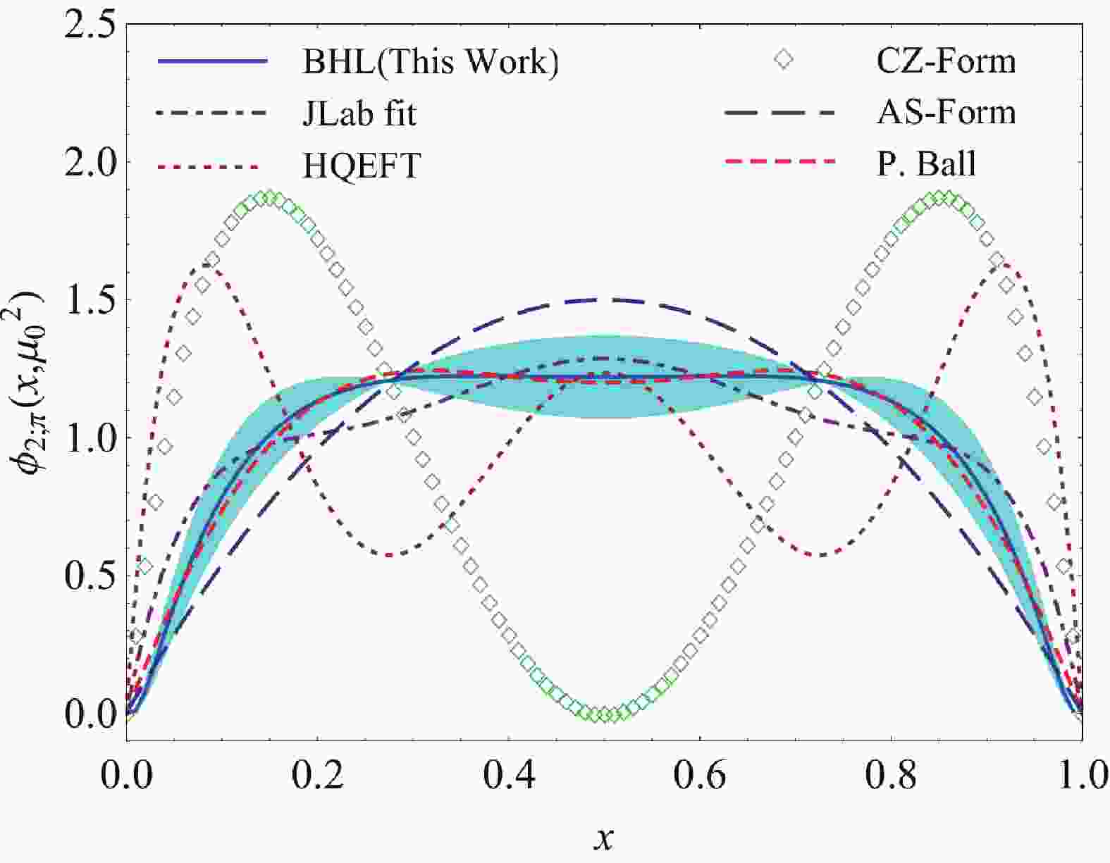
$ a_2 $ can be fixed via a global fit of the various experimental data involving pions, and we adopt the result given in Ref. [45],$a_2(\mu^2 = 1~\rm{GeV^2}) = $ $ 0.112\pm{0.073} $ . The parameters at the scale of$ 1~\rm{GeV} $ are given in Table 1, and one can get their values at any other scale by using the renormalization group evolution. At present, there is no definite conclusion whether pion LCDA$ \phi_{2;\pi}(u,\mu_0^2) $ is of the CZ form [46], asymptotic form [47], or even flat-like [48]. We present twist-2 DAs in Fig. 1, where the asymptotic form, the CZ form, the QCD SVZ sum rule prediction [18], and the prediction by A. Khodjamirian et al. [13] using the Jefferson Lab data for$ F_\pi $ , are presented for comparison. By varying$ a_2 $ , the$ \phi_{2;\pi} $ shape varies from a single-peak to double-humped behavior. The adopted BHL model provides a convenient way to mimic the pion twist-2 LCDA behavior, and we use it, together with its errors, to discuss the theoretical uncertainties related to the different choices of$ \phi_{2;\pi} $ .$a_2(\mu^2_0)$ 

A β B 0.039 23.50 0.61 0.075 0.112 24.63 0.59 0.010 0.185 23.50 0.63 0.141 Table 1. Parameters of twist-2 LCDA
$\phi _{2;\pi}(u,\mu_0^2)$ determined from$a_2(\mu^2_0)=0.112\pm{0.073}$ [45]. -
The allowed range of the Borel parameter T for
$ B \to \pi $ TFFs$ f^{+/0}(q^2) $ and the effective continuous threshold$ s_0 $ are determined from the following three conditions:● The continuum contribution should not be higher than 35% of the total LCSR;
● The contribution of all high-twist LCDAs should not exceed 50% of the total LCSR;
●The derivatives of LCSRs for TFFs with respect to
$ (-1/T) $ give LCSR for the B meson mass$ m_B $ . We require that the estimated B meson mass compared with the experimental value,$ |m^{\rm th}_B-m^{\rm exp}_B|/m^{\rm exp}_B $ , should be less than 0.1%.The flatness of TFFs with respect to the Borel parameter T provides an extra weak constraint for the range of T. With these criteria for LCSRs, the continuum threshold
$ s_0 $ and the Borel parameter T for$ B \to \pi $ vector TFF$ f^+(q^2) $ are determined as$ s_0 = 2.0\pm{0.1}\;{\rm GeV}^2 $ and$ T = 1.4\pm{0.1}\; {\rm GeV}^{2} $ for LCSR-$ \cal{R} $ , and$ s_0 = 2.2\pm{0.1}\;{\rm GeV}^2 $ and$ T = 1.5\pm{0.1}\;{\rm GeV}^2 $ for LCSR-$ \cal{U} $ .In Table 2, we show how TFF errors are related to the uncertainties of the factorization scale
$ \mu $ , the Borel parameter T, the continuum threshold$ s_0 $ , the b quark mass$ m_b $ , the B meson effective decay constant F, and twist-2 LCDA. Table 2 shows that the main errors come from the choice of$ m_b $ , F and LCDA, whose effect can be up to ~12%. Since$ m_b $ and F are correlated, e.g. a larger$ m_b $ results in a smaller F [32], we changed their values simultaneously to see the effect on TFFs.Total $\Delta \mu$ 

$\Delta DA$ 

$\Delta T$ 

$\Delta s_0$ 

$\Delta(m_b;F)$ 

$f_{\mathcal{R}}^+(0)$ 

$0.276^{+0.022}_{-0.026}$ 

$^{+0.000}_{-0.001}$ 

$^{+0.017}_{-0.016}$ 

$^{+0.001}_{-0.001}$ 

$^{+0.011}_{-0.011}$ 

$^{+0.015}_{-0.011}$ 

$f_{\mathcal{U}}^+(0)$ 

$0.282^{+0.016}_{-0.020}$ 

$^{+0.000}_{-0.000}$ 

$^{+0.009}_{-0.008}$ 

$^{+0.002}_{-0.001}$ 

$^{+0.007}_{-0.007}$ 

$^{+0.017}_{-0.012}$ 

Table 2. Uncertainties of TFFs
$f_{\mathcal{R/U}}^+(q^2)$ at$q^2 = 0$ . The uncertainties of the total TFFs are summed up in quadrature.We present the contributions of the different twist terms to the dominant
$ B \to \pi $ TFFs$ f_{\cal{R/U}}^+ $ for large recoils$ q^2 \simeq 0 \; \rm{GeV^2} $ in Table 3. In the case of the usual correlator$ F^{\cal U}_\mu $ , the contributions of the twist-3 terms are about 45% of TFF$ f_{\cal{U}}^+(0) $ . Twist-3 DAs are not as well known as DAs of twist-2. Table 3 shows that the twist-2 and twist-3 terms have similar values for the U correlator. Thus, by using the R correlator, a much better accuracy can be obtained for LCSR of the transition form factor. Table 2 shows that the errors of the U correlator are comparatively smaller, which is due to the fact that we do not include the uncertainty of twist-3 DAs in the present prediction (they are not the focus of this study). By using the chiral current correlator, we can get information about the precision of twist-2 DAs, since they can be determined exactly from the experimental data. It should be noted that it is hard to distinguish twist-2 and twist-3 with the usual current, because their contributions are almost of the same order and blend with each other. In the case of the right-handed chiral correlator$ F^{\cal R}_\mu $ , the contributions of the twist-3 terms are eliminated. Moreover, the twist-4 terms are negligible in both cases. Thus, by taking the chiral correlator, the uncertainties from higher-twist LCDAs are greatly suppressed, leading to a more precise LCSR prediction. By summing the contributions from various twist terms, the total TFFs for both correlators agree with each other within the errors①. The LCSR approximation should not depend on the choice of the chiral correlator, and our present TFF predictions provide such an example.Twist-2 Twist-3 Twist-4 Central $f_{\mathcal{R}}^+(0)$ 

0.284 − −0.009 0.276 $f_{\mathcal{U}}^+(0)$ 

0.153 0.134 −0.004 0.282 Table 3. Different twist terms in
$B \to \pi$ TFFs$f_{\mathcal{R/U}}^+$ for large recoils$q^2 \simeq 0 ~\rm{GeV^2}.$ The LCSR prediction is valid when the final-state pion has a large energy in the rest frame of B meson, e.g.
$ E_{\pi} \gg \Lambda_{\rm{QCD}} $ . Using the relation$ q^2 = m^2_B-2m_B E_{\pi} $ , we adopt a conservative range,$ 0< q^2 < 12\; \rm{GeV^2} $ , as the range of application of the LCSR method. Thus, before dealing with the$ B\to\pi $ semi-leptonic decay, we use the z-series parametrization to extrapolate the calculated TFFs to the physically allowed$ q^{2} $ region [13],$ \begin{split} f^+ \left(q^2\right) =& \displaystyle\frac{f^+ (0)}{1 - q^2/m_{B^*}^2}\bigg\{ 1 + \displaystyle\sum\limits_{k = 1}^{N - 1} b_k \bigg[z(q^2)^k - z(0)^k\\ &- ( - 1)^{N - k}\frac{k}{N}\left(z\left(q^2\right)^N - z(0)^N\right)\bigg]\bigg\} \end{split} $

(18) and
$ f^0\left(q^2\right) = f^0(0)\bigg\{ 1 + \sum\limits_{k = 1}^{N - 1} b_k (z\left(q^2\right)^k - z(0)^k)\bigg\}. $

(19) The function
$ z(q^2) $ is defined as$ z\left(q^2\right) = \frac{\sqrt {t_ + - q^2} - \sqrt {t_ + - t_0} }{\sqrt {t_ + - q^2} + \sqrt {t_ + - t_0} }, $

(20) where
$ t_ \pm = (m_B \pm m_\pi)^2 $ and$ t_0 = t_ + (1 - \sqrt {1-t_+/t_-} ) $ . The coefficients$ b_0 = f^+(0) $ ,$ b_1 $ ,$ b_2 $ and$ b_3 $ are determined such that the quality of fit$ (\Delta) $ is less than 1%. The quality of fit is defined as:$ \Delta = \frac{\sum_t {|f^{i} - f^{\rm fit}|}}{\sum_t {|f^{i}|} } \times 100 {\text{%}},\;t \in \bigg\{ 0,\frac{1}{2},...,\frac{23}{2},12\bigg\} \; \rm{GeV}^2.$

The parameters for the z-series and the quality of fit are listed in Table 4.
$b_1$ 

$b_2$ 

$b_3$ 

$\Delta$ 

$f_{\cal{R}}^+(q^2)$ 

−1.600 −1.453 − 0.03% $f_{\cal{R}}^0(q^2)$ 

−1.155 2.075 −3.377 0.01% $f_{\cal{U}}^+(q^2)$ 

−1.309 −1.757 − 0.50% $f_{\cal{U}}^0(q^2)$ 

−1.197 0.656 −0.611 0.06% Table 4. The fit parameters and quality of fit of LCSR-
$\cal{R}$ and LCSR-$\cal{U}$ TFFs$f^{+/0}(q^2) .$ The extrapolated HQEFT LCSRs for
$ B \to \pi $ TFFs$ f^{+/0}(q^2) $ are presented in Fig. 2, where the left/right plots stands for LCSR-$ {\cal R} $ /$ {\cal U} $ . The solid lines in Fig. 2 are TFFs where all parameters have their central values, while the shaded bands are TFF errors expressed as the squared average of errors from all sources. Our predictions for$ f^{+/0}(q^2) $ are consistent, within the errors, with the lattice QCD results obtained by the HPQCD and Fermilab/MILC collaborations.
Figure 2. (color online) The extrapolated
$ B\to\pi $ TFFs$ f^{+/0}(q^2) $ calculated using the two correlators LCSR-$ {\cal R} $ /$ {\cal U} $ (left/right plots). The shaded bands are the uncertainties from the error sources. As a comparison, the predictions of lattice QCD [7], LCSR [14, 15], pQCD [49] and HPQCD [50] are also shown.We adopt the correlation coefficient
$ \rho_{XY} $ to measure the degree of correlation of TFFs with different chiral correlators, defined as [40],$ \rho_{XY} = \frac{{\rm Cov}(X,Y)}{\sigma_{X}\sigma_{Y}}, $

(21) where X and Y stand for LCSR-
$ \cal{R} $ and LCSR-$ \cal{U} $ TFFs. The covariance is$ {\rm Cov}(X,Y) = E[( X-E(X)(Y-E(Y))] =$ $ E(XY)-E(X)E(Y) $ , where E is the expectation value of X or Y.$ \sigma_{X} $ and$ \sigma_{Y} $ are the standard deviations of X and Y. The range of the correlation coefficient$ |\rho_{XY}| $ is$ 0 \sim 1 $ . A larger$ |\rho_{XY}| $ indicates a higher consistency between X and Y. The correlation coefficient$ |\rho_{RU}| $ of LCSR-$ \cal{R} $ and LCSR-$ \cal{U} $ is 0.85 for the vector TFF$ f^+(q^2) $ , and 0.52 for the scalar TFF$ f^0(q^2) $ . The correlation coefficients of both TFFs are lager than 0.5, implying that they are consistent with each other. -
The
$ B \to \pi \ell\bar \nu_\ell $ differential decay widths can be written as [51, 52],$ \begin{array}{l} \displaystyle\frac{{\rm d}\Gamma(B \to \pi \ell\bar \nu_\ell )}{{\rm d}q^2} = \displaystyle\frac{G_F^2|V_{ub}|^2}{192 \pi^3 m_B^3}\frac{q^2-m_\ell^2}{(q^2)^2}\sqrt{\frac{\left (q^2-m_\ell^2 \right )^2}{q^2}} \times \sqrt{\frac{\left (m_B^2-m_\pi^2-q^2 \right )^2}{4q^2}-m_\pi^2}\Bigl \{ \left (m_\ell^2+2q^2 \right )\\ \times \left [q^2-\left (m_B-m_\pi \right )^2 \right ]\left [ q^2-\left (m_B+m_\pi \right )^2 \right ] \times f_+^2(q^2) + 3m_\ell^2\left (m_B^2-m_\pi^2 \right )^2 f_0^2(q^2)\Bigr \}, \end{array} $ 
(22) where
$ m_l $ is the lepton mass. For the light leptons$ l = e $ or$ \mu $ , the lepton mass can be safely neglected, and the differential decay width reduces to [51, 52],$ \frac{{\rm d}\Gamma(B \to \pi \ell\bar \nu_\ell )}{{\rm d}q^2} = \frac{G_F^2 |V_{ub}|^2}{ 192 \pi^3 m_B^3}\,\lambda^{3/2}(q^2) |f_+(q^2)|^2 , $

(23) where
$ |V_{ub}| $ is the CKM matrix element,$ G_F $ is the Fermi coupling constant, and the phase-space factor is$ \lambda(q^2) = (m_B^2+m_\pi^2-q^2)^2 - 4 m_B^2 m_\pi^2 $ . The branching fraction is related to the decay width as${\rm d}{\cal B}/{\rm d}q^2 = {\rm d}\Gamma (B \to \pi \ell\bar \nu_\ell)/$ $ {\rm d}q^2\times \tau_{B^0} $ , where the total lifetime is$\tau_{B^0} = $ $ 1.525\pm{0.009} $ ps [40]. Fig. 3 shows that both LCSR-$ {\mathcal R} $ and LCSR-$ {\mathcal U} $ predictions, including their errors (shown by shaded bands), are consistent with the BABAR and BELLE data.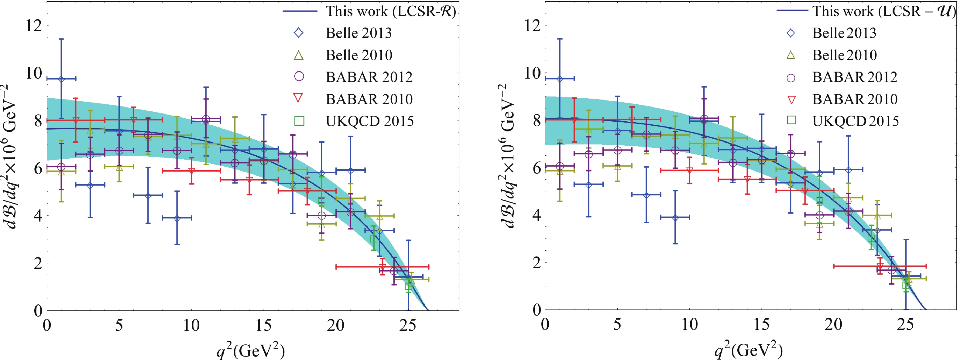
The integrated branching fraction was experimentally measured as
$ \Delta {\cal B}(0,q_f^2) = \int_{0}^{q_f^2} ({\rm d}{\cal B}/{\rm d}q^2) {\rm d}q^2 $ [53, 54],$ \begin{split} \Delta {\cal B}(0,12\rm{GeV}^2) = & (0.83 \pm 0.03 \pm 0.04) \times 10^{ - 4},\\ &({\rm BABAR}\; 2012) \end{split} $

(24) $ \begin{split} \Delta {\cal B}(0,12\rm{GeV}^2) = &(0.808 \pm 0.06) \times 10^{ - 4}.\\ & ({\rm Belle}\; 2013) \end{split} $

(25) Using their weighted average, we can determine the value of
$ |V_{ub}| $ $ \begin{array}{l} |V_{ub}|_{\cal R} = (3.45^{+0.28}_{-0.20}\pm{0.13}_{\rm{exp}})\times10^{-3}, \end{array} $

(26) $ \begin{array}{l} |V_{ub}|_{\cal U} = (3.38^{+0.22}_{-0.16}\pm{0.12}_{\rm{exp}})\times10^{-3}, \end{array} $

(27) where the first error is the squared average of the input parameter errors, and the second is the experimental error of
$ \Delta {\cal B}(0,12\rm{GeV}^2) $ .A comparison of
$ |V_{ub}| $ using various approaches is presented in Table 5. Most predictions are consistent with each other within errors. Our HQEFT LCSR predictions show good agreement with the Belle measurements [54], as well as the usual LCSR predictions [13, 15].Exclusive decays $B\rightarrow \pi\ell \bar{\nu}_{\ell} $ 

$|V_{ub}|\times 10^{3}$ 

LCSR- $\cal{R}$ (This work)

$3.45{^{+0.28}_{-0.20}\pm{0.13}_{\rm{exp}}}$ 

LCSR- $\cal{U}$ (This work)

$3.38{^{+0.22}_{-0.16}\pm{0.12}_{\rm{exp}}}$ 

RBC/UKQCD [7] $3.61\pm0.32$ 

Fermilab/MILC [8] $3.72\pm0.16$ 

pQCD [9] $3.80{^{+0.56}_{-0.50}}$ 

$B$ -meson LCSR [13]

$3.50{^{+0.38}_{-0.33}\pm{0.11}_{\rm{exp}}}$ 

Imsong 2014 (LCSR) [15] $3.32{^{+0.26}_{-0.22}}$ 

BABAR 2012 [53] $3.25\pm0.31$ 

Belle 2013 [54] $3.52\pm0.29$ 

CKM fitter [57] $3.71{^{+0.24}_{-0.19}}$ 

UT fitter [58] $3.68\pm{0.10}$ 

FLAG 2016 [59] $3.62\pm0.14$ 

HFAG 2016 [60] $3.67\pm0.21$ 

Table 5. A comparison of
$|V_{ub}|$ derived using various approaches.The correlation coefficient for the branching fractions obtained with LCSR-
$ {\mathcal R} $ and LCSR-$ {\mathcal U} $ TFFs is$ \rho_{\rm RU} = 0.85 $ , which confirms the previous observation that the physical observable should be independent of the choice of correlator. In Table 6 , a comparison is given of the above branching fractions of$ B\to \pi \ell \bar \nu_\ell $ with the experimental measurements, which shows that both LCSR-$ \cal{U} $ and LCSR-$ \cal{R} $ predictions are consistent with the data.Exclusive decays $B\rightarrow \pi\ell \bar{\nu}_{\ell} $ 

${\cal B}\times10^{4}$ 

LCSR- $\cal{R}$ (This work)

$1.41{^{+0.30}_{-0.26}}$ 

LCSR- $\cal{U}$ (This work)

$1.39{^{+0.24}_{-0.21}}$ 

PDG [40] $1.50\pm{0.06}$ 

BABAR 2012 [53] $1.44{\pm0.04}{\pm0.06}$ 

Belle 2013 [54] $1.49{\pm0.09}{\pm0.07}$ 

BABAR 2010 [55] $1.41{\pm0.05}{\pm0.08}$ 

Belle 2010 [56] $1.49{\pm0.04}{\pm0.07}$ 

CLEO [61] $1.38{\pm0.15}{\pm0.11}$ 

HFAG 2016 [60] $1.50{\pm0.02}{\pm0.04}$ 

Table 6. A comparison of the branching fraction of
$B\to \pi \ell \bar \nu_\ell$ with the experimental measurements. Both LCSR-$\cal{U}$ and LCSR-$\cal{R}$ predictions are consistent with the data.As a final remark, it is more useful to measure the following ratio, which avoids uncertainties from the input parameters such as
$ |V_{ub}| $ and could be used as a precision test of SM or to find new physics beyond SM,$ \begin{split} \cal{R}_{\pi} \equiv &\displaystyle\frac{{\cal{B}}(B\to \pi \tau \bar{\nu_\tau})}{{\cal{B}}(B\to \pi \ell \bar{\nu_\ell})} =\displaystyle \frac{\displaystyle\int^{q^2_{\max}}_{m^2_{\tau}}{\rm d}\Gamma(B\to \pi \tau \bar{\nu_{\tau}})/{\rm d}q^2}{\displaystyle\int^{q^2_{\max}}_{0}{\rm d}\Gamma (B\to\pi \ell \bar{\nu_\ell})/{\rm d}q^2}. \end{split} $

(28) This ratio strongly depends on the behavior of
$ B\to\pi $ TFFs. Briefly, due to the phase-space suppression, the decay width of$ B\to \pi \tau \bar{\nu_\tau} $ is smaller than of$ B\to\pi \ell \bar{\nu_\ell} $ , leading to$ \cal{R}_{\pi}<1 $ in SM. The RBC and UKQCD collaborations predicted$ R_{\pi} = 0.69\pm{0.19} $ , using the lattice QCD calculations for$ B\to\pi $ TFFs [7]. By using the LCSR-$ {\mathcal R} $ and LCSR-$ {\mathcal U} $ predictions for TFFs, we obtain$ {\cal{R}}_{\pi}^{\cal{R}} = 0.65^{+0.13}_{-0.11}, \quad {\cal{R}}_{\pi}^{{\cal{U}}} = 0.68^{+0.10}_{-0.09}. $

(29) Both values agree with the lattice QCD prediction. However, the Belle measurements lead to a rather large ratio [5],
${R}^{\rm{exp}}_{\pi}\simeq1.05\pm{0.51} $ . A way out is to increase the magnitude of the chiral symmetry breaking terms which are proportional to$ f_0^2(q^2) $ . For example, by using the type-II two Higgs doublet model (2HDM), one obtains [6],$ \begin{array}{l} f_0^{\rm 2HDM}(q^2) \approx f_0^{\rm SM}(q^2) \left(1 - \displaystyle\frac{\tan ^2 \beta }{m_{H^ \pm }^2}\displaystyle\frac{q^2}{1 - m_u/m_b}\right) \end{array}, $

(30) where the parameter
$ \tan \beta $ is the ratio of the two vacuum expectations of the Higgs doublets, and$ m_{H^{\pm}} $ is the mass of the charged Higgs. By setting$ \tan \beta/m_{H^+} = 0.4 $ [6], we obtain${R}_{\pi}^{\rm 2HDM;\cal{R}} = 0.95 ^{+0.08}_{-0.09} $ and${R}_{\pi}^{\rm 2HDM;\cal{U}} = 1.02 ^{+0.01}_{-0.06} $ . In Ref. [62], the latest CMS results at$ \sqrt{s} = 13 $ TeV were used to impose a constraint on the charged Higgs$ H^{\pm} $ parameters in 2HDM, but some parameters are still not fully determined. Thus, we get the same result as Ref. [6], indicating that there may be new physics beyond SM. However since the Belle measurements have large errors, we still need more measurements to confirm whether thus is really the case. -
In this paper, we have made a detailed LCSR analysis of
$ B \to \pi \ell \bar\nu_\ell $ TFFs in the framework of HQEFT. As shown in Fig. 2, LCSR-$ \cal{U} $ and LCSR-$ \cal{R} $ , obtained using two different correlators, are highly correlated with$ \rho_{RU} > 0.5 $ , especially for$ f^+(q^2) $ , which provides a dominant contribution to the$ B\to\pi $ semileptonic decays. The LCSR method is applicable in the low and intermediate$ q^2 $ regions and the lattice QCD method in the large$ q^2 $ region. After extrapolation, our HQEFT LCSR predictions for TFFs agree well with the lattice QCD predictions obtained by the HPQCD and Fermilab/MILC collaborations. As a byproduct, by using the chiral correlator, it was shown that twist-2 LCDA contributes to more than 97% of TFFs, and thus is a good platform for testing the properties of pion twist-2 LCDA. Moreover, by using LCSR-$ \cal{U} $ and LCSR-$ \cal{R} $ TFFs, we obtain,$ |V_{ub}|_{\cal R} = (3.45^{+0.28}_{-0.20}\pm $ ${0.13}_{\rm{exp}})\times10^{-3} $ and$|V_{ub}|_{\cal U} = $ $ (3.38^{+0.22}_{-0.16}\pm{0.12}_{\rm{exp}})\times10^{-3} $ , both of which are in agreement with the experimental results within errors. The ratio$ \cal{R}_{\pi} $ is a useful parameter to test SM, and to provide indication of new physics beyond SM.We are grateful to Tao Zhong and Jun Zeng for helpful discussions.
-
The relations between pion LCDAs up to twist-
$4 $ and the nonlocal matrix elements are:$\tag{A1} \begin{array}{l} \langle \pi(p) |\bar u(x) \gamma_\mu \gamma_5 d(0)|0 \rangle = - i p_\mu f_\pi \displaystyle\int_0^1 {\rm d}u {\rm e}^{{\rm i}up\cdot x} [ \phi_{2;\pi} (u) \\ \qquad + x^2 g_1(u) ] + f_\pi \bigg(x_\mu - \displaystyle\frac{x^2 p_\mu }{p\cdot x}\bigg)\int_0^1 {\rm d}u {\rm e}^{ -{\rm i}up\cdot x} g_2 (u),\\ \end{array} $

$\tag{A2} \begin{array}{l} \langle \pi (p) |\bar u(x)i \gamma_5 d(0) |0\rangle = \displaystyle\frac{f_\pi m_\pi^2}{m_u + m_d}\int_0^1 {{\rm d}u{{\rm e}^{{\rm i}up \cdot x}}} {\phi_{3;\pi}^p(u)},\\ \end{array} $

$\tag{A3} \begin{split} \langle \pi (p)|\bar u(x) \sigma_{\mu \nu}\gamma_5 d(0)| \rangle =& i(p_\mu x_v - p_v x_\mu)\frac{f_\pi m_\pi^2}{6(m_u + m_d)} \\ &\times\int_0^1 {\rm d}u {\rm e}^{{\rm i}up \cdot x} \phi _{3; \pi}^\sigma(u). \end{split} $

Here,
$ f_\pi $ is the pion decay constant, and$ \phi_{2;\pi}(u) $ ,$ \phi_{3;\pi}^p(u) $ ,$ \phi _{3; \pi}^\sigma(u) $ ,$ g_1(u) $ and$ g_2(u) $ are pion twist-2, 3 and 4 LCDAs, respectively. Twist-3 LCDAs take the form$\tag{A4} \begin{split} {\phi _{3;\pi }^p(u)} = &{1 + \frac{1}{2}{B_2}(3{\xi ^2} - 1) + \frac{1}{8}{B_4}(35{\xi ^4} - 30{\xi ^2} + 3),} \\ \phi _{3;\pi }^\sigma (u) = &6u\bar u \Big[1 + \frac{3}{2}{C_2}(5{\xi ^2} - 1) \hfill \\ & + \frac{{15}}{8}{C_4}(21{\xi ^4} - 14{\xi ^2} + 1)\Big], \hfill \\ \end{split}$

where the parameters are [26, 27, 63, 64],
$ B_2(\mu _b) = 0.29 $ ,$ B_4(\mu _b) = 0.58 $ ,$ C_2(\mu _b) = 0.059 $ and$ C_4(\mu _b) = 0.034 $ . For twist-4 LCDAs, we adopt the expressions derived in Ref. [39],$\tag{A5} \begin{split} {{g_1}(u)} =& {\frac{{\bar uu}}{6}[ - 5\bar uu(9{h_{00}} + 3{h_{01}} - 6{h_{10}} + 4\bar u{h_{01}}u } \\ & { + 10\bar u {h_{10}}u) + {a_{10}}(6 + \bar uu(9 + 80\bar uu))] + {a_{10}}{{\bar u}^3}(10} \\ & { - 15\bar u + 6{{\bar u}^2})\ln \bar u + {a_{10}}{u^3}(10 - 15u + 6{u^2})\ln u,} \\ {g_2}(u) =& \frac{{5\bar uu(u - \bar u)}}{2}[4{h_{00}} + 8{a_{10}}\bar uu \hfill \\ & - {h_{10}}(1 + 5\bar uu) + 2{h_{01}}(1 - \bar uu)], \end{split} $

where
$ \begin{array}{l} h_{00} = -\displaystyle\frac{\delta^2}{3}, \; a_{10} = \delta^2\epsilon-\displaystyle\frac{9}{20} a^\pi_2 m_\pi^2,\\ h_{01} = \displaystyle\frac{2}{3}\delta^2\epsilon-\displaystyle\frac{3}{20} a^\pi_2 m_\pi^2, \; v_{10} = \delta^2\epsilon , \\ h_{10} = \displaystyle\frac{4}{3}\delta^2\epsilon+\displaystyle\frac{3}{20} a_2^\pi m_\pi^2 . \end{array} $

where
$ \epsilon (\mu _b) = 0.36 $ , and$ \delta ^2(\mu _b) = 0.17\;\rm{GeV}^2 $ [26, 27].
The ${{B\to \pi \ell\nu_\ell}}$ semileptonic decay within the LCSR approach under heavy quark effective field theory
- Received Date: 2019-10-08
- Available Online: 2020-01-01
Abstract: The heavy quark effective field theory (HQEFT) provides an effective way to deal with heavy meson decays. In this paper, we adopt two different correlators to derive the light-cone sum rules (LCSR) for the


 DownLoad: