


 Abstract
 HTML
HTML Reference
 Related
 PDF
PDF


-
After the discovery of the Higgs boson at the Large Hadron Collider (LHC) [1–4], the outstanding task is to learn about its properties and confirm them either experimentally or theoretically. Among its various decay modes, the Higgs decay into two photons,
$ H\to\gamma\gamma $ , which can be observed at the LHC or a high luminosity$ e^+ e^- $ linear collider, provides a clean platform for studying the Higgs properties and for testing the Standard Model.The Higgs boson couples dominantly to the massive particles and the leading order (LO) term of the total decay width
$ \Gamma(H\to\gamma\gamma) $ is already at the one-loop level, which conversely makes the high-order pQCD corrections very complicated. The LO, the next-to-leading order (NLO), the N2LO, the approximate N3LO and the N4LO terms for the total decay width$ \Gamma(H\to\gamma\gamma) $ were calculated in Refs. [5–18]. In particular, the fermionic contributions, which form a gauge invariant subset, were given in the N3LO and N4LO terms [18]. As shall be shown below, these state-of-art terms give the opportunity to achieve a more precise prediction of$ \Gamma(H\to\gamma\gamma) $ . Due to the complexity of high-order pQCD calculations, it is important to use the known fixed-order terms to obtain the perturbative properties as accurately as possible.Following the standard renormalization group invariance, a pQCD calculable physical observable, corresponding to an infinite order prediction, should be independent of the choice of renormalization scheme and renormalization scale. However, for a fixed-order approximant, one needs to set an optimal scale for comparison with the data. Conventionally, the renormalization scale is chosen as the typical momentum flow of the process, or such to eliminate the large log terms. In this simple treatment, the running coupling and its coefficients of the same order cannot be exactly matched, leading to the well-known renormalization scheme-and-scale ambiguities. Due to these ambiguities, the renormalization scale uncertainty is always treated as the key error of a theoretical prediction, which is assumed to decrease when more loop terms are included. As an example, Ref. [18] showed that when going from LO to the approximate N4LO, the scale dependence of the total decay width
$ \Gamma(H\to\gamma\gamma) $ decreases continuously with increasing number of loop terms. However, such a decreasing scale dependence is caused by compensation of scale dependence among different orders, and the exact value for each loop term cannot be obtained by using the “guessing” scale. There are many other problems for such conventional scale-setting treatment [19, 20]. It is thus important to find a proper scale-setting approach to set the renormalization scale so as to achieve a more accurate fixed-order prediction.The principle of maximum conformality (PMC) [21–25] has been suggested for eliminating the renormalization scheme-and-scale ambiguities. The key idea is to set the correct momentum flow of the process, whose value is independent of the choice of the renormalization scale, based on the renormalization group equation (RGE). Its prediction thus avoids the conventional renormalization scale ambiguities. When one applies PMC, all non-conformal terms that govern the
$ \alpha_s $ running behavior of the pQCD approximant, should be systematically resummed. The PMC prediction satisfies the renormalization group invariance and all self-consistency conditions of the renormalization group [26]. PMC resums all$ \{\beta_i\} $ terms, the divergent renormalon terms which are proportional to$ n!\beta_0^n\alpha_s^n $ generally disappear, and a more convergent pQCD series can be naturally achieved. Due to the scheme independent nature of the conformal series and the commensurate scale relations among different observables [27, 28], the PMC predictions are scheme independent. In this paper we adopt PMC to set the renormalization scale for the decay width$ \Gamma(H\to\gamma\gamma) $ up to N4LO, and show that an accurate scale independent prediction can indeed be achieved. For clarity, we adopt the PMC single-scale approach (PMC-s) [29] for scale-setting. -
The total decay width of the Higgs decay into two photons at the one-loop level takes the form
$ \Gamma(H \rightarrow \gamma\gamma) = \frac{M_{\rm H}^{3}} {64\pi} \left|A_{W}+\sum\limits_{f} A_{f}\right|^{2}, $

(1) where
$ M_{\rm H} $ is the Higgs mass,$ A_W $ denotes the contribution from the purely bosonic diagrams, and$ A_f $ stands for the contribution from the amplitudes with$ f = (t, b, c, \tau) $ , which correspond to top quark, bottom quark, charm quark and$ \tau $ lepton, respectively.The higher-order N2LO, N3LO and N4LO expressions were given in Refs. [17, 18] for the top quark running mass
$ (m_t) $ . To set the correct momentum flow of the process, only those$ \{\beta_i\} $ terms that pertain to RGE should be resummed into$ \alpha_s $ . Thus, as was argued in Ref. [30], we transform these terms into the top quark pole mass$ (M_t) $ so as to avoid entanglement of the$ \{\beta_i\} $ terms from either the top quark anomalous dimension or RGE, and thus avoid the ambiguity in applying PMC. Such a mass transformation can be done by using the relation between$ m_t $ and$ M_t $ , whose explicit expression up to the$ \alpha_s^4 $ order can be found in Ref. [31].For convenience, we rewrite the total decay width in two parts,
$ \Gamma(H \rightarrow \gamma\gamma) = \frac{M_{\rm H}^{3}} {64\pi} \bigg( A_{\rm LO}^{2} + A_{\rm EW} {\alpha\over \pi}\bigg) + R(\mu_r), $

(2) where
$ \alpha $ is the fine-structure constant.The LO contribution
$ A_{\rm LO} $ and the electroweak (EW) correction$ A_{\rm EW} $ are [17]$ A_{\rm LO} = A_{W}^{(0)}+A_{f}^{(0)}+\hat A_t A_{t}^{(0)}, $

(3) $ A_{\rm EW} = 2 A_{\rm LO} A^{(1)}_{\rm EW} , $

(4) where
$ A_W^{(0)} $ is the purely bosonic contribution to the amplitude,$ A_f^{(0)} $ is the contribution to the amplitude with$ f = (b,c,\tau) $ ,$ \hat{A}_t = 2 Q_t^2 \alpha \sqrt{\sqrt{2} G_{\rm F}}/\pi $ ,$ G_{\rm F} $ is the Fermi constant, and$ Q_t $ is the top quark electric charge. All were calculated in Refs. [5, 6], i.e.$ \begin{split} A_W^{(0)} = & -\frac{\alpha\sqrt{\sqrt{2}G_{\rm F}}}{2\pi} \left[ 2+\frac{3}{\tau_W}+\frac{3}{\tau_W}\left(2-{1\over\tau_W}\right) f(\tau_W) \right], \\ A_f^{(0)} = & \sum\limits_{f = c,b,\tau} 3\frac{\alpha \sqrt{\sqrt{2} G_{\rm F}}}{\pi \tau_{f}} Q_f^2 \left[1+\bigg(1-{1\over \tau_{f}}\bigg) f(\tau_f)\right], \\ A_t^{(0)} = & 1+{7\over30} \tau_t+{2\over21} \tau_t^2+{26\over525} \tau_t^3+{512\over17325} \tau_t^4 + {1216\over63063} \tau_t^5\\& +{128\over9555} \tau_t^6, \end{split} $

where
$ f(\tau)=\left\{ \begin{array}{ll} {\rm Arcsin}^2(\sqrt{\tau}) &\quad {\rm{for}}\quad \tau\leqslant 1\\ -\displaystyle\frac{1}{4}\left[\ln\displaystyle\frac{1+\sqrt{1-\tau^{-1}}}{1-\sqrt{1-\tau^{-1}}}-i\pi\right]^2& \quad {\rm{for}}\quad \tau>1 \end{array} \right. , $

$ Q_f $ denotes the electric charge of$ f = (c,b,\tau) $ ,$ \tau_W = M^2_{\rm H}/(4M_W^2) $ ,$ \tau_t = M_{\rm H}^2/(4 M_t^2) $ and$ \tau_{f} = M^2_{\rm H}/(4 M_f^2) $ , and the expression for the NLO electroweak term$ A^{(1)}_{\rm EW} $ can be found in Refs. [31, 32].The QCD corrections of the decay width
$ \Gamma(H \to \gamma\gamma) $ are separately represented by$ R(\mu_r) $ , whose perturbative series up to the$ (n+1) $ loop level can be written as$ R_n(\mu_r) = \sum\limits_{i = 1}^{n} r_{i}(\mu) a_s^{i}(\mu_r), $

(5) where
$ a_s = {\alpha_s}/\pi $ ,$ \mu_r $ is the renormalization scale. The perturbative coefficients$ r_i $ in the$ \overline{\rm MS} $ scheme up to the$ \alpha_s^4 $ order can be derived from Refs. [17, 18]. To apply PMC, the$ n_f $ power series ($ n_f $ being the active flavor number) of the coefficients$ r_i $ should be rewritten into conformal terms and non-conformal$ \beta_i $ terms [24, 25],$ r_1 = r_{1,0}, $

(6) $ r_2 = r_{2,0} + r_{2,1} \beta_0, $

(7) $ r_3 = r_{3,0} + r_{2,1} \beta_1 + 2r_{3,1} \beta_0 + r_{3,2} \beta_0^2, $

(8) $ \begin{split} r_4 =& r_{4,0} + r_{2,1} \beta_2 + 2r_{3,1} \beta_1 + \frac{5}{2} r_{3,2} \beta_0 \beta_1 \\ & + 3r_{4,1} \beta_0 + 3r_{4,2} \beta_0^2 + r_{4,3} \beta_0^3, \\ &\cdots,\end{split} $

(9) where the
$ \beta $ pattern at each order is a superposition of RGE, and all coefficients$ r_{i,j} $ can be fixed from the$ n_f $ power series at the same order by using the degeneracy relations among different orders.$ r_{i,0} $ are conformal coefficients which are exactly free of$ \mu_r $ for the present channel, and$ r_{i,j(j\neq 0)} $ are non-conformal coefficients which are functions of$ \mu_r $ , i.e.,$ r_{i,j} = \sum\limits_{k = 0}^{j} C_j^k \ln^k(\mu_r^2/M_{\rm H}^2) \hat{r}_{i-k,j-k}, $

(10) where
$ \hat{r}_{i,j} = r_{i,j}|_{\mu_r = M_H} $ . The needed$ \{\beta_i\} $ functions in the$ \overline{\rm MS} $ scheme are given in Refs. [33–41].Following the standard procedures of the PMC single-scale approach [29], the pQCD corrections of the decay width
$ \Gamma(H \to \gamma\gamma) $ can be simplified as the following conformal series,$ R_n(\mu_r)|_{\rm PMC} = \sum\limits_{i = 1}^{n} \hat{r}_{i,0} a_s^i(Q_\star), $

(11) where
$ Q_{\star} $ is the PMC scale. Using the known pQCD corrections up to N4LO,$ Q_{\star} $ can be fixed up to next-to-next-to-leading-log (${ \rm N^2LL} $ ) accuracy, i.e.,$ \ln\frac{Q_\star^2}{M_{\rm H}^2} = \sum\limits_{i} T_{i} a^{i}_s(M_{\rm H}), $

(12) whose first three coefficients with
$ i = (0,1,2) $ can be determined from the known five-loop QCD corrections of the decay width$ \Gamma(H \to \gamma\gamma) $ , which are$ T_0 = -{\hat{r}_{2,1}\over \hat{r}_{1,0}}, $

(13) $ T_1 = {2(\hat{r}_{2,0}\hat{r}_{2,1}-\hat{r}_{1,0}\hat{r}_{3,1})\over \hat{r}_{1,0}^2} +{(\hat{r}_{2,1}^2-\hat{r}_{1,0}\hat{r}_{3,2})\over \hat{r}_{1,0}^2}\beta_0, $

(14) $ \begin{split} T_2 = &{4(\hat{r}_{1,0}\hat{r}_{2,0}\hat{r}_{3,1}-\hat{r}_{2,0}^2\hat{r}_{2,1}) +3(\hat{r}_{1,0}\hat{r}_{2,1}\hat{r}_{3,0}-\hat{r}_{1,0}^2\hat{r}_{4,1})\over \hat{r}_{1,0}^3 }\\ &-{\hat{r}_{2,0}\hat{r}_{2,1}^2 +2(\hat{r}_{2,0}\hat{r}_{2,1}^2-2\hat{r}_{1,0}\hat{r}_{2,1}\hat{r}_{3,1} -\hat{r}_{1,0}\hat{r}_{2,0}\hat{r}_{3,2})\over \hat{r}_{1,0}^3}\beta_0\\ &-{3\hat{r}_{1,0}^2\hat{r}_{4,2}\over \hat{r}_{1,0}^3}\beta_0 +{3(\hat{r}_{2,1}^2-\hat{r}_{1,0}\hat{r}_{3,2})\over 2\hat{r}_{1,0}^2}\beta_1 \\ &+{(\hat{r}_{1,0}\hat{r}_{2,1}\hat{r}_{3,2}-\hat{r}_{1,0}^2\hat{r}_{4,3})+(\hat{r}_{1,0}\hat{r}_{2,1}\hat{r}_{3,2}-\hat{r}_{2,1}^3)\over \hat{r}_{1,0}^3}\beta_0^2. \end{split} $

(15) It should be noted that all perturbative coefficients
$ T_i $ are free of$ \mu_r $ , and Eq. (12) then indicates that the PMC scale$ Q_\star $ is free of$ \mu_r $ . Together with the fact that the conformal coefficients$ \hat{r}_{i,0} $ are also free of$ \mu_r $ , the PMC approximant$ R_n(\mu_r)|_{\rm PMC} $ is exactly scale independent. Thus the conventional scale ambiguity is eliminated.As a subtle point, due to the perturbative nature of the PMC scale
$ Q_\star $ , there is a residual scale dependence of the pQCD approximant for the unknown higher-order terms in$ Q_\star $ perturbative series. However, this residual scale dependence is different from conventional renormalization scale ambiguity. In fact this residual scale dependence is usually negligible due to both the$ \alpha_s $ suppression and exponential suppression. This property has been confirmed in many PMC applications in literature. -
For numerical calculations, we take the following central values [42]: the
$ W $ boson mass$ M_{W} = 80.379 $ GeV, the$ \tau $ lepton mass$ M_{\tau} = 1.77686 $ GeV, the$ b $ quark pole mass$ M_{b} = 4.78 $ GeV, the$ c $ quark pole mass$ M_{c} = 1.67 $ GeV, the$ t $ quark pole mass$ M_{t} = 173.07 $ GeV, and the Higgs mass$ M_{H} = 125.9 $ GeV. The Fermi constant is$ G_{\rm F} = 1.1663787\times10^{-5} $ $ \rm GeV^{-2} $ and the fine-structure constant$ \alpha = 1/137.035999139 $ . The magnitude of the EW corrections at the NLO level is about 0.15 KeV [43], which shall be altered to ~0.18 KeV by setting the scale for the fine structure constant to be$ M_{\rm H}/2 $ , leading to about 20% scale uncertainty for the EW corrections. In the present paper, we shall concentrate on eliminating the scale uncertainty for QCD corrections. The PMC is applicable to QED corrections [19], and if the NNLO and higher order EW corrections are known, one can determine the correct$ \alpha $ value by using the PMC via a similar way. To be self-consistent with the N4LO pQCD correction of the total decay width$ \Gamma(H\to\gamma\gamma) $ , we adopt the four-loop$ \alpha_s $ running and$ \alpha_s(M_{Z} = 91.1876{\rm GeV}) = 0.1181 $ to fix the$ \alpha_{s} $ running behavior.As a comparison, we present the total decay width
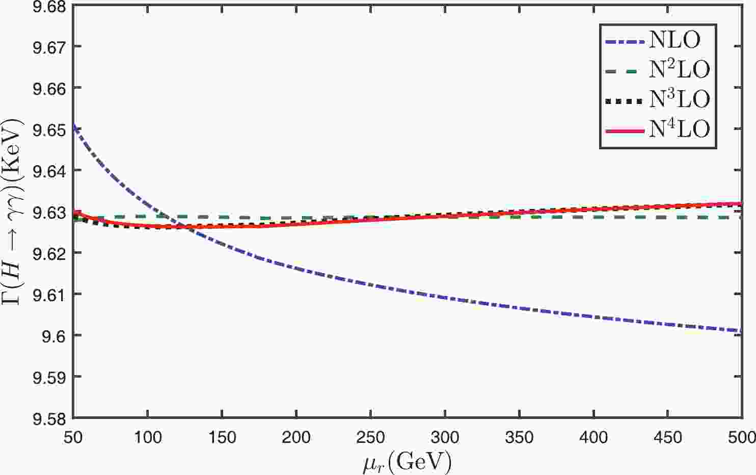
$ \Gamma(H\to\gamma\gamma) $ up to N4LO with the conventional and PMC scale-settings in Figs. 1 and 2. In agreement with previous observations, Fig. 1 shows that with the conventional scale-setting the scale dependence becomes smaller and smaller when more loop terms are included. The N4LO total decay width in the conventional scale-setting gives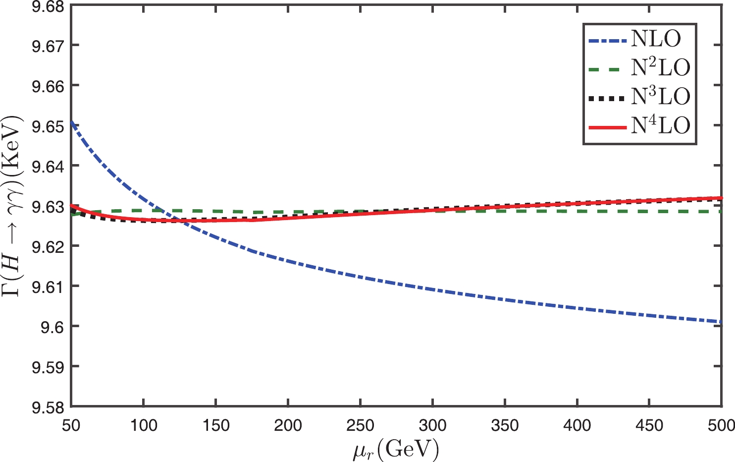
Figure 1. (color online) Total decay width
$ \Gamma(H\to\gamma\gamma) $ versus the initial scale$ \mu_r $ up to N4LO with the conventional scale-setting.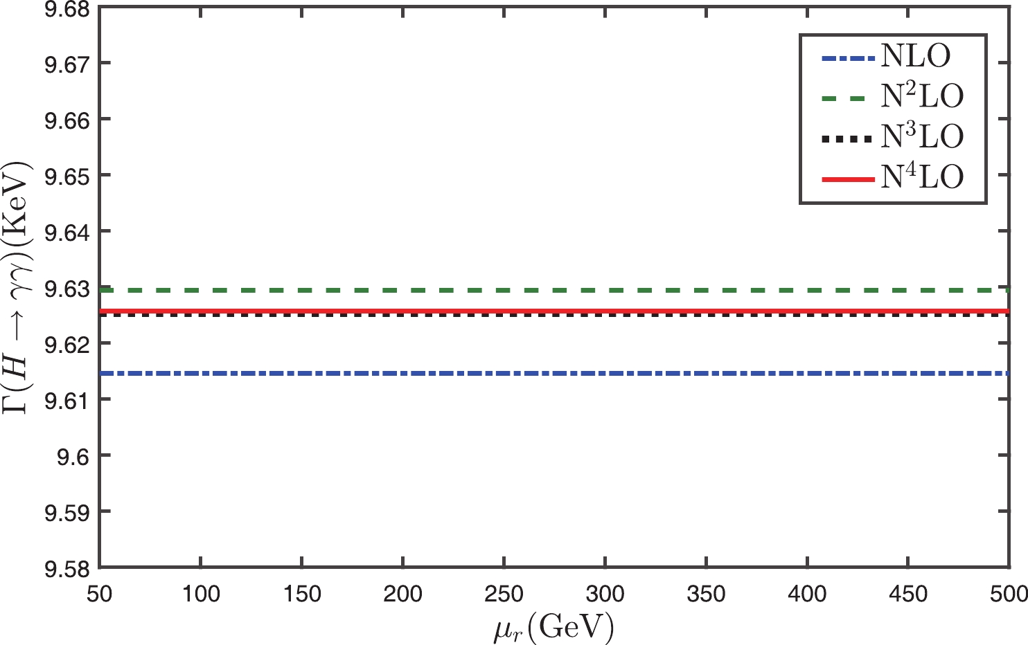
Figure 2. (color online) Total decay width
$ \Gamma(H\to\gamma\gamma) $ versus the initial scale$ \mu_r $ up to N4LO with the PMC scale-setting.$ \Gamma(H\to\gamma\gamma)|_{\rm Conv.} = 9.626^{+0.002}_{+0.002}\; {\rm KeV}, $

(16) where the central value is for
$ \mu_r = M_{\rm H} $ , and the renormalization scale error is for$ \mu_r\in[M_{\rm H}/2, 2M_{\rm H}] $ .It should be pointed out that the above approximate scale independence of the N4LO total decay width
$ \Gamma(H\to\gamma\gamma) $ with the conventional scale-setting is caused by large cancellations of the scale dependence among different orders. This can be explicitly seen in Table 1, in which the individual decay widths for LO+EW, NLO, N2LO, N3LO and N4LO are presented separately. More explicitly, we define a parameter$ \kappa_i $ to measure the scale dependence of the separate decay widths at different orders, i.e.$i={\rm LO+EW}$ 

$i={\rm NLO}$ 

$i={\rm N^2LO}$ 

${\rm N^3LO}$ 

$i={\rm N^4LO}$ 

total ${\Gamma_i \rm{(KeV)}}|_{\rm Conv.}$ 

$\mu_r=M_{\rm H}/2$ 

9.46477 0.17927 −0.01573 −0.00085 0.00083 9.62830 $\mu_r=M_{\rm H}$ 

9.46477 0.16133 0.00263 −0.00242 −0.00007 9.62624 $\mu_r=2M_{\rm H}$ 

9.46477 0.14731 0.01649 −0.00038 −0.00028 9.62791 ${\Gamma_i\rm{(KeV)}}|_{\rm PMC}$ 

$\mu_r\in[M_{\rm H}/2,2M_{\rm H}]$ 

9.46477 0.14979 0.01489 −0.00423 0.00056 9.62578 Table 1. Total decay width
$ \Gamma(H\to\gamma\gamma) $ with the conventional (Conv.) and PMC scale-settings.$ \Gamma_{\rm LO+EW} $ ,$ \Gamma_{\rm NLO} $ ,$ \Gamma_{\rm N^{2}LO} $ ,$ \Gamma_{\rm N^{3}LO} $ and$ \Gamma_{\rm N^{4}LO} $ are individual decay widths for LO+EW, NLO,$ {\rm N}^{2} $ LO,$ {\rm N}^{3} $ LO and$ {\rm N}^{4} $ LO, respectively. The final row is the total decay width up to$ {\rm N}^{4} $ LO. Three typical scales$ \mu_{r} $ =$ M_{\rm H}/2 $ ,$ M_{\rm H} $ ,$ 2 M_{\rm H} $ are adopted.$ \kappa_i = \frac{\left. \Gamma_{i}\right|_{\mu_{r} = M_{\rm H}/2} -\left. \Gamma_{i}\right|_{\mu_{r} = 2M_{\rm H}}}{\left. \Gamma_{i} \right|_{\mu_{r} = M_{\rm H}}}, $

(17) where the subscript
$ i $ stands for the individual NLO, N2LO, N3LO and N4LO decay widths. In the conventional scale-setting, we have$ \kappa_{\rm NLO} = +20\text{%}, $

(18) $ \kappa_{\rm {N^2LO}} = -1.2\times10^3\text{%}, $

(19) $ \kappa_{\rm {N^3LO}} = +19\text{%}, $

(20) $ \kappa_{\rm {N^4LO}} = -1.6\times10^3\text{%}. $

(21) Large magnitude of
$ \kappa_i $ indicates that in the conventional scale-setting, there are large scale errors for each order. Due to the cancellation among different orders, the net scale error for the N4LO total decay width is small and is about 0.2%.On the other hand, as shown in Fig. 2, the PMC prediction is almost scale independent for each order, and the PMC prediction of
$ \Gamma(H\to\gamma\gamma) $ quickly approaches the scale independent “physical” value due to a faster convergence than the conventional pQCD series. As the magnitudes of the newly added N3LO and N4LO terms are only about 28% and 4% of the N2LO term, whose magnitude is small, our previous N2LO PMC prediction agrees with the present one [44] to a high precision. Table 1 shows that after applying PMC, both the separate decay widths and the total decay width are unchanged for$ \mu_r\in[M_{\rm H}/2, 2M_{\rm H}] $ . The N4LO total decay width with the PMC scale-setting is$ \Gamma(H\to\gamma\gamma)|_{\rm PMC} \equiv 9.626\; {\rm KeV}. $

(22) The four-loop and five-loop fermionic contributions are helpful to set an accurate PMC scale. The effective scale
$ Q_\star $ can be fixed up to the$ {\rm N^{2}LL} $ accuracy by using the known five-loop pQCD corrections, i.e.$ \ln\frac{Q_\star^2}{M_{\rm H}^2} = 1.321-4.271\alpha_s(M_{\rm H})+21.029\alpha^2_s(M_{\rm H}) . $

(23) Figure 3 shows the perturbative nature of
$ Q_\star $ , e.g.$ |Q^{(3)}_\star-Q^{(2)}_\star|<|Q^{(2)}_\star-Q^{(1)}_\star| $ , in which$ Q^{(1)}_\star $ is at the LL accuracy,$ Q^{(2)}_\star $ at the NLL accuracy and$ Q^{(3)}_\star $ at the$ {\rm N^{2}LL} $ accuracy. To be self-consistent and to ensure the scheme independence of the PMC prediction, we show in Fig. 3, the$ {\rm N^2LO} $ prediction for$ Q^{(1)}_\star $ , the$ {\rm N^3LO} $ for$ Q^{(2)}_\star $ , and the$ {\rm N^4LO} $ for$ Q^{(3)}_\star $ . The approximate scale independence of each order in the PMC scale-setting is caused by the nearly conformal nature of the pQCD series.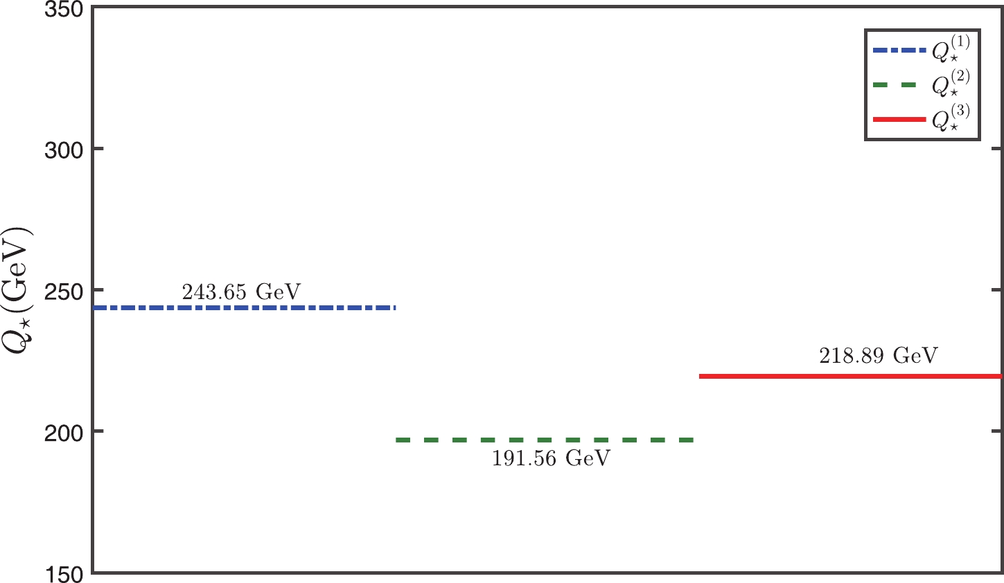
Figure 3. (color online) The determined effective scale
$ Q_\star $ .$ Q^{(1)}_\star $ is at the LL accuracy,$ Q^{(2)}_\star $ at the NLL accuracy and$ Q^{(3)}_\star $ at the$ {\rm N^{2}LL} $ accuracy.It is helpful to be able to estimate the “unknown” higher-order pQCD corrections. The conventional error estimate obtained by varying the scale over a certain range is not reliable, since it only partly estimates the non-conformal contribution but not the conformal one. The Pad
$ \acute{\rm{e}} $ approximation approach (PAA) provides a practical way of promoting a finite series of an analytic function [45–47], which was recently suggested to give a reliable prediction of uncalculated high-order terms by using the PMC conformal series [48].As an attempt, following the approach described in detail in Ref. [48], we give a PAA+PMC prediction for
$ R_{n}(M_{\rm H}) $ by using the preferable$ [0/(n-1)] $ -type Padé series. The results are presented in Fig. 4, where “PAA” is the predicted$ R_{n}(M_{\rm H}) $ by using the known$ R_{n-1}(M_{\rm H}) $ series, and “EC” is the prediction by directly using the known PMC$ R_{n}(M_{\rm H}) $ series. Figure 4 shows that the difference between “EC” and the predicted$ R_{n}(M_{\rm H}) $ tends to decrease as more higher-order loops are included. The difference between$ R_{3,4}(M_{\rm H})|_{\rm PAA} $ and$ R_{3,4}(M_{\rm H})|_{\rm EC} $ is already less than 1%, thus the “exact” value of$ R(M_{\rm H})|_{\rm EC} $ could be directly taken as$ R_{5}(M_{\rm H})|_{\rm PAA} $ , i.e.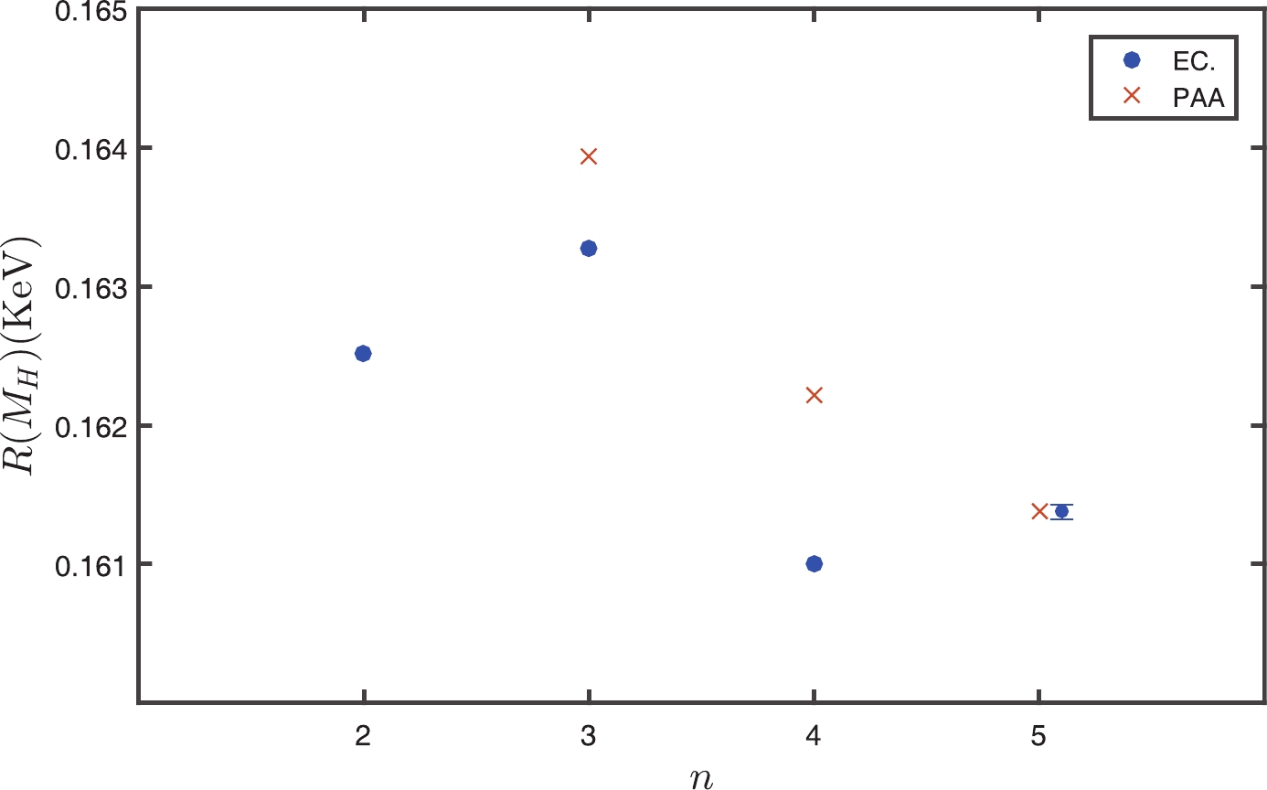
Figure 4. (color online) Comparison of the exact (“EC”) and the predicted [
$ 0/(n-1) $ ]-type “PAA” pQCD approximant$ R_{n}(M_{\rm H}) $ with the PMC scale-setting, showing how the PAA prediction changes when more loop terms are included.$ R_5(M_{\rm H})|_{\rm PAA} \cong 1.614\times10^{-1}\; {\rm KeV}. $

(24) The total decay width is then
$ \Gamma_5(H\to\gamma\gamma)|_{\rm PMC} = \left[9.626\pm5.354\times10^{-5}\right]\; {\rm KeV}, $

(25) where the error is the PAA+PMC prediction of uncalculated high-order pQCD contributions, which is negligible.
The total decay width
$ \Gamma(H\to\gamma\gamma) $ versus the Higgs mass$ M_{\rm H} $ is presented in Fig. 5. If we take the Higgs mass given by the ATLAS and CMS collaborations [49, 50], i.e.$ M_{\rm H} = 125.09\pm0.21\pm0.11 $ GeV, we obtain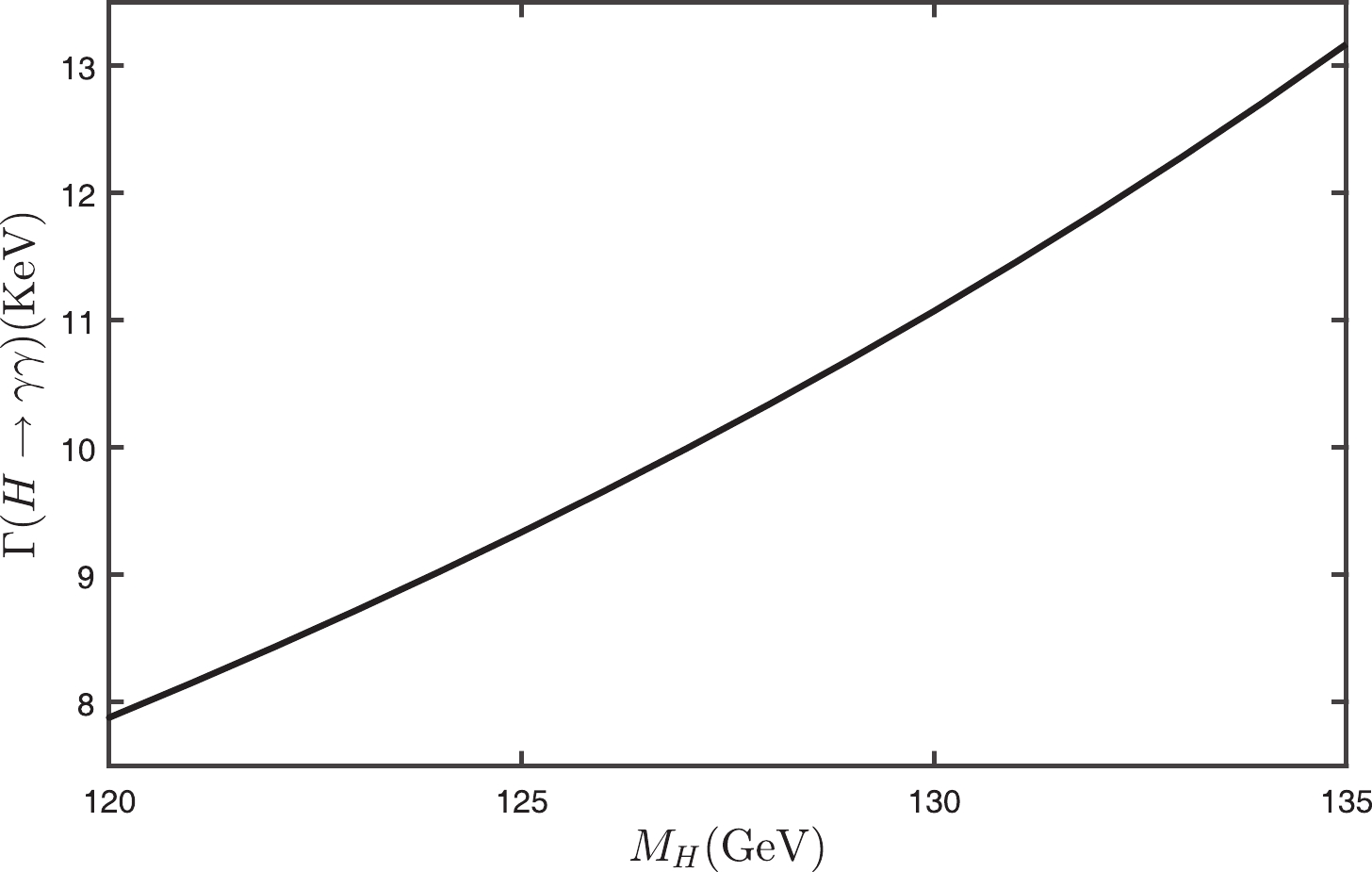
Figure 5. The PMC prediction of the decay width
$ \Gamma(H\to\gamma\gamma) $ versus the Higgs mass$ M_{\rm H} $ .$ \Gamma(H\to \gamma\gamma)|_{\rm LHC} = 9.364^{+0.076}_{-0.075} \; {\rm KeV}, $

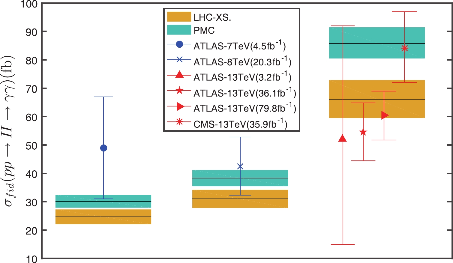
(26) As an application, we predict the “fiducial cross-section” of the process
$ pp\to H\to\gamma\gamma $ , which was predicted by the LHC-XS group with the conventional scale-setting [51] and was measured by the ATLAS and CMS collaborations with increasing integrated luminosity [52–54]. A PMC prediction was previously given in Ref. [55] by using$ \Gamma(H\to\gamma\gamma) $ up to N2LO. Taking the same parameters as in Refs. [51, 55, 56], e.g.$ M_{\rm H} = 125 $ GeV and$ M_t $ = 173.3 GeV, and by using the present$ \Gamma(H\to\gamma\gamma) $ up to N4LO, we obtain$ \sigma_{\rm fid}(pp\to H\to \gamma\gamma) = 30.1^{+2.3}_{-2.2} $ fb,$ 38.3^{+2.9}_{-2.8} $ fb, and$ 85.8^{+5.7}_{-5.3} $ fb for the proton-proton center-of-mass collision energy$ \sqrt{S} = 7 $ ,$ 8 $ and$ 13 $ TeV, respectively. Here, the errors are dominated by the error of the Higgs inclusive cross-section. A comparison with the recent experimental data is shown in Fig. 6. A better agreement with the data at$ \sqrt{S} = 7 $ and$ 8 $ TeV can be achieved by applying PMC. The ATLAS and CMS measurements at$ \sqrt{S} = 13 $ TeV still have large errors and are in disagreement, and the PMC prediction is closer to the CMS result. -
In summary, PMC uses the basic RGE to set the correct
$ \alpha_s $ running behavior. The resultant conformal series is independent of the initial choice of renormalization scale and renormalization scheme, and thus eliminates conventional scheme-and-scale ambiguities.Using the pQCD corrections up to the N4LO level, we can fix the effective PMC scale up to the N2LL level, and an accurate scheme-and-scale independent prediction for the decay width
$ \Gamma(H\to\gamma\gamma) $ can be achieved. Due to the elimination of divergent renormalon terms, the pQCD convergence can be naturally improved by applying PMC. This improvement of pQCD convergence has been found in most PMC applications. However, as shown in the case of the$ \gamma\gamma^*\to\eta_c $ form factor [57], where the magnitude of the NNLO term is still larger than the NLO term even after applying PMC, there may remain large logarithmic terms in the resultant PMC conformal series, diluting the pQCD convergence. In these special cases, the conventional resummation approach [58] may help to further improve the pQCD convergence. A detailed discussion on this point is in progress.
Properties of the decay ${{H\to\gamma\gamma}} $ using the approximate ${{\alpha_s^4}}$ corrections and the principle of maximum conformality
- Received Date: 2019-04-03
- Accepted Date: 2019-06-05
- Available Online: 2019-09-01
Abstract: The decay channel


 DownLoad: