Extinction coefficients of surface atmospheric aerosol above LHAASO

The Large High Altitude Air Shower Observatory(LHAASO), one of the Major National Science and Technology Infrastructures, is located at Haizi Mountain, Daocheng County, Sichuan Province. It is composed of the Square Kilometer Array (KM2A), Water Cherenkov Detector Array (WCDA), and Wide Field of view Cherenkov Telescope Array (WFCTA), and expected to be the highest sensitivity instrument in terms of gamma ray detection, ultra-high gamma surveys, and the primary cosmic ray spectra and anisotropy [1, 2]. WFCTA, consisting of 18 telescopes, has been designed to measure primary cosmic rays with the energy of 10¹³–10¹⁷ eV and transfer the energy scale from direct measurement to the extreme high-energy measurement, with different a lay-out in different observation modes and energy ranges [3, 4].

To meet the requirements of the calibration of WFCTA to effectively select good shower events and correct the raw data, as well as to improve the quality of the data and decrease systematic errors, it is of primary importance to investigate the variation of extinction coefficients from the surface atmospheric aerosol over LHAASO.

LHAASO (29°21′31″N, 100°08′15″E) is located in the east-south of Tibetan Plateau, and the western Sichuan Province. This region is mainly covered by the alpine grassland in summer, and by snow during cold winters. In the Tibetan Plateau, the atmospheric aerosols are usually taken as a whole and the geographical range is $ 30^\circ - 36^\circ$ in latitude, and $80^\circ - 100^\circ $ in longitude. The chemical composition and optical properties, like extinction coefficients together with aerosols optical depth, have been investigated by many atmospheric researchers [5-7]. The daily average of online PM2.5 at the southeast Tibetan Plateau, where LHAASO belongs, is 11.7 ± 4.7 µ gm⁻³, however the ratio of PM2.5 to the total suspended particles was higher than that at Ngri, Qomolangma and Nam Co, which probably originates from the Sichuan Basin with dense PM2.5 [8]. However, to date no studies performed on the extinction coefficients over LHAASO have been reported. In this study, we evaluate the extinction coefficients of surface atmospheric aerosol based on the Longtin model [9] and Mie scattering theory, which will be compared with results from the experimental data by CALIPSO/CALIOP. The results are expected to provide the theoretical arguments and references for our laser lidar calibration of LHAASO.

The classification method for atmospheric aerosols has still not been agreed upon by scientists. According to the content, atmospheric aerosols can be classified as burning aerosol, creature aerosol, and mineral dust aerosol [10]. Mineral dust aerosol is one of the main types of aerosols in the troposphere. Mineral dust particles are mainly emitted from arid and semiarid regions (e.g., Saharan and Gobi Deserts). Different types of aerosols are often mixed in the atmosphere (internal or external mixing) [11-13], especially in the East Asian region. Mineral dust is often mixed with man-made polluted aerosols on its transport path [14–15]. At the LHAASO site, sandy soil with sparse grass and small rocks cover the land surface, and a river of 1–3 m width flows from the southwest to the northeast. Because of the harsh nature of its environment, LHAASO is relatively isolated from industrial zones and cities, with a very limited local population. Mineral dust was identified as one of the main aerosol components in the central Tibetan Plateau [16]. The analysis of dust plumes from the surrounding deserts has indicated some potential source areas of atmospheric particles [17]. The particles of atmospheric aerosol above LHAASO probably comprise mineral dust. Usually, the extinction coefficient of atmospheric aerosol over the Tibetan Plateau is relatively smaller than that in the Sichuan Basin, which depicts the highly aerosol-polluted region in China. The chemical and physical properties of atmospheric aerosols over LHAASO have not been reported to date. In this study, mineral dust particles in the atmospheric aerosol are assumed to be spheres, and the extinction coefficients are evaluated based on the Mie scattering theory [18] and Longtin model [9].

The Longtin model was developed by David R. Longtin et al., and it is actually a wind-dependent desert aerosol model, firstly applied in the Air Force Geophysics Laboratory. In this model, mineral dust particles are separated into three major components depending on their composition, using different log-normal size distributions and sets of indices of refraction for each component. The components include carbonaceous particles, water soluble particles, and sand. The sand component consists of two kinds of particles, pure quartz and quartz contaminated with a small amount of hematite (iron oxide, Fe₂O₃). Local wind conditions provide the mechanism to inject and transport aerosols, while wind also provides a mechanism for the generation of additional aerosols by a sandblasting process. The change of size distribution and mass concentrations of the aerosols that are injected into the air is a result of wind erosion. In this model, the volume (mass) of the water soluble and carbonaceous particles remain the same as that for background condition, in which the volume fractions for carbonaceous particles, water soluble particles, and sand were calculated to be 0.299, 0.001, 0.70, respectively, using information on particle concentration and the volume of the single particle. The extra mass loading due to the wind arises from sand. The mass loading equation is the basis for the wind speed dependence, which is expressed as follows.

where c is the mass concentration in $ ug $ m⁻³ of air, u is the wind speed in m·s⁻¹ at a height of 10 m. Thus, the different size distribution and concentration for each component of the aerosol will be evaluated in the Mie scattering calculations based on the equation and local wind condition. More detailed parameters on each component are provided in Table 1 [9].

The Mie scattering calculation for the extinction coefficient, scattering coefficient, and absorption coefficient is performed separately for each component and then weighted according to their volume fraction of the total aerosol. The total coefficient is the sum of different components, as follows:

where i refers to the particle type.

Mie scattering occurs when the size of the aerosol particles is close to the wavelength of the incident light. To improve the calculation efficiency with the Mie scattering theory, D$ _n $ is defined as follows [19]:

Then, we have

where m is the complex refractive index of spherical particles relative to the ambient medium, $ x = k\alpha $ is the size parameter, $ \alpha $ the radius of the sphere and k = 2$ \pi/\lambda $, is the wave number and $ \lambda $ the wavelength in the ambient medium. $ \psi _n (x) $ is an equation related to semi-odd Bessel functions of the first kind, and $ \xi _n (x) $ is an equation related to semi-odd Hankel functions of the first kind.

Generally, the extinction efficiency factor $ Q_{\rm ext} $, scattering efficiency factor $ Q_{\rm sca} $, and absorption efficiency factor $ Q_{\rm abs} $, are referred to as the attenuation efficiency factor all together. $ Q_{\rm ext} $ denotes the ratio of extinction cross-sectional area to the maximum geometric area, and $ Q_{\rm abs} $, ratio of absorbtion cross-sectional area, $ Q_{\rm sca} $ has the similar definition.

When the imaginary part of the m and Im(m) are lower than $ 13.78({\rm Re}(m))^2-10.8{\rm Re}(m)+3.9 $ [20], the upward iteration method is more efficient than the downward iteration method, and the calculation error is guaranteed to be less than $ 10^{-10} $. The recurrence formula can be used to obtain $ D_n(mx) $

where $ D_0(mx) = {\rm cot}(mx) $. The iteration stops when $ n $ reaches $ n_{\rm max} $.

When $ {\rm Im}(m)> 13.78({\rm Re}(m))^2-10.8{\rm Re}(m)+3.9 $, downward iteration is selected, and its formula is

where $ \lim\limits_{n \to \infty}{D_n} = 0 $, $ D_n $ is calculated from $ n = n_{\max} $ to $ n = 1 $. $ n_{\rm start} $ equals to $ {\rm INT}(\max\{n_{\max},|mx|\}+16) $ and $ D_n|_{n = n_{\rm start}} = 0 $.

The extinction effect of atmospheric aerosol is the superposition of all effects from the aerosol particles in the air. The extinction coefficient $ k_{\rm ext} $, scattering coefficient $ k_{\rm sca} $, and absorption coefficient $ k_{\rm abs} $ describe the total optical attenuation. For atmospheric systems with uneven size distribution of the particles, the formula for the extinction coefficient is

where $ [r_{\min},r_{\max}] $ is the range of particle size, and $ N(r) $ is the distribution of particle concentration, which usually refers to the sum of several logarithmic normal distributions.

where $ N_i $ is particle number density, $ R_i $ is mean particle radius, and $ \lg \sigma _i $ is logarithmic standard variance.

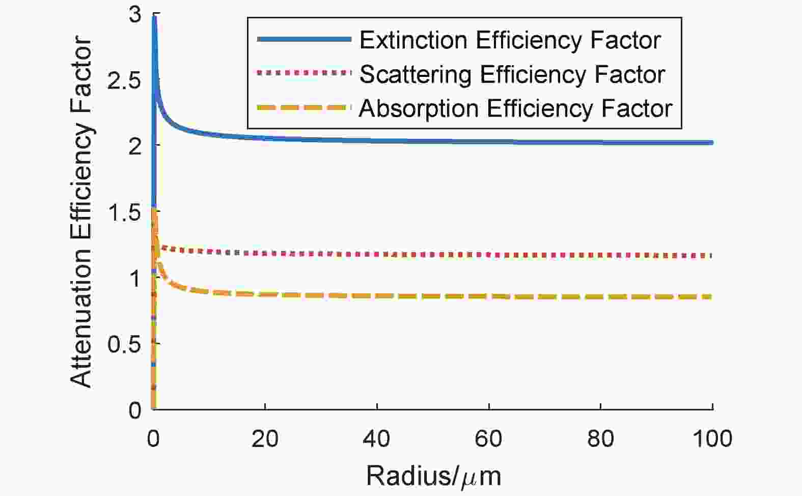
The detector on the CALIPSO emits the laser at a wavelength of 532 nm. Under this condition, the complex refractive indices $ m $ (assume the imaginary part is greater than 0) are as follows: $ 1.75+0.45i $ (carbonaceous particle), $ 1.53+10^{-7}i $ (water soluble particle), 1.548+ $ 10^{-8}i $ (sand containing pure quartz only), 1.607+3.98× $ 10^{-3}i $ (sand containing 5% hematite), and 1.666+8.09× $ 10^{-3}i $ (sand containing 10% hematite). During the calculations, we assume that sand particles comprise 50% sand of pure quartz only and 50% sand containing 10% hematite.

The results on the attenuation efficiency factors of the four types of particles are shown in Fig. 1 to Fig. 4, and each extinction efficiency factor exhibits drastic vibration when particle size is small. As the radius of particle is greater than 20 µm, $ Q_{\rm ext} $ is around two, while the absorption efficiency factors of water soluble particle and sand of pure quartz are close to zero. However, this is different for carbonaceous particles and sand containing 10% hematite. $ Q_{\rm abs} $ is, as the size of particle increases, stable around the value of one. Thus, a conclusion can be drawn that the real and imaginary parts of the complex refractive index are related to the scattering and absorption of light, respectively. When the imaginary part of $ m $ is relatively larger, the absorption efficiency factor is bigger.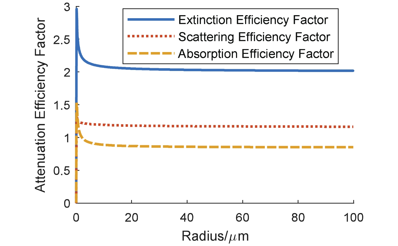

Figure 1.  (color online) Carbonaceous particle attenuation efficiency dependence on radius.

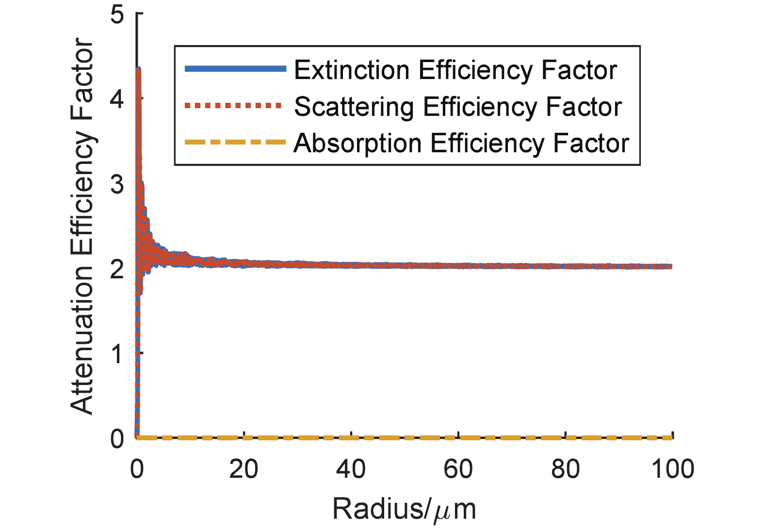
Figure 2.  (color online) Water soluble particle attenuation efficiency dependence on radius.

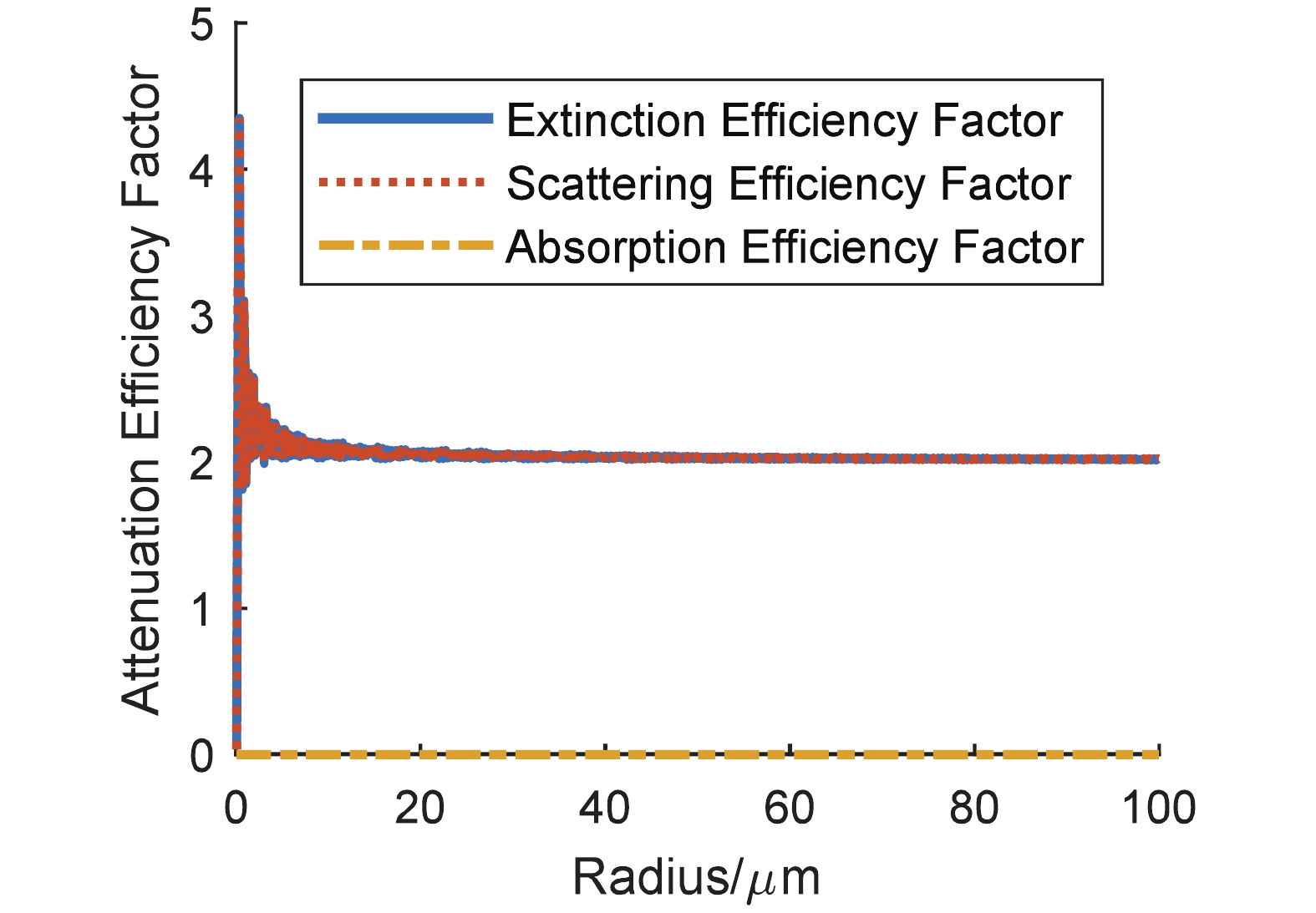
Figure 3.  (color online) Sand containing pure quartz only particle attenuation efficiency dependence on radius.

Figure 4.  (color online) Sand containing 10% hematite particle attenuation efficiency dependence on radius.

Using Equations (10)–(12) and related parameters, the extinction coefficients, dependent on wind speed and the wavelength of the income light, are presented in Fig. 5. As the wavelength increases, the extinction coefficient of particles decreases. When the wind speed rises, the size and concentration of sand in aerosol particles increase, so the extinction coefficient becomes bigger, too. The higher the wind speed is, the faster the extinction coefficient rises.

Figure 5.  (color online) Extinction coefficient of particles at different wavelengths and wind speeds.

During the period from July 16, 2015 to April 24, 2016, at the site of LHAASO station, a total of 6816 hours included wind occurrence, and this period can be used to calculate the local aerosol extinction coefficient. As the satellite observation data discussed below is collected mainly at around 7 p.m., the time interval of 7 p.m. to 8 p.m. is selected for theoretical calculation. In Fig. 6, the blue curve shows that the extinction coefficient varies with time, whereas the red curve represents the temporal variation extinction coefficient in the case of gust wind speed. The average wind speed is taken as the mean wind speed within one hour, and the gust wind speed is taken as the maximum value of the wind speed within one hour. Under average wind speed conditions, the extinction coefficient changes from 0.0415 km⁻¹ to 0.051 km⁻¹, whereas in the gust wind speed, which is generally high, the extinction coefficient is also high, ranging from 0.0414 km⁻¹ to 0.1041 km⁻¹.

Figure 6.  (color online) Theoretical value of night extinction coefficient at the site of LHAASO from July 16, 2015 to April 24, 2016.

The CALIPSO (Cloud-Aerosol Lidar and Infrared Pathfinder Satellite Observation), which was launched by NASA in April 2006, is located at 705 km above the earth at sun-synchronous orbit. The orbital inclination is 98.2 degrees. It obtains the three-dimensional distribution of global regional clouds and aerosols at an interval of 16 days. CALIOP (Cloud-Aerosol Lidar with Orthogonal Polarization) is the most important equipment carried by CALIPSO and provides high-resolution vertical profiles of aerosols and clouds. It has three receiver channels, one measuring the 1064 nm backscatter intensity and two channels measuring orthogonally polarized components of the 532 nm [21].

The data is selected from 99.6 degrees to 100.6 degrees east longitude and 29.0 degrees to 30.0 degrees north latitude, where the entire area of LHAASO is located. To ensure good quality of data, the cloud-aerosol distinguishing index is required to be within the range of –100 to –50 to better differentiate clouds and aerosols. Meanwhile, the uncertainty of the extinction coefficient should be less than 10, and the aerosol particle type should be determined. The coefficient ${\rm Ectinction\_ QC\_ 532} $ is set 0 or 1. Because of the distraction of sunlight during the daytime, a higher threshold is set during daytime. All data in this analysis are observed at night, and for the WFCTA of LHAASO, data is calibrated during the clear nights.

The height resolution of CALIPSO is 30 m, and the mean latitude of LHAASO is 4410 m a.s.l.. The average of the extinction coefficients at 4409 m a.s.l. and 4349 m a.s.l. is taken as the actual extinction coefficient of surface atmospheric aerosols above the LHAASO site. Fig. 7 illustrates the extinction coefficient as a function of time, from Oct. 2015 to April 2016 at the surface of the LHAASO site (data from CALIPSO Version 4.1 Level 2). The extinction coefficient at the 532 nm wavelength of the laser between October 2015 to March 2016 is about 0.02 km⁻¹, while it increased to 0.07 km⁻¹ in April 2016. However, the average extinction coefficient at 532-nm wavelength of the laser in the Tibetan Plateau is ~0.0083 km⁻¹ in spring and summer, ~0.0015 km⁻¹ in winter, and ~0.0008 km⁻¹ in fall [6]. Hence, the extinction coefficient at surface LHAASO site is higher than the average in the Tibetan Plateau. Compared with the theoretical value of $ k_{\rm ext} $, the experimental values lie at about half of them. MODIS and CALIOP are both sensors that are carried by A-Train series satellites. The difference of their transit time is only 90 seconds, such that the change of the extinction coefficient of aerosols at the same place observed by the two detectors can be ignored. The observation of aerosol optical depth in the data shows that the signal-to-noise ratio (SNR) of laser transmitted by CALIOP sensor on the ground is reduced [5], which probably leads to the smaller value of the extinction coefficient.

Figure 7.  (color online) Extinction coefficient during the period from Oct. 2015 to April 2016 at LHAASO.

LHAASO is one of the major national science and technology infrastructures that is currently under construction now. This study focuses on the extinction of surface atmospheric aerosol above LHAASO and estimates the extinction coefficient quantitatively using the Longtin model. The extinction coefficient is related to the wind speed. Supposing the wavelength of incoming light is 532 nm, the extinction coefficient of atmospheric aerosols varies from 0.0420 km⁻¹ to 0.229 km⁻¹ as the wind speed increases from 0 ms⁻¹ to 20 ms⁻¹. The extinction coefficient from CALIOP/ CALIPSO is compared with the theoretical calculation based on the Mie scattering theory and Longtin Model.

The relative humidity (RH) in the atmosphere has significant daily and seasonal variations. The hygroscopic growth of optical properties of atmospherics aerosols largely depend on the RH [22–24]. As RH increases, the extinction coefficient grows and favors a more rapid growth when aerosol contains a high content of inorganic water-soluble salts [25–27]. In the Longtin model, the atmospheric aerosols have a water-soluble component, but the influence of relative humidity on the extinction coefficient is not considered.

According to the observations from CALIOP, the studied region's extinction coefficient is higher than the average level of Tibetan Plateau, however lower than the theoretical estimate. This may be related to the particle content in the model. In the Longtin model, the background components represent carbonaceous particles, water soluble particles, and sand. The volume fractions of these three kinds of particles are 0.001, 0.299, and 0.70, respectively. Supposing the total volume proportion of the atmospheric aerosols to the air is the same as that in the background condition, and the wind speed is zero, the extinction coefficient from atmospheric aerosols is almost maintained at ~0.04 km⁻¹ when only the water soluble particles or sand changes are assumed unchanged, and volume fractions of the other two components change in a realistic range. However, the extinction coefficient changes significantly if we assume that the volume fraction of the carbonaceous component remains unchanged, whereas the volume fraction of water soluble particles and sand is altered. We designate the volume fraction of water soluble particles V₁, and the volume fraction of sand V₂. As shown in Fig. 8, the extinction coefficients depend on the ratio of $ V_1 $ to $ V_2 $(V₁/V₂), and are reducedto 0.015 km⁻¹ when $ V_1/V_2 $ is 0.11. This means that a lower quantity of water soluble particles and a higher quantity of sand particles within the aerosol particles mix leads to a smaller extinction coefficient. Moreover when the quantity of aerosols in the atmosphere in the Longtin model decreases, the extinction coefficient becomes smaller.

Figure 8.  (color online) Extinction coefficient dependence on the ratio V₁ to V₂(V₁/V₂). V₁ represents the volume fraction of water soluble particles, V₂ depicts the volume fraction of sand. The red point depicts the extinction coefficient calculated with the volume fraction in the background condition of the Longtin model.

The shape, size distribution, mass concentration, RH dependence, wind speed dependence, and other properties of aerosol particles above this site will be studied further in a future study to determine the variations in the extinction coefficient.

The authors would like to thank Dr. Xiaojun Ma and Professor Zhongwei Huang of Lanzhou University for their help in the data analysis of CALIPSO data.

CALIPSO data were obtained from the NASA Langley Research Center Atmospheric Sciences Data Center.