


 Abstract
 HTML
HTML Reference
 Related
 PDF
PDF


-
The nuclear landscape is categorized into different regions, where the valley of stability is situated almost at the center containing around 288 stable nuclei. By adding nucleons, we move away from the valley of stability and enter into the vast zone of short lived radioactive nuclei, which decay by
$ \alpha $ and$ \beta $ - particle emission or split into smaller parts through spontaneous fission. Moving away from the valley, a point comes where the binding energy is insufficient to hold the last nucleon, and hence it gets emitted. These extreme points create a boundary for the nuclear landscape, known as the proton drip line on the one side, represented by Protactinium (Z = 91), and the neutron drip line on the other side, given by Oxygen (Z = 8), both determined experimentally [1]. The phenomenon of nucleon emission from the nuclear ground state limits the possibility of creation of more exotic nuclei in the nuclear landscape. The study of exotic nuclei includes many predicted and observed novel facts such as the change of the magic number, shape discrimination between core and halo [2], giant halo [3, 4], and is an indispensable factor in the contemporary nuclear physics. Specifically, exotic nuclei above the drip lines show great challenges to both experimental and theoretical physicists.Proton emitters lie above the proton drip line with the proton decay energy
$ Q_{p}>0 $ for spontaneous proton emission. Proton emission does not only give information on the interaction of the nucleons near the drip line, but also provides spectroscopic information because the decay rate of unpaired decaying proton is sensitive to the Q value and orbital angular momentum ($ \ell $ ) , which in turn helps to determine the$ \ell $ value of the emitted proton. The$ \ell $ value is a prime quantity to explore the anomaly in the shell structure of the proton rich nuclei involved in the process. Proton radioactivity also provides invaluable information on the nuclear force beyond the drip line region.Experimentally, the first proton emitter was discovered as an isomeric state of
$ ^{53}{\rm Co}^{*} $ in 1970 [5, 6]. Since then, more than 30 proton emitters have been observed in the region around I to Bi, with the proton number from Z = 53 to 83 [7, 8]. Many theoretical studies have been carried out to understand the physics beyond the drip line [9-13]. In addition, the simple cluster model [14], the effective liquid drop model of heavy particle decay [15], and the unified fission model by Gupta et al. [16], where the pre-formed cluster model is modified with the effects of Coulomb repulsion, nuclear attraction by proximity potential and rotational energy, were studied. Similarly, the folding model analysis of proton radioactivity by single folding of the densities of the daughter nucleus with the effective M3Y nucleon-nucleon interaction [17] and with the M3Y + EX and R3Y + EX interactions [18] , provide reasonable results for the observed proton-radioactivity life time. The relativistic continuum Hartree-Bogoliubov theory (RCHB) [19, 20] , with the relativistic energy density PC-PK1 functional [21] , was used to examine the phenomenon of proton emission from both the ground and isomeric states, and to calculate the half-life of proton emitters in the region of the proton drip line. All these studies produce results that agree well with the experimental data.The finite and infinite nuclear matter have been successfully studied using the effective relativistic mean-field (E-RMF) approach [22]. In this approach, the experimental values of finite nuclear properties, such as the binding energy, root mean square radius etc., are very well reproduced [23]. The E-RMF model starts from the Lagrangian of the system which includes the self- and cross- couplings of isoscalar-scalar
$ \sigma $ , isoscalar-vector$ \omega $ , isovector-scalar$ \delta $ , and isovector-vector$ \rho $ mesons. Each meson coupling has its own importance in describing the nuclear properties [24].The original formula for E-RMF of Frunstahl et al. [25] analyzed the nuclear properties without the inclusion of isovector-scalar
$ \delta $ meson and the cross coupling of$ \rho $ and$ \omega $ mesons. The effects of$ \delta $ meson and the cross coupling of$ \rho $ and$ \omega $ mesons were included by J. K. Bunta et al. [26] and C. J. Horowitz et al. [27]. Although the inclusion of$ \rho $ meson takes care of the bulk properties of the nucleus arising from the isovector part, the contribution of$ \delta $ meson becomes very important for studying the drip line or highly asymmetric nuclei, which can be found in refs. [28-40]. In this context, we have used the E-RMF formalism with the inclusion of$ \delta $ meson and the cross coupling of$ \omega $ and$ \rho $ mesons to study the bulk properties of proton rich nuclei.The paper is divided into following sections. Section 2 is devoted to the brief description of E-RMF and the formalism used in the present study. The results of our calculations and discussions are presented in Section 3, and the conclusion drawn from the study is given in Section 4.
-
To study the highly asymmetric system, we assume the E-RMF model, where the energy density functional
$ {\cal E}({r}) $ includes the contributions from the self- and cross- couplings of$ \sigma $ ,$ \omega $ ,$ \rho $ and$ \delta $ mesons and photon A. In this section we briefly summarize the E-RMF energy density functional which reads as [25, 40, 41, 42],$ \begin{split} {\cal E}({r}) = & \sum_\alpha \varphi_\alpha^\dagger({r}) \Bigg\{ -i {{\alpha}} \!\cdot\! {\bf{\nabla}} + \beta \left[M-\Phi (r)-\tau_3 D(r)\right] \\ & + W({r}) + \frac{1}{2}\tau_3 \rho^{\mu}({r}) + \frac{1+\tau_3}{2} A ({r}) \\ & - \frac{i \beta{{\alpha}}}{2M}\!\cdot\! \left (f_\omega {\bf{\nabla}} W({r}) + \frac{1}{2}f_\rho\tau_3 {\bf{\nabla}} \rho^{\mu}({r}) \right)\Bigg\} \varphi_\alpha (r) \\ & + \left ( \frac{1}{2} + \frac{\kappa_3}{3!}\frac{\Phi({r})}{M} + \frac{\kappa_4}{4!}\frac{\Phi^2({r})}{M^2}\right ) \frac{m_\sigma^2}{g_\sigma^2} \Phi^2({r}) \\ & - \frac{\zeta_0}{4!} \frac{1}{ g_\omega^2 } W^4 ({r}) + \frac{1}{2g_\sigma^2}\left( 1 + \alpha_1\frac{\Phi({r})}{M}\right) \left( {\bf{\nabla}}\Phi({r})\right)^2 \\ & - \frac{1}{2g_\omega^2}\left( 1 +\alpha_2\frac{\Phi({r})}{M}\right) \left( {\bf{\nabla}} W({r}) \right)^2 \\ & - \frac{1}{2}\left(1 + \eta_1 \frac{\Phi({r})}{M} + \frac{\eta_2}{2} \frac{\Phi^2 ({r})}{M^2} \right) \frac{m_\omega^2}{g_\omega^2} W^2 ({r}) \\ & - \frac{1}{2e^2} \left( {\bf{\nabla}} A({r})\right)^2 - \frac{1}{2g_\rho^2} \left( {\bf{\nabla}} \rho^{\mu}({r})\right)^2 \\ & - \frac{1}{2} \left( 1 + \eta_\rho \frac{\Phi({r})}{M} \right) \frac{m_\rho^2}{g_\rho^2} {\rho^{\mu}}^2({r}) -\Lambda_{\omega}\left({\rho^{\mu}}^{2}(r)\times W^{2}(r)\right) \\ & +\frac{1}{2 g_{\delta}^{2}}\left( {\bf{\nabla}} D({r})\right)^2 +\frac{1}{2}\frac{ { m_{\delta}}^2}{g_{\delta}^{2}}\left(D^{2}(r)\right)\;, \end{split} $

(1) where
$ m_{\sigma} $ ,$ m_{\omega} $ ,$ m_{\rho} $ and$ m_{\delta} $ ,$ g_{\sigma} $ ,$ g_{\omega} $ ,$ g_{\rho} $ and$ g_{\delta} $ and$ \Phi $ ,$ W $ ,$ \rho^{\mu} $ and$ D $ are the masses, coupling constants and fields for the$ \sigma $ ,$ \omega $ ,$ \rho $ and$ \delta $ mesons, respectively.$ e^{2}/4\pi $ and$ A_{\mu} $ are the coupling constant and the field of a photon, respectively. The fields for the mesons are constructed from the Klein-Gordon equation, and the nucleon dynamics are taken care by the Dirac equation. The set of E-RMF equations is solved numerically by a self consistent iteration method using the NL3 [43], FSUGarnet [44], G3 [24] and IOPB-I [45] parameter sets to obtain the ground state properties and the spherical matter densities, which are used for further formulation to get the effective nuclear interaction potential.In the open-shell nuclei, the pairing correlation plays an important role. For nuclei near the stability line, simple BCS approximation with a constant gap [46, 47] is an appropriate formalism for the pairing effect. However, it fails to describe the pairing effect in the drip line nuclei. This is because the constant gap between the levels is lost as we move away from the stability line. For such nuclei, the increase in the number of neutrons or protons drive the Fermi level to zero, and the availability of levels above the Fermi surface is reduced. In such a situation, the continuum states are significantly populated and the particle-hole and pairing excitation reach continuum. To overcome this problem, the BCS formalism is modified by taking into account the continuum effects by means of the quasibound states [48, 49] (states that are bound by their own centrifugal-plus-Coulomb barrier). In this approach, we restrict the region of influence of the pairing potential to the vicinity of the Fermi level. The relativistic Lagrangian contains only the term
$ \varphi^\dagger\varphi $ , and no terms of the type$ \varphi^\dagger\varphi^\dagger $ or$ \varphi\varphi $ (responsible for the pairing effect) are found. In the mean-field approach, the mean of the above terms vanishes. Hence, it becomes necessary for the present calculations to include the paring correlation externally using the quasi-bound BCS approximation.The decay process of proton emission can be viewed as a simple quantum tunneling effect through a potential barrier created by the emitted proton and daughter nucleus interaction. The daughter nucleus density is taken from the E-RMF calculations, and the proton density is extracted from the experimental scattering data [50]. We construct the nuclear potential for the daughter-emitter system by folding the two densities with the help of the double folding model [51]. The Coulomb and centrifugal potential is then added to get the effective interaction potential. As most proton emissions are likely to take place from the orbitals with
$ \it{l} \neq 0 $ , it become important to add the centrifugal part. However, the centrifugal part is less ambiguous for alpha or other exotic decays. The total interaction potential is then the sum of the nuclear potential, Coulomb potential and centrifugal potential, represented as,$ V(R) = V_{N}(R) + V_{C}(R) + \frac {{\hbar}^{2}}{2 \mu R} l(l+1) \;, $

(2) where R is the separation between the center-of-mass of the daughter nucleus and emitted proton,
$ \ell $ is the orbital angular momentum of the emitted proton, and$ \mu $ is the reduced mass of the proton-daughter system. The nuclear potential$ V_{N}(R) $ is obtained by double folding the daughter nucleus and emitted proton densities with the realistic M3Y effective interaction, given by the equation,$ V_{N}(R) = {\int {\rm d}r_{1}{\int {\rm d}r_{2} \rho_{1}(r_{1})\rho_{2}(r_{2}) V_{NN}(r_{12} = R+r_{2}-r_{1})}}, $

(3) where
$ r_{1} $ and$ r_{2} $ are the respective position co-ordinates of the emitted proton and daughter nucleus with respect to their centers.$ \rho_{1}(r_{1}) $ and$ \rho_{2}(r_{2}) $ are the proton and daughter densities, respectively.$ V_{NN}(r_{12}) $ is the effective nucleon-nucleon M3Y interaction.The Coulomb potential is given by,
$ \begin{split} V_{C}(R) &= Z_{p}Z_{d}e^2/R\;\quad\quad\;\;\;\;\quad\quad\quad\quad {\rm for}\;\; R > R_{c} \\& = (Z_{p}Z_{d}e^2/2R_{c})\left[3-\left(\frac{R}{R_{c}}\right)^2\right] \;\;\;{\rm for} \;\;R \leqslant R_{c}\;, \end{split} $

(4) where
$ Z_{p} $ and$ Z_{d} $ are the atomic numbers of the proton and daughter nucleus, respectively.$ R_{c} = 1.2\left(A_{p}^{1/3}+A_{d}^{1/3}\right) $ is the touching radial separation between the proton and daughter nucleus.For the calculation of the proton emission half-life (
$ T_{1/2} $ ) we adopt the Wentzel-Karmers-Brillouin (WKB) method. In this method, the penetration probability is given by,$ P = \exp[-2{\int \frac{\sqrt{2m}}{\hbar} [V(R)-Q_{p}]^{1/2} {\rm d}R]} \;. $

(5) $ Q_{p} $ is the Q value for proton emission, and the limits of integration are the turning points where$ V(R = r_{1}) = $ $ V(R = r_{2}) = Q_{p} $ . This means that the tunneling of the proton begins at$ r_{1} $ and terminates at$ r_{2} $ . In our calculations, we used the preformed cluster model (PCM) of Gupta and collaborators [52-54] , in which the decay constant is given as,$ \lambda = P_{0} \nu_{0} P \;, $

(6) where
$ \nu_{0} $ is the assault frequency with which the proton hits the barrier. Since the proton is already present inside the parent nucleus, the preformation probability$ P_{0} $ is taken to be 1. From Eq. (6), we get the proton emission half-life as,$ T_{1/2} = {\rm ln}2/\nu_{0}P \;. $

(7) -
In the Walecka model, the nuclear interaction is understood through the nucleon-meson interaction. Due to the absence of meson-meson coupling, the incompressibility of the nuclear matter was found to be higher than the experimental value of 210 ± 30 MeV [55] , as the value found from the Walecka model is ≈ 550 MeV. It was then attempted to include the self and cross coupling terms of mesons. Boguta and Bodmer for the first time inserted the self-coupling terms of
$ \sigma $ meson, which brings the nuclear incompressibility to the acceptable range of 211 MeV for infinite nuclear matter at saturation [56-58]. In addition, the inclusion of the non-linear self coupling of$ \sigma $ meson reproduces the repulsive part of the nucleon-nucleon (NN) potential at long range, and also improves the finite nuclear properties [59]. In spite of the successful contribution of$ \sigma $ meson in describing finite nuclear matter, the equation-of-state (EOS) was still not described satisfactorily. However, inclusion of the self interaction term of the vector meson$ \omega $ was found to describe the EOS remarkably well [60, 61]. After inclusion of the non-linear terms of the above two mesons, the saturation properties of nuclei are very well understood. Furthermore, in the studies of heavy nuclei for which$N \gg Z $ , the inclusion of additional meson interactions was found to be necessary. This problem was overcame by Todd-Rutel and Piekarewicz by introducing the cross coupling of$ \omega $ and$ \rho $ mesons, which take care of the neutron skin thickness and the radius of neutron stars [62]. Recently, a series of new parameter sets, such as FSUGarnet, G3, IOPB-I are reported [24, 44, 45]. In these sets, additional interactions of mesons, e.g.$ \delta $ meson, and higher order interactions of various cross-couplings, are included for various reasons. One remarkable property of these sets is the matching of the results in EOS at the low density region of empirical values. These sets also reproduce the neutron skin thickness much better than the older ones [45].In this context, we used four parameter sets, namely NL3 [43], FSUGarnet [44], G3 [24] and IOPB-I [45] to study the properties of proton emitters. Among them, NL3 is the oldest, successful and popularly used parameter set for describing many properties of finite nuclei in the whole mass range. It includes only the self coupling of
$ \sigma $ meson. The sets FSUGarnet and IOPB-I, on the other hand, include the additional self-coupling of$ \omega $ meson, and the cross coupling of$ \omega $ and$ \rho $ mesons. They are successful in reproducing the lower and upper limits of the neutron star masses, i.e. M = 2.06$ M_{\odot} $ and M = 2.15$ M_{\odot} $ , respectively. The remaining set G3, along with all the above interactions of different mesons, includes the contribution of$ \delta $ meson. This set is quite successful in estimating the mass and radius of neutron stars, and also describes the bulk properties of finite and infinite nuclear matter. -
In this work, we considered the proton emitters from I to Bi with Z = 53 to 83 and N = 56 to 102 in their ground state. Calculations were carried out assuming the proton emitters to be spherical in shape. We used the E-RMF formalism with the interactions NL3 [43], FSUGarnet [44], G3 [24] and IOPB-I [45] for the analysis of the ground state properties, such as the binding energy per nucleon (B/A) and the neutron skin thickness (
$ \Delta r_{n} $ ). The decay half-life of the proton emitters was calculated in the E-RMF environment using the WKB method for the same four interactions. The experimental values were taken for the Q value of the decay process [63]. Finally, the calculated results for the half-life of proton emitters were compared with the experimental values [64, 65] and other theoretical studies [16, 18, 21] -
Binding energy per nucleon (B/A) is the measure of cohesiveness of the individual nucleons. It varies with the atomic mass number A. B/A of proton emitters, assuming a spherical shape of nuclei from Z = 53 - 83 and N = 56 - 102 , are given in Table 1 , columns 2 to 5 for NL3, G3, FSUGarnet and IOPB-I interactions, respectively, and columns 6 and 7 for PC-PK1 [66, 67] and the experimental values [64]. From the tabulated values, we find that the calculated results are quite close to PC-PK1 and the experimental data. B/A of the considered elements lie in the region of stability of the B/A curve near the iron peak. Looking at the B/A values one may think that these elements are stable, but this is not the case as they undergo particle emission. Now, let us study the above scenario in more detail. In the N-Z plane, the ideal case for existence of a nucleus is that it lies on the N = Z line. However, beyond Z
$ \approx $ 10 , the number of neutrons increases more rapidly than the number of protons in order to compensate the Coulomb force between protons. Hence, the stability curve tilts towards the neutron axis, indicating the requirement of a larger number of neutrons for the existence of these elements. For example,$ {^{109}_{\phantom{1}53}}{\rm I} $ , considered in this work, has Z = 53 and N = 56, whereas the stable isotopes of iodine require around 75 neutrons to fully compensate the Coulomb force. In the present case, 56 neutrons are insufficient to hold the nucleons in the most stable state. Hence,$ ^{109}_{\phantom{1}53}{\rm I} $ lies slightly away from the$ \beta $ -stability line, i.e. in the proton drip line. In addition, the nuclear force acting between the neutron-proton, proton-proton and neutron-neutron is found to be repulsive in their singlet-singlet or triplet-triplet configurations. Hence, the outer protons, lying on the surface of the nucleus, suffer from both the Coulomb and nuclear repulsive forces. Moreover, due to the decrease in the strength of the binding energy in the outer orbitals, the outer protons are loosely bound. Hence, despite the large binding energy per nucleon, due to the above factors, the proportionality between the neutron and proton arrangement breaks down and the outer proton gets emitted.nucleus B/A $ \Delta r_{n} $ 

NL3 FSUGarnet G3 IOPB-I PC-PK1 [67] Expt. [64] NL3 FSUGarnet G3 IOPB-I PC-PK1 [67] $ ^{109}_{\phantom{1}53}{\rm I} $ 

8.190 8.173 8.161 8.177 8.16 8.220 −0.0362 −0.0532 −0.0471 −0.0467 −0.031 $ ^{112}_{\phantom{1}55}{\rm Cs}$ 

8.071 8.049 8.032 8.059 8.100 −0.0533 −0.0653 −0.0630 −0.0611 $ ^{113}_{\phantom{1}55}{\rm Cs}$ 

8.116 8.096 8.070 8.106 8.06 8.1481 −0.0417 −0.0568 −0.0515 −0.0511 −0.037 $ ^{117}_{\phantom{1}57}{\rm La}$ 

8.035 8.012 7.994 8.024 8.088 −0.0366 −0.0501 −0.0533 −0.0447 $ ^{131}_{\phantom{1}63}{\rm Eu}$ 

7.894 7.879 7.881 7.887 7.89 7.995 −0.0275 −0.0560 −0.0483 −0.0450 −0.03 $ ^{140}_{\phantom{1}67}{\rm Ho}$ 

7.832 7.821 7.823 7.824 7.906 −0.0254 −0.0537 −0.0485 −0.0426 $ ^{141}_{\phantom{1}67}{\rm Ho}$ 

7.871 7.861 7.863 7.862 7.87 7.943 −0.0133 −0.0442 −0.0396 −0.0316 −0.016 $ ^{144}_{\phantom{1}69}{\rm Tm}$ 

7.796 7.785 7.786 7.785 7.85 −0.0299 −0.0567 −0.0537 −0.0473 $ ^{145}_{\phantom{1}69}{\rm Tm}$ 

7.838 7.829 7.828 7.826 7.83 7.891 −0.0185 −0.0479 −0.0450 −0.0360 −0.02 $ ^{146}_{\phantom{1}69}{\rm Tm}$ 

7.879 7.872 7.868 7.866 7.87 7.913 −0.0075 −0.0396 −0.0367 −0.0261 −0.009 $ ^{147}_{\phantom{1}69}{\rm Tm}$ 

7.919 7.915 7.907 7.907 7.91 7.951 0.0028 −0.0325 −0.0288 −0.0176 0.002 $ ^{150}_{\phantom{1}71}{\rm Lu}$ 

7.822 7.856 7.842 7.845 7.84 7.867 −0.0025 −0.0447 −0.0417 −0.0314 −0.012 $ ^{151}_{\phantom{1}71}{\rm Lu}$ 

7.864 7.902 7.883 7.888 7.88 7.903 0.0061 −0.0376 −0.0341 −0.0230 −0.004 $ ^{155}_{\phantom{1}73}{\rm Ta}$ 

7.852 7.882 7.862 7.867 7.86 7.856 −0.0008 −0.0438 −0.0393 −0.0291 −0.008 $ ^{156}_{\phantom{1}73}{\rm Ta}$ 

7.895 7.892 7.873 7.877 7.87 7.871 0.0011 −0.0360 −0.0303 −0.0199 0.001 $ ^{157}_{\phantom{1}73}{\rm Ta}$ 

7.905 7.901 7.884 7.887 7.88 7.896 0.0106 −0.0289 −0.0216 −0.0113 0.011 $ ^{160}_{\phantom{1}75}{\rm Re}$ 

7.830 7.824 7.803 7.810 7.8 7.809 −0.0046 −0.0402 −0.0318 −0.0245 −0.004 $ ^{161}_{\phantom{1}75}{\rm Re}$ 

7.844 7.838 7.817 7.824 7.82 7.836 0.0038 −0.0342 −0.0239 −0.0170 0.007 $ ^{164}_{\phantom{1}77}{\rm Ir}$ 

7.777 7.768 7.742 7.755 7.73 7.748 −0.0103 −0.0442 −0.0335 −0.0292 −0.008 $ ^{165}_{\phantom{1}77}{\rm Ir}$ 

7.795 7.787 7.759 7.774 7.76 7.777 −0.0025 −0.0387 −0.0261 −0.0225 0.002 $ ^{166}_{\phantom{1}77}{\rm Ir}$ 

7.812 7.805 7.775 7.792 7.76 7.866 0.0049 −0.0335 −0.0190 −0.0161 0.008 $ ^{167}_{\phantom{1}77}{\rm Ir}$ 

7.830 7.824 7.791 7.810 7.79 7.812 0.0121 −0.0285 −0.0123 −0.0101 0.017 $ ^{170}_{\phantom{1}79}{\rm Au}$ 

7.772 7.763 7.726 7.752 7.71 7.729 0.0013 −0.0354 −0.0207 −0.0192 0.005 $ ^{171}_{\phantom{1}79}{\rm Au}$ 

7.792 7.784 7.744 7.773 7.74 7.754 0.0084 −0.0307 −0.0146 −0.0133 0.013 $ ^{176}_{\phantom{1}81}{\rm Tl}$ 

7.750 7.741 7.710 7.730 7.7 7.708 0.0233 −0.0189 −0.0046 −0.0001 0.019 $ ^{177}_{\phantom{1}81}{\rm Tl}$ 

7.762 7.755 7.725 7.742 7.72 7.732 0.0336 −0.0114 0.0028 0.0089 0.028 $ ^{185}_{\phantom{1}83}{\rm Bi}$ 

7.743 7.739 7.718 7.725 7.71 7.732 0.0706 0.0146 0.0280 0.0405 0.051 Table 1. The binding energy per nucleon (B/A) in MeV and the skin thickness (
$ \Delta r_{n} $ ) in fm are shown for proton emitters using the parameter sets NL3, FSUGarnet, G3 and IOPB-I. The experimental data for B/A [64] and the theoretical data [67] using PC-PK1 [66] are also shown for validation of our results. -
When the proton and neutron distributions are not symmetric inside the nucleus, the excess number of particles smear out of the core of the nucleus, which we call a skin. When the excess protons produce the skin, we call this a proton skin, and similarly, when the skin is due to excess neutrons, we call it a neutron skin. The neutron skin thickness is usually defined as
$ \Delta r_{n} = r_{n} - r_{p} $ , where$ r_{n} $ and$ r_{p} $ stand for radial distributions of neutrons and protons, respectively. Columns 8 to 11 in Table 1 give the neutron skin thicknesses of proton emitters in their ground state obtained from the spherical E-RMF formalism, while column 12 gives the PC-PK1 results for comparison. From the table we see that the$ \Delta r_{n} $ values from the theoretical calculations are quite comparable. We observe that almost all elements have negative values of$ \Delta r_{n} $ , which means that$ r_{p} $ is larger than$ r_{n} $ . But, if we look at the number of protons and neutrons, all elements have more neutrons than protons. We are also aware of the fact that for the physical existence of a heavy nucleus, the number of neutrons should be larger than the number of protons, in order to compensate the repulsive Coulomb force between protons. Although proton emitters have more neutrons than protons, their radial distribution$ r_{n} $ is less than$ r_{p} $ . This is due to the fact that all neutrons are involved in the compensation of the Coulomb force between protons, and, moreover, due to the strong neutron(n)-proton(p) interaction, they form a tightly bound np core of the nucleus. Still, the number of neutrons is insufficient to fully compensate the Coulomb force, as a result of which some protons are repelled outwards (towards the surface of the nucleus), forming a very thin proton skin, as observed from the tabulated values. Due to the small value of$ \Delta r_{p} $ , we cannot exactly say that it as a proton skin, rather we can say that these are protons which lie outside the core and on the surface of the nucleus. In this situation, these protons are very loosely bound and they become more prone to be emitted. From Table 1, we can see that for most elements,$ \Delta r_{n} $ is negative for all four parameter sets. However, around 12 cases with different (Z, N) combinations for NL3, only one combination (83, 102) for all parameter sets, and (81, 96) combination for all except the FSUGarnet set, and similarly for PC-PK1 for 8 such cases, have a value of$ \Delta r_{n} $ that is positive but around zero, which does not mean that it is a neutron skin. -
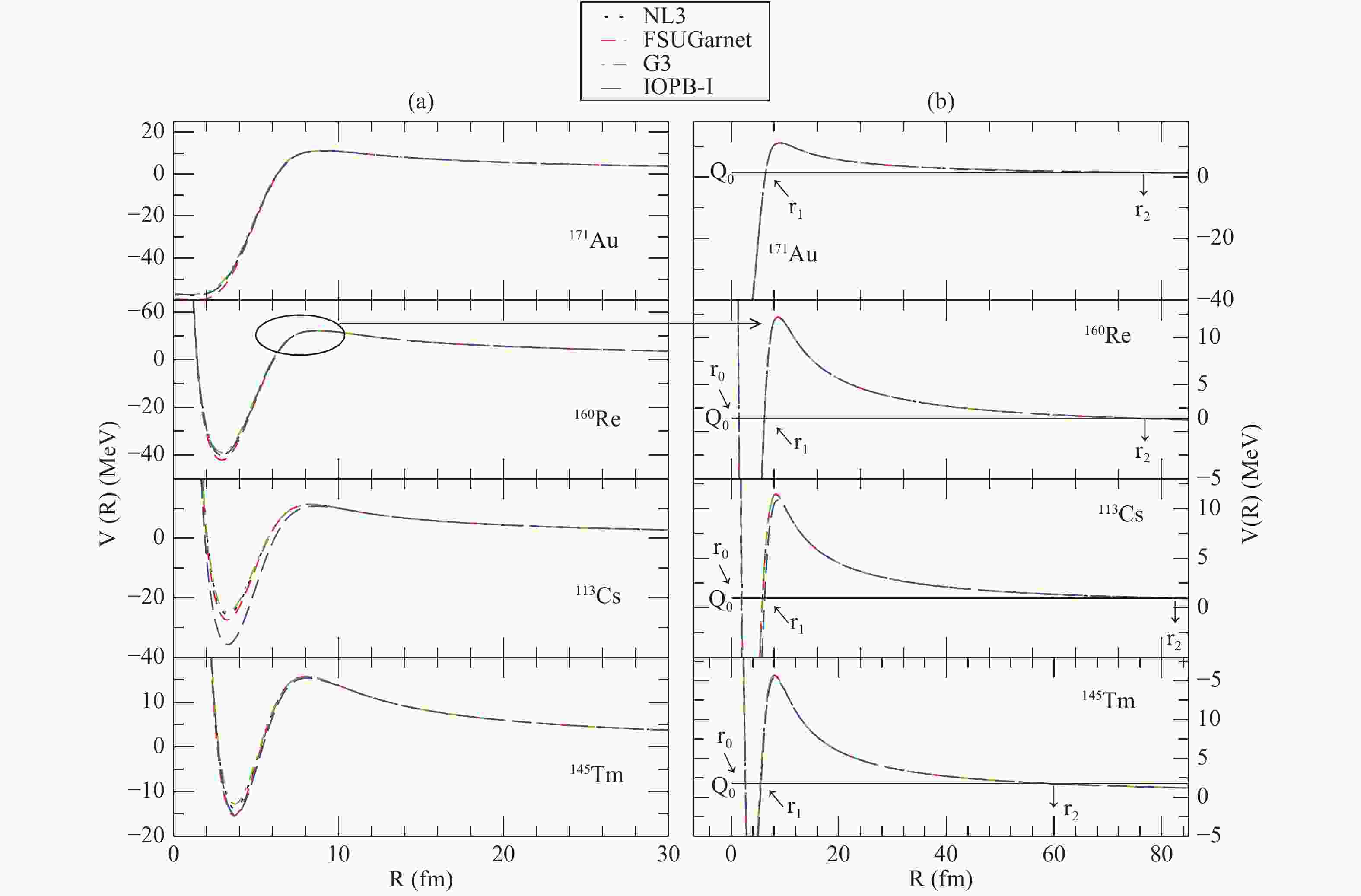
Fig. 1 shows the daughter nucleus-proton optical potential, defined in Eq. (2), for
$ ^{171}{\rm Au} $ ,$ ^{160}{\rm Re} $ ,$ ^{113}{\rm Cs} $ ,$ ^{145}{\rm Tm} $ proton emitters having orbital values of$ \ell $ = 0, 2, 3 and 4, respectively, as determined in this study, which will be discussed in the following subsection. The total effective optical potential is the combination of the nucleus-proton, Coulomb and centrifugal potentials, which have short, long and medium range, respectively. Fig. 1(a) shows the variation of the optical potential as we move away from the center. Due to the absence of the centrifugal potential for$ \ell $ = 0, the potential for$ ^{171}{\rm Au} $ starts from a negative value and then rises towards positive values, whereas all other potentials, for$ \ell $ = 2, 3 and 4 , show the same nature, starting from a high positive value, decreasing towards negative values, and then increasing again to positive values, thus forming a deep potential well. All potential shapes have a hump, which manifests as a potential barrier. The hump portion of Fig. 1(a) is zoomed in Fig. 1(b) in order to show the height of the potential barrier and the turning points more clearly. The black solid straight horizontal line in Fig. 1(b) is the Q value of the decay process. The point where$ Q_{0} $ cuts the$ V(R) $ curve is known as a turning point. For all cases, except$ \ell = 0 $ , we get three turning points marked as$ r_{0}, \; r_{1} $ and$ r_{2} $ . Near the center of the nucleus, the centrifugal potential dominates over the nuclear and Coulomb potentials. Hence, the turning point$ r_{0} $ is mainly due to the centrifugal potential, the turning point$ r_{1} $ is due to the contribution from all three potentials, whereas at the turning point$ r_{2} $ , only the Coulomb and centrifugal potentials are effective as the nuclear potential is negligibly small. The potential for$ \ell = 0 $ yields only two turning points,$ r_{1} $ and$ r_{2} $ . Here, we can say that with increasing$ \ell $ , the oscillation of the interacting particles increases, and hence, we get a larger number of turning points for larger$ \ell $ .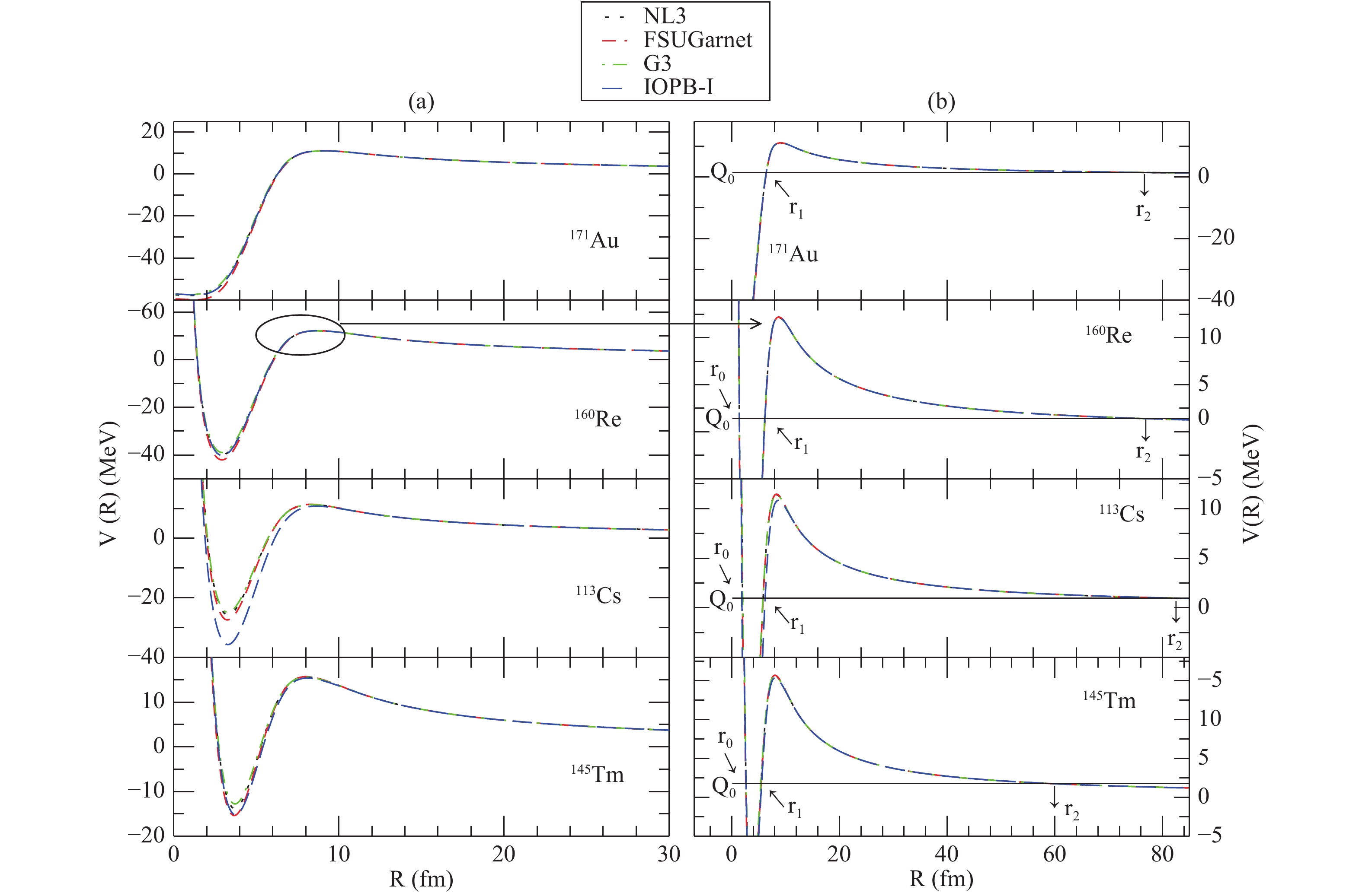
Figure 1. (color online) (a) The total effective optical potential V(R) as a function of radius R. (b) The hump portion of (a) is zoomed in order to show the potential barrier height
$ V_{0} $ and the turning points$ r_{1} $ and$ r_{2} $ for$ ^{171}{\rm Au} $ ,$ ^{160}{\rm Re} $ ,$ ^{113}{\rm Cs} $ and$ ^{145}{\rm Tm} $ nuclei with NL3, FSUGarnet, G3 and IOPB-I interactions in E-RMF.The proton is considered to assault the potential between the turning points
$ r_{1} $ and$ r_{2} $ . The curve from$ r_{1} $ to$ r_{2} $ is defined as the barrier for the emitting particle, and the area under this curve is a measure of the probability of penetration of the effective optical potential. The process of tunneling of the proton through the barrier helps to determine the half-life of a proton emitter. The turning points$ r_{1} $ and$ r_{2} $ and the potential barrier height$ V_{0} $ of the proton emitter using the WKB approximation is noted in Table 2 for all parameter sets considered in this paper.nucleus NL3 FSUGarnet G3 IOPB-I $ r_{1} $ 

$ r_{2} $ 

$ V_{0} $ 

$ r_{1} $ 

$ r_{2} $ 

$ V_{0} $ 

$ r_{1} $ 

$ r_{2} $ 

$ V_{0} $ 

$ r_{1} $ 

$ r_{2} $ 

$ V_{0} $ 

$ ^{109}_{\phantom{1}53}{\rm I} $ 

93.1 6.14 9.40 93.1 6.16 9.42 93.1 6.14 9.37 93.1 6.45 8.79 $ ^{112}_{\phantom{1}55}{\rm Cs} $ 

97.4 6.13 9.65 97.4 6.13 9.71 97.4 6.13 9.62 97.4 6.44 9.18 $ ^{113}_{\phantom{1}55}{\rm Cs} $ 

83.1 5.82 11.38 83.1 5.83 11.45 83.1 5.78 11.35 83.1 6.18 10.83 $ ^{117}_{\phantom{1}57}{\rm La} $ 

98.6 5.79 11.62 98.6 5.82 11.69 98.6 5.77 11.58 98.6 6.36 10.95 $ ^{131}_{\phantom{1}63}{\rm Eu} $ 

94.3 5.77 12.38 94.3 5.78 12.46 94.3 5.78 12.32 94.3 5.98 12.0 $ ^{140}_{\phantom{1}67}{\rm Ho} $ 

86.75 5.79 12.91 86.75 5.82 12.98 86.75 5.72 12.84 86.75 5.92 12.67 $ ^{141}_{\phantom{1}67}{\rm Ho} $ 

84.7 5.82 12.88 84.7 5.84 12.95 84.7 5.80 12.81 84.7 5.95 12.65 $ ^{144}_{\phantom{1}69}{\rm Tm} $ 

60.6 5.40 15.68 60.6 5.45 15.75 60.6 5.37 15.62 60.6 5.53 15.45 $ ^{145}_{\phantom{1}69}{\rm Tm} $ 

59.68 5.43 15.65 59.7 5.45 15.71 59.7 5.36 15.62 59.68 5.55 15.39 $ ^{146}_{\phantom{1}69}{\rm Tm} $ 

104.9 6.44 9.79 105.1 6.45 9.84 105.1 6.43 9.75 105.1 6.49 9.63 $ ^{147}_{\phantom{1}69}{\rm Tm} $ 

96.8 5.36 15.56 96.8 5.45 15.62 96.8 5.35 15.54 96.8 5.53 15.31 $ ^{150}_{\phantom{1}71}{\rm Lu} $ 

77.4 5.43 15.85 77.4 5.46 15.89 77.4 5.35 15.84 77.4 5.52 15.63 $ ^{151}_{\phantom{1}71}{\rm Lu} $ 

84.8 5.42 15.81 84.8 5.46 15.85 84.8 5.35 15.82 84.8 5.51 15.60 $ ^{155}_{\phantom{1}73}{\rm Ta} $ 

75.4 6.33 10.83 75.4 6.36 10.89 75.4 6.33 10.79 75.4 6.39 10.67 $ ^{156}_{\phantom{1}73}{\rm Ta} $ 

95.1 5.84 13.62 95.1 5.86 13.70 95.10 5.81 13.59 95.1 5.89 13.44 $ ^{157}_{\phantom{1}73}{\rm Ta} $ 

111.10 6.42 10.29 111.10 6.45 10.34 111.10 6.39 10.25 111.10 6.47 10.12 $ ^{160}_{\phantom{1}75}{\rm Re} $ 

76.65 6.14 12.15 76.65 6.16 12.20 76.65 6.13 12.13 76.65 6.13 12.20 $ ^{161}_{\phantom{1}75}{\rm Re} $ 

88.6 6.42 10.54 88.6 6.45 10.59 88.6 6.38 10.51 88.6 6.42 10.57 $ ^{164}_{\phantom{1}77}{\rm Ir} $ 

73.25 5.85 14.15 73.25 5.86 14.17 73.25 5.82 14.16 73.25 5.85 14.52 $ ^{165}_{\phantom{1}77}{\rm Ir} $ 

72.7 6.41 10.803 72.7 6.45 10.84 72.7 6.40 10.77 72.7 6.42 10.93 $ ^{166}_{\phantom{1}77}{\rm Ir} $ 

97.6 6.40 10.78 97.6 6.43 10.82 97.6 6.36 10.76 97.6 6.41 10.81 $ ^{167}_{\phantom{1}77}{\rm Ir} $ 

102.4 6.39 10.76 102.4 6.44 10.80 102.4 6.36 10.74 102.4 6.40 10.79 $ ^{170}_{\phantom{1}79}{\rm Au} $ 

80.45 6.31 11.05 80.45 6.41 11.10 80.45 6.33 11.03 80.45 6.39 11.08 $ ^{171}_{\phantom{1}79}{\rm Au} $ 

77.6 6.40 11.04 77.6 6.44 11.08 77.6 6.37 11.01 77.6 6.41 11.07 $ ^{176}_{\phantom{1}81}{\rm Tl} $ 

92.0 6.33 11.38 92.0 6.38 11.41 92.0 6.32 11.35 92.0 6.35 11.42 $ ^{177}_{\phantom{1}81}{\rm Tl} $ 

99.4 6.33 11.39 99.4 6.36 11.42 99.4 6.35 11.35 99.4 6.35 11.44 $ ^{185}_{\phantom{1}83}{\rm Bi} $ 

73.7 6.35 11.85 73.7 6.36 11.84 73.7 6.33 11.78 73.7 6.34 11.91 Table 2. The turning points (
$ r_{1} $ and$ r_{2} $ ) and the potential barrier height$ V_{0} $ calculated from the WKB approximation for spherical proton emitters from Z = 53 to 83 and N = 56 to 102 using the parameter sets NL3, FSUGarnet, G3 and IOPB-I. -
In Table 3, the half-lives of proton emitters are calculated using the spherical E-RMF approach for the four sets of parameters and compared with the experimental data [64, 65] and other theoretical studies [16, 18, 21] for Z = 53 to 83 and N = 56 to 102. The experimental Q values are taken from ref. [63]. Our results for all parameter sets show good agreement with the experimental data, as well as with the other theoretical results. A further inspection of the tabulated values reveals that, except for a few cases, the present calculation gives better results than other studies. To improve our understanding, let us consider the case of the PC-PK1 parameter set where, except for three nuclei
$ ^{145}{\rm Tm} $ ,$ ^{150}{\rm Lu} $ and$ ^{176}{\rm Tl} $ , our calculations show better agreement with the experimental data than the PC-PK1 results. However, for elements$ ^{157}{\rm Ta} $ and$ ^{177}{\rm Tl} $ our calculations show a little deviation. The calculated$ {\rm log}T_{1/2} $ for the above two nuclei are positive quantities whereas the experimental data are negative. But, if we consider the$ T_{1/2} $ values, the calculated and experimental results are comparable. For example, for$ ^{157}{\rm Ta} $ ,$ {\rm log}T_{1/2} $ is 0.582, 0.580, 0.613, 0.550, −0.523 sec and the$ T_{1/2} $ values are 3.824, 3.804, 4.103, 3.545, 0.3 sec for NL3, FSUGarnet, G3, IOPB-I and experiment, respectively. From the above, we can say that, although the$ {\rm log}T_{1/2} $ values for calculated and experimental data have different sign, the positive value of$ T_{1/2} $ implies good agreement of our results with the data for the above two elements. For suitable values of the orbital angular momentum$ \ell $ , all four parameter sets give good agreement with the experimental data, The best set of parameters for the study of proton emission can be obtained by calculating the mean deviation from the experimental results. In this sense, the mean deviation of NL3, FSUGarnet, G3 and IOPB-I was found to be 0.0091, 0.0083, 0.0107 and 0.0068, respectively. Hence, the recent parameter set IOPB-I is found to be more efficient than the other parameter sets. For many cases, our$ \ell $ values do not match the$ \ell $ values in the other theoretical studies, shown in column 7. However, instead of focusing on the$ \ell $ values, emphasis should be given to the$ T_{1/2} $ values, which should agree well with the experimental data, and the corresponding orbitals should be taken as suitable for the proton emission to occur. Half-lives range from 0.01 sec to 5.7 sec, as estimated mainly from the orbital angular momentum$ \ell $ and the Q value.parent nuclei $ \ell $ 

$ {\rm{log}}_{10}T_{1/2} $ (s)

$ \ell $ 

$ {\rm{log}}_{10}T_{1/2} $ (s)

Expt. $ {\rm{log}}_{10}T_{1/2} $ 

NL3 FSUGarnet G3 IOPB-I M3Y [18] R3Y [18] PC-PK1 [21] PCM [16] $ ^{109}_{\phantom{1}53}{\rm I} $ 

2 −4.0408 −4.0245 −4.0121 −4.2594 0, 2 * −5.627 −5.897 −4.441 −3.987 $ ^{112}_{\phantom{1}55}{\rm Cs} $ 

2 −3.1708 −3.1622 −3.1733 −3.3773 2 −2.857 −3.555 −3.638 −3.301 $ ^{113}_{\phantom{1}55}{\rm Cs} $ 

3 −4.4984 −4.2479 −4.2217 −4.4984 2 −5.236 −5.803 −5.759 −4.777 $ ^{117}_{\phantom{1}57}{\rm La} $ 

3 −1.7641 −1.7838 −1.7577 −2.1114 2 −1.943 −2.504 −1.628 $ ^{131}_{\phantom{1}63}{\rm Eu} $ 

3 −1.5383 −1.5060 −1.4932 −1.6645 2 −2.097 −2.764 −1.749 $ ^{140}_{\phantom{1}67}{\rm Ho} $ 

3 −2.6923 −2.1697 −2.1775 −2.2611 2 −1.374 −2.132 −2.221 $ ^{141}_{\phantom{1}67}{\rm Ho} $ 

3 −2.5046 −2.5020 −2.5112 −2.5878 3 −2.487 −3.298 −2.387 $ ^{144}_{\phantom{1}69}{\rm Tm} $ 

4 −5.4711 −5.4747 −5.4393 −5.5598 3 −5.315 −5.5686 $ ^{145}_{\phantom{1}69}{\rm Tm} $ 

4 −5.7857 −5.6670 −5.6266 −5.7498 5 −3.415 −4.698 −5.512 −5.170 −5.409 $ ^{146}_{\phantom{1}69}{\rm Tm} $ 

0 −0.8797 −0.8776 −0.882 −0.9479 5 3.384 1.945 −0.887 −1.096 $ ^{147}_{\phantom{1}69}{\rm Tm} $ 

4 0.7644 0.7243 0.7808 0.6372 5 4.191 2.775 0.783 1.095 0.591 $ ^{150}_{\phantom{1}71}{\rm Lu} $ 

4 −2.1927 −2.2074 −2.14770 −2.2769 5 1.754 0.360 −1.053 −0.859 −1.180 $ ^{151}_{\phantom{1}71}{\rm Lu} $ 

4 −0.9312 −0.9486 −0.8823 −1.0160 5 2.089 0.694 −0.753 −0.573 −0.896 $ ^{155}_{\phantom{1}73}{\rm Ta} $ 

1 −4.7255 −4.7285 −4.7259 −4.7627 5 −2.907 −4.238 −2.279 −4.637 −4.921 $ ^{156}_{\phantom{1}73}{\rm Ta} $ 

3 −0.1262 −1.1383 −0.1200 −1.1794 2 −0.138 −0.80 −0.469 −0.461 −0.620 $ ^{157}_{\phantom{1}73}{\rm Ta} $ 

0 0.5824 0.5802 0.6130 0.5496 0 −0.469 −0.982 −0.048 −0.126 −0.523 $ ^{160}_{\phantom{1}75}{\rm Re} $ 

2 −3.7384 −3.7719 −3.7615 −3.7598 2 −2.947 −3.602 −1.0409 −3.109 −3.046 $ ^{161}_{\phantom{1}75}{\rm Re} $ 

0 −2.4666 −2.5718 −2.5301 −2.5599 0 −3.577 −4.089 −3.0731 −3.231 −3.432 $ ^{164}_{\phantom{1}77}{\rm Ir} $ 

3 −3.3824 −3.4087 −3.3649 −3.3584 5 −2.491 −3.780 −4.193 −3.959 $ ^{165}_{\phantom{1}77}{\rm Ir} $ 

0 −5.0386 −5.0556 −5.0046 −5.0386 0 −6.453 −6.848 −6.0 $ ^{166}_{\phantom{1}77}{\rm Ir} $ 

0 −0.8345 −0.8710 −0.8156 −0.8588 2 −0.891 −1.545 −0.976 −1.160 −0.824 $ ^{167}_{\phantom{1}77}{\rm Ir} $ 

0 −0.1153 −0.1519 −0.1412 −0.1392 0 −1.28 −1.798 −0.919 −0.943 −0.959 $ ^{170}_{\phantom{1}79}{\rm Au} $ 

0 −3.4097 −3.4465 −3.3968 −3.4085 2 −3.771 −3.49349 $ ^{171}_{\phantom{1}79}{\rm Au} $ 

0 −3.9480 −3.9539 −3.9064 −3.3944 0 −5.122 −5.641 −4.581 −4.794 −4.770 $ ^{176}_{\phantom{1}81}{\rm Tl} $ 

0 −1.1813 −1.1932 −1.1784 −1.1781 0 −2.058 −2.2839 $ ^{177}_{\phantom{1}81}{\rm Tl} $ 

0 0.01315 −0.0209 0.01350 0.0167 0 −1.364 −1.925 −0.786 −0.993 −1.174 $ ^{185}_{\phantom{1}83}{\rm Bi} $ 

0 −4.1324 −4.1450 −4.1363 −4.1271 0 −5.557 −6.179 −5.237 −5.184 −4.229 * $ \ell $ = 0, 2 corresponds to the results from [18] and [21] respectively.

Table 3. The logarithmic half-lives of proton emitters in their ground state for the parameter sets NL3 [43], FSUGarnet [44], G3 [24] and IOPB-I [45]. The experimental Q values are taken from Ref. [63]. Our results are compared with the experimental data taken from ref. [64, 65] and with the results of [16, 18, 21].
$ \ell $ represents the orbital angular momentum of the emitting proton.The sensitivity of the half-life to the
$ \ell $ values is shown in Fig. 2 for$ ^{171}{\rm Au} $ ,$ ^{160}{\rm Re} $ ,$ ^{113}{\rm Cs} $ and$ ^{145}{\rm Tm} $ , as representative cases. For all parameter sets, as the value of$ \ell $ increases the life-time of the proton emitter increases. This gives a clue that a proton from the$ \ell = 0 $ orbit has a larger probability for emission. But, due to many other nuclear properties, such as the proton separation energy, chemical potential, depth of the potential well etc., the outgoing proton is emitted from the orbit most favorable for all nuclear properties. Hence, we may get optimistic information on the shell structure of the proton emitter. In Fig. 2, unfilled symbols are the theoretical results and the solid symbols are the experimental data. For nuclei$ ^{171}{\rm Au} $ and$ ^{160}{\rm Re} $ , with reported$ \ell $ values of$ \ell = 0, 2 $ , respectively, the experimental and theoretical values show good agreement. For nuclei$ ^{113}{\rm Cs} $ and$ ^{145}{\rm Tm} $ , the experimental half-lives are shown for two$ \ell $ values, one for the$ \ell $ value reported in the previous works [15-18, 21], and the other for the$ \ell $ value reported in the present study. The square symbols with a red line (online) show the variation of the logarithmic half-life ($ {\rm log}T_{1/2} $ ) with$ \ell $ for$ ^{145}{\rm Tm} $ . The experimental value of$ {\rm log}T_{1/2} $ is represented by filled squares. We found that the half-life for the estimated value of the orbital angular momentum in this study, i.e.$ \ell = 4 $ , shows better agreement than$ \ell = 5 $ , reported in previous works. Similarly, circle symbols with a black line (online) show the variation of$ {\rm log}T_{1/2} $ with$ \ell $ for$ ^{113}{\rm Cs} $ . The values$ \ell $ = 2 and 3 are respectively for the previous and present works. Here, however, the experimental half-lives are closer to the calculated results for both$ \ell $ = 2 and 3.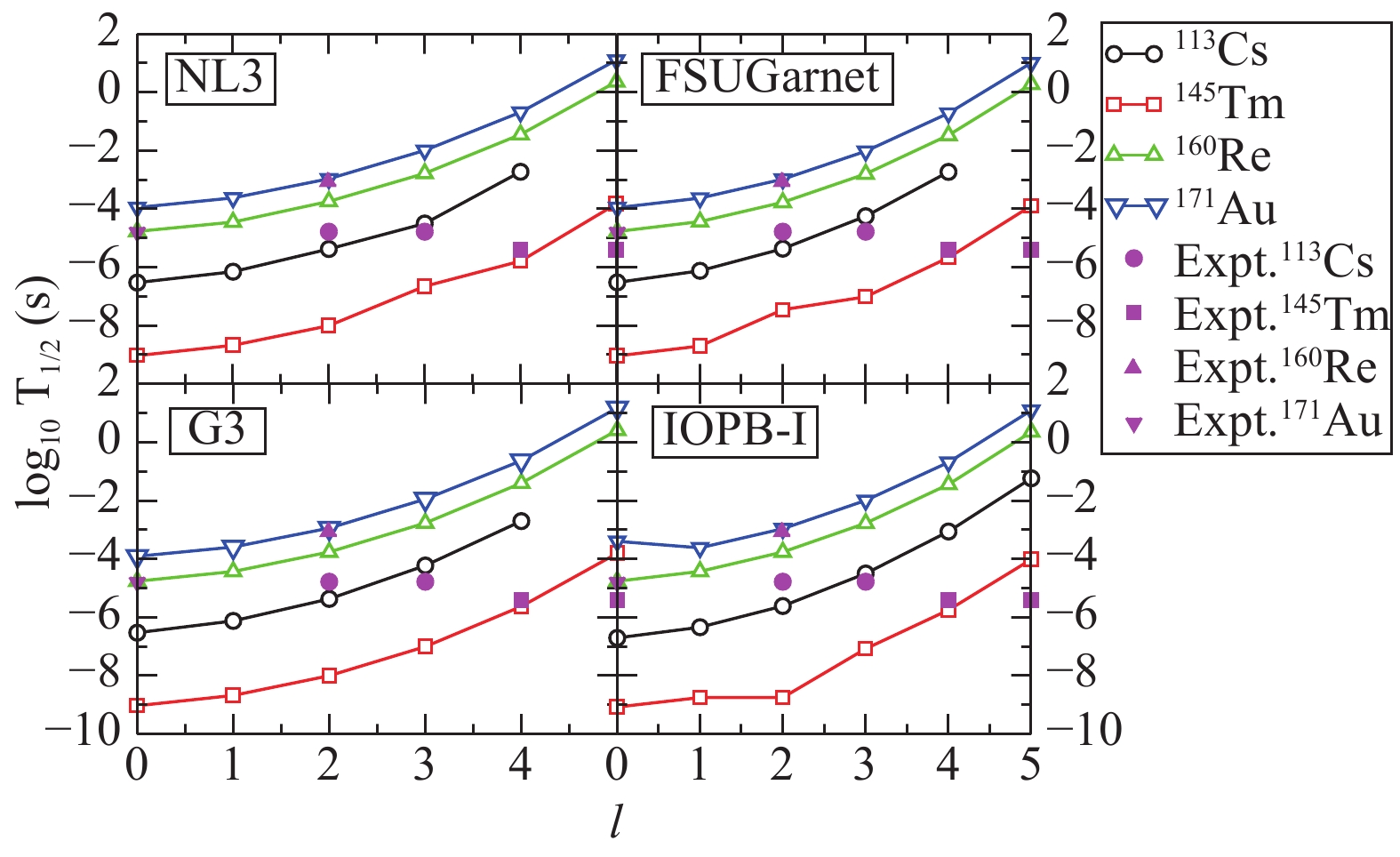
Figure 2. (color online) The sensitivity of the logarithmic half-life to the orbital angular momentum
$ \ell $ for$ ^{171}{\rm Au} $ ,$ ^{160}{\rm Re} $ ,$ ^{113}{\rm Cs} $ ,$ ^{145}{\rm Tm} $ nuclei with NL3, FSUGarnet, G3 and IOPB-I interactions in E-RMF.The agreement of the calculated and experimental half-lives is more clearly seen in Fig. 3, where the ratio of the calculated half-live
$ \left({\rm log}T{^{\rm cal}_{1/2}}\right) $ to the experimental one$ \left({\rm log}T{^{\rm exp}_{1/2}} \right) $ is shown as a function of the mass number A. We observe that the maximum points are around$ \displaystyle\frac{{\rm log}T{^{\rm cal}_{1/2}}}{{\rm log}T{^{\rm exp}_{1/2}}} \approx 1 $ , which illustrates the high degree of agreement between the experimental data and the theoretical results. However, there are some data points which deviate from this line, among which$ ^{157}{\rm Ta} $ , which has a maximum deviation, as can also be seen in Table 3. The reason behind the deviation is that we have assumed that all proton emitters are spherical in shape, which may not exactly be the case, as some of them are in reality moderately deformed.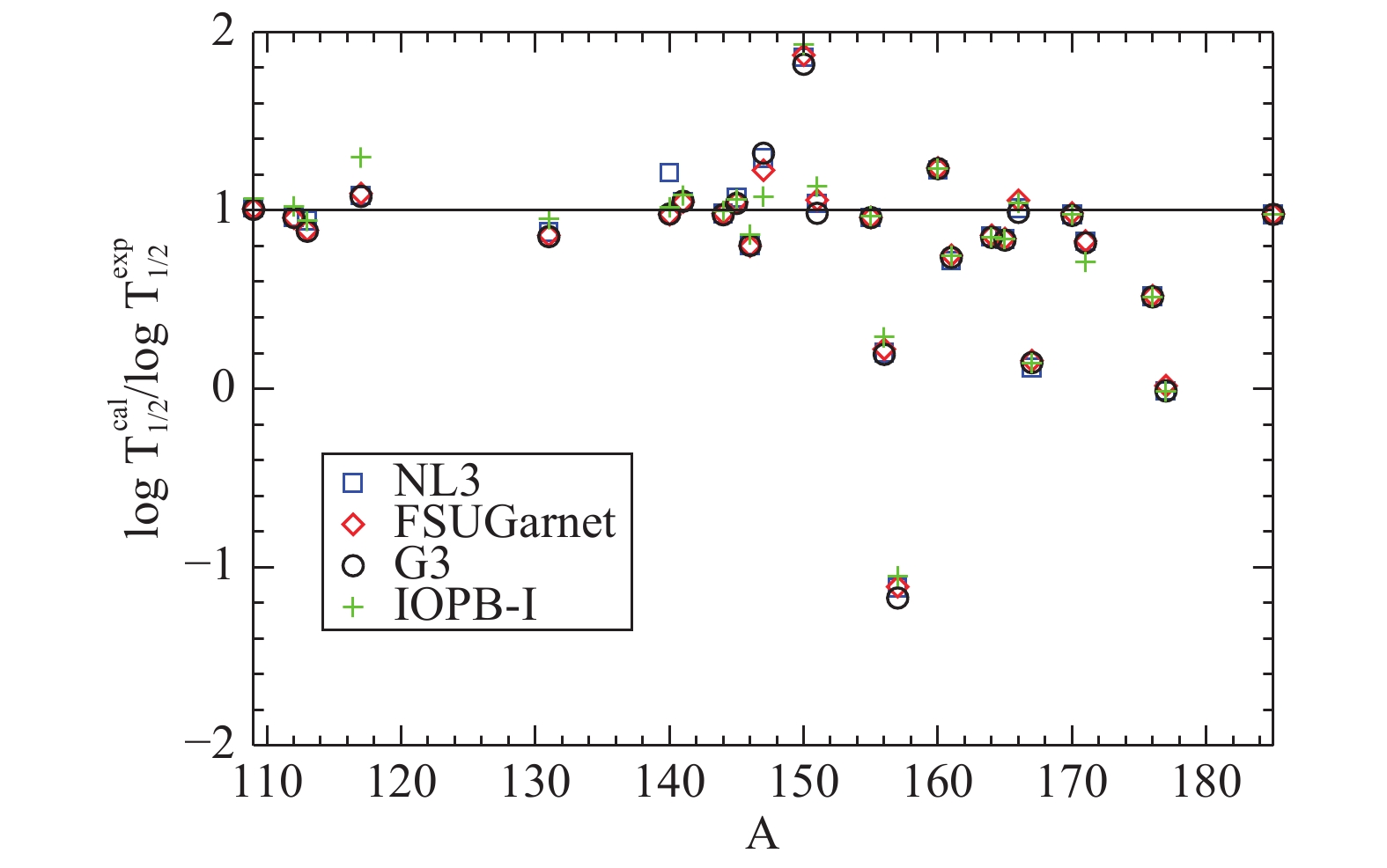
Figure 3. (color online) Ratio of the calculated to the experimental half-life
$ \left(\displaystyle\frac{{\rm log}T{^{\rm cal}_{1/2}}}{{\rm log}T{^{\rm exp}_{1/2}}} \right)$ as a function of the mass number A for proton emitters from Z = 53 to 83 and N = 56 to 102 using NL3, FSUGarnet, G3 and IOPB-I interactions in E-RMF.Summarizing briefly the above results, we found that the considered proton emitters lie around the maximum of the curve of the binding energy per nucleon B/A. Due to the insufficient number of neutrons, the proportionality between protons and neutrons breaks down, and a proton gets emitted. From the asymmetrical distribution of protons and neutrons, the radial distribution of protons (
$ r_{p} $ ) is found to be greater than the radial distribution of neutrons ($ r_{n} $ ), but due to the small thickness of aggregated protons in the outer part of the nucleus, we cannot call it a proton skin. The outer protons feel the repulsive Coulomb force, as well as the singlet-singlet or triplet-triplet repulsive proton-proton nuclear force. Also, due to the decrease in the strength of the binding energy for outer orbitals, these protons are found to be loosely bound. Therefore, they undergo emission.The proton decay process was studied using the WKB barrier penetration method. We found that the potential is highly sensitive to the orbital angular momentum
$ \ell $ . With an increase of$ \ell $ the half-life also increases. Hence, the reported values of$ \ell $ are chosen such that the calculated half-life agrees with the experimental data. Our calculated results show good agreement with the experimental data [64, 65] and other theoretical studies [16, 18, 21]. -
Summarizing the context, we studied the nuclear properties of proton emitters from I to Bi with Z = 53 to 83 and N = 56 to 102 in their ground state based on the spherical effective relativistic mean-field (E-RMF) formalism with NL3, FSUGarnet, G3 and IOPB-I interactions. The binding energy per nucleon B/A tells us about the strength of binding between nucleons, which is found to be maximum around the iron peak in the general B/A curve. For the stable configuration of the nucleus, more neutrons are required than protons in order to compensate the repulsive Coulomb and singlet-singlet or triplet-triplet repulsive nuclear force. Due to inadequate number of neutrons, the shape harmony between protons and neutrons breaks down, making the nucleus unstable. The negative value of the neutron skin thickness (
$ \Delta r_{n} = r_{n}-r_{p} $ ) indicates that the radial distribution of protons ($ r_{p} $ ) is greater than that of neutrons ($ r_{n} $ ). For the compensation of Coulomb force between protons, all neutrons are accommodated among protons forming the tightly bound singlet-triplet attractive np-core. The remaining loosely bound protons, which are not involved in the compensation process, remain in the outer surface of the nucleus and can readily undergo emission. These protons form a very thin layer on the surface of the nucleus. Due to the small thickness of this layer it will be fallacious to say that it is a proton skin. The experimental Q values [63] are taken for calculating the proton decay half-life using the WKB method, where the effective potential is constructed by adding the contributions from the nuclear, Coulomb and centrifugal potentials. For the nuclear potential, we have used the double folding model with the realistic M3Y nucleon-nucleon interaction. The results for the half-life for all four interactions (NL3, FSUGarnet, G3 and IOPB-I) with the above approach show very good agreement with the experimental data. Except in a few cases, our study gives better results than other theoretical studies [16, 18, 21]. It was noted that, on average, the half-lives of proton emitters are highly susceptible to the orbital angular momentum ($ \ell $ ) carried by the emitted proton. An increase of the$ \ell $ value increases the half-life$ {\rm log}T_{1/2} $ . However, the emission of a proton occurs from the orbital which is favorable from all points of view, including B/A, charge distribution, proton separation energy, chemical potential, etc. The$ \ell $ values reported in our work are chosen such that the calculated half-lives agree with the experimental ones. Hence, our study helps to position the boundary of the nuclear landscape on the proton side. It also helps to analyze the shell structure of the proton rich nuclei and collect valuable information on the nuclear forces in the drip-line region. Moreover, the emission of a proton from the ground state gives a hindrance for the existence of more exotic nuclei.The authors thank Dr. Bharat Kumar for fruitful discussions and acknowledge Institute of Physics (IOP), Bhubaneswar for providing the necessary computer facilities.
Proton emission from the drip-line nuclei I-Bi using the WKB approximation with relativistic mean-field densities
- Received Date: 2018-11-13
- Available Online: 2019-04-01
Abstract: We study the properties of proton rich nuclei reported as proton emitters in the region from I to Bi with Z = 53 to 83 and N = 56 to 102 as a crucial application to the existence of exotic nuclei. The effective relativistic mean-field formalism (E-RMF), with NL3, FSUGarnet, G3 and IOPB-I interactions, is adopted for analysis of the ground state properties of proton emitters. Furthermore, in the E-RMF background, the Wentzel-Karmers-Brillouin (WKB) barrier penetration method is used for the calculation of proton emission half-lives. It is found that the calculated half-lives are in good agreement with the experimental results for all emitters considered in this study.


 DownLoad: