


 Abstract
 HTML
HTML Reference
 Related
 PDF
PDF


-
Rare decays are of a great importance in studying New Physics (NP) beyond the Standard Model (SM); in particular, the lepton-flavor-violation (LFV) decays are appealing because they are suppressed in the SM, and their detection would be a manifest signal of NP. The search for such LFV decays has been pursued to date in a host of processes of leptons, Z boson, Higgs boson, and various hadrons. The present upper bounds on the various LFV decay channels of Z boson from both the LEP data and LHC data is summarized in Table 1 [1]. A pedagogical introduction on the theoretical motivations for charged LFV and the experimental aspects is provided in Ref. [6].
decay bound experiment bound experiment $Z\rightarrow e\mu$ 

$1.7\times 10^{-6}$ 

LEP (1995) [2] $7.5\times 10^{-7}$ 

ATLAS (2014) [3] $Z\rightarrow e\tau$ 

$9.8\times 10^{-6}$ 

LEP (1995) [2] $5.8\times 10^{-5}$ 

ATLAS (2018) [4] $Z\rightarrow \mu\tau$ 

$1.2\times 10^{-5}$ 

LEP (1995) [5] $1.3\times 10^{-5}$ 

ATLAS (2018) [4] Table 1. Current limits on LFV decays of Z boson.
As a new solution to the supersymmetric flavor problem in MSSM, the minimal R-symmetric supersymmetric SM (MRSSM) is proposed in Ref. [7], where the R-symmetry is a fundamental symmetry, which was proposed several decades ago, and is stronger than the R-parity [8, 9]. R-symmetry forbids Majorana gaugino masses,
$ \mu $ term, A terms, and all left-right squark and slepton mass mixings. The R-charged Higgs$ SU(2)_L $ doublets$ \hat{R}_u $ and$ \hat{R}_d $ are introduced in the MRSSM to yield the Dirac mass terms of higgsinos. Additional superfields$ \hat{S} $ ,$ \hat{T} $ and$ \hat{O} $ are introduced to yield Dirac mass terms of gauginos. Studies on phenomenology in MRSSM can be found in literature [10-23].In this study, we investigated the LFV decays of Z boson in MRSSM. Similar to the case in MSSM, the LFV decays mainly originate from the off-diagonal entries in slepton mass matrices
$ m_l^2 $ and$ m_r^2 $ [24]. Considering the constraint from radiative decay$ l_2\rightarrow l_1\gamma $ on the off-diagonal parameters, we give the upper predictions on the LFV decays of Z boson with parameter spaces BMP1 and BMP3 [12]. Further, considering recent experimental limit on the masses of charginos and neutrilinos [25], we explore the LFV decays of Z boson as a function of Dirac mass parameter$ M_D^W $ . A comparison of the upper bounds of the off-diagonal parameters of the MRSSM and the MSSM is also presented.The remainder of this paper is organized as follows. In Section 2, we provide a brief introduction on the MRSSM, and we derive the analytic expressions for every Feynman diagram contributing to the LFV decays of Z boson in the MRSSM in detail. The numerical results are presented in Section 3, and the conclusion is provided in Section 4.
-
In this section, we first provide a simple overview of the MRSSM. The spectrum of fields in the MRSSM contain the standard MSSM matter; Higgs and gauge superfields augmented by chiral adjoints
$ \hat{\cal O},\hat{T},\hat{S} $ ; and two R-Higgs iso-doublets. The superfields with R-charge in the MRSSM are listed in Table 2. The general form of the superpotential of the MRSSM is given by [10]field superfield boson fermion gauge vector $ \hat{g},\hat{W},\hat{B} $ 

0 $ g,W,B $ 

0 $ \tilde{g},\tilde{W}\tilde{B} $ 

+1 matter $ \hat{l}, \hat{e}^c $ 

+1 $ \tilde{l},\tilde{e}^*_R $ 

+1 $ l,e^*_R $ 

0 $ \hat{q},{\hat{d}^c},{\hat{u}^c} $ 

+1 $ \tilde{q},{\tilde{d}}^*_R,{\tilde{u}}^*_R $ 

+1 $ q,d^*_R,u^*_R $ 

0 $ H $ -Higgs

$ {\hat{H}}_{d,u} $ 

0 $ H_{d,u} $ 

0 $ {\tilde{H}}_{d,u} $ 

−1 R-Higgs $ {\hat{R}}_{d,u} $ 

+2 $ R_{d,u} $ 

+2 $ {\tilde{R}}_{d,u} $ 

+1 adjoint chiral $ \hat{\cal O},\hat{T},\hat{S} $ 

0 $ O,T,S $ 

0 $ \tilde{O},\tilde{T},\tilde{S} $ 

−1 Table 2. Superfields with R-charge in MRSSM.
$\begin{split} {{\cal W}_{\rm MRSSM}} =& {\mu _d}\left({{\hat R}_d}{{\hat H}_d}\right) + {\mu _u}\left({{\hat R}_u}{{\hat H}_u}\right) \\&+ {\Lambda _d}\left({{\hat R}_d}\hat T\right){{\hat H}_d} + {\Lambda _u}\left({{\hat R}_u}\hat T\right){{\hat H}_u}\\& + {\lambda _d}\hat S\left({{\hat R}_d}{{\hat H}_d}\right) + {\lambda _u}\hat S\left({{\hat R}_u}{{\hat H}_u}\right) \\&- {Y_d}\hat d\left(\hat q{{\hat H}_d}\right) - {Y_e}\hat e\left(\hat l{{\hat H}_d}\right) + {Y_u}\hat u\left(\hat q{{\hat H}_u}\right), \end{split}$

(1) where
$ \hat{H}_u $ and$ \hat{H}_d $ are the MSSM-like Higgs weak iso-doublets;$ \hat{R}_u $ and$ \hat{R}_d $ are the R-charged Higgs$ SU(2)_L $ doublets and the corresponding Dirac higgsino mass parameters are denoted as$ \mu_u $ ; and$ \mu_d $ .$ \lambda_u $ ,$ \lambda_d $ ,$ \Lambda_u $ and$ \Lambda_d $ are parameters of Yukawa-like trilinear terms involving the singlet$ \hat{S} $ and the triplet$ \hat{T} $ , which is given by$\hat T = \left( {\begin{array}{*{20}{c}} {{{\hat T}^0}/\sqrt 2 }&{{{\hat T}^ + }}\\ {{{\hat T}^ - }}&{ - {{\hat T}^0}/\sqrt 2 } \end{array}} \right).$

Then, the soft-breaking terms involving the scalar mass are
$\begin{split} {V_{SB,S}} =& m_{{H_d}}^2\left(|H_d^0{|^2} + |H_d^ - {|^2}\right) + m_{{H_u}}^2\left(|H_u^0{|^2} + |H_u^ + {|^2}\right) \\&+ \left({B_\mu }\left(H_d^ - H_u^ + - H_d^0H_u^0\right) + h.c.\right) + m_{{R_d}}^2\left(|R_d^0{|^2} + |R_d^ + {|^2}\right) \\&+ m_{{R_u}}^2\left(|R_u^0{|^2} + |R_u^ - {|^2}\right) + m_T^2\left(|{T^0}{|^2} + |{T^ - }{|^2} + |{T^ + }{|^2}\right) \\&+ m_S^2|S{|^2}\!\! + m_O^2|{O^2}| + \tilde d_{L,i}^*m_{q,ij}^2{{\tilde d}_{L,j}} + \tilde d_{R,i}^*m_{d,ij}^2{{\tilde d}_{R,j}} \\&+ \tilde u_{L,i}^*m_{q,ij}^2{{\tilde u}_{L,j}} + \tilde u_{R,i}^*m_{u,ij}^2{{\tilde u}_{R,j}} + \tilde e_{L,i}^*m_{l,ij}^2{{\tilde e}_{L,j}} \\&+ \tilde e_{R,i}^*m_{r,ij}^2{{\tilde e}_{R,j}} + \tilde \nu _{L,i}^*m_{l,ij}^2{{\tilde \nu }_{L,j}}. \end{split}$

(2) Note that all trilinear scalar couplings of Higgs bosons, squarks, sleptons, etc. are forbidden owing to the R-symmetry. The Dirac nature is a manifest feature of the MRSSM fermions, and the soft-breaking Dirac mass terms of the singlet
$ \hat{S} $ , triplet$ \hat{T} $ , and octet$ \hat{O} $ take the form${V_{SB,DG}} = M_D^B\tilde B\tilde S + M_D^W{\tilde W^a}{\tilde T^a} + M_D^O\tilde g\tilde O + {\rm h.c.},$

(3) where
$ \tilde{B} $ ,$ \tilde{W} $ , and$ \tilde{g} $ are usually MSSM Weyl fermions. After EWSB, one can get the following$ 4\times 4 $ neutralino mass matrix${m_{{\chi ^0}}} = \left( {\begin{array}{*{20}{c}} {M_D^B}&0&{ - \displaystyle\frac{1}{2}{g_1}{v_d}}&{\displaystyle\frac{1}{2}{g_1}{v_u}}\\ 0&{M_D^W}&{\displaystyle\frac{1}{2}{g_2}{v_d}}&{ - \displaystyle\frac{1}{2}{g_2}{v_u}}\\ { - \displaystyle\frac{1}{{\sqrt 2 }}{\lambda _d}{v_d}}&{ - \displaystyle\frac{1}{2}{\Lambda _d}{v_d}}&{ - \mu _d^{\rm eff, + }}&0\\ {\displaystyle\frac{1}{{\sqrt 2 }}{\lambda _u}{v_u}}&{ - \displaystyle\frac{1}{2}{\Lambda _u}{v_u}}&0&{\mu _u^{\rm eff, - }} \end{array}} \right),$

(4) where the modified
$ \mu_i $ parameters are$\begin{split} {\mu _d^{\rm eff, + }}&{ = \displaystyle\frac{1}{2}{\Lambda _d}{v_T} + \frac{1}{{\sqrt 2 }}{\lambda _d}{v_S} + {\mu _d},}\\ {\mu _u^{\rm eff, - }}&{ = - \displaystyle\frac{1}{2}{\Lambda _u}{v_T} + \frac{1}{{\sqrt 2 }}{\lambda _u}{v_S} + {\mu _u},} \end{split}$

and
$ v_T $ and$ v_S $ are vacuum expectation values of$ \hat{T} $ and$ \hat{S} $ , respectively, which carry zero R-charge.The neutralino mass matrix can be diagonalized by unitary matrices
$ N^1 $ and$ N^2 $ ${({N^1})^ * }{m_{{\chi ^0}}}{({N^2})^†} = {\rm diag}({m_{\chi _1^0}},...,{m_{\chi _4^0}}).$

The chargino mass matrix is given by
${m_{{\chi ^ \pm }}} = \left( {\begin{split} {{g_2}{v_T} + M_D^W}&{\displaystyle\frac{1}{{\sqrt 2 }}{\Lambda _d}{v_d}}\\ {\displaystyle\frac{1}{{\sqrt 2 }}{g_2}{v_d}}&{ - \displaystyle\frac{1}{2}{\Lambda _d}{v_T} + \displaystyle\frac{1}{{\sqrt 2 }}{\lambda _d}{v_S} + {\mu _d}} \end{split}} \right),$

(5) and it can be diagonalized by unitary matrices
$ U^1 $ and$ V^1 $ ${({U^1})^ * }{m_{{\chi ^ \pm }}}{({V^1})^†} = {\rm diag}({m_{\chi _1^ \pm }},{m_{\chi _2^ \pm }}).$

The LFV interactions are mainly caused by the potential misalignment between the leptons and the sleptons mass matrices in the MRSSM. In the gauge eigenstate basis
$ \tilde{\nu}_{iL} $ , the sneutrino mass squared matrix is expressed as$\begin{split} m_{\tilde \nu }^2 = {m_l^2 + \displaystyle\frac{1}{8}(g_1^2 + g_2^2)(v_d^2 - v_u^2) + {g_2}{v_T}M_D^W - {g_1}{v_S}M_D^B,} \end{split}$

(6) where the last two terms are newly introduced by the MRSSM, and the mass matrix is diagonalized by the unitary matrix
$ Z^V $ ${Z^V}m_{\tilde \nu }^2{({Z^V})^†} = {\rm diag}(m_{{{\tilde \nu }_1}}^2,m_{{{\tilde \nu }_2}}^2,m_{{{\tilde \nu }_3}}^2).$

The slepton mass squared matrix can be expressed as
$m_{{{\tilde L}^ \pm }}^2 = \left( {\begin{array}{*{20}{c}} {{{(m_{{{\tilde L}^ \pm }}^2)}_{LL}}}&0\\ 0&{{{(m_{{{\tilde L}^ \pm }}^2)}_{RR}}} \end{array}} \right),$

(7) where
$\begin{gathered} {\left( {m_{{{\tilde L}^ \pm }}^2} \right)_{LL}} = m_l^2 + \frac{1}{2}v_d^2|{Y_e}{|^2} + \frac{1}{8}\left( {g_1^2 - g_2^2} \right)\left( {v_d^2 - v_u^2} \right) \\ - {g_1}{v_S}M_D^B - {g_2}{v_T}M_D^W, \\ {\left( {m_{{{\tilde L}^ \pm }}^2} \right)_{RR}} = m_r^2 + \frac{{v_d^2}}{2}|{Y_e}{|^2} + \frac{1}{4}g_1^2\left( {v_u^2 - v_d^2} \right) + 2{g_1}{v_S}M_D^B. \end{gathered} $

The sources of the LFV are the off-diagonal entries of the 3×3 soft supersymmetry breaking matrices
$ m_l^2 $ and$ m_r^2 $ , where the A terms are absent. Note that, in the following, we replace$ \tilde{l} $ with$ \tilde{L}^{\pm} $ to denote the sleptons. From Eq. (7), we can see that the left-right slepton mass mixing is also absent. The slepton mass matrix is diagonalized by the unitary matrix$ Z^E $ ${Z^E}m_{{{\tilde L}^ \pm }}^2{\left({Z^E}\right)^†} = {\rm diag}\left(m_{\tilde L_1^ \pm }^2,...,m_{\tilde L_6^ \pm }^2\right).$

The interactions of the charged sleptons
$ \tilde{L}^{\pm} $ and neutral sneutrinos$ \tilde{\nu} $ with neutralinos$ \chi^0 $ and charginos$ \chi^{\pm} $ are correspondingly given by the Lagrangian as [12, 26]$\begin{split} - i{\cal L} =& \bar \chi _i^0\left[Y_e^{{l_j}}N_{i3}^{2 * }Z_{k\left(3 + j\right)}^E{P_L} + \sqrt 2 {g_1}Z_{k\left(3 + j\right)}^EN_{i1}^1{P_R}\right]{l_j}\tilde L_k^ \pm \\&+ {{\bar \chi }^ \pm }\left[{g_2}V_{i1}^{1 * }Z_{kj}^V{P_L} - Z_{kj}^VU_{i2}^1{P_R}\right]{l_j}{{\tilde \nu }_k}. \end{split}$

The interactions between Z boson and neutralinos
$ \chi^0 $ or charginos$ \chi^{\pm} $ are given by the Lagrangian as$\begin{split} - i{\cal L} =& \frac{1}{2}\bar \chi _i^ \pm {\gamma _\mu }[\left(2{g_2}{c_w}V_{j1}^{1 * }V_{i1}^1 + \left({g_2}{c_w} - {g_1}{s_w}\right)V_{j2}^{1 * }V_{i2}^1\right){P_L} \\&+ \left(\left({g_2}{c_w} - {g_1}{s_w}\right)U_{i2}^{1 * }U_{j2}^1 + 2{g_2}{c_w}U_{i1}^{1 * }U_{j2}^1\right){P_R}]\tilde \chi _j^ \pm {Z^\mu } \\&+ \frac{1}{2}\left({g_1}{s_w} + {g_2}{c_w}\right)\bar \chi _i^0{\gamma _\mu }[\left(N_{j4}^{1 * }N_{i4}^1 - N_{j3}^{1 * }N_{i3}^1\right){P_L} \\&+ \left(N_{i4}^{2 * }N_{j4}^2 - N_{i3}^{2 * }N_{j3}^2\right){P_R}]\chi _j^0{Z^\mu }. \end{split}$

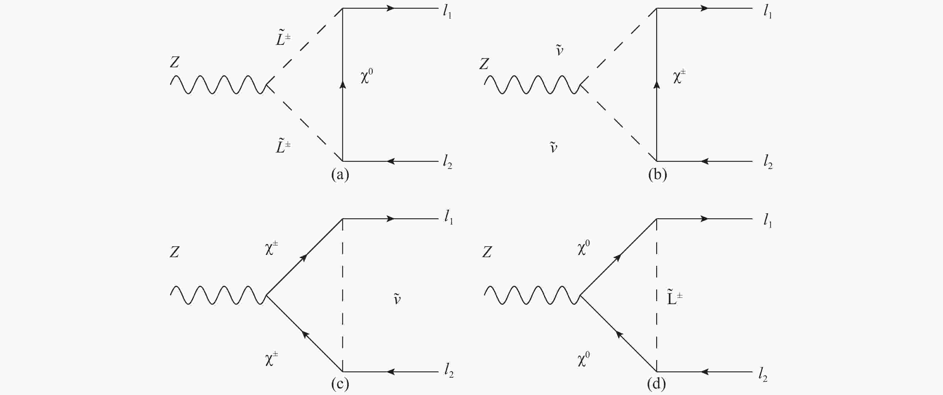
The relevant Feynman diagrams contributing to the LFV decays of Z boson in the MRSSM is presented in Fig. 1, where Fig. 1(a) and Fig. 1(c) take more important role than others. The
$ Z l_1l_2 $ interaction Lagrangian can be written as [27]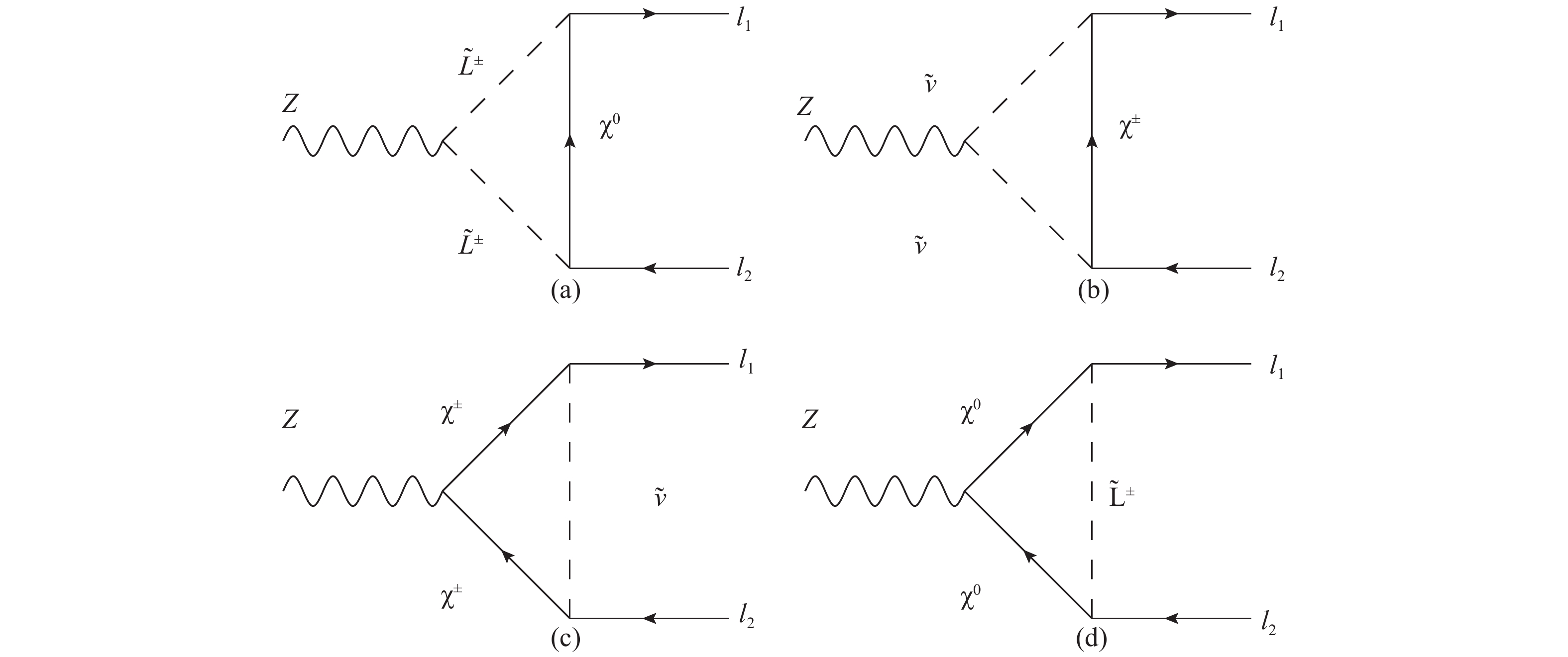
Figure 1. One loop Feynman diagrams contributing to
$ Z\rightarrow \bar{l}_1l_2 $ in MRSSM.${{\cal L}_{Z{l_1}{l_2}}} = {\bar l_1}[{\gamma ^\mu }(C_L^1{P_L} + C_R^1{P_R}) + p_1^\mu (C_L^2{P_L} + C_R^2{P_R})]{l_2}{Z_\mu }.$

(8) The left-handed current coefficient
$ C^1_L $ for Fig. 1(a) and the right-handed current coefficient$ C^1_R $ for Fig. 1(c) are dominant in the final result. Then the branching ratios of LFV decays of Z boson are calculated using$\begin{split} {\rm Br}(Z \to {l_1}{l_2}) =& {\rm Br}(Z \to {{\bar l}_1}{l_2}) + {\rm Br}(Z \to {{\bar l}_2}{l_1})\\ = & \displaystyle\frac{{{m_Z}}}{{48\pi {\Gamma _Z}}}[2(|C_L^1{|^2} + |C_R^1{|^2}) + \displaystyle\frac{{m_Z^2}}{4}(|C_L^2{|^2} + |C_R^2{|^2})], \end{split}$

(9) where the charged lepton masses have been neglected, and
$ \Gamma_Z $ is the total decay width of Z boson. The coefficients$ C^{1}_{L/R} $ and$ C^{2}_{L/R} $ are combinations of coefficients corresponding to each Feynman diagram in Fig. 1 and can be expressed as$\begin{array}{l} C_{L/R}^1 = C_{L/R}^{1,a} + C_{L/R}^{1,b} + C_{L/R}^{1,c} + C_{L/R}^{1,d},\\ C_{L/R}^2 = C_{L/R}^{2,a} + C_{L/R}^{2,b} + C_{L/R}^{2,c} + C_{L/R}^{2,d}. \end{array}$

The coefficients in Fig. 1(a) and Fig. 1(b) can be written as
$\begin{split} C_L^{1,a/b} =& 2{C_{1R}}{C_2}{C_{3L}}{{\cal C}_{00}},C_R^{1,a/b} = 2{C_{1L}}{C_2}{C_{3R}}{{\cal C}_{00}},\\ C_L^{2,a/b} =& 2{C_2}({C_{1L}}({C_{3R}}{m_2} \!-\! {C_{3L}}{M_3}){{\cal C}_2} \!-\! {C_{1L}}{C_{3L}}{M_3}{{\cal C}_0} \\&\!-\! {C_{1L}}{C_{3L}}{M_3}{{\cal C}_1} + {C_{1L}}{C_{3R}}{m_2}{{\cal C}_{22}} + {C_{1L}}{C_{3R}}{m_2}{{\cal C}_{12}} \\& + {C_{1R}}{C_{3L}}{m_1}{{\cal C}_{12}} + {C_{1R}}{C_{3L}}{m_1}{{\cal C}_{11}} \\ &+ {C_{1R}}{C_{3L}}{m_1}{{\cal C}_1}),C_R^{2,a/b} = C_L^{1,a/b}(L \leftrightarrow R), \end{split}$

where the couplings corresponding to Fig. 1(a) is
$\begin{split} &C_{1L}^{\left(a\right)} = - i\sqrt 2 {g_1}N_{j1}^{1 * }Z_{k\left(3 + {l_1}\right)}^{E * },C_{1R}^{\left(a\right)} = - iY_e^{{l_1}}Z_{k\left(3 + {l_1}\right)}^{E * }N_{j3}^2,\\& C_2^{\left(a\right)} \!\!=\!\! i/2\left(\left({g_2}{c_w} \!-\! {g_1}{s_w}\right)\!\!\!\sum\limits_{l = 1,2,3} {Z_{il}^{E * }} Z_{kl}^E - 2{g_1}{s_w}\!\!\!\sum\limits_{l = 1,2,3} {Z_{i\left(3 + l\right)}^{E * }} Z_{k\left(3 + l\right)}^E\right),\\& C_{3L}^{\left(a\right)} = - iY_e^{{l_2}}N_{j3}^{2 * }Z_{i\left(3 + {l_2}\right)}^E,\quad C_{3R}^{\left(a\right)} = - i\sqrt 2 {g_1}Z_{i\left(3 + {l_2}\right)}^EN_{j1}^1,\\& {M_1} = {m_{\tilde L_k^ \pm }},\quad {M_2} = {m_{\tilde L_i^ \pm }},\quad {M_3} = {m_{\chi _j^0}}, \end{split}$

and the couplings corresponding to Fig. 1(b) are
$\begin{split} C_{1L}^{(b)} =& iY_e^{{l_1}}U_{j2}^{1 * }Z_{k{l_1}}^{V * },\quad C_{1R}^{(b)} = - i{g_2}Z_{k{l_1}}^{V * }V_{j1}^1,\quad C_2^{(b)} = - i/2({g_2}{c_w} + {g_1}{s_w}),\\ C_{3L}^{(b)} =& - i{g_2}Z_{i{l_2}}^VV_{j1}^{1 * },\quad C_{3R}^{(b)} = iY_e^{{l_2}}U_{j2}^1Z_{i{l_2}}^V,\quad {M_1} = {m_{{{\tilde \nu }_k}}},\quad {M_2} = {m_{{{\tilde \nu }_i}}},\quad {M_3} = {m_{\chi _j^ \pm }}. \end{split}$

The coefficients in Fig. 1(c) and Fig. 1(d) can be expressed as
$\begin{split} C_L^{1,c/d} =& {C_{1R}}{C_{2L}}{C_{3L}}{{\cal B}_0} - {m_2}{{\cal C}_0}({C_{1L}}{C_{2L}}{C_{3R}}{m_1} + {C_{1R}}({C_{2L}}{C_{3R}}{M_1} - {C_{2R}}{C_{3L}}{m_2} + {C_{2R}}{C_{3R}}{M_2})) - {C_{1R}}{C_{2L}}{C_{3R}}{M_1}{m_2}{{\cal C}_0} \\&+ {C_{1R}}{C_{2R}}{C_{3L}}M_3^2{{\cal C}_0} - 2{C_{1R}}{C_{2R}}{C_{3L}}{{\cal C}_{00}} + {C_{1L}}{C_{2L}}{C_{3L}}{m_1}{M_2}{{\cal C}_0} - {C_{1L}}{C_{2L}}{C_{3R}}{m_1}{m_2}{{\cal C}_0} + {C_{1R}}{C_{2L}}{C_{3L}}{M_1}{M_2}{{\cal C}_0} \\&+ {m_1}{{\cal C}_1}({C_{1L}}({C_{2L}}{C_{3L}}{M_2} - {C_{2L}}{C_{3R}}{m_2} + {C_{2R}}{C_{3L}}{M_1}) + {C_{1R}}{C_{2R}}{C_{3L}}{m_1}), C_R^{1,c/d} = C_L^{1,c/d}(L \leftrightarrow R),C_R^{2,c/d} \\= & C_L^{2,c/d}(L \leftrightarrow R), C_L^{2,c/d} = 2({C_{1L}}{C_{2L}}({C_{3L}}{M_2} - {C_{3R}}{m_2}){{\cal C}_2} - {C_{1L}}{C_{2L}}{C_{3R}}{m_2}{{\cal C}_{22}} - {C_{1L}}{C_{2L}}{C_{3R}}{m_2}{{\cal C}_{12}} - ({C_{1L}}{M_1} \\&+ {C_{1R}}{m_1}){C_{2R}}{C_{3L}}{{\cal C}_1} - {C_{1R}}{C_{2R}}{C_{3L}}{m_1}{{\cal C}_{12}} - {C_{1R}}{C_{2R}}{C_{3L}}{m_1}{{\cal C}_{11}}), \end{split}$

where the couplings corresponding to Fig. 1(c) is
$\begin{array}{l} C_{1L}^{(c)} = iY_e^{{l_1}}U_{k2}^{1 * }Z_{j{l_1}}^{V * },\quad C_{1R}^{(c)} = - i{g_2}Z_{j{l_1}}^{V * }V_{k1}^1,\\ C_{2L}^{(c)} = - i/2(({g_2}{c_w} - {g_1}{s_w})V_{i2}^{1 * }V_{k2}^1 + 2{g_2}{c_w}V_{i1}^{1 * }V_{k1}^1),\quad C_{3L}^{(c)} = - i{g_2}Z_{j{l_2}}^VV_{i1}^{1 * },\\ C_{2R}^{(c)} = - i/2(({g_2}{c_w} - {g_1}{s_w})U_{k2}^{1 * }U_{i2}^1 + 2{g_2}{c_w}U_{k1}^{1 * }U_{i1}^1),\quad C_{3R}^{(c)} = iY_e^{{l_2}}U_{i2}^1Z_{j{l_2}}^V,\\ {M_1} = {m_{\chi _k^ \pm }},\quad {M_2} = {m_{\chi _i^ \pm }},\quad {M_3} = {m_{{{\tilde \nu }_j}}}, \end{array}$

and the couplings corresponding to Fig. 1(d) is
$\begin{split} &C_{1L}^{(d)} = - i\sqrt 2 {g_1}N_{k1}^{1 * }Z_{j(3 + {l_1})}^{E * },\quad C_{1R}^{(d)} = - iY_e^{{l_1}}Z_{j(3 + {l_1})}^{E * }N_{k3}^2,\\& C_{2L}^{(d)} = i/2({g_2}{c_w} + {g_1}{s_w})(N_{i3}^{1 * }N_{k3}^1 - N_{i4}^{1 * }N_{k4}^1),\quad C_{3L}^{(d)} = - iY_e^{{l_2}}N_{i3}^{2 * }Z_{j(3 + {l_2})}^E,\\& C_{2L}^{(d)} = i/2({g_2}{c_w} + {g_1}{s_w})(N_{k3}^{2 * }N_{i3}^2 - N_{k4}^{2 * }N_{i4}^2),\quad C_{3R}^{(d)} = - i\sqrt 2 {g_1}Z_{j(3 + {l_2})}^EN_{i1}^1,\\& {M_1} = {m_{\chi _k^0}},\quad {M_2} = {m_{\chi _i^0}},\quad {M_3} = {m_{\tilde L_j^ \pm }}. \end{split}$

The above loop integrals can be given in the terms of Passarino-Veltman functions [28]
$\begin{split} &{{\cal B}_0} = \displaystyle\frac{i}{{16{\pi ^2}}}{{\cal B}_0}\left(m_Z^2,{M_1},{M_2}\right),\\& {{\cal C}_{1,2,...}} = \displaystyle\frac{i}{{16{\pi ^2}}}{{\cal C}_{1,2,...}}\left(m_1^2,m_Z^2,m_2^2;{M_3},{M_1},{M_2}\right), \end{split}$

and they can be calculated by the Mathematica package Package-X [29] through a link to fFortran library Collier [30-33], where the latter provides the numerical evaluation of one-loop scalar and tensor integrals in perturbative relativistic quantum field theories.
-
In the numerical analysis, we use the benchmark points in Ref. [12] as the default values for our parameter setup; the points are displayed in Table 3. In the table, the slepton mass matrices are diagonal, and all mass parameters are in GeV or
$ {\rm GeV}^2 $ . The mass spectra for the BMPs are summarized in Table 4. Note that large values of$ |v_T| $ are excluded by the measurement of W mass because the vev$ v_T $ of the$ SU(2)_L $ triplet field$ T^0 $ gives a correction to W mass using [10]input $\tan\beta $ 

$ \lambda_d $ ,

$ \lambda_u $ 

$ \Lambda_d $ ,

$ \Lambda_u $ 

$ v_S $ 

$ v_T $ 

$ M_D^B $ 

$ M_D^W $ 

$ \mu_d $ ,

$ \mu_u $ 

$ m_T^2 $ 

$ m^2_l $ ,

$ m_r^2 $ 

BMP1 3 1.0,−0.8 −1.0,−1.2 5.9 −0.33 600 500 400,400 $ 3000^2 $ 

$ 1000^2 $ ,

$ 1000^2 $ 

BMP3 40 0.15,−0.15 −1.0,−1.15 −0.14 −0.34 250 500 400,400 $ 3000^2 $ 

$ 1000^2 $ ,

$ 1000^2 $ 

Table 3. Benchmark points.
input $H_1$ 

$H_2$ 

$A_1$ 

$H^{\pm}_1$ 

$\chi^0_1$ 

$\chi^0_2$ 

$\chi^{\pm}_1$ 

$\tilde{\nu}$ 

BMP1 125.3 897 896 899 415 420 416 1002 BMP3 125.1 1245 1245 1248 251 408 408 1000 Table 4. Spectrum of different BMPs in GeV.
$m_W^2 = \frac{1}{4}g_2^2(v_u^2 + v_d^2) + g_2^2v_T^2.$

(10) To decrease the number of free parameters involved in our calculation, we assume that the diagonal entries of two 3×3 matrices
$ m_{l}^{2} $ and$ m_{r}^{2} $ are equal$ (m_{l}^{2})_{II}=(m_{r}^{2})_{II} $ , which is similar to the values shown in Table 3, where I = 1, 2, 3. Then, the only sources of LFV are off-diagonal entries of the soft breaking terms$ m_{l}^{2} $ ,$ m_{r}^{2} $ , which are parameterized the by mass insertion, as in [34]$\begin{split} &{(m_l^2)^{IJ}} = \delta _l^{IJ}\sqrt {{{(m_l^2)}^{II}}{{(m_l^2)}^{JJ}}} ,\\& {(m_r^2)^{IJ}} = \delta _r^{IJ}\sqrt {{{(m_r^2)}^{II}}{{(m_r^2)}^{JJ}}} , \end{split}$

where I, J = 1, 2, 3. We also assume
$ \delta ^{IJ}_{l} $ =$ \delta ^{IJ}_{r} $ =$ \delta ^{IJ} $ . The experimental limits on LFV decays, such as radiative two body decays$ l_2\rightarrow l_1\gamma $ , leptonic three body decays$ l_2\rightarrow 3l_1 $ , and$ \mu-e $ conversion in nuclei can give strong constraints on the parameters$ \delta ^{IJ} $ . In the following, we will use LFV decays$ l_2\rightarrow l_1\gamma $ to constrain the parameters$ \delta ^{IJ} $ . Current limits of the LFV decays$ l_2\rightarrow l_1\gamma $ listed in Table 5 [1].Table 5. Current limits of LFV decays of
$l_2\rightarrow l_1\gamma$ .The sparticle mediated diagrams for
$ l_2\rightarrow l_1\gamma $ in MRSSM are shown in Fig. 2. Considering the gauge invariance, and assuming the photon is on shell and transverse, the amplitude for$ l_2\rightarrow l_1\gamma $ is given by [37]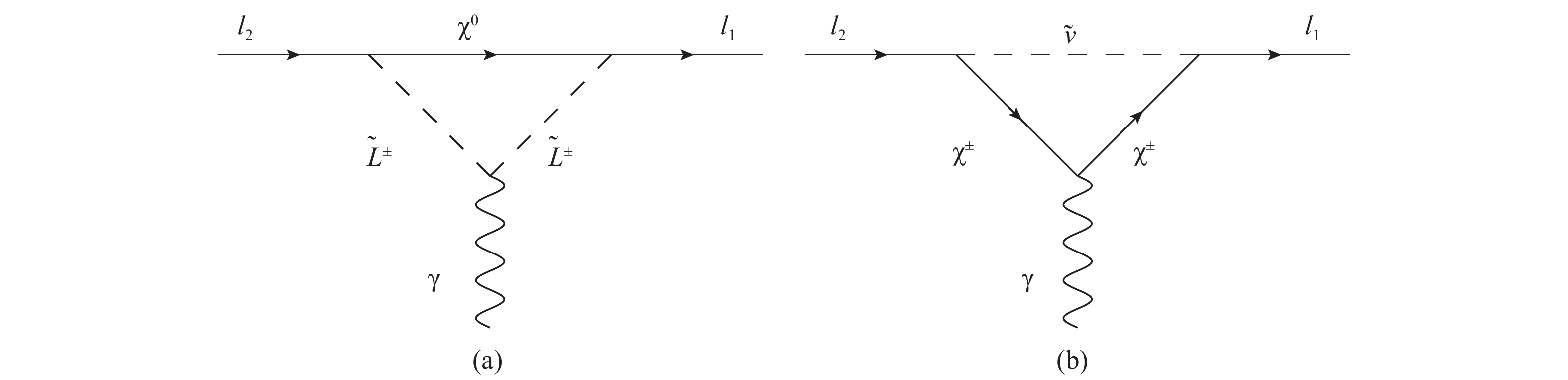
Figure 2. Feynman diagrams contributing to the LFV decays
$ l_2\rightarrow l_1\gamma $ in MRSSM.$M({l_2} \to {l_1}\gamma ) = {\epsilon ^{\mu * }}{\bar u_{{l_1}}}({p_{{l_1}}})[i{q^\nu }{\sigma _{\mu \nu }}(A + B{\gamma _5})]{u_{{l_2}}}({p_{{l_2}}}).$

(11) Then, in the limit
$ m_1\rightarrow 0 $ , the analytic expression of$ {\rm Br}(l_2\rightarrow l_1\gamma) $ is derived as${\rm Br}({l_2} \to {l_1}\gamma ) = \frac{{m_{{l_2}}^3}}{{8\pi {\Gamma _{{l_2}}}}}(|A{|^2} + |B{|^2}),$

(12) where
$ \Gamma_{l_2} $ is the total decay width of$ l_2 $ , and the form factors A and B are a combination of the form factors for every Feynman diagram in Fig. 2,$A = {A^{(a)}} + {A^{(b)}},B = {B^{(a)}} + {B^{(b)}}.$

In the limit
$ m_1\rightarrow 0 $ , the form factors$ A^{(a)} $ and$ B^{(a)} $ corresponding to Fig. 2(a) are given as$\begin{split} {A^{(a)}} =& - \displaystyle\frac{i}{{32{\pi ^2}}}[{m_2}({C_{1L}}{C_{2L}}{C_{3R}} + {C_{1R}}{C_{2R}}{C_{3L}})({{\cal C}_{12}} + {{\cal C}_{11}}) + {M_1}({C_{1L}}{C_{2R}}{C_{3L}} + {C_{1R}}{C_{2L}}{C_{3R}}){{\cal C}_2} \\&+ ({M_2}({C_{1L}}{C_{2L}}{C_{3L}} + {C_{1R}}{C_{2R}}{C_{3R}}) + {m_2}({C_{1L}}{C_{2L}}{C_{3R}} + {C_{1R}}{C_{2R}}{C_{3L}})){{\cal C}_1}],\\ {B^{(a)}} = & \displaystyle\frac{i}{{32{\pi ^2}}}[{M_1}({C_{1L}}{C_{2R}}{C_{3L}} - {C_{1R}}{C_{2L}}{C_{3R}}){{\cal C}_2} - {m_2}({C_{1R}}{C_{2R}}{C_{3L}} - {C_{1L}}{C_{2L}}{C_{3R}}) ({{\cal C}_{12}} \\& + {{\cal C}_{11}}) + ({C_{1L}}{C_{2L}}({M_2}{C_{3L}} + {m_2}{C_{3R}}) - {C_{1R}}{C_{2R}}({M_2}{C_{3R}} + {m_2}{C_{3L}})){{\cal C}_1}], \end{split}$

and the form factors
$ A^{(b)} $ and$ B^{(b)} $ corresponding to Fig. 2(b) are given as$\begin{split} &{A^{(b)}} = - \frac{{i{C_2}}}{{64{\pi ^2}}}[{M_3}({C_{1L}}{C_{3L}} + {C_{1R}}{C_{3R}})({{\cal C}_0} + 2{{\cal C}_1} + 2{{\cal C}_2}) - {m_2}({C_{1L}}{C_{3R}} + {C_{1R}}{C_{3L}}) (2{{\cal C}_{12}} + 2{{\cal C}_{11}} + {{\cal C}_1})],\\& {B^{(b)}} = \frac{{i{C_2}}}{{64{\pi ^2}}}[{M_3}({C_{1L}}{C_{3L}} - {C_{1R}}{C_{3R}})({{\cal C}_0} + 2{{\cal C}_1} + 2{{\cal C}_2}) - {m_2}({C_{1L}}{C_{3R}} - {C_{1R}}{C_{3L}}) (2{{\cal C}_{12}} + 2{{\cal C}_{11}} + {{\cal C}_1})], \end{split}$

where the loop integrals
$ \mathcal{C}_{1,2,...} $ denote$ \displaystyle\frac{i}{16\pi^2}\mathcal{C}_{1,2,...}(m_2^2,0,0;M_3,M_2,M_1) $ . The couplings corresponding to Fig. 2(a) are given as$\begin{array}{l} C_{1L}^{(a)} = iY_e^{{l_1}}U_{i2}^{1 * }Z_{k{l_1}}^V,\quad C_{1R}^{(a)} = - i{g_2}Z_{k{l_1}}^{V * }V_{i1}^1,\quad C_{2L}^{(a)} = C_{2R}^{(a)} = - ie{\delta _{ij}},\\ C_{3L}^{(a)} = - i{g_2}V_{j1}^{1 * }Z_{k{l_2}}^V,\quad C_{3R}^{(a)} = iY_e^{{l_2}}U_{j2}^1Z_{k{l_2}}^V,\quad {M_1} = {m_{\chi _i^ \pm }},\quad {M_2} = {m_{\chi _j^ \pm }},\quad {M_3} = {m_{{{\tilde \nu }_k}}}. \end{array}$

and the couplings corresponding to Fig. 2(b) are given as
$\begin{array}{l} C_{1L}^{(b)} = - i\sqrt 2 {g_1}N_{k1}^{1 * }Z_{i(3 + {l_1})}^{E * },\quad C_{1R}^{(b)} = - iY_e^{{l_1}}Z_{i(3 + {l_1})}^{E * }N_{k3}^2,\quad C_{3L}^{(b)} = - iY_e^{{l_2}}N_{k3}^{2 * }Z_{j(3 + {l_2})}^E,\\ C_2^{(b)} = ie{\delta _{ij}},\quad C_{3R}^{(b)} = - i\sqrt 2 {g_1}Z_{j(3 + {l_2})}^EN_{k1}^1,\quad {M_1} = {m_{\tilde L_i^ \pm }},\quad {M_2} = {m_{\tilde L_j^ \pm }},\quad {M_3} = {m_{\chi _k^0}}. \end{array}$

Taking
$ \delta^{13}=0 $ ,$ \delta^{23}=0 $ , we plot the theoretical prediction of Br$ (\mu\rightarrow e\gamma) $ versus$ \delta^{12} $ and Br($ Z\rightarrow e\mu $ ) versus$ \delta^{12} $ in Fig. 3(a) and Fig. 3(b), where the horizontal dotted line is the current experimental bounds of Br($ \mu\rightarrow e\gamma $ ). The solid line denotes the result calculated with parameter setup BMP1, and the dashed line denotes the result calculated with parameter setup BMP3. A linear relationship is displayed between Br$ (\mu\rightarrow e\gamma) $ or Br($ Z\rightarrow e\mu $ ) and the flavor violating parameter$ \delta^{12} $ . The prediction on Br$ (\mu\rightarrow e\gamma) $ exceeds the current experiment limit at$ \delta^{12}\sim 1.0\times 10^{-3} $ . The parameter space of$ \delta^{12} $ would have been highly suppressed below$ \mathcal{O}(10^{-3}) $ by considering the future sensitivity of the experiment, which is Br$ (\mu\rightarrow e\gamma)\sim 6 \times 10^{-14} $ [38]. The current prediction of Br($ Z\rightarrow e\mu $ ) in MRSSM is around$ \mathcal{O}(10^{-13}) $ , and this prediction is six orders of magnitude below the current limit$ \mathcal{O}(10^{-7}) $ . Based on the flavour expansion theorem, various LFV processes have been investigated in MSSM using a recently developed technique which performs a purely algebraic mass-insertion expansion of the amplitudes [39]. Considering the constraints from radiative charged lepton decays, upper bounds on the flavor violating parameters$ \delta^{12}_l $ ($ \Delta^{21}_{LL} $ ) and$ \delta^{12}_r $ ($ \Delta^{21}_{RR} $ ) are given in Ref. [39] with$ \delta^{12}_l \sim 8.4\times 10^{-4} $ ($ \tan \beta $ = 2) and$\delta^{12}_r \sim $ $ 5.0\times 10^{-3} $ ($ \tan \beta $ = 2). It shows that flavor violating$ \mu $ lepton decays still provide the most stringent bounds on supersymmetric effects.
Figure 3. (a) Br(
$ \mu\rightarrow e\gamma $ ) versus$ \delta^{12} $ ; (b) Br($ Z\rightarrow e\mu $ ) versus$ \delta^{12} $ ; (c) Br($ \tau\rightarrow e\gamma $ ) versus$ \delta^{13} $ ; (d) Br($ Z\rightarrow e\tau $ ) versus$ \delta^{13} $ ; (e) Br($ \tau\rightarrow \mu\gamma $ ) versus$ \delta^{23} $ ; (f) Br($ Z\rightarrow \mu\tau $ ) versus$ \delta^{23} $ . The horizontal dotted line in the left panel denotes the current experimental bounds. The solid line denotes the result with BMP1, and the dashed line denotes the result with BMP3.Taking
$ \delta^{12}=0 $ ,$ \delta^{23}=0 $ , we plot the theoretical prediction of Br$ (\tau\rightarrow e\gamma) $ versus$ \delta^{13} $ and Br($ Z\rightarrow e\tau $ ) versus$ \delta^{13} $ in Fig. 3(d) and Fig. 3(d), where the horizontal dotted line is the current experimental bounds of Br($ \tau\rightarrow e\gamma $ ). The solid line denotes the result calculated with parameter setup BMP1, and the dashed line denotes the result calculated with parameter setup BMP3. Both predictions on Br$ (\tau\rightarrow e\gamma) $ and Br($ Z\rightarrow e\tau $ ) decrease as the flavor violating parameter$ \delta^{13} $ varies from 0.9 to 0.1. The prediction on Br$ (\tau\rightarrow e\gamma) $ exceeds the current experiment limit at$ \delta^{13}\sim 0.75 $ . Considering the future experimental expectation on Br$ (\tau\rightarrow e\gamma) $ , which is approximately$ 2.3\times 10^{-9} $ [40], the parameter space of$ \delta^{13} $ would have been suppressed below$ 0.3 $ . The upper theoretical prediction on Br($ Z\rightarrow e\tau $ ) in MRSSM is around$ \mathcal{O}(10^{-8}) $ , and this prediction is two orders of magnitude below the current limit$ \mathcal{O}(10^{-6}) $ . Recent upper bounds on the flavor violating parameters$ \delta^{13}_l $ ($ \Delta^{31}_{LL} $ ) and$ \delta^{13}_r $ ($ \Delta^{31}_{RR} $ ) in MSSM are given by$ \delta^{13}_l \sim 4.6\times 10^{-1} $ ($ \tan \beta $ =2) and$ \delta^{13}_r \sim \mathcal{O}(1) $ ($ \tan \beta $ =2) [39].Taking
$ \delta^{12}=0 $ ,$ \delta^{13}=0 $ , we plot the theoretical prediction of Br$ (\tau\rightarrow \mu\gamma) $ versus$ \delta^{23} $ and Br($ Z\rightarrow \mu\tau $ ) versus$ \delta^{23} $ in Fig. 3(e) and Fig. 3(f), where the horizontal dotted line is the current experimental bounds of Br($ \tau\rightarrow \mu\gamma $ ). The solid line denotes the result calculated with parameter setup BMP1, and the dashed line denotes the result calculated with parameter setup BMP3. Both predictions on Br$ (\tau\rightarrow \mu\gamma) $ and Br($ Z\rightarrow \mu\tau $ ) decrease sharply as the flavor violating parameter$ \delta^{13} $ is close to 0.1. The prediction on Br$ (\tau\rightarrow \mu\gamma) $ exceeds the current experiment limit at$ \delta^{23}\sim 0.8 $ . Considerng the future experimental expectation on Br$ (\tau\rightarrow \mu\gamma) $ , which is approximately ($ 1.8\times 10^{-9} $ ) [40], the parameter space of$ \delta^{23} $ would have also been suppressed below$ 0.3 $ . The upper theoretical prediction on Br($ Z\rightarrow \mu\tau $ ) in MRSSM is also around$ \mathcal{O}(10^{-8}) $ , and this prediction is three orders of magnitude below the current limit$ \mathcal{O}(10^{-5}) $ . Recent upper bounds on the flavor violating parameters$ \delta^{23}_l $ ($ \Delta^{32}_{LL} $ ) and$ \delta^{23}_r $ ($ \Delta^{32}_{RR} $ ) in MSSM are given by$ \delta^{23}_l \sim 5.3\times 10^{-1} $ ($ \tan \beta $ =2) and$ \delta^{23}_r \sim \mathcal{O}(1) $ ($ \tan \beta $ =2) [39].Recently, the ATLAS collaboration has released a search for chargino-neutralino production in two and three lepton final states, employing RJR techniques that target specific event topologies [25], which state that charginos and neutralinos must be heavier than 600 GeV at 95% CL. To be compatible with the experimental limit, the parameters
$ M_D^W $ ,$ M_D^B $ ,$ \mu_u $ , and$ \mu_d $ , which dominant the masses of charginos and neutralinos, should be enlarged. The selection of BMP1 and BMP3 is shown in Fig.8.2 in Ref. [41], where the parameters are set to BMP1 and BMP3 for the top and bottom row, respectively, and the benchmark point is marked by a star in each plot. It is shown that the valid region is$ \mu_u(\mu_d)< $ 500 GeV for BMP1, and this leads to at least two sparticle mass lighter than 600 GeV. For BMP3, the valid region for$ \mu_u(\mu_d) $ can be enlarged above 600 GeV along with$ M_D^W $ and$ M_D^B $ . Then, to quantitatively study the LFV decays of Z boson, we perform a scan under BMP3 over the parameters$ M_D^W $ and$ M_D^B $ , with$ \mu_u(\mu_d)= $ 600 GeV. The ranges of the variation over the MRSSM parameters are displayed in Table 6; all mass parameters are in GeV. Moreover, the three flavor violating parameters$ \delta^{12} $ = 10-3,$ \delta^{13} $ =0.3, and$ \delta^{23} $ =0.3 are assumed.parameter Min Max step $M_D^W$ 

600 800 10 $M_D^B$ 

600 1000 10 Table 6. Range of input parameters for the numerical scan with BMP3.
Over a general scan of thousands of points in parameter spaces according to Table 6, we display the predictions on Br(
$ Z\rightarrow e\mu $ ), Br($ Z\rightarrow e\tau $ ), and Br($ Z\rightarrow \mu\tau $ ) as a function of$ M_D^W $ in Fig. 4(a), (b), and (c), respectively. It shows that the predictions on Br($ Z\rightarrow e\mu $ ), Br($ Z\rightarrow e\tau $ ), and Br($ Z\rightarrow \mu\tau $ ) decrease as$ M_D^W $ varies from 600 GeV to 800 GeV. For Br($ Z\rightarrow e\mu $ ), the range of the prediction is narrowed above$ \mathcal{O}(10^{-14}) $ at$ M_D^W $ =600 GeV, and narrowed to$ \mathcal{O}(10^{-15}-10^{-14}) $ at$ M_D^W $ =800 GeV. For Br($ Z\rightarrow e\tau $ ) and Br($ Z\rightarrow \mu\tau $ ), the range of the prediction is narrowed above$ \mathcal{O}(10^{-9}) $ at$ M_D^W $ =600 GeV and$ \mathcal{O}(10^{-10}-10^{-9}) $ at$ M_D^W $ =800 GeV.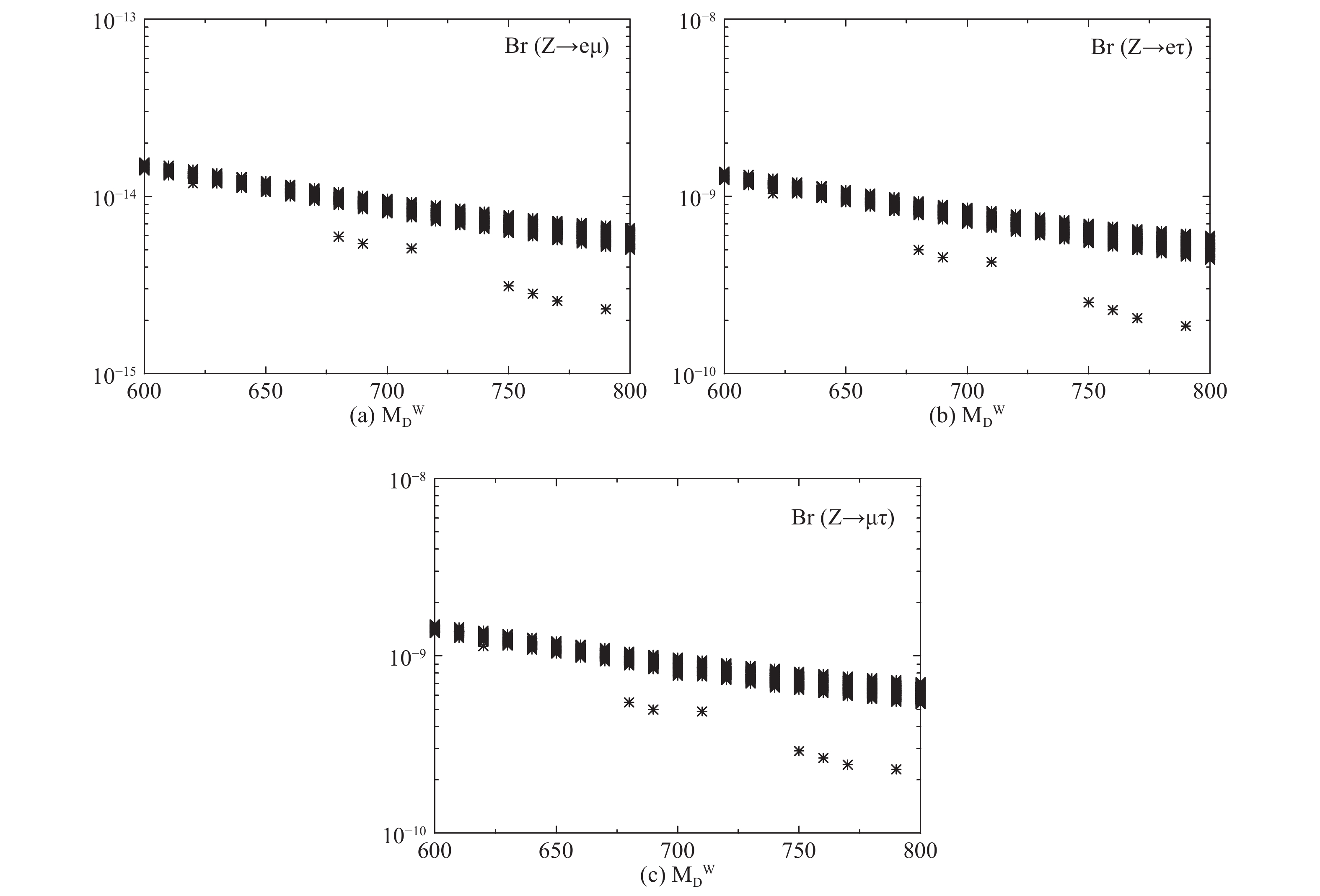
Figure 4. (a) Br(
$ Z\rightarrow e\mu $ ) versus$ M_D^W $ ; (b) Br($ Z\rightarrow e\tau $ ) versus$ M_D^W $ ; (c) Br($ Z\rightarrow \mu\tau $ ) versus$ M_D^W $ . All points satisfy the experimental bound in Table 5. -
In this work, considering the constraints on the parameter space from radiative charged lepton decays Br(
$ l_2\rightarrow l_1\gamma $ ), we analyzed the LFV decays of$ Z\rightarrow l_1 l_2 $ as a function of the flavor violating off-diagonal entries$ \delta^{12} $ ,$ \delta^{13} $ and ,$ \delta^{23} $ in the framework of the MRSSM. A summary on the upper limits on flavor violating parameters in MRSSM is provided in Table 7, where the results in MSSM are also included for reference. It shows that the upper limits for two different models are very close to each other.parameters MRSSM MSSM( $ \Delta^{IJ}_{LL} $ /

$ \Delta^{IJ}_{RR} $ [39])

$ \delta^{12} $ 

$ 1.0\times 10^{-3} $ 

$ 8.4\times 10^{-4} $ /

$ 5.0\times 10^{-3} $ 

$ \delta^{13} $ 

$ 3.0\times 10^{-1} $ 

$ 5.3\times 10^{-1} $ /

$ \mathcal{O}(1) $ 

$ \delta^{23} $ 

$ 3.0\times 10^{-1} $ 

$ 4.6\times 10^{-1} $ /

$ \mathcal{O}(1) $ 

Table 7. Upper limits on off-diagonal entries
$ \delta^{12} $ ,$ \delta^{13} $ and$ \delta^{23} $ .Table 8. Upper predictions on LFV decays of Z boson in MRSSM.
The LFV decays of
$ Z\rightarrow l_i l_j $ depend strongly on the three flavor violating parameters$ \delta^{ij} $ in soft breaking terms$ m_l $ and$ m_r $ , i.e., if set$ \delta_{ij} $ = 0, then the branching ratios of$ Z\rightarrow l_i l_j $ equal zero. Considering the constraints from$ l_2\rightarrow l_1\gamma $ , we summarize the theoretical predictions of$ Z\rightarrow l_1 l_2 $ in MRSSM in Table 8, and the value is taken from Fig. 4 with$ M_D^W $ =600 GeV. The upper prediction on Br($ Z\rightarrow e\mu $ ) is seven orders of magnitude below current experimental bound, and we may make further efforts to observe it in a future experiment. The upper prediction on Br($ Z\rightarrow e\tau $ ) and Br($ Z\rightarrow \mu\tau $ ) are at the same order and close to the current experimental bound. Thus, the observations of LFV decays$ Z\rightarrow e\tau $ and$ Z\rightarrow \mu\tau $ may be more promising in a future experiment.
LFV decays of Z boson in Minimal R-symmetric Supersymmetric Standard Model
- Received Date: 2018-09-02
- Accepted Date: 2019-01-09
- Available Online: 2019-04-01
Abstract: A future Z-factory will offer the possibility of studying rare Z decays


 DownLoad: