


 Abstract
 HTML
HTML Reference
 Related
 PDF
PDF


-
The nucleon-nucleon (NN) interaction is an essential physical phenomenon for interpreting the world of nuclear physics, which determines how protons and neutrons are composed in a complex quantum system. It is regarded as a residual of the strong interaction in the low energy regime, where the quantum chromodynamics (QCD) theory cannot be solved perturbatively. Therefore, the NN interaction is usually described by the meson exchange model first proposed by Yukawa [1]. In 1960s, heavier bosons were included in this scheme to deal with the intermediate- and short-range NN interactions. Generally speaking, there are two kinds of nuclear interactions. The first kind is based on the free NN scattering data, such as the differential cross-sections and polarization, and is called the realistic NN interaction, while the other is based on the properties of finite nuclei and infinite nuclear matter [2-7]. The latter is called the effective NN interaction in terms of nuclear medium effects.
A reasonable model of the NN force should not only describe the interaction behavior of nucleons, i.e., the strong repulsion at short range, the large attraction at intermediate range, and the small tail at long range, but also satisfy several basic symmetries, such as the rotational invariance in space, translational invariance and space reflection invariance. Therefore, the NN forces were initially constructed in the coordinate space in terms of the angular momentum operators, which fulfill the symmetry requirements, such as the Hamada-Johnston potential [8] and Reid68 potential [9] in the non-relativistic framework. On the other hand, the one-boson-exchange (OBE) potentials were based on the development of quantum field theory, where the nucleons interact with each other by exchanging several mesons whose masses are below 1 GeV [10]. With important achievements of the OBE potentials, more degrees of freedom, like the multi-meson exchange and
$ \Delta $ isobar, were introduced, which led to the full Bonn models [11, 12].In 1990s, the effects of charge independence breaking (CIB) and charge symmetry breaking (CSB) were introduced in the nuclear force based on detailed analyses of thousands of NN scattering data. High precision NN forces were constructed, such as the Reid93, Nijmegen 93, Nijmegen I, Nijmegen II, and AV18 potentials [13, 14]. The chiral perturbation theory was also applied for deriving the NN interaction, first proposed by Weinberg [15-17], and chiral NN potentials have been built up to the fifth-order expansion [18-28]. In 2000, a covariant charge-dependent OBE (CD-Bonn) potential was proposed by Machleidt as a very high precision NN interaction, which describes the NN scattering data very well, with
$ \chi^2/{\rm datum}\sim 1 $ [29]. The$ \omega,\; \rho, \; \pi $ mesons and two scalar mesons$ \sigma_1 $ and$ \sigma_2 $ were included in the CD-Bonn potential, which is widely applied to study the properties of nuclear systems, from light nuclei to heavy nuclei and infinite nuclear matter.The pion, the first meson discovered, largely determines the behavior of the NN interaction in the long-range region. As a Goldstone boson, it also describes one of the crucial features of the QCD theory, its chiral symmetry. However, the coupling between the pion and a nucleon has two possible sources, namely the pseudoscalar (PS) and pseudovector (PV) coupling. In fact, the on-shell amplitudes of one-pion exchange with PS and PV
$ \pi NN $ couplings are identical. Caia et al. also examined the differences between the PS and PV couplings of the pion and$ \eta $ meson in the NN potentials in terms of two kinds of scattering equations, i.e. Lippmann-Schwinger and Thompson equations [30]. It was found that the differences of phase shifts and binding properties between the PS and PV couplings in a two-nucleon system are very small in these two approaches. The largest difference appears in the mixing parameter$ \varepsilon_1 $ in the$ J = 1 $ channel, which is strongly related to the strength of the tensor component of the NN interaction. Therefore, the D-state probability, quadrupole moment and asymptotic S-state amplitude of the deuteron show few differences between the PS and PV couplings.On the other hand, in the calculations of pion-nucleon scattering, the unitarity and analytic continuation of
$ \pi N $ to$ \pi\pi\rightleftharpoons N\bar N $ etc., the PV coupling was preferred [31, 32]. In the chiral perturbation theory, the coupling between the pion and a nucleon was also taken as of the PV type in the low energy region to analyze the pion electroproduction and photoproduction [33, 34]. Furthermore, when the NN potentials with PS coupling were used in the relativistic nuclear many-body problems, a spurious strong attraction was generated due to the strong coupling to negative energy states, which is absent in the non-relativistic framework. The PV coupling suppresses the coupling to antinucleons, since its matrix element between the nucleon and antinucleon vanishes for the on-shell scattering [35]. As a result, PV couplings were adopted in the Bonn A, B, and C potentials, which were successfully used with the relativistic Bruckner-Hartree-Fock method, and led to relatively reasonable saturation properties of nuclear matter [36].In this work, we develop a revised version of the CD-Bonn potential with PV coupling for pions, which can be applied in the relativistic nuclear many-body problems. The theoretical framework of the CD-Bonn potential is kept, but we use the PV coupling instead of the PS coupling between pions and nucleons. At the present stage, the coupling constants and the cut-off momenta for the form factors for various mesons are determined by fitting the phase shifts from Nijmegen PWA. The paper is arranged as follows: in Sec. 2, the necessary formulas for the OBE potential and NN scattering are presented. In Sec. 3, the CD-Bonn potentials with PV coupling are shown, and the properties of the two-nucleon scattering and binding states using these potentials are presented. A summary and outlook are given in Sec. 4.
-
In the conventional OBE potential, there are six mesons whose masses are below 1 GeV, i.e. the
$ \sigma,\; \omega,\; \rho,\; \pi,\; \eta,\; \delta $ mesons [11, 12]. In the CD-Bonn potential, two heavier mesons,$ \delta $ and$ \eta $ were not considered [29]. Furthermore, to better simulate the broad contribution from the$ 2\pi+\pi\rho $ exchange between two nucleons in the intermediate range, two scalar mesons$ \sigma_1 $ and$ \sigma_2 $ were included. The Lagrangians which describe the meson-nucleon couplings in the CD-Bonn potential are given as:$ {\cal L}_{\sigma NN} = -g_\sigma \bar{\psi}\psi\varphi^{(\sigma)}, $

(1) $ {\cal L}_{\omega NN} = -g_\omega \bar{\psi}\gamma^\mu \psi \varphi^{(\omega)}_\mu, $

(2) $\begin{split} {{\cal L}_{\rho NN}} =& - {g_\rho }\bar \psi {\gamma ^\mu }\vec \tau \psi \cdot \vec \varphi _\mu ^{(\rho )}\\ &- \frac{{{f_\rho }}}{{4{M_p}}}\bar \psi {\sigma ^{\mu \nu }}\vec \tau \psi \cdot [{\partial _\mu }\vec \varphi _\nu ^{(\rho )} - {\partial _\nu }\vec \varphi _\mu ^{(\rho )}], \end{split}$

(3) for the
$ \sigma,\; \omega $ , and$ \rho $ mesons. Here,$ \psi $ denotes the nucleon field and$ \varphi $ represents the meson field. The tensor coupling between the$ \omega $ meson and nucleon is neglected due to its small strength. To apply the CD-Bonn potential to a study of the nuclear many-body system in the relativistic framework, the pseudovector (PV) coupling between the pion and nucleon is taken in this work,$ {\cal L}_{\pi NN}^{({\rm pv})} = -\frac{f_\pi}{m_{\pi}}\bar{\psi}\gamma^5\gamma^\mu\vec{\tau}\psi\cdot\partial_\mu\vec{\varphi}^{(\pi)}, $

(4) where the coupling constant
$ f_\pi $ is related to the pseudoscalar (PS) coupling constant$ g_\pi $ , by the on-shell-equivalent relation [36]$ \frac{g_\pi}{M_1+M_2} = \frac{f_\pi}{m_\pi}. $

(5) Here,
$ M_1 $ and$ M_2 $ are the masses of the two nucleons, and$ m_\pi $ is the pion mass.The contribution of each meson
$ \alpha $ to the NN interaction is expressed analytically by the scattering amplitude from the quantum field theory [12],$ i\bar{V}_\alpha({ q}',{ q}) = \bar{u}_1({ q}')\Gamma_1^{\alpha}u_1({ q})\frac{P_\alpha}{{ k}^2 +m_\alpha^2} \bar{u}_2(-{ q}')\Gamma_2^{\alpha}u_2(-{ q}), $

(6) where
$ { q}' $ and$ { q} $ are the relative momenta of the two nucleons in the in- and out-scattering states in the center-of-mass (CM) framework, and$ { k} = { q}'-{ q} $ . The vertex$ \Gamma_{i}^\alpha\; (i = 1,2) $ and the meson propagator$ P_\alpha/({ k}^2+m_\alpha^2) $ can be directly generated from the Lagrangians in Eqs. (1) and (4).$ u({ q}) $ is the Dirac spinor of the nucleon. The static approximation is adopted in the denominator of the meson propagator to obtain an energy independent NN potential. The explicit expressions for the mesons involved are shown in the Appendix.In addition, a form factor
$ {\cal F}_\alpha({ k}^2) $ is introduced to treat the finite size of the nucleon. There are many choices for$ {\cal F}_\alpha({ k}^2) $ , like the monopole form, dipole form, exponential form, etc. In the CD-Bonn potential, the monopole form factor is adopted at each vertex between the meson and nucleon,$ {\cal F}_\alpha({ k}^2) = \frac{\Lambda_\alpha^2-m_\alpha^2}{\Lambda_\alpha^2+{ k}^2}, $

(7) where
$ m_\alpha $ is the mass of the meson and$ \Lambda_\alpha $ the corresponding cut-off momentum.The Bethe-Salpeter (BS) equation is used to describe the NN scattering in the relativistic framework. However, it is very difficult to solve this four-dimensional integral equation. A three-dimensional reduction is necessary to get numerical results. There are many schemes to do such a reduction, such as the Blankenbecler-Sugar (BbS) choice [37], Thompson choice [38], Kadyshevsky choice [39] etc. The BbS choice was taken in the original CD-Bonn potential. The Bonn A, B, C potentials adopted the Thompson choice. It must be emphasized that our goal is to obtain a revised CD-Bonn potential with PV coupling and to compare it with the old version. Therefore, the BbS choice is used in this work.
When the BbS choice is taken in the propagator part, the BS equation in the two-nucleon CM frame is reduced to [29],
$ \bar {T}({ q}',{ q}) = \bar V({ q}',{ q})+ \int \frac{{\rm d}^3 { k}}{(2\pi)^3} \; \bar{V}({ q}',{ k})\frac{M^2}{E_{ k}}\frac{1}{{ q}^2-{ k}^2+{\rm i}\epsilon}\bar T({ k},{ q}), $

(8) After taking minimal relativity and the form factors, the complete interaction is constructed as
$V({{{q}}^\prime },{{q}}) = \sum\limits_{{\rm{All}}\;{\rm{Mesons}}} {\mathcal{F}_\alpha ^2} ({{{k}}^2})\sqrt {\frac{M}{{E'}}} {\bar V_\alpha }({{{q}}^\prime },{{q}})\sqrt {\frac{M}{E}}, $

(9) where
$ E = \sqrt{{ q}^2 +M^2} $ ,$ E_{ k} = \sqrt{{ k}^2 +M^2} $ and$ E' = \sqrt{{ q}'^2 +M^2} $ are the initial, intermediate and final energies, respectively. The scattering equation for the two-nucleon system is then given as a three-dimensional BbS equation$ T({ q}',{ q}) = V({ q}',{ q})+\int\frac{{\rm d}^3 { k}}{(2\pi)^3} \; V({ q}',{ k})\frac{M}{{ q}^2-{ k}^2+{\rm i}\epsilon}T({ k},{ q}). $

(10) This equation has a similar form as the Lippmann-Schwinger equation. The phase shifts for NN scattering can be obtained from the on-shell T-matrix. The mathematical details are presented in the Appendix.
-
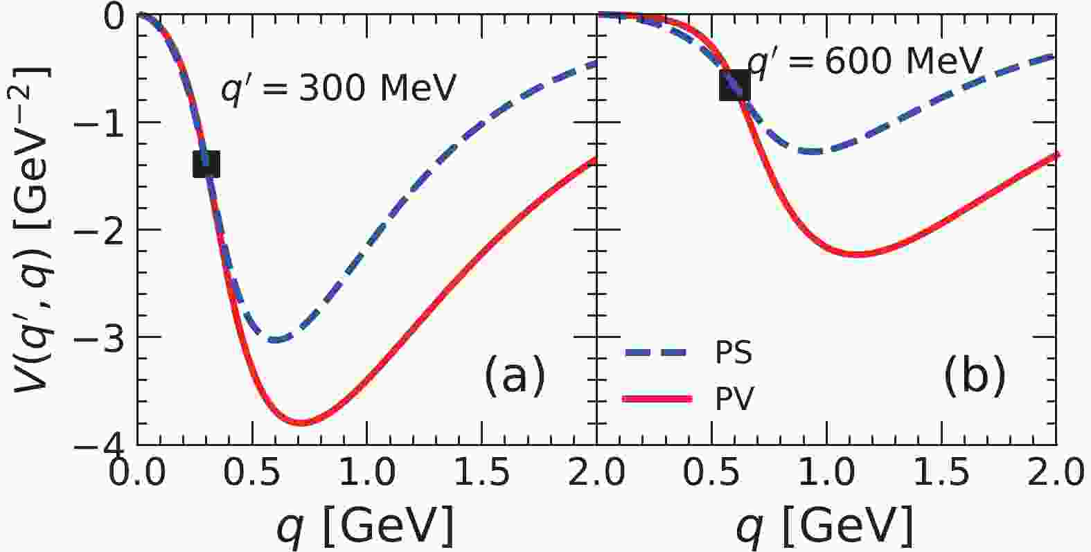
The on-shell matrix elements for the one-pion-exchange (OPE) potentials with the PS and PV couplings are identical, while their off-shell behavior is completely different, especially in the high momentum region. The half-on-shell matrix elements for the OPE potential
$ V(q,q') $ with PS and PV couplings in the$ ^3S_1 $ -$ ^3D_1 $ channel and fixed on-shell momenta$ q' = 300 $ MeV and$ q' = 600 $ MeV, are shown in Fig. 1 (a) and Fig. 1 (b). The cut-off momentum$ \Lambda_\pi = 1720 $ MeV and the pion-nucleon coupling constant$ g_\pi^2/4\pi = 13.6 $ are used. The matrix elements for the OPE potential in the$ ^3S_1 $ -$ ^3D_1 $ channel are generated by its tensor component. It is found that in the higher momentum region the PV coupling gives a higher attractive contribution than the PS coupling, while they have similar strength for on-shell momenta.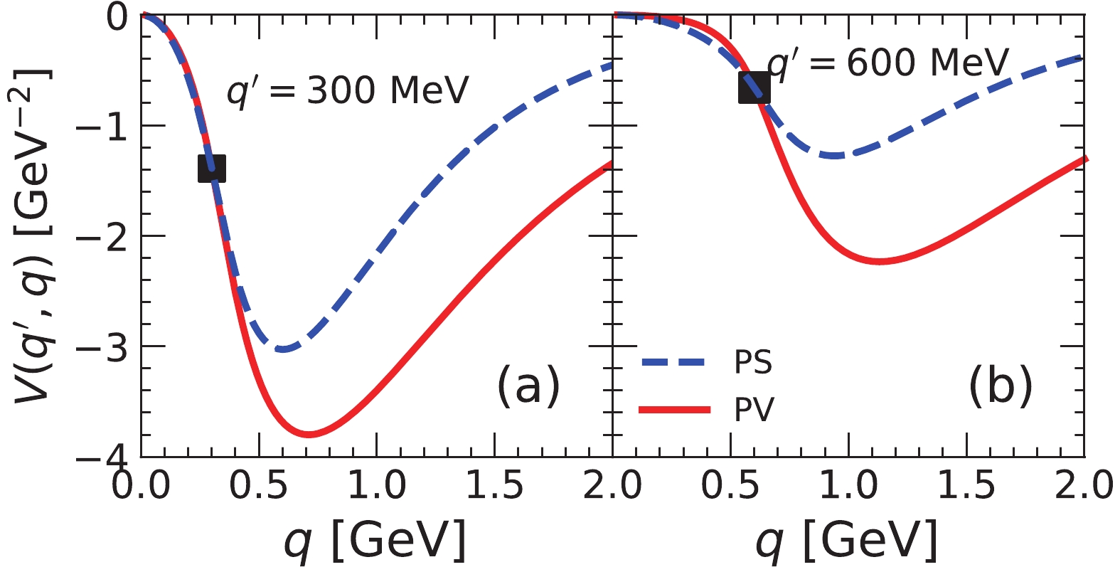
Figure 1. (color online) The half-on-shell matrix elements for the OPE potential in the
$^3S_1$ -$^3D_1$ coupled channel. In panel (a), the on-shell point is at$q' = 300$ MeV, and in panel (b) it is at$q' = 600$ MeV. The dashed line represents the PS coupling, while the solid curve denotes the PV coupling.The PV coupling constant
$ f_\pi $ is related to the PS coupling constant$ g_\pi $ , as shown in Eq. (5). Traditionally, the$ \pi N $ coupling constants are expressed as$ g_\pi $ for both the PS coupling and PV coupling. To consider the charge symmetry breaking effect,$ g_\pi $ for the neutron-neutron (nn), proton-proton (pp), and neutron-proton (np) systems should be distinguished. Its value for the np and nn systems can be expressed by$ g_\pi(pp) $ with the following relations [29],$\begin{split} \frac{{g_\pi ^2(np)}}{{4\pi }} = &{\left( {\frac{{{M_p} + {M_n}}}{{2{M_p}}}} \right)^2}\frac{{g_\pi ^2(pp)}}{{4\pi }},\\ \frac{{g_\pi ^2(nn)}}{{4\pi }} = &{\left( {\frac{{{M_n}}}{{{M_p}}}} \right)^2}\frac{{g_\pi ^2(pp)}}{{4\pi }}. \end{split}$

(11) In this work, the coupling constants and the cut-off momenta of the
$ \omega $ and$ \rho $ mesons are directly taken from the original CD-Bonn potential with PS coupling in all channels. The effect of the tensor force in a nuclear many-body system is a very hot topic in recent research. The strength of the OPE potential determines directly the magnitude of the tensor force in the NN interaction. Therefore, we choose three pion-nucleon coupling constants to produce different tensor components, following the idea of the Bonn A, B, C potentials [36]. The corresponding coupling constants and cut-off momenta are listed in Table 1. To reduce the uncertainties of the coupling constants as much as possible, there is a constraint between$ g_\pi $ and$ \Lambda_\pi $ in free space,$ {\cal F}^2_\pi({ k}^2 = 0)\cdot g_\pi^2/4\pi = 13.42 $ . For convenience, these three potentials with PV coupling are called the pvCD-Bonn A, B, C potentials in the following discussion.$m_a$ /MeV

A B C $g_a^2/4\pi$ 

$f_a/g_a$ 

$\Lambda_a$ /GeV

$g_a^2/4\pi$ 

$f_a/g_a$ 

$ \Lambda_a$ /GeV

$g_a^2/4\pi$ 

$f_a/g_a$ 

$ \Lambda_a$ /GeV

$\pi^0$ (139.57)

13.9 1.12 13.7 1.50 13.6 1.72 $\pi^\pm$ (134.98)

13.9 1.12 13.7 1.50 13.6 1.72 $\rho^{0},\rho^\pm$ (770)

0.84 6.1 1.31 0.84 6.1 1.31 0.84 6.1 1.31 $\omega$ (782)

20 1.50 20 1.50 20 1.50 Table 1. The coupling constants and cut-off momenta for the pion and
$\omega,\; \rho$ mesons for the pvCD-Bonn A, B, C potentials.The form factor can considerably suppress the OPE potential in the high momentum region. In Fig. 2 (a), the product of
$ g^2_\pi/4\pi $ and$ {\cal F}^2_\pi(k^2) $ , which can be regarded as the effective coupling constant, for the pvCD-Bonn A, B, C potentials is given as a function of momentum. Due to the influence of the form factors, the effective coupling constants decrease rapidly with momentum. The$ \pi N $ coupling constant for pvCD-Bonn A is the largest. However, its pion contribution is the smallest of the three pvCD-Bonn potentials due to its minimum cut-off momentum. Its magnitude at$ k = 1000 $ MeV is nearly half of that for the pvCD-Bonn C potential.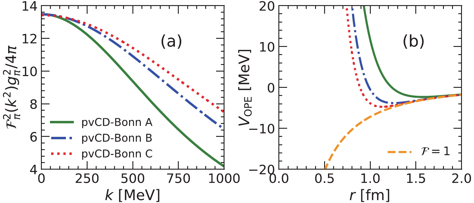
Figure 2. (color online) The effective
$\pi NN$ coupling strengths of the pvCD-Bonn A, B, C potentials as function of the transferred momentum (a), and the corresponding isospin-singlet and spin-triplet OPE potentials in coordinate space (b).In Fig. 2 (b), the local OPE potentials for pvCD-Bonn A, B, C in the isospin-singlet and spin-triplet channels, i. e.
$ T = 0,\; S = 1 $ , are plotted in coordinate space. To show the influence of the form factor, the free OPE potential is also shown for comparison. The form factor mainly plays a role in the high momentum region. Correspondingly, it exhibits the cut-off effect at short range in coordinate space. When the relative distance between two nucleons is larger than$ 1.5 $ fm, the OPE potentials with and without the form factor are almost identical. In the short-range region, the form factor changes the OPE potentials significantly. -
To describe the CSB of the NN interaction precisely, the coupling constants and cut-off momenta of the
$ \sigma_1 $ and$ \sigma_2 $ mesons are fitted to reproduce the phase shifts for NN scattering analyzed by the Nijmegen group in 1993, i.e. Nijmegen PWA [13], for each partial wave with$ J\leq 4 $ following the scheme of Machleidt [29]. The NN laboratory energy is up to$ 300 $ MeV. The BbS equation is solved by the matrix inversion method [40] by discretizing the Gauss-Laguerre quadrature. Free parameters are searched for by the numerical minimization Fortran program MINUIT.The fitting function is defined as
${\chi ^2} = \frac{1}{N}\mathop \sum \limits^N {\left( {\frac{{{\delta _{{\rm{OBE}}}} - {\delta _{{\rm{NM}}}}}}{{{\delta _{{\rm{NM}}}}}}} \right)^2}, $

(12) where
$ \delta_{\rm OBE} $ is the phase shift predicted by the pvCD-Bonn A, B, C potentials, and$ \delta_{\rm NM} $ are the data from Nijmegen PWA. Consequently,$ \chi^2 $ used in this work only reflects the deviation of phase shifts between the theoretical calculations and Nijmegen PWA. The fitting energies cover the NN laboratory energy range$ 0-350 $ MeV. We take$ E_{\rm lab} = 1,\; 5,\; 10,\; 25,\; 50,\; 100,\; 150,\; 200,\; 250,\; 300,\; $ $350 $ MeV in each channel. The Nijmegen PWA data are obtained from http://nn-online.org.As shown in the original CD-Bonn potential, in the isospin
$ T = 1 $ channel, the$ pp, nn $ and np interactions are not independent due to CSB and CIB. If one of these three interactions is determined, the other two channels are fixed. Therefore, we first fit the pp interaction, whose scattering data have been measured most accurately. The Coulomb interaction is included in the pp scattering as a long-range potential. The asymptotic wave functions are related to the regular and irregular Coulomb functions. The details are shown in the Appendix of Ref. [29].With different strengths of OPE potentials, the pvCD-Bonn A, B, C interactions are obtained. The phase shifts for each partial wave with the total angular momentum
$ J\leqslant 3 $ and the mixing parameter$ \varepsilon_2 $ are shown in Fig. 3. The fitted data from Nijmegen PWA are shown as solid triangles, the phase shifts for the CD-Bonn potential with PS coupling are presented as open circles, and those for the latest chiral N4LO potential with$ \Lambda = 500 $ MeV by Entem et al., [27] are given as crosses. It is found that all data from Nijmegen PWA can be described very well and are consistent among the three potentials. There are slight differences among the pvCD-Bonn A, B, C potentials for the phase shifts in the$ ^3F_2 $ channel and the mixing parameter$ \varepsilon_2 $ at high$ E_{\rm lab} $ . The$ ^3F_2 $ and$ ^3P_2 $ channels couple due to the tensor operator. The mixing parameter$ \varepsilon_2 $ represents the strength of the NN tensor interaction for$ J = 2 $ . Therefore, these differences are easily understood as due to different tensor components in the pvCD-Bonn A, B, C interactions. The phase shifts and mixing parameters generated by the pvCD-Bonn C interaction are consistent with those from Nijmegen PWA and the CD-Bonn potential for each partial wave, where the amplitudes of the OPE potential are largest. Actually, similar results were obtained for the Bonn A, B, C potentials. Furthermore, it can be seen that the phase shifts in the$ ^3F_2 $ channel for the chiral potential clearly deviate from the others. This is because the phase shifts in the$ ^3F_2 $ channel should be correctly described only by the sixth-order expansion of the chiral potential [28].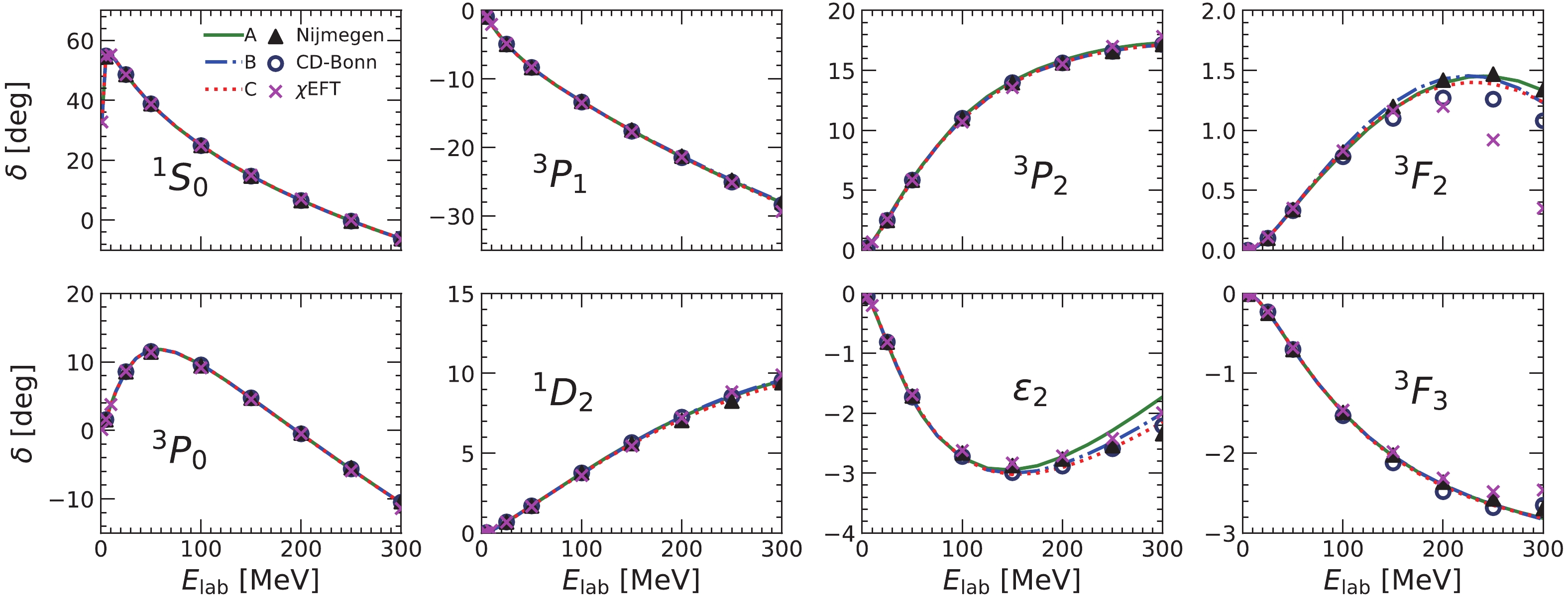
Figure 3. (color online) The pp phase shifts and mixing parameters as function of laboratory energy,
$E_{\rm lab}$ ($J\leqslant 3$ ). The triangles, open circles, and crosses represent the phase shifts from Nijmegen PWA, the CD-Bonn potential and the chiral N4LO potential by Entem et al., respectively.The nn interactions were generated based on the pp interactions by interchanging the proton mass with the neutron mass, and fitting the coupling constants of the
$ \sigma_1 $ and$ \sigma_2 $ mesons to the CSB phase shift differences arising from the nucleon mass splitting, OBE and the two-boson exchange given by Machleidt in Ref. [29]. The phase shifts and mixing parameters for the nn interactions for the pvCD-Bonn A, B, C potentials are shown in Fig. 4. There are no phase shift data for nn scattering in Nijmegen PWA. Therefore, the phase shifts and mixing parameters for the pvCD-Bonn A, B, C potentials are only compared with the results for the CD-Bonn potential with PS coupling and the latest N4LO chiral potential. They are slightly different for the coupled channels, the$ ^3F_2 $ -$ ^3P_2 $ waves and mixing parameter$ \varepsilon_2 $ , but are very similar to the pp case.
Figure 4. (color online) The nn phase shifts and mixing parameters for the pvCD-Bonn A, B, C potentials and partial waves (
$J\leqslant 3$ ). The open circles and crosses denote the results for the CD-Bonn potential and the chiral N4LO potential by Entem et al., respectively.For the
$ np\; (T = 1) $ potentials, an analogous procedure was followed. The proton mass was replaced by the average mass,$ \widetilde M = \sqrt{M_n M_p} $ . Furthermore, in the OPE potential, the positive and negative pions were also included in the exchange between the two nucleons, whose masses are slightly different from the$ \pi^0 $ mass. The coupling constants of$ \sigma_1 $ and$ \sigma_2 $ for the np potentials were determined by adjusting the CIB phase shift differences arising from the pp and np potentials, nucleon mass splitting, OPE, two-boson exchange, irreducible$ \pi\gamma $ exchange, and the Coulomb force. The phase shifts and mixing parameters for$ np \; (T = 1) $ and each partial wave for$ J\leqslant 3 $ are presented as function of laboratory kinetic energy in Fig. 5. The differences between the phase shifts and mixing parameters for the pvCD-Bonn A, B, C potentials in the$ ^3F_2 $ channel and$ \varepsilon_2 $ still exist.
Figure 5. (color online) The
$np\; (T = 1)$ phase shifts and mixing parameters for different partial waves ($J\leqslant 3$ ). The triangles, open circles, and crosses represent the phase shifts from Nijmegen PWA, the CD-Bonn potential, and the chiral N4LO potential by Entem et al., respectively.For the np potential, there is another possibility in the
$ T = 0 $ channel. The corresponding coupling constants of the$ \sigma_1 $ and$ \sigma_2 $ mesons are directly adjusted to reproduce the phase shifts from Nijmegen PWA. The phase shifts and mixing parameters for the pvCD-Bonn A, B, C potentials are plotted in Fig. 6. The data from Nijmegen PWA and the results for the CD-Bonn potentials are also shown. The strongest tensor component in the NN potential is in the coupled channels$ ^3S_1 $ and$ ^3D_1 $ . The mixing parameter$ \varepsilon_1 $ is very sensitive to the strength of the OPE potential. The values obtained for the pvCD-Bonn C potential completely reproduce the results from Nijmegen PWA and for the CD-Bonn potential, while the parameter$ \varepsilon_1 $ for the pvCD-Bonn A and B potentials is significantly different from the data. The phase shifts for the other partial waves for the pvCD-Bonn A, B, C potentials are almost identical, and describe the Nijmegen PWA data very well.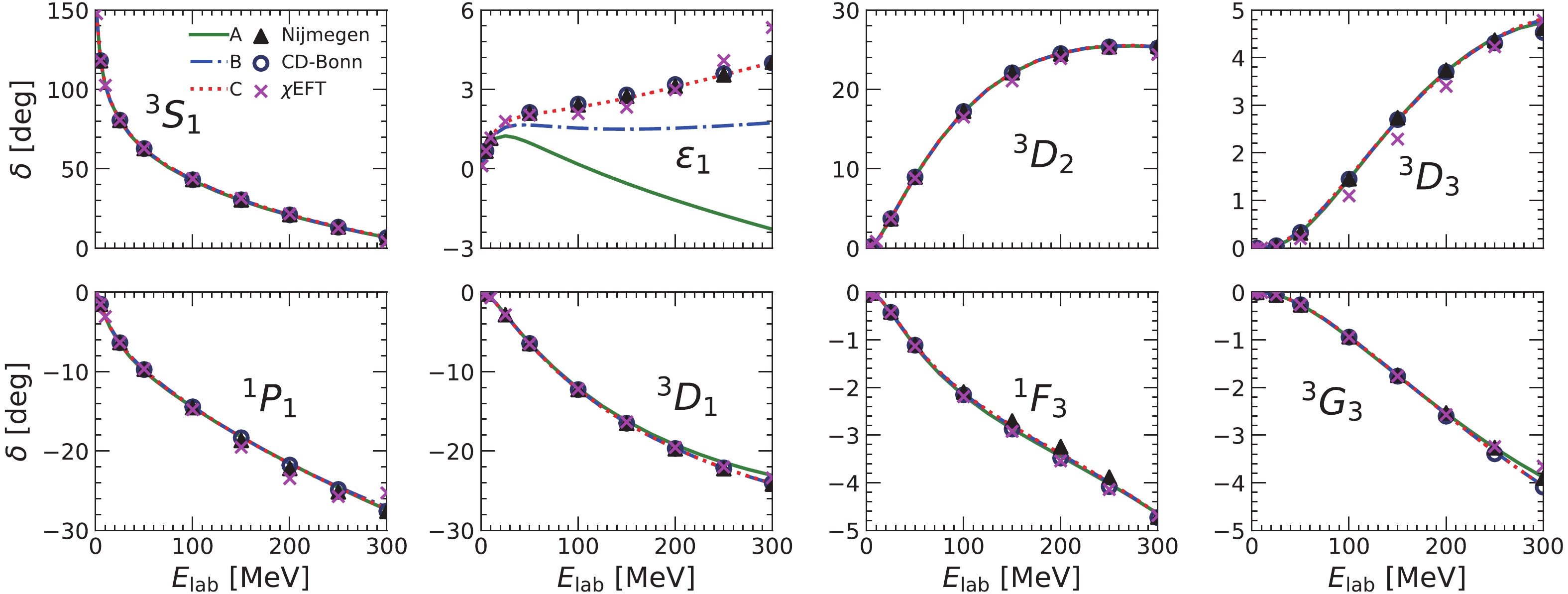
Figure 6. (color online) The
$np\; (T = 0)$ phase shifts and mixing parameters for different partial waves ($J\leqslant 3$ ). The triangles, open circles and crosses represent the phase shifts from Nijmegen PWA, the CD-Bonn potential, and the chiral N4LO potential by Entem et al., respectively.As an example, the coupling constants and masses of the
$ \sigma_1 $ and$ \sigma_2 $ mesons for the pp, nn and np components of the pvCD-Bonn C potential are listed up to the total angular momentum$ J = 4 $ in Table 2. Both cut-off momenta of the$ \sigma_1 $ and$ \sigma_2 $ mesons are taken as$ \Lambda_{\sigma_1,\; \sigma_2} = 2500 $ MeV. The blank denotes that there is no meson contribution. The detailed values of the phase shifts for the pp, nn, np scattering are tabulated in Tables 3-6. For all channels whose total angular momenta are larger than$ J = 4 $ , only one scalar meson is considered. Its mass and coupling constant are$ m_{\sigma} = 452 $ MeV,$ g^2_\sigma/4\pi = 2.3 $ for pvCD-Bonn B, C, and$ m_{\sigma} = 470 $ MeV,$ g^2_\sigma/4\pi = 4.3 $ for pvCD-Bonn A, following Ref. [29]. The coupling constants and phase shifts for the pvCD-Bonn A and B potentials are shown in detail in Appendix A. Finally,$ \chi^2 $ for the pvCD-Bonn A, B, C potentials are respectively$ 3.55\times 10^{-3}, \; 1.85\times 10^{-3} $ and$ 2.24\times 10^{-4} $ for the pp interaction, and$ 8.06\times 10^{-2}, $ $ 1.03\times 10^{-2} $ and$ 2.65\times 10^{-4} $ for the$ np(T = 0) $ interaction.$g^2_{\sigma_1}/4\pi$ 

$g^2_{\sigma_2}/4\pi$ 

$g^2_{\sigma_1}/4\pi$ 

$g^2_{\sigma_2}/4\pi$ 

$g^2_{\sigma_1}/4\pi$ 

$g^2_{\sigma_2}/4\pi$ 

$m_{\sigma_1}$ 

$m_{\sigma_2}$ 

pp np nn $^1S_0$ 

5.17 4.00 4.87 10.40 5.19 3.92 470 1225 $^3P_0$ 

4.32 38.04 4.32 27.08 4.34 36.15 500 1225 $^1P_1$ 

1.43 73.51 400 1225 $^3P_1$ 

2.29 70.04 2.26 69.76 2.29 73.00 424 1225 $^3D_1$ 

2.56 12.43 452 793 $^3S_1$ 

2.29 1.42 452 793 $^1D_2$ 

2.20 202.55 2.21 201.53 2.25 198.42 400 1225 $^3D_2$ 

0.67 59.26 350 1225 $^3F_2$ 

1.80 31.65 1.68 35.54 1.78 32.32 424 793 $^3P_2$ 

3.29 29.33 3.28 29.48 3.29 29.32 452 1225 $^1F_3$ 

0.90 400 $^3F_3$ 

2.70 45.81 2.82 43.50 2.70 45.81 452 793 $^3G_3$ 

1.68 350 $^3D_3$ 

1.52 350 $^1G_4$ 

3.90 3.90 3.90 452 $^3G_4$ 

3.90 452 $^3H_4$ 

3.36 3.36 3.36 452 $^3F_4$ 

3.80 3.80 3.80 452 Table 2. Parameters of
$\sigma_1$ and$\sigma_2$ for pvCD-Bonn C. Blanks indicate that the corresponding parameters are zero. The meson masses are in units of MeV.$T_{\rm lab}$ /MeV

$^1S_0$ 

$^3P_0$ 

$^3P_1$ 

$^1D_2$ 

$^3P_2$ 

$\varepsilon_2$ 

$^3F_2$ 

$^3F_3$ 

$^1G_4$ 

$^3F_4$ 

1 32.77 0.13 −0.08 0.00 0.01 0.00 0.00 −0.00 0.00 0.00 5 54.85 1.59 −0.90 0.04 0.22 −0.05 0.00 −0.01 0.00 0.00 10 55.22 3.75 −2.05 0.17 0.66 −0.20 0.01 −0.03 0.00 0.00 25 48.69 8.68 −4.90 0.70 2.50 −0.82 0.11 −0.23 0.04 0.02 50 38.94 11.72 −8.30 1.70 5.83 −1.73 0.34 −0.69 0.15 0.12 100 24.95 9.62 −13.31 3.74 10.94 −2.75 0.83 −1.49 0.41 0.51 150 14.76 4.72 −17.49 5.62 13.95 −3.02 1.20 −2.05 0.68 1.05 200 6.59 −0.51 −21.26 7.23 15.66 −2.90 1.41 −2.41 0.94 1.64 250 −0.30 −5.61 −24.73 8.55 16.62 −2.57 1.44 −2.65 1.21 2.21 300 −6.27 −10.49 −27.93 9.60 17.11 −2.13 1.29 −2.81 1.48 2.71 Table 3. pp phase shifts for different partial waves, predicted by pvCD-Bonn C.
$T_{\rm lab}$ /MeV

$^1P_1$ 

$^3S_1$ 

$\varepsilon_1$ 

$^3D_1$ 

$^3D_2$ 

$^1F_1$ 

$^3D_3$ 

$\varepsilon_3$ 

$^3F_3$ 

$^3G_4$ 

1 −0.19 147.76 0.10 −0.01 0.01 0.00 0.00 0.00 0.00 0.00 5 −1.50 118.19 0.67 −0.18 0.22 −0.01 0.00 0.01 0.00 0.00 10 −3.08 102.61 1.15 −0.68 0.85 −0.07 0.01 0.08 0.00 0.01 25 −6.42 80.58 1.76 −2.80 3.73 −0.42 0.07 0.55 −0.05 0.17 50 −9.81 62.66 2.04 −6.43 8.98 −1.10 0.38 1.61 −0.26 0.72 100 −14.43 43.02 2.33 −12.24 17.22 −2.12 1.48 3.48 −0.93 2.16 150 −18.23 30.51 2.67 −16.47 22.08 −2.80 2.69 4.83 −1.74 3.63 200 −21.60 21.09 3.09 −19.67 24.54 −3.39 3.69 5.76 −2.56 5.01 250 −24.60 13.46 3.55 −22.15 25.47 −3.99 4.41 6.39 −3.35 6.26 300 −27.28 6.99 4.02 −24.11 25.47 −4.65 4.82 6.82 −4.07 7.38 Table 6.
$np\; (T = 0)$ phase shifts for different partial waves, predicted by pvCD-Bonn C.$T_{\rm lab}$ /MeV

$^1S_0$ 

$^3P_0$ 

$^3P_1$ 

$^1D_2$ 

$^3P_2$ 

$\varepsilon_2$ 

$^3F_2$ 

$^3F_3$ 

$^1G_4$ 

$^3F_4$ 

1 57.40 0.21 −0.12 0.00 0.02 0.00 0.00 −0.00 0.00 0.00 5 60.91 1.86 −1.04 0.05 0.27 −0.06 0.00 −0.01 0.00 0.00 10 57.76 4.11 −2.24 0.18 0.76 −0.22 0.01 −0.04 0.00 0.00 25 49.07 8.98 −5.13 0.74 2.71 −0.85 0.11 −0.24 0.04 0.02 50 38.64 11.73 −8.54 1.77 6.14 −1.76 0.35 −0.70 0.16 0.12 100 24.40 9.45 −13.55 3.86 11.29 −2.75 0.84 −1.51 0.42 0.52 150 14.13 4.51 −17.74 5.78 14.30 −3.00 1.20 −2.06 0.68 1.07 200 5.94 −0.78 −21.50 7.41 15.99 −2.86 1.39 −2.42 0.95 1.70 250 −0.95 −5.88 −24.96 8.73 16.93 −2.51 1.39 −2.65 1.23 2.24 300 −6.93 −10.69 −28.14 9.77 17.40 −2.06 1.21 −2.80 1.50 2.74 Table 4. nn phase shifts for different partial waves, predicted by pvCD-Bonn C.
$T_{\rm lab}$ /MeV

$^1S_0$ 

$^3P_0$ 

$^3P_1$ 

$^1D_2$ 

$^3P_2$ 

$\varepsilon_2$ 

$^3F_2$ 

$^3F_3$ 

$^1G_4$ 

$^3F_4$ 

1 62.10 0.18 −0.11 0.00 0.02 0.00 0.00 −0.00 0.00 0.00 5 63.69 1.62 −0.93 0.04 0.26 −0.05 0.00 −0.00 0.00 0.00 10 60.03 3.64 −2.05 0.16 0.72 −0.18 0.01 −0.03 0.00 0.00 25 50.95 8.14 −4.85 0.68 2.58 −0.76 0.09 −0.20 0.03 0.02 50 40.45 10.76 −8.25 1.71 5.89 −1.65 0.31 −0.62 0.13 0.11 100 26.32 8.54 −13.33 3.83 10.94 −2.66 0.76 −1.38 0.38 0.48 150 16.22 3.67 −17.58 5.77 13.92 −2.95 1.11 −1.91 0.66 1.01 200 8.18 −1.57 −21.40 7.42 15.63 −2.84 1.31 −2.27 0.93 1.60 250 1.44 −6.65 −24.91 8.76 16.59 −2.52 1.33 −2.51 1.21 2.16 300 −4.41 −11.43 −28.14 9.82 17.08 −2.09 1.18 −2.68 1.49 2.65 Table 5.
$np\; (T = 1)$ phase shifts for different partial waves, predicted by pvCD-Bonn C.The tensor force in the OBE potential is generated not only by the pion but also by the
$ \rho $ and$ \omega $ mesons. In Fig. 7, the half-on-shell matrix elements for the pion,$ \omega $ and$ \rho $ mesons for the pvCD-Bonn A, B, C potentials in the coupled channels$ ^3S_1 $ -$ ^3D_1 $ and$ ^3P_2 $ -$ ^3F_2 $ are plotted for the on-shell momentum$ q' = 265 $ MeV. The pion provides the largest attractive contribution in the$ ^3S_1 $ -$ ^3D_1 $ channel, while the tensor component of the$ \rho $ meson is repulsive. The$ \omega $ meson also gives slight attraction. In the$ ^3P_2 $ -$ ^3F_2 $ channel, the situations for the pion and$ \rho $ meson are opposite. The$ \omega $ meson still provides a slightly attractive contribution.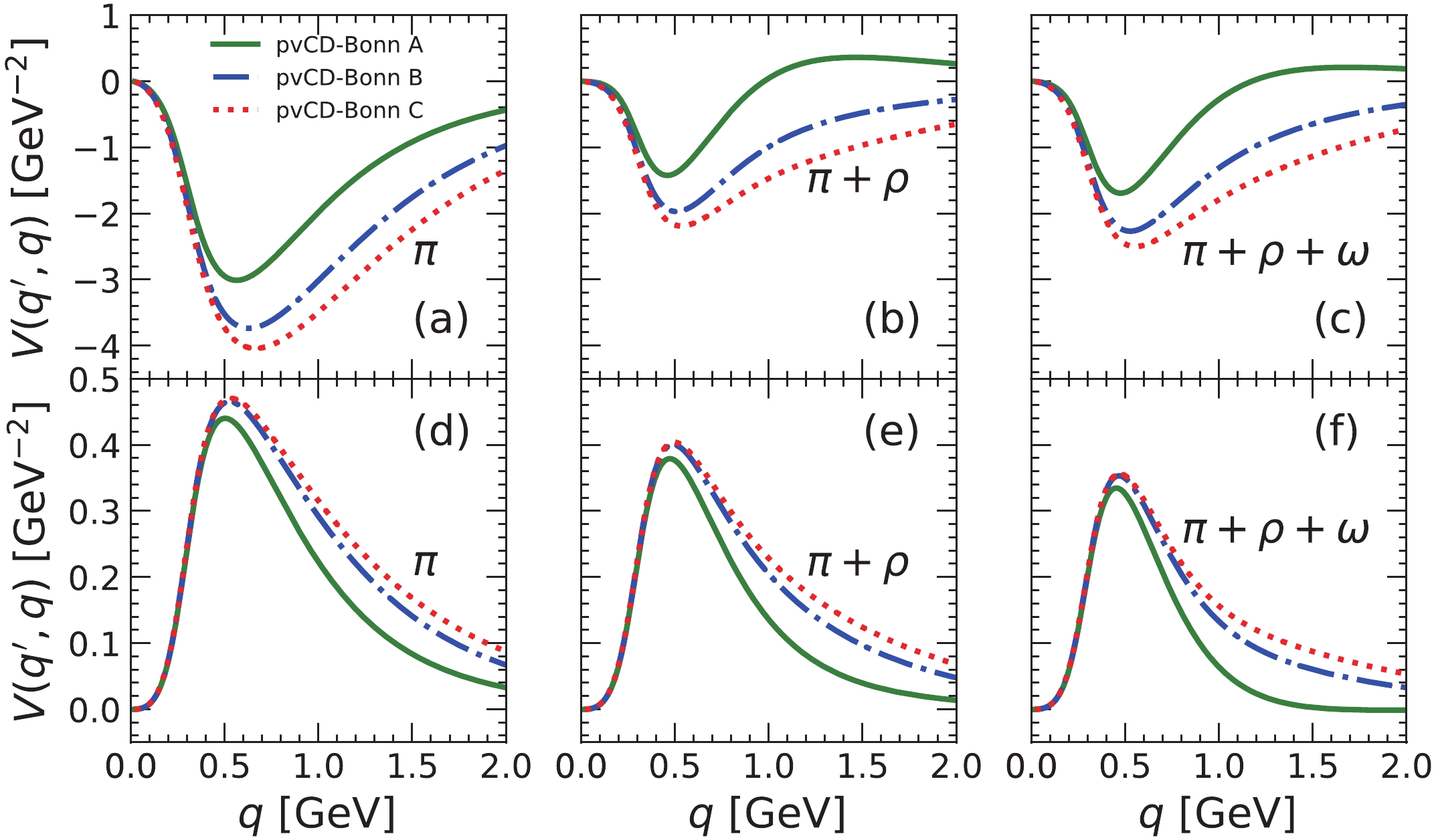
Figure 7. (color onlinr) The off-shell
$^3S_1$ -$^3D_1$ (panel above) and$^3P_2$ -$^3F_2$ (panel behind) potentials. The half-on-shell momentum is fixed at$q' = 265$ MeV. -
Once the NN potentials are determined, they can be immediately applied to obtain the lower energy NN scattering parameters, such as the scattering length, effective range, and the binding properties of the deuteron, which have been accurately measured. At low laboratory energy, the anti-tangent values of the phase shifts can be expanded as function of momentum. The coefficients of the first two terms are defined as the scattering length a and the effective range r. Their values for the
$ ^1S_0 $ and$ ^3S_1 $ channels of pp, nn, and np scattering for the pvCD-Bonn A, B, C potentials are given in Table 7. The corresponding experimental results are also shown for comparison. It can be seen that the theoretical calculations for these potentials with PV pion-nucleon coupling are consistent with the experiment results.A B C experiment references $a^N_{pp}$ 

−17.325 −17.292 −17.255 $r^N_{pp}$ 

2.820 2.813 2.809 $a_{np}$ 

−23.711 −23.757 −23.734 −23.74±0.02 [41] $r_{np}$ 

2.649 2.649 2.646 2.77±0.05 [41] $a_t$ 

5.432 5.417 5.417 5.419±0.007 [41] $r_t$ 

1.773 1.753 1.757 1.753±0.008 [41] $a_{nn}$ 

−18.806 −18.744 −18.741 −18.9±0.4 [42, 43] $r_{nn}$ 

2.795 2.786 2.784 2.75±0.11 [44] Table 7. The low-energy NN scattering parameters: the scattering length a and the effective range r (in units of fm). The Coulomb effects are excluded in these data.
The deuteron is the only bound state of the np system. It was found that to describe reasonably its quadrupole moment, the deuteron wave functions should be a combination of the S and D states. The solution for the deuteron bound state corresponds to a pole in the scattering equation. Therefore, the deuteron wave functions can be obtained from the scattering equation by introducing the experimental value of the deuteron binding energy,
$ B_d = 2.224575 $ MeV [40]. From the wave function, the ratio of the$ D/S $ states$ \eta $ , the asymptotic S-state normalization constant$ A_S $ , the root-mean-square radius of the deuteron$ r_d $ , the quadrupole moment$ Q_d $ , and the D-state probability$ P_D $ , as predicted by the pvCD-Bonn A, B, C potentials, are listed in Table 8. Apart from the D-state probability, the other quantities can be measured or extracted from the experiments. Although these three potentials have different tensor components, they provide similar description of the properties of the deuteron, and are consistent with the experimental data or the empirical values. It should be noted that the quadruple moment for the pvCD-Bonn C potential,$ Q_d = 0.273 $ fm2 is closer to the experimental data than for the CD-Bonn potential with PS coupling,$ Q_d = 0.270 $ fm2. Furthermore, the pvCD-Bonn C potential has the strongest tensor component with PD = 6.06%, as shown in Fig. 7. In Ref. [30], Caia et al. mentioned that$ P_D $ is 0.4%-0.5% higher for PV coupling than for PS coupling. In this work,$ P_D $ for the pvCD-Bonn C potential is much larger than for the original CD-Bonn potential (4.85%).$ P_D $ is strongly related to the tensor force, to which the pion and$ \omega,\; \rho $ mesons contribute in the CD-Bonn potential. To compare the difference between the PV and PS couplings, the coupling constants and the cutoffs for the pvCD-Bonn C potential and the original CD-Bonn potential are taken in this work to have the same value, while these parameters were used in the work of Caia et al. to fit the phase shifts. Therefore, the differences of$ P_D $ for the pvCD-Bonn C potential and the original CD-Bonn potential are completely due to the PV and PS couplings.Table 8. The predicted deuteron properties for the pvCD-Bonn A, B, C potentials.
$\eta$ is the$D/S$ ratio,$A_s$ is the asymptotic S-state normalization in${\rm{fm}}^{\frac{1}{2}}$ ,$r_d$ is the deuteron radius in fm,$Q_d$ is the quadrupole momentum in fm2 , and$P_D$ is the D-state probability.In Fig. 8, the wave functions of the deuteron in the S-state,
$ u(r) $ , and D-state,$ w(r) $ , for the pvCD-Bonn A, B, C potentials are shown in coordinate space. These wave functions were obtained first in the momentum representation of the Lippmann-Schwinger equation. They were transformed into the coordinate space by Fourier transformation. For the S-state, the wave functions for the three potentials are almost identical. There are significant differences in the wave functions of the D-state in the intermediate range, between$ 1-2 $ fm. This is just the interaction range of the tensor force. The wave function of the pvCD-Bonn C potential has the largest amplitude in the D-state, which produces the strongest D-state probability.
Figure 8. (color online) The predicted normalized deuteron wave functions in the configuration space for pvCD-Bonn A, B, C.
The deuteron wave functions squared in the momentum space for the
$ L = 0 $ and$ L = 2 $ states are shown in Fig. 9 for our three potentials. They are very important for calculating the electromagnetic form factors of the deuteron [49]. There is a rapid decrease of$ |\psi(k)|^2 $ in the S-state around$ k = 2 $ fm-1, due to the strong repulsion of the NN interaction at short distances, which changes the sign of the deuteron wave function. Actually, the behavior of the deuteron wave functions is similar to the other realistic NN interactions [49, 50]. In the region of small momenta, the wave functions for the pvCD-Bonn A, B, C potentials are very similar, while there are clear differences for high momenta, which correspond to the short-range NN interactions.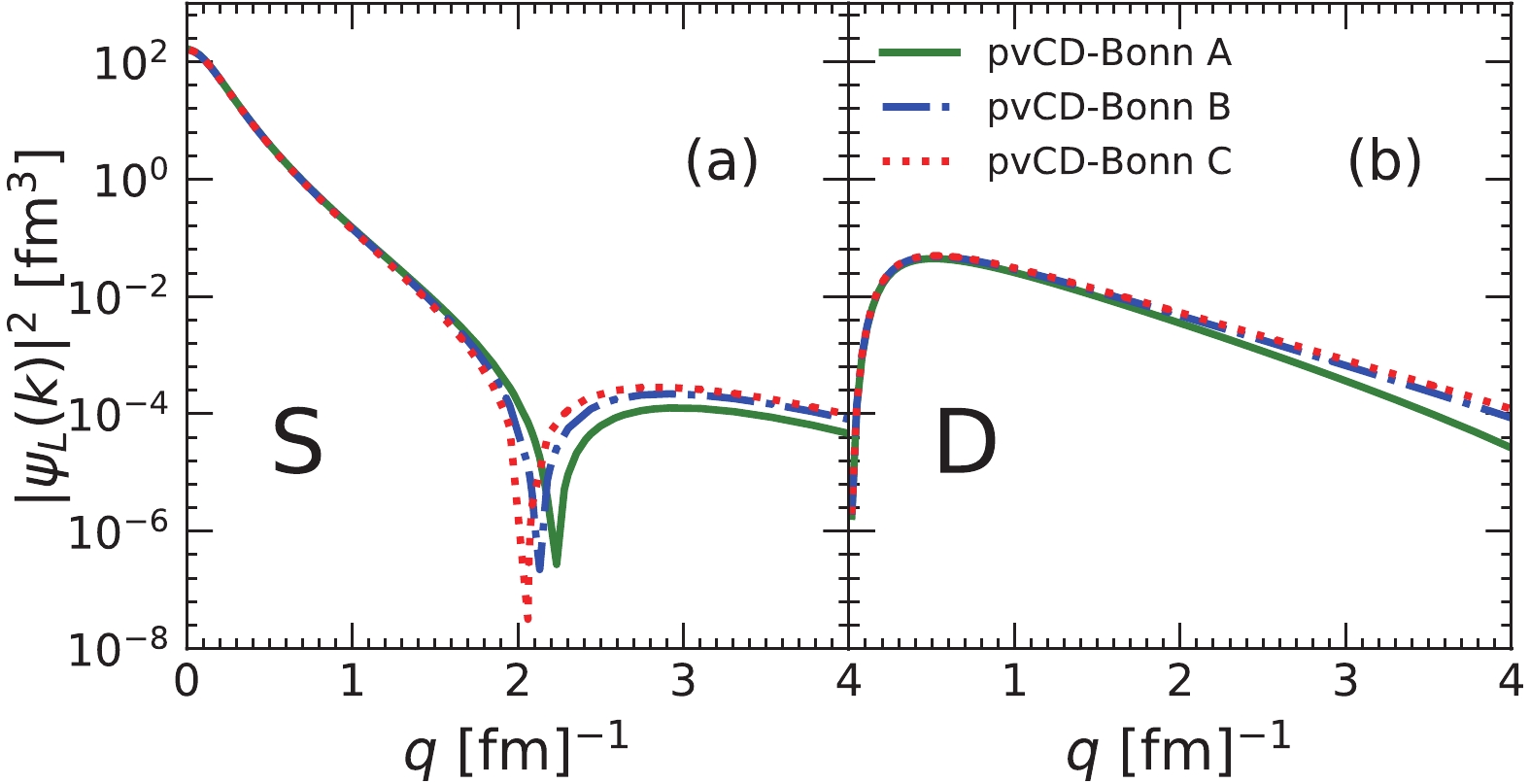
Figure 9. (color online) The predicted deuteron wave function squared for the S- and D-states in the momentum space for pvCD-Bonn A, B, C.
Generally speaking, the pvCD-Bonn C potential perfectly describes the phase shifts from Nijmegen PWA and generates the best properties of the deuteron. Its D-state probability is higher than for the CD-Bonn potential and the latest N4LO chiral potentials, whose
$ P_D $ are all around 4%. Actually, the NN potentials with PV coupling usually generate a larger$ P_D $ , which was shown for the Bonn A, B, C potentials in the work by Caia et al. [30]. -
Based on the high-precision CD-Bonn potential, three revised NN potentials were proposed, called the pvCD-Bonn A, B, C potentials, where the pion-nucleon coupling was taken as pseudovector instead of the original pseudoscalar. Besides the pion, the
$ \omega,\; \rho $ and two scalar mesons$ \sigma_1 $ and$ \sigma_2 $ are also included in these potentials. To describe more precisely the charge symmetry breaking and charge independence breaking in the phase shifts from Nijmegen PWA, the coupling constants of the$ \sigma_1 $ and$ \sigma_2 $ mesons were fitted independently for each partial wave. The strengths of the one-pion-exchange component in the pvCD-Bonn A, B, C potentials are distinguished by different cut-off momenta.The phase shifts from the three potentials in the non-coupled channels are consistent with Nijmegen PWA. The only differences appear in the mixing parameters of the coupled channels due to different tensor components. The pvCD-Bonn C potential describes very well all phase shifts from Nijmegen PWA in all channels up to
$ J = 4 $ , which include the strongest pion components. The potentials generate similar properties of the deuteron, such as the$ D/S $ -state ratio, root-mean-square radius and the quadrupole moment, while the D-state probabilities for the pvCD-Bonn A, B, C potentials are different, and are respectively 4.22%, 5.45%, 6.05%.The original CD-Bonn potential has been applied to many aspects of nuclear physics and has obtained great achievements. However, it is very difficult to use in the relativistic framework due to the pseudoscalar pion-nucleon coupling, which generates a large attractive contribution in the nucleon-antinucleon excitation. Therefore, three charge-dependent one-boson-exchange potentials were proposed in this work with pion-nucleon pseudovector coupling. They could be widely used for calculating various nuclear many-body problems in the relativistic framework, and for investigating the relativistic and tensor force effects.
-
The coupling constants and masses of
$ \sigma_1 $ and$ \sigma_2 $ mesons for partial waves up to$ J = 4 $ and the pvCD-Bonn A and pvCD-Bonn B potentials are listed in Tables A1 and A2. The corresponding phase shifts for$ pp,\; nn, $ and np are given in Tables A3–A10.$g^2_{\sigma_1}/4\pi$ 

$g^2_{\sigma_2}/4\pi$ 

$g^2_{\sigma_1}/4\pi$ 

$g^2_{\sigma_2}/4\pi$ 

$g^2_{\sigma_1}/4\pi$ 

$g^2_{\sigma_2}/4\pi$ 

$m_{\sigma_1}$ 

$m_{\sigma_2}$ 

pp np nn $^1S_0$ 

5.17 2.13 4.65 4.35 5.19 2.10 470 793 $^3P_0$ 

6.37 8.53 6.38 7.98 6.39 8.52 560 793 $^1P_1$ 

0.64 11.16 350 793 $^3P_1$ 

0.93 10.123 0.93 9.84 0.93 10.12 350 793 $^3D_1$ 

$^3S_1$ 

2.20 9.89 452 793 $^1D_2$ 

0.93 32.19 0.94 32.00 0.93 32.35 350 793 $^3D_2$ 

1.27 15.22 452 793 $^3F_2$ 

0.40 59.78 0.53 45.06 0.39 60.69 350 793 $^3P_2$ 

0.93 14.69 0.92 14.76 0.93 14.69 350 793 $^1F_3$ 

0.99 350 $^3F_3$ 

1.74 36.28 1.68 38.02 1.77 36.5 400 793 $^3G_3$ 

2.51 400 $^3D_3$ 

1.6 1.8 400 793 $^1G_4$ 

4.7 4.9 4.7 470 $^3G_4$ 

2.6 470 $^3H_4$ 

4.5 4.5 4.5 470 $^3F_4$ 

4.5 4.5 4.5 470 Table A1. Parameters of
$\sigma_1$ and$\sigma_2$ adopted in pvCD-Bonn A potential. Blanks indicate the corresponding parameters taken as zero. Meson masses in unit MeV.$g^2_{\sigma_1}/4\pi$ 

$g^2_{\sigma_2}/4\pi$ 

$g^2_{\sigma_1}/4\pi$ 

$g^2_{\sigma_2}/4\pi$ 

$g^2_{\sigma_1}/4\pi$ 

$g^2_{\sigma_2}/4\pi$ 

$m_{\sigma_1}$ 

$m_{\sigma_2}$ 

pp np nn $^1S_0$ 

5.19 5.30 4.89 11.54 5.20 5.58 470 1225 $^3P_0$ 

5.07 43.42 5.06 34.10 5.09 42.87 520 1225 $^1P_1$ 

0.74 89.73 350 1225 $^3P_1$ 

2.36 52.46 2.42 40.79 2.38 52.09 424 1225 $^3D_1$ 

1.88 1.30 452 793 $^3S_1$ 

1.83 6.74 452 793 $^1D_2$ 

2.19 208.07 2.20 206.78 2.23 32.35 400 1225 $^3D_2$ 

1.45 21.33 424 1225 $^3F_2$ 

1.87 23.97 1.86 24.09 1.86 23.79 424 793 $^3P_2$ 

3.28 30.14 3.26 30.45 3.29 30.08 452 1225 $^1F_3$ 

0.90 350 $^3F_3$ 

3.01 40.82 2.96 41.32 3.02 40.90 452 793 $^3G_3$ 

0.90 350 $^3D_3$ 

0.80 5.54 350 793 $^1G_4$ 

3.83 3.85 3.83 452 $^3G_4$ 

3.60 470 $^3H_4$ 

3.74 3.78 3.74 452 $^3F_4$ 

3.74 3.78 3.74 452 Table A2. Parameters of
$\sigma_1$ and$\sigma_2$ adopted in pvCD-Bonn B potential. Blanks indicate the corresponding parameters taken as zero. Meson masses in unit MeV.$T_{\rm lab}$ /MeV

$^1S_0$ 

$^3P_0$ 

$^3P_1$ 

$^1D_2$ 

$^3P_2$ 

$\varepsilon_2$ 

$^3F_2$ 

$^3F_3$ 

$^1G_4$ 

$^3F_4$ 

1 32.82 0.14 −0.08 0.00 0.02 0.00 0.00 −0.00 0.00 0.00 5 54.84 1.60 −0.90 0.04 0.24 −0.05 0.00 −0.01 0.00 0.00 10 55.18 3.78 −2.04 0.17 0.71 −0.21 0.01 −0.03 0.00 0.00 25 48.63 8.70 −4.89 0.71 2.62 −0.83 0.11 −0.23 0.04 0.02 50 38.89 11.71 −8.29 1.72 5.93 −1.76 0.35 −0.69 0.15 0.12 100 24.93 9.61 −13.34 3.74 10.89 −2.74 0.82 −1.49 0.42 0.50 150 14.78 4.73 −17.53 5.62 13.89 −2.95 1.16 −2.04 0.68 1.03 200 6.65 −0.49 −21.27 7.25 15.67 −2.74 1.36 −2.43 0.94 1.63 250 −0.20 −5.60 −24.68 8.58 16.70 −2.31 1.40 −2.72 1.21 2.21 300 −6.12 −10.50 −27.82 9.59 17.20 −1.77 1.29 −2.96 1.48 2.74 Table A3. pp phase shifts in different partial waves, predicted by pvCD-Bonn A.
$T_{\rm lab}$ /MeV

$^1P_1$ 

$^3S_1$ 

$\varepsilon_1$ 

$^3D_1$ 

$^3D_2$ 

$^1F_1$ 

$^3D_3$ 

$\varepsilon_3$ 

$^3F_3$ 

$^3G_4$ 

1 −0.19 147.76 0.10 −0.01 0.01 0.00 0.00 0.00 0.00 0.00 5 −1.50 118.21 0.64 −0.18 0.22 −0.01 0.00 0.01 0.00 0.00 10 −3.07 102.65 1.08 −0.68 0.85 −0.07 0.01 0.08 0.00 0.01 25 −6.38 80.65 1.57 −2.80 3.73 −0.42 0.07 0.56 −0.05 0.17 50 −9.75 62.72 1.65 −6.43 8.97 −1.11 0.38 1.62 −0.26 0.72 100 −14.41 43.04 1.54 −12.24 17.22 −2.13 1.48 3.51 −0.93 2.18 150 −18.24 30.45 1.50 −16.47 22.12 −2.82 2.69 4.86 −1.74 3.65 200 −21.58 20.96 1.54 −19.67 24.58 −3.40 3.69 5.79 −2.56 5.02 250 −24.50 13.25 1.63 −22.15 25.48 −3.99 4.40 6.42 −3.45 6.27 300 −27.07 6.71 1.74 −24.11 25.38 −4.65 4.80 6.85 −4.07 7.38 Table A10.
$np\; (T = 0)$ phase shifts in different partial waves, predicted by pvCD-Bonn B.$T_{\rm lab}$ /MeV

$^1S_0$ 

$^3P_0$ 

$^3P_1$ 

$^1D_2$ 

$^3P_2$ 

$\varepsilon_2$ 

$^3F_2$ 

$^3F_3$ 

$^1G_4$ 

$^3F_4$ 

1 57.45 0.21 −0.12 0.00 0.03 0.00 0.00 −0.00 0.00 0.00 5 60.89 1.87 −1.04 0.05 0.30 −0.06 0.00 −0.01 0.00 0.00 10 57.71 4.14 −2.24 0.19 0.82 −0.22 0.02 −0.04 0.00 0.00 25 49.01 9.00 −5.12 0.75 2.84 −0.86 0.11 −0.24 0.04 0.02 50 38.59 11.71 −8.54 1.78 6.23 −1.79 0.35 −0.71 0.16 0.12 100 24.38 9.43 −13.61 3.83 11.23 −2.75 0.82 −1.50 0.42 0.51 150 14.15 4.51 −17.82 5.75 14.23 −2.93 1.17 −2.05 0.69 1.06 200 6.00 −0.76 −21.57 7.40 15.99 −2.70 1.36 −2.43 0.95 1.66 250 −0.84 −5.87 −24.99 8.75 16.98 −2.25 1.40 −2.71 1.22 2.25 300 −6.78 −10.70 −28.14 9.77 17.47 −1.70 1.29 −2.95 1.49 2.78 Table A4. nn phase shifts in different partial waves, predicted by pvCD-Bonn A.
$T_{\rm lab}$ /MeV

$^1S_0$ 

$^3P_0$ 

$^3P_1$ 

$^1D_2$ 

$^3P_2$ 

$\varepsilon_2$ 

$^3F_2$ 

$^3F_3$ 

$^1G_4$ 

$^3F_4$ 

1 62.07 0.18 −0.11 0.00 0.02 0.00 0.00 −0.00 0.00 0.00 5 63.67 1.63 −0.93 0.04 0.28 −0.05 0.00 −0.00 0.00 0.00 10 60.03 3.66 −2.04 0.16 0.77 −0.19 0.01 −0.03 0.00 0.00 25 50.98 8.14 −4.82 0.70 2.68 −0.77 0.09 −0.20 0.03 0.02 50 40.52 10.73 −8.22 1.73 5.94 −1.67 0.32 −0.62 0.14 0.10 100 26.43 8.51 −13.33 3.83 10.82 −2.64 0.77 −1.38 0.39 0.47 150 16.34 3.66 −17.59 5.77 13.79 −2.86 1.10 −1.91 0.66 1.00 200 8.32 −1.56 −21.38 7.44 15.56 −2.65 1.27 −2.27 0.94 1.59 250 1.58 −6.64 −24.84 8.78 16.59 −2.22 1.26 −2.51 1.22 2.17 300 −4.26 −11.43 −28.01 9.79 17.11 −1.68 1.09 −2.68 1.50 2.69 Table A5.
$np\; (T = 1)$ phase shifts in different partial waves, predicted by pvCD-Bonn A.$T_{\rm lab}$ /MeV

$^1P_1$ 

$^3S_1$ 

$\varepsilon_1$ 

$^3D_1$ 

$^3D_2$ 

$^1F_1$ 

$^3D_3$ 

$\varepsilon_3$ 

$^3F_3$ 

$^3G_4$ 

1 −0.19 147.69 0.10 −0.01 0.01 0.00 0.00 0.00 0.00 0.00 5 −1.53 118.00 0.59 −0.18 0.23 −0.01 0.00 0.01 0.00 0.00 10 −3.13 102.36 0.96 −0.67 0.86 −0.07 0.01 0.08 0.00 0.01 25 −6.51 80.23 1.24 −2.77 3.76 −0.42 0.06 0.56 −0.05 0.17 50 −9.92 62.20 0.98 −6.38 9.00 −1.12 0.34 1.64 −0.26 0.73 100 −14.49 42.50 0.17 −12.11 17.21 −2.17 1.45 3.56 −0.94 2.20 150 −18.23 29.99 −0.55 −16.22 22.09 −2.87 2.70 4.94 −1.75 3.67 200 −21.56 20.63 −1.19 −19.22 24.55 −3.44 3.72 5.89 −2.54 5.02 250 −24.60 13.08 −1.76 −21.43 25.44 −4.02 4.40 6.54 −3.26 6.23 300 −27.40 6.73 −2.29 −23.07 25.34 −4.65 4.75 6.98 −3.88 7.29 Table A6.
$np\; (T = 0)$ phase shifts in different partial waves, predicted by pvCD-Bonn A.$T_{\rm lab}$ /MeV

$^1S_0$ 

$^3P_0$ 

$^3P_1$ 

$^1D_2$ 

$^3P_2$ 

$\varepsilon_2$ 

$^3F_2$ 

$^3F_3$ 

$^1G_4$ 

$^3F_4$ 

1 32.80 0.14 −0.08 0.00 0.01 0.00 0.00 −0.00 0.00 0.00 5 54.85 1.59 −0.90 0.04 0.22 −0.05 0.00 −0.01 0.00 0.00 10 55.21 3.76 −2.05 0.17 0.66 −0.20 0.01 −0.03 0.00 0.00 25 48.67 8.69 −4.91 0.70 2.51 −0.82 0.11 −0.23 0.04 0.02 50 38.92 11.72 −8.30 1.71 5.83 −1.74 0.35 −0.69 0.15 0.12 100 24.94 9.62 −13.30 3.74 10.95 −2.75 0.83 −1.50 0.41 0.50 150 14.77 4.73 −17.49 5.62 13.97 −3.01 1.19 −2.05 0.68 1.04 200 6.62 −0.50 −21.28 7.23 15.69 −2.86 1.39 −2.40 0.94 1.63 250 −0.25 −5.60 −24.77 8.55 16.65 −2.50 1.39 −2.64 1.21 2.19 300 −6.20 −10.49 −28.01 9.60 17.15 −2.03 1.22 −2.81 1.47 2.68 Table A7. pp phase shifts in different partial waves, predicted by pvCD-Bonn B.
$T_{\rm lab}$ /MeV

$^1S_0$ 

$^3P_0$ 

$^3P_1$ 

$^1D_2$ 

$^3P_2$ 

$\varepsilon_2$ 

$^3F_2$ 

$^3F_3$ 

$^1G_4$ 

$^3F_4$ 

1 57.40 0.21 −0.12 0.00 0.02 0.00 0.00 −0.00 0.00 0.00 5 60.90 1.86 −1.04 0.05 0.27 −0.06 0.00 −0.01 0.00 0.00 10 57.75 4.12 −2.24 0.18 0.76 −0.22 0.01 −0.04 0.00 0.00 25 49.06 8.98 −5.13 0.74 2.72 −0.85 0.11 −0.24 0.04 0.02 50 38.66 11.72 −8.53 1.77 6.14 −1.78 0.35 −0.71 0.16 0.12 100 24.44 9.44 −13.53 3.86 11.30 −2.76 0.84 −1.52 0.42 0.52 150 14.21 4.51 −17.73 5.78 14.31 −2.99 1.20 −2.06 0.69 1.06 200 6.05 −0.77 −21.52 7.40 16.00 −2.82 1.39 −2.42 0.95 1.65 250 −0.80 −5.88 −25.02 8.73 16.93 −2.44 1.39 −2.65 1.22 2.22 300 −6.75 −10.69 −28.26 9.78 17.40 −1.96 1.21 −2.81 1.49 2.71 Table A8. nn phase shifts in different partial waves, predicted by pvCD-Bonn B.
$T_{\rm lab}$ /MeV

$^1S_0$ 

$^3P_0$ 

$^3P_1$ 

$^1D_2$ 

$^3P_2$ 

$\varepsilon_2$ 

$^3F_2$ 

$^3F_3$ 

$^1G_4$ 

$^3F_4$ 

1 62.10 0.18 −0.11 0.00 0.02 0.00 0.00 −0.00 0.00 0.00 5 63.68 1.62 −0.93 0.04 0.25 −0.05 0.00 −0.00 0.00 0.00 10 60.02 3.64 −2.04 0.16 0.72 −0.19 0.01 −0.03 0.00 0.00 25 50.94 8.14 −4.83 0.69 2.57 −0.76 0.09 −0.20 0.03 0.02 50 40.44 10.75 −8.19 1.72 5.86 −1.66 0.31 −0.62 0.14 0.11 100 26.33 8.53 −13.24 3.83 10.89 −2.66 0.77 −1.38 0.39 0.48 150 16.26 3.67 −17.51 5.77 13.87 −2.93 1.12 −1.92 0.66 1.01 200 8.25 −1.56 −21.38 7.42 15.59 −2.80 1.30 −2.27 0.94 1.59 250 1.53 −6.64 −24.95 8.76 16.56 −2.45 1.29 −2.51 1.22 2.15 300 −4.28 −11.43 −28.27 9.82 17.07 −1.99 1.10 −2.68 1.50 2.65 Table A9.
$np\; (T = 1)$ phase shifts in different partial waves, predicted by pvCD-Bonn B. -
The BbS equation in this work was solved in the LSJ basis. Therefore, the matrix elements for the pvCD-Bonn potentials are expressed in the LSJ basis. There are many references where the one-boson-exchange (OBE) potentials in the LSJ basis are formulated in detail, such as Refs. [11, 12, 29]. From the quantum field theory, the OBE potentials are derived from the free nucleon scattering amplitudes as shown in Eq. (6), where the Dirac spinor is obtained by solving the free Dirac equation, and is normalized by
$ \bar{u}u = 1 $ ,$\tag{B1} u({{p}},\lambda ) = \sqrt {\frac{{M + E}}{{2M}}} \left( {\begin{array}{*{20}{c}} 1\\ {\frac{{{{\sigma}} \cdot {{p}}}}{{M + E}}} \end{array}} \right)|\lambda \rangle, $

(B13) where
$ |\lambda = \pm \displaystyle \frac{1}{2}\rangle $ is the spin wave function. Here, the anti-nucleon degree of freedom is neglected. The exact expressions for the$ \sigma $ meson, pion with pseudovector coupling, and$ \omega $ meson can be expanded in terms of the Dirac spinor as$\tag{B2} \begin{split} \bar{V}_\sigma ({ q}',{ q})& = -g_\sigma^2 \bar{u}({ q}')u({ q})\frac{1}{{ k}^2+m^2_\sigma} \bar{u}(-{ q}')u(-{ q}) \\ & = -g_\sigma^2\frac{W'W}{4M^2} \left(1-\frac{{\sigma}_1\cdot{ q}'}{W'} \frac{{\sigma}_1\cdot{ q}}{W}\right) \left(1-\frac{{\sigma}_2\cdot{ q}'}{W'} \frac{{\sigma}_2\cdot{ q}}{W}\right)\\ &\quad\times\frac{1}{{ k}^2+m_\sigma^2}, \end{split} $

(B14) $\tag{B3} \begin{split} \bar{V}^{{\rm pv}}_{\pi}({ q}',{ q}) & = -\frac{f^2_\pi}{m_\pi^2}\bar{u}({ q}')\gamma^5 {\gamma}\cdot { k}u({ q})\frac{1}{{ k}^2+m^2_\pi} \bar{u}(-{ q}')\gamma^5{\gamma}\cdot { k}u(-{ q}) \\ & = -\frac{f_\pi^2}{m_\pi^2}\frac{WW'}{4M^2}\left[ (E'-E+2M)\frac{{\sigma}_1\cdot{ q}'}{W'}- (E-E'+2M)\frac{{\sigma}_1\cdot{ q}}{W}\right] \\ &\quad \times\left[(E'-E+2M)\frac{{\sigma}_2\cdot{ q}'}{W'}- (E-E'+2M)\frac{{\sigma}_2\cdot{ q}}{W}\right]\\ &\quad\times\frac{1}{{ k}^2+m_\pi^2}, \end{split} $

(B15) $\tag{B4} \begin{split} \bar{V}_\omega({ q}',{ q}) & = g_\omega^2 \bar{u}({ q}')\gamma^\mu u({ q})\frac{1}{{ k}^2+m^2_\omega} \bar{u}(-{ q}')\gamma_\mu u(-{ q}) \\ & = g_\omega^2\frac{W'W}{4M^2} \left[ \left(1+\frac{{\sigma}_1\cdot{ q}'}{W'} \frac{{\sigma}_1\cdot{\bf q}}{W}\right) \left(1+\frac{{\sigma}_2\cdot{ q}'}{W'} \frac{{\sigma}_2\cdot{ q}}{W}\right) \right. \\ &\quad +\left.\left(\frac{{\sigma}_1\cdot{ q}'}{W'} {\sigma}_1+ {\sigma}_1\frac{{\sigma}_1 \cdot { q}}{W}\right) \left(\frac{{\sigma}_2\cdot{ q}'}{W'}{\sigma}_2+ {\sigma}_2 \frac{{\sigma}_2 \cdot { q}}{W}\right) \right]\\ &\quad\times\frac{1}{{ k}^2+m_\omega^2}, \end{split} $

(B16) where the wave functions of the spin and isospin operators are omitted, and
$ W' = E'+M $ and$ W = E+M $ . The expression for the$ \rho $ meson is more complicated than for the other mesons due to the tensor coupling:$\tag{B5} \begin{split} \bar{V}_\rho({ q}',{ q}) = & \bar{u}({ q}') \left[g_\rho\gamma_\mu +\frac{f_\rho}{2M_p}(\gamma_\mu{\gamma}\cdot{ k} -k_\mu)\right] u({ q}) \frac{1}{{ k}^2+m_\rho^2} \\ & \bar{u}(-{ q}') \left[g_\rho\gamma^\mu +\frac{f_\rho}{2M_p}(\gamma^\mu{\gamma}\cdot { k}-k^\mu)\right]u(-{ q}), \end{split} $

(B17) where
$ \gamma^\mu = (\gamma^0,{\gamma}) $ is the conventional gamma matrix, and$ k^\mu = (0,{ k}) $ is the relative four-momentum of the two interacting nucleons. The matrix element for the$ \rho $ meson (15) is divided into 3 parts,$ \bar{V}_\rho = \bar{V}_{vv} + \bar{V}_{vt} + \bar{V}_{tt} $ . The vector-vector coupling part is$ \bar{V}_{vv}({ q}',{ q}) = g_\rho^2 \bar{u}({ q}')\gamma^\mu u({ q})\frac{1}{{ k}^2+m^2_\rho} \bar{u}(-{ q}')\gamma_\mu u(-{ q}), $

which is identical to the
$ \omega $ meson potential (B2). The vector-tensor coupling is$\tag{B6} \begin{split} \bar{V}_{vt}({ q}',{ q}) =&\frac{g_\rho f_\rho}{2M_p} \left[ {\; \bar{u}({\bf q}')\gamma_\mu u({ q})\bar{u}(-{ q}') (\gamma^\mu {\gamma}\cdot { k}-k^\mu) u(-{ q})} \right.\\ & \left.{ +\bar{u}({ q}')(\gamma_\mu {\gamma}\cdot { k}-k_\mu)u({ q})\bar{u}(-{ q}')\gamma^\mu u(-{ q})} \right] \frac{1}{{ k}^2+m_\rho^2}. \end{split} $

(B18) The tensor-tensor coupling is written as,
$\tag{B7} \begin{split} \bar{V}_{tt}({ q}',{ q}) = &\frac{f_\rho^2}{4M_p^2} \bar{u}({ q}')(\gamma_\mu {\gamma}\cdot { k}-k_\mu)u({ q})\frac{1}{{ k}^2+m_\rho^2}\\ &\bar{u}(-{ q}')(\gamma^\mu {\gamma}\cdot { k}-k^\mu) u(-{ q}). \end{split} $

(B19) The full pvCD-Bonn potentials (9) are the sum of all meson contributions. In the above expressions, the spin structure of the Dirac spinor is strongly dependent on the spin wave functions of the in- and out- scattering states. The expectation values of the spin structure are calculated with the spin wave function. To simplify the computational process, the helicity representation is adopted, where the spin is quantized along the direction of initial and final momenta,
$ |\lambda\rangle $ . In principle, there are 16 terms for$ \langle\lambda'_1\lambda'_2|V({ q}', { q})|\lambda_1\lambda_2\rangle $ , since each helicity$ \lambda $ can be$ 1/2 $ or$ -1/2 $ . Due to parity conservation and time-reversal invariance in the scattering of two identical fermions, only six matrix elements are independent:$ \tag{B8} \begin{split} V^J_1(q',q) = &\langle ++|V^J(q',q)|++\rangle, \\ V^J_2(q',q) =& \langle ++|V^J(q',q)|--\rangle, \\ V^J_3(q',q) =& \langle +-|V^J(q',q)|+-\rangle, \\ V^J_4(q',q) = &\langle +-|V^J(q',q)|-+\rangle, \\ V^J_5(q',q) =& \langle ++|V^J(q',q)|+-\rangle, \\ V^J_6(q',q) =& \langle +-|V^J(q',q)|++\rangle, \end{split} $

(B20) where the momentum angle dependence is integrated by
$ \tag{B9} \langle\lambda'_1\lambda'_2|V^J(q',q)|\lambda_1\lambda_2\rangle = \int {\rm d}\Omega d^J_{\lambda_1-\lambda_2,\lambda_1'-\lambda_2'} \langle\lambda'_1\lambda'_2|V({ q}', { q}) |\lambda_1\lambda_2\rangle. $

(B21) The total angular momentum J is conserved in two-nucleon scattering.
$ d^J_{\lambda_1-\lambda_2,\lambda_1'-\lambda_2'} $ denotes the reduced rotation matrices, which are expressed as,$ \tag{B10} \begin{split} d_{00}^J =& {P_J},\\ (1 + t)d_{11}^J =& \frac{{{P_{J - 1}} + Jt{P_J}}}{{J + 1}} + {P_J},\\ (1 - t)d_{ - 11}^J = &\frac{{{P_{J - 1}} + Jt{P_J}}}{{J + 1}} - {P_J},\\ \sin \theta d_{10}^J = &- \sin \theta d_{01}^J = \sqrt {\frac{J}{{J + 1}}} (t{P_J} - {P_{J - 1}}), \end{split} $

(B22) where
$ t = \cos\theta = \hat{q}'\cdot\hat{q} $ and$ P_J(t) $ are the Legendre polynomials.In the center-of-mass frame, the helicity states for the nucleon with momenta
$ { q} $ and$ { q}' $ can be constructed by$\tag{B11} \begin{split} &{\rm{before}}\;{\rm{scattering}}:\quad \qquad | + \rangle = \left( {\begin{array}{*{20}{c}} 1\\ 0 \end{array}} \right),\qquad \quad | - \rangle = \left( {\begin{array}{*{20}{c}} 0\\ 1 \end{array}} \right),\\ &{\rm{after}}\;{\rm{scattering}}:\quad \langle + | = \left( {\cos \frac{\theta }{2},\sin \frac{\theta }{2}} \right),\quad \langle - | = \left( { - \sin \frac{\theta }{2},\cos \frac{\theta }{2}} \right), \end{split} $

(B23) where
$ + $ represents$ \lambda = +\displaystyle\frac{1}{2} $ and - represents$ \lambda = -\displaystyle\frac{1}{2} $ . The corresponding helicity states for momenta$ -{ q} $ and$ -{ q}' $ are similarly shown to be,$\tag{B12} \begin{split} &{\rm{before}}\;{\rm{scattering}}:\quad \qquad | + \rangle = \left( {\begin{array}{*{20}{c}} 0\\ 1 \end{array}} \right),\qquad \quad | - \rangle = \left( {\begin{array}{*{20}{c}} 1\\ 0 \end{array}} \right),\\ &{\rm{after}}\;{\rm{scattering}}:\quad \langle + | = \left( { - \sin \frac{\theta }{2},\cos \frac{\theta }{2}} \right),\quad \langle - | = \left( {\cos \frac{\theta }{2},\sin \frac{\theta }{2}} \right). \end{split} $

(B24) With the expressions for the reduced rotation matrices and helicity states, the integrals in Eq. (B9) contain the following seven types:
$ I^{(0)}_J = \int_{-1}^1 {\rm d}t\frac{ P_J(t)}{q'^2+q^2-2q'qt+m_\sigma^2} = \frac{Q_J(z)}{q'q}, \tag{B13a}$

(B25a) $ I^{(1)}_J = \frac{1}{2q'q} \int_{-1}^1 {\rm d}t\frac{ tP_J(t)}{z-t}\; \tag{B13b}$

(B25b) $ I_J^{(2)} = \frac{1}{2q'q} \frac{1}{J+1}\int {\rm d}t \frac{JtP_J+P_{J-1}}{z-t}, \tag{B13c}$

(B25c) $ I^{(3)}_J = \frac{1}{2q'q} \sqrt{\frac{J}{J+1}}\int_{-1}^1 {\rm d}t \frac{tP_J-P_{J-1}}{z-t}, \tag{B13d}$

(B25d) $ I^{(4)}_J =\frac{1}{2q'q} \int_{-1}^1 {\rm d}t \frac{t^2P_J}{z-t}, \tag{B13e}$

(B26e) $ I^{(5)}_J = \frac{1}{2q'q} \frac{1}{J+1}\int_{-1}^1 {\rm d}t \frac{Jt^2P_J+tP_{J-1}}{z-t}, \tag{B13f}$

(B27f) $ I^{(6)}_J = \frac{1}{2q'q} \sqrt{\frac{J}{J+1}}\int_{-1}^1 {\rm d}t \frac{t^2P_J-tP_{J-1}}{z-t}. \tag{B13g}$

(B28g) The first equation in (B13a) can be worked out as the Legendre polynomial of the second kind
$\tag{B14} Q_J(z) = \frac{1}{2}\int_{-1}^1 {\rm d}t \frac{P_J(t)}{z-t}, $

(B26) where
$ z = \displaystyle \frac{q'^2+q^2+m_a^2}{2q'q} $ . The coupled channels in the BbS equation are expressed more easily with the following linear combinations of matrix elements in Eq. (B8). For spin-singlet ($ S = 0 $ ) channel, it is$ \tag{B15} ^0V^J = V_1^J-V_2^J. $

(B27) The uncoupled spin-triplet (
$ S = 1,\; L = J $ ) channel is given as$ \tag{B16} ^1V^J = V_3^J-V_4^J , $

(B28) while the coupled spin-triplet (
$ S = 1 $ ) channels have$ \tag{B17} \begin{split} ^{12}{V^J} =& V_1^J + V_2^J,\\ ^{34}{V^J} =& V_3^J + V_4^J,\\ ^{55}{V^J} = &2V_5^J,\\ ^{66}{V^J} = &2V_6^J. \end{split} $

(B29) Therefore, the contribution of the
$ \sigma $ meson to the NN potentials in the helicity basis can be written as$ \tag{B18} \begin{split} ^0V^J_\sigma(q',q) =& C_\sigma(F^{(0)}_\sigma I_J^{(0)}+F_\sigma^{(1)}I_J^{(1)}), \\ ^1V_\sigma^J(q',q) = &C_\sigma(F^{(0)}_\sigma I_J^{(0)}+F_\sigma^{(1)}I_J^{(2)}), \\ ^{12}V_\sigma^J(q',q) =& C_\sigma (F^{(1)}_\sigma I^{(0)}_J + F^{(0)}_\sigma I^{(1)}_J),\\ ^{34}V_\sigma^J(q',q)=& C_\sigma (F_\sigma^{(0)}I^{(0)}_J+F^{(1)}_\sigma I_J^{(2)}), \\ ^{55}V_\sigma^J(q',q) = &C_\sigma F_\sigma^{(2)}I_J^{(3)},\\ ^{66}V_\sigma^J(q',q) =& \; ^{55}V_\sigma^J(q,q'). \end{split} $

(B30) where the coefficient for the
$ \sigma $ meson is$ \tag{B19} C_\sigma = \sqrt{\frac{M}{E'}}\sqrt{\frac{M}{E}}\frac{g_\sigma^2}{4\pi}\frac{1}{2\pi M^2}. $

(B31) $ \; F^{(0)}_\sigma = -(M^2+E'E)\; $ ,$ F^{(1)}_\sigma = q'q\; $ and$ \; F_\sigma^{(2)} = M(E'+E) $ .The NN interaction matrix elements in the helicity basis for the pseudovector coupling of the pion are
$ \tag{B20} \begin{split} ^0V_\pi^J = &C^{{\rm pv}}_\pi(F_{{\rm pv}\pi}^{(0)}I_J^{(0)}+ F_{{\rm pv}\pi}^{(1)}I_J^{(1)}) \\ ^1V_\pi^J =& -C^{{\rm pv}}_\pi(F_{{\rm pv}\pi}^{(0)}I_J^{(0)} + F_{{\rm pv}\pi}^{(1)}I_J^{(2)}) \\ ^{12}V_\pi^J =& C^{{\rm pv}}_\pi(F_{{\rm pv}\pi}^{(1)}I_J^{(0)}+ F_{{\rm pv}\pi}^{(0)}I_J^{(1)})\\ ^{34}V_\pi^J =& -C^{{\rm pv}}_\pi(F_{{\rm pv}\pi}^{(1)}I_J^{(0)} + F_{{\rm pv}\pi}^{(2)}I_J^{(2)})\\ ^{55}V_\pi^J = & C^{{\rm pv}}_\pi F_{{\rm pv}\pi}^{(2)}I_J^{(3)}\\ ^{66}V_\pi^J = &-C^{{\rm pv}}_\pi F_{{\rm pv}\pi}^{(2)} I_J^{(3)}, \end{split} $

(B32) with the coefficient
$ \tag{B21} C^{{\rm pv}}_\pi = \sqrt{\frac{M^2}{E'E}} \left(\frac{f^2_\pi M^2}{\pi m_\pi^2}\right) \frac{\vec{\tau}_1\cdot\vec{\tau}_2}{2\pi M^2} $

(B33) and
$\tag{B22} \begin{split} F_\pi^{(0)} =& E'E-M^2+(E'E+3M^2)\frac{(E'-E)^2}{4M^2}, \\ F_\pi^{(1)} =& -q'q+q'q\frac{(E'-E)^2}{4M^2}, \\ F_\pi^{(2)} = &-(E'+E)^2\frac{E'-E}{4M}. \end{split} $

Similarly, the matrix elements for the
$ \omega $ meson in the helicity basis are$ \tag{B23} \begin{split} ^0V_\omega^J = & C_\omega(2E'E-M^2)I_J^{(0)},\\ ^1V_\omega^J = &C_\omega(E'EI_J^{(0)}+q'qI_J^{(2)}), \\ ^{12}V_\omega^J = &C_\omega (2q'qI_J^{(0)}+M^2I_J^{(1)}), \\ ^{34}V_\omega^J = & C_\omega (q'qI_J^{(0)}+E'EI_J^{(2)}),\\ ^{55}V_\omega^J = &-C_\omega ME I_J^{(3)}, \\ ^{66}V_\omega^J = &-C_\omega ME'I_J^{(3)}. \end{split} $

(B34) with the coefficient
$ \tag{B24} C_\omega = \frac{g^2_\omega}{4\pi^2M^2} \sqrt{\frac{M^2}{EE'}}. $

(B35) There are two couplings between the
$ \rho $ meson and nucleon, the vector coupling and the tensor coupling. Therefore, three components are generated in the matrix elements for the NN interaction of the$ \rho $ meson. The first one is obtained for the vector-vector coupling, and has a similar form as for the$ \omega $ meson in Eq. (B23), except that the coefficient is replaced by$ \tag{B25} C_{vv} = \frac{g^2_\rho}{4\pi}\frac{\vec{\tau}_1\cdot\vec{\tau}_2}{\pi M^2} \sqrt{\frac{M^2}{EE'}}. $

(B36) The second component comes from the vector-tensor coupling:
$ \tag{B26} \begin{split}^0V^J_{vt} =& \; \; C_{vt}M[(q'^2+q^2)I^{(0)}-2q'qI_J^{(1)}], \\ ^1V^J_{vt} = &\; \; C_{vt}M(-(q'^2+q^2)I_J^{(0)}+2q'qI_J^{(2)}) , \\ ^{12}V^J_{vt} =& \; \; C_{vt}M(6q'qI_J^{(0)}-3(q'^2+q^2)I_J^{(1)}), \\ ^{34}V^J_{vt} =& \; \; C_{vt}M(2q'qI_J^{(0)}-(q^2+q'^2)I_J^{(2)}), \\ ^{55}V^J_{vt} =& \; \; C_{vt} (E'q^2+3Eq'^2)I_J^{(3)}, \\ ^{66}V^J_{vt} = &\; \; C_{vt} (Eq'^2+3E'q^2)I_J^{(3)}, \end{split} $

(B37) with
$ \tag{B27} C_{vt} = \frac{g_\rho f_\rho}{4\pi M_p} \frac{\vec{\tau}_1\cdot\vec{\tau}_2}{2\pi M^2}\sqrt{\frac{M^2}{EE'}}, $

(B38) where
$ M_p $ is the proton mass, taken as the scaling mass in the tensor coupling between the$ \rho $ meson and nucleon. The last contribution is from the tensor-tensor coupling:$ \begin{split} ^0V_{tt}^J =& {C_{tt}}\left\{ {({{q'}^2} + {q^2})(3E'E + {M^2}){I^{(0)}}} \right.\\ &\left. { + [{{q'}^2} + {q^2} - 2(3E'E + {M^2})]q'qI_J^{(1)} - 2{{q'}^2}{q^2}I_J^{(4)}} \right\}, \end{split} $

$ \begin{split} ^1V_{tt}^J = &{C_{tt}}\left\{ {[4{{q'}^2}{q^2} + ({{q'}^2} + {q^2})(E'E - {M^2})]I_J^{(0)}} \right.\\ &+ 2(E'E + {M^2})q'qI_J^{(1)} - \left. {({{q'}^2} + {q^2} + 4E'E)q'qI_J^{(2)} - 2{{q'}^2}{q^2}I_J^{(5)}} \right\}, \end{split} $

$ \begin{split} ^{12}V_{tt}^J =& {C_{tt}}\left\{ {[4{M^2} - 3({{q'}^2} + {q^2})]q'qI_J^{(0)}} \right.\\ &+ [6{{q'}^2}{q^2} - ({{q'}^2} + {q^2})(E'E + 3{M^2})]I_J^{(1)}\\ &\left. { + 2(E'E + {M^2})q'qI_J^{(4)}} \right\}, \end{split} $

$ \begin{split} ^{34}V_{tt}^J = &{C_{tt}}\left\{ { - ({{q'}^2} + {q^2} + 4E'E)q'qI_J^{(0)} - 2{{q'}^2}{q^2}I_J^{(1)}} \right.\\ &+ [4{{q'}^2}{q^2} + ({{q'}^2} + {q^2})(E'E - M)]I_J^{(2)}\\ &\left. { + 2(E'E + {M^2})q'qI_J^{(5)}} \right\}, \end{split} $

$ \begin{split} ^{55}V_{tt}^J =& {C_{tt}}M\left\{ {[E'({{q'}^2} + {q^2}) + E(3{{q'}^2} - {q^2})]I_J^{(3)}} \right.\\ &\left. { - 2(E' + E)q'qI_J^{(6)}} \right\}, \end{split} $

$ \begin{split} ^{66}V_{tt}^J = &{C_{tt}}M\left\{ {[E'({{q'}^2} + {q^2}) + E(3{q^2} - {{q'}^2})]I_J^{(3)}} \right.\\ &\left. { - 2(E + E')q'qI_J^{(6)}} \right\}, \end{split} $

with
$\tag{B28} C_{tt} = \frac{f_\rho^2}{4\pi M_p^2} \frac{\vec{\tau}_1\cdot\vec{\tau}_2}{8\pi M^2} \sqrt{\frac{M^2}{EE'}}. $

(B39) Furthermore, another representation,
$ |LSJ\rangle $ , is more conveniently applied to the studies of NN scattering and nuclear matter, where$ L\; ,S $ denote the orbital angular momentum and spin. J is the total angular momentum. In the$ |LSJ\rangle $ basis, the matrix elements are denoted as$ V^{JS}_{L'L} = \langle L'SJ|V|LSJ\rangle $ , which can be obtained by a unitary transformation of those obtained in the helicity basis in (B16)– (B17). In the spin-singlet ($ S = 0, \; L = J $ ) and the uncoupled spin-triplet ($ S = 1,\; L = J $ ) channels, the matrix elements in the helicity basis and in$ |LSJ\rangle $ are identical,$\tag{B29} \begin{array}{l} V_{JJ}^{J0}{ = ^0}{V^J},\\ V_{JJ}^{J1}{ = ^1}{V^J}. \end{array} $

(B40) The potentials in the
$ |LSJ\rangle $ basis in the coupled spin-triplet ($ S = 1 $ ) channels are combined by$ \begin{split} V_{J - 1J - 1}^{J1} = &\frac{1}{{2J + 1}}\left[ {{J^{12}}{V^J} + {{(J + 1)}^{34}}{V^J}} \right.\\ &\left. { + \sqrt {J(J + 1)} {(^{55}}{V^J}{ + ^{66}}{V^J})} \right], \end{split} $

$ \begin{split} V_{J + 1J + 1}^{J1} =& \frac{1}{{2J + 1}}\left[ {{{(J + 1)}^{12}}{V^J} + {J^{34}}{V^J}} \right.\\ &\left. { - \sqrt {J(J + 1)} {(^{55}}{V^J}{ + ^{66}}{V^J})} \right], \end{split} $

$ \begin{split} V_{J - 1J + 1}^{J1} =& \frac{1}{{2J + 1}}\left[ {\sqrt {J(J + 1)} {(^{12}}{V^J}{ - ^{34}}{V^J})} \right.\\ &\left. { - {J^{55}}{V^J} + {{(J + 1)}^{66}}{V^J})} \right], \end{split} $

$ \begin{split} V_{J + 1J - 1}^{J1} =& \frac{1}{{2J + 1}}\left[ {\sqrt {J(J + 1)} {(^{12}}{V^J}{ - ^{34}}{V^J})} \right.\\ &\left. { + {{(J + 1)}^{55}}{V^J} - {J^{66}}{V^J})} \right]. \end{split} $

The charge-dependent Bonn potentials with pseudovector pion-nucleon coupling
- Received Date: 2019-07-27
- Available Online: 2019-11-01
Abstract: In order to use high-precision realistic nucleon-nucleon (NN) potentials in relativistic many-body problems, new versions of the charge-dependent Bonn (CD-Bonn) NN potential are constructed with pseudovector pion-nucleon coupling, instead of pseudoscalar coupling used in the original CD-Bonn potential as given by Machleidt


 DownLoad: