


 Abstract
 HTML
HTML Reference
 Related
 PDF
PDF


-
Nuclei are quantum many-body systems composed of protons and neutrons. Solving such problems exactly remains a major challenge. A variety of approximate quantum many-body methods have therefore been developed. The Hartree–Fock (HF) approximation [1, 2] is among the most important and has been widely applied to various quantum many-body systems, including nuclei [3]. In this method, nucleons in a nucleus are assumed to move independently in a common mean field. While residual interactions among nucleons are neglected, the HF approximation has been highly successful in reproducing various global properties of nuclei. The Hartree–Fock–Bogoliubov (HFB) approximation generalizes the HF approach by introducing the Bogoliubov transformation [4, 5] and is particularly powerful for describing pairing correlations in nuclei. However, these mean-field approximations generally break fundamental symmetries, such as rotational invariance and reflection symmetry, which are expected to be conserved in nuclear systems.
A natural way to restore these symmetries is to perform quantum-number projection on reference states, such as the HF or HFB vacuum states [3]. Particle-number projection can be applied to HFB vacuum states, whereas angular-momentum projection and parity projection can be applied to both HF and HFB states. Parity projection is relatively simple. By contrast, angular-momentum projection is computationally more demanding because it involves a three-dimensional integration over Euler angles.
Despite its computational complexity, angular-momentum projection has been widely used in the development of various beyond-mean-field methods [6−18]. Moreover, it plays a crucial role in high-quality approximate shell-model approaches, such as the Monte Carlo shell model (MCSM) [19−21], the VAMPIR method [22], the quasiparticle vacuum shell model (QVSM) [23], the discrete nonorthogonal shell model (DNO-SM) [24], and the variation-after-projection shell model (VAPSM) [25−28].
Traditionally, nuclear wave functions are constructed by performing angular-momentum projection on reference states of the entire nuclear system, as implemented in Refs. [19−28]. This treatment implicitly assumes that neutrons and protons move coherently as a single entity, with no relative collective motion between the two subsystems.
However, collective modes involving relative motion between neutrons and protons, such as the scissors mode, were studied in the 1970s [29] and were later confirmed experimentally [30]. The scissors mode has been successfully reproduced within the projected shell model [31−33], where new projected bases were introduced by coupling the angular-momentum–projected neutron and proton wave functions via Clebsch–Gordon coefficients. Owing to the additional degree of freedom associated with the scissors mode, shell-model approximations are expected to be further improved by adopting such coupled projected bases.
In the present work, we expand the calculated VAPSM wave functions in terms of coupled projected bases analogous to those employed in studies of the scissors mode [31, 32]. This decomposition allows us to extract the distributions of neutron and proton angular momenta, thereby providing direct insight into the microscopic structure of nuclear states. Furthermore, we demonstrate that the VAPSM description can be systematically improved by incorporating these coupled basis states.
This paper is organized as follows. Section II presents a general identity associated with angular-momentum projection operators. Section III describes the decomposition of VAPSM wave functions in terms of neutron and proton angular momenta. Section IV demonstrates the improvement of VAPSM achieved with the new coupled projected bases. Finally, a summary and outlook are given in Section V.
-
Here, we refer to the state to be projected as the reference state. This reference state can be a Slater determinant (SD), as used in the VAPSM, or another, more complicated wave function without a well-defined angular momentum. One can perform angular-momentum projection on the reference state
$ |\Phi\rangle $ to obtain a projected state with good spin.$ \begin{aligned} |\Psi_{JM}(K)\rangle=N_{JK}P^J_{MK}|\Phi\rangle, \end{aligned} $
(1) where
$ N_{JK}=\dfrac{1}{\sqrt{\langle\Phi|P^J_{KK}|\Phi\rangle}} $ denotes the normalization factor, ensuring that$ \langle\Psi_{JM}(K)|\Psi_{JM}(K)\rangle=1 $ . Here,$ P^J_{MK} $ is the angular-momentum projection operator.$ \begin{aligned}P_{MK}^J=\frac{2J+1}{8\pi^2}\int_{ }^{ }\mathrm{d}\Omega D_{MK}^{J*}(\Omega)\hat{R}(\Omega),\end{aligned} $
(2) where
$ D^{J}_{MK}(\Omega)=\langle JM|\hat R(\Omega)|JK\rangle $ and$ \hat R(\Omega) $ is the rotation operator$ \hat{R}(\Omega)=\mathrm{e}^{-\frac{\mathrm{i}\alpha\hat{J}_z}{\hbar}}\mathrm{e}^{-\frac{\mathrm{i}\beta\hat{J}_y}{\hbar}}\mathrm{e}^{-\frac{\mathrm{i}\gamma\hat{J}_z}{\hbar}} $ . Ω denotes the Euler angles α, β, and γ. By definition, one also finds [3]:$ \begin{aligned} P^J_{MK}=\sum_\eta|\eta JM\rangle\langle\eta JK|, \end{aligned} $
(3) where all
$ |\eta JM\rangle $ states form a complete orthonormal set in the Hilbert space, and η denotes all quantum numbers except the total angular momentum J and its magnetic quantum number M. This immediately implies that:$ \begin{aligned} \sum_{JK} P^J_{KK}=\sum_{\eta JK}|\eta JK\rangle\langle\eta JK|=1. \end{aligned} $
(4) For convenience, we begin by assuming that the reference state
$ |\Phi\rangle $ of the entire nuclear system is the product of a proton reference state,$ |\Phi^{\pi}\rangle $ , and a neutron reference state,$ |\Phi^{\nu}\rangle $ :$ \begin{aligned} |\Phi\rangle=|\Phi^\pi\rangle|\Phi^\nu\rangle. \end{aligned} $
(5) Similar to Eq. (1), one can perform angular-momentum projections separately on
$ |\Phi^{\pi}\rangle $ and$ |\Phi^{\nu}\rangle $ , i.e.,$ \begin{aligned}[b] |\Psi_{J_{\pi}M_{\pi}}(K_{\pi})\rangle&=N_{J_\pi K_\pi} {P}_{M_{\pi}K_{\pi}}^{J_{\pi}}|\Phi^{\pi}\rangle,\\ |\Psi_{J_{\nu}M_{\nu}}(K_{\nu})\rangle&=N_{J_\nu K_\nu} {P}_{M_{\nu}K_{\nu}}^{J_{\nu}}|\Phi^{\nu}\rangle. \end{aligned} $
(6) Then, the total nuclear wave functions with good quantum numbers
$ J_{\pi}, J_{\nu}, J, $ and M can be constructed as$ \begin{aligned} &\;\;\;\;|\Psi_{J_{\pi}J_{\nu}JM}(K_\pi,K_\nu)\rangle\\ &=\sum_{M_\pi M_\nu}\langle J_{\pi}M_{\pi}J_{\nu}M_{\nu}|JM\rangle|\Psi_{J_{\pi}M_{\pi}}(K_{\pi})\rangle |\Psi_{J_{\nu}M_{\nu}}(K_{\nu})\rangle. \end{aligned} $
(7) From Eqs. (4) and (5), one readily obtains
$ \begin{aligned} \sum_{JK}{P}_{KK}^{J}|\Phi\rangle=\left(\sum_{J_{\pi}K_{\pi}}{P}_{K_{\pi}K_{\pi}}^{J_{\pi}}|\Phi^{\pi}\rangle\right)\left(\sum_{J_{\nu}K_{\nu}}{P}_{K_{\nu}K_{\nu}}^{J_{\nu}}|\Phi^{\nu}\rangle\right). \end{aligned} $
(8) Note that
$ {P}_{K_{\pi}K_{\pi}}^{J_{\pi}} $ can be applied only to$ |\Phi^{\pi}\rangle $ , and$ {P}_{K_{\nu}K_{\nu}}^{J_{\nu}} $ can be applied only to$ |\Phi^{\nu}\rangle $ . Therefore, we have:$ \begin{aligned}[b]\sum_{JK}{P}_{KK}^{J}|\Phi\rangle =\;&\sum_{J_{\pi}K_{\pi}J_{\nu}K_{\nu}}\frac{|\Psi_{J_{\pi}K_{\pi}}(K_{\pi})\rangle|\Psi_{ J_{\nu}K_{\nu}}(K_{\nu})\rangle}{N_{J_\pi K_\pi}N_{J_\nu K_\nu}}\\ =\;&\sum_{J_{\pi}K_{\pi}J_{\nu}K_{\nu},J}\frac{\langle J_{\pi}K_{\pi}J_{\nu}K_{\nu}|JK_{\pi}+K_{\nu}\rangle}{N_{J_\pi K_\pi}N_{J_\nu K_\nu}}\\&\times|\Psi_{J_{\pi}J_{\nu}JK_{\pi}+K_{\nu}}(K_\pi,K_\nu)\rangle. \end{aligned} $
(9) Using the orthogonality of the angular-momentum eigenstates, one obtains:
$ {P}_{KK}^{J}|\Phi\rangle=\sum_{J_{\pi}J_{\nu}K_{\pi}K_{\nu}}\frac{\langle J_{\pi}K_{\pi}J_{\nu}K_{\nu}|JK\rangle|\Psi_{J_{\pi}J_{\nu}JK}(K_\pi,K_\nu)\rangle}{N_{J_\pi K_\pi}N_{J_\nu K_\nu}}. $
(10) By applying Eq.(3) to both sides of Eq.(11), we obtain
$ {P}_{MK}^{J}|\Phi\rangle=\sum_{J_{\pi}J_{\nu}K_{\pi}K_{\nu}}\frac{\langle J_{\pi}K_{\pi}J_{\nu}K_{\nu}|JK\rangle|\Psi_{J_{\pi}J_{\nu}JM}(K_\pi,K_\nu)\rangle}{N_{J_\pi K_\pi}N_{J_\nu K_\nu}}. $
(11) Using Eq.(7), we then have
$ \begin{aligned}[b] {P}_{MK}^{J}|\Phi\rangle=\;&\sum_{J_{\pi}J_{\nu}K_{\pi}K_{\nu}M_\pi M_\nu}\frac{\langle J_{\pi}K_{\pi}J_{\nu}K_{\nu}|JK\rangle\langle J_{\pi}M_{\pi}J_{\nu}M_{\nu}|JM\rangle}{N_{J_\pi K_\pi}N_{J_\nu K_\nu}}\\&\times|\Psi_{J_{\pi}M_{\pi}}(K_{\pi})\rangle|\Psi_{ J_{\nu}M_{\nu}}(K_{\nu})\rangle \\=\;&\sum_{J_{\pi}J_{\nu}K_{\pi}K_{\nu}M_\pi M_\nu}{\langle J_{\pi}K_{\pi}J_{\nu}K_{\nu}|JK\rangle\langle J_{\pi}M_{\pi}J_{\nu}M_{\nu}|JM\rangle}\\&\times{P}_{M_{\pi}K_{\pi}}^{J_{\pi}}{P}_{M_{\nu}K_{\nu}}^{J_{\nu}}|\Phi\rangle. \end{aligned} $
(12) Clearly, the reference state
$ |\Phi\rangle $ in Eq. (13) may be chosen arbitrarily and written in a general form,$ \begin{aligned} |\Phi\rangle=\sum_{ij}f_{ij}|\Phi^\pi_i\rangle|\Phi^\nu_{j}\rangle, \end{aligned} $
(13) where
$ i(j) $ labels the proton (neutron) reference state, and the$ f_{ij} $ coefficients are arbitrary. Therefore, we obtain the following new identity:$ \begin{aligned}[b] {P}_{MK}^{J}=\;&\sum_{J_{\pi}J_{\nu}K_{\pi}K_{\nu}M_\pi M_\nu}{\langle J_{\pi}K_{\pi}J_{\nu}K_{\nu}|JK\rangle\langle J_{\pi}M_{\pi}J_{\nu}M_{\nu}|JM\rangle}\\&\times{P}_{M_{\pi}K_{\pi}}^{J_{\pi}}{P}_{M_{\nu}K_{\nu}}^{J_{\nu}}. \end{aligned} $
(14) For convenience, we define the following angular-momentum projection operator:
$ P^{J_{\pi}J_{\nu}}_{JM}(K_{\pi}K_{\nu})\equiv\sum_{M_\pi M_\nu}\langle J_{\pi}M_{\pi}J_{\nu}M_{\nu}|JM\rangle{P}_{M_{\pi}K_{\pi}}^{J_{\pi}}{P}_{M_{\nu}K_{\nu}}^{J_{\nu}}, $
(15) and Eq. (15) can be written as
$ {P}_{MK}^{J}=\sum_{J_{\pi}J_{\nu}K_{\pi}K_{\nu}}\langle J_{\pi}K_{\pi}J_{\nu}K_{\nu}|JK\rangle P^{J_{\pi}J_{\nu}}_{JM}(K_{\pi}K_{\nu}). $
(16) -
In general, a projected nuclear wave function can be written as follows:
$ \begin{aligned} |\Psi_{JM}\rangle=\sum_{Ki}f_{Ki} P^J_{MK}|\Phi_i\rangle, \end{aligned} $
(17) where the coefficients
$ f_{Ki} $ satisfy the normalization condition such that$ \langle\Psi_{JM}|\Psi_{JM}\rangle=1 $ . Inserting Eq. (17) into Eq. (18), one obtains$ \begin{aligned} |\Psi_{JM}\rangle=\sum_{J_{\pi}J_{\nu}}\sum_{K_{\pi}K_{\nu}i}f_{K i}\langle J_{\pi}K_{\pi}J_{\nu}K_{\nu}|JK\rangle\times P^{J_{\pi}J_{\nu}}_{JM}(K_{\pi}K_{\nu})|\Phi_i\rangle. \end{aligned} $
(18) Here, we refer to
$ P^{J_{\pi}J_{\nu}}_{JM}(K_{\pi}K_{\nu})|\Phi_i\rangle $ as the coupled projected basis. From Eq. (16), we see that$ P^{J_{\pi}J_{\nu}}_{JM}(K_{\pi}K_{\nu}) $ is an operator projecting onto four good quantum numbers, namely,$ J_{\pi} $ ,$ J_{\nu} $ , J, and M. This enables us to decompose$ |\Psi_{JM}\rangle $ into different ($ J_{\pi} $ ,$ J_{\nu} $ ) components that are mutually orthogonal. The contribution of each ($ J_{\pi} $ ,$ J_{\nu} $ ) component to$ |\Psi_{JM}\rangle $ can be evaluated by$ \begin{aligned}[b] C(J_\pi,J_\nu)=\;&\sum_{K'_{\pi}K'_{\nu}i'K_{\pi}K_{\nu}i}f^*_{K' i'}f_{K i}\langle J_{\pi}K'_{\pi}J_{\nu}K'_{\nu}|JK'\rangle\\&\times \langle J_{\pi}K_{\pi}J_{\nu}K_{\nu}|JK\rangle\langle\Phi_{i'}| P^{J_{\pi}}_{K'_{\pi}K_{\pi}} P^{J_{\nu}}_{K'_{\nu}K_{\nu}}|\Phi_i\rangle. \end{aligned} $
(19) Clearly,
$ C(J_\pi,J_\nu) $ should satisfy$ \begin{aligned} \sum_{J_\pi,J_\nu}C(J_\pi,J_\nu)=1. \end{aligned} $
(20) We note that similar calculations of
$ C(J_\pi,J_\nu) $ were previously performed by Otsuka [34]. However, in his calculation the intrinsic state is assumed to be axial, with$ K=0 $ for even-even nuclei. Here, we present Eq. (20), which is more general and allows the reference states to be arbitrary. Consequently, Eq. (20) can be applied to any state of an even-even, odd-mass, or odd-odd nucleus.In our VAPSM calculation, we have shown that the projected wave function in Eq. (18) can be simplified as
$ \begin{aligned} |\Psi_{JM}(K)\rangle=\sum_{i}f_{i} P^J_{MK}|\Phi_i\rangle, \end{aligned} $
(21) without losing a good shell-model approximation [27]. Here,
$ |\Phi_i\rangle $ is the product of a proton SD,$ |\Phi^\pi_i\rangle $ , and a neutron SD,$ |\Phi^\nu_i\rangle $ ; namely,$ |\Phi_i\rangle=|\Phi^\pi_i\rangle|\Phi^\nu_i\rangle $ . Accordingly,$ C(J_\pi,J_\nu) $ can be written as$ \begin{aligned}[b] &C(J_\pi,J_\nu)\\=\;&\sum_{K'_{\pi}i'K_{\pi}i}\langle J_{\pi}K'_{\pi}J_{\nu}K-K'_{\pi}|JK\rangle\langle J_{\pi}K_{\pi}J_{\nu}K-K_{\pi}|JK\rangle\\&\times f^*_{i'}f_{i}\langle\Phi^\pi_{i'}| P^{J_{\pi}}_{K'_{\pi}K_{\pi}}|\Phi^\pi_i\rangle\langle\Phi^\nu_{i'}| P^{J_{\nu}}_{K-K'_{\pi},K-K_{\pi}}|\Phi^\nu_i\rangle. \end{aligned} $
(22) If we take only one reference state
$ |\Phi\rangle=|\Phi^\pi\rangle|\Phi^\nu\rangle $ , then Eq. (22) reduces to Eq. (1). In this case, the corresponding$ C(J_\pi,J_\nu) $ can be calculated as$ \begin{aligned}[b] &C(J_\pi,J_\nu)\\ =\;&\sum_{K'_{\pi}K_{\pi}}\langle J_{\pi}K'_{\pi}J_{\nu}K-K'_{\pi}|JK\rangle\langle J_{\pi}K_{\pi}J_{\nu}K-K_{\pi}|JK\rangle\\&\times\frac{\langle\Phi^\pi| P^{J_{\pi}}_{K'_{\pi}K_{\pi}}|\Phi^\pi\rangle\langle\Phi^\nu| P^{J_{\nu}}_{K-K'_{\pi},K-K_{\pi}}|\Phi^\nu\rangle}{\langle\Phi| P^J_{KK}|\Phi\rangle}. \end{aligned} $
(23) In even-even nuclei, the ground state always has spin
$ J=0 $ and positive parity. The corresponding$ C(J_\pi, J_\nu) $ can be written explicitly as$ \begin{aligned}[b] C(J_\pi,J_\nu)=\;&\frac{1}{\langle\Phi|{P}_{00}^{0}|\Phi\rangle}\sum_{KK'}\frac{(-1)^{K'-K}\delta_{J_\pi J_\nu}}{2J_\pi+1}\\ & \times \langle\Phi^{\pi}|{P}_{K'K}^{J_\pi}|\Phi^{\pi}\rangle\langle\Phi^{\nu}|{P}_{-K'-K}^{J_\nu}|\Phi^{\nu}\rangle. \end{aligned} $
(24) Traditionally, for an even-even nucleus in its ground state, it is believed that all nucleons are paired. One might expect that
$ C(J_\pi=0,J_\nu=0) $ equals 1 and that the other$ C(J_\pi,J_\nu) $ values vanish. However, shell-model calculations show that this is not the case. To demonstrate this, we compute the ground states of several even-even sd-shell nuclei using both the full shell model (SM) and VAPSM. We adopt the USDB shell-model Hamiltonian [35]. The full shell-model calculations are performed using the NuShellX code [36]. This code can also compute the$ C(J_\pi,J_\nu) $ values for any eigenstate of a given Hamiltonian, as shown in Fig. 1. The VAPSM trial wave function is taken as in Eq.(1). After variation, we compute the$ C(J_\pi,J_\nu) $ values for the fully optimized VAPSM wave functions; these results are also shown in Fig. 1.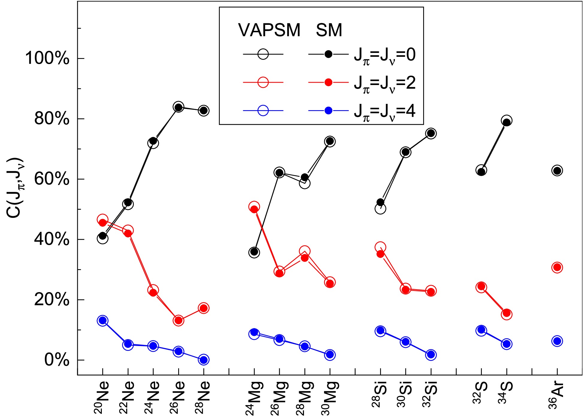
Figure 1. (color online) Calculated
$ C(J_\pi,J_\nu) $ values for the ground states of even-even sd-shell nuclei using the shell model and VAPSM. The USDB interaction is employed.One can readily see that both SM and VAPSM yield very similar
$ C(J_\pi,J_\nu) $ values. This implies that the approximate VAPSM wave functions are quite close to their corresponding exact SM counterparts. This also confirms the validity of the present formulae. Nevertheless, all the calculated$ C(J_\pi=0,J_\nu=0) $ values are less than 1, while the$ C(J_\pi=2,J_\nu=2) $ values are significant. For 20Ne and 24Mg, the$ C(J_\pi=2,J_\nu=2) $ values are even larger than the$ C(J_\pi=0,J_\nu=0) $ values. This indicates that, even in the ground states of even-even nuclei, like nucleons are not fully paired because, in the components with$ J_\pi=J_\nu=2 $ , at least two like nucleons are not coupled to spin zero.The appearance of the
$ J_\pi=J_\nu\neq 0 $ components is clearly due to the neutron-proton interaction present in the adopted Hamiltonian. This can be understood as follows. Let us remove the neutron-proton interaction from the adopted Hamiltonian. Then the Hamiltonian can be written as$ \begin{aligned} H= H^\pi+ H^\nu. \end{aligned} $
(25) This implies that the nuclear system can be separated into two independent subsystems, namely the neutron and proton subsystems. In each subsystem, the ground state is formed with all like nucleons paired, and the corresponding wave function has zero spin and positive parity. The ground state of the total nuclear system is then simply the product of the ground states of these two subsystems. Hence, the ground state for the Hamiltonian of Eq.(26) contains only the
$ J_\pi=J_\nu=0 $ component. Therefore, the neutron-proton interaction leads to admixtures of$ J_\pi=J_\nu\neq 0 $ components in the ground states of even-even nuclei.One can imagine that, as the strength of the neutron-proton interaction increases from zero, the mixing of the
$ J_\pi=J_\nu\neq 0 $ components correspondingly increases. The$ N=Z $ nuclei seem to have the strongest neutron-proton interactions. Indeed, as seen in Fig. 1, for the ground states of 20Ne, 24Mg, 28Si, 32S and 36Ar, the weights of the$ J_\pi=J_\nu=2 $ components are relatively large, and such$ J_\pi=J_\nu=2 $ components are even predominant in 20Ne and 24Mg. One can also see from Fig. 1 that, as the neutron number increases away from$ N=Z $ ,$ C(J_\pi=0,J_\nu=0) $ roughly increases, whereas$ C(J_\pi=2,J_\nu=2) $ roughly decreases. This implies that the neutron-proton interaction becomes weaker as N increases away from$ N=Z $ .For nonzero spin states, the decomposition of the corresponding wave function is more complicated because
$ J_\pi $ and$ J_\nu $ can differ. We performed the same calculations as in Fig. 1, but changed the spin from$ J=0 $ to$ J=2 $ . The result for the yrast$ 2^+ $ state in 24Mg is shown in Fig. 2. Again, the distribution of$ C(J_\pi,J_\nu) $ from VAPSM is very similar to that from the exact SM. The main components for the yrast$ 2^+ $ state in 24Mg are those with$ (J_\pi=0,J_\nu=2) $ ,$ (J_\pi=2,J_\nu=0) $ , and$ (J_\pi=2,J_\nu=2) $ . Similar calculations for the odd-mass nucleus 25Mg and the odd-odd nucleus 26Al were also performed. The results for their ground states are shown in Figs. 3 and 4. In Fig. 3, the ground state of 25Mg is dominated by the$ (J_\pi=0,J_\nu=5/2) $ and$ (J_\pi=2,J_\nu=5/2) $ components. In particular, the latter component arises from the neutron-proton interaction in the USDB Hamiltonian.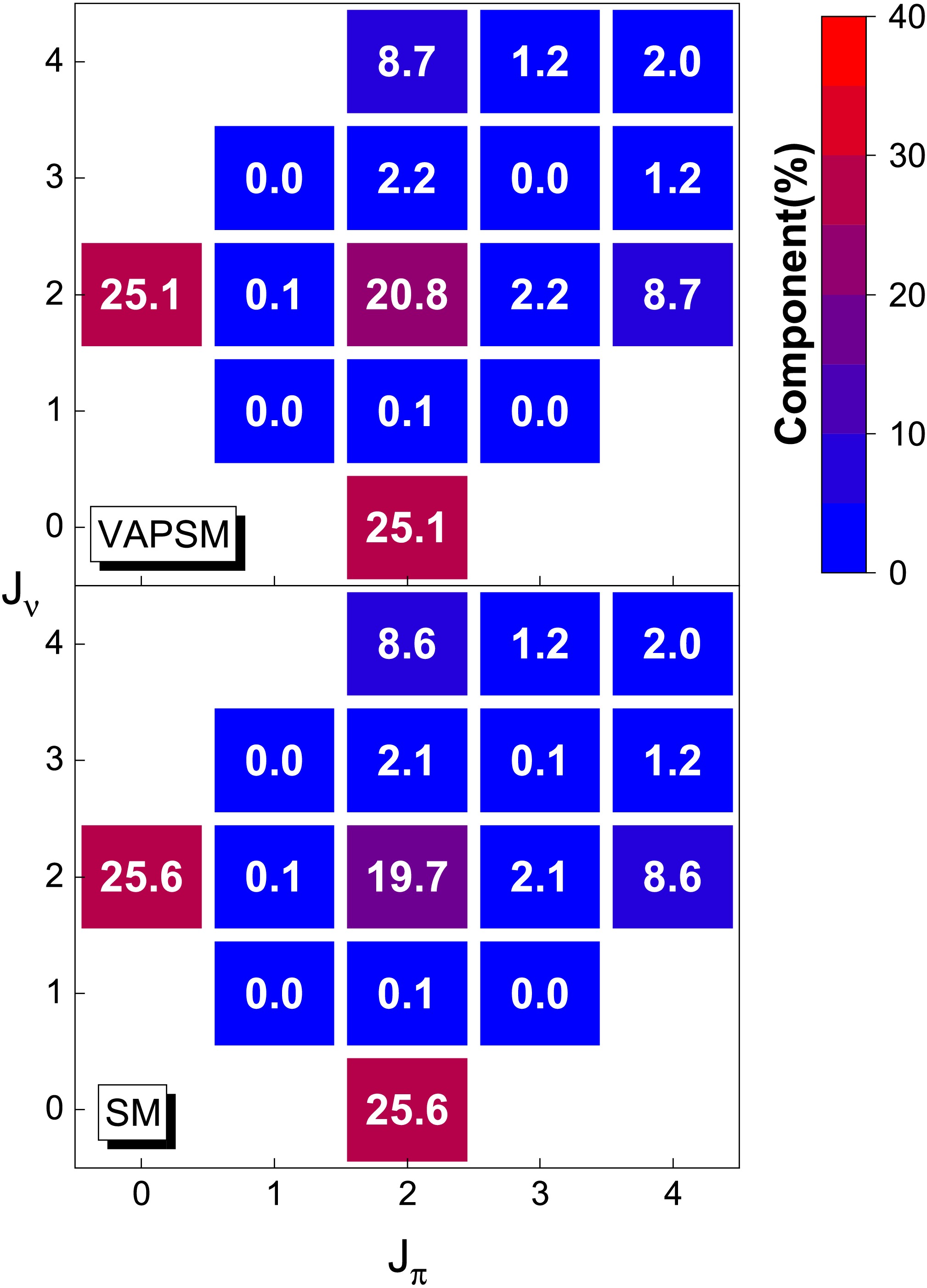
Figure 2. (color online) Distributions of the calculated
$ C(J_\pi,J_\nu) $ values for the yrast$ 2^+ $ state in 24Mg obtained with VAPSM (upper panel) and with the shell model (lower panel). The USDB interaction is employed.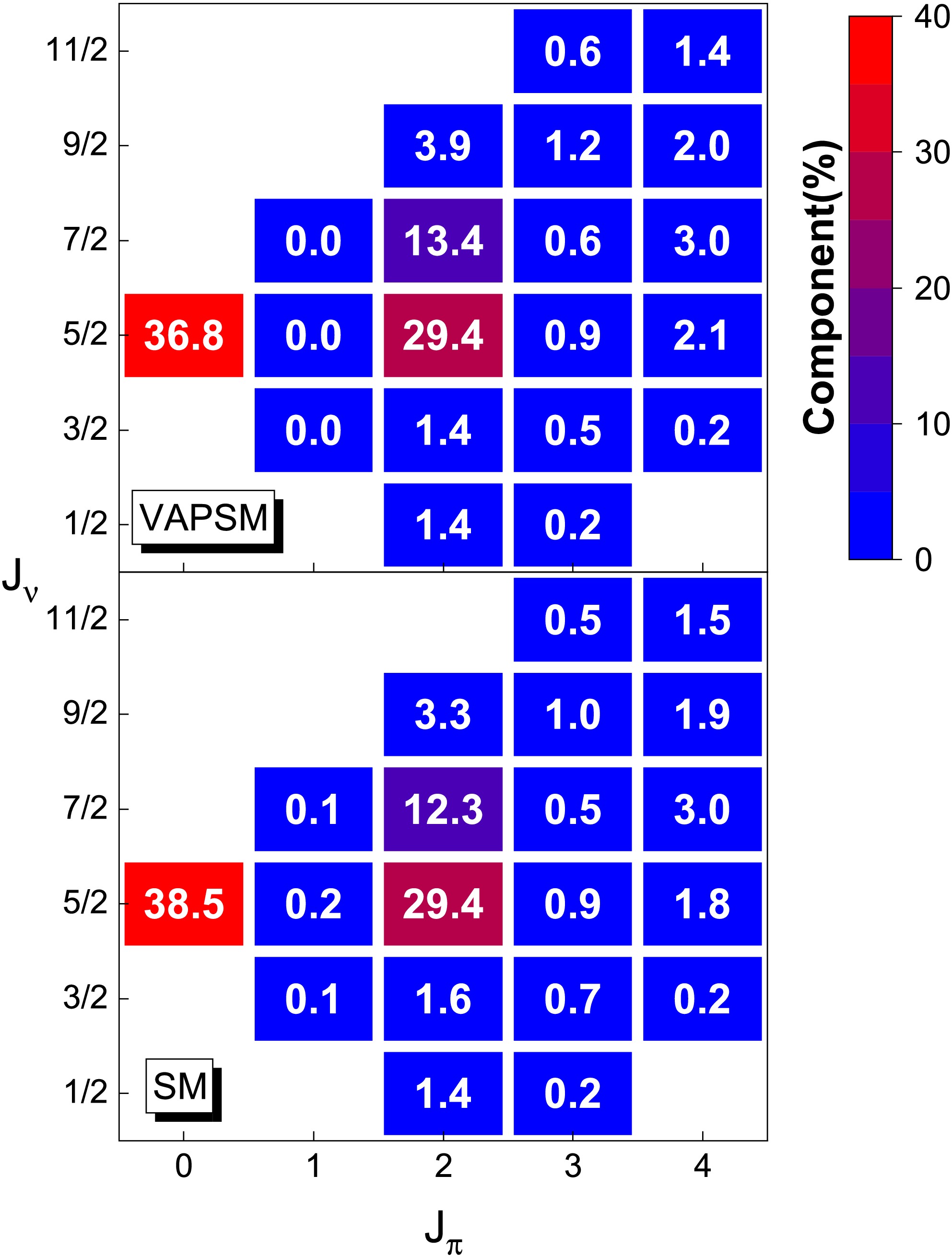
Figure 3. (color online) The same as Fig. 2, but for the
$ 5/2^+ $ ground state of 25Mg.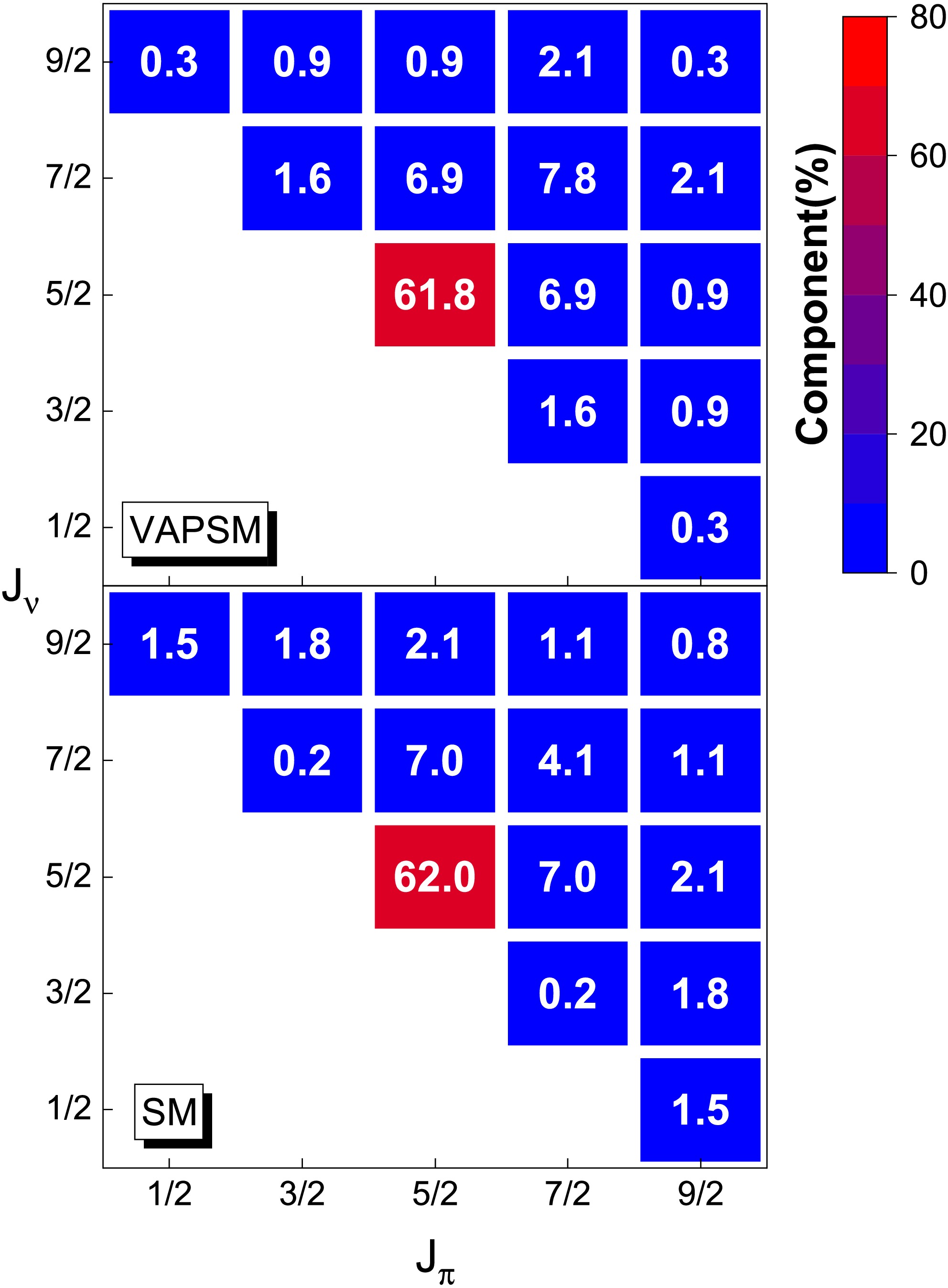
Figure 4. (color online) Same as Fig. 2, but for the
$ 5^+ $ ground state of 26Al.One may observe in Figs. 2 and 3 that when
$ J_\pi $ or$ J_\nu $ is odd, the corresponding$ C(J_\pi,J_\nu) $ becomes very small. This is also indicated in Fig. 1, where those small$ C(J_\pi,J_\nu) $ values are not shown. This behavior may be caused by time-reversal symmetry. If a deformed intrinsic state has time-reversal symmetry, one can prove that the possible angular-momentum projected states with positive parity and$ K=0 $ are those with even J [37]. This is why, in even-even nuclei, the ground-state bands include only states with even J. In the lowest proton (neutron) configuration with an even particle number, all protons (neutrons) governed by the Hamiltonian are likely to form pairs. One can easily understand that such a configuration may have time-reversal symmetry. Therefore, the projected states with$ K_\pi^\pi=0^+ $ ($ K_\nu^\pi=0^+ $ ) can only have even$ J_\pi $ ($ J_\nu $ ). Consequently,$ C(J_\pi,J_\nu) $ should vanish when$ J_\pi $ ($ J_\nu $ ) is odd. A small nonzero value of$ C(J_\pi,J_\nu) $ with odd$ J_\pi $ ($ J_\nu $ ) implies that time-reversal symmetry might be slightly broken.For the ground state in 26Al, the dominant component in Fig. 4 is
$ (J_\pi=5/2,J_\nu=5/2) $ , which indicates that the spins of the neutrons and protons are parallel. One may also consider the possibility that these spins are antiparallel and form a$ 0^+ $ state. Indeed, we calculated the yrast$ 0^+ $ state in 26Al, and the results are shown in Fig. 5. Both the shell-model and VAPSM results show that this$ 0^+ $ state is also dominated by the$ (J_\pi=5/2,J_\nu=5/2) $ component.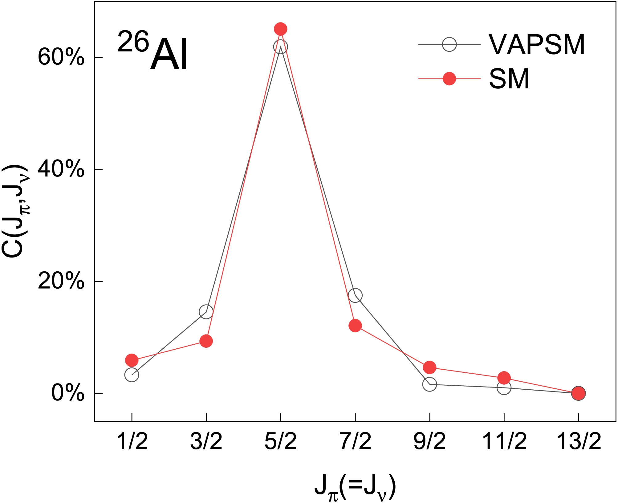
Figure 5. (color online) Distribution of the calculated
$ C(J_\pi,J_\nu) $ values for the yrast$ 0^+ $ state in 26Al from shell-model and VAPSM calculations using the USDB interaction.Based on the above analysis, this decomposition of the angular-momentum projected nuclear wave function is very helpful for studying the structure of the calculated nuclear states. This opens the possibility that such a decomposition can be applied to any heavy, deformed nucleus once its angular-momentum projected wave function is available.
However, in heavy, deformed nuclear regions, intruder orbits with opposite parity are usually included in the model space. In this case, parity projection is adopted, and the VAPSM wave function in Eq. (22) can be written as
$ \begin{aligned} |\Psi^\pi_{JM}(K)\rangle=\sum_{i}f_{i} P^\pi P^J_{MK}|\Phi_i\rangle, \end{aligned} $
(26) where
$ P^\pi=\dfrac{1}{2}(1+\pi \hat{P}) $ is the parity projection operator, with$ \pi=\pm1 $ and$ \hat{P} $ the parity operator. It is straightforward to see that$ \begin{aligned} P^\pi=\sum_{\pi_\pi,\pi_\nu}P^{\pi_\pi}P^{\pi_\nu} \end{aligned} $
(27) where
$ P^{\pi_\pi} $ and$ P^{\pi_\nu} $ are the parity-projection operators for protons and neutrons, respectively. The proton and neutron parities,$ \pi_\pi $ and$ \pi_\nu $ , satisfy$ \pi_\pi\pi_\nu=\pi $ . Consequently, the$ C(J_\pi,J_\nu) $ component is decomposed into two parts, namely,$ \begin{aligned} C(J_\pi,J_\nu)=C(J^+_\pi,J^+_\nu)+C(J^-_\pi,J^-_\nu) \end{aligned} $
(28) for
$ \pi=+1 $ state, or$ \begin{aligned} C(J_\pi,J_\nu)=C(J^+_\pi,J^-_\nu)+C(J^-_\pi,J^+_\nu) \end{aligned} $
(29) for the
$ \pi=-1 $ state.$ J^{\pi_\tau}_\tau $ denotes the spin and parity of the protons ($ \tau=\pi $ ) or neutrons ($ \tau=\nu $ ). Similar to Eq. (23),$ C(J^{\pi_\pi}_\pi,J^{\pi_\nu}_\nu) $ can be calculated by$ \begin{aligned}[b] &C(J^{\pi_\pi}_\pi,J^{\pi_\nu}_\nu)\\=\;&\sum_{K'_{\pi}i'K_{\pi}i}\langle J_{\pi}K'_{\pi}J_{\nu}K-K'_{\pi}|JK\rangle\langle J_{\pi}K_{\pi}J_{\nu}K-K_{\pi}|JK\rangle\\&\times f^*_{i'}f_{i}\langle\Phi^\pi_{i'}| P^{\pi_\pi}P^{J_{\pi}}_{K'_{\pi}K_{\pi}}|\Phi^\pi_i\rangle\langle\Phi^\nu_{i'}| P^{\pi_\nu} P^{J_{\nu}}_{K-K'_{\pi},K-K_{\pi}}|\Phi^\nu_i\rangle. \end{aligned} $
(30) To demonstrate the decomposition in a heavy, deformed nucleus, we calculate the ground-state band with
$ K^\pi=0^+ $ in 166Dy. The adopted model space includes all single-particle orbits between the shell closures of 132Sn and 208Pb, which is usually referred to as the jj56pn model space. In this model space, the dimension of the configuration space for 166Dy reaches$ 1.0\times 10^{17} $ , well beyond the scope of traditional shell-model calculations. The adopted shell-model Hamiltonian is jj56pnb [38], developed for nuclei near 132Sn. Here, we use the wave function of Eq. (27) including only one SD. Using the algorithm in Ref. [28], the states in the rotational band can be obtained simultaneously. The calculated ground-state band energies in 166Dy from VAPSM, together with the corresponding experimental data, are shown in Fig. 6. One can see that, as spin increases, the calculated rotational energy increases faster than the experimental one. This discrepancy indicates that the adopted jj56pnb Hamiltonian might become less effective for 166Dy, since 166Dy lies far from 132Sn. However, with this Hamiltonian, the rotational character of the ground-state band in 166Dy is clearly reproduced. As a preliminary step, we take the wave functions corresponding to the calculated energies in Fig. 6 and decompose them using Eq. (31).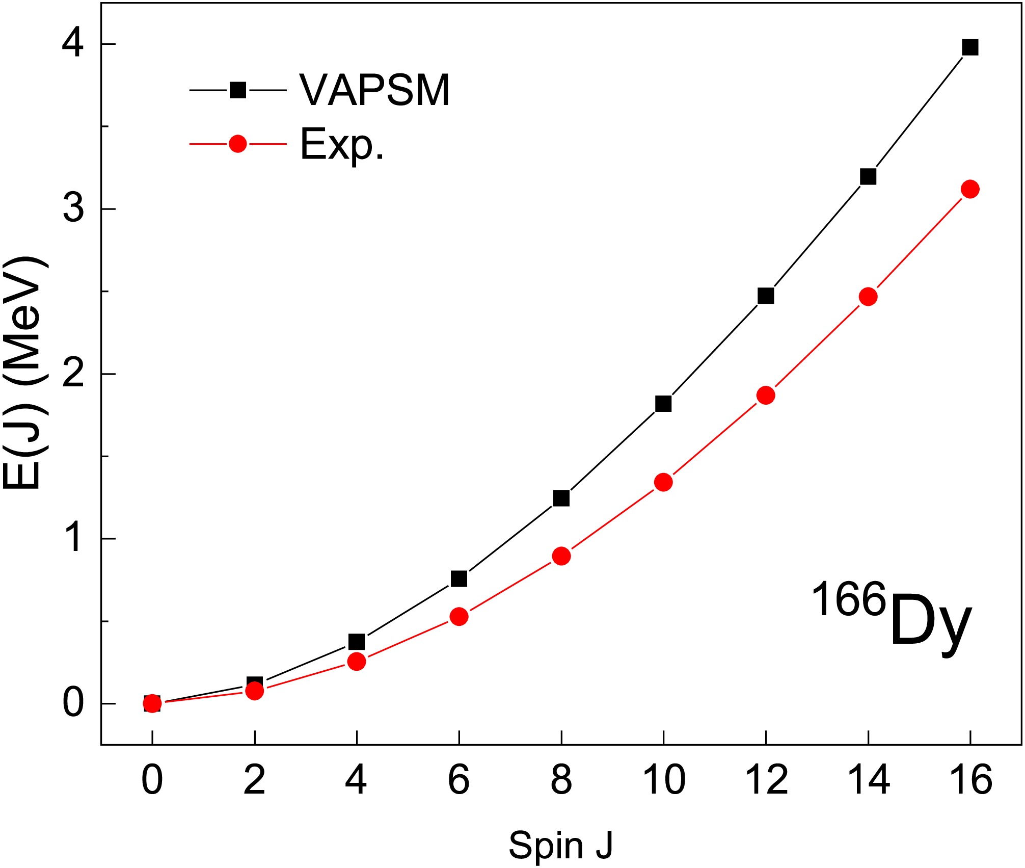
Figure 6. (color online) Calculated ground-state band energies and the corresponding experimental data for 166Dy are presented. The jj56pnb interaction is employed.
The cutoff values for
$ J_\pi $ and$ J_\nu $ are$ J_\pi=J_\nu=20 $ . All the calculated components with$ J_\pi\leq20 $ and$ J_\nu\leq20 $ account for 99.9998%, 99.999%, and 99.94% of the wave functions with$ J^\pi=0^+, 2^+ $ , and$ 10^+ $ , respectively. For the ground state with$ J^\pi=0^+ $ , the calculated$ C(J_\pi,J_\nu) $ ,$ C(J^+_\pi,J^+_\nu) $ , and$ C(J^-_\pi,J^-_\nu) $ values in Eq. (29) are shown in Fig. 7. It is clear that the$ C(J^-_\pi,J^-_\nu) $ values are almost zero. Indeed, the sum of all$ C(J^-_\pi,J^-_\nu) $ values in Fig. 7 is about 0.042%. Unlike Fig. 1, the predominant components in Fig. 7 are those with$ J_\pi=J_\nu=2, 4 $ , and$ 6 $ , each exceeding 15%, whereas$ C(J_\pi=0,J_\nu=0) $ is only about 3.2%. This result is very similar to that for 156Sm with an axial intrinsic state in Ref. [34]. However, here the adopted SD can be arbitrarily deformed. In this$ J=0 $ case, the nonzero$ J_\pi $ and$ J_\nu $ angular momenta must be anti-aligned, as has been extensively discussed in Refs. [34, 39, 40].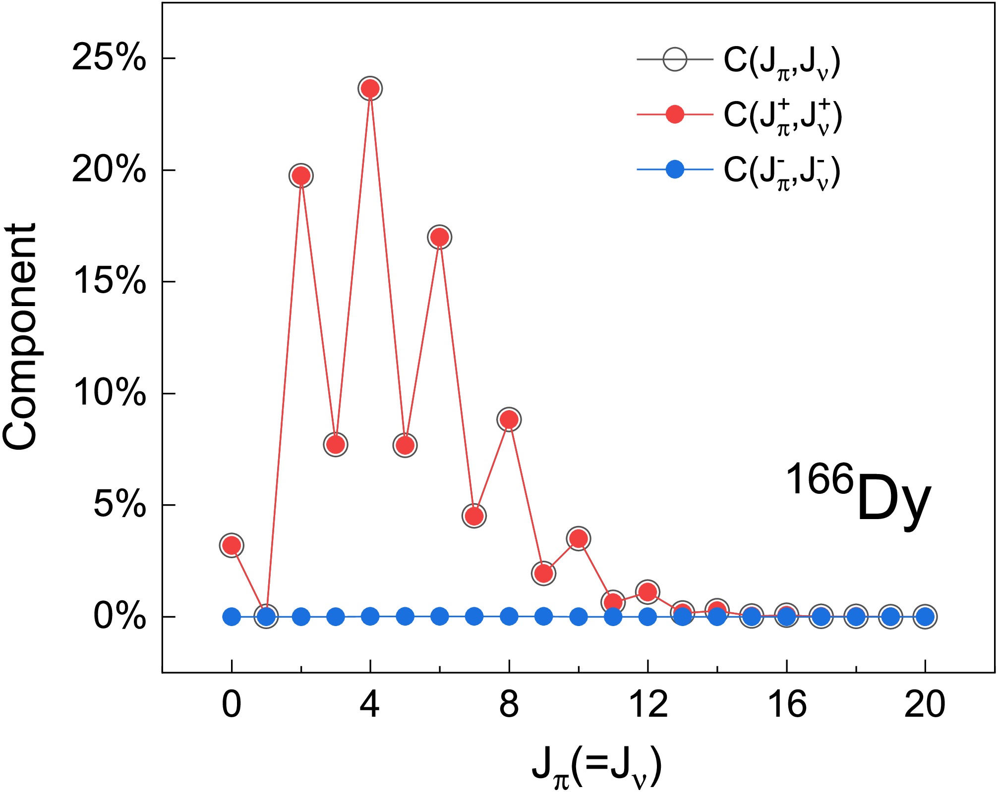
Figure 7. (color online) Distributions of the calculated
$ C(J_\pi,J_\nu) $ ,$ C(J^+_\pi,J^+_\nu) $ , and$ C(J^-_\pi,J^-_\nu) $ values for the VAPSM wave function of the ground$ 0^+ $ state in 166Dy.For other calculated nonzero-spin states, the
$ C(J^-_\pi,J^-_\nu) $ values are likewise very close to zero. For example, at$ J^\pi=2^+ $ and$ 10^+ $ , the sums of the calculated$ C(J^-_\pi,J^-_\nu) $ values are 0.049% and 0.058%, respectively. Thus, we have$ C(J_\pi,J_\nu)\approx C(J^+_\pi,J^+_\nu) $ for the present case of 166Dy. The decompositions of the VAPSM wave functions for$ J^\pi=2^+ $ and$ 10^+ $ are shown in Fig. 8. For$ J^\pi=2^+ $ , the predominant components are those with$ J_\pi $ and/or$ J_\nu $ equal to 4 and 6, whereas the expected$ J_\pi+J_\nu=2 $ components are quite small. For$ J^\pi=10^+ $ , the$ J_\pi+J_\nu=10 $ components predominate, indicating that the proton and neutron deformed ellipsoids rotate in almost the same direction [34, 39, 40].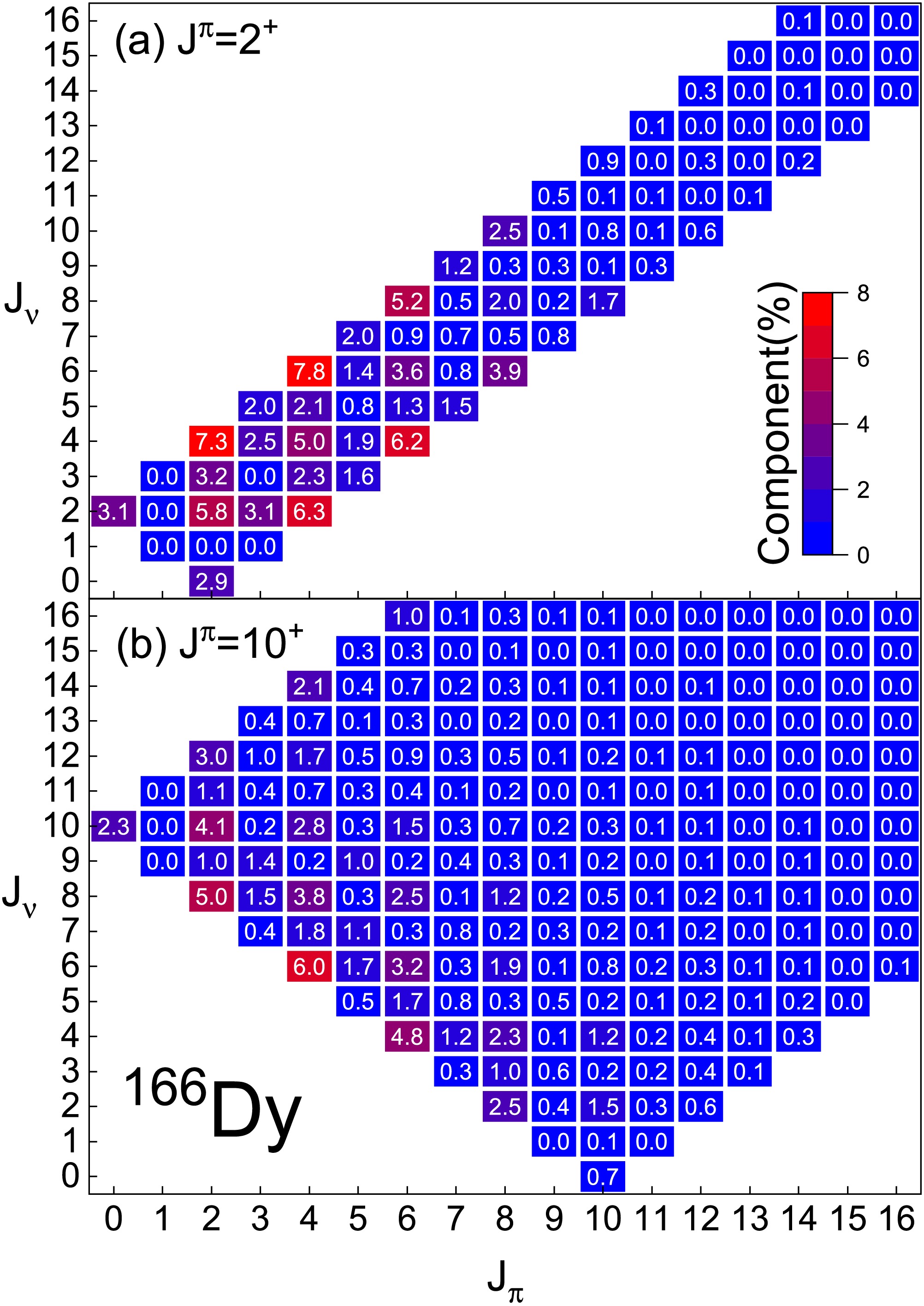
Figure 8. (color online) Distributions of the calculated
$ C(J_\pi,J_\nu) $ values for the VAPSM wave functions associated with the$ 2^+ $ and$ 10^+ $ states in 166Dy. -
According to Eq. (19), the standard projected wave function in Eq. (18) can be expressed in a more general form,
$ \begin{aligned} |\Psi_{JM}\rangle=\sum_{J_{\pi}J_{\nu}K_{\pi}K_{\nu}i}f_{J_{\pi}J_{\nu}K_{\pi}K_{\nu}i} P^{J_{\pi}J_{\nu}}_{JM}(K_{\pi}K_{\nu})|\Phi_i\rangle, \end{aligned} $
(32) where
$ f_{J_{\pi}J_{\nu}K_{\pi}K_{\nu}i}=f_{K i}\langle J_{\pi}K_{\pi}J_{\nu}K_{\nu}|JK\rangle $ . The$ f_{K i} $ coefficients, as well as the SDs$ |\Phi_i\rangle $ , can be obtained by performing VAPSM calculations based on Eq. (18). However, if we treat the$ f_{J_{\pi}J_{\nu}K_{\pi}K_{\nu}i} $ coefficients as free parameters, that is, we recalculate$ f_{J_{\pi}J_{\nu}K_{\pi}K_{\nu}i} $ by diagonalizing the Hamiltonian in the space spanned by the$ P^{J_{\pi}J_{\nu}}_{JM}(K_{\pi}K_{\nu})|\Phi_i\rangle $ basis states, the shell-model approximation within VAPSM may be further improved. For brevity, we rewrite Eq. (32) in a more concise form$ \begin{aligned} |\Psi_{JM}\rangle=\sum_{\alpha i}f_{\alpha i}P_{JM}(\alpha)|\Phi_i\rangle, \end{aligned} $
(32) where α denotes the tuple
$ (J_{\pi}, J_{\nu}, K_{\pi}, K_{\nu}) $ and$ \begin{aligned} P_{JM}(\alpha)\equiv P^{J_{\pi}J_{\nu}}_{JM}(K_{\pi}K_{\nu}). \end{aligned} $
(33) Here we adopt the simplified wave function given in Eq. (22) to perform VAPSM calculations. As in Eq. (32), Eq. (22) can be written as:
$ \begin{aligned} |\Psi_{JM}(K)\rangle=\sum_{\alpha i}f_{\alpha i} P_{JM}(\alpha )|\Phi_i\rangle, \end{aligned} $
(34) where
$ f_{\alpha i}=f_{i}\langle J_{\pi}K_{\pi}J_{\nu}K_{\nu}|JK\rangle $ . However,$ K_{\pi} $ and$ K_{\nu} $ are no longer independent, as they are constrained to satisfy$ K_{\pi}+K_{\nu}=K $ , where K is fixed.To obtain the fully optimized
$ f_{\alpha i} $ coefficients and the corresponding energy E, one should solve the following generalized eigenvalue equation:$ \begin{aligned} \sum_{\alpha' i'}(H_{\alpha i,\alpha' i'}-E N_{\alpha i,\alpha' i'})f_{\alpha' i'}=0 ,\end{aligned} $
(35) where α′ denotes the numbers
$ (J'_{\pi}, J'_{\nu}, K'_{\pi}, K'_{\nu}) $ .$ \begin{aligned} N_{\alpha i,\alpha' i'}=\;&\langle \Phi_i|P^\dagger_{JM}(\alpha)P_{JM}(\alpha')|\Phi_{i'}\rangle\\ =\;&\sum_{M_\pi,M_\nu,M'_\pi,M'_\nu}\langle J_\pi M_\pi J_\nu M_\nu|JM\rangle\langle J_\pi'M_\pi'J_\nu'M_\nu'|JM\rangle\\ &\times\langle\Phi^\pi_i|{P}_{K_\pi M_\pi}^{J_\pi}{P}_{M_\pi'K_\pi'}^{J_\pi'}|\Phi^\pi_{i'}\rangle\langle\Phi^\nu_i|{P}_{K_\nu M_\nu}^{J_\nu}{P}_{M_\nu'K_\nu'}^{J_\nu'}|\Phi^\nu_{i'}\rangle\\ =\;&\langle\Phi^\pi_i|{P}_{K_\pi K_\pi'}^{J_\pi}|\Phi^\pi_{i'}\rangle\langle\Phi^\nu_i|{P}_{K_\nu K_\nu'}^{J_\nu}|\Phi^\nu_{i'}\rangle\delta_{J_\pi J_\pi'}\delta_{J_\nu J_\nu'}, \end{aligned} $
(36) To calculate the matrix element
$ H_{\alpha i,\alpha' i'} $ , the shell-model Hamiltonian is divided into three parts:$ \begin{aligned} H= H^\pi+ H^\nu+ H^{\pi\nu}. \end{aligned} $
(37) In Eq. (38), the like-nucleon part,
$ H^\tau $ (with$ \tau=\pi $ or ν), is given by$ \begin{aligned}[b] H^\tau=\;&\sum_{r_\tau}\epsilon_{r_\tau} \hat N_{r_\tau}+\sum_{{r_\tau}\leq{s_\tau},{t_\tau}\leq{u_\tau},J}\\ &\times\left[\frac{V_{{r_\tau}{s_\tau}{t_\tau}{u_\tau}}^J}{\sqrt{(1+\delta_{r_\tau s_\tau})(1+\delta_{t_\tau u_\tau})}} \sum_M A^{\dagger}_{JM}(r_\tau s_\tau) A_{JM}(t_\tau u_\tau)\right]. \end{aligned} $
(38) Here,
$ \hat N_{r_\tau} $ is the operator that measures the number of nucleons in the$ {r_\tau} $ subshell with quantum numbers ($ n_{r_\tau} $ ,$ l_{r_\tau} $ ,$ j_{r_\tau} $ ), i.e.,$ \begin{aligned} \hat N_{r_\tau}=\sum_{m_{r_\tau}} c^\dagger_{r_\tau m_{r_\tau}} c_{r_\tau m_{r_\tau}}, \end{aligned} $
(39) where
$ c^\dagger_{r_\tau m_{r_\tau}} $ ($ c_{r_\tau m_{r_\tau}} $ ) is the spherical harmonic-oscillator single-particle creation (annihilation) operator with quantum numbers ($ n_{r_\tau} $ ,$ l_{r_\tau} $ ,$ j_{r_\tau} $ ,$ m_{r_\tau} $ ).$ A^{\dagger}_{JM}(r_\tau s_\tau) $ is the nucleon-pair creation operator defined as:$ \begin{aligned} A^{\dagger}_{JM}(r_\tau s_\tau)=\sum_{m_{r_\tau}m_{s_\tau}}\langle j_{r_\tau}m_{r_\tau}j_{s_\tau}m_{s_\tau}|JM\rangle c^\dagger_{r_\tau m_{r_\tau}} c^\dagger_{s_\tau m_{s_\tau}}\\ \end{aligned} $
(40) and
$ \begin{aligned} A_{JM}(t_\tau u_\tau)=\sum_{m_{t_\tau}m_{u_\tau}}\langle j_{t_\tau}m_{t_\tau}j_{u_\tau}m_{u_\tau}|JM\rangle c_{u_\tau m_{u_\tau}} c_{t_\tau m_{t_\tau}}.\\ \end{aligned} $
(41) The neutron-proton interaction term,
$ H^{\pi\nu} $ , can be written as:$ \begin{aligned} H^{\pi\nu}=\sum_{r_{\pi}s_{\nu}t_{\pi}u_{\nu},J}V_{r_{\pi}s_{\nu}t_{\pi}u_{\nu}}^{J}\sum_{M}A_{JM}^{\dagger}(r_{\pi}s_{\nu})A_{JM}(t_{\pi}u_{\nu}),\\ \end{aligned} $
(42) where
$ \begin{aligned} A^{\dagger}_{JM}(r_\pi s_\nu)=\sum_{m_{r_\pi}m_{s_\nu}}\langle j_{r_\pi}m_{r_\pi}j_{s_\nu}m_{s_\nu}|JM\rangle c^\dagger_{r_\pi m_{r_\pi}} c^\dagger_{s_\nu m_{s_\nu}}\\ \end{aligned} $
(43) and
$ \begin{aligned} A_{JM}(t_\pi u_\nu)=\sum_{m_{t_\pi}m_{u_\nu}}\langle j_{t_\pi}m_{t_\pi}j_{u_\nu}m_{u_\nu}|JM\rangle c_{u_\nu m_{u_\nu}} c_{t_\pi m_{t_\pi}}.\\ \end{aligned} $
(44) Accordingly, the matrix element
$ H_{\alpha i,\alpha' i'} $ can be decomposed into three parts,$ \begin{aligned}[b] H_{\alpha i,\alpha' i'}&=\langle \Phi_i|P^\dagger_{JM}(\alpha) H P_{JM}(\alpha')|\Phi_{i'}\rangle\\ &=H^\pi_{\alpha i,\alpha' i'}+H^\nu{}_{\alpha i,\alpha' i'}+H^{\pi\nu}_{\alpha i,\alpha' i'}, \end{aligned} $
(45) where
$ \begin{aligned} H^\pi_{\alpha i,\alpha' i'}&=\langle \Phi_i|P^\dagger_{JM}(\alpha) H^\pi P_{JM}(\alpha')|\Phi_{i'}\rangle\\ &=\langle\Phi^\pi_i|{H}^\pi{P}_{K_\pi K_\pi'}^{J_\pi}|\Phi^\pi_{i'}\rangle\langle\Phi^\nu_i|{P}_{K_\nu K_\nu'}^{J_\nu}|\Phi^\nu_{i'}\rangle\delta_{J_\pi J_\pi'}\delta_{J_\nu J_\nu'}, \end{aligned} $
(46) $ \begin{aligned}[b] H^\nu_{\alpha i,\alpha' i'}&=\langle \Phi_i|P^\dagger_{JM}(\alpha) H^\nu P_{JM}(\alpha')|\Phi_{i'}\rangle\\ &=\langle\Phi^\pi_i|{P}_{K_\pi K_\pi'}^{J_\pi}|\Phi^\pi_{i'}\rangle\langle\Phi^\nu_i|{H}^\nu{P}_{K_\nu K_\nu'}^{J_\nu}|\Phi^\nu_{i'}\rangle\delta_{J_\pi J_\pi'}\delta_{J_\nu J_\nu'} \end{aligned} $
(47) and
$ H^{\pi\nu}_{\alpha i,\alpha' i'}=\langle \Phi_i|P^\dagger_{JM}(\alpha) H^{\pi\nu} P_{JM}(\alpha')|\Phi_{i'}\rangle. $
(48) To evaluate
$ H^{\pi\nu}_{\alpha i,\alpha' i'} $ ,$ H^{\pi\nu} $ needs to be transformed from the particle-particle form into the particle-hole form; namely,$ \begin{aligned}[b] H^{\pi\nu}=&\sum_{r_{\pi}s_{\nu}t_{\pi}u_{\nu},J}V_{r_{\pi}s_{\nu}t_{\pi}u_{\nu}}^{J}\sum_{M}A_{JM}^{\dagger}(r_{\pi}s_{\nu})A_{JM}(t_{\pi}u_{\nu}),\\ =&\sum_{r_{\pi}s_{\nu}t_{\pi}u_{\nu},\lambda}\omega_{r_{\pi}t_{\pi}s_{\nu}u_{\nu}}^{\lambda}\sum_{\mu}(-1)^{\lambda-\mu}S_{\lambda\mu}(r_{\pi}t_{\pi})S_{\lambda-\mu}(s_{\nu}u_{\nu}),\\ =&\sum_{r_{\pi}s_{\nu}t_{\pi}u_{\nu},\lambda}\omega_{r_{\pi}t_{\pi}s_{\nu}u_{\nu}}^{\lambda}(-1)^{\lambda}S_{\lambda}(r_{\pi}t_{\pi})\cdot S_{\lambda}(s_{\nu}u_{\nu}), \end{aligned} $
(49) where
$ \begin{aligned}[b] \begin{split} \omega_{r_{\pi}t_{\pi}s_{\nu}u_{\nu}}^{\lambda}=&\sum_{J}(-1)^{j_{s_{\nu}}+j_{t_{\pi}}-\lambda-J}(2J+1)\\ &\times\begin{Bmatrix} j_{r_{\pi}} & j_{s_{\nu}} & J\\ j_{u_{\nu}} & j_{t_{\pi}} & \lambda \end{Bmatrix}V_{r_{\pi}s_{\nu}t_{\pi}u_{\nu}}^{J}, \end{split} \end{aligned} $
(50) $ \begin{aligned}[b] V_{r_{\pi}s_{\nu}t_{\pi}u_{\nu}}^{J}=&\sum_{\lambda}(-1)^{j_{s_{\nu}}+j_{t_{\pi}}-\lambda-J}(2\lambda+1)\\ &\times \begin{Bmatrix} j_{r_{\pi}} & j_{s_{\nu}} & J\\ j_{u_{\nu}} & j_{t_{\pi}} & \lambda \end{Bmatrix}\omega_{r_{\pi}t_{\pi}s_{\nu}u_{\nu}}^{\lambda}. \end{aligned} $
(51) $ S_{\lambda\mu}(r_\tau t_\tau) $ is a spherical tensor operator defined as follows:$ S_{\lambda\mu}(r_\tau t_\tau )=\sum_{m_{r_\tau}m_{t_\tau}}\langle j_{r_\tau}m_{r_\tau}j_{t_\tau}m_{t_\tau}|\lambda\mu\rangle c^\dagger_{r_\tau m_{r_\tau}}{\tilde{c}}_{t_\tau m_{t_\tau}}, $
(52) where
$ {\tilde{c}}_{t_\tau m_{t_\tau}}=(-1)^{j_{t_\tau}+m_{t_\tau}}{c}_{t_\tau, -m_{t_\tau}} $ . Inserting Eq. (50) into Eq. (49), we obtain$ \begin{aligned}[b] H^{\pi\nu}_{\alpha i,\alpha' i'} =\;&\sum_{r_{\pi}s_{\nu}t_{\pi}u_{\nu},\lambda}\omega_{r_{\pi}t_{\pi}s_{\nu}u_{\nu}}^{\lambda}(-1)^{\lambda}\\ &\times\langle \Phi_i|P^\dagger_{JM}(\alpha)S_{\lambda}(r_{\pi}t_{\pi})\cdot S_{\lambda}(s_{\nu}u_{\nu}) P_{JM}(\alpha')|\Phi_{i'}\rangle\\ =\;&\sum_{r_{\pi}s_{\nu}t_{\pi}u_{\nu},\lambda}\omega_{r_{\pi}t_{\pi}s_{\nu}u_{\nu}}^{\lambda}(-1)^{\lambda}(-1)^{J_{\pi}'+J_{\nu}+J}\\ &\times\begin{Bmatrix} J_{\pi} & J_{\nu} & J\\ J_{\nu}' & J_{\pi}' &\lambda \end{Bmatrix}\langle \psi_{J_{\pi}}(K_{\pi} i)||S_{\lambda}(r_{\pi}t_{\pi})||\psi_{{J'_\pi}}(K'_{\pi} i')\rangle\\ &\times\langle \psi_{J_{\nu}}(K_{\nu}i)||S_{\lambda}(s_{\nu}u_{\nu})||\psi_{{J'_\nu}}(K'_{\nu}i')\rangle, \end{aligned} $
(53) where, we define
$ \begin{aligned} | \psi_{J_\tau M_\tau}(K_\tau i)\rangle=P^{J_\tau}_{M_\tau K_\tau}|\Phi^\tau_i\rangle \end{aligned} $
(54) and the reduced matrix element
$ \langle jm|T_{\lambda\mu}|j'm'\rangle =\frac1{\sqrt{2j+1}}(-1)^{2\lambda}\times \langle j'm'\lambda\mu|jm\rangle\langle j||T_\lambda||j'\rangle. $
(55) The reduced matrix element in Eq. (54) can then be expressed as
$ \begin{aligned}[b] &\langle \psi_{J_{\tau}}(K_{\tau} i)||S_{\lambda}(r_{\tau}t_{\tau})||\psi_{{J'_\tau}}(K'_{\tau} i')\rangle\\ =&\sqrt{2J_\tau+1}\sum_{\mu}\langle J'_\tau K_\tau-\mu\lambda\mu|J_\tau K_\tau\rangle\\ &\times\langle\Phi^\tau_i|S_{\lambda\mu}(r_\tau t_\tau){P}_{K_\tau-\mu,K'_\tau}^{J'_\tau}|\Phi^\tau_{i'}\rangle. \end{aligned} $
(56) The projected matrix elements in Eqs. (47), (48), and (57) can be readily evaluated within the present VAPSM framework. This, in turn, provides the matrix elements in Eq. (36), allowing the generalized eigenvalue equation to be solved.
To demonstrate the improvement afforded by the new projected wave function, we first perform VAPSM calculations for the ground states in several sd-shell nuclei. For simplicity, we adopt only a single SD to construct the VAPSM wave function in Eq.(22). After the VAPSM calculation, the minimized energy and the corresponding optimized VAPSM wave function are obtained. The energy differences between these VAPSM energies and the exact shell-model ones are shown in Fig. 9. These differences are on the order of a few hundred keV, which may appear large in the figure but are actually negligible compared with the absolute energies [26, 41]. The quality of the shell-model approximation can also be seen from Figs.1, 2, 3, 4, and 5, which indicate that the VAPSM wave functions with one SD are very close to the exact shell-model ones. Of course, these energy differences can be reduced to sufficiently small values by adding more SDs to the VAPSM wave functions. However, here we do not add more SDs. Instead, we investigate whether such energy differences can be reduced by adopting the aforementioned coupled projected basis.
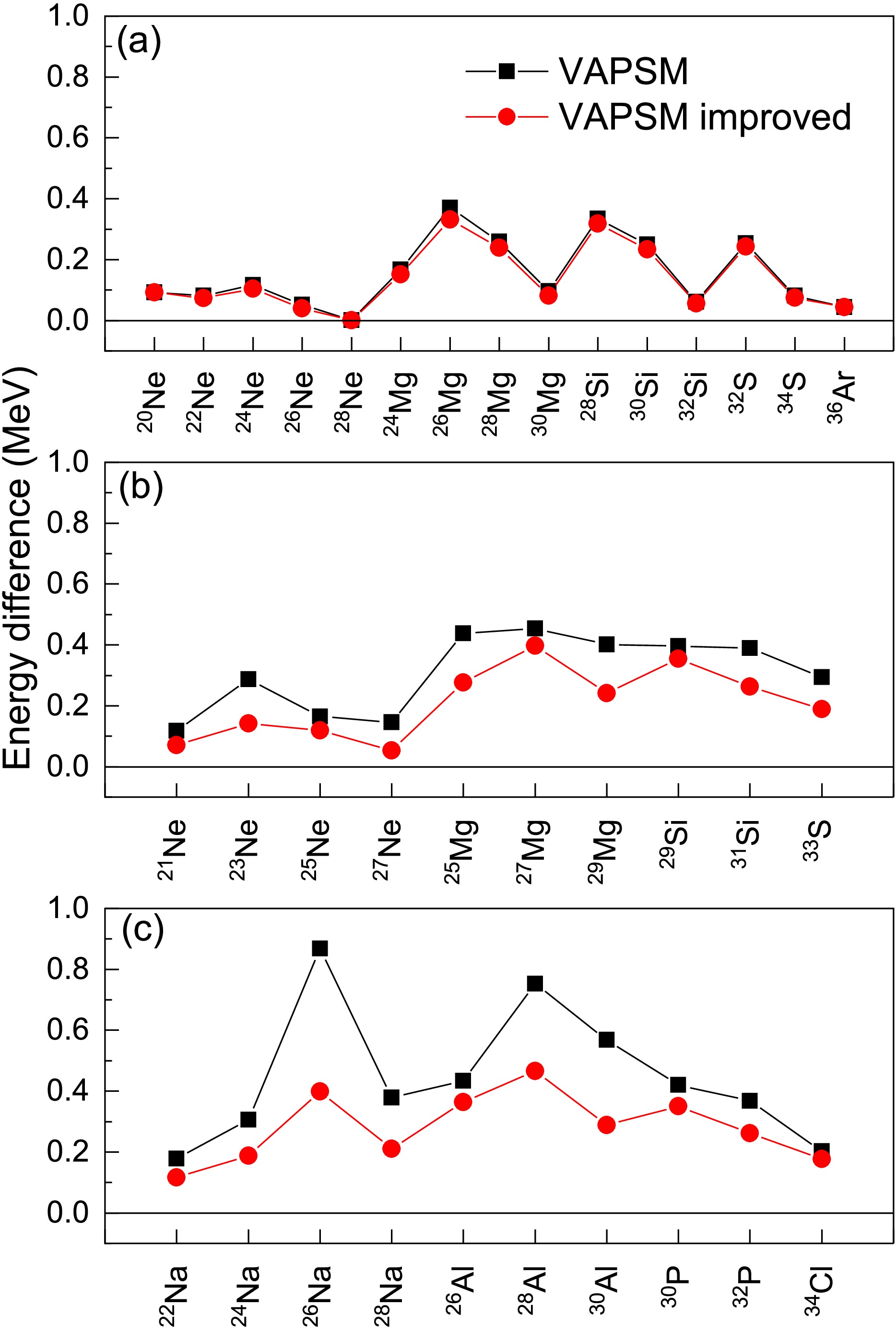
Figure 9. (color online) Calculated energy differences between VAPSM and exact SM ground-state energies for (a) even-even, (b) odd-mass, and (c) odd-odd sd-shell nuclei. The black squares show results for the optimized VAPSM wave function given by Eq. (1). The red dots show results obtained by replacing the optimized form in Eq. (1) with the generalized form in Eq. (35). The USDB interaction is employed.
As a preliminary calculation, we simply use the same SD as in the optimized VAPSM wave function to construct Eq. (35). The coefficients
$ f_{\alpha i} $ and the corresponding energy are obtained by solving Eq. (36). The energy differences between the energies with the new wave functions and the exact shell-model ones are also shown in Fig. 9. For the ground states in even-even nuclei, the improvements with the new wave functions are not significant, indicating that the relative scissors motion between the neutron system and the proton system can be neglected in these calculated states. However, for odd-mass and odd-odd nuclei, the energies with the new wave functions are considerably lowered. This indicates that the coupled projected basis is indeed capable of improving the VAPSM wave function, although that improvement is not complete because the adopted SD is simply taken from the original VAPSM calculation. A full VAPSM calculation with the coupled projected basis would directly vary the wave function in Eq. (35) by simultaneously changing the$ |\Phi_i\rangle $ SDs and the$ f_{\alpha i} $ coefficients. This will be done in the near future. -
According to Eq. (19), the standard projected wave function in Eq. (18) can be expressed in a more general form,
$ \begin{aligned} |\Psi_{JM}\rangle=\sum_{J_{\pi}J_{\nu}K_{\pi}K_{\nu}i}f_{J_{\pi}J_{\nu}K_{\pi}K_{\nu}i} P^{J_{\pi}J_{\nu}}_{JM}(K_{\pi}K_{\nu})|\Phi_i\rangle, \end{aligned} $
(32) where
$ f_{J_{\pi}J_{\nu}K_{\pi}K_{\nu}i}=f_{K i}\langle J_{\pi}K_{\pi}J_{\nu}K_{\nu}|JK\rangle $ . The$ f_{K i} $ coefficients, as well as the SDs$ |\Phi_i\rangle $ , can be obtained by performing VAPSM calculations based on Eq. (18). However, if we treat the$ f_{J_{\pi}J_{\nu}K_{\pi}K_{\nu}i} $ coefficients as free parameters, that is, we recalculate$ f_{J_{\pi}J_{\nu}K_{\pi}K_{\nu}i} $ by diagonalizing the Hamiltonian in the space spanned by the$ P^{J_{\pi}J_{\nu}}_{JM}(K_{\pi}K_{\nu})|\Phi_i\rangle $ basis states, the shell-model approximation within VAPSM may be further improved. For brevity, we rewrite Eq. (32) in a more concise form$ \begin{aligned} |\Psi_{JM}\rangle=\sum_{\alpha i}f_{\alpha i}P_{JM}(\alpha)|\Phi_i\rangle, \end{aligned} $
(32) where α denotes the tuple
$ (J_{\pi}, J_{\nu}, K_{\pi}, K_{\nu}) $ and$ \begin{aligned} P_{JM}(\alpha)\equiv P^{J_{\pi}J_{\nu}}_{JM}(K_{\pi}K_{\nu}). \end{aligned} $
(33) Here we adopt the simplified wave function given in Eq. (22) to perform VAPSM calculations. As in Eq. (32), Eq. (22) can be written as:
$ \begin{aligned} |\Psi_{JM}(K)\rangle=\sum_{\alpha i}f_{\alpha i} P_{JM}(\alpha )|\Phi_i\rangle, \end{aligned} $
(34) where
$ f_{\alpha i}=f_{i}\langle J_{\pi}K_{\pi}J_{\nu}K_{\nu}|JK\rangle $ . However,$ K_{\pi} $ and$ K_{\nu} $ are no longer independent, as they are constrained to satisfy$ K_{\pi}+K_{\nu}=K $ , where K is fixed.To obtain the fully optimized
$ f_{\alpha i} $ coefficients and the corresponding energy E, one should solve the following generalized eigenvalue equation:$ \begin{aligned} \sum_{\alpha' i'}(H_{\alpha i,\alpha' i'}-E N_{\alpha i,\alpha' i'})f_{\alpha' i'}=0 ,\end{aligned} $
(35) where α′ denotes the numbers
$ (J'_{\pi}, J'_{\nu}, K'_{\pi}, K'_{\nu}) $ .$ \begin{aligned} N_{\alpha i,\alpha' i'}=\;&\langle \Phi_i|P^\dagger_{JM}(\alpha)P_{JM}(\alpha')|\Phi_{i'}\rangle\\ =\;&\sum_{M_\pi,M_\nu,M'_\pi,M'_\nu}\langle J_\pi M_\pi J_\nu M_\nu|JM\rangle\langle J_\pi'M_\pi'J_\nu'M_\nu'|JM\rangle\\ &\times\langle\Phi^\pi_i|{P}_{K_\pi M_\pi}^{J_\pi}{P}_{M_\pi'K_\pi'}^{J_\pi'}|\Phi^\pi_{i'}\rangle\langle\Phi^\nu_i|{P}_{K_\nu M_\nu}^{J_\nu}{P}_{M_\nu'K_\nu'}^{J_\nu'}|\Phi^\nu_{i'}\rangle\\ =\;&\langle\Phi^\pi_i|{P}_{K_\pi K_\pi'}^{J_\pi}|\Phi^\pi_{i'}\rangle\langle\Phi^\nu_i|{P}_{K_\nu K_\nu'}^{J_\nu}|\Phi^\nu_{i'}\rangle\delta_{J_\pi J_\pi'}\delta_{J_\nu J_\nu'}, \end{aligned} $
(36) To calculate the matrix element
$ H_{\alpha i,\alpha' i'} $ , the shell-model Hamiltonian is divided into three parts:$ \begin{aligned} H= H^\pi+ H^\nu+ H^{\pi\nu}. \end{aligned} $
(37) In Eq. (38), the like-nucleon part,
$ H^\tau $ (with$ \tau=\pi $ or ν), is given by$ \begin{aligned}[b] H^\tau=\;&\sum_{r_\tau}\epsilon_{r_\tau} \hat N_{r_\tau}+\sum_{{r_\tau}\leq{s_\tau},{t_\tau}\leq{u_\tau},J}\\ &\times\left[\frac{V_{{r_\tau}{s_\tau}{t_\tau}{u_\tau}}^J}{\sqrt{(1+\delta_{r_\tau s_\tau})(1+\delta_{t_\tau u_\tau})}} \sum_M A^{\dagger}_{JM}(r_\tau s_\tau) A_{JM}(t_\tau u_\tau)\right]. \end{aligned} $
(38) Here,
$ \hat N_{r_\tau} $ is the operator that measures the number of nucleons in the$ {r_\tau} $ subshell with quantum numbers ($ n_{r_\tau} $ ,$ l_{r_\tau} $ ,$ j_{r_\tau} $ ), i.e.,$ \begin{aligned} \hat N_{r_\tau}=\sum_{m_{r_\tau}} c^\dagger_{r_\tau m_{r_\tau}} c_{r_\tau m_{r_\tau}}, \end{aligned} $
(39) where
$ c^\dagger_{r_\tau m_{r_\tau}} $ ($ c_{r_\tau m_{r_\tau}} $ ) is the spherical harmonic-oscillator single-particle creation (annihilation) operator with quantum numbers ($ n_{r_\tau} $ ,$ l_{r_\tau} $ ,$ j_{r_\tau} $ ,$ m_{r_\tau} $ ).$ A^{\dagger}_{JM}(r_\tau s_\tau) $ is the nucleon-pair creation operator defined as:$ \begin{aligned} A^{\dagger}_{JM}(r_\tau s_\tau)=\sum_{m_{r_\tau}m_{s_\tau}}\langle j_{r_\tau}m_{r_\tau}j_{s_\tau}m_{s_\tau}|JM\rangle c^\dagger_{r_\tau m_{r_\tau}} c^\dagger_{s_\tau m_{s_\tau}}\\ \end{aligned} $
(40) and
$ \begin{aligned} A_{JM}(t_\tau u_\tau)=\sum_{m_{t_\tau}m_{u_\tau}}\langle j_{t_\tau}m_{t_\tau}j_{u_\tau}m_{u_\tau}|JM\rangle c_{u_\tau m_{u_\tau}} c_{t_\tau m_{t_\tau}}.\\ \end{aligned} $
(41) The neutron-proton interaction term,
$ H^{\pi\nu} $ , can be written as:$ \begin{aligned} H^{\pi\nu}=\sum_{r_{\pi}s_{\nu}t_{\pi}u_{\nu},J}V_{r_{\pi}s_{\nu}t_{\pi}u_{\nu}}^{J}\sum_{M}A_{JM}^{\dagger}(r_{\pi}s_{\nu})A_{JM}(t_{\pi}u_{\nu}),\\ \end{aligned} $
(42) where
$ \begin{aligned} A^{\dagger}_{JM}(r_\pi s_\nu)=\sum_{m_{r_\pi}m_{s_\nu}}\langle j_{r_\pi}m_{r_\pi}j_{s_\nu}m_{s_\nu}|JM\rangle c^\dagger_{r_\pi m_{r_\pi}} c^\dagger_{s_\nu m_{s_\nu}}\\ \end{aligned} $
(43) and
$ \begin{aligned} A_{JM}(t_\pi u_\nu)=\sum_{m_{t_\pi}m_{u_\nu}}\langle j_{t_\pi}m_{t_\pi}j_{u_\nu}m_{u_\nu}|JM\rangle c_{u_\nu m_{u_\nu}} c_{t_\pi m_{t_\pi}}.\\ \end{aligned} $
(44) Accordingly, the matrix element
$ H_{\alpha i,\alpha' i'} $ can be decomposed into three parts,$ \begin{aligned}[b] H_{\alpha i,\alpha' i'}&=\langle \Phi_i|P^\dagger_{JM}(\alpha) H P_{JM}(\alpha')|\Phi_{i'}\rangle\\ &=H^\pi_{\alpha i,\alpha' i'}+H^\nu{}_{\alpha i,\alpha' i'}+H^{\pi\nu}_{\alpha i,\alpha' i'}, \end{aligned} $
(45) where
$ \begin{aligned} H^\pi_{\alpha i,\alpha' i'}&=\langle \Phi_i|P^\dagger_{JM}(\alpha) H^\pi P_{JM}(\alpha')|\Phi_{i'}\rangle\\ &=\langle\Phi^\pi_i|{H}^\pi{P}_{K_\pi K_\pi'}^{J_\pi}|\Phi^\pi_{i'}\rangle\langle\Phi^\nu_i|{P}_{K_\nu K_\nu'}^{J_\nu}|\Phi^\nu_{i'}\rangle\delta_{J_\pi J_\pi'}\delta_{J_\nu J_\nu'}, \end{aligned} $
(46) $ \begin{aligned}[b] H^\nu_{\alpha i,\alpha' i'}&=\langle \Phi_i|P^\dagger_{JM}(\alpha) H^\nu P_{JM}(\alpha')|\Phi_{i'}\rangle\\ &=\langle\Phi^\pi_i|{P}_{K_\pi K_\pi'}^{J_\pi}|\Phi^\pi_{i'}\rangle\langle\Phi^\nu_i|{H}^\nu{P}_{K_\nu K_\nu'}^{J_\nu}|\Phi^\nu_{i'}\rangle\delta_{J_\pi J_\pi'}\delta_{J_\nu J_\nu'} \end{aligned} $
(47) and
$ H^{\pi\nu}_{\alpha i,\alpha' i'}=\langle \Phi_i|P^\dagger_{JM}(\alpha) H^{\pi\nu} P_{JM}(\alpha')|\Phi_{i'}\rangle. $
(48) To evaluate
$ H^{\pi\nu}_{\alpha i,\alpha' i'} $ ,$ H^{\pi\nu} $ needs to be transformed from the particle-particle form into the particle-hole form; namely,$ \begin{aligned}[b] H^{\pi\nu}=&\sum_{r_{\pi}s_{\nu}t_{\pi}u_{\nu},J}V_{r_{\pi}s_{\nu}t_{\pi}u_{\nu}}^{J}\sum_{M}A_{JM}^{\dagger}(r_{\pi}s_{\nu})A_{JM}(t_{\pi}u_{\nu}),\\ =&\sum_{r_{\pi}s_{\nu}t_{\pi}u_{\nu},\lambda}\omega_{r_{\pi}t_{\pi}s_{\nu}u_{\nu}}^{\lambda}\sum_{\mu}(-1)^{\lambda-\mu}S_{\lambda\mu}(r_{\pi}t_{\pi})S_{\lambda-\mu}(s_{\nu}u_{\nu}),\\ =&\sum_{r_{\pi}s_{\nu}t_{\pi}u_{\nu},\lambda}\omega_{r_{\pi}t_{\pi}s_{\nu}u_{\nu}}^{\lambda}(-1)^{\lambda}S_{\lambda}(r_{\pi}t_{\pi})\cdot S_{\lambda}(s_{\nu}u_{\nu}), \end{aligned} $
(49) where
$ \begin{aligned}[b] \begin{split} \omega_{r_{\pi}t_{\pi}s_{\nu}u_{\nu}}^{\lambda}=&\sum_{J}(-1)^{j_{s_{\nu}}+j_{t_{\pi}}-\lambda-J}(2J+1)\\ &\times\begin{Bmatrix} j_{r_{\pi}} & j_{s_{\nu}} & J\\ j_{u_{\nu}} & j_{t_{\pi}} & \lambda \end{Bmatrix}V_{r_{\pi}s_{\nu}t_{\pi}u_{\nu}}^{J}, \end{split} \end{aligned} $
(50) $ \begin{aligned}[b] V_{r_{\pi}s_{\nu}t_{\pi}u_{\nu}}^{J}=&\sum_{\lambda}(-1)^{j_{s_{\nu}}+j_{t_{\pi}}-\lambda-J}(2\lambda+1)\\ &\times \begin{Bmatrix} j_{r_{\pi}} & j_{s_{\nu}} & J\\ j_{u_{\nu}} & j_{t_{\pi}} & \lambda \end{Bmatrix}\omega_{r_{\pi}t_{\pi}s_{\nu}u_{\nu}}^{\lambda}. \end{aligned} $
(51) $ S_{\lambda\mu}(r_\tau t_\tau) $ is a spherical tensor operator defined as follows:$ S_{\lambda\mu}(r_\tau t_\tau )=\sum_{m_{r_\tau}m_{t_\tau}}\langle j_{r_\tau}m_{r_\tau}j_{t_\tau}m_{t_\tau}|\lambda\mu\rangle c^\dagger_{r_\tau m_{r_\tau}}{\tilde{c}}_{t_\tau m_{t_\tau}}, $
(52) where
$ {\tilde{c}}_{t_\tau m_{t_\tau}}=(-1)^{j_{t_\tau}+m_{t_\tau}}{c}_{t_\tau, -m_{t_\tau}} $ . Inserting Eq. (50) into Eq. (49), we obtain$ \begin{aligned}[b] H^{\pi\nu}_{\alpha i,\alpha' i'} =\;&\sum_{r_{\pi}s_{\nu}t_{\pi}u_{\nu},\lambda}\omega_{r_{\pi}t_{\pi}s_{\nu}u_{\nu}}^{\lambda}(-1)^{\lambda}\\ &\times\langle \Phi_i|P^\dagger_{JM}(\alpha)S_{\lambda}(r_{\pi}t_{\pi})\cdot S_{\lambda}(s_{\nu}u_{\nu}) P_{JM}(\alpha')|\Phi_{i'}\rangle\\ =\;&\sum_{r_{\pi}s_{\nu}t_{\pi}u_{\nu},\lambda}\omega_{r_{\pi}t_{\pi}s_{\nu}u_{\nu}}^{\lambda}(-1)^{\lambda}(-1)^{J_{\pi}'+J_{\nu}+J}\\ &\times\begin{Bmatrix} J_{\pi} & J_{\nu} & J\\ J_{\nu}' & J_{\pi}' &\lambda \end{Bmatrix}\langle \psi_{J_{\pi}}(K_{\pi} i)||S_{\lambda}(r_{\pi}t_{\pi})||\psi_{{J'_\pi}}(K'_{\pi} i')\rangle\\ &\times\langle \psi_{J_{\nu}}(K_{\nu}i)||S_{\lambda}(s_{\nu}u_{\nu})||\psi_{{J'_\nu}}(K'_{\nu}i')\rangle, \end{aligned} $
(53) where, we define
$ \begin{aligned} | \psi_{J_\tau M_\tau}(K_\tau i)\rangle=P^{J_\tau}_{M_\tau K_\tau}|\Phi^\tau_i\rangle \end{aligned} $
(54) and the reduced matrix element
$ \langle jm|T_{\lambda\mu}|j'm'\rangle =\frac1{\sqrt{2j+1}}(-1)^{2\lambda}\times \langle j'm'\lambda\mu|jm\rangle\langle j||T_\lambda||j'\rangle. $
(55) The reduced matrix element in Eq. (54) can then be expressed as
$ \begin{aligned}[b] &\langle \psi_{J_{\tau}}(K_{\tau} i)||S_{\lambda}(r_{\tau}t_{\tau})||\psi_{{J'_\tau}}(K'_{\tau} i')\rangle\\ =&\sqrt{2J_\tau+1}\sum_{\mu}\langle J'_\tau K_\tau-\mu\lambda\mu|J_\tau K_\tau\rangle\\ &\times\langle\Phi^\tau_i|S_{\lambda\mu}(r_\tau t_\tau){P}_{K_\tau-\mu,K'_\tau}^{J'_\tau}|\Phi^\tau_{i'}\rangle. \end{aligned} $
(56) The projected matrix elements in Eqs. (47), (48), and (57) can be readily evaluated within the present VAPSM framework. This, in turn, provides the matrix elements in Eq. (36), allowing the generalized eigenvalue equation to be solved.
To demonstrate the improvement afforded by the new projected wave function, we first perform VAPSM calculations for the ground states in several sd-shell nuclei. For simplicity, we adopt only a single SD to construct the VAPSM wave function in Eq.(22). After the VAPSM calculation, the minimized energy and the corresponding optimized VAPSM wave function are obtained. The energy differences between these VAPSM energies and the exact shell-model ones are shown in Fig. 9. These differences are on the order of a few hundred keV, which may appear large in the figure but are actually negligible compared with the absolute energies [26, 41]. The quality of the shell-model approximation can also be seen from Figs.1, 2, 3, 4, and 5, which indicate that the VAPSM wave functions with one SD are very close to the exact shell-model ones. Of course, these energy differences can be reduced to sufficiently small values by adding more SDs to the VAPSM wave functions. However, here we do not add more SDs. Instead, we investigate whether such energy differences can be reduced by adopting the aforementioned coupled projected basis.
Figure 9. (color online) Calculated energy differences between VAPSM and exact SM ground-state energies for (a) even-even, (b) odd-mass, and (c) odd-odd sd-shell nuclei. The black squares show results for the optimized VAPSM wave function given by Eq. (1). The red dots show results obtained by replacing the optimized form in Eq. (1) with the generalized form in Eq. (35). The USDB interaction is employed.
As a preliminary calculation, we simply use the same SD as in the optimized VAPSM wave function to construct Eq. (35). The coefficients
$ f_{\alpha i} $ and the corresponding energy are obtained by solving Eq. (36). The energy differences between the energies with the new wave functions and the exact shell-model ones are also shown in Fig. 9. For the ground states in even-even nuclei, the improvements with the new wave functions are not significant, indicating that the relative scissors motion between the neutron system and the proton system can be neglected in these calculated states. However, for odd-mass and odd-odd nuclei, the energies with the new wave functions are considerably lowered. This indicates that the coupled projected basis is indeed capable of improving the VAPSM wave function, although that improvement is not complete because the adopted SD is simply taken from the original VAPSM calculation. A full VAPSM calculation with the coupled projected basis would directly vary the wave function in Eq. (35) by simultaneously changing the$ |\Phi_i\rangle $ SDs and the$ f_{\alpha i} $ coefficients. This will be done in the near future. -
Angular momentum projection is a fundamental technique for constructing high-quality nuclear wave functions that can be very close to the exact solution of a given nuclear shell-model Hamiltonian. To date, the angular-momentum-projected nuclear wave function is usually expressed in terms of basis states generated by performing angular momentum projection on reference states for the whole nuclear system. This implies the assumption that there is no collective motion of neutrons relative to protons.
However, the discovery of the scissors mode in nuclei confirms an additional degree of freedom corresponding to the relative motion between neutrons and protons. To treat the scissors mode, the PSM method introduced a different kind of projected basis, constructed by coupling the angular-momentum-projected neutron wave functions with the corresponding proton ones. Owing to the inclusion of this extra degree of freedom associated with the scissors mode, we expect that the new projected basis may also improve the shell-model approximation in our VAPSM calculations.
In this work, we first derive a general identity that provides an explicit expansion of the angular momentum projection operator for the whole nuclear system in terms of products of the angular momentum projection operators for neutrons and protons. Consequently, we are able to expand a traditional angular-momentum-projected nuclear wave function in terms of the coupled projected basis, as used in studies of the scissors mode [31, 32]. This is crucial for extracting the probability of a given
$ (J_\pi, J_\nu) $ pair in an angular-momentum-projected nuclear wave function, i.e., the$ C(J_\pi, J_\nu) $ value, as is done in the standard shell model. In other words, we can decompose any angular-momentum-projected nuclear wave function into different$ (J_\pi, J_\nu) $ components.To demonstrate the validity of this decomposition, we take the fully optimized angular-momentum-projected wave functions obtained from the VAPSM and decompose them into different
$ (J_\pi, J_\nu) $ components. Calculations for several sd-shell nuclei are performed. The resulting$ C(J_\pi, J_\nu) $ distributions for the VAPSM wave functions are generally very close to those for the corresponding shell-model ones. This further confirms the quality of the shell-model approximation achieved by the VAPSM. The distribution of$ C(J_\pi, J_\nu) $ is also helpful for understanding the structure of the nuclear states. We expect that, when the VAPSM is applied to heavy, deformed mass regions where the standard shell model cannot reach, such a decomposition will also be useful for studying the structure of heavy deformed nuclei.Finally, we improve the VAPSM wave function by first replacing the original basis states with the coupled projected ones, and then diagonalizing the shell-model Hamiltonian in the new basis. For even-even nuclei, the improvements are not very obvious, whereas for odd-mass and odd-odd nuclei, the improvements are more significant. This encourages us to implement a full optimization of the wave function in Eq. (35) in the future. We expect such a wave function to be closer to that from the shell model and to enable studies of the scissors mode in heavy deformed nuclei based on a realistic shell-model Hamiltonian.
-
We acknowledge computational support from the SCATP server at the China Institute of Atomic Energy.
-
We acknowledge computational support from the SCATP server at the China Institute of Atomic Energy.
Decomposition of angular momentum projected nuclear wave function
- Received Date: 2026-01-21
- Available Online: 2026-06-15
Abstract: Angular momentum projection is a fundamental technique for constructing nuclear wave functions with definite angular momentum. Traditionally, a projected nuclear wave function is expanded in basis states obtained by performing angular momentum projection directly on reference states of the entire nuclear system. Alternatively, one can construct nuclear wave functions using another kind of projected bases, called the coupled projected bases, which are generated by first performing angular momentum projection on the reference states for neutrons and protons, respectively, and then coupling the projected neutron states with the projected proton ones via Clebsch–Gordon coefficients. In the present work, we derive a new identity that provides a decomposition of the conventional angular-momentum-projected nuclear wave function in terms of the coupled projected bases. This decomposition offers direct insight into the underlying structure of nuclear states. To illustrate this point, we present decompositions of variation-after-projection shell-model (VAPSM) wave functions for the ground states of several sd-shell nuclei. Notably, even for the ground states of even-even nuclei, the nucleons are not fully paired. Finally, we demonstrate that the VAPSM wave function can be further improved by employing the coupled projected bases.


 DownLoad: