


 Abstract
 HTML
HTML Reference
 Related
 PDF
PDF


-
In contrast to the well-established phenomena of quark-generation mixing and neutrino-flavor oscillations, no experimental evidence for charged-lepton flavor violation (CLFV) has yet been found (see, e.g., the reviews in Refs. [1−4] and references therein). A promising channel for investigating CLFV is coherent muon-to-electron conversion in a nuclear field. In this process, a muon initially bound to a nucleus coherently, i.e., without changing of the nuclear state, converts into an unbound electron without emitting additional particles. Observation of this rare process would represent a significant milestone in fundamental physics, as it offers a powerful discriminator between various extensions of the Standard Model. In particular, since the conversion takes place in the presence of the nucleus, it enables discussing hypothetical lepton-quark couplings.
The muon-to-electron conversion can be characterized by the ratio,
$ R_{\mu e} $ , of the muon-to-electron conversion rate to the muon nuclear capture rate, see e.g. Ref. [5]. The current experimental upper bound,$ R_{\mu e}\leqslant 7\times 10^{-13} $ , was obtained for muonic gold in Ref. [6]. Several next-generation experiments [7−9], based on the grounds of Ref. [10], are expected to significantly improve the sensitivity to this CLFV process by at least four orders of magnitude, reaching$ \sim {\cal{O}}\left( 10^{-17}\right) $ . The potential of these forthcoming experiments to probe physics beyond the Standard Model is discussed in Ref. [11].The Standard-Model process accompanying the CLFV muon-to-electron conversion and constituting the only irreducible background to the conversion signal is the bound-muon decay, also referred to as ''
$ \mu^- $ decay in orbit". In this process, the muon decays into an electron, a muon neutrino, and an electron antineutrino:$ \mu^{-}\to e^{-}+\bar{\nu}_{e}+\nu_{\mu} $ . Conservation laws constrain the electron energy from above and the corresponding upper limit defines the endpoint of the differential transition rate of the bound-muon decay with respect to the final-state electron energy, which is commonly referred to as the electron spectrum [12]. Importantly, this endpoint energy practically coincides with the characteristic electron energy of the muon-to-electron conversion. Moreover, the shape of the electron spectrum near the endpoint is strongly affected by atomic effects.A potential signal from the muon-to-electron conversion would appear as a small, narrow peak on top of the steeply falling bound-muon decay background. In experiments on searching for the muon-to-electron conversion, it is not possible to determine on an event-by-event basis whether a detected electron originates from the conversion signal or from the bound-muon decay background. The separation of signal and background is therefore performed statistically, typically through a fit to the observed energy spectrum (see, e.g., the methodology described in Ref. [6]). Consequently, for the interpretation of experimental data a reliable theoretical prediction for the irreducible physical background arising from the Standard-Model-allowed bound-muon decay is essential.
The theoretical study of the bound-muon decay process was initiated in Refs. [13, 14]. Later, various aspects of the problem were investigated in Refs. [15−24]. The most recent and comprehensive analysis of the complete electron spectrum across different nuclei was carried out in Refs. [25, 26], where fully relativistic wave functions constructed for the finite-nuclear-charge distribution model were employed. The specific case of
$ {}^{27}_{13}\mathrm{Al} $ was scrutinized in Refs. [27−29]. The isotope dependence of the electron spectrum near the endpoint was explored in Ref. [30]. An effective-field theory, which separates all relevant physical scales, was recently developed in Ref. [31].The present study is devoted to advance a description of the electron spectrum near its endpoint in the bound-muon decay process with two primary goals. The first is to derive a general expression for the electron spectrum corresponding to an arbitrary bound state of the muon. The second is to systematically study the influence of various atomic effects, including finite nuclear size, nuclear deformation, muon nuclear recoil, and electron screening, on the muon binding energy and the resulting electron spectrum close to its endpoint. Additionally, corrections arising from quantum electrodynamics (QED), specifically the vacuum-polarization effect, are also considered. The analysis of atomic effects on the electron spectrum is performed for several isotopes:
$ {}^{12}_{\phantom{1}6}\mathrm{C} $ and$ {}^{28}_{14}\mathrm{Si} $ , which will be used in the experiment described in Ref. [7], and$ {}^{27}_{13}\mathrm{Al} $ , which will be employed in the experiments discussed in Refs. [8, 9].The paper is organized as follows. Sec. II presents a brief derivation of a general expression for the electron spectrum within the central-field approximation. Two independent but equivalent approaches are employed to ensure the internal consistency of the results. Sec. III introduces the atomic effects considered and outlines the details of the numerical calculations. Sec. IV presents and discusses the results, including a comparison with previously published data. Sec. V summarizes the main conclusions. The paper also contains seven appendices, each addressing specific technical aspects related to the derivations presented in Sec. II.
The relativistic units (
$ \hbar=c=1 $ ) are used throughout the paper unless specified otherwise. -
The bound-muon decay process is described by the reaction:
$ \mu^-\to e^-+\bar{\nu}_{e}+\nu_{\mu}, $
(1) where the initial-state muon
$ \mu^{-} $ is bound to a nuclear potential, final-state electron$ e^- $ is unbound, and the final-state electron antineutrino$ \bar{\nu}_{e} $ and muon neutrino$ \nu_{\mu} $ can be regarded as free massless particles. Instead of treating the reaction as a conventional three-body decay, it is reformulated as an equivalent two-to-two scattering process:$ \mu^-+\nu_{e}\left(p_{\nu_e}\right)\to e^-+\nu_{\mu}\left(p_{\nu_\mu}\right), $
(2) where the outgoing electron antineutrino
$ \bar{\nu}_e $ , characterized by an asymptotic four-momentum$ p_{\bar{\nu}_e} $ , is reinterpreted as an incoming neutrino with opposite four-momentum$ p_{\nu_e}=-p_{\bar{\nu}_e} $ . In Eq. (2),$ p_{\nu_{\mu}} $ is an asymptotic four-momentum of the muonic neutrino$ \nu_{\mu} $ , and its definition stays unchanged compared to Eq. (1). This formulation facilitates the application of standard quantum-field-theory techniques.Within the framework of the Fermi effective theory, the lepton-neutrino interaction operator governing the process described in Eq. (2) takes the following form:
$ \begin{aligned}[b] V^{\mathrm{F}}\left(1,2\right)=& \frac{G_{\mathrm{F}}}{\sqrt{2}}\delta\left(\vec{r}_{1}-\vec{r}_{2}\right)\\ & \times \left[\gamma^{0}\gamma^{\rho}\left(1-\gamma^{5}\right)\right]\left(1\right)\left[\gamma^{0}\gamma_{\rho}\left(1-\gamma^{5}\right)\right]\left(2\right), \end{aligned}$
(3) where the indices
$ (1) $ and$ (2) $ label the particles on which the operator acts,$ G_{\mathrm{F}} $ is the Fermi constant,$ \gamma^{\rho} $ are the Dirac gamma matrices, and the summation over the repeated Lorentz indices is implied. The tree-level amplitude of the process is given by$ A=\left\langle{e\nu_\mu|V^\mathrm{F}|\mu\nu_e}\right\rangle , $
(4) where the particle indices on which the interaction operator
$ V^\mathrm{F}(1, 2) $ acts are implicitly fixed by the bra-ket states and suppressed for brevity, and the integration over the spatial and spin coordinates of the particles involved is implied.In our theoretical framework, the nuclear potential is treated as spherically symmetric, representing a good initial approximation for the systems under study. Effects that intrinsically break this symmetry, such as nuclear deformation, are incorporated through effective spherical potentials below. To obtain the electron spectrum, one has to integrate over the quantum numbers of neutrinos, not observed in the experiment, accounting for all their possible configurations consistent with the energy-conservation law,
$ E_\mu+E_{\nu_e}=E_e+E_{\nu_\mu} $ . The operator in Eq. (3) ensures that only neutrino states with the appropriate helicity contribute to the transition amplitude. Consequently, the integration domain over the neutrino variables in Eq. (4) can be extended without altering the outcome. By employing different representations of the neutrino states in Eq. (4), two different but equivalent approaches for evaluating the electron spectrum emerge. These alternatives lead to different final expressions, the equivalence of which can be demonstrated explicitly. For completeness, both approaches are presented and discussed in detail in this study.The first method is a general, brute-force approach in which all particles are represented in the spherical-wave basis. For each particle, the basis functions are described by a set of relativistic central-field quantum numbers:
$ \zeta\equiv \left(E, \varkappa,\mu \right) $ , where E denotes the energy (or an equivalent quantum number),$ \varkappa $ is relativistic angular quantum number, and μ is projection of the total angular momentum$ j=|\varkappa|-1/2 $ . For the bound muon, the principal quantum number n is used instead of energy E. The differential decay rate in this approach is given by$ \begin{aligned}[b]\frac{{\rm d} W^{2\mathrm{p}}\left(\zeta_{e},\zeta_{\mu}\right)}{{\rm d}E_{e}} =& 2\pi\int\,\delta\left(-E_{e}-E_{\nu_{\mu}}+E_{\mu}+E_{\nu_{e}}\right)\\ & \times\left|A\left(\zeta_{e},\zeta_{\nu_{\mu}},\zeta_{\mu},\zeta_{\nu_{e}}\right)\right|^{2} {\rm d}\zeta_{\nu_{\mu}}\, {\rm d}\zeta_{\nu_{e}}, \end{aligned} $
(5) where it is assumed that all unbound states are normalized to the delta function in energy. This formulation will be referred to as the two-particle approach and labeled with ''2p''.
The second approach represents only the muon and electron states in the spherical-wave basis, while the neutrinos are described using the plane-wave basis, characterized by a set of quantum numbers
$ \xi=\left(\vec{p},m_s\right) $ , where$ \vec{p} $ is the three-momentum and$ m_s $ is the spin projection onto$ \vec{p} $ . The latter wave functions are normalized to the delta function in momentum space. Here, the partial-wave electron spectrum can be expressed as$ \begin{aligned}[b]\frac{{\rm d}W^{1\mathrm{p}}\left(\zeta_{e},\zeta_{\mu}\right)}{{\rm d}E_{e}} =& 2\pi\int\,\delta\left(-E_{e}-E_{\nu_{\mu}}+E_{\mu}+E_{\nu_{e}}\right)\\ & \times\left|A\left(\zeta_{e},\xi_{\nu_{\mu}},\zeta_{\mu},\xi_{\nu_{e}}\right)\right|^{2} {\rm d}\xi_{\nu_{\mu}}\, {\rm d}\xi_{\nu_{e}}. \end{aligned} $
(6) This mixed representation effectively reduces the two-particle problem to a one-particle problem. Such a reduction is justified as the electromagnetic field of the nucleus, responsible for binding the muon, does not interact with the neutrinos. Accordingly, this method will be referred to as the effective one-particle approach and labeled as ''1p''.
In this study, we focus on the electron spectrum in the unpolarized case. Therefore, the final step in both approaches involves summing over all angular quantum numbers of the final-state electron and averaging over projections of the initial-state muon's total angular momentum. The resulting expression for the electron spectrum is given by
$ \frac{{\rm d}W^{1\mathrm{p},2\mathrm{p}}\left(E_{e},n_{\mu}\varkappa_{\mu}\right)}{{\rm d}E_{e}} =\frac{1}{\Pi_{j_{\mu}}^2}\sum\limits_{\mu_{\mu}} \sum\limits_{\varkappa_{e}\mu_{e}}\frac{{\rm d}W^{1\mathrm{p},2\mathrm{p}}\left(\zeta_{e},\zeta_{\mu}\right)}{{\rm d}E_{e}}, $
(7) where
$ \Pi_{a} $ is defined by Eq. (A3).The two-particle approach is based on the multipole expansion of the two-particle interaction operator given in Eq. (3). The corresponding multipole expansion, detailed in Appendix A, takes the form
$ V^{\mathrm{F}}\left(1,2\right)=\frac{G_{\mathrm{F}}}{\sqrt{2}}\sum\limits_{l} \left[V_l^{\mathrm{s}}\left(1,2\right)-V_l^{\mathrm{v}}\left(1,2\right)\right], $
(8) where
$ V_l^{\mathrm{s}}\left(1,2\right) $ and$ V_l^{\mathrm{v}}\left(1,2\right) $ are the scalar and vector multipole components of the interaction, defined in Eqs. (A7) and (A9), respectively. Appendix B provides the derivation of the matrix elements of the operator in Eq. (8) within the central-field approximation, while the summation over the total angular-momentum projections is presented in Appendix C. The resulting expression for the electron spectrum is given by$ \frac{{\rm d}W^{2\mathrm{p}}\left(E_{e},n_{\mu}\varkappa_{\mu}\right)}{{\rm d}E_{e}}=\frac{G_{\mathrm{F}}^{2}}{16\pi}\sum\limits_{\varkappa_{e}\varkappa_{\nu_{\mu}}\varkappa_{\nu_{e}}l}\left(\Pi_{lj_{\nu_{\mu}}}C_{l0j_{\mu}\frac{1}{2}}^{j_{e}\frac{1}{2}}C_{l0j_{\nu_{\mu}}\frac{1}{2}}^{j_{\nu_{e}}\frac{1}{2}}\right)^{2}\int_{0}^{E_{\mu}-E_{e}}{\rm d} E_{\nu_{\mu}}\left|R_{l}^{\mathrm{s}}\left(e\nu_{\mu},\mu\nu_{e}\right)+\sum\limits_{L=l-1}^{L=l+1}\frac{\Pi_{l}^{2}}{\Pi_{L}^{2}}R_{Ll}^{\mathrm{v}}\left(e\nu_{\mu},\mu\nu_{e}\right)\right|^{2}, $
(9) where the integration is performed over the energy of
$ \nu_\mu $ ,$ E_\mu $ is the energy of the muon including its rest mass, and the energy of$ \nu_e $ is determined by the relation$ E_{\nu_e} = E_{\nu_{\mu}} - \left(E_\mu - E_e\right) $ . The other notations used in Eq. (9) are as follows:$ C_{a\alpha b\beta}^{c\gamma} $ are the Clebsch-Gordan coefficients and the two-particle radial integrals$ R_{l}^{\mathrm{s}}\left(cd,ab\right) $ and$ R_{Ll}^{\mathrm{v}}\left(cd,ab\right) $ are defined in Eqs. (B6) and (B12), respectively.The effective one-particle approach is based on a separation of lepton and neutrino degrees of freedom in the squared amplitude
$ |A|^2 $ . This separation can be accomplished by employing the explicit form of the massless neutrino wave functions, applying standard techniques to deal with the traces of γ matrices, and introducing an effective lepton current defined as:$ J^{\alpha}\left(e\mu;\vec{k}\right)=\left\langle{e|\gamma^{0}\gamma^{\alpha}\left(1-\gamma^{5}\right) {\rm e}^{-{\rm i}\vec{k}\cdot\vec{r}}|\mu} \right\rangle . $
(10) The details of the corresponding derivation are given in Appendix D. The multipole expansion of the matrix elements of the effective current
$ J^{\alpha}\left(e\mu;\vec{k}\right) $ within the central-field approximation is presented in Appendix E. The integration over the polar and azimuthal angles of$ \vec{k} $ is presented in Appendix F. The resulting expression for the electron spectrum in the effective one-particle approach is:$ \begin{aligned}[b] \frac{{\rm d}W^{1\mathrm{p}}\left( E_{e},n_{\mu}\varkappa_{\mu}\right)}{{\rm d}E_{e}}=& \frac{G_{\mathrm{F}}^{2}}{12\pi^{3}}\frac{1}{\Pi_{j_{\mu}}^{2}}\sum\limits_{\varkappa_{e}l}\left(\Pi_{j_{e}} C_{j_{e}\frac{1}{2}l0}^{j_{\mu}\frac{1}{2}}\right)^{2}\int_{0}^{E_{\mu}-E_{e}} {\rm d}k\,k^{2}\bigg\{ k^{2}R_{l}^{\mathrm{ss}}\left(e\mu;k\right)-2k\left(E_{\mu}-E_{e}\right)\mathrm{Re}R_{l}^{\mathrm{sv}}\left(e\mu;k\right)\\ & +\left[\left(E_{\mu}-E_{e}\right)^{2}-k^{2}\right]R_{l}^{\mathrm{vv},1}\left(e\mu;k\right)+k^{2}R_{l}^{\mathrm{vv},2}\left(e\mu;k\right)\bigg\}, \end{aligned} $
(11) where the effective one-particle radial integrals
$ R_{l}^{x}\left(e\mu;k\right) $ correspond to the scalar-scalar (ss), scalar-vector (sv), vector-vector diagonal (vv,1), and vector-vector non-diagonal (vv,2) contributions. These are defined by Eqs. (F2), (F3), (F4), and (F5), respectively.The expressions in Eqs. (9) and (11) are mathematically equivalent, which was verified numerically by comparing the results obtained based on these two formulas. While Eq. (9) possesses a more transparent analytical structure, Eq. (11) is better suited for numerical evaluation. An additional advantage of Eq. (9) lies in its explicit inclusion of the neutrino wave functions, making it particularly useful for extending the analysis to scenarios which involve hypothetical interactions beyond the Standard Model. A comparison between Eqs. (9) and (11) allows one to derive a definite-integral relation involving the spherical Bessel functions. The derivation of this relation, along with a discussion of several special cases, is provided in Appendix G.
-
The calculations are performed for the bound muon occupying the ground state characterized by
$ n_\mu=1 $ and$ \varkappa_\mu = -1 $ . We consider three nuclear isotopes which are of experimental relevance:$ {}^{12}_{\phantom{1}6}\mathrm{C} $ ,$ {}^{27}_{13}\mathrm{Al} $ , and$ {}^{28}_{14}\mathrm{Si} $ .The radial wave functions for the bound muon and the unbound electron are obtained by numerically solving the radial Dirac equation on a discrete grid using the package RADIAL [32]. The value of the electron rest mass is taken from Ref. [33]. The radial integrals are evaluated employing a standard Gauss-Legendre quadrature scheme, adapted to the spatial region in which the muon radial wave function remains numerically significant. The integration over the energy is performed using the same quadrature method.
In addition to the central Coulomb potential, several atomic and quantum electrodynamical (QED) corrections are incorporated for both the muon and the electron. These include the finite-nuclear-size (FNS), nuclear-deformation (ND), vacuum-polarization (VP), and electron-screening (SCR) effects. Each correction is taken into account by means of an appropriate local potential inserted directly into the radial Dirac equation, thereby influencing both the wave functions and the muon binding energy. We also consider two distinct recoil (REC) corrections.
The FNS effect is treated using the Fermi nuclear-charge distribution model, with the parameters adopted from Ref. [34]. The ND effect is incorporated following the approach of Ref. [35], where the ND potential is constructed numerically by averaging a modified Fermi nuclear potential over angular coordinates. The latter treatment employs the standard β-parametrization of ND. The ND parameters
$ \beta_{20} $ for the even-even nuclei$ {}^{12}_{\phantom{1}6}\mathrm{C} $ and$ {}^{28}_{14}\mathrm{Si} $ are taken from Ref. [36]. For the odd-proton even-neutron nucleus$ {}^{27}_{13}\mathrm{Al} $ , the ND effect is not included. The present treatment of the ND effect does not break the adopted spherical symmetry of the Dirac equation because the ND correction is described by the effective central potential. Notably, however, for a genuinely non-spherical potential, the angular structure of the muon and electron wave functions would also be modified.For the VP effect, we consider two contributions: the leading-order one due to the Uehling (Ue) potential and a correction due to the Wichmann-Kroll (WK) potential. These local VP potentials are generated using the QEDMOD package [37, 38], which implements methods for the Ue potential described in Ref. [39] and the approximate formulas for the WK potential derived in Ref. [40].
The interaction between bound atomic electrons and the muon as well as the final-state unbound electron is modeled by a local electron-screening (SCR) potential. To evaluate the SCR correction, we consider three screening potentials from the
$ X\alpha $ -family choosing$ X\alpha=0 $ ,$ 2/3 $ , and$ 1 $ ; for details see e.g., Ref. [41]. To partially take into account the reconfiguration of the electron shells induced by the presence of the muon, the so-called$ Z-1 $ approximation [42] is used. Specifically, the screening potentials are generated for$ Z=5 $ with the electronic configuration$ 1s^22s^2 $ in the case of carbon, and for$ Z=12 $ and$ Z=13 $ with the configuration$ 1s^22s^22p^63s^2 $ in case of aluminum and silicon, respectively. The correction to the muon binding energy due to the electron-screening effects is taken as the average of the results obtained for various$ X\alpha $ potentials. The corresponding uncertainties are estimated conservatively as standard deviations of these values.The first REC correction accounts for the shift in the binding energy of the initial muon induced by the nuclear recoil. The leading-order-recoil contribution to this effect can be included using the non-relativistic mass-shift (MS) operator,
$ \vec{p}^2/\left(2M_{n}\right) $ , where$ M_{n} $ is the nuclear mass. This correction is evaluated as the expectation value of the MS operator with the FNS wave function. According to Ref. [43], the deviation between this non-relativistic approach and a full QED treatment of the recoil correction does not exceed$ 2.5 $ % for the ground state of muonic hydrogen-like ions with$ 10\leqslant Z\leqslant 20 $ .The second REC correction accounts for the recoil effect on the kinematics of the final-state electron following the procedure outlined in Ref. [27]; see also Refs. [20, 24] for related discussions. This correction is incorporated by replacing
$ E_e\to E_e - E_e^2/\left(2M_n\right) $ in the expression for the electron spectrum, Eq. (11) as well as in Eq. (13). This approximation is valid near the endpoint of the electron spectrum, where the momentum transfer to the neutrinos is minimal and the electron can be treated as a highly relativistic and effectively massless particle. Within this approximation, the atomic mass is also replaced with the nuclear mass$ M_n $ . Nuclear masses are taken from the compilation in Ref. [44]. -
In this section, we conduct a study of the atomic effects on the bound-muon-decay process. The results for the muon binding energies and the electron spectrum are discussed in Subsec. IV.A and Subsec. IV.B, respectively.
-
In this section, we conduct a study of the atomic effects on the bound-muon-decay process. The results for the muon binding energies and the electron spectrum are discussed in Subsec. IV.A and Subsec. IV.B, respectively.
-
In this section, we conduct a study of the atomic effects on the bound-muon-decay process. The results for the muon binding energies and the electron spectrum are discussed in Subsec. IV.A and Subsec. IV.B, respectively.
-
One of our primary goals is the evaluation of the corrections to the muon binding energy,
$ E^\mathrm{bind}_{\mu} $ , arising from various atomic and nuclear effects discussed above. The computed corrections for each isotope are summarized in Table 1, with the uncertainties given in parentheses. The uncertainties of the FNS values are due to the uncertainties of tabulated root-mean-square nuclear-charge radii of the isotopes.${}^{12}_{\phantom{1}6}\mathrm{C}$ ${}^{27}_{13}\mathrm{Al}$ ${}^{28}_{14}\mathrm{Si}$ $E^{\mathrm{Dirac}}$ −3723.61 −17511.4 −20316.4 $\delta E^\mathrm{FNS}$ 15.03(3) 430.0(8) 586.2(8) $\delta E^\mathrm{ND}$ 0.01 −0.4 $\delta E^\mathrm{MS}$ 34.90(5) 69.6(9) 77.1(1.2) $\delta E^\mathrm{Ue}$ −14.81 −98.7 −117.1 $\delta E^\mathrm{WK}$ 0.002 0.04 0.05 $\delta E^\mathrm{SCR}$ 8(3) 33(9) 35(7) $ E^\mathrm{bind}_{\mu}$ −3681(3) −17078(9) −19736(7) $E^\mathrm{bind}_{\mu}/\mathrm{MeV}$ −0.10015(8) −0.4647(2) −0.5370(2) $E_{\mu}/\mathrm{MeV}$ 105.55822(8) 105.1937(2) 105.1213(2) Table 1. Contributions to the ground-state binding energy of the muon,
$E^\mathrm{bind}_{\mu} = E_\mu - m_\mu c^2$ , in selected muonic hydrogen-like ions, in a.u.. The energy equivalent of the muon rest-mass is$m_\mu c^2 = 105.6583755$ MeV [33]. The first row,$E^{\mathrm{Dirac}}$ , shows the Dirac energy of the muon, bound by the Coulomb potential of a point-like nucleus, with the rest mass subtracted. The second row,$\delta E^{\mathrm{FNS}}$ , presents the correction to the Dirac energy resulting from the inclusion of finite-nuclear-size (FNS) effect. The uncertainties in the parentheses show the errors associated with the uncertainties of the root-mean-square radii. Subsequent rows list corrections to$E^{\mathrm{Dirac}}+\delta E^\mathrm{FNS}$ due to the nuclear-deformation (ND), mass-shift (MS), Uehling (Ue), Wichmann-Kroll (WK), and electron-screening (SCR) effects. The uncertainties of the MS corrections account for the omitted QED contributions, while the SCR uncertainties arise from an analysis based on using different screening potentials. The final row provides the total energy of the muon,$E_{\mu}$ , including its rest mass.For
$ Z=6 $ , the dominant contribution to the muon binding energy$ E^\mathrm{bind}_{\mu} $ arises from the MS correction,$ \delta E^\mathrm{MS} $ , while the FNS correction,$ \delta E^\mathrm{FNS} $ , and the Ue correction,$ \delta E^\mathrm{Ue} $ , are more than two times smaller and almost cancel each other out, having the opposite signs. However, for$ Z=13 $ and$ Z=14 $ , the FNS correction considerably overweights the Ue and MS ones. The uncertainty associated with the MS correction is estimated based on omitted QED contributions to the nuclear recoil effect using the tabulated values from Ref. [43]. Notably, the Ue and MS corrections have the opposite signs and partly cancel each other.The electron-screening correction to the muon binding energy is found to be significant: approximately 8(3) a.u. for
$ Z=6 $ , 33(9) a.u. for$ Z=13 $ , and 35(7) a.u. for$ Z=14 $ . Including additional electrons in the configurations to determine the screening potentials yields the SCR corrections that are within the estimated uncertainties. By contrast, both WK and ND corrections to the ground-state energy are found to be small for all the considered values of Z. Nevertheless, as demonstrated subsequently, the total correction to the muon binding energy solely does not fully determine the behavior of the electron spectrum near its endpoint. The influence of the corrections to the wave functions must also be accounted to achieve a complete description.We compare our calculated muon ground-state energies with available literature data to validate the numerical approach. The energy levels of muonic atoms and ions were studied theoretically in Refs. [42, 45, 46] (see also Refs. [47, 48] and references therein). For aluminum, the energy including the FNS effect,
$ E^{\mathrm{FNS}}=E^{\mathrm{Dirac}} + \delta E^{\mathrm{FNS}} $ , is$ -0.46481(2) $ MeV which is in reasonable agreement with the one reported in Ref. [27],$ E^{\mathrm{FNS}}=-0.464 $ MeV. Our computed Ue correction to the muon binding energy for$ {}^{27}_{13}\mathrm{Al} $ ,$ \delta E^{\mathrm{Ue}}=-98.7 $ a.u., is consistent with the value from [29],$ \delta E^{\mathrm{Ue}}=-99 $ a.u.. Furthermore, the correction due to the electron screening for$ Z=13 $ ,$ \delta E^{\mathrm{SCR}}=33(9) $ a.u., aligns with the estimate given in Ref. [27],$ \delta E^{\mathrm{SCR}}=40 $ a.u.. These comparisons demonstrate good overall agreement with previously published results and provide additional confidence in the reliability of the employed numerical framework. -
We now investigate the impact of the FNS, ND, Ue, WK, and SCR corrections on the electron spectrum near the endpoint. Our analysis focuses on the isotopes
$ {}^{12}_{\,\,\,6}\mathrm{C} $ and$ {}^{28}_{14}\mathrm{Si} $ . Since the nuclear charge of silicon differs from that of aluminum by only one unit, qualitative differences in the electron spectrum of these two systems are hardly observed. Furthermore, the kinematic REC correction to the final-state electron is consistently included. To ensure consistency of our results, the electron spectrum from Ref. [27] for$ Z=13 $ and the spectra from Ref. [26] for various Z are reproduced here.We present our results for the electron spectrum in the bound-muon decay process, normalized to the total decay rate of a free muon,
$ W_0 $ , as$ N\left(E_e\right) = \frac{1}{W_0}\frac{{\rm d}W\left(E_e\right)}{{\rm d}E_e},\qquad W_{0}=\frac{G_{\mathrm{F}}^{2}m_{\mu}^{5}}{192\pi^{3}}, $
(12) with
$ m_{\mu} $ being the muon mass. The structure of the expression for the electron spectrum reveals two principal sources of dependence on the details of treatment of the muon and electron states. The first one arises from the muon energy, which appears both in the upper integration limit and in the integrand. The second one stems from the muon and electron wave functions, which enter the radial integrals.To isolate the effect of a specific correction to the muon binding energy on the electron spectrum near its endpoint, we define the corresponding relative change as
$ \delta^{\mathrm{corr}}_{\mathrm{enrg}} \left(E_e\right) = \left(\frac{E_{\mu} + \delta E_\mu^{\mathrm{corr}} - E_e}{E_{\mu} - E_e}\right)^5 - 1, $
(13) where
$ \delta E_\mu^{\mathrm{corr}} $ denotes the energy correction under consideration. The characteristic power-law behavior of the spectrum near the endpoint can be derived by taking the limit$ E_e \to E_\mu $ in, e.g., Eq. (11); see Refs. [24, 27] for a detailed discussion.To assess the sensitivity of the spectrum to a correction affecting the wave functions, we introduce the relative deviation defined by
$ \delta^{\mathrm{corr}}_{\mathrm{wf}} \left(E_e\right) = \frac{N^{\mathrm{corr}} \left(E_e +\delta E_\mu^{\mathrm{corr}} \right) - N\left(E_e \right)}{N\left(E_e \right)}, $
(14) where
$ N^{\mathrm{corr}} \left(E_e +\delta E_\mu^{\mathrm{corr}} \right) $ is the spectrum computed using the corrected wave functions and for the electron energy shifted by the corresponding correction to the muon binding energy,$ \delta E_\mu^{\mathrm{corr}} $ . Note that$ E_\mu $ and$ E_e $ enter into the computational formulas in the combination$ E_\mu-E_e $ , therefore the argument shift in Eq. (14) serves to neutralize the correction to$ E_\mu $ . Finally, the total relative deviation of the spectrum due to a given correction is defined as$ \delta^{\mathrm{corr}} \left(E_e\right)= \frac{N^{\mathrm{corr}} \left(E_e \right) - N\left(E_e \right)}{N\left(E_e \right)}. $
(15) -
We begin by examining the influence of the FNS effects on the electron spectrum. The electron spectra presented below are computed on a discrete energy grid. To accurately capture the rapidly varying electron-spectrum shape near the endpoint, we employed a non-uniform grid. A fine step size of 0.01 MeV was employed in the critical region close to the endpoint (approximately 104 < Ee < 105 MeV), where atomic corrections are anticipated to induce significant changes in the spectral shape. In regions where the energy dependence of the spectrum is smoother (100 < Ee < 104 MeV), a coarser step of 0.1 MeV was considered. To ensure numerical stability and accuracy of the presented results, we performed a convergence test by calculating the spectra using coarser grids. The difference between the results obtained using a coarser grid and the one finalized to plot the spectra is negligible. For visual clarity, only a representative subset of these underlying calculated points is displayed as markers.
In Fig. 1, we present the relative FNS-induced corrections to the electron spectrum near the endpoint: the energy correction
$ \delta^{\mathrm{FNS}}_{\mathrm{enrg}}\left(E_e\right) $ , the wave-function correction$ \delta^{\mathrm{FNS}}_{\mathrm{wf}}\left(E_e\right) $ , and the total correction$ \delta^{\mathrm{FNS}}\left(E_e\right) $ defined in Eqs. (13), (14), and (15), respectively. For$ Z=6 $ , the FNS effects is almost completely due to the wave-function correction and is approximately of –44% close to the endpoint. In the case of$ Z=14 $ , this correction is even more pronounced, constituting –68%. Notably, for$ Z=6 $ ,$ \delta^{\mathrm{FNS}}_{\mathrm{wf}}\left(E_e\right) $ outweighs the corresponding energy correction by several orders of magnitude. In the previous study [26], the point-like nucleus was assumed for$ ^{16}_{\phantom{1}8}\mathrm{O} $ . However, our results indicate that even for lower values of Z, the FNS effects can significantly alter the spectrum near the endpoint. For$ Z=14 $ , while the energy correction becomes more substantial than the wave-function one, the total correction to the spectrum still remains governed by the latter; even near the very spectrum endpoint, the sign of the total FNS correction coincides with the sign for the wave-function one. This is due to the approximate nature of the separation$ \delta^{\mathrm{FNS}}\left(E_e\right) \approx \delta^{\mathrm{FNS}}_{\mathrm{enrg}}\left(E_e\right) + \delta^{\mathrm{FNS}}_{\mathrm{wf}}\left(E_e\right) $ , which becomes less accurate as higher-order FNS effects grow with increasing Z. For both isotopes,$ \delta^{\mathrm{FNS}}_{\mathrm{wf}}\left(E_e\right) $ exhibits a common linear decrease with increasing$ E_e $ near the endpoint. We conclude that the FNS effect must be treated self-consistently by incorporating its influence on the wave functions.
Figure 1. (color online) Relative finite-nuclear-size corrections to the electron spectrum near the endpoint in the ground-state bound-muon decay process for
$ {}^{12}_{\,\,\,6}\mathrm{C} $ and$ {}^{28}_{14}\mathrm{Si} $ nuclei. Dotted, dash-dotted, and solid lines correspond to the wave-function, energy, and total corrections, respectively.To determine whether the FNS effect are relevant only for the muon or also for the unbound electron, we analyze the relative wave-function correction to the spectrum under different nuclear potentials for the final-state electron. Specifically, we consider two scenarios: (i) the electron is subjected to the pure Coulomb potential of a point-like nucleus and (ii) the electron is subjected to the Fermi-distributed nuclear potential. The corresponding results are shown in Fig. 2. We observe that the difference in
$ \delta^{\mathrm{FNS}}_{\mathrm{wf}}\left(E_e\right) $ between cases (i) and (ii) is approximately –15% for both$ Z=6 $ and$ Z=14 $ . This notable discrepancy demonstrates that, even for low-Z nuclei, the FNS effects on the electron must be treated self-consistently to ensure accurate predictions for the spectrum. Due to the evident importance of the FNS effects, we include them in all subsequent analyses.
Figure 2. (color online) Relative wave-function correction due to finite-nuclear-size (FNS) effects on the electron spectrum near the endpoint in the bound-muon decay process for
$ {}^{12}_{\,\,\,6} \mathrm{C} $ and$ {}^{28}_{14} \mathrm{Si} $ nuclei. The dotted lines represent the case where the emitted electron is subjected to the Coulomb potential of a point-like nucleus, while the solid lines correspond to the case where the FNS effect is included in the nuclear potential. -
We now focus on the ND effects. Since ND corrections represent a small perturbation to the standard Fermi nuclear charge distribution model, we expect their influence on the spectrum to exhibit a similar pattern to that observed for the FNS corrections. This expectation is confirmed by the results presented in Fig. 3, which show the relative ND corrections to the spectrum. Near the endpoint, for both isotopes, the ND correction is entirely governed by the modified wave functions, while the corresponding energy correction to the muon ground state is several orders of magnitude smaller and thus negligible. For
$ Z=6 $ , the wave-function correction is small, approximately –0.02%, whereas for$ Z=14 $ , it not only changes the sign but also becomes significantly larger, reaching approximately 0.4%. These findings indicate that ND effect must be incorporated directly into the wave functions. Simply accounting for the ND correction to the muon binding energy is insufficient to account for the ND correction on the electron spectrum.
Figure 3. (color online) Relative nuclear-deformation corrections to the electron spectrum near the endpoint in the ground-state bound-muon decay process for
$ {}^{12}_{\phantom{1}6}\mathrm{C} $ and$ {}^{28}_{14}\mathrm{Si} $ nuclei. Dotted, dash-dotted, and solid lines correspond to the wave-function, energy, and total corrections, respectively. -
In Fig. 4, we present the relative Uehling corrections to the electron spectrum near the endpoint in the bound-muon decay process, including energy correction
$ \delta^{\mathrm{Ue}}_{\mathrm{enrg}}\left(E_e\right) $ , wave-function correction$ \delta^{\mathrm{Ue}}_{\mathrm{wf}}\left(E_e\right) $ , and total correction$ \delta^{\mathrm{Ue}}\left(E_e\right) $ . Although the Ue correction to the muon binding energy for$ Z=14 $ is approximately ten times that for$ Z=6 $ , the corresponding wave-function correction$ \delta^{\mathrm{Ue}}_{\mathrm{wf}}\left(E_e\right) $ exhibits minimal dependence on the electron energy and remains nearly constant at about 2.2% for both nuclei. By contrast, the energy correction$ \delta^{\mathrm{Ue}}_{\mathrm{enrg}}\left(E_e\right) $ becomes significant only in the vicinity of the endpoint. Our calculated values for the relative Ue corrections to the spectrum,$ \delta^{\mathrm{Ue}}_{\mathrm{wf}}\left(E_e\right) $ ,$ \delta^{\mathrm{Ue}}_{\mathrm{enrg}}\left(E_e\right) $ , and$ \delta^{\mathrm{Ue}}_{\mathrm{tot}}\left(E_e\right) $ , in the case of$ {}^{27}_{13}\mathrm{Al} $ are consistent with the findings reported in Ref. [29].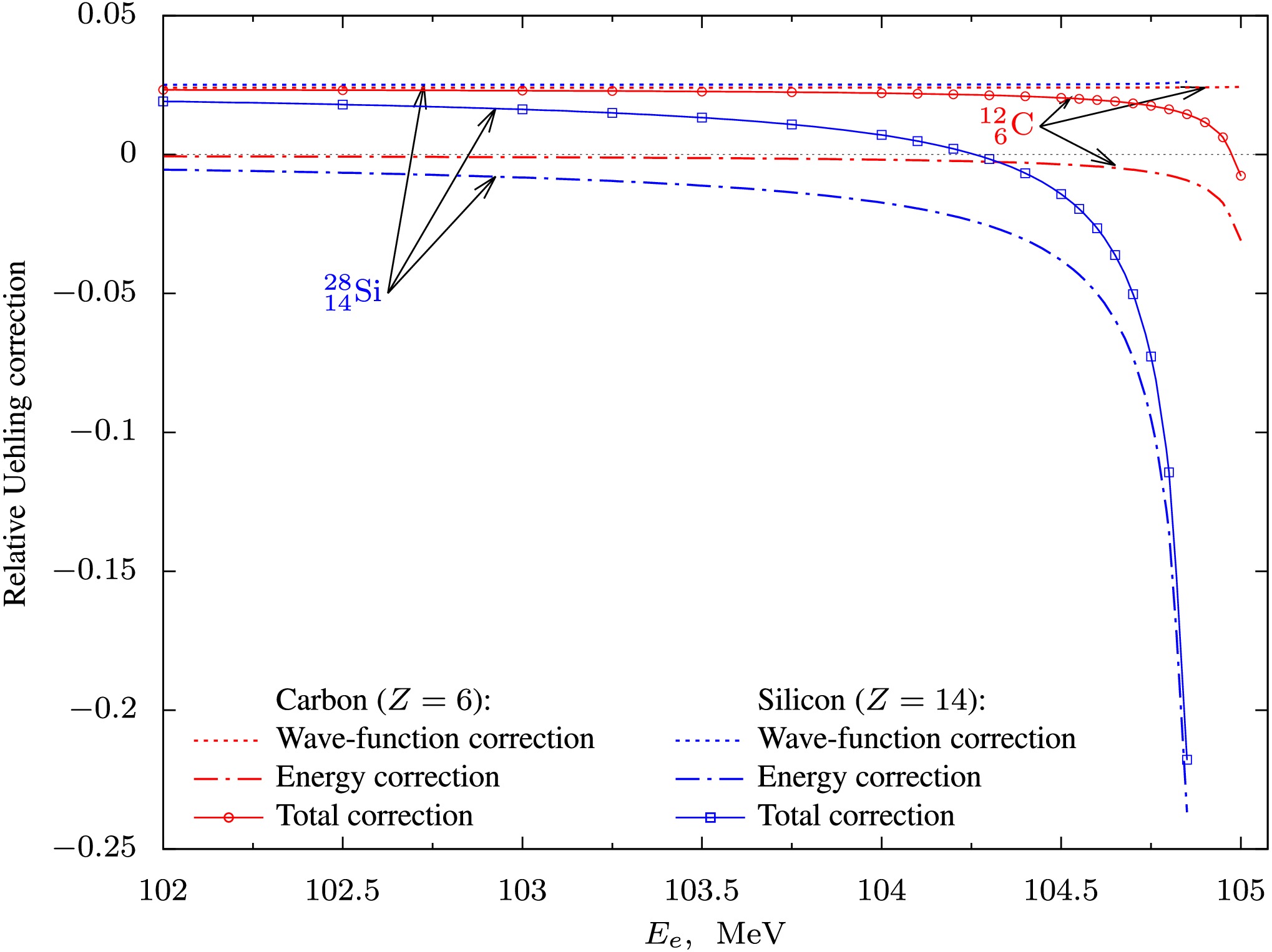
Figure 4. (color online) Relative Uehling corrections to the electron spectrum near the endpoint in the ground-state bound-muon decay process for
$ {}^{12}_{\phantom{1}6}\mathrm{C} $ and$ {}^{28}_{14}\mathrm{Si} $ nuclei. Dotted, dash-dotted, and solid lines correspond to the wave-function, energy, and total corrections, respectively.The WK corrections, shown in Fig. 5, display a different behavior compared to the Ue case. Notably, the wave-function correction
$ \delta^{\mathrm{WK}}_{\mathrm{wf}}\left(E_e\right) $ is no longer similar for$ Z=6 $ and$ Z=14 $ . The corresponding wave-function correction$ \delta^{\mathrm{WK}}_{\mathrm{wf}}\left(E_e\right) $ is about four times larger for$ Z=14 $ than for$ Z=6 $ . Nevertheless, the absolute magnitude of this correction remains negligible, approximately 0.0002% for$ Z=6 $ , which is four orders of magnitude smaller than the Ue correction$ \delta^{\mathrm{Ue}}\left(E_e\right) $ , and approximately 0.005% for$ Z=14 $ . Therefore, the WK contribution to the spectrum can be safely neglected in practical calculations.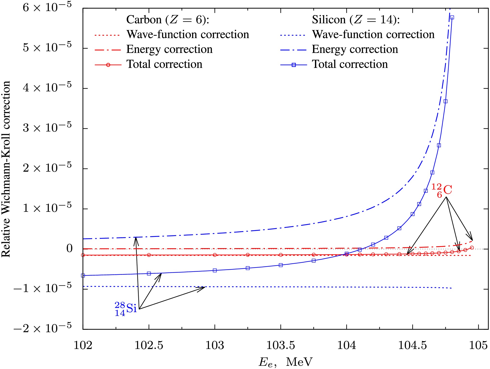
Figure 5. (color online) Relative Wichmann–Kroll corrections to the electron spectrum near the endpoint in the ground-state bound-muon decay process for
$ {}^{12}_{\phantom{1}6}\mathrm{C} $ and$ {}^{28}_{14}\mathrm{Si} $ nuclei. Dotted, dash-dotted, and solid lines correspond to the wave-function, energy, and total corrections, respectively. -
We turn to the final correction affecting wave functions: the electron-screening (SCR) effect. The corresponding results are shown in Fig. 6. In contrast to the FNS and ND corrections, the SCR effect exhibits a completely opposite trend. Specifically, the correction is fully determined by the energy shift, while the wave-function contribution is negligible: less than
$ -0.01 $ % for both$ {}^{12}_{\phantom{1}6}\mathrm{C} $ and$ {}^{28}_{14}\mathrm{Si} $ . Additionally, the wave-function corrections from the SCR effects show practically negligible dependence on the choice of the screening potential. This indicates that, for all considered systems, the SCR effect near the endpoint does not require a self-consistent treatment for the wave functions. Instead, it is sufficient to account for the SCR effect solely through a correction to the endpoint energy.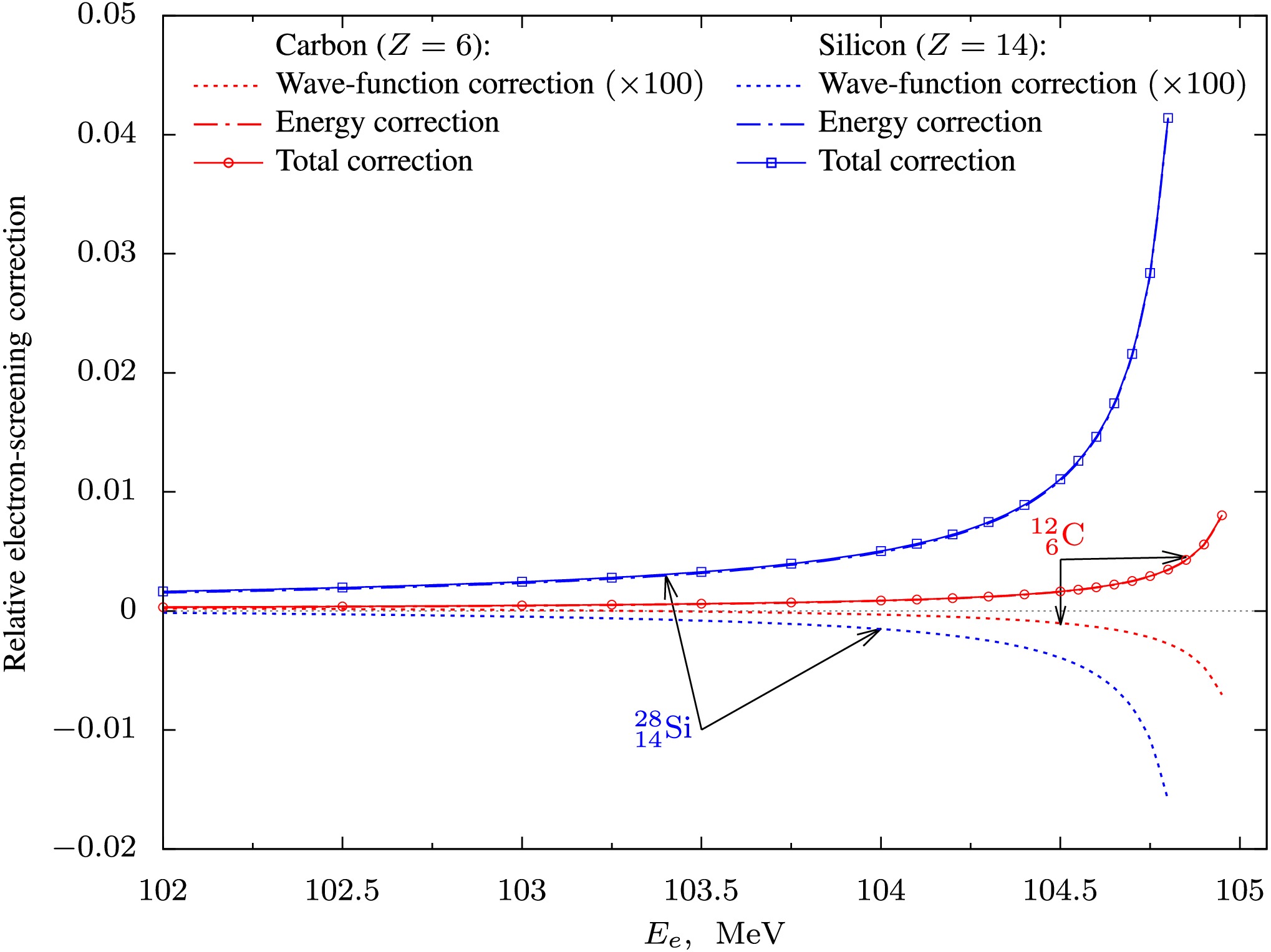
Figure 6. (color online) Relative electron-screening corrections to the electron spectrum near the endpoint in the ground-state bound-muon decay process for
$ {}^{12}_{\phantom{1}6}\mathrm{C} $ and$ {}^{28}_{14}\mathrm{Si} $ nuclei. The dash-dotted lines represents the energy correction, while the dotted lines show the wave-function correction, magnified by a factor of 100 for visibility. The solid lines correspond to the total corrections which closely coincides with the energy corrections. -
In Fig. 7, we present the total corrections to the electron spectra for
$ {}^{12}_{\phantom{1}6}\mathrm{C} $ ,$ {}^{27}_{13}\mathrm{Al} $ , and$ {}^{28}_{14}\mathrm{Si} $ nuclei near the endpoints relative to the corresponding spectra calculated including only the FNS effects. For carbon, the total correction reaches approximately 2.5% in the energy range$ 100\leqslant E_e\leqslant 102.5 $ MeV, where the wave-function corrections dominate. The total correction then rapidly increases up to approximately 4% near$ E_e\approx 104.5 $ MeV, where the energy corrections become more significant. In the case of silicon, the total relative correction is slightly larger, about 2.8%, and remains nearly constant up to$ E_e\approx 104 $ MeV, after which it gradually decreases to 2% as the energy corrections begin to dominate. Aluminum exhibits a distinct behavior: the total relative correction remains nearly constant at approximately 2.5% level until the very endpoint of the spectrum, a behavior anticipated at the beginning of our analysis. From Table 1, one can notice that the various corrections to the muon ground-state energy nearly cancel each other out, leading to a total energy correction of only 3(9) a.u.. As a result, for$ Z=13 $ , the total correction is almost entirely determined by the wave-function modifications.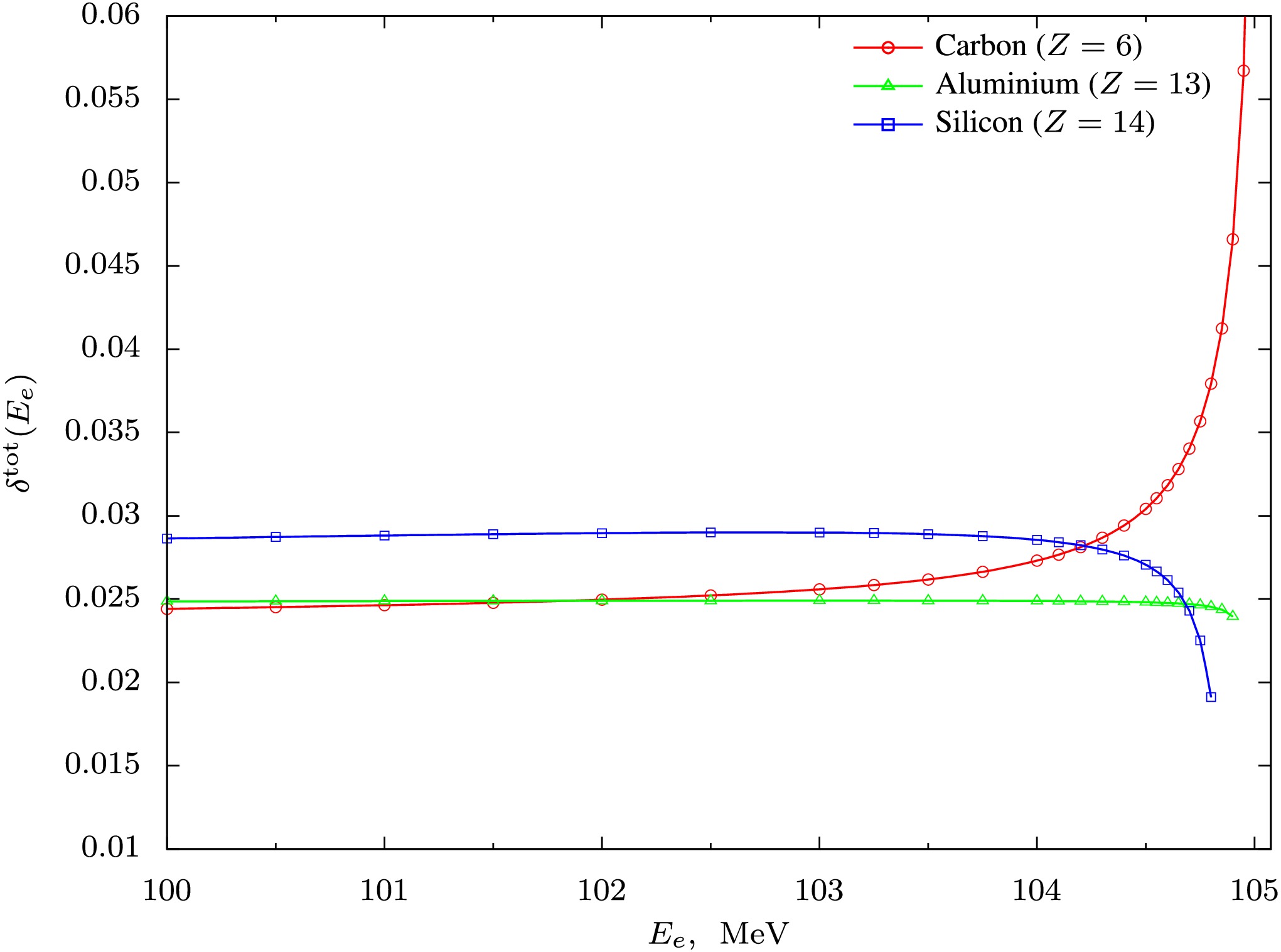
Figure 7. (color online) Total relative corrections to the electron spectra near the endpoints in the bound-muon decay process for
$ {}^{12}_{\phantom{1}6}\mathrm{C} $ ,$ {}^{27}_{13}\mathrm{Al} $ , and$ {}^{28}_{14}\mathrm{Si} $ nuclei. The corrections incorporate simultaneously Uehling, Wichmann–Kroll, nuclear deformation (ND), nuclear recoil, and electron-screening effects and are determined relative to the spectra, which are evaluated with only the FNS effects included. The ND correction is not applied for aluminum.Finally, in Fig. 8, we present the electron spectra for
$ {}^{12}_{\phantom{1}6}\mathrm{C} $ ,$ {}^{27}_{13}\mathrm{Al} $ , and$ {}^{28}_{14}\mathrm{Si} $ , including the FNS, Ue, WK, ND, NR, and SCR effects.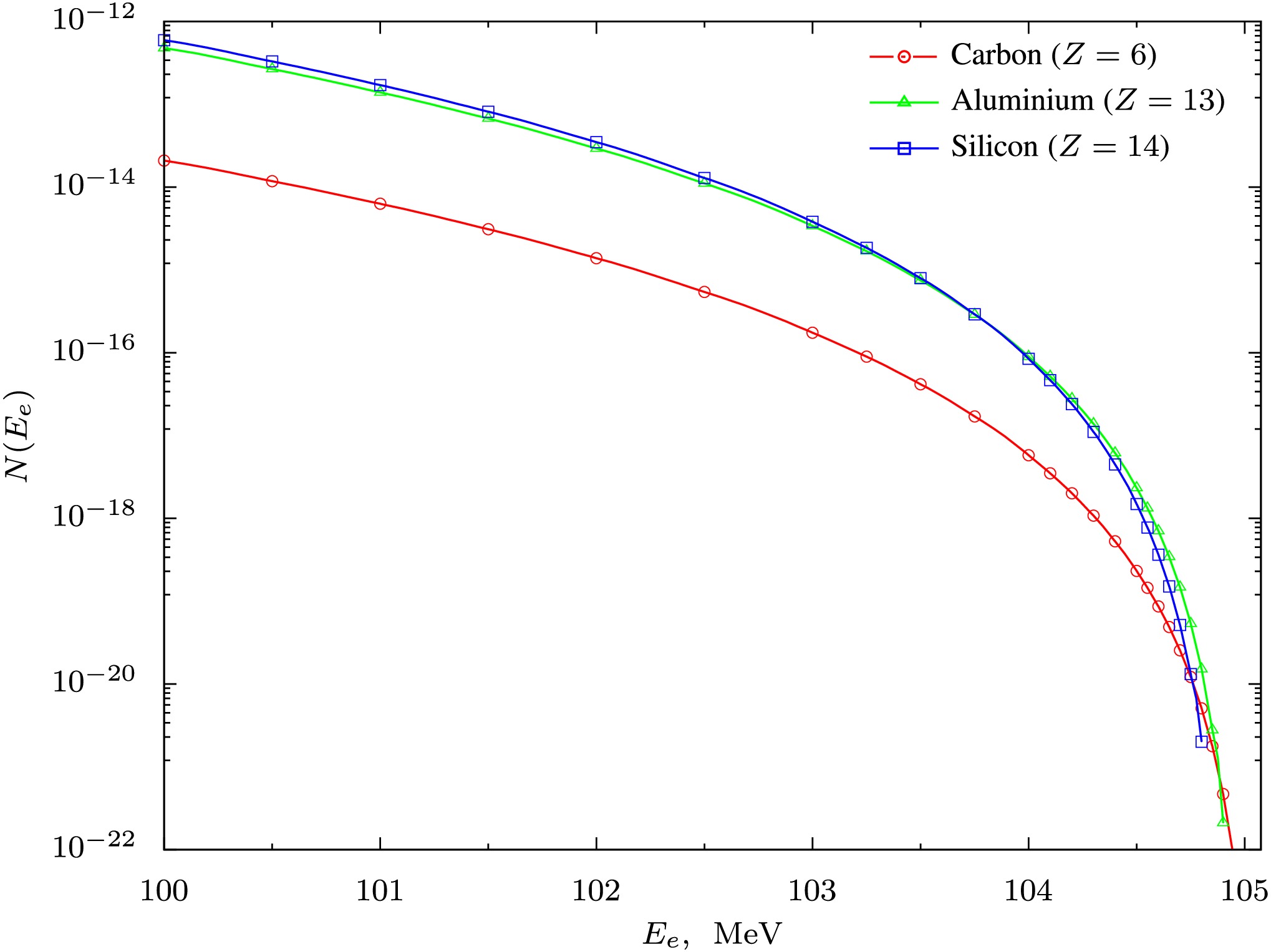
Figure 8. (color online) Electron spectra near the endpoints in the bound-muon decay process for the
$ {}^{12}_{\phantom{1}6}\mathrm{C} $ ,$ {}^{27}_{13}\mathrm{Al} $ , and$ {}^{28}_{14}\mathrm{Si} $ nuclei, calculated with the inclusion of the finite-nuclear-size, Uehling, Wichmann–Kroll, nuclear-deformation (ND), nuclear-recoil, and electron-screening corrections. The ND correction is not applied for aluminum.In summary, our analysis shows that the combined corrections to the electron spectrum due to the nuclear deformation, vacuum polarization, and electron screening may reach approximately 2.5%–5%, depending on the nuclear charge number Z and energy value (see Fig. 7). The magnitudes of some effects, such as nuclear deformation, were a priori unknown, with no previous theoretical estimates available. In the high-energy tail (
$ 100< E_e<105 $ MeV), the relative corrections become significant, but the transition rate itself decreases by about eight orders of magnitude (see Fig. 8). Nevertheless, the nontrivial energy dependence of the atomic corrections near the endpoint of the spectrum might be of practical importance for experimental searches for rare CLFV signals.To separate the CLFV signal of the coherent muon-to-electron conversion in the field of a nucleus,
$ \mu^{-}\to e^{-} $ , from the background in an experiment, one needs statistical modeling. While some backgrounds (e.g., from radiative muon capture or cosmic rays) can be measured, analyzed, and controlled by the experiment, the bound-muon decay,$ \mu^{-}\to e^{-}+\bar{\nu}_{e}+\nu_{\mu} $ , represents an irreducible physical background, which cannot be mitigated by experimental means. For the interpretation of experimental data, it is therefore highly desirable to possess a reliable theoretical prediction for the background channel. Moreover, should a CLFV signal be observed, a precision theoretical description of this background will be indispensable for its quantitative analysis. -
In this study on the bound-muon decay process, we investigated, within the framework of the Fermi effective theory, the influence of various atomic effects on the electron spectrum near its endpoint. We derived two equivalent fully-relativistic expressions for the electron spectrum, corresponding to an arbitrary initial bound-muon state and demonstrated the connection between them, which led to the definite-integral relation involving products of the spherical Bessel functions.
We systematically analyzed the influence of the finite-nuclear-size (FNS), nuclear-deformation, electron-screening (SCR), and vacuum-polarization effects. These corrections were treated self-consistently by incorporating them into both the bound muon and unbound electron wave functions, as well as to the muon binding energy. The nuclear-recoil corrections were also included: for the initial-state muon via the perturbative approach using the non-relativistic mass-shift operator and for the final-state electron via the kinematic approach. The nuclear-deformation correction was implemented following the method of Ref. [35], and the SCR effect was modeled using local, spherically symmetric screening potentials. Notably, no prior comprehensive and self-contained descriptions for the latter two corrections is available. In principle, the developed framework can be also straightforwardly employed to study the influence of the relativistic effects on the bound-muon-decay electron spectrum as well as on the total transition rate of the process. This can be achieved by restoring the parameter c in the obtained expressions (in the units employed,
$ c=1 $ ) and considering the non-relativistic limit$ (c\to\infty) $ . A study of the influence of the relativistic effects on the total decay rate for the muon being in the ground state is reported in Ref. [49].Our analysis focused on the nuclear isotopes
$ {}^{12}_{\phantom{1}6}\mathrm{C} $ ,$ {}^{27}_{13}\mathrm{Al} $ , and$ {}^{28}_{14}\mathrm{Si} $ . We found that the FNS, nuclear-deformation, and vacuum-polarization corrections are mainly determined by self-consistent modifications of the wave functions. Even for small nuclear-charge numbers, such as$ Z=6 $ , the FNS effect must be incorporated into the Dirac equation for both muon and electron. In particular, for carbon, the FNS correction to the spectrum near the endpoint can exceed –40%, highlighting the inadequacy of the point-like nuclear model even for small Z, though it was previously used for$ Z=8 $ in Ref. [26]. The relative nuclear-deformation correction to the endpoint of the spectrum is significant for silicon (0.5%) but negligible for carbon (–0.02%). By contrast, the SCR correction is entirely determined by its effect on the muon ground-state energy, with the wave-function contributions found to be negligible for all the cases considered.Taking all the effects into account, the total correction to the electron spectrum near the endpoint, determined relative to the spectrum obtained considering only the FNS effect, is approximately 2.5% for aluminum, 2.8% for silicon, and up to 5% for carbon. Together with the aforementioned studies, the present work provides a robust theoretical framework for the forthcoming CLFV experiments [7−9], ensuring that systematic uncertainties associated with atomic effects are properly quantified and effectively controlled.
-
The multipole expansion of the two-particle interaction operator
$ V^{\mathrm{F}} $ defined in Eq. (3) can be derived from the multipole expansion of the delta function$ \delta\left( \vec{r}_1 - \vec{r}_2 \right) $ :$ \begin{aligned}[b]&\delta\left(\vec{r}_{1}-\vec{r}_{2}\right)=\sum\limits_{lm}u_{l}\left(r_{1},r_{2}\right)C_{l}^{m}\left(1\right)C_{lm}\left(2\right),\\ &u_{l} \left(r_1,r_2\right)=\frac{\Pi_{l}^{2}}{4\pi}\frac{\delta\left(r_{1}-r_{2}\right)}{r_1 r_2}, \end{aligned} $
(A1) where
$ C_{lm}\left(j\right)=\frac{\sqrt{4\pi}}{\Pi_{l}}Y_{lm}\left(j\right) $
(A2) is the spherical tensor of the rank l,
$ Y_{lm} $ is the spherical harmonic,$ r = \left| \vec{r} \right| $ and$ \Pi_{l_{1}\dots l_{n}}=\sqrt{2l_{1}+1}\dots\sqrt{2l_{n}+1}. $
(A3) Here and hereafter, the sum over l runs from zero to infinity and the sum over m runs in the range
$ -l\leqslant m \leqslant l $ , if not specified otherwise.Instead of the Dirac γ matrices, we employ the α and Σ matrices, which are
$ \alpha^{\rho} = \gamma^0 \gamma^{\rho} $ and$ \Sigma^{\rho} = \alpha^{\rho}\gamma^5 $ . We consider separately the contributions of the time- and space-like components of the corresponding operators,$ \left(\alpha^0,\vec{\alpha}\right) $ and$ \left(\Sigma^0,\vec{\Sigma} \right) $ , and refer to them as the scalar and vector contributions. We treat the time-like operators as spherical tensors of rank 0 and the vector-like operators as spherical tensors of rank 1. Let us separate the scalar,$ V^{\mathrm{s}}_l\left(1,2\right) = u_{l}\left(r_{1},r_{2}\right) \sum\limits_m \left[\alpha^{0} - \Sigma^{0}\right]\left(1\right)[\alpha_{0} - \Sigma_{0}]\left(2\right) C_{l}^{m}\left(1\right)C_{lm}\left(2\right),$
(A4) and the vector,
$ V^{\mathrm{v}}_l\left(1,2\right) = u_{l}\left(r_{1},r_{2}\right) \sum\limits_{mi} \left[\alpha_{1}^{i} - \Sigma^{i}_{1}\right]\left(1\right)\left[\alpha_{1i} - \Sigma_{1i}\right]\left(2\right) C_{l}^{m}\left(1\right)C_{lm}\left(2\right) , $
(A5) parts of the Lorentz scalar in Eq. (3). In Eq. (A5), the index i runs over the set
$ \left(1,2,3\right) $ and subscripts ''1'' for α and Σ refer to the spherical-tensor rank. Introducing some auxiliary operators,$ \begin{aligned}[b] & O_{l}^{1}\left(1,2\right)=\sum\limits_{m}C_{l}^{m}\left(1\right)C_{lm}\left(2\right), \\ & O_{l}^{2}\left(1,2\right)=\sum\limits_{m}\left[\Sigma_{0}C_{l}^{m}\right]\left(1\right)C_{lm}\left(2\right),\\ & O_{l}^{3}\left(1,2\right)=\sum\limits_{m}C_{l}^{m}\left(1\right)\left[\Sigma_{0}C_{lm}\right]\left(2\right), \\ & O_{l}^{4}\left(1,2\right)=\sum\limits_{m}\left[\Sigma_{0}C_{l}^{m}\right]\left(1\right)\left[\Sigma_{0}C_{lm}\right]\left(2\right), \end{aligned} $
(A6) the scalar part of the interaction operator, Eq. (A4), can be written as
$ V_l^{\mathrm{s}}\left(1,2\right) = u_{l}\left(r_{1},r_{2}\right)\left[O_{l}^{1}\left(1,2\right)-O_{l}^{2}\left(1,2\right)-O_{l}^{3}\left(1,2\right)+O_{l}^{4}\left(1,2\right)\right]. $
(A7) Changing the coupling scheme of scalar products in Eq. (A5) [50] and introducing another set of auxiliary operators
$ \begin{aligned}[b] O_{l}^{5}(1,2)=&\sum\limits_{L=l-1}^{l+1}(-1)^{L-l+1}\left(\left[\alpha_{1}(1)\otimes C_{l}(1)\right]_{L}\right.\\ &\left. \cdot\left[\alpha_{1}(2)\otimes C_{l}(2)\right]_{L}\right) ,\\ O_{l}^{6}(1,2)=& \sum\limits_{L=l-1}^{l+1}(-1)^{L-l+1} \left(\left[\Sigma_{1}(1)\otimes C_{l}(1)\right]_{L}\right.\\ &\left.\cdot\left[\alpha_{1}(2)\otimes C_{l}(2)\right]_{L}\right) ,\end{aligned} $
$ \begin{aligned}[b] O_{l}^{7}(1,2)=& \sum\limits_{L=l-1}^{l+1}(-1)^{L-l+1} \left(\left[\alpha_{1}(1)\otimes C_{l}(1)\right]_{L}\right.\\ &\left. \cdot\left[\Sigma_{1}(2)\otimes C_{l}(2)\right]_{L}\right) ,\\ O_{l}^{8}(1,2)=&\sum\limits_{L=l-1}^{l+1}(-1)^{L-l+1}\left(\left[\Sigma_{1}(1)\otimes C_{l}(1)\right]_{L}\right.\\ &\left. \cdot\left[\Sigma_{1}(2)\otimes C_{l}(2)\right]_{L}\right) , \end{aligned} $
(A8) where
$ \left[A \otimes B\right]_{LM} $ denotes the irreducible tensor product of operators, allows us to rewrite the vector part, Eq. (A5), as$ V_l^{\mathrm{v}}\left(1,2\right) = u_{l}\left(r_{1},r_{2}\right)\left[O_{l}^{5}\left(1,2\right)-O_{l}^{6}\left(1,2\right)-O_{l}^{7}\left(1,2\right)+O_{l}^{8}\left(1,2\right)\right]. $
(A9) -
The relativistic four-component wave function in the central-field approximation can be represented in the form [51]
$ \psi_{n\varkappa\mu}\left(\vec{r},\sigma\right)=\left(\begin{array}{c} \psi_{n\varkappa\mu}^{\beta=+1}\left(\vec{r},\sigma\right)\\ \psi_{n\varkappa\mu}^{\beta=-1}\left(\vec{r},\sigma\right) \end{array}\right), $
(B1) where n is the principal quantum number in the bound-state case (it should be replaced with energy E in the unbound-state case), and the index
$ \beta=\left(+1,-1\right) $ enumerates the conventional large,$ \beta=+1 $ , and small,$ \beta=-1 $ , components of the wave function. In turn, the large and small components read as follows:$ \psi_{n\varkappa\mu}^{\beta}\left(\vec{r},\sigma\right)=i^{\frac{\left(1-\beta\right)}{2}}\frac{F_{n\varkappa}^{\beta}\left(r\right)}{r}\chi_{\varkappa\mu}^{\beta}\left(\Omega,\sigma\right), $
(B2) where
$ \chi_{\varkappa\mu}^{\beta}\left(\Omega,\sigma\right)=\left\{ {\begin{array}{*{20}{l}} {{\chi _{ + \varkappa\mu }}\left( {\Omega ,\sigma } \right),}&{\beta = + 1,}\\ {{\chi _{ - \varkappa\mu }}\left( {\Omega ,\sigma } \right),}&{\beta = - 1,} \end{array}} \right. $
(B3) and
$ \chi_{\varkappa\mu}\left(\Omega,\sigma\right) $ is the Pauli spherical spinor.Using Eqs. (A6) and (A7) and our definition of the wave function, (B1) – (B3), for the two-particle matrix elements of the operator
$ V^{\mathrm{s}}_l\left(1,2\right) $ we obtain$\begin{aligned}[b] & \left\langle{cd|V_{l}^{\mathrm{\mathrm{s}}}\left(1,2\right)|ab} \right\rangle \\ = & \frac{\Pi_l^2}{4\pi} \sum\limits_{m} g^{lm}\left(j_{c}\mu_{c};j_{a}\mu_{a}\right)g^{lm}\left(j_{b}\mu_{b};j_{d}\mu_{d}\right) R_{l}^{\mathrm{s}}\left(cd,ab\right),\end{aligned} $
(B4) where
$ g^{lm}\left(j_{1}\mu_{1};j_{2}\mu_{2}\right) $ are the relativistic Gaunt coefficients,$ g^{lm}\left(j_{1}\mu_{1};j_{2}\mu_{2}\right) = \left\langle{\varkappa_1\mu_1|C_{lm}|\varkappa_2\mu_2} \right\rangle , $
(B5) stemmed from the spin-angular integrations, and the radial part is
$ \begin{aligned}[b] R_{l}^{\mathrm{s}}\left(cd,ab\right) =& \sum\limits_{\beta_{1}\beta_{2}}\bigg\{\left[E\left(l,l_{c},l_{a}\right)E\left(l,l_{b},l_{d}\right)R_{1}^{\beta_{1}\beta_{2}}\left(cd,ab\right)\right.\\ &\left. -\beta_{1}\beta_{2}O\left(l,l_{c},l_{a}\right)O\left(l,l_{b},l_{d}\right)R_{4}^{\beta_{1}\beta_{2}}\left(cd,ab\right)\right]\\ & -{\rm i}\left[\beta_{1}O\left(l,l_{c},l_{a}\right)E\left(l,l_{b},l_{d}\right)R_{2}^{\beta_{1}\beta_{2}}\left(cd,ab\right)\right.\\ & \left. +\beta_{2}E\left(l,l_{c},l_{a}\right)O\left(l,l_{b},l_{d}\right)R_{3}^{\beta_{1}\beta_{2}}\left(cd,ab\right)\right]\bigg\}, \end{aligned} $
(B6) where the functions
$\begin{aligned}[b]& E\left(q,w,e\right)=\left\{ {\begin{array}{*{20}{l}} {1,}&{q + w + e{\mkern 1mu} {\mkern 1mu} \quad {\rm{is}}{\mkern 1mu} {\mkern 1mu} {\mkern 1mu} {\rm{even}},}\\ {0,}&{q + w + e{\mkern 1mu} {\mkern 1mu} \quad {\rm{is}}{\mkern 1mu} {\mkern 1mu} {\mkern 1mu} {\rm{odd}},} \end{array}} \right.\\ & O\left( {q,w,e} \right) = \left\{ {\begin{array}{*{20}{l}} {0,}&{q + w + e{\mkern 1mu} {\mkern 1mu} \quad {\rm{is}}{\mkern 1mu} {\mkern 1mu} {\mkern 1mu} {\rm{even}},}\\ {1,}&{q + w + e{\mkern 1mu} {\mkern 1mu} \quad {\rm{is}}{\mkern 1mu} {\mkern 1mu} {\mkern 1mu} {\rm{odd}},} \end{array}} \right. \end{aligned} $
(B7) are introduced. The two-particle radial integrals
$ R_{1-4}^{\beta_{1}\beta_{2}}\left(cd, ab\right) $ in Eq. (B4) are given by$ \begin{aligned}[b] & R_{1}^{\beta_{1}\beta_{2}}\left(cd,ab\right)= \int {\rm d} r\, \left[ F_{n_{c}\varkappa_{c}}^{\beta_{1}}\left(r\right)F_{n_{d}\varkappa_{d}}^{\beta_{2}}\left(r\right) \right]^*\frac{1}{r^{2}}F_{n_{a}\varkappa_{a}}^{\beta_{1}}\left(r\right)F_{n_{b}\varkappa_{b}}^{\beta_{2}}\left(r\right),\\ & R_{2}^{\beta_{1}\beta_{2}}\left(cd,ab\right)= \int {\rm d}r\, \left[ F_{n_{c}\varkappa_{c}}^{\beta_{1}}\left(r\right)F_{n_{d}\varkappa_{d}}^{\beta_{2}}\left(r\right) \right]^*\frac{1}{r^{2}}F_{n_{a}\varkappa_{a}}^{-\beta_{1}}\left(r\right)F_{n_{b}\varkappa_{b}}^{\beta_{2}}\left(r\right),\\ & R_{3}^{\beta_{1}\beta_{2}}\left(cd,ab\right)= \int {\rm d}r\, \left[ F_{n_{c}\varkappa_{c}}^{\beta_{1}}\left(r\right)F_{n_{d}\varkappa_{d}}^{\beta_{2}}\left(r\right) \right]^*\frac{1}{r^{2}}F_{n_{a}\varkappa_{a}}^{\beta_{1}}\left(r\right)F_{n_{b}\varkappa_{b}}^{-\beta_{2}}\left(r\right),\\ & R_{4}^{\beta_{1}\beta_{2}}\left(cd,ab\right)= \int {\rm d}r\, \left[ F_{n_{c}\varkappa_{c}}^{\beta_{1}}\left(r\right)F_{n_{d}\varkappa_{d}}^{\beta_{2}}\left(r\right) \right]^*\frac{1}{r^{2}}F_{n_{a}\varkappa_{a}}^{-\beta_{1}}\left(r\right)F_{n_{b}\varkappa_{b}}^{-\beta_{2}}\left(r\right). \end{aligned} $
(B8) The matrix elements of the operator
$ V^{\mathrm{v}}_l\left(1,2\right) $ can be evaluated using the spin-angular matrix elements of the operator$ [ \sigma_1\otimes C_l]_{LM} $ with the functions$ \chi_{\varkappa\mu}^{\beta}\left(\Omega,\sigma\right) $ [51]:$ \left\langle{\beta\varkappa_{b}\mu_{b}|\left[\sigma_{1}\otimes C_{l}\right]_{LM}|\beta\varkappa_{a}\mu_{a}} \right\rangle = \beta E\left(l,l_{b},l_{a}\right) g^{LM}\left(j_{b}\mu_{b};j_{a}\mu_{a}\right)S_{l}^{\beta}\left(\varkappa_{b};\varkappa_{a}|L\right), $
(B9) $ \left\langle{\beta\varkappa_{b}\mu_{b}|\left[\sigma_{1}\otimes C_{l}\right]_{LM}|-\beta\varkappa_{a}\mu_{a}} \right\rangle =\beta O\left(l,l_{b},l_{a}\right) g^{LM}\left(j_{b}\mu_{b};j_{a}\mu_{a}\right)U_{l}^{\beta}\left(\varkappa_{b};\varkappa_{a}|L\right). $
(B10) These expressions may serve as a definition of the function
$ U_{l}^{\beta}\left(\varkappa_{b};\varkappa_{a}|L\right) $ and$ S_{l}^{\beta}\left(\varkappa_{b};\varkappa_{a}|L\right) $ . One can obtain,$ \left\langle{cd|V_{l}^{\mathrm{\mathrm{v}}}\left(1,2\right)|ab} \right\rangle = -\frac{\Pi_l^2}{4\pi} \sum\limits_{LM} g^{LM}\left(j_{c}\mu_{c};j_{a}\mu_{a}\right)g^{LM}\left(j_{b}\mu_{b};j_{d}\mu_{d}\right)R_{lL}^{\mathrm{v}}\left(cd,ab\right), $
(B11) where
$ \begin{aligned}[b] R_{lL}^{\mathrm{v}}\left(cd,ab\right)= & \sum\limits_{\beta_{1}\beta_{2}} \bigg\{\Big[\beta_{1}\beta_{2}E\left(l,l_{c},l_{a}\right)E\left(l,l_{b},l_{d}\right)S_{l}^{\beta_{1}}\left(\varkappa_{c},\varkappa_{a}|L\right)S_{l}^{\beta_{2}}\left(\varkappa_{b},\varkappa_{d}|L\right)R_{1}^{\beta_{1}\beta_{2}}\left(cd,ab\right)\\ & +O\left(l,l_{c},l_{a}\right)O\left(l,l_{b},l_{d}\right)U_{l}^{\beta_{1}}\left(\varkappa_{c},\varkappa_{a}|L\right)U_{l}^{-\beta_{2}}\left(\varkappa_{b},\varkappa_{d}|L\right)R_{4}^{\beta_{1}\beta_{2}}\left(cd,ab\right)\Big]\\ & + {\rm i} \Big[\beta_{2}O\left(l,l_{c},l_{a}\right)E\left(l,l_{b},l_{d}\right)U_{l}^{\beta_{1}}\left(\varkappa_{c},\varkappa_{a}|L\right)S_{l}^{\beta_{2}}\left(\varkappa_{b},\varkappa_{d}|L\right)R_{2}^{\beta_{1}\beta_{2}}\left(cd,ab\right)\\ & -\beta_{1}E\left(l,l_{c},l_{a}\right)O\left(l,l_{b},l_{d}\right)S_{l}^{\beta_{1}}\left(\varkappa_{c},\varkappa_{a}|L\right)U_{l}^{-\beta_{2}}\left(\varkappa_{b},\varkappa_{d}|L\right)R_{3}^{\beta_{1}\beta_{2}}\left(cd,ab\right)\Big]\bigg\}. \end{aligned} $
(B12) Finally, the matrix element of the Fermi operator can be written as
$ \left\langle{cd|V^{\mathrm{F}}\left(1,2\right)|ab} \right\rangle =\frac{G_{\mathrm{F}}}{\sqrt{2}}\frac{1}{4\pi}\sum\limits_{lmLM}\Pi_{l}^{2}g^{LM}\left(j_{c}\mu_{c};j_{a}\mu_{a}\right)g^{LM}\left(j_{b}\mu_{b};j_{d}\mu_{d}\right)\left[\delta_{Ll}\delta_{Mm}R_{l}^{\mathrm{s}}\left(cd,ab\right)+R_{lL}^{\mathrm{v}}\left(cd,ab\right)\right], $
(B13) where
$ \delta_{ab} $ is the Kronecker delta. -
The amplitude summed over the total angular-momentum projections of all particles can be obtained employing the sum rule for the relativistic Gaunt coefficients:
$ \sum\limits_{\mu_{a}\mu_{b}}g^{lm}\left(j_{b}\mu_{b};j_{a}\mu_{a}\right)g^{kq}\left(j_{b}\mu_{b};j_{a}\mu_{a}\right) = \frac{\Pi_{j_{a}}^{2}}{\Pi_{l}^{2}}\left(C_{l0j_{a}\frac{1}{2}}^{j_{b}\frac{1}{2}}\right)^{2}\delta_{lk}\delta_{mq}. $
(C1) Applying Eq. (C1) to Eq. (B13) results in
$\begin{aligned}[b] \sum\limits_{\mu_{a}\mu_{b}\mu_{c}\mu_{d}}\left|\left\langle{cd|V^{\mathrm{F}}\left(1,2\right)|ab} \right\rangle \right|^{2}=\frac{G_{\mathrm{F}}^{2}}{32\pi^2}\Pi_{j_{a}j_{d}}^{2}\sum\limits_{l}\left(\Pi_{l}C_{l0j_{a}\frac{1}{2}}^{j_{c}\frac{1}{2}}C_{l0j_{d}\frac{1}{2}}^{j_{b}\frac{1}{2}}\right)^{2}\left|R_{l}^{\mathrm{s}}\left(cd,ab\right)+\sum\limits_{L}\frac{\Pi_{L}^{2}}{\Pi_{l}^{2}}R_{Ll}^{\mathrm{v}}\left(cd,ab\right)\right|^{2}. \end{aligned} $
(C2) -
We start from rewriting the expression for the amplitude in the form
$ A=\frac{G_{\mathrm{F}}}{\sqrt{2}}\int {\rm d}\vec{r}M^{\rho}\left(e\mu;\vec{r}\right)M_{\rho}\left(\nu_{\mu}\nu_{e};\vec{r}\right), $
(D1) where
$ M^{\rho}\left(ba;\vec{r}\right) = \int {\rm d}x_{1}\,\delta\left(\vec{r}_{1} - \vec{r}\right)\psi_{b}^{\dagger}\left(x_{1}\right)\gamma^{0}\gamma^{\rho}\left(1 - \gamma^{5}\right)\psi_{a}\left(x_{1}\right) $
(D2) and
$ x\equiv\left(\vec{r},\sigma\right) $ . Using the explicit form of relativistic plane waves,$\begin{aligned}[b] \psi_{E\vec{p}m_{s}}\left(\vec{r},\sigma\right) = & \sqrt{\frac{1}{2E}}\frac{{\rm e}^{{\rm i}\vec{p}\cdot\vec{r}}}{\left(2\pi\right)^{3/2}}u_{\vec{p}m_{s}}\left(\sigma\right),\\ \psi_{-E-\vec{p}m_{s}}\left(\vec{r},\sigma\right) = & \sqrt{\frac{1}{2E}}\frac{{\rm e}^{-{\rm i}\vec{p}\cdot\vec{r}}}{\left(2\pi\right)^{3/2}}v_{\vec{p}m_{s}}\left(\sigma\right), \end{aligned} $
(D3) where
$ E = |E| \gt 0 $ and the bispinors are normalized according to$ u^{\dagger}_{\vec{p}m_{s}}u_{\vec{p}m_{s}}= 2E $ and$ v^{\dagger}_{\vec{p}m_{s}}v_{\vec{p}m_{s}} = 2E $ , one can evaluate the radial integral of the neutrino part$ \begin{aligned}[b] M_{\rho}\left(\nu_{\mu}\nu_{e};\vec{r}\right)=&\frac{1}{\sqrt{2E_{\nu_{e}}2E_{\nu_{\mu}}}}\frac{1}{\left(2\pi\right)^{3}}\int\,{\rm d}\vec{k}\,\delta\left(\vec{k}-\vec{p}_{\nu_{\mu}}-\vec{p}_{\nu_{e}}\right)\\ & \times {\rm e}^{-{\rm i} \vec{k}\cdot\vec{r}}\sum\limits_{\sigma}\overline{u}_{\vec{p}_{\nu_\mu}m_{s_{\nu_\mu}}}\left(\sigma\right)\gamma^{0}\gamma_{\rho}\left(1-\gamma^{5}\right)v_{\vec{p}_{\nu_e}m_{s_{\nu_e}}}\left(\sigma\right).\end{aligned} $
(D4) In Eq. (D4), we have introduced a δ function and related with it integration over some auxiliary three-momentum
$ \vec{k} $ . Substituting Eq. (D4) back to Eq. (D1), the amplitude becomes$ \begin{aligned}[b]A=&\frac{G_{\mathrm{F}}}{\sqrt{2}}\frac{1}{\sqrt{2E_{\nu_{e}}2E_{\nu_{\mu}}}}\frac{1}{\left(2\pi\right)^{3}}\int {\rm d}\vec{k}\,\delta\left(\vec{k}-\vec{p}_{\nu_{\mu}}-\vec{p}_{\nu_{e}}\right)\\ &\times J^{\rho}\left(e\mu;\vec{k}\right)\sum\limits_{\sigma}\overline{u}_{\vec{p}_{\mu}m_{s_{\mu}}}\left(\sigma\right)\gamma^{0}\gamma_{\rho}\left(1-\gamma^{5}\right)v_{\vec{p}_{e}m_{s_{e}}}\left(\sigma\right), \end{aligned} $
(D5) where
$ J^{\rho}\left(e\mu;\vec{k}\right) $ is the effective lepton current defined in Eq. (10). We can now evaluate the absolute value of the amplitude squared and summed over the spin projections on the direction of$ \vec{p} $ of undetected neutrinos$ \sum\limits_{m_{s_{e}}m_{s_{\mu}}}\left|A\right|^{2}=\frac{G_{\mathrm{F}}^{2}}{2}\frac{1}{\left(2\pi\right)^{6}}\int\,{\rm d}\vec{k}\,\delta\left(\vec{k}-\vec{p}_{\nu_{\mu}}-\vec{p}_{\nu_{e}}\right)L_{\alpha\beta}\left(\vec{k}\right)\frac{N^{\alpha\beta}}{4E_{\nu_{\mu}}E_{\nu_{e}}}, $
(D6) where the lepton tensor is
$ L_{\alpha\beta}\left(e\mu;\vec{k}\right)=J_{\alpha}\left(e\mu;\vec{k}\right)J_{\beta}^{\dagger}\left(e\mu;\vec{k}\right) $
(D7) and the neutrino tensor is
$ N^{\alpha\beta}=8\left(-g^{\alpha\beta}g_{\rho\tau}p_{\nu_{e}}^{\rho}p_{\nu_{\mu}}^{\tau}+p_{\nu_{e}}^{\alpha}p_{\nu_{\mu}}^{\beta}+p_{\nu_{e}}^{\beta}p_{\nu_{\mu}}^{\alpha}+ {\rm i} \varepsilon^{\alpha\beta\rho\tau}p_{\nu_{e}\rho}p_{\nu_{\mu}\tau}\right). $
(D8) To write down the expression for the differential probability, we form the four-dimensional delta function over the intermediate four-momentum k and obtain
$ \begin{aligned}[b] {\rm d} W\left(\zeta_{e},\zeta_{\mu}\right)=&\frac{G_{\mathrm{F}}^{2}}{2}\frac{1}{\left(2\pi\right)^{5}}\int\,{\rm d}k\,{\rm d}\vec{p}_{\nu_{e}}\,d\vec{p}_{\nu_{\mu}}\,{\rm d}E_{e}\,\delta\left(E_{\mu}-E_{e}-k^{0}\right)\\ & \times \delta\left(k-p_{\nu_{\mu}}-p_{\nu_{e}}\right)L_{\alpha\beta}\left(e\mu;\vec{k}\right)\frac{N^{\alpha\beta}}{4E_{\nu_{\mu}}E_{\nu_{e}}}. \end{aligned} $
(D9) The integration over the three-momenta of neutrinos is performed using the formula
$ \int {\rm d}\vec{p}_{\nu_{e}}\,{\rm d}\vec{p}_{\nu_{\mu}}\,\frac{\delta\left(k-p_{\nu_{\mu}}-p_{\nu_e}\right)N^{\alpha\beta}}{4E_{\nu_{e}}E_{\nu_{\mu}}}=\frac{4\pi}{3}\left(-g^{\alpha\beta}k^{2}+k^{\alpha}k^{\beta}\right). $
(D10) Finally, we assemble the expression for the electron spectrum within the one-particle effective approach
$ \begin{aligned}[b]\frac{{\rm d}W\left(E_{e},n_{\mu}\varkappa_{\mu}\right)}{{\rm d}E_{e}}=&\frac{G_{\mathrm{F}}^{2}}{2}\frac{1}{\left(2\pi\right)^{5}}\frac{4\pi}{3}\frac{1}{\Pi_{j_{\mu}}^{2}}\sum\limits_{\mu_{\mu}}\sum\limits_{\varkappa_{e}\mu_{e}}\int {\rm d}\vec{k}\,\\ & \times L_{\alpha\beta} \left(e\mu;\vec{k}\right)\left(-g^{\alpha\beta}k^{2}+k^{\alpha}k^{\beta}\right),\end{aligned} $
(D11) where
$ k^{0}=E_{\mu}-E_{e} $ . -
The multipole expansion of the effective current is based on the following expansion of the exponent
$ {\rm e}^{-{\rm i} \vec{k}\cdot\vec{r}} = \sqrt{4\pi}\sum\limits_{lm}\Pi_{l}i^{-l}j_{l}\left(kr\right)C_{lm}\left(\hat{r}\right)Y_{lm}^{*}\left(\hat{k}\right), $
(E1) where
$ \hat{n} = \vec{n}/|\vec{n}| $ . This leads to$ J_{\rho}\left(ba;\vec{k}\right)=\sqrt{4\pi}\sum\limits_{lm}\Pi_{l}i^{-l}Y_{lm}^{*}\left(\hat{k}\right)J_{\rho,lm}\left(ba;k\right), $
(E2) where the
$ lm $ -th partial-wave component of the effective current is$ J_{\rho,lm}\left(ba;k\right)\equiv\left\langle{b|\left(\alpha_{\rho}-\Sigma_{\rho}\right)j_{l}\left(kr\right)C_{lm}|a} \right\rangle . $
(E3) We emphasize that here ρ is the Lorentz index but m is the cyclic index (it indicates the component of the corresponding spherical tensor).
The matrix elements of the partial-wave components of the effective current can be evaluated using the results of Appendix B. One can obtain for the scalar part,
$ \rho=0 $ ,$ \begin{aligned}[b]J_{0,lm}\left(ba;k\right)=&g^{lm}\left(j_{b}\mu_{b};j_{a}\mu_{a}\right)\bigg[E\left(l_{b},l_{a},l\right)\sum\limits_{\beta}R^{\beta\beta}\left(ba;j_{l}\right) \\ & -{\rm i}O\left(l_{b},l_{a},l\right)\sum\limits_{\beta}\beta R^{\beta-\beta}\left(ba;j_{l}\right)\bigg] \end{aligned} $
(E4) and for the vector part,
$ \rho=t $ ,$ t=1,2,3 $ ,$ \begin{aligned}[b]J_{t,lm}\left(ba;k\right)=& \sum\limits_{LM}C_{1tlm}^{LM}g^{LM}\left(j_{b}\mu_{b};j_{a}\mu_{a}\right) \\ &\times \left[-E\left(l_{b},l_{a},l\right)\sum\limits_{\beta}\beta S_{l}^{\beta}\left(\varkappa_{b},\varkappa_{a}|L\right)R^{\beta\beta}\left(ba;j_{l}\right)\right.\\ & \left. +{\rm i} O\left(l_{b},l_{a},l\right)\sum\limits_{\beta}U_{l}^{\beta}\left(\varkappa_{b},\varkappa_{a}|L\right)R^{\beta-\beta}\left(ba;j_{l}\right)\right], \end{aligned} $
(E5) where the one-particle radial integrals are given by
$ R^{\beta_{1}\beta_{2}}\left(ba;j_{l}\right)=\int_0^{\infty}\left[F_{n_b\varkappa_b}^{\beta_{1}}\left(r\right)\right]^{*} j_{l}\left(kr\right)F_{n_a\varkappa_a}^{\beta_{2}}\left(r\right)\,{\rm d}r. $
(E6) -
The angular integration in Eq. (D11) can be performed for the spherical components of the vector
$ \vec{k} $ using the Clebsch-Gordan expansion for products of spherical harmonics and the well-known expression for the integrals of products of spherical harmonics over the solid angle. Executing the steps mentioned above, we represent the resulting integration over the angular coordinates in the following form$ \begin{aligned}[b] \int\,{\rm d}\vec{k}\,L_{\alpha\beta} \left(ba;\vec{k}\right)\left(-g^{\alpha\beta}k^{2}+k^{\alpha}k^{\beta}\right)=& 4\pi \sum\limits_{LM}g^{LM}\left(j_{b}\mu_{b};j_{a}\mu_{a}\right)g^{LM}\left(j_{b}\mu_{b};j_{a}\mu_{a}\right) \int {\rm d}k\,k^{2}\Big\{ k^{2}R_{L}^{\mathrm{ss}}\left(ba;k\right)-2k^{0}k\mathrm{Re}R_{L}^{\mathrm{sv}}\left(ba;k\right)\\ & +\left[\left(k^{0}\right)^{2}-k^{2}\right]R_{L}^{\mathrm{vv,1}}\left(ba;k\right)+k^{2}R_{L}^{\mathrm{vv,2}}\left(ba;k\right)\Big\}. \end{aligned} $
(F1) The scalar-scalar (ss), scalar-vector (sv), and vector-vector diagonal (vv,1), and vector-vector non-diagonal (vv,2) radial integrals are given by
$ R_{L}^{\mathrm{ss}}\left(ba;k\right)=\Pi_{L}^{2}\left| \sum\limits_{\beta}\left[E\left(l_{b},l_{a},L\right)R^{\beta\beta}\left(ba;j_{L}\right)-{\rm i}O\left(l_{b},l_{a},L\right)\beta R^{\beta-\beta}\left(ba;j_{L}\right)\right]\right|^{2}, $
(F2) $ \begin{aligned}[b] R_{L}^{\mathrm{sv}}\left(ba;k\right)=&\sum\limits_{l} i^{L-l}\Pi_{lL}C_{L010}^{l0}\sum\limits_{\beta}\left[E\left(l_{b},l_{a},L\right)R^{\beta\beta}\left(ba;j_{L}\right)+ {\rm i}O\left(l_{b},l_{a},L\right)\beta R^{\beta-\beta}\left(ba;j_{L}\right)\right]\\ & \times \left[E\left(l_{b},l_{a},l\right)\sum\limits_{\beta}\beta S_{l}^{\beta}\left(\varkappa_{b},\varkappa_{a}|L\right)R^{\beta\beta}\left(ba;j_{l}\right)-{\rm i}O\left(l_{b},l_{a},l\right)\sum\limits_{\beta}U_{l}^{\beta}\left(\varkappa_{b},\varkappa_{a}|L\right)R^{\beta-\beta}\left(ba;j_{l}\right)\right], \end{aligned} $
(F3) $ R_{L}^{\mathrm{vv},1}\left(ba;k\right)=\sum\limits_{l}\Pi_{l}^{2}\left|\left[-E\left(l_{b},l_{a},l\right)\sum\limits_{\beta}\beta S_{l}^{\beta}\left(\varkappa_{b},\varkappa_{a}|L\right)R^{\beta\beta}\left(ba;j_{l}\right)+{\rm i}O\left(l_{b},l_{a},l\right)\sum\limits_{\beta}U_{l}^{\beta}\left(\varkappa_{b},\varkappa_{a}|L\right)R^{\beta-\beta}\left(ba;j_{l}\right)\right]\right|^{2}, $
(F4) $ \begin{aligned}[b] R_{L}^{\mathrm{vv},2}\left(ba;k\right)=& \sum\limits_{l_{1}l_{2}}i^{-l_{1}+l_{2}}\Pi_{l_{1}l_{2}}C_{L010}^{l_{2}0}C_{L010}^{l_{1}0}\\ &\times \left[E\left(l_{b},l_{a},l_{1}\right)\sum\limits_{\beta}\beta S_{l_{1}}^{\beta}\left(\varkappa_{b},\varkappa_{a}|L\right)R^{\beta\beta}\left(ba;j_{l_{1}}\right)-{\rm i}O\left(l_{b},l_{a},l_{1}\right)\sum\limits_{\beta}U_{l_{1}}^{\beta}\left(\varkappa_{b},\varkappa_{a}|L\right)R^{\beta-\beta}\left(ba;j_{l_{1}}\right)\right]\\ & \times \left[E\left(l_{b},l_{a},l_{2}\right)\sum\limits_{\beta}\beta S_{l_{2}}^{\beta}\left(\varkappa_{b},\varkappa_{a}|L\right)R^{\beta\beta}\left(ba;j_{l_{2}}\right)+{\rm i}O\left(l_{b},l_{a},l_{2}\right)\sum\limits_{\beta}U_{l_{2}}^{\beta}\left(\varkappa_{b},\varkappa_{a}|L\right)R^{\beta-\beta}\left(ba;j_{l_{2}}\right)\right]. \end{aligned} $
(F5) Finally, the triple sum over the total angular-momentum projections of particles a and b and the sum over intermediate angular momentum projections M is evaluated using the sum rules for the relativistic Gaunt coefficients, Eq. (C1). The result is
$ \begin{aligned}[b]\sum\limits_{M\mu_{b}\mu_{a}}\int\,{\rm d}\vec{k}\,L_{\alpha\beta}\left(ba;\vec{k}\right)\left(-g^{\alpha\beta}k^{2}+k^{\alpha}k^{\beta}\right) =& 4\pi\Pi_{j_{b}}^{2}\sum\limits_{L} \left(C_{j_{b}\frac{1}{2}L0}^{j_{a}\frac{1}{2}}\right)^{2}\int_0^{k^0} {\rm d}k\,k^{2}\Big\{ k^{2}R_{L}^{\mathrm{ss}}\left(ba;k\right)-2k^{0}k\mathrm{Re}R_{L}^{\mathrm{sv}}\left(ba;k\right)\\ & +\left[\left(k^{0}\right)^{2}-k^{2}\right]R_{L}^{\mathrm{vv},1}\left(ba;k\right)+k^{2}R_{L}^{\mathrm{vv},2}\left(ba;k\right)\Big\}. \end{aligned} $
(F6) -
We start by equating the right-hand sides of Eqs. (9) and (11) and restrict ourselves with a comparison of the scalar contribution only. For our purposes, the explicit form of the central-field radial wave functions for a massless particle,
$ E>0 $ , and antiparticle,$ E<0 $ , are needed$ F_{E\varkappa}^{\beta}\left(r\right)=\frac{1}{c}\sqrt{\frac{E^{2}}{\pi}} \times \left\{ {\begin{array}{*{20}{l}} {r{j_l}\left( {Er} \right),}&{\beta = + 1,}\\ {{S_E}{S_{{_d}}}r{j_{\bar l}}\left( {Er} \right),}&{\beta = - 1,} \end{array}} \right. $
(G1) where
$ S_{x}= \mathrm{sgn}(x) $ and$ \overline{l}=\left|-\varkappa+\dfrac{1}{2}\right|-\dfrac{1}{2} $ . It should be noted that the following relation between the radial components of the wave function for a massless particle holds$ F_{E-\varkappa}^{\beta}\left(r\right)=S_{E}S_{\varkappa}\beta F_{E\varkappa}^{-\beta}\left(r\right). $
(G2) Without loss of generality, let us fix states a, c, and the l-th term of the multipole sum and consider the case
$ E\left(l,l_a,l_c\right)=1 $ . We spin off Eq. (9) employing the definition of the two-particle radial integrals, Eqs. (B8), changing the order of the radial and energy integration, and pulling aside everything that depends on states a and c. After these manipulations, Eq. (9) becomes proportional to$ \begin{aligned}[b]\frac{{\rm d}W^{2\mathrm{p}}\left(E_{e},n_{\mu}\varkappa_{\mu}\right)}{{\rm d}E_{e}}\propto & \frac{1}{16\pi}\int_{0}^{\Delta}{\rm d}E_{d}\,\sum\limits_{\varkappa_{d}\varkappa_{b}}\left(\Pi_{j_{d}}C_{l0j_{d}\frac{1}{2}}^{j_{b}\frac{1}{2}}\right)^{2} \Bigg\{ \bigg[ E\left(l,l_{b},l_{d}\right)\sum\limits_{\beta}\left(F_{E_{d}\varkappa_{d}}^{\beta}\left(r_{1}\right)\right)^{*}F_{-\left(\Delta-E_{d}\right)\varkappa_{b}}^{\beta}\left(r_{1}\right) \\ &+{\rm i}O\left(l,l_{b},l_{d}\right)\sum\limits_{\beta}\beta\left(F_{E_{d}\varkappa_{d}}^{\beta}\left(r_{1}\right)\right)^{*}F_{-\left(\Delta-E_{d}\right)\varkappa_{b}}^{-\beta}\left(r_{1}\right)\bigg] \bigg[E\left(l,l_{b},l_{d}\right)\sum\limits_{\beta}\left(F_{E_{d}\varkappa_{d}}^{\beta}\left(r_{2}\right)\right)^{*}F_{-\left(\Delta-E_{d}\right)\varkappa_{b}}^{\beta}\left(r_{2}\right)\\ & +{\rm i} O\left(l,l_{b},l_{d}\right)\sum\limits_{\beta}\beta\left(F_{E_{d}\varkappa_{d}}^{\beta}\left(r_{2}\right)\right)^{*}F_{-\left(\Delta-E_{d}\right)\varkappa_{b}}^{-\beta}\left(r_{2}\right)\bigg]^{*}\Bigg\}. \end{aligned} $
(G3) With the aid of Eq. (G2), we note that Eq. (G3) is invariant under the change
$ \varkappa\to-\varkappa $ . Therefore, for each$ |\varkappa| $ one can sum over the signs of$ \varkappa $ ; this results leads to an additional factor of$ 4 $ . On the other hand, from Eq. (11) we obtain$ \frac{{\rm d}W^{1\mathrm{p}}\left(E_{e},n_{\mu}\varkappa_{\mu}\right)}{{\rm d}E_{e}}\propto\frac{1}{12\pi^{3}}\int_{0}^{\Delta}{\rm d}k\,k^{4} j_{l}\left(kr_{1}\right)j_{l}^{*}\left(kr_{2}\right). $
(G4) Let us introduce
$ j_{pq}\left(z,y;x\right)=j_{p}\left(yx\right)j_{q}\left(y\left(z-x\right)\right), $
(G5) Then, for
$ \alpha,\beta,\gamma>0 $ and$ j_{s}=s-\dfrac{1}{2} $ we obtain$ \begin{aligned}[b]\int_{0}^{\alpha}{\rm d}x\,x^{4}j_{l}\left(\beta x\right)j_{l}\left(\gamma x\right)=& 3\sum\limits_{pq}\left(\Pi_{j_{q}}C_{j_{q}\frac{1}{2}l0}^{j_{p}\frac{1}{2}}\right)^{2}\int_{0}^{\alpha}{\rm d}x\,x^{2}\left(\alpha-x\right)^{2}\\ &\times \bigg\{ E\left(l,p,q\right)\left[j_{pq}\left(\alpha,\beta;x\right)-j_{p-1q-1}\left(\alpha,\beta;x\right)\right]\left[j_{pq}\left(\alpha,\gamma;x\right)-j_{p-1q-1}\left(\alpha,\gamma;x\right)\right]\\ & + O\left(l,p,q\right)\left[j_{pq-1}\left(\alpha,\beta;x\right)+j_{p-1q}\left(\alpha,\beta;x\right)\right]\left[j_{pq-1}\left(\alpha,\gamma;x\right)+j_{p-1q}\left(\alpha,\gamma;x\right)\right]\bigg\}. \end{aligned} $
(G6) The validity of this equation is confirmed numerically. It is possible to further simplify this relation by using properties of the Clebsch-Gordan coefficients
$ \begin{aligned}[b] \int_{0}^{\alpha}{\rm d}x\,x^{4}j_{l}\left(\beta x\right)j_{l}\left(\gamma x\right)=&\frac{3}{\left(2l+1\right)}\sum\limits_{pq}\int_{0}^{\alpha}{\rm d}x\,x^{2}\left(\alpha-x\right)^{2}\\ &\times \Bigg\{\left(p+q-l\right)\left(p+q+l+1\right)\left(C_{q0\,p0}^{l0}\right)^{2}\left[j_{pq}\left(\alpha,\beta;x\right)-j_{p-1q-1}\left(\alpha,\beta;x\right)\right]\left[j_{pq}\left(\alpha,\gamma;x\right)-j_{p-1q-1}\left(\alpha,\gamma;x\right)\right]\\ &-\left(p-q-l\right)\left(p-q+l+1\right)\left(C_{q-10\,p0}^{l0}\right)^{2}\left[j_{pq-1}\left(\alpha,\beta;x\right)+j_{p-1q}\left(\alpha,\beta;x\right)\right]\left[j_{pq-1}\left(\alpha,\gamma;x\right)+j_{p-1q}\left(\alpha,\gamma;x\right)\right]\Bigg\}. \end{aligned} $
(G7) Using the expansion of Eq. (G7) as
$ \gamma\to0 $ and the asymptotic behavior of the spherical Bessel function,$ j_{n}\left(z\right)\stackrel{z\to0}{\sim}\frac{z^{n}}{\left(2n+1\right)!!}, $
(G8) yields
$ \begin{aligned}[b] \int_{0}^{\alpha}{\rm d}x\,x^{l+4}j_{l}\left(\beta x\right)=&-3\left(2l-1\right)!!\sum\limits_{pq}\int_{0}^{\alpha}{\rm d}x\,\frac{x^{p+1}\left(\alpha-x\right)^{q+1}}{\left(2p-1\right)!!\left(2q-1\right)!!}\\ &\times \Bigg\{\left(p+q-l\right)\left(p+q+l+1\right)\left(C_{q0\,p0}^{l0}\right)^{2}\left[j_{pq}\left(\alpha,\beta;x\right)-j_{p-1q-1}\left(\alpha,\beta;x\right)\right]\delta_{p+q,l+2}\\ & +\left(p-q-l\right)\left(p-q+l+1\right)\left(C_{q-10\,p0}^{l0}\right)^{2}\left[j_{pq-1}\left(\alpha,\beta;x\right)+j_{p-1q}\left(\alpha,\beta;x\right)\right]\left(\frac{x}{2p+1}+\frac{\alpha-x}{2q+1}\right)\delta_{p+q,l+1}\Bigg\}. \end{aligned} $
(G9) An additional expansion in β results in relations for sums of the Clebsch-Gordan coefficients:
$ \frac{1}{2l+1}\frac{\left(2l+4\right)!}{\left[\left(2l-1\right)!!\right]^{2}} =6\sum\limits_{pq}\frac{\left(2p\right)!\left(2q\right)!}{\left[\left(2p-1\right)!!\left(2q-1\right)!!\right]^{2}} \left[\left(2l+3\right)\left(C_{q0\,p0}^{l0}\right)^{2}\delta_{p+q,l+2}+2p\left(2q-1\right)\left(2+\frac{1}{2p+1}\right)\left(C_{q-10\,p0}^{l0}\right)^{2}\delta_{p+q,l+1}\right]. $
(G10) -
We start by equating the right-hand sides of Eqs. (9) and (11) and restrict ourselves with a comparison of the scalar contribution only. For our purposes, the explicit form of the central-field radial wave functions for a massless particle,
$ E>0 $ , and antiparticle,$ E<0 $ , are needed$ F_{E\varkappa}^{\beta}\left(r\right)=\frac{1}{c}\sqrt{\frac{E^{2}}{\pi}} \times \left\{ {\begin{array}{*{20}{l}} {r{j_l}\left( {Er} \right),}&{\beta = + 1,}\\ {{S_E}{S_{{_d}}}r{j_{\bar l}}\left( {Er} \right),}&{\beta = - 1,} \end{array}} \right. $
(G1) where
$ S_{x}= \mathrm{sgn}(x) $ and$ \overline{l}=\left|-\varkappa+\dfrac{1}{2}\right|-\dfrac{1}{2} $ . It should be noted that the following relation between the radial components of the wave function for a massless particle holds$ F_{E-\varkappa}^{\beta}\left(r\right)=S_{E}S_{\varkappa}\beta F_{E\varkappa}^{-\beta}\left(r\right). $
(G2) Without loss of generality, let us fix states a, c, and the l-th term of the multipole sum and consider the case
$ E\left(l,l_a,l_c\right)=1 $ . We spin off Eq. (9) employing the definition of the two-particle radial integrals, Eqs. (B8), changing the order of the radial and energy integration, and pulling aside everything that depends on states a and c. After these manipulations, Eq. (9) becomes proportional to$ \begin{aligned}[b]\frac{{\rm d}W^{2\mathrm{p}}\left(E_{e},n_{\mu}\varkappa_{\mu}\right)}{{\rm d}E_{e}}\propto & \frac{1}{16\pi}\int_{0}^{\Delta}{\rm d}E_{d}\,\sum\limits_{\varkappa_{d}\varkappa_{b}}\left(\Pi_{j_{d}}C_{l0j_{d}\frac{1}{2}}^{j_{b}\frac{1}{2}}\right)^{2} \Bigg\{ \bigg[ E\left(l,l_{b},l_{d}\right)\sum\limits_{\beta}\left(F_{E_{d}\varkappa_{d}}^{\beta}\left(r_{1}\right)\right)^{*}F_{-\left(\Delta-E_{d}\right)\varkappa_{b}}^{\beta}\left(r_{1}\right) \\ &+{\rm i}O\left(l,l_{b},l_{d}\right)\sum\limits_{\beta}\beta\left(F_{E_{d}\varkappa_{d}}^{\beta}\left(r_{1}\right)\right)^{*}F_{-\left(\Delta-E_{d}\right)\varkappa_{b}}^{-\beta}\left(r_{1}\right)\bigg] \bigg[E\left(l,l_{b},l_{d}\right)\sum\limits_{\beta}\left(F_{E_{d}\varkappa_{d}}^{\beta}\left(r_{2}\right)\right)^{*}F_{-\left(\Delta-E_{d}\right)\varkappa_{b}}^{\beta}\left(r_{2}\right)\\ & +{\rm i} O\left(l,l_{b},l_{d}\right)\sum\limits_{\beta}\beta\left(F_{E_{d}\varkappa_{d}}^{\beta}\left(r_{2}\right)\right)^{*}F_{-\left(\Delta-E_{d}\right)\varkappa_{b}}^{-\beta}\left(r_{2}\right)\bigg]^{*}\Bigg\}. \end{aligned} $
(G3) With the aid of Eq. (G2), we note that Eq. (G3) is invariant under the change
$ \varkappa\to-\varkappa $ . Therefore, for each$ |\varkappa| $ one can sum over the signs of$ \varkappa $ ; this results leads to an additional factor of$ 4 $ . On the other hand, from Eq. (11) we obtain$ \frac{{\rm d}W^{1\mathrm{p}}\left(E_{e},n_{\mu}\varkappa_{\mu}\right)}{{\rm d}E_{e}}\propto\frac{1}{12\pi^{3}}\int_{0}^{\Delta}{\rm d}k\,k^{4} j_{l}\left(kr_{1}\right)j_{l}^{*}\left(kr_{2}\right). $
(G4) Let us introduce
$ j_{pq}\left(z,y;x\right)=j_{p}\left(yx\right)j_{q}\left(y\left(z-x\right)\right), $
(G5) Then, for
$ \alpha,\beta,\gamma>0 $ and$ j_{s}=s-\dfrac{1}{2} $ we obtain$ \begin{aligned}[b]\int_{0}^{\alpha}{\rm d}x\,x^{4}j_{l}\left(\beta x\right)j_{l}\left(\gamma x\right)=& 3\sum\limits_{pq}\left(\Pi_{j_{q}}C_{j_{q}\frac{1}{2}l0}^{j_{p}\frac{1}{2}}\right)^{2}\int_{0}^{\alpha}{\rm d}x\,x^{2}\left(\alpha-x\right)^{2}\\ &\times \bigg\{ E\left(l,p,q\right)\left[j_{pq}\left(\alpha,\beta;x\right)-j_{p-1q-1}\left(\alpha,\beta;x\right)\right]\left[j_{pq}\left(\alpha,\gamma;x\right)-j_{p-1q-1}\left(\alpha,\gamma;x\right)\right]\\ & + O\left(l,p,q\right)\left[j_{pq-1}\left(\alpha,\beta;x\right)+j_{p-1q}\left(\alpha,\beta;x\right)\right]\left[j_{pq-1}\left(\alpha,\gamma;x\right)+j_{p-1q}\left(\alpha,\gamma;x\right)\right]\bigg\}. \end{aligned} $
(G6) The validity of this equation is confirmed numerically. It is possible to further simplify this relation by using properties of the Clebsch-Gordan coefficients
$ \begin{aligned}[b] \int_{0}^{\alpha}{\rm d}x\,x^{4}j_{l}\left(\beta x\right)j_{l}\left(\gamma x\right)=&\frac{3}{\left(2l+1\right)}\sum\limits_{pq}\int_{0}^{\alpha}{\rm d}x\,x^{2}\left(\alpha-x\right)^{2}\\ &\times \Bigg\{\left(p+q-l\right)\left(p+q+l+1\right)\left(C_{q0\,p0}^{l0}\right)^{2}\left[j_{pq}\left(\alpha,\beta;x\right)-j_{p-1q-1}\left(\alpha,\beta;x\right)\right]\left[j_{pq}\left(\alpha,\gamma;x\right)-j_{p-1q-1}\left(\alpha,\gamma;x\right)\right]\\ &-\left(p-q-l\right)\left(p-q+l+1\right)\left(C_{q-10\,p0}^{l0}\right)^{2}\left[j_{pq-1}\left(\alpha,\beta;x\right)+j_{p-1q}\left(\alpha,\beta;x\right)\right]\left[j_{pq-1}\left(\alpha,\gamma;x\right)+j_{p-1q}\left(\alpha,\gamma;x\right)\right]\Bigg\}. \end{aligned} $
(G7) Using the expansion of Eq. (G7) as
$ \gamma\to0 $ and the asymptotic behavior of the spherical Bessel function,$ j_{n}\left(z\right)\stackrel{z\to0}{\sim}\frac{z^{n}}{\left(2n+1\right)!!}, $
(G8) yields
$ \begin{aligned}[b] \int_{0}^{\alpha}{\rm d}x\,x^{l+4}j_{l}\left(\beta x\right)=&-3\left(2l-1\right)!!\sum\limits_{pq}\int_{0}^{\alpha}{\rm d}x\,\frac{x^{p+1}\left(\alpha-x\right)^{q+1}}{\left(2p-1\right)!!\left(2q-1\right)!!}\\ &\times \Bigg\{\left(p+q-l\right)\left(p+q+l+1\right)\left(C_{q0\,p0}^{l0}\right)^{2}\left[j_{pq}\left(\alpha,\beta;x\right)-j_{p-1q-1}\left(\alpha,\beta;x\right)\right]\delta_{p+q,l+2}\\ & +\left(p-q-l\right)\left(p-q+l+1\right)\left(C_{q-10\,p0}^{l0}\right)^{2}\left[j_{pq-1}\left(\alpha,\beta;x\right)+j_{p-1q}\left(\alpha,\beta;x\right)\right]\left(\frac{x}{2p+1}+\frac{\alpha-x}{2q+1}\right)\delta_{p+q,l+1}\Bigg\}. \end{aligned} $
(G9) An additional expansion in β results in relations for sums of the Clebsch-Gordan coefficients:
$ \frac{1}{2l+1}\frac{\left(2l+4\right)!}{\left[\left(2l-1\right)!!\right]^{2}} =6\sum\limits_{pq}\frac{\left(2p\right)!\left(2q\right)!}{\left[\left(2p-1\right)!!\left(2q-1\right)!!\right]^{2}} \left[\left(2l+3\right)\left(C_{q0\,p0}^{l0}\right)^{2}\delta_{p+q,l+2}+2p\left(2q-1\right)\left(2+\frac{1}{2p+1}\right)\left(C_{q-10\,p0}^{l0}\right)^{2}\delta_{p+q,l+1}\right]. $
(G10)
Study of atomic effects on electron spectrum in bound-muon decay process
- Received Date: 2025-12-01
- Available Online: 2026-06-15
Abstract: The process in which a muon bound to the nuclear potential decays into an unbound electron, a muon neutrino, and an electron antineutrino is considered. The study examines atomic effects on the differential transition rate relative to the energy of the emitted electron, specifically the electron spectrum, near its high-energy boundary, within the framework of Fermi effective theory. The analysis takes into account corrections due to finite-nuclear-size, nuclear-deformation, electron-screening, and vacuum-polarization effects, all of which are incorporated self-consistently into the Dirac equation. Furthermore, the nuclear-recoil correction to the muon binding energy is included. Calculations are carried out for the isotopes of C, Al, and Si, which are particularly important for forthcoming experiments aimed at search for the charged-lepton flavor-violating process of muon-to-electron conversion in a nuclear field.


 DownLoad: