


 Abstract
 HTML
HTML Reference
 Related
 PDF
PDF


-
As one of the rarest processes in our universe, double beta decay has attracted substantial attention from the community in recent years. This second order process occurs in a nuclear environment and is difficult to detect. Its special mode, namely, neutrinoless double beta decay (
$ 0\nu\beta\beta $ -decay) with a hypothetical half-life of approximately$ 10^{28} $ years, is one of the hottest topics in nuclear and particle physics. Underground laboratories have been built and various ambitious projects have been initiated to tackle this challenge [1−5].The discovery of
$ 0\nu\beta\beta $ -decay would provide direct evidence of lepton number violation (LNV) beyond the standard model (SM) relevant to low-energy processes and confirm that neutrinos are Majorana fermions [6]. Although LNV occurs in the SM via sphaleron processes, these do not contribute to$ 0\nu\beta\beta $ -decay [7]. Moreover, it would reveal the Majorana nature of neutrino masses and offer new insights into the matter-antimatter asymmetry in the universe through so-called leptogenesis [8].To achieve this, we need to understand the
$ 0\nu\beta\beta $ -decay process. To describe the detailed process, new physics models, such as the left-right symmetric model (LRSM), extra dimensions, and R parity violated super symmetry (SUSY), have been constructed, and mechanisms based on these models have been investigated. In addition, various$ 0\nu\beta\beta $ -decay observables have been proposed and calculated [9, 10], while methods for distinguishing these different underlying mechanisms have been suggested [11, 12].In recent years, the rapidly developing SM effective field theory (SMEFT) has offered a model-independent means to explore new physics behind various phenomena if observed. Operators with
$ d>4 $ are constructed, which follow the SM gauge symmetries, and their redundancies are usually removed by equation of motion methods [13] or group theoretical approaches [14]. In principle, calculations of various processes based on this method should agree with those of previous model dependent approaches once the UV physics (physics at high energy) is known. In Ref. [15], a standard procedure for simulating the$ 0\nu\beta\beta $ -decay process was proposed and a master formula for the$ 0\nu\beta\beta $ -decay width based on all possible SMEFT operators that could contribute to this process was presented. This new formula makes use of all known components of the nuclear matrix elements (NMEs) from the standard neutrino mass mechanism, except for one$ M^{AA}_{T} $ .One interesting new physics model related to
$ 0\nu\beta\beta $ -decay is the LRSM [16, 17]. It offers rich phenomena for not only$ 0\nu\beta\beta $ -decay but also collider physics [18], which have received substantial attention. A thorough study on$ 0\nu\beta\beta $ -decay was conducted in the 1980s [19] and NME calculations have been made from various many-body approaches [9, 20−22]. Recently, contributions from the pion poles and weak magnetism have also been included in the calculations using the large scale shell model [23, 24] and quasi-particle random phase approximation method with realistic force [25]. These calculations revealed the important contribution from the weak magnetism component in the nuclear current that was neglected in previous calculations. In addition, these results suggested that the η mechanism is enhanced compared with the other long range mechanisms, including the standard neutrino mass mechanism.In this study, we start with the SMEFT, and subsequently the LEFT, by matching with the LRSM, we obtain the corresponding operators. After electroweak symmetry breaking, we further obtain the corresponding LEFT operators at the energy scale of
$ \Lambda_\chi\sim $ GeV. After matching with the χPT operators, we obtain the basic building blocks of$ 0\nu\beta\beta $ -decay. Although this process was performed in [26], a comparison with traditional model calculations in [19] remains lacking. Therefore, in the current work, we perform a systematic S-matrix calculation of$ 0\nu\beta\beta $ –decay under the EFT framework for LRSM relevant LEFT dim-7 operators. The exact wave functions of electrons and nucleus are explicitly considered during the derivation. Furthermore, we verify the consistency between our derivation and those from LRSM model calculations [19], and we also perform a detailed comparison between our EFT calculations and those obtained in Ref. [15]. Our calculation bridges the EFT calculations with previous model calculations.The remainder of this paper is organized as follows: We first briefly introduce the matching of the LRSMs with LEFT operators, and then provide the expression for the half-lives in term of phase space factors and nuclear matrix elements. Subsequently, the corresponding NMEs and constraints on the corresponding Wilson coefficients of the LEFT operators are presented.
-
As one of the rarest processes in our universe, the double beta decay has attracted a lot of attention from the community in the new century. This second order process happens in nuclear environment and is hard to detect. Its special mode – neutrinoless double beta decay (
$ 0\nu\beta\beta $ -decay) with a hypothetical half-live about$ 10^{28} $ years is one of the hottest topics in nuclear and particle physics. Underground laboratories have been built and various ambitious projects have been initiated to tackle this challenge [1−5].The discovery of
$ 0\nu\beta\beta $ -decay would provide direct evidence of lepton number violation (LNV) beyond the Standard Model (SM) relevant to low-energy processes and confirm that neutrinos are Majorana fermions [6]. Although LNV exists in the SM via sphaleron processes, these do not contribute to$ 0\nu\beta\beta $ -decay [7]. Moreover, it would reveal the Majorana nature of neutrino masses and offer new insights into the matter-antimatter asymmetry in the universe through the so-called leptogenesis [8].To achieve this, we need to understand the
$ 0\nu\beta\beta $ -decay process. To describe the detailed process, new physics models, such as Left-Right symmetric model (LRSM), extra dimensions, R parity violated Super Symmetry (SUSY), etc., are constructed and mechanisms based on these new physics models are investigated. Also, various$ 0\nu\beta\beta $ -decay observables have been proposed and calculated [9, 10], also methods for distinguishing these different underlying mechanism have been suggested [11, 12].In recent years, the rapidly developing Standard Model effective field theory (SMEFT) has offered a model-independent way to explore new physics behind various phenomena if observed. Operators with
$ d>4 $ are constructed which follow the SM gauge symmetries and their redundancies are usually removed by the equation of motion methods [13] or group theoretical approaches [14]. In principle, calculations of various process based on this method should agree with previous model dependent approach once the UV physics (physics at high energy) is known. In Ref [15], a standard procedure for simulating the$ 0\nu\beta\beta $ -decay process is proposed and a master formula for the$ 0\nu\beta\beta $ -decay width based on all the possible SMEFT operators which could contribute to this process. This new formula makes use of all the known components of the nuclear matrix elements (NMEs) from the standard neutrino mass mechanism except one$ M^{AA}_{T} $ .One of the interesting new physics model which is related to
$ 0\nu\beta\beta $ -decay is the LRSM [16, 17]. It offers rich phenomenon for not only$ 0\nu\beta\beta $ - but also collider physics [18] and a lot of attention has been payed to the phenomenon of this model. For$ 0\nu\beta\beta $ -decay, a thorough study has been performed in 1980s [19] and also efforts of NMEs calculations have been made from various many-body approaches [9, 20−22]. Recently, contributions from the pion poles and weak magnetism has also been included in the calculations with large scale shell model (LSSM) [23, 24] and quasi-particle random phase approximation (QRPA) method with realistic force [25]. These calculations found that the important contribution from weak magnetism component in nuclear current which are neglected in previous calculations. And these results suggest that the η mechanism are enhanced compare to the other long range mechanisms including the standard neutrino mass mechanism.In this work, we start with the SMEFT, and subsequently the LEFT, by matching with the LRSM, we obtain the corresponding operators. After electroweak symmetry breaking, we further obtain corresponding LEFT operators at the energy scale of
$ \Lambda_\chi\sim $ GeV. After matching with χPT operators, we obtain the basic building blocks of$ 0\nu\beta\beta $ -decay. This has been done in [26], but a comparison with traditional model calculations in [19] is still missing. Therefore, in the current work, we perform a systematic S-matrix calculation of$ 0\nu\beta\beta $ –decay under the EFT framework for LRSM relevant LEFT Dim-7 operators. Exact wave functions of electrons and nucleus have been explicitly considered during the derivation. Furthermore, we check the consistency between our derivation and those from LRSM model calculations [19], and we also perform a detailed comparison between our EFT calculations and those obtained in Ref. [15]. Our calculation bridges the EFT calculations with previous model calculations.This article is arranged as follows: first brief introduction of the matching of LR symmetric models to LEFT operators, then we give the expression for the half-lives in term of phase space factors and nuclear matrix elements, later the corresponding NMEs are given and the constraints on the corresponding Wilson coefficient of LEFT operators.
-
As one of the rarest processes in our universe, double beta decay has attracted substantial attention from the community in recent years. This second order process occurs in a nuclear environment and is difficult to detect. Its special mode, namely, neutrinoless double beta decay (
$ 0\nu\beta\beta $ -decay) with a hypothetical half-life of approximately$ 10^{28} $ years, is one of the hottest topics in nuclear and particle physics. Underground laboratories have been built and various ambitious projects have been initiated to tackle this challenge [1−5].The discovery of
$ 0\nu\beta\beta $ -decay would provide direct evidence of lepton number violation (LNV) beyond the standard model (SM) relevant to low-energy processes and confirm that neutrinos are Majorana fermions [6]. Although LNV occurs in the SM via sphaleron processes, these do not contribute to$ 0\nu\beta\beta $ -decay [7]. Moreover, it would reveal the Majorana nature of neutrino masses and offer new insights into the matter-antimatter asymmetry in the universe through so-called leptogenesis [8].To achieve this, we need to understand the
$ 0\nu\beta\beta $ -decay process. To describe the detailed process, new physics models, such as the left-right symmetric model (LRSM), extra dimensions, and R parity violated super symmetry (SUSY), have been constructed, and mechanisms based on these models have been investigated. In addition, various$ 0\nu\beta\beta $ -decay observables have been proposed and calculated [9, 10], while methods for distinguishing these different underlying mechanisms have been suggested [11, 12].In recent years, the rapidly developing SM effective field theory (SMEFT) has offered a model-independent means to explore new physics behind various phenomena if observed. Operators with
$ d>4 $ are constructed, which follow the SM gauge symmetries, and their redundancies are usually removed by equation of motion methods [13] or group theoretical approaches [14]. In principle, calculations of various processes based on this method should agree with those of previous model dependent approaches once the UV physics (physics at high energy) is known. In Ref. [15], a standard procedure for simulating the$ 0\nu\beta\beta $ -decay process was proposed and a master formula for the$ 0\nu\beta\beta $ -decay width based on all possible SMEFT operators that could contribute to this process was presented. This new formula makes use of all known components of the nuclear matrix elements (NMEs) from the standard neutrino mass mechanism, except for one$ M^{AA}_{T} $ .One interesting new physics model related to
$ 0\nu\beta\beta $ -decay is the LRSM [16, 17]. It offers rich phenomena for not only$ 0\nu\beta\beta $ -decay but also collider physics [18], which have received substantial attention. A thorough study on$ 0\nu\beta\beta $ -decay was conducted in the 1980s [19] and NME calculations have been made from various many-body approaches [9, 20−22]. Recently, contributions from the pion poles and weak magnetism have also been included in the calculations using the large scale shell model [23, 24] and quasi-particle random phase approximation method with realistic force [25]. These calculations revealed the important contribution from the weak magnetism component in the nuclear current that was neglected in previous calculations. In addition, these results suggested that the η mechanism is enhanced compared with the other long range mechanisms, including the standard neutrino mass mechanism.In this study, we start with the SMEFT, and subsequently the LEFT, by matching with the LRSM, we obtain the corresponding operators. After electroweak symmetry breaking, we further obtain the corresponding LEFT operators at the energy scale of
$ \Lambda_\chi\sim $ GeV. After matching with the χPT operators, we obtain the basic building blocks of$ 0\nu\beta\beta $ -decay. Although this process was performed in [26], a comparison with traditional model calculations in [19] remains lacking. Therefore, in the current work, we perform a systematic S-matrix calculation of$ 0\nu\beta\beta $ –decay under the EFT framework for LRSM relevant LEFT dim-7 operators. The exact wave functions of electrons and nucleus are explicitly considered during the derivation. Furthermore, we verify the consistency between our derivation and those from LRSM model calculations [19], and we also perform a detailed comparison between our EFT calculations and those obtained in Ref. [15]. Our calculation bridges the EFT calculations with previous model calculations.The remainder of this paper is organized as follows: We first briefly introduce the matching of the LRSMs with LEFT operators, and then provide the expression for the half-lives in term of phase space factors and nuclear matrix elements. Subsequently, the corresponding NMEs and constraints on the corresponding Wilson coefficients of the LEFT operators are presented.
-
The LRSM is a natural extension to the SM by noticing the missing of right-handed counterparts of SM particles. It is based on the gauge symmetry group
$ {\rm{SU(3)}}_C \otimes {\rm{SU(2)}}_L \otimes {\rm{SU(2)}}_R \otimes {\rm{U(1)}}_{B-L} $ . The basic constituents for the fermion field are (here we neglect the index of generations) [27]:$ \begin{aligned} \begin{split} Q_L&=\begin{pmatrix}u_L\\d_L \end{pmatrix}\in\left(3,2,1,1/3\right), \quad Q_R=\begin{pmatrix}u_R\\d_R \end{pmatrix}\in\left(3,1,2,1/3\right),\\ L_L&=\begin{pmatrix}\nu_L\\l_L \end{pmatrix}\in\left(1,2,1,-1\right),\quad L_R=\begin{pmatrix}\nu_R\\l_R \end{pmatrix}\in\left(1,1,2,-1\right). \end{split} \end{aligned} $

(1) Here we give the basic representations of each doublet for the gauge groups.
Compared to SM, additional Higgs fields such as left and right Higgs triplets (
$ \Delta_{L,R} $ ) are introduced:$ \begin{aligned} \begin{split} \phi&=\begin{pmatrix} \phi^0_1&&\phi^+_2\\ \phi^-_1&&\phi^0_2 \end{pmatrix},\quad \Delta_{L,R}=\begin{pmatrix} \delta^+_{L,R}/\sqrt{2}&&\delta^{++}_{L,R}\\ \delta^{0}_{L,R}&&-\delta^+_{L,R}/\sqrt{2} \end{pmatrix}. \end{split} \end{aligned} $

(2) The vacuum expectation values (vev's) of these Higgs fields could break the gauge symmetry from
$ {\rm{SU(3)}}_c \otimes {\rm{SU(2)}}_L \otimes {\rm{SU(2)}}_R \otimes {\rm{U(1)}}_{B-L} \rightarrow {\rm{SU(3)}}_c \otimes {\rm{SU(2)}}_L \otimes {\rm{U(1)}}_Y \rightarrow {\rm{SU(3)}}_C \otimes {\rm{U(1)}}_{em} $ successively. During this process, the left- and right- handed gauge bosons acquire mass. In addition, there may exist a mixing between the left- and right-handed weak gauge bosons due to the non-diagonal mass matrix after symmetry breaking.The interactions between the charged weak gauge bosons
$ W_L $ and$ W_R $ and the light quark and lepton charged currents can be written in the most general form as:$ \begin{aligned}[b] {\cal{L}}_{\rm int}=\;&\frac{g}{\sqrt{2}}\left( V^L_{ud}\bar{u}_L\gamma^\mu d_LW^+_{L \mu}+\bar{e}_L\gamma^\mu\nu_LW^-_{L \mu}\right)\\&+\frac{g'}{\sqrt{2}}\left(V^R_{ud}\bar{u}_R\gamma^\mu d_RW^+_{R \mu}+\bar{e}_R\gamma^\mu\nu_RW^-_{R \mu}\right)+{\rm{h.c.}}, \end{aligned} $

(3) where
$ V^{L}_{ud} $ and$ V^{R}_{ud} $ represent the generalized Cabibbo–Kobayashi–Maskawa (CKM) matrices for left- and right-handed charged currents, respectively.The leptons acquire mass through their Yukawa couplings with Higgs particles, especially the neutrinos. After successive symmetry breaking, we obtain the neutrino mixing matrix [28]:
$ \begin{aligned}[b] \nu_{eL}&=\sum_{j=1}^3 \left(U_{ej} \nu_{jL}+S_{ej} \left(N_{jR}\right)^C\right), \\ \nu_{eR}&=\sum_{j=1}^3 \left(T^*_{ej} \left(\nu_{jL}\right)^C+V_{ej}^* N_{jR}\right). \end{aligned} $

(4) Here U, S, T, V are 3×3 block matrices in flavor space. Here
$ \nu_{jL} $ and$ N_{jR} $ are the mass eigenstates of the left- and right-handed neutrinos respectively. The superscript C denotes charge conjugation, defined as:$ \begin{aligned} \psi^C \equiv C\bar{\psi}^T, \quad C = i\gamma_2\gamma_0. \end{aligned} $

(5) The matrix U represents the mixing between the electron flavor and the light neutrino mass eigenstates. In the limit where the mixing between light and heavy neutrinos is negligible (i.e.,
$ S \ll 1 $ ), U reduces approximately to the standard PMNS matrix.Assuming manifest left-right symmetry (i.e., explicit
$ {\cal{P}} $ or$ {\cal{C}} $ ), the SU(2)L and SU(2)R gauge couplings are equal ($ g = g^{\prime} $ ), and the left- and right-handed quark mixing matrices satisfy$ V_L \simeq V_R\simeq V_{ud} $ [18]. Under these assumptions, one can obtain the effective Lagrangian by integrating out the heavy gauge bosons in Eq. (3):$ \begin{aligned} {\cal{L}}_{\rm eff}=\frac{G_{F}V_{ud}}{\sqrt{2}}\left[{\cal{J}}_{L\mu}j_{L}^\mu+\chi {\cal{J}}_{R\mu}j_{L}^\mu+\eta {\cal{J}}_{L\mu}j_{R}^\mu+\lambda {\cal{J}}_{R\mu}j_{R}^\mu+{\rm{h.c.}}\right], \end{aligned} $

(6) with
$ {\cal{J}}^\mu_{L,R}=\bar{u}\gamma^\mu\left(1\mp\gamma_5\right)d $ ,$ j^\mu_{L,R}=\bar{e}\gamma^\mu\left(1\mp\gamma_5\right)\nu_e $ . Here,$ G_F $ is the Fermi constant, with a value of$ G_F \approx 1.166 \times 10^{-5}\; {\rm{GeV}}^{-2} $ . In the SM, it is related to the mass of the W boson through the relation$ G_F = \sqrt{2}g^2/(8M_W^2) $ . We also use the following relations:$ \begin{aligned} \eta\approx -\tan\xi,\quad \chi=\eta, \quad \lambda=\left(\frac{M_{W_1}}{M_{W_2}}\right)^2, \end{aligned} $

(7) where ξ denotes the mixing angle between the left- and right-handed charged gauge bosons
$ W_L $ and$ W_R $ , which are not mass eigenstates in general. After electroweak symmetry breaking, these states mix to form the physical mass eigenstates$ W_1 $ and$ W_2 $ , with masses$ M_{W_1} $ and$ M_{W_2} $ , respectively. Here,$ W_1 $ is identified with the SM-like W boson, while$ W_2 $ is the heavier partner arising from the extended gauge symmetry in the LRSM.In the LRSM, besides the vector and axial-vector current contributions from integrating out the W bosons in Eq. (6),
$ 0\nu\beta\beta $ -decay may also receive contributions from heavy sterile neutrinos and doubly charged scalars, whose masses are typically at the TeV scale. However, these higher dimensional contribution may also contribute to the final rates and at certain occasions may dominate the decay [29]. Since in current study, we are focusing on the discussion of decays mediated by light neutrinos, we neglect these contributions and leave them for future discussions. -
The LRSM is a natural extension of the SM that is constructed by observing the absence of right-handed counterparts of SM particles. It is based on the gauge symmetry group
$ {{S U(3)}}_C \otimes {{S U(2)}}_L \otimes {{S U(2)}}_R \otimes {{U(1)}}_{B-L} $ . The basic constituents for the fermion field (neglecting the index of generations) are [27]$ \begin{aligned} \begin{split} Q_L&=\begin{pmatrix}u_L\\d_L \end{pmatrix}\in\left(3,2,1,1/3\right), \quad Q_R=\begin{pmatrix}u_R\\d_R \end{pmatrix}\in\left(3,1,2,1/3\right),\\ L_L&=\begin{pmatrix}\nu_L\\l_L \end{pmatrix}\in\left(1,2,1,-1\right),\quad L_R=\begin{pmatrix}\nu_R\\l_R \end{pmatrix}\in\left(1,1,2,-1\right). \end{split} \end{aligned} $
(1) We provide the basic representations of each doublet for the gauge groups.
Compared with the SM, additional Higgs fields such as left and right Higgs triplets (
$ \Delta_{L,R} $ ) are introduced:$ \begin{aligned} \begin{split} \phi&=\begin{pmatrix} \phi^0_1&&\phi^+_2\\ \phi^-_1&&\phi^0_2 \end{pmatrix},\quad \Delta_{L,R}=\begin{pmatrix} \delta^+_{L,R}/\sqrt{2}&&\delta^{++}_{L,R}\\ \delta^{0}_{L,R}&&-\delta^+_{L,R}/\sqrt{2} \end{pmatrix}. \end{split} \end{aligned} $
(2) The vacuum expectation values (vev's) of these Higgs fields could break the gauge symmetry from
$ {{S U(3)}}_c \otimes {{S U(2)}}_L \otimes {{S U(2)}}_R \otimes {{U(1)}}_{B-L} \rightarrow {{S U(3)}}_c \otimes {{S U(2)}}_L \otimes {{U(1)}}_Y \rightarrow {{S U(3)}}_C \otimes {{U(1)}}_{em} $ successively. During this process, the left- and right- handed gauge bosons acquire mass. In addition, there may exist a mixing between the left- and right-handed weak gauge bosons due to the non-diagonal mass matrix after symmetry breaking.The interactions between the charged weak gauge bosons
$ W_L $ and$ W_R $ and the light quark and lepton charged currents can be written in the most general form as follows:$ \begin{aligned}[b] {\cal{L}}_{\rm int}=\;&\frac{g}{\sqrt{2}}\left( V^L_{ud}\bar{u}_L\gamma^\mu d_LW^+_{L \mu}+\bar{e}_L\gamma^\mu\nu_LW^-_{L \mu}\right)\\&+\frac{g'}{\sqrt{2}}\left(V^R_{ud}\bar{u}_R\gamma^\mu d_RW^+_{R \mu}+\bar{e}_R\gamma^\mu\nu_RW^-_{R \mu}\right)+{\rm{h.c.}}, \end{aligned} $
(3) where
$ V^{L}_{ud} $ and$ V^{R}_{ud} $ represent the generalized Cabibbo–Kobayashi–Maskawa matrices for left- and right-handed charged currents, respectively.The leptons acquire mass through their Yukawa couplings with Higgs particles, especially the neutrinos. Following successive symmetry breaking, we obtain the neutrino mixing matrix [28]:
$ \begin{aligned}[b] \nu_{eL}&=\sum_{j=1}^3 \left(U_{ej} \nu_{jL}+S_{ej} \left(N_{jR}\right)^C\right), \\ \nu_{eR}&=\sum_{j=1}^3 \left(T^*_{ej} \left(\nu_{jL}\right)^C+V_{ej}^* N_{jR}\right). \end{aligned} $
(4) Here, U, S, T, and V are 3×3 block matrices in flavor space.
$ \nu_{jL} $ and$ N_{jR} $ are the mass eigenstates of the left- and right-handed neutrinos, respectively. The superscript C denotes charge conjugation, which is defined as$ \begin{aligned} \psi^C \equiv C\bar{\psi}^T, \quad C = {\rm i}\gamma_2\gamma_0. \end{aligned} $
(5) The matrix U represents the mixing between the electron flavor and light neutrino mass eigenstates. In the limit where the mixing between light and heavy neutrinos is negligible (i.e.,
$ S \ll 1 $ ), U reduces approximately to the standard PMNS matrix.Assuming manifest left-right symmetry (i.e., explicit
$ {\cal{P}} $ or$ {\cal{C}} $ ), the$ S U$ (2)L and$ S U$ (2)R gauge couplings are equal ($ g = g^{\prime} $ ), and the left- and right-handed quark mixing matrices satisfy$ V_L \simeq V_R\simeq V_{ud} $ [18]. Under these assumptions, the effective Lagrangian can be obtained by integrating out the heavy gauge bosons in Eq. (3):$ \begin{aligned} {\cal{L}}_{\rm eff}=\frac{G_{F}V_{ud}}{\sqrt{2}}\left[{\cal{J}}_{L\mu}j_{L}^\mu+\chi {\cal{J}}_{R\mu}j_{L}^\mu+\eta {\cal{J}}_{L\mu}j_{R}^\mu+\lambda {\cal{J}}_{R\mu}j_{R}^\mu+{\rm{h.c.}}\right], \end{aligned} $
(6) with
$ {\cal{J}}^\mu_{L,R}=\bar{u}\gamma^\mu\left(1\mp\gamma_5\right)d $ ,$ j^\mu_{L,R}=\bar{e}\gamma^\mu\left(1\mp\gamma_5\right)\nu_e $ . Here,$ G_F $ is the Fermi constant, with a value of$ G_F \approx 1.166 \times 10^{-5}\; {\rm{GeV}}^{-2} $ . In the SM, it is related to the mass of the W boson through the relation$ G_F = \sqrt{2}g^2/(8M_W^2) $ . We also use the following relations:$ \begin{aligned} \eta\approx -\tan\xi,\quad \chi=\eta, \quad \lambda=\left(\frac{M_{W_1}}{M_{W_2}}\right)^2, \end{aligned} $
(7) where ξ denotes the mixing angle between the left- and right-handed charged gauge bosons
$ W_L $ and$ W_R $ , which are not mass eigenstates in general. Following electroweak symmetry breaking, these states mix to form the physical mass eigenstates$ W_1 $ and$ W_2 $ , with masses$ M_{W_1} $ and$ M_{W_2} $ , respectively. Here,$ W_1 $ is identified using the SM-like W boson, whereas$ W_2 $ is the heavier partner arising from the extended gauge symmetry in the LRSM.In the LRSM, in addition to the vector and axial-vector current contributions from integrating out the W bosons in Eq. (6),
$ 0\nu\beta\beta $ -decay may receive contributions from heavy sterile neutrinos and doubly charged scalars, whose masses are typically at the TeV scale. However, these higher dimensional contributions may also affect the final rates, and at certain times, may dominate the decay [29]. As we focus on the discussion of decays mediated by light neutrinos in the current study, we neglect these contributions and leave them for future discussions. -
The SMEFT is based on the symmetry
$ {{S U(3)}}_C\otimes{{S U(2)}}_L\otimes{{U(1)}}_Y $ with SM degrees of freedom, and heavy particles beyond the SM are integrated out, yielding operators with$ d>4 $ . The$ 0\nu\beta\beta $ -decay relevant$ \Delta L = 2 $ operator first appears at dim-5 [30], and then dim-7, dim-9, etc. These operators have been explicitly presented in the literature, such as [31−33].For practical calculations of low-energy processes, such as
$ 0\nu\beta\beta $ -decay in this context, these SMEFT operators can be matched with LEFT operators [34−36], where heavy SM particles such as Higgs bosons and W, Z bosons have been integrated out and the remaining SM gauge symmetry is$ S U$ (3)$ _C\times $ $ U $ (1)em.For our study of the LRSM, the relevant LEFT operators are at dim-3 for the neutrino mass operator:
$ \begin{aligned} {\cal{L}}^{(3)}= - \frac{1}{2} m_{\nu, \alpha\beta} \nu^T_{L\alpha} C \nu_{L\beta}. \end{aligned} $
(8) Here,
$ m_\nu $ is the mass matrix of the left-handed neutrino, and$ \alpha,\beta $ are the flavor indices.As only the vector and axial vector current are included in the LRSM, the relevant LEFT operators at dim-6 are [15, 26]
$ \begin{aligned}[b] {\cal{L}}^{(6)}=\;&\frac{2G_F}{\sqrt{2}}\Big[C_{VL,\alpha\beta}^{(6)} \bar{u}_L\gamma^\mu d_L \bar{e}_{R,\alpha} \gamma^\mu C \bar{\nu}^T_{L,\beta}\\&+ C_{VR,\alpha\beta}^{(6)} \bar{u}_R\gamma^\mu d_R \bar{e}_{R,\alpha} \gamma^\mu C \bar{\nu}^T_{L,\beta}\Big]. \end{aligned} $
(9) In current study, only
$ \alpha=\beta=e $ are applicable, and we can therefore neglect the flavor index for these Wislon coefficients. By matching with the current-current interaction (6) in the previous section, we obtain$ \begin{aligned} C^{(6)}_{VL}= -2V_{ud} \eta \left( T U^{-1}\right)^*_{ee},\quad C^{(6)}_{VR}= -2V_{ud} \lambda \left( T U^{-1}\right)^*_{ee}, \end{aligned} $
(10) where
$ (TU^{-1})^*_{ee} = \sum_{j=1}^3 U_{ej}T^*_{ej} $ , and the index j runs over the mass eigenstates. -
The SMEFT is based on the symmetry
$ {{S U(3)}}_C\otimes {{S U(2)}}_L\otimes{{U(1)}}_Y $ with SM degrees of freedom, and heavy particles beyond the SM are integrated out, yielding operators with$ d>4 $ . The$ 0\nu\beta\beta $ -decay relevant$ \Delta L = 2 $ operator first appears at dim-5 [30], and then dim-7, dim-9, etc. These operators have been explicitly presented in the literature, such as [31−33].For practical calculations of low-energy processes, such as
$ 0\nu\beta\beta $ -decay in this context, these SMEFT operators can be matched with LEFT operators [34−36], where heavy SM particles such as Higgs bosons and W, Z bosons have been integrated out and the remaining SM gauge symmetry is$ S U$ (3)$ _C\times $ $ U $ (1)em.For our study of the LRSM, the relevant LEFT operators are at dim-3 for the neutrino mass operator:
$ \begin{aligned} {\cal{L}}^{(3)}= - \frac{1}{2} m_{\nu, \alpha\beta} \nu^T_{L\alpha} C \nu_{L\beta}. \end{aligned} $
(8) Here,
$ m_\nu $ is the mass matrix of the left-handed neutrino, and$ \alpha,\beta $ are the flavor indices.As only the vector and axial vector current are included in the LRSM, the relevant LEFT operators at dim-6 are [15, 26]
$ \begin{aligned}[b] {\cal{L}}^{(6)}=\;&\frac{2G_F}{\sqrt{2}}\Big[C_{VL,\alpha\beta}^{(6)} \bar{u}_L\gamma^\mu d_L \bar{e}_{R,\alpha} \gamma^\mu C \bar{\nu}^T_{L,\beta}\\&+ C_{VR,\alpha\beta}^{(6)} \bar{u}_R\gamma^\mu d_R \bar{e}_{R,\alpha} \gamma^\mu C \bar{\nu}^T_{L,\beta}\Big]. \end{aligned} $
(9) In current study, only
$ \alpha=\beta=e $ are applicable, and we can therefore neglect the flavor index for these Wislon coefficients. By matching with the current-current interaction (6) in the previous section, we obtain$ \begin{aligned} C^{(6)}_{VL}= -2V_{ud} \eta \left( T U^{-1}\right)^*_{ee},\quad C^{(6)}_{VR}= -2V_{ud} \lambda \left( T U^{-1}\right)^*_{ee}, \end{aligned} $
(10) where
$ (TU^{-1})^*_{ee} = \sum_{j=1}^3 U_{ej}T^*_{ej} $ , and the index j runs over the mass eigenstates. -
The SMEFT constructs based on the symmetry
$ {\rm{SU(3)}}_C\otimes{\rm{SU(2)}}_L\otimes{\rm{U(1)}}_Y $ , with SM degrees of freedom and the heavy particles beyond SM are integrated out giving operators with$ d>4 $ . The$ 0\nu\beta\beta $ -decay relevant$ \Delta L = 2 $ operator first appears at dim-5 [30], and then dim-7, dim-9 etc., these operators have been explicitly given in literature such as [31−33].For practical calculations of low-energy processes, such as
$ 0\nu\beta\beta $ -decay in the context, these SMEFT operators can be matched with operators from LEFT [34−36], where heavy SM particles such as Higgs bosons and W, Z bosons have been integrated out and the remaining SM gauge symmetry is SU(3)$ _C\times $ U(1)em.For our study of LRSM, the relevant LEFT operators are at dim-3 the neutrino mass operator:
$ \begin{aligned} {\cal{L}}^{(3)}= - \frac{1}{2} m_{\nu, \alpha\beta} \nu^T_{L\alpha} C \nu_{L\beta}. \end{aligned} $

(8) Here
$ m_\nu $ is the mass matrix of left-handed neutrino, and$ \alpha,\beta $ are the flavor indices.Since in LRSM, only vector and axial vector current are included, the relevant LEFT operators at dim-6 are then [15, 26]:
$ \begin{aligned}[b] {\cal{L}}^{(6)}=\;&\frac{2G_F}{\sqrt{2}}\Big[C_{VL,\alpha\beta}^{(6)} \bar{u}_L\gamma^\mu d_L \bar{e}_{R,\alpha} \gamma^\mu C \bar{\nu}^T_{L,\beta}\\&+ C_{VR,\alpha\beta}^{(6)} \bar{u}_R\gamma^\mu d_R \bar{e}_{R,\alpha} \gamma^\mu C \bar{\nu}^T_{L,\beta}\Big]. \end{aligned} $

(9) In current study, only
$ \alpha=\beta=e $ are applicable, we can therefore neglect the flavor index for these Wislon coefficients. Matching with the current-current interaction (6) in previous section, we come to:$ \begin{aligned} C^{(6)}_{VL}= -2V_{ud} \eta \left( T U^{-1}\right)^*_{ee},\quad C^{(6)}_{VR}= -2V_{ud} \lambda \left( T U^{-1}\right)^*_{ee}, \end{aligned} $

(10) where
$ (TU^{-1})^*_{ee} = \sum_{j=1}^3 U_{ej}T^*_{ej} $ , and the index j runs over the mass eigenstates. -
The SMEFT is based on the symmetry
$ {{S U(3)}}_C\otimes{{S U(2)}}_L\otimes{{U(1)}}_Y $ with SM degrees of freedom, and heavy particles beyond the SM are integrated out, yielding operators with$ d>4 $ . The$ 0\nu\beta\beta $ -decay relevant$ \Delta L = 2 $ operator first appears at dim-5 [30], and then dim-7, dim-9, etc. These operators have been explicitly presented in the literature, such as [31−33].For practical calculations of low-energy processes, such as
$ 0\nu\beta\beta $ -decay in this context, these SMEFT operators can be matched with LEFT operators [34−36], where heavy SM particles such as Higgs bosons and W, Z bosons have been integrated out and the remaining SM gauge symmetry is$ S U$ (3)$ _C\times $ $ U $ (1)em.For our study of the LRSM, the relevant LEFT operators are at dim-3 for the neutrino mass operator:
$ \begin{aligned} {\cal{L}}^{(3)}= - \frac{1}{2} m_{\nu, \alpha\beta} \nu^T_{L\alpha} C \nu_{L\beta}. \end{aligned} $
(8) Here,
$ m_\nu $ is the mass matrix of the left-handed neutrino, and$ \alpha,\beta $ are the flavor indices.As only the vector and axial vector current are included in the LRSM, the relevant LEFT operators at dim-6 are [15, 26]
$ \begin{aligned}[b] {\cal{L}}^{(6)}=\;&\frac{2G_F}{\sqrt{2}}\Big[C_{VL,\alpha\beta}^{(6)} \bar{u}_L\gamma^\mu d_L \bar{e}_{R,\alpha} \gamma^\mu C \bar{\nu}^T_{L,\beta}\\&+ C_{VR,\alpha\beta}^{(6)} \bar{u}_R\gamma^\mu d_R \bar{e}_{R,\alpha} \gamma^\mu C \bar{\nu}^T_{L,\beta}\Big]. \end{aligned} $
(9) In current study, only
$ \alpha=\beta=e $ are applicable, and we can therefore neglect the flavor index for these Wislon coefficients. By matching with the current-current interaction (6) in the previous section, we obtain$ \begin{aligned} C^{(6)}_{VL}= -2V_{ud} \eta \left( T U^{-1}\right)^*_{ee},\quad C^{(6)}_{VR}= -2V_{ud} \lambda \left( T U^{-1}\right)^*_{ee}, \end{aligned} $
(10) where
$ (TU^{-1})^*_{ee} = \sum_{j=1}^3 U_{ej}T^*_{ej} $ , and the index j runs over the mass eigenstates. -
Our starting point for the analysis is based on the lepton left-handed and right-handed weak currents matched by the LEFT dim-6 operator induced by
$ \Delta L=2 $ dim-7 operators in the SMEFT, which can be written as [26]$ \begin{aligned}[b] l_\mu&=\frac{2G_F}{\sqrt{2}}\tau^+\left(-2V_{ud}\bar{e}_L\gamma_\mu\nu_L+C^{(6)}_{VL}\bar{e}_R\gamma_\mu C{\bar{\nu}_L}^T\right)+{\rm{h.c.}},\\ r_\mu&=\frac{2G_F}{\sqrt{2}}\tau^+C^{(6)}_{VR}\bar{e}_R\gamma_\mu C{\bar{\nu}_L}^T+{\rm{h.c.}}, \end{aligned} $
(11) where
$ \tau^{\pm}=\left(\tau_1\pm {\rm i}\tau_2\right)/2 $ ,$ \tau_i $ is Pauli matrix.For the nucleon sector, we introduce the nucleon doublet
$ {N=\begin{pmatrix} p& n\end{pmatrix}}^T $ in terms of the proton (p) and neutron (n). The chiral Lagrangian for the nucleon sector has been provided in various works [37−40]. A nuclear system is usually thought to be non-relativistic, and thus, non-relativistic reduction of these Lagragians is required for adaption to nuclear many-body calculations. Two methods are available for such manipulation. In addition to the Foldy-Wouthuysen expansion [41], a heavy baryon approach named the heavy-baryon chiral perturbation thoery (HBChPT), which can separate the nucleon wave function's heavy and light components, is commonly used [42].Under HBChPT, for the nucleon sector, the leading-order Lagrangian is given as follows [43]:
$ \begin{aligned} \begin{split} {\cal{L}}^{(1)}_{\pi N}&={\rm i}\bar{N}v\cdot D N+g_A\bar{N}S\cdot uN, \end{split} \end{aligned} $
(12) and the next-leading-order (NLO) nucleon Lagrangian is given by [44]
$ \begin{aligned}[b] {\cal{L}}^{(2)}_{\pi N}=\;&\frac{1}{2m_N}\left(v^\mu v^\nu-g^{\mu\nu}\right)\bar{N}D_\mu D_\nu N -\frac{{\rm i}g_A}{2m_N}\bar{N}\left\{S\cdot D,v\cdot u\right\}N\\&-\frac{g_M}{4m_N}\epsilon^{\mu\nu\alpha\beta}v_\alpha \bar{N}S_\beta f^+_{\mu\nu}N, \end{aligned} $
(13) with the various currents defined therein [44]. The nucleon interacts with the external current through the covariant derivative
$ D_\mu $ or vielbein$ u_{\mu} $ .In the remainder of the nucleon, one usually sets
$ v^\mu= (1, 0) $ and$ S^\mu = (0, {\boldsymbol{\sigma}}/2) $ , where$ v^\mu $ represents the nucleon velocity and$ S^\mu $ represents the spin,$ g_A $ is the axial-vector constant,$ g_M $ is the anomalous isovector nucleon magnetic moment, and$ \epsilon^{\mu\nu\alpha\beta} $ is the totally antisymmetric tensor, with$ \epsilon^{0123} = +1 $ .From the above Lagrangian, one can obtain the relevant effective interactions:
$ \begin{aligned}\cal{L}_{\rm{e}ff}=\overline{N}\left(\frac{l_{\mu}+r_{\mu}}{2}J_V^{\mu}-\frac{l_{\mu}-r_{\mu}}{2}J_A^{\mu}\right)N.\end{aligned} $
(14) Up to NLO in the chiral expansion, the nucleon currents become
$ \begin{aligned} \begin{split} J^\mu_V=&g_V\left({\boldsymbol{q}}^2\right)\left(v^\mu+\frac{p^\mu+p'^\mu}{2m_N}\right)+\frac{{\rm i}g_M\left({\boldsymbol{q}}^2\right)}{m_N}\epsilon^{\mu\nu\alpha\beta}v_\alpha S_\beta q_\nu,\\ J^\mu_A=&g_A\left({\boldsymbol{q}}^2\right)\left(2S^\mu-\frac{v^\mu}{2m_N}2S\cdot\left(p+p'\right)\right)-\frac{g_P\left({\boldsymbol{q}}^2\right)}{2m_N}2q^\mu S\cdot q. \end{split} \end{aligned} $
(15) Here, p and p' represent the momenta of the incoming neutron and outgoing proton, respectively, and
$ q^\mu= \left(q^0,{\boldsymbol{q}}\right)=p^\mu-p'^\mu $ . The form factors are given by [45, 46]$ \begin{aligned}[b] g_V({\boldsymbol{q}}^2)&=g_V(0)/\left[1+{\boldsymbol{q}}^2/\Lambda^2_V\right]^2,\\ g_A({\boldsymbol{q}}^2)&=g_A(0)/\left[1+{\boldsymbol{q}}^2/\Lambda^2_A\right]^2,\\ g_M({\boldsymbol{q}}^2)&=\left(\mu_p-\mu_n+1\right)g_V({\boldsymbol{q}}^2),\\ g_P({\boldsymbol{q}}^2)&=-g_A({\boldsymbol{q}}^2)\frac{2m_N}{{\boldsymbol{q}}^2+m^2_\pi}. \end{aligned} $
(16) Here,
$ m_\pi $ is the pion mass. The cutoff values are$ \Lambda_V = 0.85\,{\rm{GeV}} $ and$ \Lambda_A = 1.086\,{\rm{GeV}} $ . We use$ g_V(0) = 1 $ owing to the constraint of vector current conservation, up to small isospin-breaking corrections. The experimental values$ g_A(0) = 1.27 $ and$ \mu_p - \mu_n = 3.70 $ (the anomalous magnetic moment of the nucleon) are used. The pseudoscalar form factor$ g_P({\boldsymbol{q}}^2) $ originates from the pion propagator, which itself incorporates contributions from both the single-nucleon$ \pi N $ and mesonic sector. We adopt the definition$ g_M(0) = g_W(0) + 1 = \mu_p - \mu_n + 1 = 4.7 $ , where$ g_W(0) = \mu_p - \mu_n $ is the relativistic weak magnetism factor. These nuclear currents interact with the external currents in Eq. (11) under chiral symmetry, as expressed in Eqs. (12) and (13) [26]. These form factors consider the finite-size effects of nucleons. With these form factors, the divergences that would appear at the LO for an s-wave channel disappears (for a detailed discussion, see Ref. [47]); thus, a contact term with the LEC$ g^{NN}_\nu $ as introduced in Ref. [15] is not required at the LO in the current study. -
Our starting point of analysis is based on the lepton left-handed and right-handed weak currents matched by the LEFT dim-6 operator induced by
$ \Delta L=2 $ dimension-seven operators in the SMEFT, which can be written as [26]:$ \begin{aligned}[b] l_\mu&=\frac{2G_F}{\sqrt{2}}\tau^+\left(-2V_{ud}\bar{e}_L\gamma_\mu\nu_L+C^{(6)}_{VL}\bar{e}_R\gamma_\mu C{\bar{\nu}_L}^T\right)+{\rm{h.c.}},\\ r_\mu&=\frac{2G_F}{\sqrt{2}}\tau^+C^{(6)}_{VR}\bar{e}_R\gamma_\mu C{\bar{\nu}_L}^T+{\rm{h.c.}}, \end{aligned} $

(11) where
$ \tau^{\pm}=\left(\tau_1\pm i\tau_2\right)/2 $ ,$ \tau_i $ is Pauli matrix.For nucleon sector, we introduce the nucleon doublet
$ {N=\begin{pmatrix} p& n\end{pmatrix}}^T $ in terms of the proton (p) and neutron (n). The chiral Lagrangian for nucleon sector was given in various literature [37−40]. Nuclear system is usually thought to be non-relativistic, thus, non-relativistic reduction of these Lagragians are needed for the adaption to nuclear many-body calculations. Two ways are available for such manipulation, besides the Foldy-Wouthuysen expansion [41], a heavy baryon approach called heavy-baryon chiral perturbation thoery (HBChPT) which could separate the nucleon wave function's heavy and light components are commonly used [42].Under HBChPT, for the nucleon sector, the leading-order Lagrangian is given as follows [43]
$ \begin{aligned} \begin{split} {\cal{L}}^{(1)}_{\pi N}&=i\bar{N}v\cdot D N+g_A\bar{N}S\cdot uN, \end{split} \end{aligned} $

(12) as well as the next-leading-order (NLO) nucleon Lagrangian is given by [44]
$ \begin{aligned}[b] {\cal{L}}^{(2)}_{\pi N}=\;&\frac{1}{2m_N}\left(v^\mu v^\nu-g^{\mu\nu}\right)\bar{N}D_\mu D_\nu N -\frac{ig_A}{2m_N}\bar{N}\left\{S\cdot D,v\cdot u\right\}N\\&-\frac{g_M}{4m_N}\epsilon^{\mu\nu\alpha\beta}v_\alpha \bar{N}S_\beta f^+_{\mu\nu}N, \end{aligned} $

(13) with the various currents defined therein [44]. And the nucleon interacts with the external current through the covariant derivative
$ D_\mu $ or the vielbein$ u_{\mu} $ .In the rest frame of the nucleon, one usually sets
$ v^\mu= (1, 0) $ and$ S^\mu = (0, {\boldsymbol{\sigma}}/2) $ , where$ v^\mu $ represents the nucleon velocity and$ S^\mu $ represents the spin,$ g_A $ is the axial-vector constant,$ g_M $ is the anomalous isovector nucleon magnetic moment,$ \epsilon^{\mu\nu\alpha\beta} $ is the totally antisymmetric tensor, with$ \epsilon^{0123} = +1 $ .From above Lagrangian, one can obtain the relevant effective interactions:
$ \begin{aligned} {\cal{L}}_{\rm eff}=\bar{N}\left(\frac{l_\mu+r_\mu}{2}J_V^\mu-\frac{l_\mu-r_\mu}{2}J_A^\mu\right)N \end{aligned} $

(14) Up to NLO in the chiral expansion, the nucleon currents become
$ \begin{aligned} \begin{split} J^\mu_V=&g_V\left({\boldsymbol{q}}^2\right)\left(v^\mu+\frac{p^\mu+p'^\mu}{2m_N}\right)+\frac{ig_M\left({\boldsymbol{q}}^2\right)}{m_N}\epsilon^{\mu\nu\alpha\beta}v_\alpha S_\beta q_\nu,\\ J^\mu_A=&g_A\left({\boldsymbol{q}}^2\right)\left(2S^\mu-\frac{v^\mu}{2m_N}2S\cdot\left(p+p'\right)\right)-\frac{g_P\left({\boldsymbol{q}}^2\right)}{2m_N}2q^\mu S\cdot q. \end{split} \end{aligned} $

(15) Here p and p' stand for the momentum of the incoming neutron and outgoing proton respectively and
$ q^\mu=\left(q^0,{\boldsymbol{q}}\right)=p^\mu-p'^\mu $ . The form factors are given by [45, 46]$ \begin{aligned}[b] g_V({\boldsymbol{q}}^2)&=g_V(0)/\left[1+{\boldsymbol{q}}^2/\Lambda^2_V\right]^2,\\ g_A({\boldsymbol{q}}^2)&=g_A(0)/\left[1+{\boldsymbol{q}}^2/\Lambda^2_A\right]^2,\\ g_M({\boldsymbol{q}}^2)&=\left(\mu_p-\mu_n+1\right)g_V({\boldsymbol{q}}^2),\\ g_P({\boldsymbol{q}}^2)&=-g_A({\boldsymbol{q}}^2)\frac{2m_N}{{\boldsymbol{q}}^2+m^2_\pi}. \end{aligned} $

(16) Here,
$ m_\pi $ is the pion mass. The cutoff values are$ \Lambda_V = 0.85\,{\rm{GeV}} $ and$ \Lambda_A = 1.086\,{\rm{GeV}} $ . We take$ g_V(0) = 1 $ due to the constraint of vector current conservation, up to small isospin-breaking corrections. The experimental values$ g_A(0) = 1.27 $ and$ \mu_p - \mu_n = 3.70 $ (the anomalous magnetic moment of the nucleon) are used. The pseudoscalar form factor$ g_P({\boldsymbol{q}}^2) $ originates from the pion propagator, which itself incorporates contributions from both the single-nucleon$ \pi N $ and mesonic sector. We adopt the definition$ g_M(0) = g_W(0) + 1 = \mu_p - \mu_n + 1 = 4.7 $ , where$ g_W(0) = \mu_p - \mu_n $ is the relativistic weak magnetism factor. These nuclear currents interact with the external currents in Eq. (11) under chiral symmetry, as expressed in Eqs. (12) and (13) [26]. These form factors take into account the finite-size effects of nucleons. With these form factors, the divergences that would appear at LO for s-wave channel disappears (for a detailed discussion, see Ref. [47]), thus a contact term with the LEC$ g^{NN}_\nu $ introduced by Ref. [15] is not needed at LO in current study. -
In this study, we adopt the S-matrix theory to derive
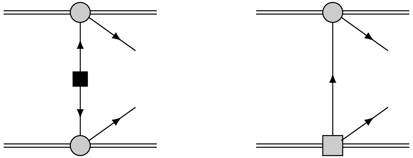
$ 0\nu\beta\beta $ -decay half-lives, following that of Ref. [19], and a brief introduction of its derivation is given in the appendices. We simultaneously consider two types of contributions: one arising from two SM vertices, and the other from one SM vertex combined with one BSM vertex, as shown in Fig. 1. The contribution of two high-dimensional operators is of the order$ {\cal{O}}(v^6/\Lambda^6) $ , and hence, it can be neglected compared to other contributions. Since$ C^{(6)}_{VL,VR} = {\cal{O}}(v^3/\Lambda^3) $ , where$ v = 246 $ GeV is the scalar field vacuum expectation value and Λ is the energy scale of the new physics. The terms associated with nucleon recoil momentum are neglected. For two SM vertices, we consider only the contribution of two outgoing s-wave electrons. For terms involving high-dimensional LEFT operators, only cases with less than or equal to one p-wave outgoing electron are considered. For the wave function of these emitted electrons, the approximation of no finite de-Broglie wavelength correction [19] (see also Appendices) is used to separate the phase-space factor and nuclear matrix element. Under the aforementioned approximation, the half-life of neutrinoless double beta decay can be expressed as (by sorting the decay width in Appendix C according to the Wilson coefficients):
Figure 1. Feynman diagrams for current study. Double lines and single lines represent nucleon and lepton fields, respectively. The filled gray circles and squares are the effective four fermion interaction vertices for the SM and new physics, respectively. The black square represents the insertion of the Majorana neutrino mass.
$ \begin{aligned}[b] \left[T^{0\nu}_{1/2}\right]^{-1}=\;&\frac{\Gamma^{0\nu}}{\ln2} =\Bigg\{C_{mm}\frac{\left|m_{\beta\beta}\right|^2}{m^2_e}-C_{m\lambda} {\rm Re}\left[\frac{m_{\beta\beta}}{m_e}\left(\frac{C_{VR}^{(6)}}{2V_{ud}}\right)^*\right]\\&-C_{m\eta}{\rm Re}\left[\frac{m_{\beta\beta}}{m_e} \left(\frac{C^{(6)}_{VL}}{2V_{ud}}\right)^*\right]+C_{\lambda\lambda}\left|\frac{C^{(6)}_{VR}}{2V_{ud}}\right|^2\\ &+C_{\eta\eta}\left|\frac{C_{VL}^{(6)}}{2V_{ud}}\right|^2+C_{\lambda\eta}{\rm Re}\left[\frac{C_{VL}^{(6)}}{2V_{ud}}\left(\frac{C_{VR}^{(6)}}{2V_{ud}}\right)^*\right]\Bigg\}, \end{aligned} $
(17) where
$ m_{\beta\beta} $ is the effective Majorana neutrino mass, which is defined as$ \begin{aligned} m_{\beta\beta} \equiv \sum_{i=1}^{3} U_{ei}^2 \, m_i, \end{aligned} $
(18) where
$ m_i $ represents the light neutrino masses and$ U_{ei} $ denotes the mixing matrix elements connecting the electron flavor to the i-th mass eigenstate.The coefficients
$ C's $ as functions of NMEs and phase space factors are defined as$ \begin{aligned}[b] C_{mm}=&G_{01}M^2_\nu ,\\ C_{m\lambda}=&C_{m\lambda\omega}+ C_{m\lambda q}\\ =&-G_{03}M_\nu M_{\omega R}+G_{04}M_\nu M_{qR},\\ C_{m\eta}=&C_{m\eta \omega}+C_{m\eta q}+C_{m\eta P}+C_{m\eta R}\\ =&G_{03}M_\nu M_{\omega L}-G_{04} M_\nu M_{qL} -G_{05}M_\nu M_P+ G_{06}M_\nu M_R,\\ C_{\lambda\lambda}=&C_{\lambda\lambda\omega}+C_{\lambda\lambda q }+C_{\lambda\lambda \omega q }\\ =&G_{02}M^2_{\omega R}+G_{011}M^2_{qR} + G_{010} M_{\omega R}M_{qR},\\ C_{\eta\eta}=&C_{\eta\eta\omega}+C_{\eta\eta q}+C_{\eta\eta\omega q}+C_{\eta\eta P}+C_{\eta\eta R}+C_{\eta\eta PR}\\ =&G_{02} M^2_{\omega L}+G_{011} M^2_{qL} + G_{010} M_{\omega L}M_{qL}\\&+ G_{08} M^2_P + G_{09} M^2_R - G_{07} M_P M_R , \\C_{\lambda\eta}=&C_{\lambda\eta \omega}+C_{\lambda\eta q}+C_{\lambda\eta \omega q}\end{aligned} $
$ \begin{aligned}[b] =&-2G_{02}M_{\omega L}M_{\omega R} -2 G_{011} M_{qL} M_{qR} \\&- G_{010} \left(M_{\omega L}M_{qR}+M_{\omega R}M_{qL}\right). \end{aligned} $
(19) Using these definitions, we can compare the expression of the decay width to that provided in various studies [19, 20, 28, 48] for the LRSM. By substituting Eq. (10), we obtain Eq. (33) in Ref. [28] with
$ \langle\lambda\rangle=\left|C_{VR}^{(6)}/(2V_{ud})\right|= \lambda \left|TU^{-1}\right|_{ee} $ and$ \langle\eta\rangle=-\left|C_{VL}^{(6)}/(2V_{ud})\right|=\eta \left|TU^{-1}\right|_{ee} $ . Up to this step, we have proven the equivalence between the EFT description and a model dependent description of$ 0\nu\beta\beta $ -decay for the LRSM from [19]. In this sense, in addition to the traditional model dependent description of$ 0\nu\beta\beta $ -decay, the SMEFT and LEFT provide very good tools for effectively connecting the different energy scales with renormalization groups.By rearranging the so-called master formula for the half-life of
$ 0\nu\beta\beta $ -decay in Ref. [15] in a form similar to Eq. (17), we obtain$ \begin{aligned}[b] C'_{mm}=&G_{01}M^2_\nu,\\ C'_{m\lambda}=&C'_{m\lambda \omega}+C'_{m\lambda q}\\ =&-G_{03}M_\nu M'_{\omega R}+G_{04}M_\nu M'_{q R}, \\ C'_{m\eta}=&C'_{m\eta\omega}+C'_{m\eta q}+C'_{m\eta R}\\ =&G_{03}M_\nu M'_{\omega L}-G_{04}M_\nu M'_{q L}+G_{06}M_\nu M'_R,\\ C'_{\lambda\lambda}=&C'_{\lambda\lambda\omega}+C'_{\lambda\lambda q} +C'_{\lambda\lambda\omega q}\\ =&G_{02}\left(M'_{\omega R}\right)^2+\frac{1}{9}\left(G_{02}+G_{03}+3G_{04} \right)\left(M'_{qR}\right)^2\\&-\frac{2}{3}\left(G_{02}+G_{03}\right)M'_{\omega R}M'_{qR},\\ C'_{\eta\eta}=&C'_{\eta\eta\omega}+C'_{\eta\eta q}+C'_{\eta\eta\omega q}+C'_{\eta\eta R}\\ =&G_{02}\left(M'_{\omega L}\right)^2+\frac{1}{9}\left(G_{02}+G_{03}+3G_{04} \right)\left(M'_{qL}\right)^2\\&-\frac{2}{3}\left(G_{02}+G_{03}\right)M'_{\omega L}M'_{qL}+G_{09}\left(M'_R\right)^2,\\ C'_{\lambda\eta}=&C'_{\lambda\eta\omega}+C'_{\lambda\eta q}+C'_{\lambda\eta\omega q}\\ =&-2G_{02}M'_{\omega L}M'_{\omega R}-\frac{2}{9}\left(G_{02}+G_{03}+3G_{04} \right)M'_{qL}M'_{qR}\\&+\frac{2}{3}\left(G_{02}+G_{03}\right)\left(M'_{\omega L}M'_{q R}+M'_{\omega R}M'_{q L}\right). \end{aligned} $
(20) A detailed term-by-term comparison between Eq. (19) and the master formula in Eq. (20) shows that the phase space factors and NMEs in the two formalisms exhibit an almost one-to-one correspondence. The phase space factors used in this comparison are summarized in Table 1. Although most phase space factors coincide precisely, a few terms differ slightly in their form. Specifically, the coefficient
$ G_{011} $ in front of the q-type NMEs in Eq. (19) is replaced with$ (G_{02} + G_{03} + 3G_{04})/9 $ in Eq. (20), and the interference term involving q and ω, originally accompanied by$ G_{010} $ , corresponds to$ (G_{02} + G_{03})/3 $ in the master formula. These are obtained by considering the numerical wave functions of p-wave electrons [25]. Despite these differences, a numerical comparison confirms that the deviations remain below 5%, rendering the two prescriptions effectively equivalent for practical purposes [25].76Ge 82Se 130Te 136Xe $Q_{\beta\beta }\ /{\rm{MeV}}$ 2.039 2.995 2.527 2.458 $10^{14}G_{01}$ 0.237 1.018 1.425 1.462 $10^{14}G_{02}$ 0.391 3.529 3.761 3.679 $10^{15}G_{03}$ 1.305 6.913 8.967 9.047 $10^{14}G_{04}$ 0.185 0.873 1.205 1.231 $10^{13}G_{05}$ 0.566 2.004 3.790 4.015 $10^{12}G_{06}$ 0.531 1.733 2.227 2.275 $10^{10}G_{07}$ 0.270 1.163 1.755 1.812 $10^{11}G_{08}$ 0.149 0.708 1.549 1.657 $10^{10}G_{09}$ 1.223 4.779 4.972 4.956 $10^{14}G_{010}$ 0.177 1.443 1.636 1.615 $10^{14}G_{011}$ 0.122 0.788 0.987 0.991 Table 1. Phase space factors in units of
$ {\rm{yr}}^{-1} $ obtained from Ref. [28]. The first row shows the$ Q_{\beta\beta} $ values for the different isotopes, where$ Q_{\beta\beta} = M_i - M_f - 2m_e $ .Therefore, the principal difference between the two approaches lies in the choice of nuclear matrix elements whose forms are presented in Appendix B, which we examine in detail in the following discussion.
-
In this work, we adopt the S-matrix theory to derive
$ 0\nu\beta\beta $ -decay half-lives, following that of Ref. [19], and a brief introduction of its derivation is given in the appendices. The contribution of two high-dimensional operators is at the order of$ {\cal{O}}(v^6/\Lambda^6) $ , hence it can be neglected compared to other contributions. Since$ C^{(6)}_{VL,VR} ={\cal{O}}(v^3/\Lambda^3) $ , where$ v = 246 $ GeV is the scalar field vacuum expectation value and Λ is the energy scale of new physics. The terms associated with nucleon recoil momentum are neglected. For two SM vertices, we consider only the contribution of two outgoing s-wave electrons. For terms involving high-dimensional LEFT operators, only cases with less than or equal one p-wave outgoing electron is considered. For wave function of these emitted electrons, the approximation of no finite de-Broglie wavelength correction (noFBWC) [19] (see also Appendices) is used in order to separate the phase-space factor and the nuclear matrix element. Under the aforementioned approximation, the half-life of neutrinoless double beta decay can be expressed as (By sorting the decay width in Appendix C according to the Wilson coefficients):$ \begin{aligned}[b] \left[T^{0\nu}_{1/2}\right]^{-1}=\;&\frac{\Gamma^{0\nu}}{\ln2} =\Bigg\{C_{mm}\frac{\left|m_{\beta\beta}\right|^2}{m^2_e}-C_{m\lambda} Re\left[\frac{m_{\beta\beta}}{m_e}\left(\frac{C_{VR}^{(6)}}{2V_{ud}}\right)^*\right]\\&-C_{m\eta}Re\left[\frac{m_{\beta\beta}}{m_e} \left(\frac{C^{(6)}_{VL}}{2V_{ud}}\right)^*\right]+C_{\lambda\lambda}\left|\frac{C^{(6)}_{VR}}{2V_{ud}}\right|^2\\ &+C_{\eta\eta}\left|\frac{C_{VL}^{(6)}}{2V_{ud}}\right|^2+C_{\lambda\eta}Re\left[\frac{C_{VL}^{(6)}}{2V_{ud}}\left(\frac{C_{VR}^{(6)}}{2V_{ud}}\right)^*\right]\Bigg\}, \end{aligned} $

(17) where
$ m_{\beta\beta} $ is the effective Majorana neutrino mass, defined as:$ \begin{aligned} m_{\beta\beta} \equiv \sum_{i=1}^{3} U_{ei}^2 \, m_i, \end{aligned} $

(18) with
$ m_i $ being the light neutrino masses and$ U_{ei} $ the mixing matrix elements connecting the electron flavor to the i-th mass eigenstate.The coefficients
$ C's $ as functions of NMEs and phase space factors are defined as:$ \begin{aligned}[b] C_{mm}=&G_{01}M^2_\nu ,\\ C_{m\lambda}=&C_{m\lambda\omega}+ C_{m\lambda q}\\ =&-G_{03}M_\nu M_{\omega R}+G_{04}M_\nu M_{qR},\\ C_{m\eta}=&C_{m\eta \omega}+C_{m\eta q}+C_{m\eta P}+C_{m\eta R}\\ =&G_{03}M_\nu M_{\omega L}-G_{04} M_\nu M_{qL} -G_{05}M_\nu M_P+ G_{06}M_\nu M_R,\\ C_{\lambda\lambda}=&C_{\lambda\lambda\omega}+C_{\lambda\lambda q }+C_{\lambda\lambda \omega q }\\ =&G_{02}M^2_{\omega R}+G_{011}M^2_{qR} + G_{010} M_{\omega R}M_{qR},\\ C_{\eta\eta}=&C_{\eta\eta\omega}+C_{\eta\eta q}+C_{\eta\eta\omega q}+C_{\eta\eta P}+C_{\eta\eta R}+C_{\eta\eta PR}\\ =&G_{02} M^2_{\omega L}+G_{011} M^2_{qL} + G_{010} M_{\omega L}M_{qL}\\&+ G_{08} M^2_P + G_{09} M^2_R - G_{07} M_P M_R ,\\ C_{\lambda\eta}=&C_{\lambda\eta \omega}+C_{\lambda\eta q}+C_{\lambda\eta \omega q}\\ =&-2G_{02}M_{\omega L}M_{\omega R} -2 G_{011} M_{qL} M_{qR} \\&- G_{010} \left(M_{\omega L}M_{qR}+M_{\omega R}M_{qL}\right). \end{aligned} $

(19) With these definitions, we could compare the expression of the decay width to that given in various literature [19, 28, 48, 49] for LRSM. By substituting eq.(10), we obtain the eq.(33) in Ref. [28] with
$ \langle\lambda\rangle=\left|C_{VR}^{(6)}/(2V_{ud})\right|= \lambda \left|TU^{-1}\right|_{ee} $ and$ \langle\eta\rangle=-\left|C_{VL}^{(6)}/(2V_{ud})\right|=\eta \left|TU^{-1}\right|_{ee} $ . Till this step, we have proven the equivalence between EFT description and a model dependent description of$ 0\nu\beta\beta $ -decay for the LRSM from [19]. In this sense, in addition to traditional model dependent description of$ 0\nu\beta\beta $ -decay, SMEFT and LEFT provide very good tools which could well connect the different energy scales with renormalization groups.By rearranging the so-called master formula for the half-life of
$ 0\nu\beta\beta $ -decay in Ref. [15] in a form similar to Eq.(17), we obtain:$ \begin{aligned}[b] C'_{mm}=&G_{01}M^2_\nu,\\ C'_{m\lambda}=&C'_{m\lambda \omega}+C'_{m\lambda q}\\ =&-G_{03}M_\nu M'_{\omega R}+G_{04}M_\nu M'_{q R}, \\ C'_{m\eta}=&C'_{m\eta\omega}+C'_{m\eta q}+C'_{m\eta R}\\ =&G_{03}M_\nu M'_{\omega L}-G_{04}M_\nu M'_{q L}+G_{06}M_\nu M'_R,\\ C'_{\lambda\lambda}=&C'_{\lambda\lambda\omega}+C'_{\lambda\lambda q} +C'_{\lambda\lambda\omega q}\\ =&G_{02}\left(M'_{\omega R}\right)^2+\frac{1}{9}\left(G_{02}+G_{03}+3G_{04} \right)\left(M'_{qR}\right)^2\\&-\frac{2}{3}\left(G_{02}+G_{03}\right)M'_{\omega R}M'_{qR},\\ C'_{\eta\eta}=&C'_{\eta\eta\omega}+C'_{\eta\eta q}+C'_{\eta\eta\omega q}+C'_{\eta\eta R}\\ =&G_{02}\left(M'_{\omega L}\right)^2+\frac{1}{9}\left(G_{02}+G_{03}+3G_{04} \right)\left(M'_{qL}\right)^2\\&-\frac{2}{3}\left(G_{02}+G_{03}\right)M'_{\omega L}M'_{qL}+G_{09}\left(M'_R\right)^2,\\ C'_{\lambda\eta}=&C'_{\lambda\eta\omega}+C'_{\lambda\eta q}+C'_{\lambda\eta\omega q}\\ =&-2G_{02}M'_{\omega L}M'_{\omega R}-\frac{2}{9}\left(G_{02}+G_{03}+3G_{04} \right)M'_{qL}M'_{qR}\\&+\frac{2}{3}\left(G_{02}+G_{03}\right)\left(M'_{\omega L}M'_{q R}+M'_{\omega R}M'_{q L}\right). \end{aligned} $

(20) A detailed term-by-term comparison between eq.(19) and the master formula in eq.(20) shows that the phase space factors and NMEs in the two formalisms exhibit an almost one-to-one correspondence. While the majority of phase space factors coincide exactly, a few terms differ slightly in their form. Specifically, the coefficient
$ G_{011} $ in front of the q-type NMEs in eq.(19) is replaced by$ (G_{02} + G_{03} + 3G_{04})/9 $ in eq.(20), and the interference term involving q and ω, originally accompanied by$ G_{010} $ , corresponds to$ (G_{02} + G_{03})/3 $ in the master formula. These are obtained by considering numerical wave functions of p-wave electrons [25]. Despite these differences, a numerical comparison confirms that the deviations remain below 5%, rendering the two prescriptions effectively equivalent for practical purposes [25].Therefore, the principal difference between the two approaches lies in the choice of nuclear matrix elements whose forms are given in Appendix.B, we will examine in detail in the following discussion.
-
In this study, we adopt the S-matrix theory to derive
$ 0\nu\beta\beta $ -decay half-lives, following that of Ref. [19], and a brief introduction of its derivation is given in the appendices. We simultaneously consider two types of contributions: one arising from two SM vertices, and the other from one SM vertex combined with one BSM vertex, as shown in Fig. 1. The contribution of two high-dimensional operators is of the order$ {\cal{O}}(v^6/\Lambda^6) $ , and hence, it can be neglected compared to other contributions. Since$ C^{(6)}_{VL,VR} = {\cal{O}}(v^3/\Lambda^3) $ , where$ v = 246 $ GeV is the scalar field vacuum expectation value and Λ is the energy scale of the new physics. The terms associated with nucleon recoil momentum are neglected. For two SM vertices, we consider only the contribution of two outgoing s-wave electrons. For terms involving high-dimensional LEFT operators, only cases with less than or equal to one p-wave outgoing electron are considered. For the wave function of these emitted electrons, the approximation of no finite de-Broglie wavelength correction [19] (see also Appendices) is used to separate the phase-space factor and nuclear matrix element. Under the aforementioned approximation, the half-life of neutrinoless double beta decay can be expressed as (by sorting the decay width in Appendix C according to the Wilson coefficients):
Figure 1. Feynman diagrams for current study. Double lines and single lines represent nucleon and lepton fields, respectively. The filled gray circles and squares are the effective four fermion interaction vertices for the SM and new physics, respectively. The black square represents the insertion of the Majorana neutrino mass.
$ \begin{aligned}[b] \left[T^{0\nu}_{1/2}\right]^{-1}=\;&\frac{\Gamma^{0\nu}}{\ln2} =\Bigg\{C_{mm}\frac{\left|m_{\beta\beta}\right|^2}{m^2_e}-C_{m\lambda} {\rm Re}\left[\frac{m_{\beta\beta}}{m_e}\left(\frac{C_{VR}^{(6)}}{2V_{ud}}\right)^*\right]\\&-C_{m\eta}{\rm Re}\left[\frac{m_{\beta\beta}}{m_e} \left(\frac{C^{(6)}_{VL}}{2V_{ud}}\right)^*\right]+C_{\lambda\lambda}\left|\frac{C^{(6)}_{VR}}{2V_{ud}}\right|^2\\ &+C_{\eta\eta}\left|\frac{C_{VL}^{(6)}}{2V_{ud}}\right|^2+C_{\lambda\eta}{\rm Re}\left[\frac{C_{VL}^{(6)}}{2V_{ud}}\left(\frac{C_{VR}^{(6)}}{2V_{ud}}\right)^*\right]\Bigg\}, \end{aligned} $
(17) where
$ m_{\beta\beta} $ is the effective Majorana neutrino mass, which is defined as$ \begin{aligned} m_{\beta\beta} \equiv \sum_{i=1}^{3} U_{ei}^2 \, m_i, \end{aligned} $
(18) where
$ m_i $ represents the light neutrino masses and$ U_{ei} $ denotes the mixing matrix elements connecting the electron flavor to the i-th mass eigenstate.The coefficients
$ C's $ as functions of NMEs and phase space factors are defined as$ \begin{aligned}[b] C_{mm}=&G_{01}M^2_\nu ,\\ C_{m\lambda}=&C_{m\lambda\omega}+ C_{m\lambda q}\\ =&-G_{03}M_\nu M_{\omega R}+G_{04}M_\nu M_{qR},\\ C_{m\eta}=&C_{m\eta \omega}+C_{m\eta q}+C_{m\eta P}+C_{m\eta R}\\ =&G_{03}M_\nu M_{\omega L}-G_{04} M_\nu M_{qL} -G_{05}M_\nu M_P+ G_{06}M_\nu M_R,\\ C_{\lambda\lambda}=&C_{\lambda\lambda\omega}+C_{\lambda\lambda q }+C_{\lambda\lambda \omega q }\\ =&G_{02}M^2_{\omega R}+G_{011}M^2_{qR} + G_{010} M_{\omega R}M_{qR},\\ C_{\eta\eta}=&C_{\eta\eta\omega}+C_{\eta\eta q}+C_{\eta\eta\omega q}+C_{\eta\eta P}+C_{\eta\eta R}+C_{\eta\eta PR}\\ =&G_{02} M^2_{\omega L}+G_{011} M^2_{qL} + G_{010} M_{\omega L}M_{qL}\\&+ G_{08} M^2_P + G_{09} M^2_R - G_{07} M_P M_R , \\C_{\lambda\eta}=&C_{\lambda\eta \omega}+C_{\lambda\eta q}+C_{\lambda\eta \omega q}\end{aligned} $
$ \begin{aligned}[b] =&-2G_{02}M_{\omega L}M_{\omega R} -2 G_{011} M_{qL} M_{qR} \\&- G_{010} \left(M_{\omega L}M_{qR}+M_{\omega R}M_{qL}\right). \end{aligned} $
(19) Using these definitions, we can compare the expression of the decay width to that provided in various studies [19, 20, 28, 48] for the LRSM. By substituting Eq. (10), we obtain Eq. (33) in Ref. [28] with
$ \langle\lambda\rangle=\left|C_{VR}^{(6)}/(2V_{ud})\right|= \lambda \left|TU^{-1}\right|_{ee} $ and$ \langle\eta\rangle=-\left|C_{VL}^{(6)}/(2V_{ud})\right|=\eta \left|TU^{-1}\right|_{ee} $ . Up to this step, we have proven the equivalence between the EFT description and a model dependent description of$ 0\nu\beta\beta $ -decay for the LRSM from [19]. In this sense, in addition to the traditional model dependent description of$ 0\nu\beta\beta $ -decay, the SMEFT and LEFT provide very good tools for effectively connecting the different energy scales with renormalization groups.By rearranging the so-called master formula for the half-life of
$ 0\nu\beta\beta $ -decay in Ref. [15] in a form similar to Eq. (17), we obtain$ \begin{aligned}[b] C'_{mm}=&G_{01}M^2_\nu,\\ C'_{m\lambda}=&C'_{m\lambda \omega}+C'_{m\lambda q}\\ =&-G_{03}M_\nu M'_{\omega R}+G_{04}M_\nu M'_{q R}, \\ C'_{m\eta}=&C'_{m\eta\omega}+C'_{m\eta q}+C'_{m\eta R}\\ =&G_{03}M_\nu M'_{\omega L}-G_{04}M_\nu M'_{q L}+G_{06}M_\nu M'_R,\\ C'_{\lambda\lambda}=&C'_{\lambda\lambda\omega}+C'_{\lambda\lambda q} +C'_{\lambda\lambda\omega q}\\ =&G_{02}\left(M'_{\omega R}\right)^2+\frac{1}{9}\left(G_{02}+G_{03}+3G_{04} \right)\left(M'_{qR}\right)^2\\&-\frac{2}{3}\left(G_{02}+G_{03}\right)M'_{\omega R}M'_{qR},\\ C'_{\eta\eta}=&C'_{\eta\eta\omega}+C'_{\eta\eta q}+C'_{\eta\eta\omega q}+C'_{\eta\eta R}\\ =&G_{02}\left(M'_{\omega L}\right)^2+\frac{1}{9}\left(G_{02}+G_{03}+3G_{04} \right)\left(M'_{qL}\right)^2\\&-\frac{2}{3}\left(G_{02}+G_{03}\right)M'_{\omega L}M'_{qL}+G_{09}\left(M'_R\right)^2,\\ C'_{\lambda\eta}=&C'_{\lambda\eta\omega}+C'_{\lambda\eta q}+C'_{\lambda\eta\omega q}\\ =&-2G_{02}M'_{\omega L}M'_{\omega R}-\frac{2}{9}\left(G_{02}+G_{03}+3G_{04} \right)M'_{qL}M'_{qR}\\&+\frac{2}{3}\left(G_{02}+G_{03}\right)\left(M'_{\omega L}M'_{q R}+M'_{\omega R}M'_{q L}\right). \end{aligned} $
(20) A detailed term-by-term comparison between Eq. (19) and the master formula in Eq. (20) shows that the phase space factors and NMEs in the two formalisms exhibit an almost one-to-one correspondence. The phase space factors used in this comparison are summarized in Table 1. Although most phase space factors coincide precisely, a few terms differ slightly in their form. Specifically, the coefficient
$ G_{011} $ in front of the q-type NMEs in Eq. (19) is replaced with$ (G_{02} + G_{03} + 3G_{04})/9 $ in Eq. (20), and the interference term involving q and ω, originally accompanied by$ G_{010} $ , corresponds to$ (G_{02} + G_{03})/3 $ in the master formula. These are obtained by considering the numerical wave functions of p-wave electrons [25]. Despite these differences, a numerical comparison confirms that the deviations remain below 5%, rendering the two prescriptions effectively equivalent for practical purposes [25].76Ge 82Se 130Te 136Xe $Q_{\beta\beta }\ /{\rm{MeV}}$ 2.039 2.995 2.527 2.458 $10^{14}G_{01}$ 0.237 1.018 1.425 1.462 $10^{14}G_{02}$ 0.391 3.529 3.761 3.679 $10^{15}G_{03}$ 1.305 6.913 8.967 9.047 $10^{14}G_{04}$ 0.185 0.873 1.205 1.231 $10^{13}G_{05}$ 0.566 2.004 3.790 4.015 $10^{12}G_{06}$ 0.531 1.733 2.227 2.275 $10^{10}G_{07}$ 0.270 1.163 1.755 1.812 $10^{11}G_{08}$ 0.149 0.708 1.549 1.657 $10^{10}G_{09}$ 1.223 4.779 4.972 4.956 $10^{14}G_{010}$ 0.177 1.443 1.636 1.615 $10^{14}G_{011}$ 0.122 0.788 0.987 0.991 Table 1. Phase space factors in units of
$ {\rm{yr}}^{-1} $ obtained from Ref. [28]. The first row shows the$ Q_{\beta\beta} $ values for the different isotopes, where$ Q_{\beta\beta} = M_i - M_f - 2m_e $ .Therefore, the principal difference between the two approaches lies in the choice of nuclear matrix elements whose forms are presented in Appendix B, which we examine in detail in the following discussion.
-
The calculation of NMEs relies on specific nuclear many-body models, and the results obtained using different methods often vary significantly. This is observed for the NMEs of the mass mechanism. A large deviation is evident for different calculations [49, 50]. However, the NMEs for other mechanisms are relatively limited, and until recently, calculations have included all LO components for the λ mechanism [51, 52].
In this work, we obtain the NMEs mainly from two previous calculations: the first calculations [52] using the QRPA with the realistic NN force CD-Bonn [53], where one adopts a model space with eight major shells (N=0−7). In addition, short-range correlations with CD-Bonn parametrization are incorporated into our calculations [54]. We adopt a bare axial vector coupling constant
$ g_A=1.27 $ , and the parameters are determined as in [55], the only difference being that in the current study, the BCS overlap factors in [52] are included and one finds that this adjustment changes the final results slightly, except for the semi-magic nucleus 136Xe. The second calculation is obtained from the large scale nuclear shell model (LSSM) calculations [51], where for each nuclei, two different Hamiltonians are used (for the lighter nuclei, 76Ge and 82Se,$ jun45 $ and$ jj44b $ , respectively, and for the heavier nuclei 130Te and 136Xe,$ jj55a $ and$ GCN50:82 $ ). These two calculations are used to illustrate the uncertainties from various aspects.In Eq. (19), we actually have 7 different terms of NMEs, within which one term (
$ M_{\nu} $ ) is related to the dim-3 LEFT operator$ m_{\beta\beta} $ , two terms ($ M_{\omega R} $ and$ M_{q R} $ ) are related tothe dim-6 LEFT operator$ C_{VR}^{(6)} $ , and four terms ($ M_{\omega L} $ ,$ M_{q L} $ ,$ M_{R} $ , and$ M_{P} $ ) are related to the dim-6 LEFT operator$ C_{VL}^{(6)} $ . Each term except for$ M_{P} $ then consists of different parts, namely the Fermi, GT, and tensor parts ($ M_R $ has only the GT and tensor parts). In addition, different parts may consist of different components, as explicitly detailed in Appendix B.Of these different terms, some are closely related, that is,
$ M_{\omega L} $ and$ M_{\omega R} $ or$ M_{q L} $ and$ M_{q R} $ . They only differ from their counterparts in the sign for the components related to the vector current and weak-magnetism current.Detailed lists of the values for these NMEs are presented in Tables 2 and 3, where two Hamiltonians are adopted for the LSSM calculations, as stated above. We start with the mass mechanism. For these NMEs, we numerous calculations and abundant discussions on the uncertainties for various many-body methods have been provided [56−58], and this is not the main topic of the current study. As detailed discussions of these NMEs are presented in Ref. [51], we focus on discussing the difference between these two calculations in this work. For the QRPA results, we observe a minor change by including the BCS overlap factors, and we find that this barely changes the results except for the case of 136Xe.
NMEs 76Ge 82Se 130Te 136Xe QRPA jun45 jj44b QRPA jun45 jj44b QRPA jj55a GCN50:82 QRPA jj55a GCN50:82 $M_F$ −1.314 −0.665 −0.602 −1.180 −0.624 −0.523 −1.155 −0.668 −0.702 −0.345 −0.574 −0.568 $M^{AA}_{GT}$ 5.139 3.584 3.278 4.387 3.360 2.860 3.988 3.147 3.180 1.493 2.648 2.549 $M^{AP}_{GT}$ −1.961 −1.090 −0.960 −1.708 −1.021 −0.834 −1.681 −0.979 −1.034 −0.597 −0.820 −0.829 $M^{PP}_{GT}$ 0.671 0.344 0.300 0.586 0.321 0.261 0.594 0.313 0.335 0.207 0.260 0.268 $M^{MM}_{GT}$ 0.828 0.247 0.215 0.717 0.229 0.188 0.733 0.227 0.244 0.250 0.188 0.194 $M_{GT}$ 4.362 2.991 2.751 3.710 2.802 2.404 3.355 2.622 2.632 1.258 2.205 2.108 $M^{AA}_{T}$ −1.833 −0.086 −0.052 −1.704 −0.084 −0.062 −2.262 −0.059 −0.024 −0.704 −0.053 −0.005 $M^{AP}_{T}$ −0.809 −0.013 −0.004 −0.749 −0.014 −0.012 −0.965 0.008 0.015 −0.294 0.002 0.014 $M^{PP}_{T}$ 0.296 0.002 −0.001 0.272 0.003 0.003 0.342 −0.006 −0.007 0.103 −0.003 −0.006 $M^{MM}_{T}$ −0.121 −0.001 0.000 −0.110 −0.001 −0.002 −0.134 0.003 0.003 −0.040 0.001 0.002 $M_{T}$ −0.588 −0.012 −0.005 −0.546 −0.012 −0.010 −0.706 0.004 0.011 −0.216 0.000 0.009 Table 2.
$ 0\nu\beta\beta $ –decay NMEs for 76Ge, 82Se, 130Te, and 136Xe. The table shows all components of the NMEs defined by Eq. (B6), including those required for the master formula in Ref. [15]. Results are presented for QRPA and shell model calculations with two different Hamiltonians. All NMEs are evaluated at$ g_A = 1 $ . For consistent comparison and summation, the MM terms are rescaled by$ 1/g_A^2 $ with$ g_A=1.27 $ .NMEs 76Ge 82Se 130Te 136Xe QRPA jun45 jj44b QRPA jun45 jj44b QRPA jj55a GCN50:82 QRPA jj55a GCN50:82 $ M_{\omega F}$ −1.290 −0.637 −0.576 −1.156 −0.597 −0.500 −1.152 −0.637 −0.669 −0.341 −0.545 −0.540 $ M^{AA}_{\omega GT}$ 5.036 3.276 2.980 4.339 3.073 2.596 4.025 2.883 2.931 1.450 2.427 2.351 $ M^{AP}_{\omega GT}$ −1.929 −1.044 −0.919 −1.684 −0.978 −0.798 −1.665 −0.939 −0.993 −0.580 −0.786 −0.795 $ M^{PP}_{\omega GT}$ 0.661 0.333 0.290 0.577 0.310 0.252 0.587 0.303 0.324 0.201 0.252 0.259 $ M^{MM}_{\omega GT}$ 0.814 0.239 0.208 0.707 0.221 0.181 0.723 0.220 0.236 0.244 0.182 0.188 $ M_{\omega LGT}$ 4.272 2.713 2.480 3.670 2.542 2.162 3.395 2.383 2.408 1.223 2.006 1.932 $ M_{\omega RGT}$ 3.264 2.417 2.222 2.794 2.268 1.938 2.499 2.111 2.116 0.919 1.780 1.698 $ M^{AP}_{\omega T}$ −0.785 −0.012 −0.003 −0.726 −0.013 −0.011 −0.926 0.009 0.015 −0.283 0.003 0.014 $ M^{PP}_{\omega T}$ 0.287 0.002 −0.001 0.265 0.003 0.003 0.330 −0.006 −0.007 0.100 −0.003 −0.006 $ M^{MM}_{\omega T}$ −0.191 −0.001 0.000 −0.174 −0.001 −0.002 −0.210 0.003 0.003 −0.064 0.001 0.002 $ M_{\omega LT}$ −0.616 −0.011 −0.004 −0.569 −0.011 −0.010 −0.726 0.006 0.010 −0.222 0.001 0.009 $ M_{\omega RGT}$ −0.380 −0.009 −0.004 −0.353 −0.009 −0.007 −0.466 0.000 0.006 −0.144 −0.001 0.007 $ M_{qF}$ −0.797 −0.379 −0.352 −0.734 −0.360 −0.303 −0.683 −0.408 −0.418 −0.195 −0.358 −0.342 $ M^{AA}_{qGT}$ 1.266 1.070 0.994 1.062 1.005 0.868 0.891 0.927 0.917 0.367 0.783 0.736 $ M^{AP}_{qGT}$ 2.499 1.614 1.439 2.173 1.524 1.247 2.024 1.422 1.475 0.760 1.202 1.188 $ M^{PP}_{qGT}$ −1.104 −0.648 −0.569 −0.967 −0.610 −0.493 −0.945 −0.577 −0.609 −0.345 −0.485 −0.489 $ M^{MM}_{qGT}$ −1.959 −0.625 −0.545 −1.707 −0.582 −0.475 −1.734 −0.569 −0.608 −0.607 −0.473 −0.485 $ M_{qLGT}$ 1.447 1.412 1.526 1.210 1.338 1.328 0.895 1.203 1.406 0.406 1.027 1.134 $ M_{qRGT}$ 3.875 2.661 2.202 3.327 2.501 1.917 3.044 2.342 2.160 1.159 1.973 1.736 $ M^{AA}_{qT}$ 2.874 0.112 0.066 2.660 0.110 0.084 3.456 0.062 0.018 1.070 0.062 −0.004 $ M^{AP}_{qT}$ −1.534 −0.008 0.002 −1.406 −0.012 −0.016 −1.730 0.036 0.036 −0.522 0.014 0.030 $ M^{PP}_{qT}$ 0.458 −0.000 −0.002 0.416 0.002 0.006 0.484 −0.014 −0.010 0.144 −0.004 −0.006 $ M^{MM}_{qT}$ 0.178 −0.000 −0.000 0.158 −0.000 0.002 0.174 −0.002 −0.002 0.052 −0.000 −0.002 $ M_{qL,T}$ 1.908 0.104 0.066 1.768 0.100 0.076 2.318 0.082 0.042 0.724 0.072 0.018 $ M_{qR,T}$ 1.688 0.104 0.066 1.572 0.100 0.072 2.102 0.086 0.046 0.660 0.072 0.022 $ M_{RGT}$ 9.292 4.235 3.713 8.250 4.037 3.314 9.846 4.686 5.048 3.393 3.948 4.080 $ M_{RT}$ −2.281 0.014 0.004 −2.128 0.018 0.028 −2.983 −0.056 −0.056 −0.910 −0.014 −0.042 $ M_R$ 7.011 4.249 3.717 6.123 4.055 3.342 6.863 4.630 4.992 2.483 3.934 4.038 $ M_P$ −0.562 −0.431 −0.279 −0.521 −0.428 −0.152 −0.281 −0.498 −0.425 −0.203 −0.289 −0.255 Table 3. NMEs for
$ 0\nu\beta\beta $ -decay mechanisms beyond the mass mechanism in 76Ge, 82Se, 130Te, and 136Xe. The same conventions and normalization as in Table 2 are used.We start with the results for
$ M_{\nu} $ (Table 2). At first glance, we observe a drastic suppression of NMEs for 136Xe, which has never been reported in spherical calculations through observation in deformed QRPA calculations [59]. As 136Xe is a semi-magic nucleus, the newly incorporated BCS overlap factor may be underestimated compared with GCM calculations with restored particle numbers. The difference between the two approaches is pronounced: for the GT part, the QRPA calculations are approximately 30% to 50% larger, except for 136Xe, as explained above. The magnitude of the QRPA calculation may originate from the lack of certain nuclear correlations, for example, an explicit account of nuclear deformation could reduce the NMEs and the deviation between the QRPA and LSSM calculations [59]. Another difference between the two approaches is the relative magnitude of the tensor part, which is more than 10% for QRPA but negligible for LSSM calculations. In contrast, for the Fermi part,$ M_F=-1/3M_{GT} $ was first observed for the QRPA in [55] with the restoration of isospin symmetry, which agrees with a naive analysis from the Fierz rearrangement, but for LSSM, such a ratio is slightly smaller in magnitude, by only$ -1/4 $ . This may originate from the heavily truncated model space, and similar suppression can be observed if this model space is adopted in QRPA calculations.As
$ M_{\omega} $ and$ M_{\nu} $ differ only in the energy denominator, the corresponding components are basically the same, and the deviation is within 5%, as is the difference between the two approaches. For the ω term, because of the different structures of the corresponding currents of the terms in Eq. (15) associated with$ C_{VL}^{(6)} $ and$ C_{VR}^{(6)} $ , the final NMEs are different, namely$ M_{\omega L} $ and$ M_{\omega R} $ , as defined previously.Whereas the ω term is basically the same as the mass term, the q terms behave quite differently in many respects, which is mostly because of the different angular momentum transfer of the neutrino propagators. Although the total angular momentum transfer is the same, one unit of orbital angular momentum is carried away by the p-wave electron, which dramatically changes the transition strength for similar operators, as we will observe later.
As discussed in [51], the q term differs from other terms in various aspects. In summary, for the GT part, a 1/3 factor in front of the AA component and enhancement from high transfer momenta together make the AP component the largest and the other components comparable. However, for the mass mechanism, deviations are observed for the two many-body calculations, mainly for the tensor part. The effect is more pronounced for q terms, because one finds from the QRPA calculations that they are comparable to the Fermi part or even GT part. Therefore, instead of a 10% correction, a 30% or 40% correction should be seriously considered.
As pointed out in Ref. [26], the R term dominates in the η mechanism. Although the weak-magnetism component of the nucleon current is considered to have an NLO effect in EFT and is thus expected to be suppressed, its contribution is significantly enhanced owing to the large value of
$ \mu_p - \mu_n $ . Under the current definition, QRPA calculations show that$ M_R $ — the NME corresponding to the R term — is approximately twice as large as those from other contributions. In contrast, the LSSM calculation yields a smaller NME, with the GT part being only half of the QRPA result and the tensor part almost negligible, which in the QRPA calculation serves to cancel out the GT contribution partially. As a result, a suppression of approximately 40% is observed in the LSSM, which indicates that precise predictions for the η mechanism depend strongly on the nuclear many-body method adopted.The importance of the P term was first proposed in [19]. However, various many-body calculations suggest that the corresponding NME is suppressed to approximately 1/10 of other NMEs. With these suppressed NMEs, the contribution from the P term can now be safely neglected for the η mechanism.
-
The calculation of NMEs relies on specific nuclear many-body models, and the results obtained using different methods often vary significantly. This is observed for the NMEs of mass mechanism. A large deviation is found for different calculations [50, 51]. However, the NMEs for other mechanisms are relatively limited, until recently, we have calculations which include all the LO components for λ mechanism [52, 53].
In this work, we take the NMEs mainly from two previous calculations: the first calculations [53] using the Quasi-Particle Random-Phase Approximation (QRPA) with the realistic NN force CD-Bonn [54] where one adopts a model space with eight major shells (N=0-7). Additionally, short-range correlations (SRC) with CD-Bonn parametrization are incorporated into our calculations [55]. We adopt a bare axial vector coupling constant
$ g_A=1.27 $ , and the parameters are determined as in [56], the only difference is that in current study, the BCS overlap factors in [53] is include and one finds that this adjustment changes the final results slightly except for semi-magic nucleus 136Xe. The second calculation is from the large scale nuclear shell model (LSSM) calculations [52], where for each nuclei, two different Hamiltonians are used (for the lighter nuclei, 76Ge and 82Se,$ jun45 $ and$ jj44b $ respectively, while for the heavier nuclei, 130Te and 136Xe,$ jj55a $ and$ GCN50:82 $ ). These two calculations are used to illustrate the uncertainties from various aspects.In eq.(19), we have actually 7 different terms of NMEs, within which, one term (
$ M_{\nu} $ ) is related to the Dim-3 LEFT operator$ m_{\beta\beta} $ , two terms ($ M_{\omega R} $ and$ M_{q R} $ ) are related to dim-6 LEFT operator$ C_{VR}^{(6)} $ and four terms ($ M_{\omega L} $ ,$ M_{q L} $ ,$ M_{R} $ and$ M_{P} $ ) related to dim-6 LEFT operator$ C_{VL}^{(6)} $ . Each term except$ M_{P} $ then consists of different parts, namely the Fermi, GT and Tensor parts ($ M_R $ has only GT and tensor parts). And different parts may consist of different components, this is given explicitly in Appendix B.Of these different terms, some are closely related, that is
$ M_{\omega L} $ and$ M_{\omega R} $ , or$ M_{q L} $ and$ M_{q R} $ . They just differ with their counterpart by the sign for the components related to the vector current and weak-magnetism current.A detailed list of the values for these NMEs are presented in Table 2 and 3, where for the LSSM calculations, as stated above, two Hamiltonians are adopted. We start with the mass mechanism, for these NMEs, we have plenty of calculations and abundant discussions on the uncertainties for various many-body methods [57−59], this is not the main topic of current study. Since there are detailed discussions of these NMEs in Ref. [52] for these two calculations respectively, in this work, we focus on the discussion of their difference. And for the QRPA results we have a minor change by including the BCS overlap factors and we find that this barely changes the results except for the case of 136Xe.
NMEs 76Ge 82Se 130Te 136Xe QRPA jun45 jj44b QRPA jun45 jj44b QRPA jj55a GCN50:82 QRPA jj55a GCN50:82 $M_F$ 

−1.314 −0.665 −0.602 −1.180 −0.624 −0.523 −1.155 −0.668 −0.702 −0.345 −0.574 −0.568 $M^{AA}_{GT}$ 

5.139 3.584 3.278 4.387 3.360 2.860 3.988 3.147 3.180 1.493 2.648 2.549 $M^{AP}_{GT}$ 

−1.961 −1.090 −0.960 −1.708 −1.021 −0.834 −1.681 −0.979 −1.034 −0.597 −0.820 −0.829 $M^{PP}_{GT}$ 

0.671 0.344 0.300 0.586 0.321 0.261 0.594 0.313 0.335 0.207 0.260 0.268 $M^{MM}_{GT}$ 

0.828 0.247 0.215 0.717 0.229 0.188 0.733 0.227 0.244 0.250 0.188 0.194 $M_{GT}$ 

4.362 2.991 2.751 3.710 2.802 2.404 3.355 2.622 2.632 1.258 2.205 2.108 $M^{AA}_{T}$ 

−1.833 −0.086 −0.052 −1.704 −0.084 −0.062 −2.262 −0.059 −0.024 −0.704 −0.053 −0.005 $M^{AP}_{T}$ 

−0.809 −0.013 −0.004 −0.749 −0.014 −0.012 −0.965 0.008 0.015 −0.294 0.002 0.014 $M^{PP}_{T}$ 

0.296 0.002 −0.001 0.272 0.003 0.003 0.342 −0.006 −0.007 0.103 −0.003 −0.006 $M^{MM}_{T}$ 

−0.121 −0.001 0.000 −0.110 −0.001 −0.002 −0.134 0.003 0.003 −0.040 0.001 0.002 $M_{T}$ 

−0.588 −0.012 −0.005 −0.546 −0.012 −0.010 −0.706 0.004 0.011 −0.216 0.000 0.009 Table 2. The
$ 0\nu\beta\beta $ –decay NMEs for 76Ge, 82Se, 130Te, and 136Xe. Presented are all components of the NMEs defined by Eq. (B6), including those required for the master formula in Ref. [15]. Results are given for QRPA and shell model calculations with two different Hamiltonians. All NMEs are evaluated at$ g_A = 1 $ . For consistent comparison and summation, the MM terms are rescaled by$ 1/g_A^2 $ with$ g_A=1.27 $ .NMEs 76Ge 82Se 130Te 136Xe QRPA jun45 jj44b QRPA jun45 jj44b QRPA jj55a GCN50:82 QRPA jj55a GCN50:82 $ M_{\omega F}$ 

−1.290 −0.637 −0.576 −1.156 −0.597 −0.500 −1.152 −0.637 −0.669 −0.341 −0.545 −0.540 $ M^{AA}_{\omega GT}$ 

5.036 3.276 2.980 4.339 3.073 2.596 4.025 2.883 2.931 1.450 2.427 2.351 $ M^{AP}_{\omega GT}$ 

−1.929 −1.044 −0.919 −1.684 −0.978 −0.798 −1.665 −0.939 −0.993 −0.580 −0.786 −0.795 $ M^{PP}_{\omega GT}$ 

0.661 0.333 0.290 0.577 0.310 0.252 0.587 0.303 0.324 0.201 0.252 0.259 $ M^{MM}_{\omega GT}$ 

0.814 0.239 0.208 0.707 0.221 0.181 0.723 0.220 0.236 0.244 0.182 0.188 $ M_{\omega LGT}$ 

4.272 2.713 2.480 3.670 2.542 2.162 3.395 2.383 2.408 1.223 2.006 1.932 $ M_{\omega RGT}$ 

3.264 2.417 2.222 2.794 2.268 1.938 2.499 2.111 2.116 0.919 1.780 1.698 $ M^{AP}_{\omega T}$ 

−0.785 −0.012 −0.003 −0.726 −0.013 −0.011 −0.926 0.009 0.015 −0.283 0.003 0.014 $ M^{PP}_{\omega T}$ 

0.287 0.002 −0.001 0.265 0.003 0.003 0.330 −0.006 −0.007 0.100 −0.003 −0.006 $ M^{MM}_{\omega T}$ 

−0.191 −0.001 0.000 −0.174 −0.001 −0.002 −0.210 0.003 0.003 −0.064 0.001 0.002 $ M_{\omega LT}$ 

−0.616 −0.011 −0.004 −0.569 −0.011 −0.010 −0.726 0.006 0.010 −0.222 0.001 0.009 $ M_{\omega RGT}$ 

−0.380 −0.009 −0.004 −0.353 −0.009 −0.007 −0.466 0.000 0.006 −0.144 −0.001 0.007 $ M_{qF}$ 

−0.797 −0.379 −0.352 −0.734 −0.360 −0.303 −0.683 −0.408 −0.418 −0.195 −0.358 −0.342 $ M^{AA}_{qGT}$ 

1.266 1.070 0.994 1.062 1.005 0.868 0.891 0.927 0.917 0.367 0.783 0.736 $ M^{AP}_{qGT}$ 

2.499 1.614 1.439 2.173 1.524 1.247 2.024 1.422 1.475 0.760 1.202 1.188 $ M^{PP}_{qGT}$ 

−1.104 −0.648 −0.569 −0.967 −0.610 −0.493 −0.945 −0.577 −0.609 −0.345 −0.485 −0.489 $ M^{MM}_{qGT}$ 

−1.959 −0.625 −0.545 −1.707 −0.582 −0.475 −1.734 −0.569 −0.608 −0.607 −0.473 −0.485 $ M_{qLGT}$ 

1.447 1.412 1.526 1.210 1.338 1.328 0.895 1.203 1.406 0.406 1.027 1.134 $ M_{qRGT}$ 

3.875 2.661 2.202 3.327 2.501 1.917 3.044 2.342 2.160 1.159 1.973 1.736 $ M^{AA}_{qT}$ 

2.874 0.112 0.066 2.660 0.110 0.084 3.456 0.062 0.018 1.070 0.062 −0.004 $ M^{AP}_{qT}$ 

−1.534 −0.008 0.002 −1.406 −0.012 −0.016 −1.730 0.036 0.036 −0.522 0.014 0.030 $ M^{PP}_{qT}$ 

0.458 −0.000 −0.002 0.416 0.002 0.006 0.484 −0.014 −0.010 0.144 −0.004 −0.006 $ M^{MM}_{qT}$ 

0.178 −0.000 −0.000 0.158 −0.000 0.002 0.174 −0.002 −0.002 0.052 −0.000 −0.002 $ M_{qL,T}$ 

1.908 0.104 0.066 1.768 0.100 0.076 2.318 0.082 0.042 0.724 0.072 0.018 $ M_{qR,T}$ 

1.688 0.104 0.066 1.572 0.100 0.072 2.102 0.086 0.046 0.660 0.072 0.022 $ M_{RGT}$ 

9.292 4.235 3.713 8.250 4.037 3.314 9.846 4.686 5.048 3.393 3.948 4.080 $ M_{RT}$ 

−2.281 0.014 0.004 −2.128 0.018 0.028 −2.983 −0.056 −0.056 −0.910 −0.014 −0.042 $ M_R$ 

7.011 4.249 3.717 6.123 4.055 3.342 6.863 4.630 4.992 2.483 3.934 4.038 $ M_P$ 

−0.562 −0.431 −0.279 −0.521 −0.428 −0.152 −0.281 −0.498 −0.425 −0.203 −0.289 −0.255 Table 3. NMEs for
$ 0\nu\beta\beta $ -decay mechanisms beyond the mass mechanism in 76Ge, 82Se, 130Te, and 136Xe. The same conventions and normalization as in Table 2 are used.We start with the results for
$ M_{\nu} $ (Table 2). At the first glance, we find a drastic suppression of NMEs for 136Xe which has never been reported in spherical calculations through observed in deformed QRPA calculation [60]. Since 136Xe is a semi-magic nucleus, the newly incorporated BCS overlap factor may be underestimated by comparing with GCM calculations with restored particle number. The difference between the two approaches is pronounced, for the GT part, QRPA calculations are about 30% to 50% larger except for 136Xe explained above. The largeness of QRPA calculation may originate from the lack of certain nuclear correlations, for example, explicit account of nuclear deformation could reduce the NMEs and reduces the deviation between QRPA and LSSM calculations [60]. Another difference between the two approaches is the relative magnitude of the tensor part which is more than 10% for QRPA but negligible for LSSM calculations. On the other hand, for the Fermi part,$ M_F=-1/3M_{GT} $ is first observed for QRPA in [56] with the restoration of isospin symmetry, which agrees with a naive analysis from Fierz rearrangement, but for LSSM, such ratio is a bit smaller in magnitude, only$ -1/4 $ . The possible reason may originate from the heavily truncated model space, and if this model space is adopted in QRPA calculations, similar suppression can be observed.Since
$ M_{\omega} $ and$ M_{\nu} $ differs only by the energy denominator, the corresponding components are basically the same, the deviation is within 5%, so does the difference between the two approaches. For the ω term, because of the different structures of the corresponding currents of the terms in eq.(15) associated with$ C_{VL}^{(6)} $ and$ C_{VR}^{(6)} $ , the final NMEs are different, namely the$ M_{\omega L} $ and$ M_{\omega R} $ as defined.While the ω term is basically the same as mass term, the q terms behave quiet differently in many ways, this is most due to the fact of different angular momentum transfer of the neutrino propagators. Although the total angular momentum transfer is the same, one unit of orbital angular momentum is carried away by the p-wave electron, this dramatically changes the transition strength for similar operators as we shall see.
As has been discussed in [52], the q term differ from other terms by various aspects. In summary, for GT part, a 1/3 factor in front of AA component and enhancement from high transfer momenta together make AP component the largest and the other components comparable. While, as for the mass mechanism, deviations are found for the two many-body calculations mainly for the tensor part. Its effect is more pronounced for q terms, since one finds that they are comparable to the Fermi part or even GT part from QRPA calculations. Therefore, instead of a 10% correction, a 30% or 40% correction needs serious consideration.
As pointed out in Ref. [26], the R term dominates in the η mechanism. Although the weak-magnetism component of the nucleon current is considered a next-to-leading-order (NLO) effect in effective field theory and thus expected to be suppressed, its contribution is significantly enhanced due to the large value of
$ \mu_p - \mu_n $ . Under the current definition, QRPA calculations show that$ M_R $ — the NME corresponding to the R term — is about twice as large as those from other contributions. In contrast, the LSSM calculation gives a smaller NME, with the GT part being only half of the QRPA result and the tensor part nearly negligible, which in the QRPA calculation serves to partially cancel the GT contribution. As a result, a suppression of about 40% is observed in LSSM, which indicates that precise predictions for the η mechanism strongly depend on the nuclear many-body method adopted.The importance of P term was first proposed by [19]. However, various many-body calculations suggest that the corresponding NME is suppressed, which is about 1/10 of other NMEs. With these suppressed NMEs, the contribution from P term can now be safely neglected for the η mechanism.
-
A master formula of the decay width for
$ 0\nu\beta\beta $ –decay induced by all the dim-3, dim-6, dim-7 and dim-9 operators in LEFT was proposed in Ref. [15]. All the NMEs involved in this formula consist of components which have been included in the NMEs for the light neutrino mass mechanism, except one component$ M_{T}^{AA} $ . As shown above, by rearranging the different terms according to the Wilson coefficients and comparing the expressions in eq.(19) and eq.(20), we can get a rough correspondence of each term in the two comparison. This correspondence is given above and in this section. By substituting the numerical values of corresponding NMEs components, we can quantitatively compare the difference among two approaches, namely our S-matrix derivation and the master formula. And in the next section, we also give some naive estimation on how these deviations will affect the determination of the constraints on various new physics parameters.A comparison of the NMEs for current work and that of the master formula is presented in Table 4 (except that of the mass mechanism which is identical in both frameworks).
Ratio 76Ge 82Se 130Te 136Xe QRPA jun45 jj44b QRPA jun45 jj44b QRPA jj55a GCN50:82 QRPA jj55a GCN50:82 $ \frac{M'_{\omega L,\ \omega R}}{M_{\omega L,\ \omega R}}$ 

F 1.018 1.044 1.045 1.021 1.045 1.046 1.003 1.049 1.048 1.011 1.053 1.050 GT AA 1.020 1.094 1.100 1.011 1.093 1.102 0.991 1.092 1.085 1.030 1.091 1.084 AP 1.016 1.044 1.045 1.014 1.044 1.045 1.009 1.043 1.041 1.029 1.043 1.043 PP 1.016 1.033 1.034 1.015 1.035 1.036 1.012 1.033 1.034 1.028 1.032 1.035 MM − − − − − − − − − − − − T AP 1.031 1.083 1.333 1.031 1.077 1.091 1.042 0.889 1.000 1.039 0.667 1.000 PP 1.030 1.000 1.000 1.027 1.000 1.000 1.037 1.000 1.000 1.035 1.000 1.000 MM − − − − − − − − − − − − l total 1.020 1.127 1.135 1.001 1.126 1.138 0.955 1.125 1.117 1.032 1.122 1.114 r total 1.020 1.094 1.100 1.009 1.094 1.102 0.977 1.091 1.085 1.024 1.091 1.085 L total 0.883 1.003 1.016 0.862 1.003 1.020 0.799 0.989 0.972 0.885 0.988 0.970 R total 1.126 1.182 1.184 1.115 1.181 1.185 1.090 1.183 1.181 1.140 1.180 1.179 $ \frac{M'_{qL,qR}}{M_{qL,qR}}$ 

F 1.648 1.755 1.712 1.609 1.738 1.720 1.692 1.637 1.681 1.772 1.603 1.658 GT AA 1.353 1.117 1.100 1.377 1.114 1.098 1.492 1.132 1.156 1.356 1.128 1.154 AP −2.354 −2.026 −2.001 −2.358 −2.010 −2.006 −2.491 −2.065 −2.103 −2.355 −2.046 −2.094 PP −1.824 −1.593 −1.583 −1.818 −1.580 −1.588 −1.886 −1.627 −1.650 −1.801 −1.609 −1.643 MM − − − − − − − − − − − − T AA 0.851 0.040 1.057 0.854 0.042 0.983 0.873 0.023 1.748 0.878 0.066 −1.533 AP 1.584 0.025 −6.000 1.598 0.030 2.250 1.674 −0.014 1.250 1.690 −0.011 1.400 PP 1.934 0.033 1.500 1.960 0.054 1.500 2.116 −0.093 2.100 2.142 −0.156 3.000 MM − − − − − − − − − − − − l total −0.089 −0.075 −0.102 −0.075 −0.075 −0.094 −0.015 −0.048 −0.125 −0.057 −0.063 −0.131 r total −0.521 −0.512 −0.908 −0.515 −0.512 −0.886 −0.399 −0.466 −1.193 −0.383 −0.746 −1.231 L total −0.114 −0.089 −0.133 −0.096 −0.088 −0.123 −0.019 −0.055 −0.172 −0.073 −0.078 −0.180 R total −0.408 −0.433 −0.675 −0.404 −0.433 −0.661 −0.318 −0.402 −0.833 −0.306 −0.590 −0.856 $ \frac{M'_R}{M_R}$ 

GT 0.914 0.760 0.755 0.915 0.758 0.758 0.914 0.755 0.753 0.918 0.754 0.752 T 0.546 −0.931 0.000 0.547 −0.743 −0.955 0.551 −0.835 −0.835 0.554 −1.130 −0.754 total 1.034 0.755 0.754 1.043 0.752 0.744 1.071 0.774 0.771 1.052 0.760 0.768 $M'_P/M_P$ 

P − − − − − − − − − − − − Table 4. Ratios of NMEs from the master formula in Ref. [15] to our results for 76Ge, 82Se, 130Te, and 136Xe. “l(r)” excludes MM contributions in
$M_{\omega L, \omega R} $ and$M_{qL, qR} $ ; “L(R)” includes them.For the ω and q terms, current work include the contribution from MM components which are somehow excluded by the master formula since they are considered to be NLO contribution. If we temporarily neglect the MM components in the discussion, we could compare the terms parts by parts. In fact, for the ω term, as discussed in the last section, the NMEs of the mass term and the ω term barely deviate, and since the master formula uses directly the components in mass term, therefore the ratio for those components in the two frameworks is close to unity, especially for QRPA calculations. A deviation within 10% is observed and we find that it is reasonable to replace the components of ω term with the correspond components in the mass term.
However, for the q term, the situation is quite different. At first, for the Fermi part, as we see above,
$ M_{qF} $ is heavily suppressed. Therefore, either for the QRPA or LSSM methods, more than 60% enhancement of the Fermi part from master formula is observed.Similar conclusions can be drawn for each component of the GT part. For all these components, the AA components comes out to be the one with smallest deviations between the master formula and our formalism, for QRPA, 30-40% difference is observed, while for LSSM, the enhancement of the master formula reduce to 10-20%. Dramatic deviation are observed for the AP and PP component, not only the magnitude but also the sign changes for these cases. The AP component which serves as the cancellation and the PP component which serves as the enhancement to the AA components from the master formula change their role in the current formalism. While their sign difference comes from the angular momentum algebra, their difference in magnitude comes mostly from the different behavior of the neutrino potential (see for example, fig. 1 in Ref. [52]) q terms.
Figure 1. Feynman diagrams for current study. Double lines and single lines represent nucleon and lepton fields, respectively. The filled gray circles and squares are the effective four fermion interaction vertex for SM and new physics respectively. The black square represents the insertion of Majorana neutrino mass.
Similar situation happens for the tensor part, in mass term, no AA component exists. A component called
$ M_{T}^{AA} $ is then introduced in Ref. [26] and also the NMEs values from QRPA and LSSM calculations are presented in Table 2. For QRPA, roughly 10% difference for this corresponding component from the two formalism is observed, but for LSSM, the deviation is large in ratio, this is due to the smallness of these components and for LSSM, one can usually neglect the contributions from tensor parts based on the discussion in the above section, therefore we see the ratios for these components come out to be randomly small or large just because of the smallness of these components.As a consequence, for the
$ C_{VR}^{(6)} $ related NME$ M_{qR} $ , for most cases, only half of the overall NMEs are obtained from the master formula for QRPA calculations. For LSSM calculation, the overall NMEs are closer for the two formalisms because of a negligible tensor part. And for$ M_{qL} $ which is related to$ C^{(6)}_{VL} $ , the difference is pretty large, the master formula gives negligible total NMEs due to the cancellation among different parts for both nuclear many-body calculations. But since for$ C^{(6)}_{VL} $ , q term contributions are at$ {\rm{N}}^{2}{\rm{LO}} $ as discussed in above section, this difference hardly causes any difference to the total decay width.For the master formula, the MM components for both the GT and tensor parts are thought to be at NLO for the mass, ω and q terms, therefore one neglects their contributions.
The R term and its counterpart in the master formula are close to each other. For the QRPA calculations, the deviation is about 10% for the GT part and a larger 40% smaller reduction from tensor part in our formalism. All this together gives the nearly identical overall
$ M_R $ 's for the two formalism. For LSSM calculations, ignoring the negligible tensor part, the GT part is about 25% suppressed compared to our formalism.In general, above analysis suggests that the NMEs from the two formalisms are close to each other, they are basically the same for
$ M_{\omega} $ and slightly different for$ M_{R} $ . Although, the deviation from$ M_{q} $ is much larger, but because they are sub dominant terms for$ C^{(6)}_{VR} $ or$ C^{(6)}_{VL} $ , their effect to the total decay widths are limited, and in next section, we will discuss how they will affect the determination of the new physics parameters. -
A master formula of the decay width for
$ 0\nu\beta\beta $ –decay induced by all the dim-3, dim-6, dim-7, and dim-9 operators in LEFT was proposed in Ref. [15]. All NMEs involved in this formula consist of components that have been included in the NMEs for the light neutrino mass mechanism, except for one component$ M_{T}^{AA} $ . As shown above, by rearranging the different terms according to the Wilson coefficients and comparing the expressions in Eqs. (19) and (20), we can obtain a rough correspondence of each term in the two comparisons. This correspondence is outlined above and in this section. By substituting the numerical values of the corresponding NME components, we can quantitatively compare the difference among two approaches, namely our S-matrix derivation and the master formula. In the following section, we also provide a naive estimation of how these deviations will affect the determination of the constraints on various new physics parameters.A comparison of the NMEs of current work and master formula is presented in Table 4 (except that of the mass mechanism, which is identical in both frameworks).
Ratio 76Ge 82Se 130Te 136Xe QRPA jun45 jj44b QRPA jun45 jj44b QRPA jj55a GCN50:82 QRPA jj55a GCN50:82 $ \frac{M'_{\omega L,\ \omega R}}{M_{\omega L,\ \omega R}}$ F 1.018 1.044 1.045 1.021 1.045 1.046 1.003 1.049 1.048 1.011 1.053 1.050 GT AA 1.020 1.094 1.100 1.011 1.093 1.102 0.991 1.092 1.085 1.030 1.091 1.084 AP 1.016 1.044 1.045 1.014 1.044 1.045 1.009 1.043 1.041 1.029 1.043 1.043 PP 1.016 1.033 1.034 1.015 1.035 1.036 1.012 1.033 1.034 1.028 1.032 1.035 MM − − − − − − − − − − − − T AP 1.031 1.083 1.333 1.031 1.077 1.091 1.042 0.889 1.000 1.039 0.667 1.000 PP 1.030 1.000 1.000 1.027 1.000 1.000 1.037 1.000 1.000 1.035 1.000 1.000 MM − − − − − − − − − − − − l total 1.020 1.127 1.135 1.001 1.126 1.138 0.955 1.125 1.117 1.032 1.122 1.114 r total 1.020 1.094 1.100 1.009 1.094 1.102 0.977 1.091 1.085 1.024 1.091 1.085 L total 0.883 1.003 1.016 0.862 1.003 1.020 0.799 0.989 0.972 0.885 0.988 0.970 R total 1.126 1.182 1.184 1.115 1.181 1.185 1.090 1.183 1.181 1.140 1.180 1.179 $ \frac{M'_{qL,qR}}{M_{qL,qR}}$ F 1.648 1.755 1.712 1.609 1.738 1.720 1.692 1.637 1.681 1.772 1.603 1.658 GT AA 1.353 1.117 1.100 1.377 1.114 1.098 1.492 1.132 1.156 1.356 1.128 1.154 AP −2.354 −2.026 −2.001 −2.358 −2.010 −2.006 −2.491 −2.065 −2.103 −2.355 −2.046 −2.094 PP −1.824 −1.593 −1.583 −1.818 −1.580 −1.588 −1.886 −1.627 −1.650 −1.801 −1.609 −1.643 MM − − − − − − − − − − − − T AA 0.851 0.040 1.057 0.854 0.042 0.983 0.873 0.023 1.748 0.878 0.066 −1.533 AP 1.584 0.025 −6.000 1.598 0.030 2.250 1.674 −0.014 1.250 1.690 −0.011 1.400 PP 1.934 0.033 1.500 1.960 0.054 1.500 2.116 −0.093 2.100 2.142 −0.156 3.000 MM − − − − − − − − − − − − l total −0.089 −0.075 −0.102 −0.075 −0.075 −0.094 −0.015 −0.048 −0.125 −0.057 −0.063 −0.131 r total −0.521 −0.512 −0.908 −0.515 −0.512 −0.886 −0.399 −0.466 −1.193 −0.383 −0.746 −1.231 L total −0.114 −0.089 −0.133 −0.096 −0.088 −0.123 −0.019 −0.055 −0.172 −0.073 −0.078 −0.180 R total −0.408 −0.433 −0.675 −0.404 −0.433 −0.661 −0.318 −0.402 −0.833 −0.306 −0.590 −0.856 $ \frac{M'_R}{M_R}$ GT 0.914 0.760 0.755 0.915 0.758 0.758 0.914 0.755 0.753 0.918 0.754 0.752 T 0.546 −0.931 0.000 0.547 −0.743 −0.955 0.551 −0.835 −0.835 0.554 −1.130 −0.754 total 1.034 0.755 0.754 1.043 0.752 0.744 1.071 0.774 0.771 1.052 0.760 0.768 $M'_P/M_P$ P − − − − − − − − − − − − Table 4. Ratios of NMEs from the master formula in Ref. [15] to our results for 76Ge, 82Se, 130Te, and 136Xe. "l(r)" excludes MM contributions in
$M_{\omega L, \omega R} $ and$M_{qL, qR} $ ; "L(R)" includes them.For the ω and q terms, the current work includes the contribution from MM components, which are somehow excluded by the master formula because they are considered to make an NLO contribution. If we temporarily neglect the MM components in the discussion, we can compare the terms part by part. In fact, for the ω term, as discussed in the previous section, the NMEs of the mass term and ω term barely deviate, and because the master formula directly uses the components in the mass term, the ratio of these components in the two frameworks is close to unity, especially for QRPA calculations. A deviation within 10% is observed and we find that it is reasonable to replace the components of the ω term with the corresponding components in the mass term.
However, the situation is quite different for the q term, the situation is quite different. First, for the Fermi part, as noted above,
$ M_{qF} $ is heavily suppressed. Therefore, for either the QRPA or LSSM method, an over 60% enhancement of the Fermi part from the master formula is observed.Similar conclusions can be drawn for each component of the GT part. For all of these components, the AA components emerges as the one with the smallest deviations between the master formula and our formalism. For QRPA, a 30%−40% difference is observed, while for the LSSM, the enhancement of the master formula is reduced to 10%−20%. Dramatic deviations are observed for the AP and PP components, not only in the magnitude but also in the sign changes for these cases. The AP component, which serves as the cancellation, and the PP component, which serves as the enhancement of the AA components from the master formula, change their role in the current formalism. Whereas their sign difference arises from the angular momentum algebra, their difference in magnitude originates mostly from the different behavior of the neutrino potential (see, for example, Fig. 1 in Ref. [51]) q term.
A similar situation is observed for the tensor part: no AA component exists in the mass term. A component named
$ M_{T}^{AA} $ was introduced in Ref. [26] and the NMEs values from the QRPA and LSSM calculations are presented in Table 2. For the QRPA, a roughly 10% difference for this corresponding component from the two formalism is observed, but for the LSSM, the deviation is large in ratio owing to the smallness of these components. In addition, for the LSSM, one can usually neglect the contributions from the tensor parts based on the discussion in the above section, and therefore, we observe that the ratios for these components are randomly small or large simply because of their smallness.Consequently, for the
$ C_{VR}^{(6)} $ related NME$ M_{qR} $ , in most cases, only half of the overall NMEs are obtained from the master formula for QRPA calculations. For the LSSM calculation, the overall NMEs are closer for the two formalisms because of a negligible tensor part. In addition, for$ M_{qL} $ , which is related to$ C^{(6)}_{VL} $ , the difference is quite large, and the master formula yields negligible total NMEs owing to the cancellation among different parts for both nuclear many-body calculations. However, because for$ C^{(6)}_{VL} $ , the q term contributions are at$ {\rm{N}}^{2}{\rm{LO}} $ , as discussed in the above section, this difference hardly causes any difference to the total decay width.For the master formula, the MM components for both the GT and tensor parts are thought to be at NLO for the mass, ω, and q terms; therefore, one neglects their contributions.
The R term and its counterpart in the master formula are close to one another. For the QRPA calculations, the deviation is approximately 10% for the GT part with a 40% smaller reduction from the tensor part in our formalism. All of this together yields almost identical overall
$ M_R $ 's for the two formalisms. For LSSM calculations, ignoring the negligible tensor part, the GT part is approximately 25% suppressed compared with our formalism.In general, above analysis suggests that the NMEs from the two formalisms are close to one another; they are basically the same for
$ M_{\omega} $ and slightly different for$ M_{R} $ . Although the deviation from$ M_{q} $ is much larger, but because they are sub dominant terms for$ C^{(6)}_{VR} $ or$ C^{(6)}_{VL} $ , their effect on the total decay widths are limited, and in the following section, we discuss how they will affect the determination of the new physics parameters. -
In this section, we investigate how current experimental data can be used to constrain the parameter space associated with various BSM scenarios contributing to
$ 0\nu\beta\beta $ -decay. Under the assumption that only a single Wilson coefficient dominates the decay process, and thus, neglecting possible interference between different mechanisms, we utilize the most recent lower bounds on half-lives reported from experiments (see Table 5) to derive constraints on the corresponding new physics parameters. The resulting exclusion limits are illustrated in Fig. 2.Table 5. Current lower limits on the half-lives of
$ 0\nu\beta\beta $ –decay [52].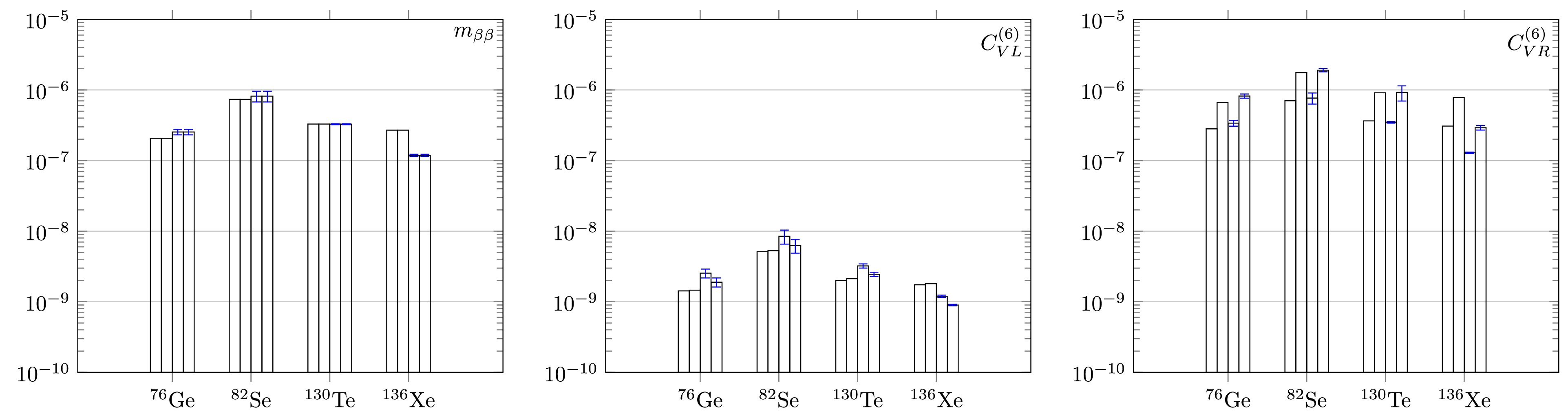
Figure 2. (color online) Experimental constraints on the upper limits of the unknown dimensionless parameters
$ m_{\beta\beta}/m_e $ and$ C's $ . The ordinate in the figure represents the absolute values of various parameters (abscissa), with the red shaded area representing results from QRPA. In addition, for 76Ge and 82Se, the blue filled areas represent results from the jun45 shell model. For 130Te and 136Xe, the blue filled areas represent results from the jj55a shell model. Furthermore, the region filled with lines from the bottom left to the top right indicates the results from Refs. [15, 26], whereas the region filled with lines from the top left to the bottom right indicates our results. In the shell model results, the parameters jj44b and GCN50:82 are introduced as uncertainties.For the case in which the mass mechanism dominates, current experiments set the limit
$ m_{\beta\beta}/m_e $ below$ 10^{-6} $ , which corresponds to$ m_{\beta\beta} $ below 100 meV for 76Ge or 136Xe. These limits are somehow directly related to the calculated NMEs; therefore, they are related to the many-body approaches adopted. For QRPA calculations, the most stringent constraint arises from 76Ge, although the longest half-life limit is obtained from the KamLAND-Zen experiment. The reason has been discussed previously, and once again emphasizes the importance of the determinations of NMEs. Whereas for the LSSM calculation, the constraints of$ m_{\beta\beta} $ generally follow the order of half-life limits, the most stringent one arises from 136Xe owing to a smaller fluctuation in the values of the NMEs for the mass mechanism. Meanwhile, the errors from different Hamiltonians are also illustrated.The suppression of 136Xe from the QRPA calculation mostly arises from a small overlap factor shared by all NMEs. Therefore, the most stringent constraint for the Wilson coefficients
$ C_{VL}^{(6)} $ and$ C_{VR}^{(6} $ also originates from 76Ge for the QRPA calculation, and136Xe for the LSSM calculation. For$ C_{VL}^{(6)} $ , the constraint from the master formula with an IBM calculation [15] yields$ 1.43\times 10^{-9} $ , and we provide a value close to$ 10^{-9} $ for both many-body calculations. Meanwhile, the constraint on$ C_{VR}^{(6)} $ is set to$ 2.81\times 10^{-7} $ , with a vallue between$ 10^{-6}\sim 10^{-7} $ from our calculations.However, as indicated in the above section, the larger deviation in the
$ M_{q} $ term does not cause a significant difference in the determination of the new physics parameters. For the constraint on$ C_{VL}^{(6)} $ , the deviations from the two formalisms are substantially less than those from the two many-body calculations, whereas the opposite holds for$ C_{VR}^{(6)} $ . These results suggest that for the future determination or constraints of new physics parameters, both the realization of the underlying mechanism and nuclear many-body calculations of NMEs are important. -
In this section, we investigate how current experimental data can be used to constrain the parameter space associated with various BSM scenarios contributing to
$ 0\nu\beta\beta $ -decay. Under the assumption that only a single Wilson coefficient dominates the decay process—thus neglecting possible interference between different mechanisms—we utilize the most recent lower bounds on half-lives reported by experiments (see Table 5) to derive constraints on the corresponding new physics parameters. The resulting exclusion limits are illustrated in Fig. 2.Table 5. Current lower limits on the half-lives of
$ 0\nu\beta\beta $ –decay [52].
Figure 2. Experimental constraints on the upper limits of the unknown dimensionless parameters
$ m_{\beta\beta}/m_e $ and$ C's $ . The ordinate in the figure represents the absolute values of various parameters (abscissa), with the red shaded area representing results from QRPA. Additionally, for 76Ge and 82Se, the blue filled areas represent results from the jun45 shell model. For 130Te and 136Xe, the blue filled areas represent results from the jj55a shell model. Furthermore, the region filled with lines from the bottom left to the top right indicates results from Refs. [15, 26], while the region filled with lines from the top left to the bottom right indicates our results. In the shell model results, parameters jj44b and GCN50:82 are introduced as uncertainties.For the case that the mass mechanism dominates, current experiments set the limit
$ m_{\beta\beta}/m_e $ below$ 10^{-6} $ , this corresponds to$ m_{\beta\beta} $ below 100 meV for 76Ge or 136Xe. These limits are somehow directly related to the calculated NMEs, therefore, they are related to the many-body approaches one adopts. For QRPA calculations, the most stringent constraint comes from 76Ge although the longest half-life limit is from KamLAND-Zen experiment. The reason has been discussed above, this once again emphasize the importance of the determinations of NMEs. While for the LSSM calculation, the constraints of$ m_{\beta\beta} $ generally follows the order of half-life limits, the most stringent one comes from 136Xe due to a smaller fluctuation for the values of NMEs for mass mechanism. Meanwhile, the error from different Hamiltonians are also illustrated.Since the suppression of 136Xe from QRPA calculation mostly comes from a small overlap factor which all the NMEs shares. Therefore the most stringent constraints for the Wilson coefficients
$ C_{VL}^{(6)} $ and$ C_{VR}^{(6} $ also comes from 76Ge for the QRPA calculation, while for LSSM calculation 136Xe. For$ C_{VL}^{(6)} $ , the constraints from the master formula with an IBM calculation [15] gives$ 1.43\times 10^{-9} $ , we give a value close to$ 10^{-9} $ for both many-body calculations. For the meantime, a constraints on$ C_{VR}^{(6)} $ was set at$ 2.81\times 10^{-7} $ , and in between$ 10^{-6}\sim 10^{-7} $ from our calculations.On the other hand, as indicated in the above section, the larger deviation in
$ M_{q} $ term doesn't not cause too much difference in the determination of the new physics parameters. For the constraint on$ C_{VL}^{(6)} $ , the deviations from the two formalisms are much less than that from the two many-body calculations. While for$ C_{VR}^{(6)} $ the opposite holds. These suggest that for future determination or constraints of new physics parameters, both the realization of underlying mechanism and the nuclear many-body calculations of NMEs are important. -
In this section, we investigate how current experimental data can be used to constrain the parameter space associated with various BSM scenarios contributing to
$ 0\nu\beta\beta $ -decay. Under the assumption that only a single Wilson coefficient dominates the decay process, and thus, neglecting possible interference between different mechanisms, we utilize the most recent lower bounds on half-lives reported from experiments (see Table 5) to derive constraints on the corresponding new physics parameters. The resulting exclusion limits are illustrated in Fig. 2.Table 5. Current lower limits on the half-lives of
$ 0\nu\beta\beta $ –decay [52].
Figure 2. (color online) Experimental constraints on the upper limits of the unknown dimensionless parameters
$ m_{\beta\beta}/m_e $ and$ C's $ . The ordinate in the figure represents the absolute values of various parameters (abscissa), with the red shaded area representing results from QRPA. In addition, for 76Ge and 82Se, the blue filled areas represent results from the jun45 shell model. For 130Te and 136Xe, the blue filled areas represent results from the jj55a shell model. Furthermore, the region filled with lines from the bottom left to the top right indicates the results from Refs. [15, 26], whereas the region filled with lines from the top left to the bottom right indicates our results. In the shell model results, the parameters jj44b and GCN50:82 are introduced as uncertainties.For the case in which the mass mechanism dominates, current experiments set the limit
$ m_{\beta\beta}/m_e $ below$ 10^{-6} $ , which corresponds to$ m_{\beta\beta} $ below 100 meV for 76Ge or 136Xe. These limits are somehow directly related to the calculated NMEs; therefore, they are related to the many-body approaches adopted. For QRPA calculations, the most stringent constraint arises from 76Ge, although the longest half-life limit is obtained from the KamLAND-Zen experiment. The reason has been discussed previously, and once again emphasizes the importance of the determinations of NMEs. Whereas for the LSSM calculation, the constraints of$ m_{\beta\beta} $ generally follow the order of half-life limits, the most stringent one arises from 136Xe owing to a smaller fluctuation in the values of the NMEs for the mass mechanism. Meanwhile, the errors from different Hamiltonians are also illustrated.The suppression of 136Xe from the QRPA calculation mostly arises from a small overlap factor shared by all NMEs. Therefore, the most stringent constraint for the Wilson coefficients
$ C_{VL}^{(6)} $ and$ C_{VR}^{(6} $ also originates from 76Ge for the QRPA calculation, and136Xe for the LSSM calculation. For$ C_{VL}^{(6)} $ , the constraint from the master formula with an IBM calculation [15] yields$ 1.43\times 10^{-9} $ , and we provide a value close to$ 10^{-9} $ for both many-body calculations. Meanwhile, the constraint on$ C_{VR}^{(6)} $ is set to$ 2.81\times 10^{-7} $ , with a vallue between$ 10^{-6}\sim 10^{-7} $ from our calculations.However, as indicated in the above section, the larger deviation in the
$ M_{q} $ term does not cause a significant difference in the determination of the new physics parameters. For the constraint on$ C_{VL}^{(6)} $ , the deviations from the two formalisms are substantially less than those from the two many-body calculations, whereas the opposite holds for$ C_{VR}^{(6)} $ . These results suggest that for the future determination or constraints of new physics parameters, both the realization of the underlying mechanism and nuclear many-body calculations of NMEs are important. -
In the framework of χEFT, we simulated the contribution of dim-6 operators in LEFT originating from SMEFT dim-7 operators relevant to the LRSM for the
$ 0\nu\beta\beta $ –decay half-life based on the S-matrix theory, obtaining results consistent with previous new physics model calculations [19]. We compared our results with the so-called master formula in Ref. [26]. We observed decent agreement between these two frameworks. Furthermore, we found that the counterpart of the q term NMEs in Ref. [26] was smaller than our results, emphasizing the effects of distortion of electron wave functions from nuclear electrical static potential. We further provided constraints on the Wilson coefficients of relevant LEFT operators by utilizing current experimental limits. -
In the framework of χEFT, we simulate the contribution of Dim-6 operators in LEFT originating from SMEFT Dim-7 operators relevant to the LRSM to the
$ 0\nu\beta\beta $ –decay half-life based on the S-matrix theory, obtaining results consistent with previous new physics model calculations [19]. We compare our results with the so-called master formula in Ref. [26]. We find decent agreement between these two frameworks. Furthermore, we observe that counterpart of the q-term NMEs in Ref. [26] is smaller than our results, emphasizing the effects of distortion of electron wave functions from nuclear electrical static potential. We further give constraints on the constraints of the Wilson coefficients of relevant LEFT operators by utilizing current experimental limits. -
In the framework of χEFT, we simulated the contribution of dim-6 operators in LEFT originating from SMEFT dim-7 operators relevant to the LRSM for the
$ 0\nu\beta\beta $ –decay half-life based on the S-matrix theory, obtaining results consistent with previous new physics model calculations [19]. We compared our results with the so-called master formula in Ref. [26]. We observed decent agreement between these two frameworks. Furthermore, we found that the counterpart of the q term NMEs in Ref. [26] was smaller than our results, emphasizing the effects of distortion of electron wave functions from nuclear electrical static potential. We further provided constraints on the Wilson coefficients of relevant LEFT operators by utilizing current experimental limits. -
The electron wave function
$ \psi(\epsilon,{\boldsymbol{r}}) $ is described as a combination of spherical waves distorted by Coulomb forces and the wave functions for specific partial waves can be solved numerically by subroutines Radial [65].In general, these electron wave functions can be decomposed into different partial waves as:
$ \begin{aligned} \psi(\epsilon,{\boldsymbol{r}})=\psi^{(S)}(\epsilon,{\boldsymbol{r}})+\psi^{(P)}(\epsilon,{\boldsymbol{r}})+\psi^{(D)}(\epsilon,{\boldsymbol{r}})+\cdots. \end{aligned} $

(A1) Here S, P and D respectively represent the S(l=0)-, P(l=1)- and D(l=2)-waves etc.
In current work, higher partial waves except P-wave are neglected in the calculations. The S-wave and P-wave forms can be expressed respectively as [19]:
$ \begin{aligned}[b]& \psi^{(S)}(\epsilon,{\boldsymbol{r}}) =\begin{pmatrix} g_{-1}\chi_s\\ \left({\boldsymbol{\sigma}}\cdot\hat{{\boldsymbol{p}}}\right)f_1\chi_s \end{pmatrix},\\&\psi^{(P)}(\epsilon,{\boldsymbol{r}})=\\&i \begin{pmatrix} \left(g_1\left({\boldsymbol{\sigma}}\cdot\hat{{\boldsymbol{r}}}\right)\left({\boldsymbol{\sigma}}\cdot\hat{{\boldsymbol{p}}}\right)+g_{-2}\left[3\left(\hat{{\boldsymbol{r}}}\cdot\hat{{\boldsymbol{p}}}\right)-\left({\boldsymbol{\sigma}}\cdot\hat{{\boldsymbol{r}}}\right)\left({\boldsymbol{\sigma}}\cdot\hat{{\boldsymbol{p}}}\right)\right]\right)\chi_s\\ \left(-f_{-1}\left({\boldsymbol{\sigma}}\cdot\hat{{\boldsymbol{r}}}\right)+f_2\left[3\left({\boldsymbol{\sigma}}\cdot\hat{{\boldsymbol{r}}}\right)\left({\boldsymbol{\sigma}}\cdot\hat{{\boldsymbol{p}}}\right)-\left({\boldsymbol{\sigma}}\cdot\hat{{\boldsymbol{r}}}\right)\right]\right)\chi_s \end{pmatrix}. \end{aligned} $

(A2) To facilitate the calculation of the
$ 0\nu\beta\beta $ –decay scattering amplitudes in Appendix C, we define following functionals of electron wave functions [19]:$ \begin{aligned}[b] t^L_{\mu\nu}\left(\epsilon_1{\boldsymbol{x}},\epsilon_2{\boldsymbol{y}}\right)&=\bar{\psi}\left(\epsilon_1,{\boldsymbol{x}}\right)\gamma_\mu\left(1-\gamma_5\right)\gamma_\nu\psi^C\left(\epsilon_2,{\boldsymbol{y}}\right),\\ u^{L(R)}_{\mu\nu}\left(\epsilon_1{\boldsymbol{x}},\epsilon_2{\boldsymbol{y}}\right)&=q^\rho\bar{\psi}\left(\epsilon_1,{\boldsymbol{x}}\right)\gamma_\mu\left(1\mp\gamma_5\right)\gamma_\rho\gamma_\nu\psi^C\left(\epsilon_2,{\boldsymbol{y}}\right),\\ t^{L(R)}\left(\epsilon_1{\boldsymbol{x}},\epsilon_2{\boldsymbol{y}}\right)&=\bar{\psi}\left(\epsilon_1,{\boldsymbol{x}}\right)\left(1\pm\gamma_5\right)\psi^C\left(\epsilon_2,{\boldsymbol{y}}\right),\\ u^{L(R)}_{\mu}\left(\epsilon_1{\boldsymbol{x}},\epsilon_2{\boldsymbol{y}}\right)&=\bar{\psi}\left(\epsilon_1,{\boldsymbol{x}}\right)\gamma_\mu\left(1\mp\gamma_5\right)\psi^C\left(\epsilon_2,{\boldsymbol{y}}\right). \end{aligned} $

(A3) As well as
$ \begin{aligned}[b] u_{\mu}(\epsilon_1 {\boldsymbol{x}},\epsilon_2 {\boldsymbol{y}})&= \bar{\psi}(\epsilon_1,{\boldsymbol{x}})\gamma_\mu\psi^C(\epsilon_2,{\boldsymbol{y}}),\\ u^{(5)}_{\mu}(\epsilon_1 {\boldsymbol{x}},\epsilon_2 {\boldsymbol{y}})&=\bar{\psi}(\epsilon_1,{\boldsymbol{x}}) \gamma_\mu\gamma_5\psi^C(\epsilon_2,{\boldsymbol{y}}). \end{aligned} $

(A4) More functionals are defined following [19]:
$ \begin{aligned} F_{\mu\pm}(\epsilon_1{\boldsymbol{x}},\epsilon_2{\boldsymbol{y}})&=\frac{u_\mu(\epsilon_1{\boldsymbol{x}},\epsilon_2 {\boldsymbol{y}})\pm u_\mu(\epsilon_1{\boldsymbol{y}},\epsilon_2{\boldsymbol{y}})}{2}, \\ F_{\mu\pm}^{(5)}(\epsilon_1{\boldsymbol{x}},\epsilon_2{\boldsymbol{y}})&=\frac{u^{(5)}_\mu(\epsilon_1{\boldsymbol{x}},\epsilon_2 {\boldsymbol{y}})\pm u^{(5)}_\mu(\epsilon_1{\boldsymbol{y}},\epsilon_2{\boldsymbol{y}})}{2}. \end{aligned} $

(A5) Where for the time component, the dominant contribution are for both electrons with s partial-wave, while for the spatial component, at least one electron should be with p partial wave. For the latter case, one can extract out a factor
$ {\boldsymbol{r}}/2 $ and$ {\boldsymbol{r}}_+ $ and redefine the F functionals:$ \begin{aligned}[b] F_{i-}(\epsilon_1 {\boldsymbol{x}},\epsilon_2 {\boldsymbol{y}})&= \frac{r_i}{2} {\cal{F}}_-(\epsilon_1 {\boldsymbol{x}},\epsilon_2 {\boldsymbol{y}}), \\ F_{i+}(\epsilon_1 {\boldsymbol{x}},\epsilon_2 {\boldsymbol{y}})&= r_{+i} {\cal{F}}_+(\epsilon_1 {\boldsymbol{x}},\epsilon_2 {\boldsymbol{y}}), \\ F^{(5)}_{i-}(\epsilon_1 {\boldsymbol{x}},\epsilon_2 {\boldsymbol{y}})&= r_{+i} {\cal{F}}_-^{(5)}(\epsilon_1 {\boldsymbol{x}},\epsilon_2 {\boldsymbol{y}}), \\ F^{(5)}_{i+}(\epsilon_1 {\boldsymbol{x}},\epsilon_2 {\boldsymbol{y}})&= \frac{r_i}{2}{\cal{F}}_+^{(5)}(\epsilon_1 {\boldsymbol{x}},\epsilon_2 {\boldsymbol{y}}). \end{aligned} $

(A6) Here,
$ {\boldsymbol{r}}_+=({\boldsymbol{r}}_1+{\boldsymbol{r}}_2)/2 $ , and$ {\boldsymbol{r}}={\boldsymbol{r}}_1-{\boldsymbol{r}}_2 $ . -
The electron wave function
$ \psi(\epsilon,{\boldsymbol{r}}) $ is described as a combination of spherical waves distorted by Coulomb forces, and the wave functions for specific partial waves can be solved numerically using the subroutines Radial [64].In general, these electron wave functions can be decomposed into different partial waves as follows:
$ \begin{aligned} \psi(\epsilon,{\boldsymbol{r}})=\psi^{(S)}(\epsilon,{\boldsymbol{r}})+\psi^{(P)}(\epsilon,{\boldsymbol{r}})+\psi^{(D)}(\epsilon,{\boldsymbol{r}})+\cdots. \end{aligned} $
(A1) Here, S, P, and I respectively represent the S(l=0)-, P(l=1)-, and D(l=2)-waves.
In the current work, higher partial waves except for the P-wave are neglected in the calculations. The S-wave and P-wave forms can be expressed respectively as [19]
$ \begin{aligned}[b]& \psi^{(S)}(\epsilon,{\boldsymbol{r}}) =\begin{pmatrix} g_{-1}\chi_s\\ \left({\boldsymbol{\sigma}}\cdot\hat{{\boldsymbol{p}}}\right)f_1\chi_s \end{pmatrix},\\&\psi^{(P)}(\epsilon,{\boldsymbol{r}})=\\&i \begin{pmatrix} \left(g_1\left({\boldsymbol{\sigma}}\cdot\hat{{\boldsymbol{r}}}\right)\left({\boldsymbol{\sigma}}\cdot\hat{{\boldsymbol{p}}}\right)+g_{-2}\left[3\left(\hat{{\boldsymbol{r}}}\cdot\hat{{\boldsymbol{p}}}\right)-\left({\boldsymbol{\sigma}}\cdot\hat{{\boldsymbol{r}}}\right)\left({\boldsymbol{\sigma}}\cdot\hat{{\boldsymbol{p}}}\right)\right]\right)\chi_s\\ \left(-f_{-1}\left({\boldsymbol{\sigma}}\cdot\hat{{\boldsymbol{r}}}\right)+f_2\left[3\left({\boldsymbol{\sigma}}\cdot\hat{{\boldsymbol{r}}}\right)\left({\boldsymbol{\sigma}}\cdot\hat{{\boldsymbol{p}}}\right)-\left({\boldsymbol{\sigma}}\cdot\hat{{\boldsymbol{r}}}\right)\right]\right)\chi_s \end{pmatrix}. \end{aligned} $
(A2) To facilitate the calculation of the
$ 0\nu\beta\beta $ –decay scattering amplitudes in Appendix C, we define the following functionals of the electron wave functions [19]:$ \begin{aligned}[b] t^L_{\mu\nu}\left(\epsilon_1{\boldsymbol{x}},\epsilon_2{\boldsymbol{y}}\right)&=\bar{\psi}\left(\epsilon_1,{\boldsymbol{x}}\right)\gamma_\mu\left(1-\gamma_5\right)\gamma_\nu\psi^C\left(\epsilon_2,{\boldsymbol{y}}\right),\\ u^{L(R)}_{\mu\nu}\left(\epsilon_1{\boldsymbol{x}},\epsilon_2{\boldsymbol{y}}\right)&=q^\rho\bar{\psi}\left(\epsilon_1,{\boldsymbol{x}}\right)\gamma_\mu\left(1\mp\gamma_5\right)\gamma_\rho\gamma_\nu\psi^C\left(\epsilon_2,{\boldsymbol{y}}\right),\\ t^{L(R)}\left(\epsilon_1{\boldsymbol{x}},\epsilon_2{\boldsymbol{y}}\right)&=\bar{\psi}\left(\epsilon_1,{\boldsymbol{x}}\right)\left(1\pm\gamma_5\right)\psi^C\left(\epsilon_2,{\boldsymbol{y}}\right),\\ u^{L(R)}_{\mu}\left(\epsilon_1{\boldsymbol{x}},\epsilon_2{\boldsymbol{y}}\right)&=\bar{\psi}\left(\epsilon_1,{\boldsymbol{x}}\right)\gamma_\mu\left(1\mp\gamma_5\right)\psi^C\left(\epsilon_2,{\boldsymbol{y}}\right). \end{aligned} $
(A3) In addition,
$ \begin{aligned}[b] u_{\mu}(\epsilon_1 {\boldsymbol{x}},\epsilon_2 {\boldsymbol{y}})&= \bar{\psi}(\epsilon_1,{\boldsymbol{x}})\gamma_\mu\psi^C(\epsilon_2,{\boldsymbol{y}}),\\ u^{(5)}_{\mu}(\epsilon_1 {\boldsymbol{x}},\epsilon_2 {\boldsymbol{y}})&=\bar{\psi}(\epsilon_1,{\boldsymbol{x}}) \gamma_\mu\gamma_5\psi^C(\epsilon_2,{\boldsymbol{y}}). \end{aligned} $
(A4) Further functionals are defined following [19]:
$ \begin{aligned} F_{\mu\pm}(\epsilon_1{\boldsymbol{x}},\epsilon_2{\boldsymbol{y}})&=\frac{u_\mu(\epsilon_1{\boldsymbol{x}},\epsilon_2 {\boldsymbol{y}})\pm u_\mu(\epsilon_1{\boldsymbol{y}},\epsilon_2{\boldsymbol{x}})}{2}, \\ F_{\mu\pm}^{(5)}(\epsilon_1{\boldsymbol{x}},\epsilon_2{\boldsymbol{y}})&=\frac{u^{(5)}_\mu(\epsilon_1{\boldsymbol{x}},\epsilon_2 {\boldsymbol{y}})\pm u^{(5)}_\mu(\epsilon_1{\boldsymbol{y}},\epsilon_2{\boldsymbol{x}})}{2}. \end{aligned} $
(A5) For the time component, the dominant contributions are for both electrons with s partial-waves, while for the spatial component, at least one electron should have a p partial wave. For the latter case, one can extract out the factor
$ {\boldsymbol{r}}/2 $ and$ {\boldsymbol{r}}_+ $ and redefine the F functionals:$ \begin{aligned}[b] F_{i-}(\epsilon_1 {\boldsymbol{x}},\epsilon_2 {\boldsymbol{y}})&= \frac{r_i}{2} {\cal{F}}_-(\epsilon_1 {\boldsymbol{x}},\epsilon_2 {\boldsymbol{y}}), \\ F_{i+}(\epsilon_1 {\boldsymbol{x}},\epsilon_2 {\boldsymbol{y}})&= r_{+i} {\cal{F}}_+(\epsilon_1 {\boldsymbol{x}},\epsilon_2 {\boldsymbol{y}}), \\ F^{(5)}_{i-}(\epsilon_1 {\boldsymbol{x}},\epsilon_2 {\boldsymbol{y}})&= r_{+i} {\cal{F}}_-^{(5)}(\epsilon_1 {\boldsymbol{x}},\epsilon_2 {\boldsymbol{y}}), \\ F^{(5)}_{i+}(\epsilon_1 {\boldsymbol{x}},\epsilon_2 {\boldsymbol{y}})&= \frac{r_i}{2}{\cal{F}}_+^{(5)}(\epsilon_1 {\boldsymbol{x}},\epsilon_2 {\boldsymbol{y}}). \end{aligned} $
(A6) Here,
$ {\boldsymbol{r}}_+=({\boldsymbol{r}}_1+{\boldsymbol{r}}_2)/2 $ and$ {\boldsymbol{r}}={\boldsymbol{r}}_1-{\boldsymbol{r}}_2 $ . -
In this section, we provide detailed definitions of the nuclear matrix elements and neutrino potentials. The contributions from the neutrino mass term, as well as from qL, qR,
$ \omega L $ , and$ \omega R $ , can be written in a unified form as the sum of three components [19]:$ \begin{aligned} M_i=M_{iF}+M_{iGT}+M_{iT}. \end{aligned} $
(B1) In addition, the GT and tensor parts are composed of different components:
$ \begin{aligned} M_{iGT}&=M_{iGT}^{AA}+M_{iGT}^{AP}+M_{iGT}^{PP}+M_{iGT}^{MM},\\ M_{iT}&=M_{iT}^{AA}+M_{iT}^{AP}+M_{iT}^{PP}+M_{iT}^{MM}. \end{aligned} $
(B2) It is worth noting that, within the defined nuclear matrix elements, the tensor contribution from the AA current arises solely in the q-type terms and does not appear in the matrix elements corresponding to the mass mechanism or ω-type terms. Based on these definitions, the following relations hold among the nuclear matrix elements:
$ \begin{aligned}[b]& M_{\nu F}=-M_F, \quad M_{qLF}=-M_{qF}, \quad M_{\omega LF}=M_{\omega F}, \\& M_{qRF}=M_{qF},\quad M_{\omega RF}=-M_{\omega F}, \quad M^{ij}_{\nu GT}=M^{ij}_{GT}, \\& M^{ij}_{\nu T}=M^{ij}_T, \quad M^{ij}_{qLGT}=M^{ij}_{qGT},\quad M^{ij}_{qLT}=M^{ij}_{qT}, \\& M^{ij}_{\omega LGT}=M^{ij}_{\omega GT}, \quad M^{ij}_{\omega LT}=M^{ij}_{\omega T}, \quad M^{ij}_{qRGT}=M^{ij}_{qGT},\\& M^{ij}_{qRT}=M^{ij}_{qT}, \quad M^{ij}_{\omega RGT}=M^{ij}_{\omega GT}, \quad M^{ij}_{\omega RT}=M^{ij}_{qT}. \end{aligned} $
(B3) Special attention should be paid to the following exceptions, which apply specifically to the MM components:
$ \begin{aligned}[b] M_{\nu T}^{MM}&=0\neq M_T^{MM}, \quad M_{qRGT}^{MM}= -M_{qGT}^{MM},\quad M_{qRT}^{MM} = -M_{qT}^{MM},\\ M_{\omega RGT}^{MM} &= -M_{\omega GT}^{MM}, \quad M_{\omega RT}^{MM} = -M_{\omega T}^{MM}. \end{aligned} $
(B4) In contrast, the expression for the R-term is relatively simple:
$ \begin{aligned} M_R&=M_{RGT}+M_{RT}. \end{aligned}$
(B5) The P-term, denoted by
$ M_P $ , consists of a single component, the structure of which is presented below.More generally, all of the above nuclear matrix elements can be expressed in the following unified form:
$ \begin{aligned} M^{ij}_{KI}&=\sum_{n,m}\left\langle N_f\right| h_{K I}^{i j}\left(r_{n m}, r_{n m}^+\right) \tau_n^+ \tau_m^+ {\cal{O}}_I\left|N_i\right\rangle, \end{aligned} $
(B6) with the radial
$ h_{I}^{ij}(r_{nm},r^+_{nm}) $ (neutrino potential) and angular$ {\cal{O}}_I $ parts. Here, K refers to different mechanisms.The angular operator
$ {\cal{O}}_I $ 's have the form [19, 28]$ \begin{aligned}[b]& {\cal{O}}_{F}=1, \quad {\cal{O}}_{GT}= {\boldsymbol{\sigma}}_{n}\cdot {\boldsymbol{\sigma}}_{m},\\& {\cal{O}}_{T}=3{\boldsymbol{\sigma}}_{n}\cdot\hat{{\boldsymbol{r}}}_{nm} {\boldsymbol{\sigma}}_{m}\cdot\hat{{\boldsymbol{r}}}_{nm}- {\boldsymbol{\sigma}}_{n}\cdot {\boldsymbol{\sigma}}_{m}, \\& {\cal{O}}_{P}=i\left({\boldsymbol{\sigma}}_{n}-{\boldsymbol{\sigma}}_{m}\right)\cdot\left(\hat{{\boldsymbol{r}}}_{nm}\times\hat{{\boldsymbol{r}}}_{+nm}\right), \end{aligned} $
(B7) where
$ {\boldsymbol{r}}_{nm} = {\boldsymbol{r}}_n - {\boldsymbol{r}}_m $ represents the relative position between the mth nucleon and nth nucleon, while$ {\boldsymbol{r}}^+_{nm} = ({\boldsymbol{r}}_n + {\boldsymbol{r}}_m)/2 $ denotes the center of mass coordinates between them, with$ \hat{{\boldsymbol{r}}}_{nm} $ representing a unit vector in the direction of$ {\boldsymbol{r}}_{nm} $ and similarly$ \hat{{\boldsymbol{r}}}^+_{nm} $ .The neutrino potential can generally be expressed as
$ \begin{aligned} h^{ij}_I(r,r_+)=\frac{2R}{\pi}\int_0^\infty f^{ij}_I(q,r,r_+)\frac{q{\rm d}q}{q+E_a-\left(E_i+E_f\right)/2}, \end{aligned} $
(B8) except for the ω terms, for which the form of the neutrino potential changes to
$ \begin{aligned} h^{ij}_I(r,r_+)=\frac{2R}{\pi}\int_0^\infty f^{ij}_I(q,r,r_+)\frac{q^2{\rm d}q}{\left(q+E_a-\left(E_i+E_f\right)/2\right)^2}. \end{aligned} $
(B9) Here, R represents the nuclear radius, which is introduced to make the neutrino potential dimensionless overall.
$ E_a $ denotes the energy of the intermediate state in the nucleus, while$ E_i $ and$ E_j $ represent the energies of the parent and daughter nuclei, respectively. In the QRPA calculations, the intermediate states are explicitly included and$ E_a $ is obtained from the QRPA solutions [52]. In the LSSM calculation, the closure approximation is adopted, and an average closure energy of 7 MeV is used [51].The detailed expressions for each component are as follows:
1) mass term or ω term
$ \begin{aligned}[b]& f_{F}=g^2_V(q^2)j_0\left(qr\right), \quad f^{AA}_{T,GT}=g^2_A(q^2)j_{2,0}\left(qr\right), \\& f^{AP}_{GT}={g_A(q^2)g_P(q^2)}\frac{q^2}{3m_N}j_0\left(qr\right),\quad f^{PP}_{GT}={g^2_P(q^2)}\frac{q^4}{12m^2_N}j_0\left(qr\right),\\& f^{MM}_{GT}={g^2_M(q^2)}\frac{q^2}{6m^2_N}j_0\left(qr\right),\\& f^{AP}_{T}=-g_A(q^2)g_P(q^2)\frac{q^2}{3m_N}j_2\left(qr\right),\\& f^{PP}_{T}=-g^2_P(q^2)\frac{q^4}{12m^2_N}j_2\left(qr\right), \\& f^{MM}_{T}=g^2_M(q^2)\frac{q^2}{12m^2_N}j_2\left(qr\right). \end{aligned} $
(B10) 2) q term
$ \begin{aligned}[b]& f_{qF}=g^2_V(q^2)j_1(qr)qr,\quad f^{AA}_{qGT}=g^2_A(q^2)\frac{1}{3}j_1(qr)qr, \\& f^{AP}_{qGT}=-g_A(q^2)g_P(q^2)\frac{q^2}{3m_N}j_1(qr)qr,\\& f^{PP}_{qGT}=-g^2_P(q^2)\frac{q^4}{12m^2_N}j_1(qr)qr, \\& f^{MM}_{qGT}=g^2_M(q^2)\frac{q^2}{6m^2_N}j_1(qr)qr, \quad f^{AA}_{qT}=-g^2_A(q^2)\frac{2}{3}j_1(qr)qr,\\& f^{AP}_{qT}=-g_A(q^2)g_P(q^2)\frac{q^2}{3m_N}j_1(qr)qr, \\& f^{PP}_{qT}=-g^2_P(q^2)\frac{q^4}{20m^2_N}\left(\frac{2}{3}j_1(qr)-j_3(qr)\right)qr,\\& f^{MM}_{qT}=-g^2_M(q^2)\frac{q^2}{20m^2_N}\left(\frac{2}{3}j_1(qr)-j_3(qr)\right)qr. \end{aligned} $
(B11) 3) R term
$ \begin{aligned}[b] &f_{RGT}=-g_A(q^2)g_M(q^2)\frac{R}{3m_N}j_0(qr)q^2, \\& f_{RT}=-g_A(q^2)g_M(q^2)\frac{R}{6m_N}j_2(qr)q^2. \end{aligned} $
(B12) 4) P term
$ \begin{aligned} f_P=g_V(q^2)g_A(q^2)j_1(qr)qr_+. \end{aligned} $
(B13) Here,
$ j_0 $ ,$ j_1 $ ,$ j_2 $ , and$ j_3 $ are spherical Bessel functions of the specific ranks.$ f_{T}^{AA} $ does not appear in our calculation but is part of the master formula in Ref. [15]. In addition, compared with the expressions in Refs. [19, 28, 51], we absorb the factor 1/3 into the definition of the NMEs to obtain a compact expression for q terms.We also compare our results with those from the so-called master formula, which consist of components from the mass term in Eq. (B10). We define the NMEs out of the amplitudes in Ref. [15] by extracting the corresponding Wilson coefficients:
$ \begin{aligned}[b] M_{E,L}=\;&\frac{1}{3}\left(M_F+\frac{1}{3}\left(2M_{GT}^{AA}+M_{T}^{AA}\right)\right), \\ M_{E,R}=\;&\frac{1}{3}\left(M_F-\frac{1}{3}\left(2M_{GT}^{AA}+M_T^{AA}\right)\right), \\ M_{m_e,L}=\;&-\frac{1}{6}\Bigg(M_F-\frac{1}{3}\left(M_{GT}^{AA}-4M_T^{AA}\right)\\&-3\left(M^{AP}_{GT}+M_{GT}^{PP}+M_T^{AP}+M_{T}^{PP}\right)\Bigg), \\ M_{m_e,R}=\;&-\frac{1}{6}\Bigg(M_F+\frac{1}{3}\left(M_{GT}^{AA}-4M_T^{AA}\right) \end{aligned} $
$ \begin{aligned}[b]&+3\left(M^{AP}_{GT}+M_{GT}^{PP}+M_T^{AP}+M_{T}^{PP}\right)\Bigg), \\ M_M=&-2\frac{g_A}{g_M}(M_{GT}^{MM}+M_T^{MM}). \end{aligned} $
(B14) Here, both
$ M_{m_e,L} $ and$ M_{m_e,R} $ contain contributions from the q- and ω-dependent terms. To facilitate the classification and comparison of these contributions, we reorganize the expressions in terms of the q, ω, and R structures, yielding a more compact representation:$ \begin{aligned}[b] M'_{\omega L}&=4\left(M_{E,L}+M_{m_e,L}/2\right), \quad M'_{\omega R}=-4\left(M_{E,R}+M_{m_e,R}/2\right),\\ M'_{q L}&=6M_{m_e,L}, \quad M'_{q R}=-6M_{m_e,R}, \quad M'_{R}=-m_NRM_M.\end{aligned} $
(B15) The purpose of this decomposition is to express the results in a form consistent with Eq. (19), thereby allowing for a direct identification of the matrix elements defined in Eq. (20). This representation facilitates a systematic comparison of the contributions from each term, as shown in Table 4.
-
In this section, we provide detailed definitions of the nuclear matrix elements and neutrino potentials. The contributions from the neutrino mass term, as well as from qL, qR,
$ \omega L $ , and$ \omega R $ , can be written in a unified form as the sum of three components [19]:$ \begin{aligned} M_i=M_{iF}+M_{iGT}+M_{iT}. \end{aligned} $

(B1) And the GT and Tensor parts are composed of different components:
$ \begin{aligned} M_{iGT}&=M_{iGT}^{AA}+M_{iGT}^{AP}+M_{iGT}^{PP}+M_{iGT}^{MM},\\ M_{iT}&=M_{iT}^{AA}+M_{iT}^{AP}+M_{iT}^{PP}+M_{iT}^{MM}. \end{aligned} $

(B2) It is worth noting that, within the defined nuclear matrix elements, the tensor contribution from the AA current arises solely in the q-type terms and does not appear in the matrix elements corresponding to the mass mechanism or ω-type terms. Based on these definitions, the following relations hold among the nuclear matrix elements:
$ \begin{aligned}[b]& M_{\nu F}=-M_F, \quad M_{qLF}=-M_{qF}, \quad M_{\omega LF}=M_{\omega F}, \\& M_{qRF}=M_{qF},\quad M_{\omega RF}=-M_{\omega F}, \quad M^{ij}_{\nu GT}=M^{ij}_{GT}, \\& M^{ij}_{\nu T}=M^{ij}_T, \quad M^{ij}_{qLGT}=M^{ij}_{qGT},\quad M^{ij}_{qLT}=M^{ij}_{qT}, \\& M^{ij}_{\omega LGT}=M^{ij}_{\omega GT}, \quad M^{ij}_{\omega LT}=M^{ij}_{\omega T}, \quad M^{ij}_{qRGT}=M^{ij}_{qGT},\\& M^{ij}_{qRT}=M^{ij}_{qT}, \quad M^{ij}_{\omega RGT}=M^{ij}_{\omega GT}, \quad M^{ij}_{\omega RT}=M^{ij}_{qT}. \end{aligned} $

(B3) Special attention should be paid to the following exceptions, which apply specifically to the MM components:
$ \begin{aligned}[b] M_{\nu T}^{MM}&=0\neq M_T^{MM}, \quad M_{qRGT}^{MM}= -M_{qGT}^{MM},\quad M_{qRT}^{MM} = -M_{qT}^{MM},\\ M_{\omega RGT}^{MM} &= -M_{\omega GT}^{MM}, \quad M_{\omega RT}^{MM} = -M_{\omega T}^{MM}. \end{aligned} $

(B4) While the expression for the R-term are relatively simple:
$ \begin{aligned} M_R&=M_{RGT}+M_{RT}. \end{aligned}$

(B5) The P-term, denoted by
$ M_P $ , consists of a single component, whose structure will be presented below.More generally, all of the above nuclear matrix elements can be expressed in the following unified form:
$ \begin{aligned} M^{ij}_{KI}&=\sum_{n,m}\left\langle N_f\right| h_{K I}^{i j}\left(r_{n m}, r_{n m}^+\right) \tau_n^+ \tau_m^+ {\cal{O}}_I\left|N_i\right\rangle, \end{aligned} $

(B6) with the radial
$ h_{I}^{ij}(r_{nm},r^+_{nm}) $ (neutrino potential) and angular$ {\cal{O}}_I $ parts. Here K refers to different mechanisms.The angular operator
$ {\cal{O}}_I $ 's have the form [19, 28]:$ \begin{aligned}[b]& {\cal{O}}_{F}=1, \quad {\cal{O}}_{GT}= {\boldsymbol{\sigma}}_{n}\cdot {\boldsymbol{\sigma}}_{m},\\& {\cal{O}}_{T}=3{\boldsymbol{\sigma}}_{n}\cdot\hat{{\boldsymbol{r}}}_{nm} {\boldsymbol{\sigma}}_{m}\cdot\hat{{\boldsymbol{r}}}_{nm}- {\boldsymbol{\sigma}}_{n}\cdot {\boldsymbol{\sigma}}_{m}, \\& {\cal{O}}_{P}=i\left({\boldsymbol{\sigma}}_{n}-{\boldsymbol{\sigma}}_{m}\right)\cdot\left(\hat{{\boldsymbol{r}}}_{nm}\times\hat{{\boldsymbol{r}}}_{+nm}\right), \end{aligned} $

(B7) where
$ {\boldsymbol{r}}_{nm} = {\boldsymbol{r}}_n - {\boldsymbol{r}}_m $ represents the relative position between the mth nucleon and the nth nucleon, while$ {\boldsymbol{r}}^+_{nm} = ({\boldsymbol{r}}_n + {\boldsymbol{r}}_m)/2 $ is the center of mass coordinates between them, with$ \hat{{\boldsymbol{r}}}_{nm} $ representing a unit vector in the direction of$ {\boldsymbol{r}}_{nm} $ and similarly$ \hat{{\boldsymbol{r}}}^+_{nm} $ .The neutrino potential can be generally expressed as
$ \begin{aligned} h^{ij}_I(r,r_+)=\frac{2R}{\pi}\int_0^\infty f^{ij}_I(q,r,r_+)\frac{qdq}{q+E_a-\left(E_i+E_f\right)/2}. \end{aligned} $

(B8) Except for ω terms, for which the form of the neutrino potential changes to
$ \begin{aligned} h^{ij}_I(r,r_+)=\frac{2R}{\pi}\int_0^\infty f^{ij}_I(q,r,r_+)\frac{q^2dq}{\left(q+E_a-\left(E_i+E_f\right)/2\right)^2}. \end{aligned} $

(B9) Here, R represents the nuclear radius, introduced to make the neutrino potential dimensionless overall.
$ E_a $ denotes the energy of the intermediate state in the nucleus, while$ E_i $ and$ E_j $ represent the energies of the parent and daughter nuclei, respectively. In the QRPA calculations, the intermediate states are explicitly included,$ E_a $ is obtained from the QRPA solutions [53]. While in LSSM calculation, the closure approximation is adopted, and an average closure energy of 7 MeV is used [52].The detailed expressions for each component is given as:
1) mass term or ω term
$ \begin{aligned}[b]& f_{F}=g^2_V(q^2)j_0\left(qr\right), \quad f^{AA}_{T,GT}=g^2_A(q^2)j_0\left(qr\right), \\& f^{AP}_{GT}={g_A(q^2)g_P(q^2)}\frac{q^2}{3m_N}j_0\left(qr\right),\quad f^{PP}_{GT}={g^2_P(q^2)}\frac{q^4}{12m^2_N}j_0\left(qr\right),\\& f^{MM}_{GT}={g^2_M(q^2)}\frac{q^2}{6m^2_N}j_0\left(qr\right),\\& f^{AP}_{T}=-g_A(q^2)g_P(q^2)\frac{q^2}{3m_N}j_2\left(qr\right),\\& f^{PP}_{T}=-g^2_P(q^2)\frac{q^4}{12m^2_N}j_2\left(qr\right), \\& f^{MM}_{T}=g^2_M(q^2)\frac{q^2}{12m^2_N}j_2\left(qr\right). \end{aligned} $

(B10) 2) q term
$ \begin{aligned}[b]& f_{qF}=g^2_V(q^2)j_1(qr)qr,\quad f^{AA}_{qGT}=g^2_A(q^2)\frac{1}{3}j_1(qr)qr, \\& f^{AP}_{qGT}=-g_A(q^2)g_P(q^2)\frac{q^2}{3m_N}j_1(qr)qr,\\& f^{PP}_{qGT}=-g^2_P(q^2)\frac{q^4}{12m^2_N}j_1(qr)qr, \\& f^{MM}_{qGT}=g^2_M(q^2)\frac{q^2}{6m^2_N}j_1(qr)qr, \quad f^{AA}_{qT}=-g^2_A(q^2)\frac{2}{3}j_1(qr)qr,\\& f^{AP}_{qT}=-g_A(q^2)g_P(q^2)\frac{q^2}{3m_N}j_1(qr)qr, \\& f^{PP}_{qT}=-g^2_P(q^2)\frac{q^4}{20m^2_N}\left(\frac{2}{3}j_1(qr)-j_3(qr)\right)qr,\\& f^{MM}_{qT}=-g^2_M(q^2)\frac{q^2}{20m^2_N}\left(\frac{2}{3}j_1(qr)-j_3(qr)\right)qr. \end{aligned} $

(B11) 3) R term
$ \begin{aligned}[b] &f_{RGT}=-g_A(q^2)g_M(q^2)\frac{R}{3m_N}j_0(qr)q^2, \\& f_{RT}=-g_A(q^2)g_M(q^2)\frac{R}{6m_N}j_2(qr)q^2. \end{aligned} $

(B12) 4) P term
$ \begin{aligned} f_P=g_V(q^2)g_A(q^2)j_1(qr)qr_+. \end{aligned} $

(B13) Here,
$ j_0 $ ,$ j_1 $ ,$ j_2 $ and$ j_3 $ are spherical Bessel functions of the specific ranks. And$ f_{T}^{AA} $ doesn't appear in our calculation but is part of the master formula in Ref. [15]. Also compared to expressions in Ref. [19, 28, 52], we absorb the factor 1/3 into the definition of NMEs to obtain a compact expression for q terms.In current work, we also compare our results with that from the so-called master formula, where they consist of components from the mass term in eq.B10. We define the NMEs out of the amplitudes in Ref. [15] by taken out the corresponding Wilson coefficients:
$ \begin{aligned}[b] M_{E,L}=\;&\frac{1}{3}\left(M_F+\frac{1}{3}\left(2M_{GT}^{AA}+M_{T}^{AA}\right)\right), \\ M_{E,R}=\;&\frac{1}{3}\left(M_F-\frac{1}{3}\left(2M_{GT}^{AA}+M_T^{AA}\right)\right), \\ M_{m_e,L}=\;&-\frac{1}{6}\Bigg(M_F-\frac{1}{3}\left(M_{GT}^{AA}-4M_T^{AA}\right)\\&-3\left(M^{AP}_{GT}+M_{GT}^{PP}+M_T^{AP}+M_{T}^{PP}\right)\Bigg), \\ M_{m_e,R}=\;&-\frac{1}{6}\Bigg(M_F+\frac{1}{3}\left(M_{GT}^{AA}-4M_T^{AA}\right) \end{aligned} $

$ \begin{aligned}[b]&+3\left(M^{AP}_{GT}+M_{GT}^{PP}+M_T^{AP}+M_{T}^{PP}\right)\Bigg), \\ M_M=&-2\frac{g_A}{g_M}(M_{GT}^{MM}+M_T^{MM}). \end{aligned} $

(B14) Here, both
$ M_{m_e,L} $ and$ M_{m_e,R} $ contain contributions from the q- and ω-dependent terms. To facilitate the classification and comparison of these contributions, we reorganize the expressions in terms of the q, ω, and R structures, yielding a more compact representation:$ \begin{aligned}[b] M'_{\omega L}&=4\left(M_{E,L}+M_{m_e,L}/2\right), \quad M'_{\omega R}=-4\left(M_{E,R}+M_{m_e,R}/2\right),\\ M'_{q L}&=6M_{m_e,L}, \quad M'_{q R}=-6M_{m_e,R}, \quad M'_{R}=-m_NRM_M.\end{aligned} $

(B15) The purpose of this decomposition is to express the results in a form consistent with Eq.(19), allowing a direct identification of the matrix elements defined in Eq.(20). This representation facilitates a systematic comparison of the contributions from each term, as shown in Table 4.
-
The
$ 0\nu\beta\beta $ –decay width$ \Gamma^{0\nu} $ is expressed as [19]$ \begin{aligned} \Gamma^{0\nu}=\frac{1}{2}\int\frac{{\rm{d}}^3{\boldsymbol{k}}_1}{(2\pi)^3}\int\frac{{\rm{d}}^3{\boldsymbol{k}}_2}{(2\pi)^3}\left|{\cal{R}}_{fi}\right|^2(2\pi)\delta\left(E_i-E_f-\epsilon_1-\epsilon_2\right). \end{aligned} $
(C1) Here,
$ \epsilon_{1,2} $ and$ {\boldsymbol{k}}_{1,2} $ denote the energy and momentum of the two emitted electrons, respectively, while$ E_i $ and$ E_f $ represent the total energy of the initial and final nuclei, respectively, including their rest masses. The relation between the reaction matrix element$ {\cal{R}}_{fi} $ and S-matrix element is expressed as$ S_{fi}=2\pi {\rm i} \delta\left(E_i-E_f-\epsilon_1-\epsilon_2\right){\cal{R}}_{fi}. $
(C2) For
$ 0\nu\beta\beta $ -decay to the ground states,$ |i\rangle\equiv |0^+_i\rangle $ is the ground state of the parent nucleus, while the final states are defined as$ |f \rangle\equiv |p_1,p_2;0^+_f\rangle $ , where$ p_1 $ ,$ p_2 $ are the momentum eigen-states of the electrons and$ |0^+_f\rangle $ is the ground state of the final nucleus.Under the perturbation theory, the second-order S-matrix element describing the
$ 0\nu\beta\beta $ -decay process can be expressed as$ \begin{aligned} S_{fi}=-\frac{1}{2!}\int {\rm d}^4x{\rm d}^4y\langle f| T\left[{\cal{H}}_{\rm int}(x) {\cal{H}}_{\rm int}(y)\right]|i\rangle, \end{aligned} $
(C3) where the Hamiltonian
$ {\cal{H}}_{\rm int} $ is provided in Ref. [26]:$ \begin{aligned} {\cal{H}}_{\rm int}(x)=\left[J^\mu_L(x)l_\mu(x)+J^\mu_R(x) r_\mu(x)\right],\\ \end{aligned} $
(C4) and the hadron currents can be written as
$ \begin{aligned} J^\mu_L=\bar{N}\tau^+\frac{1}{2}\left(J^\mu_V-J^\mu_A\right)N, \quad J^\mu_R=\bar{N}\tau^+\frac{1}{2}\left(J^\mu_V+J^\mu_A\right)N\\ \end{aligned} $
(C5) with
$ J_A^\mu $ and$ J_V^\mu $ given in the form of Eq. (15) up to NLO. In addition, the lepton current is obtained from Eq. (11), where the isospin raising operator$ \tau^+ $ has been factored out.In terms of the Wilson coefficients, we divide the
$ {\cal{R}} $ matrix into different parts with terms up to the order of$ {\cal{O}} $ :$ \begin{aligned} {\cal{R}}_{fi}={\cal{R}}_{\nu}+{\cal{R}}^{(6)}_{L}+{\cal{R}}^{(6)}_{R}. \end{aligned} $
(C6) At the order of
$ {\cal{O}}(v/\Lambda) $ , we obtain the so-called standard neutrino mass mechanism [19]:$ \begin{aligned}[b] {\cal{R}}_\nu=\;&-4G^2_FV^2_{ud} m_{\beta\beta}\sum_a\int {\rm d}{\boldsymbol{x}}{\rm d}{\boldsymbol{y}}\int\frac{{\rm d}^3{\boldsymbol{q}}}{(2\pi)^3}\\&\times\bigg[\frac{{\rm e}^{{\rm i}{\boldsymbol{q}}\cdot({\boldsymbol{x}}-{\boldsymbol{y}})}}{2\omega} J^{\mu\nu}_{LL}\left({\boldsymbol{x}},{\boldsymbol{y}},a\right)S_{L\mu\nu}\left({\boldsymbol{x}},{\boldsymbol{y}},a\right)\bigg], \end{aligned} $
(C7) where
$ \begin{aligned}[b] &J^{\mu\nu}_{\alpha\beta }\left({\boldsymbol{x}},{\boldsymbol{y}},a\right)=\left\langle N_f\right| J_\alpha^\mu({\boldsymbol{x}})\left|N_a\right\rangle\left\langle N_a\right| J_\beta^\nu({\boldsymbol{y}})\left|N_i\right\rangle,\\ &S_{L\mu\nu}\left({\boldsymbol{x}},{\boldsymbol{y}},a\right)=\frac{t^L_{\mu\nu}\left(\epsilon_1{\boldsymbol{x}},\epsilon_2{\boldsymbol{y}}\right)}{\omega+A_2}-\frac{t^L_{\mu\nu}\left(\epsilon_2{\boldsymbol{x}},\epsilon_1{\boldsymbol{y}}\right)}{\omega+A_1},\\ &\begin{pmatrix} A_1\\A_2 \end{pmatrix}=E_a-\left(E_i+E_f\right)/2\pm\frac{1}{2}\left(\epsilon_1-\epsilon_2\right). \end{aligned} $
(C8) Here, the indices α and β represent the left-handed (
$ V-A $ ) or right-handed ($ V+A $ ) hadronic currents, where$ \omega=\sqrt{{\boldsymbol{q}}^2+m^2_j} $ is the energy of the intermediate neutrino. The above equations are obtained by performing integration over the time coordinates$ x_0 $ ,$ y_0 $ as well as the time component of the 4-momentum of the intermediate neutrino.Similarly, at the order of
$ {\cal{O}}(v^3/\Lambda^3) $ , the corresponding R-matrix can be expressed as follows:$ \begin{aligned}[b] {\cal{R}}^{(6)}_L=\;&2G^2_FV_{ud}C^{(6)}_{VL}\sum_a\int {\rm d}{\boldsymbol{x}}{\rm d}{\boldsymbol{y}}\int\frac{{\rm d}^3{\boldsymbol{q}}}{(2\pi)^3}\\&\times\Bigg[\frac{{\rm e}^{{\rm i}{\boldsymbol{q}}\cdot({\boldsymbol{x}}-{\boldsymbol{y}})}}{2\omega}J^{\mu\nu}_{LL}\left({\boldsymbol{x}},{\boldsymbol{y}},a\right) \Big(V_{L\mu\nu}\left({\boldsymbol{x}},{\boldsymbol{y}},a\right)+V_{R\mu\nu}\left({\boldsymbol{x}},{\boldsymbol{y}},a\right)\Big)\Bigg],\\ {\cal{R}}^{(6)}_R=\;&2G^2_FV_{ud}C^{(6)}_{VR}\sum_a\int {\rm d}{\boldsymbol{x}}{\rm d}{\boldsymbol{y}}\int\frac{{\rm d}^3{\boldsymbol{q}}}{(2\pi)^3}\Bigg[\frac{{\rm e}^{{\rm i}{\boldsymbol{q}}\cdot({\boldsymbol{x}}-{\boldsymbol{y}})}}{2\omega}\\&\times\Big(J^{\mu\nu}_{LR}({\boldsymbol{x}},{\boldsymbol{y}},a)V_{L\mu\nu}({\boldsymbol{x}},{\boldsymbol{y}}) +J^{\mu\nu}_{RL}({\boldsymbol{x}},{\boldsymbol{y}},a)V_{R\mu\nu} ({\boldsymbol{x}},{\boldsymbol{y}})\Big) \Bigg], \end{aligned} $
(C9) where
$ \begin{aligned} \begin{split} V_{L(R)\mu\nu}=\frac{ u^{L(R)}_{\mu\nu}\left(\epsilon_1{\boldsymbol{x}},\epsilon_2{\boldsymbol{y}}\right)}{\omega+A_2}-\frac{ u^{L(R)}_{\mu\nu}\left(\epsilon_2{\boldsymbol{x}},\epsilon_1{\boldsymbol{y}}\right)}{\omega+A_1}. \end{split} \end{aligned} $
(C10) By contracting all Lorentz indices using the properties of the gamma matrices and maintaining certain terms up to NLO in
$ \chi PT $ , we can further obtain the R-matrix elements in a concise form.The matrix element
$ {\cal{R}}_\nu $ in Eq. (C7) can be simplified to$ {\cal{R}}_{\nu}=\frac{G^2_FV^2_{ud} m_e}{4\pi R} \frac{m_{\beta\beta}}{m_e} M_{\nu} t^L(\epsilon_1 R,\epsilon_2 R). $
(C11) Here, for the wave function
$ t^L $ of the two emitted electrons, we use the s-wave at the nuclear surface R under the so-called no-FBWC [19] approximation.By applying the same method, we can further simplify the terms associated with the Wilson coefficient
$ C^{(6)}_{VL} $ of the scattering amplitude to$ \begin{aligned}[b] {\cal{R}}^{(6)}_{L,R}=\;&\frac{G^2_FV_{ud}^2 m_e}{4\pi R}\frac{C^{(6)}_{VL}}{V_{ud}}\Bigg[-M_R \frac{2}{Rm_e}F_{0-}^{(5)}\left(\epsilon_1 R ,\epsilon_2 R \right)\\&+M_p\frac{1}{2{\rm i}m_e}{\cal{F}}^{(5)}_-\left(\epsilon_1 R ,\epsilon_2 R \right)\Bigg], \\ {\cal{R}}^{(6)}_{L,q}=\;&\frac{G^2_FV^2_{ud} m_e}{4\pi R} \frac{C^{(6)}_{VL}}{V_{ud}} (- M_{qL})\frac{1}{2 {\rm i} m_e } {\cal{F}}_-\left(\epsilon_1 R ,\epsilon_2 R \right), \\ {\cal{R}}^{(6)}_{L,\omega} =\;&\frac{G^2_FV^2_{ud} m_e}{4\pi R}\frac{C^{(6)}_{VL}}{V_{ud}} M_{\omega L} \frac{\epsilon_{12}}{2m_e} F_{0+}\left(\epsilon_1 R ,\epsilon_2 R \right). \end{aligned} $
(C12) Likewise, the expression for the terms corresponding to the Wilson coefficient
$ C^{(6)}_{VR} $ is as follows:$ \begin{aligned}[b] {\cal{R}}^{(6)}_{R,q} &=\frac{G^2_FV^2_{ud} m_e}{4\pi R}\frac{C^{(6)}_{VR}}{V_{ud}} (-M_{qR}) \frac{1}{2 {\rm i} m_e } {\cal{F}}_-\left(\epsilon_1 R ,\epsilon_2 R \right), \\ {\cal{R}}^{(6)}_{R,\omega} &=\frac{G^2_FV^2_{ud} m_e}{4\pi R}(- M_{\omega R})\frac{C^{(6)}_{VR}}{V_{ud}}\frac{\epsilon_{12}}{2m_e} F_{0+}\left(\epsilon_1 {R},\epsilon_2 {R}\right). \end{aligned} $
(C13) Here, to separate the lepton and nuclear parts, in addition to no-FBWC, we perform another approximation given that the exchange momentum of neutrino
$ \omega \sim m_\pi $ is much larger than the average nuclear excitation energy$ \tilde{A} $ of a couple up to tens of MeV:$ \begin{aligned} \frac{1}{\omega+A_1} + \frac{1}{\omega+A_2}\approx \frac{2}{\omega+\tilde{A}},\quad \frac{1}{\omega+A_2} - \frac{1}{\omega+A_1}\approx \frac{\epsilon_{12}}{(\omega+\tilde{A})^2}. \end{aligned} $
(C14) As stated above, after separating the lepton and nuclear parts, by integrating over the electron momenta, we can obtain the final expression of the decay width:
$ \begin{aligned}[b] \Gamma^{0\nu}=\;&G_{01}\left|\frac{m_{\beta\beta}}{m_e}\right|^2 M_\nu^2 +G_{02}\bigg[\left|\tilde{C}^{(6)}_{VL}\right|^2M^2_{\omega L}\\ &+\left|\tilde{C}^{(6)}_{VR}\right|^2M^2_{\omega R}-2{\rm Re}\left(\tilde{C}^{(6)}_{VL}\tilde{C}^{(6)*}_{VR}\right)M_{\omega L}M_{\omega R}\bigg] \\ &+G_{03} \left[\alpha_RM_{\nu}M_{\omega R}-\alpha_LM_{\nu}M_{\omega L}\right] \\ &+G_{04}\left[\alpha_LM_{\nu}M_{qL}-\alpha_RM_{\nu}M_{qR}\right] +G_{05}\alpha_LM_\nu M_P \\ &-G_{06}\alpha_LM_{\nu}M_R-G_{07}\left|\tilde{C}^{(6)}_{VL}\right|^2M_PM_R\\ &+G_{08}\left|\tilde{C}^{(6)}_{VL}\right|^2M^2_P +G_{09}\left|\tilde{C}^{(6)}_{VL}\right|^2M^2_R\\ &-2G_{010}\bigg[\left|\tilde{C}^{(6)}_{VL}\right|^2M_{\omega L}M_{qL}+\left|\tilde{C}^{(6)}_{VR}\right|^2M_{\omega R}M_{qR} \\ &-{\rm Re}\left(\tilde{C}^{(6)}_{VL}\tilde{C}^{(6)*}_{VR}\right) \left(M_{\omega L}M_{qR}+M_{\omega R}M_{qL}\right)\bigg] \end{aligned} $
$ \begin{aligned}[b] &+G_{011}\bigg[\left|\tilde{C}^{(6)}_{VL}\right|^2M^2_{qL}+\left|\tilde{C}^{(6)}_{VR}\right|^2M^2_{qR}\\ &-2{\rm Re}\left(\tilde{C}^{(6)}_{VL}\tilde{C}^{(6)*}_{VR}\right)M_{qL}M_{qR}\bigg]. \end{aligned} $
(C15) To simplify the expression for the decay width, we introduce several shorthand notations:
$ \begin{aligned} \alpha_{L,R}\equiv {\rm Re}\left[\frac{m_{\beta\beta}}{m_e}\left(\frac{C_{VL,VR}^{(6)}}{2V_{ud}}\right)^*\right],\quad\tilde{C}^{(6)}_{VL,VR}=\frac{C^{(6)}_{VL,VR}}{2V_{ud}}. \end{aligned} $
(C16) Here,
$ \tilde{C}^{(6)}_{VL,VR} $ denotes the Wilson coefficients of the dim-7 operators divided by the CKM matrix element$ V_{ud} $ , and$ \alpha_{L} $ ,$ \alpha_{R} $ appear in the interference terms between the standard mass mechanism and contributions from dim-7 operators. These definitions are introduced solely for the purpose of simplifying the decay width formula.The coefficients
$ G_i $ are phase space factors that depend on the electron wave functions with the explicit form presented in Appendix A, and are defined through integrals over the final-state phase space. Some of the$ G_i $ coincide with the phase space factors$ G^{\prime}_i $ defined in Ref. [28], namely,$ \begin{aligned} G_{i}=G'_{i}, \end{aligned} $
(C17) whereas others are linear combinations of the latter:
$ \begin{aligned}[b] G_{04} &= 3G'_{04}+\frac{1}{3}G'_{03}, \\ G_{010} &= \frac{1}{3}G'_{02}+\frac{1}{3}G'_{010}, \\ G_{011} &= G'_{011} +\frac{1}{9}G'_{02} + \frac{2}{9}G'_{010}. \end{aligned} $
(C18) -
The
$ 0\nu\beta\beta $ –decay width$ \Gamma^{0\nu} $ is given by [19]:$ \begin{aligned} \Gamma^{0\nu}=\frac{1}{2}\int\frac{{\rm{d}}^3{\boldsymbol{k}}_1}{(2\pi)^3}\int\frac{{\rm{d}}^3{\boldsymbol{k}}_2}{(2\pi)^3}\left|{\cal{R}}_{fi}\right|^2(2\pi)\delta\left(E_i-E_f-\epsilon_1-\epsilon_2\right). \end{aligned} $

(C1) Here
$ \epsilon_{1,2} $ and$ {\boldsymbol{k}}_{1,2} $ respectively denote the energy and momentum of the two emitted electrons, while$ E_i $ and$ E_f $ represent the total energy of the initial and final nuclei including their rest masses. The relation between the reaction matrix element$ {\cal{R}}_{fi} $ and the S-matrix element is given by:$ S_{fi}=2\pi i \delta\left(E_i-E_f-\epsilon_1-\epsilon_2\right){\cal{R}}_{fi}. $

(C2) For
$ 0\nu\beta\beta $ -decay to the ground states,$ |i\rangle\equiv |0^+_i\rangle $ is the ground state of the parent nucleus. While the final states are defined as$ |f \rangle\equiv |p_1,p_2;0^+_f\rangle $ , where$ p_1 $ ,$ p_2 $ are the momentum eigen-states of electrons and$ |0^+_f\rangle $ is the ground state of the final nucleus.Under the perturbation theory, the second-order S-matrix element describing the
$ 0\nu\beta\beta $ -decay process can be written as:$ \begin{aligned} S_{fi}=-\frac{1}{2!}\int d^4xd^4y\langle f| T\left[{\cal{H}}_{int}(x) {\cal{H}}_{int}(y)\right]|i\rangle \end{aligned} $

(C3) where the Hamiltonian
$ {\cal{H}}_{int} $ is given in Ref. [26]:$ \begin{aligned} {\cal{H}}_{\rm int}(x)=\left[J^\mu_L(x)l_\mu(x)+J^\mu_R(x) r_\mu(x)\right],\\ \end{aligned} $

(C4) and the hadron currents can be written as:
$ \begin{aligned} J^\mu_L=\bar{N}\tau^+\frac{1}{2}\left(J^\mu_V-J^\mu_A\right)N, \quad J^\mu_R=\bar{N}\tau^+\frac{1}{2}\left(J^\mu_V+J^\mu_A\right)N\\ \end{aligned} $

(C5) with
$ J_A^\mu $ and$ J_V^\mu $ given in the form of Eq.(15) up to NLO, and the lepton current is taken from Eq.(11), where the isospin raising operator$ \tau^+ $ has been factored out.In terms of Wilson coefficients, we split the
$ {\cal{R}} $ matrix in to different parts with terms up to the order of$ {\cal{O}} $ :$ \begin{aligned} {\cal{R}}_{fi}={\cal{R}}_{\nu}+{\cal{R}}^{(6)}_{L}+{\cal{R}}^{(6)}_{R}. \end{aligned} $

(C6) At the order of
$ {\cal{O}}(v/\Lambda) $ , we have the so-called standard neutrino mass mechanism [19]:$ \begin{aligned}[b] {\cal{R}}_\nu=\;&-4G^2_FV^2_{ud} m_{\beta\beta}\sum_a\int d{\boldsymbol{x}}d{\boldsymbol{y}}\int\frac{d^3{\boldsymbol{q}}}{(2\pi)^3}\\&\times\bigg[\frac{e^{i{\boldsymbol{q}}\cdot({\boldsymbol{x}}-{\boldsymbol{y}})}}{2\omega} J^{\mu\nu}_{LL}\left({\boldsymbol{x}},{\boldsymbol{y}},a\right)S_{L\mu\nu}\left({\boldsymbol{x}},{\boldsymbol{y}},a\right)\bigg], \end{aligned} $

(C7) where
$ \begin{aligned}[b] &J^{\mu\nu}_{\alpha\beta }\left({\boldsymbol{x}},{\boldsymbol{y}},a\right)=\left\langle N_f\right| J_\alpha^\mu({\boldsymbol{x}})\left|N_a\right\rangle\left\langle N_a\right| J_\beta^\nu({\boldsymbol{y}})\left|N_i\right\rangle,\\ &S_{L\mu\nu}\left({\boldsymbol{x}},{\boldsymbol{y}},a\right)=\frac{t^L_{\mu\nu}\left(\epsilon_1{\boldsymbol{x}},\epsilon_2{\boldsymbol{y}}\right)}{\omega+A_2}-\frac{t^L_{\mu\nu}\left(\epsilon_2{\boldsymbol{x}},\epsilon_1{\boldsymbol{y}}\right)}{\omega+A_1},\\ &\begin{pmatrix} A_1\\A_2 \end{pmatrix}=E_a-\left(E_i+E_f\right)/2\pm\frac{1}{2}\left(\epsilon_1-\epsilon_2\right). \end{aligned} $

(C8) Here the indices α and β represent the left-handed (
$ V-A $ ) hadronic currents or the right-handed ($ V+A $ ) hadronic currents, with$ \omega=\sqrt{{\boldsymbol{q}}^2+m^2_j} $ the energy of the intermediate neutrino. The above equation are obtained by performing integration over the time coordinates$ x_0 $ ,$ y_0 $ as well as the time component of the 4-momentum of intermediate neutrino.Similarly, at the order of
$ {\cal{O}}(v^3/\Lambda^3) $ , the corresponding R-matrix can be expressed as follows:$ \begin{aligned}[b] {\cal{R}}^{(6)}_L=\;&2G^2_FV_{ud}C^{(6)}_{VL}\sum_a\int d{\boldsymbol{x}}d{\boldsymbol{y}}\int\frac{d^3{\boldsymbol{q}}}{(2\pi)^3}\\&\times\Bigg[\frac{e^{i{\boldsymbol{q}}\cdot({\boldsymbol{x}}-{\boldsymbol{y}})}}{2\omega}J^{\mu\nu}_{LL}\left({\boldsymbol{x}},{\boldsymbol{y}},a\right) \Big(V_{L\mu\nu}\left({\boldsymbol{x}},{\boldsymbol{y}},a\right)+V_{R\mu\nu}\left({\boldsymbol{x}},{\boldsymbol{y}},a\right)\Big)\Bigg],\\ {\cal{R}}^{(6)}_R=\;&2G^2_FV_{ud}C^{(6)}_{VR}\sum_a\int d{\boldsymbol{x}}d{\boldsymbol{y}}\int\frac{d^3{\boldsymbol{q}}}{(2\pi)^3}\Bigg[\frac{e^{i{\boldsymbol{q}}\cdot({\boldsymbol{x}}-{\boldsymbol{y}})}}{2\omega}\\&\times\Big(J^{\mu\nu}_{LR}({\boldsymbol{x}},{\boldsymbol{y}},a)V_{L\mu\nu}({\boldsymbol{x}},{\boldsymbol{y}}) +J^{\mu\nu}_{RL}({\boldsymbol{x}},{\boldsymbol{y}},a)V_{R\mu\nu} ({\boldsymbol{x}},{\boldsymbol{y}})\Big) \Bigg], \end{aligned} $

(C9) where
$ \begin{aligned} \begin{split} V_{L(R)\mu\nu}=\frac{ u^{L(R)}_{\mu\nu}\left(\epsilon_1{\boldsymbol{x}},\epsilon_2{\boldsymbol{y}}\right)}{\omega+A_2}-\frac{ u^{L(R)}_{\mu\nu}\left(\epsilon_2{\boldsymbol{x}},\epsilon_1{\boldsymbol{y}}\right)}{\omega+A_1}. \end{split} \end{aligned} $

(C10) Contracting all Lorentz indices, using properties of the gamma matrices and keeping certain terms up to NLO in
$ \chi PT $ , we could further obtain the R-matrix elements in a concise form.For the matrix element
$ {\cal{R}}_\nu $ in Eq.(C7), it can be simplified to$ {\cal{R}}_{\nu}=\frac{G^2_FV^2_{ud} m_e}{4\pi R} \frac{m_{\beta\beta}}{m_e} M_{\nu} t^L(\epsilon_1 R,\epsilon_2 R). $

(C11) Here for the wave function
$ t^L $ of two emitted electrons, we take the s-wave at the nuclear surface R under the so-called no-FBWC [19] approximation.For the terms associated with Wilson coefficient
$ C^{(6)}_{VL} $ of the scattering amplitude, applying the same method, we can further simplify them to$ \begin{aligned}[b] {\cal{R}}^{(6)}_{L,R}=\;&\frac{G^2_FV_{ud}^2 m_e}{4\pi R}\frac{C^{(6)}_{VL}}{V_{ud}}\Bigg[-M_R \frac{2}{Rm_e}F_{0-}^{(5)}\left(\epsilon_1 R ,\epsilon_2 R \right)\\&+M_p\frac{1}{2im_e}{\cal{F}}^{(5)}_-\left(\epsilon_1 R ,\epsilon_2 R \right)\Bigg], \\ {\cal{R}}^{(6)}_{L,q}=\;&\frac{G^2_FV^2_{ud} m_e}{4\pi R} \frac{C^{(6)}_{VL}}{V_{ud}} (- M_{qL})\frac{1}{2 i m_e } {\cal{F}}_-\left(\epsilon_1 R ,\epsilon_2 R \right), \\ {\cal{R}}^{(6)}_{L,\omega} =\;&\frac{G^2_FV^2_{ud} m_e}{4\pi R}\frac{C^{(6)}_{VL}}{V_{ud}} M_{\omega L} \frac{\epsilon_{12}}{2m_e} F_{0+}\left(\epsilon_1 R ,\epsilon_2 R \right). \end{aligned} $

(C12) Likewise, for the Wilson coefficient
$ C^{(6)}_{VR} $ corresponding term, the expression for these terms are as follows, respectively:$ \begin{aligned}[b] {\cal{R}}^{(6)}_{R,q} &=\frac{G^2_FV^2_{ud} m_e}{4\pi R}\frac{C^{(6)}_{VR}}{V_{ud}} (-M_{qR}) \frac{1}{2 i m_e } {\cal{F}}_-\left(\epsilon_1 R ,\epsilon_2 R \right), \\ {\cal{R}}^{(6)}_{R,\omega} &=\frac{G^2_FV^2_{ud} m_e}{4\pi R}(- M_{\omega R})\frac{C^{(6)}_{VR}}{V_{ud}}\frac{\epsilon_{12}}{2m_e} F_{0+}\left(\epsilon_1 {R},\epsilon_2 {R}\right). \end{aligned} $

(C13) Here, to separate the lepton and nuclear part, besides no-FBWC, we make another approximation given that the exchange momentum of neutrino
$ \omega \sim m_\pi $ much larger than the average nuclear excitation energy$ \tilde{A} $ of a couple up to tens of MeV:$ \begin{aligned} \frac{1}{\omega+A_1} + \frac{1}{\omega+A_2}\approx \frac{2}{\omega+\tilde{A}},\quad \frac{1}{\omega+A_2} - \frac{1}{\omega+A_1}\approx \frac{\epsilon_{12}}{(\omega+\tilde{A})^2}. \end{aligned} $

(C14) And as stated above, after separating the lepton and nuclear parts, integrating over the electron momenta, we can obtain the final expression of the decay width:
$ \begin{aligned}[b] \Gamma^{0\nu}=\;&G_{01}\left|\frac{m_{\beta\beta}}{m_e}\right|^2 M_\nu^2 +G_{02}\bigg[\left|\tilde{C}^{(6)}_{VL}\right|^2M^2_{\omega L}\\ &+\left|\tilde{C}^{(6)}_{VR}\right|^2M^2_{\omega R}-2Re\left(\tilde{C}^{(6)}_{VL}\tilde{C}^{(6)*}_{VR}\right)M_{\omega L}M_{\omega R}\bigg] \\ &+G_{03} \left[\alpha_RM_{\nu}M_{\omega R}-\alpha_LM_{\nu}M_{\omega L}\right] \\ &+G_{04}\left[\alpha_LM_{\nu}M_{qL}-\alpha_RM_{\nu}M_{qR}\right] +G_{05}\alpha_LM_\nu M_P \\ &-G_{06}\alpha_LM_{\nu}M_R-G_{07}\left|\tilde{C}^{(6)}_{VL}\right|^2M_PM_R\\ &+G_{08}\left|\tilde{C}^{(6)}_{VL}\right|^2M^2_P +G_{09}\left|\tilde{C}^{(6)}_{VL}\right|^2M^2_R\\ &-2G_{010}\bigg[\left|\tilde{C}^{(6)}_{VL}\right|^2M_{\omega L}M_{qL}+\left|\tilde{C}^{(6)}_{VR}\right|^2M_{\omega R}M_{qR} \\ &-Re\left(\tilde{C}^{(6)}_{VL}\tilde{C}^{(6)*}_{VR}\right) \left(M_{\omega L}M_{qR}+M_{\omega R}M_{qL}\right)\bigg]\\ &+G_{011}\bigg[\left|\tilde{C}^{(6)}_{VL}\right|^2M^2_{qL}+\left|\tilde{C}^{(6)}_{VR}\right|^2M^2_{qR}\\ &-2Re\left(\tilde{C}^{(6)}_{VL}\tilde{C}^{(6)*}_{VR}\right)M_{qL}M_{qR}\bigg]. \end{aligned} $

(C15) To simplify the expression for the decay width, we introduce several shorthand notations:
$ \begin{aligned} \alpha_{L,R}\equiv Re\left[\frac{m_{\beta\beta}}{m_e}\left(\frac{C_{VL,VR}^{(6)}}{2V_{ud}}\right)^*\right],\quad\tilde{C}^{(6)}_{VL,VR}=\frac{C^{(6)}_{VL,VR}}{2V_{ud}}. \end{aligned} $

(C16) Here,
$ \tilde{C}^{(6)}_{VL,VR} $ denote the Wilson coefficients of the dimension-seven operators divided by the CKM matrix element$ V_{ud} $ , and$ \alpha_{L} $ ,$ \alpha_{R} $ appear in the interference terms between the standard mass mechanism and the contributions from dimension-seven operators. These definitions are introduced solely for the purpose of simplifying the decay width formula.The coefficients
$ G_i $ are phase space factors that depend on the electron wave functions with explicit form given in Appendix A and are defined through integrals over the final-state phase space. Some of the$ G_i $ coincide with the phase space factors$ G^{\prime}_i $ defined in Ref. [28], namely,$ \begin{aligned} G_{i}=G'_{i}, \end{aligned} $

(C17) while others are linear combinations of the latter:
$ \begin{aligned}[b] G_{04} &= 3G'_{04}+\frac{1}{3}G'_{03}, \\ G_{010} &= \frac{1}{3}G'_{02}+\frac{1}{3}G'_{010}, \\ G_{011} &= G'_{011} +\frac{1}{9}G'_{02} + \frac{2}{9}G'_{010}. \end{aligned} $

(C18) The values of these phase space factors are given in Table 1.
76Ge 82Se 130Te 136Xe $Q_{\beta\beta }\ ({\rm{MeV}})$ 

2.039 2.995 2.527 2.458 $10^{14}G_{01}$ 

0.237 1.018 1.425 1.462 $10^{14}G_{02}$ 

0.391 3.529 3.761 3.679 $10^{15}G_{03}$ 

1.305 6.913 8.967 9.047 $10^{14}G_{04}$ 

0.185 0.873 1.205 1.231 $10^{13}G_{05}$ 

0.566 2.004 3.790 4.015 $10^{12}G_{06}$ 

0.531 1.733 2.227 2.275 $10^{10}G_{07}$ 

0.270 1.163 1.755 1.812 $10^{11}G_{08}$ 

0.149 0.708 1.549 1.657 $10^{10}G_{09}$ 

1.223 4.779 4.972 4.956 $10^{14}G_{010}$ 

0.177 1.443 1.636 1.615 $10^{14}G_{011}$ 

0.122 0.788 0.987 0.991 Table 1. Phase space factors in units of
$ {\rm{yr}}^{-1} $ taken from Ref. [28]. The first row shows the$ Q_{\beta\beta} $ values for the different isotopes, where$ Q_{\beta\beta} = M_i - M_f - 2m_e $ .
An effective field theory study of neutrinoless double beta decay within a left-right symmetric model
- Received Date: 2025-06-20
- Available Online: 2026-03-15
Abstract: In the framework of effective field theory, we derive the formula for the decay width of neutrinoless double beta-decay with the S-matrix theory, considering only the contribution from the exchange of light neutrinos. Our results agree with previous derivations for a left-right symmetric model. Detailed analyses of the nuclear matrix elements for 76Ge, 82Se, 130Te, and 136Xe from the quasi-particle random phase approximation method with realistic force and large-scale shell model calculations are performed. We compare the results of two many-body approaches and discuss possible origins of the deviation. We also compare our results with those from the so-called master formula, and observe good agreement between the two schemes. A deviation of the q-term in our scheme compared with the counterpart in the master formula can be explained by the distortion of the electron wave function under the static Coulomb field. We also provide constraints for the low energy effective field theory Wilson coefficients $ C_{VL}^{(6)} $ and $ C_{VR}^{(6)} $ from current experimental limits.


 DownLoad: