


 Abstract
 HTML
HTML Reference
 Related
 PDF
PDF


-
In 1916, Albert Einstein introduced the theory of general relativity (GR), which revolutionized our current understanding of gravitational phenomena and explained various critical astronomical events, including the curvature of spacetime and the formation of stellar as well as galactic structures. One of the most significant predictions of GR is the existence of black holes and compact stellar configurations, all of which result from the gravitational collapse during the final stages of a star's life. In 2005, numerous compact objects with high densities were discovered [1]. The theory of GR has continued to demonstrate its accuracy, as evidenced by the precise prediction of gravitational waves by Mercury's perihelion precession, which are recently detected by the Laser Interferometer Gravitational-Wave Observatory in collaboration with Virgo [2]. Additionally, the first picture of the shadow of a black hole, captured by the Event Horizon Telescope project, further validated the theory of GR [3]. Despite these remarkable successes, GR has encountered challenges in addressing certain theoretical and observational cosmic issues, such as the unexpected acceleration of the cosmos [4−7], non−renormalizability [8], cosmological constant problem [9], and mysteries surrounding the dark terms of cosmic distributions [10].
Numerous extended gravitational frameworks have been proposed to address the limitations of GR. These theories serve as candidates for DE, which is often believed to be responsible for accelerated cosmic expansion owing to its negative pressure. Many of these theories involve geometric modifications of the GR, providing essential frameworks to support observational cosmic data. For example,
$ F({\cal{R}}) $ gravity modifies the gravitational theory by introducing a Lagrangian that is a function of the Ricci scalar [11, 12]. Another significant theory is teleparallel gravity in which the curvature$ {\cal{R}} $ is substituted by torsion$ {\cal{T}} $ and is defined by the Weitzenböck connection instead of the Levi-Civita connection [13, 14]. Initially, this framework was applied to BTZ black hole solutions [15]. Subsequently, a study [16] revealed that$ F({\cal{T}}) $ theory fails to comply with the first thermodynamical law of black holes. Examples of other remarkably modified theories of gravity include$ f(R,R_{\alpha\beta}^{\alpha\beta},\Phi) $ [17−19],$ f(G) $ gravity [20],$ f({\cal{R}}, T) $ gravity [21],$ f({\cal{T}},B) $ gravity [22],$ f(T,{\cal{T}}) $ [23−26],$ f(Q,T) $ [27, 28], and$ f({\cal{R}}, {\cal{L}}_m) $ theory [29].A particularly important class of modified theories involves coupling matter and geometry, such as
$ f({\cal{R}},T) $ and$ f({\cal{R}},{\cal{L}}_m) $ , and their unification in$ f({\cal{R}},{\cal{L}}_m,T) $ gravity. These frameworks allow the energy-momentum tensor to directly influence spacetime geometry, leading to richer phenomenology and the emergence of non-conserved matter fields. Recent studies have applied such theories to model anisotropic compact stars, explore deviations in hydrostatic equilibrium, and test the energy conditions under strong gravity. Additionally, the Minimal Geometric Deformation (MGD) technique has been increasingly utilized to generate exact or semi-analytical anisotropic solutions within these extended frameworks, demonstrating compatibility with astrophysical observations. Collectively, these advancements indicate that modified gravity continues to be a fertile ground for addressing outstanding questions in theoretical and observational cosmology. This theory considers the gravitational Lagrangian as a generic function of three fundamental quantities: the Ricci scalar$ {\cal{R}} $ , matter Lagrangian$ {\cal{L}}_m $ , and trace of the energy-momentum tensor T, that is,$ {\cal{L}}_{{\rm{grav}}} = f({\cal{R}},{\cal{L}}_m,T) $ [30−32]. Recent developments have shown that such frameworks can accommodate more realistic compact star models, account for anisotropic matter distributions, and generate modified equilibrium conditions that are consistent with astrophysical observations. Motivated by these advances, the present study explores anisotropic compact stellar configurations within the$ f({\cal{R}},{\cal{L}}_m,T) $ gravity framework using the MGD technique under the gravitational decoupling approach. This allows us to construct physically viable solutions while incorporating non-minimal matter-geometry coupling that reflects the current direction of research in gravitational modeling.In recent years, the quest for exact spherically symmetric solutions to the dynamical field equations has become increasingly challenging, primarily because of the presence of numerous non-linear terms, especially in the context of modified gravity theories. A substantial body of literature is available wherein compact star solutions have been constructed using various gravitational frameworks. Nashed and El Hanafy [33] investigated spherically symmetric dynamical configurations in
$ f({\cal{R}}) $ gravity using a quadratic model defined by$ f({\cal{R}}) = {\cal{R}} + \epsilon {\cal{R}}^2 $ . For the interior spacetime geometry, they adopted the Krori-Barua metric and considered anisotropic matter distributions. Utilizing the observational data of PSR$ J0740+ 6620 $ from NICER and XMM-Newton observations, they determined the viable values of the parameter$ \epsilon $ and demonstrated that the resulting structure is stable and satisfies all essential physical conditions. Extending this study, Nashed and Capozziello [34] employed an exponential model,$ f({\cal{R}}) = {\cal{R}}{\rm e}^{\zeta{\cal{R}}} $ , in combination with observational data from pulsar SAX J1748.9–2021, yielding significant results. In another investigation, Nashed [35] obtained exact solutions for anisotropic, perfect-fluid spheres within the$ f({\cal{R}},T) $ framework, adopting a linear form of the function as$ f({\cal{R}},T) = {\cal{R}} + \beta T $ , where β is a dimensional parameter. The resulting solutions were in hydrostatic equilibrium, with all relevant physical quantities expressed in terms of β and compactness parameter$ C = \dfrac{2GM}{{\cal{R}}c^2} $ . Within the same theoretical context, the author further derived solutions by introducing specific assumptions on anisotropy and radial metric components, leading to compelling physical conclusions.In the framework of conformal
$ f({\cal{R}},T) $ gravity, Das et al. [36] explored the modeling of compact stars, where solutions were generated to describe the interior geometry of compact objects using a barotropic equation of state (EoS). A detailed graphical analysis demonstrated that the obtained solutions were physically consistent and corresponded to radiating compact stars. Kumar et al. [37] constructed stellar models with isotropic matter distributions in curvature-matter coupled gravity, assuming a linear functional form of$ f({\cal{R}},T) $ . Their analysis confirmed the stability of the proposed configuration through various physical criteria. The pursuit of anisotropic and non-singular compact star models was further conducted in [38], where the barotropic EoS was applied within the$ f({\cal{R}},T) $ framework. The results indicated that the energy conditions were satisfied and the models exhibited a stable behavior. In another recent study [39], compact stellar configurations were investigated by employing the Krori-Barua metric as the interior geometry within the context of$ \kappa({\cal{R}},T) $ gravity. Utilizing observational data from three compact stars—4U 1820–30, SAX J1808.4–3658, and Her X–1—the physical acceptability and stability of the models were examined using graphical methods.The gravitational decoupling technique, using MGD, offers a novel strategy that facilitates the derivation of acceptable solutions for spherically relativistic configurations. This method introduces various new elements that contribute to the pursuit of solutions for spherically symmetric objects by incorporating more complex gravitational sources into the existing energy-momentum tensor while preserving spherical symmetry. The MGD approach was first presented by Ovalle within the framework of the Randall-Sundrum brane-world scenario [40, 41]. It was later extended to deform the standard Schwarzschild solution [42], leading to the formulation of new black hole models [43]. Initial applications of this technique were primarily developed in the context of brane-world models [44, 45], black hole acoustics [46], and studies on the Generalized Uncertainty Principle (GUP) and Hawking radiation involving fermions [47]. Additionally, it was applied to purely anisotropic matter distributions [48, 49] and the anisotropic Einstein-Maxwell system [50, 51]. Subsequently, this technique has been employed in various theories, such as in [52], where the MGD approach was used to extend the Buchdahl solution, and in [53], where it was applied to obtain an anisotropic static BTZ model in a
$ (2+1) $ -dimensional spacetime. Other applications can also be found in the literature [54−56]. In particular, within the context of$ f({\cal{R}},T) $ theory, references are provided in [57, 58]. In the context of$ F(R,T) $ theory, researchers [59] modeled new anisotropic compact stars based on the decoupling approach. To achieve this target, they assumed a linear selection of the$ F(R,T) $ function—a well-known ansatz for metric potential, namely the modified Durgapal-Fuloria model and Pseudo-Isothermal dark matter—as a new source for the anisotropic seed solution. The obtained solution was non-singular and agreed with all necessary physical conditions. In the context of GR, a previous study [60] adopted the decoupling method to focus on the strange star model and argued that through mass-radius analysis conducted for neutron star mergers and huge pulsars, the model parameters can be effectively constrained. It was concluded that their outcomes exceeded the observed masses of compact stars and also showed a correlation of recent findings from gravitational wave events, such as GW190814 and GW200210.Following the work of Nashed et al. [33−35], the primary target of this study is to utilize the radii and masses of some known pulsars located within globular clusters and constrain different model parameters. By performing graphical analysis, we will assess whether the proposed MGD-based model in the realm of
$ f(R, L_m,T) $ gravity remains physically valid for the observed compact star candidates with known radii and masses. Therefore, we will select well-known stars and test our model against their properties. Specifically, we shall perform a complete physical analysis (including energy conditions and stability) for one representative star. For other known stars, we shall include the relevant numerical results in tabular form to show the variation in the values of different parameters$ (c, B, A) $ under different configurations, which can further change the behavior of all physical properties. This dual approach can allow us to validate the model across multiple realistic scenarios.In this work, we shall construct anisotropic compact star models within the framework of
$ f({\cal{R}}, {\cal{L}}_m, T) $ gravity using the gravitational decoupling approach via MGD and embedding class-I spacetime. By deforming the radial metric component, the field equations will be decoupled into isotropic and anisotropic sectors, enabling the construction of physically viable models that are consistent with the observed stellar data. This work aims to explore the influence of the generalized theory, which unifies previous models such as$ f({\cal{R}}, T) $ and$ f({\cal{R}}, {\cal{L}}_m) $ , on the key physical features of compact stars such as stability, energy conditions, and mass-radius behavior. The manuscript is organized as follows: Section II outlines the theoretical framework of this modified gravity, Section III discusses the metric and matching conditions, Section IV presents a detailed physical analysis, and Section V concludes our main findings. -
In 1916, Albert Einstein introduced the theory of general relativity (GR) which revolutionized our current understanding of gravitational phenomena and explained various critical astronomical events, including the curvature of spacetime and the formation of stellar as well as galactic structures. One of the most significant predictions of GR is the existence of black holes and compact stellar configurations, all of which result from the gravitational collapse during the eventual stages of a star's life. In 2005, numerous compact objects with high densities were discovered [1]. The theory of GR has continued to demonstrate its accuracy, as evidenced by the precise prediction of gravitational waves by Mercury's perihelion precession, which are recently detected by the Laser Interferometer Gravitational-Wave Observatory and Virgo collaborations [2]. Additionally, the first picture of the shadow of a black hole, captured by the Event Horizon Telescope project, further validated the theory of GR [3]. Despite these remarkable successes, GR has encountered challenges in addressing certain theoretical and observational cosmic issues, such as the unexpected acceleration of cosmos [4−7], non−renormalizability [8], the cosmological constant problem [9], and the mysteries of dark terms of cosmic distribution [10].
To address the limitations of GR, numerous extended gravitational frameworks have been put forwarded in literature. These theories serve as candidates for DE, which is often believed to be a possible source of accelerated cosmic expansion because of its negative pressure. Many of these extended theories involve geometric modifications of GR, providing essential frameworks to support observational cosmic data. For example,
$ F({\cal{R}}) $ gravity modifies the gravitational theory by introducing a Lagrangian that is a function of the Ricci scalar [11, 12]. Another significant theory is teleparallel gravity in which the curvature$ {\cal{R}} $ is substituted by torsion$ {\cal{T}} $ , defined through the Weitzenböck connection in place of the Levi-Civita connection [13, 14]. Initially, this framework was applied to BTZ black hole solutions [15]. Later, it was shown [16] that$ F({\cal{T}}) $ theory is fails to comply with the first thermodynamical law of black holes. Examples of other remarkable modified theories of gravity include$ f(R,R_{\alpha\beta}^{\alpha\beta},\Phi) $ [17−19],$ f(G) $ gravity [20],$ f({\cal{R}}, T) $ gravity [21],$ f({\cal{T}},B) $ gravity [22],$ f(T,{\cal{T}}) $ [23−26],$ f(Q,T) $ [27, 28] and$ f({\cal{R}}, {\cal{L}}_m) $ theory [29].A particularly important class of modified theories involves coupling matter and geometry, such as
$ f({\cal{R}},T) $ ,$ f({\cal{R}},{\cal{L}}_m) $ , and their unification in$ f({\cal{R}},{\cal{L}}_m,T) $ gravity. These frameworks allow the energy-momentum tensor to influence spacetime geometry directly, leading to richer phenomenology and the emergence of non-conserved matter fields. Recent studies have applied such theories to model anisotropic compact stars, explore deviations in hydrostatic equilibrium, and test energy conditions under strong gravity. Additionally, the Minimal Geometric Deformation (MGD) technique has been increasingly utilized to generate exact or semi-analytical anisotropic solutions within these extended frameworks, demonstrating compatibility with astrophysical observations. These advancements collectively indicate that modified gravity continues to be a fertile ground for addressing outstanding questions in theoretical and observational cosmology. This theory considers the gravitational Lagrangian as a generic function of three fundamental quantities: the Ricci scalar$ {\cal{R}} $ , the matter Lagrangian$ {\cal{L}}_m $ , and the trace of the energy-momentum tensor T, that is,$ {\cal{L}}_{{\rm{grav}}} = f({\cal{R}},{\cal{L}}_m,T) $ [30−32]. Recent developments have shown that such frameworks can accommodate more realistic compact star models, account for anisotropic matter distributions, and generate modified equilibrium conditions consistent with astrophysical observations. Motivated by these advances, the present study explores anisotropic compact stellar configurations within the$ f({\cal{R}},{\cal{L}}_m,T) $ gravity framework using the Minimal Geometric Deformation (MGD) technique under the gravitational decoupling approach. This allows us to construct physically viable solutions while incorporating non-minimal matter-geometry coupling that reflect the current direction of research in gravitational modeling.In recent years, the quest for exact spherically symmetric solutions to the dynamical field equations has become increasingly challenging, primarily due to the presence of numerous non-linear terms, especially in the context of modified gravity theories. A substantial body of literature is available wherein compact star solutions have been constructed under various gravitational frameworks. Nashed and El Hanafy [33] investigated spherically symmetric dynamical configurations in
$ f({\cal{R}}) $ gravity using a quadratic model defined by$ f({\cal{R}}) = {\cal{R}} + \epsilon {\cal{R}}^2 $ . For the interior spacetime geometry, they adopted the Krori-Barua metric and considered anisotropic matter distributions. Utilizing observational data of PSR$ J0740+6620 $ from NICER and XMM-Newton observations, they determined viable values of the parameter$ \epsilon $ and demonstrated that the resulting structure is stable and satisfies all essential physical conditions. Extending this study, Nashed and Capozziello [34] employed an exponential model,$ f({\cal{R}}) = {\cal{R}}e^{\zeta{\cal{R}}} $ , in combination with observational data from the pulsar SAX J1748.9–2021, yielding significant results. In another investigation, Nashed [35] obtained exact solutions for anisotropic, perfect-fluid spheres within the$ f({\cal{R}},T) $ framework, adopting a linear form of the function as$ f({\cal{R}},T) = {\cal{R}} + \beta T $ , where β is a dimensional parameter. The resulting solutions were found to be in hydrostatic equilibrium, with all relevant physical quantities expressed in terms of β and the compactness parameter$ C = \dfrac{2GM}{{\cal{R}}c^2} $ . Within the same theoretical context, the author further derived solutions by introducing specific assumptions on anisotropy as well as radial metric component, leading to compelling physical conclusions.In the framework of conformal
$ f({\cal{R}},T) $ gravity, the modeling of compact stars has been explored by Das et al. [36], where solutions were generated to describe the interior geometry of compact objects by employing a barotropic equation of state (EoS). A detailed graphical analysis demonstrated that the obtained solutions are physically consistent and correspond to radiating compact stars. Kumar et al. [37] constructed stellar models with isotropic matter distributions in curvature-matter coupled gravity, assuming a linear functional form of$ f({\cal{R}},T) $ . Their analysis confirmed the stability of the proposed configuration through various physical criteria. The pursuit of anisotropic and non-singular compact star models was further carried out in [38], where the barotropic EoS was applied within the$ f({\cal{R}},T) $ framework. The results indicated that the energy conditions are satisfied and the models exhibit stable behavior. In another recent study [39], compact stellar configurations were investigated by employing the Krori-Barua metric as the interior geometry within the context of$ \kappa({\cal{R}},T) $ gravity. Utilizing observational data from three compact stars—4U 1820–30, SAX J1808.4–3658, and Her X–1—the physical acceptability and stability of the models were examined through graphical methods.The technique of gravitational decoupling through Minimal Geometric Deformation (MGD) offers a novel strategy that facilitates the derivation of acceptable solutions for spherically relativistic configurations. This method introduces various new elements that contribute to the pursuit of solutions for spherically symmetric objects by incorporating more complex gravitational sources into the existing energy-momentum tensor while preserving spherical symmetry. The MGD approach was first presented by Ovalle within the framework of the Randall-Sundrum brane-world scenario [40, 41]. It was later extended to deform the standard Schwarzschild solution [42], leading to the formulation of new black hole models [43]. Initial applications of this technique were primarily developed in the context of brane-world models [44, 45], black hole acoustics [46], and studies on the Generalized Uncertainty Principle (GUP) and Hawking radiation involving fermions [47]. Additionally, it was applied to purely anisotropic matter distributions [48, 49] and the anisotropic Einstein-Maxwell system [50, 51]. Subsequently, this technique has been employed in various theories, such as in [52], where the MGD approach was used to extend the Buchdahl solution, and in [53], where it was applied to obtain an anisotropic static BTZ model in a
$ (2+1) $ -dimensional spacetime. Other applications can also be found in the literature [54−56], and particularly, within the context of$ f({\cal{R}},T) $ theory, one can see references given in [57, 58]. In the context of$ F(R,T) $ theory, researchers [59] have modeled some new anisotropic compact stars based on decoupling approach. For achieving this target, they have assumed linear choice of$ F(R,T) $ function, a well-known ansatz for metric potential namely modified Durgapal-Fuloria model and Pseudo-Isothermal dark matter as a new source to the anisotropic seed solution. It was seen that the obtained solution is non-singular and agrees with all necessary physical conditions. In the context of GR, authors [60] adopted the decoupling method to focus on the strange star model, and it is argued that through mass-radius analysis conducted for neutron star mergers and huge pulsars, the model parameters can be effectively constrained. It is concluded that their outcomes exceeded the observed masses of compact stars and also showed a correlation of recent findings from gravitational wave events like GW190814 and GW200210.Folowing the work of Nashed et al. [33−35], the primary target of present paper is to utilize the radii and masses of some known pulsars located within globular clusters and constrain different involved model parameters. By performing graphical analysis, we will try to assess whether the proposed MGD-based model in realm of
$ f(R, L_m,T) $ gravity remains physically valid for the observed compact star candidates with known radii and masses. To this end, we shall select some well-known stars and test our model against their properties. Specifically, we shall perform the complete physical analysis (including energy conditions, stability, etc.) for one representative star. For other known stars, we will include the relevant numerical results in tabular form to show how the values of different parameters$ (c, B, A) $ vary under different configurations which further can change the behavior of all physical properties. This dual approach allows us to validate the model across multiple realistic scenarios.We construct anisotropic compact star models within the framework of
$ f({\cal{R}}, {\cal{L}}_m, T) $ gravity using the gravitational decoupling approach via Minimal Geometric Deformation (MGD) and embedding class-I spacetime. By deforming the radial metric component, the field equations are decoupled into isotropic and anisotropic sectors, enabling the construction of physically viable models consistent with observed stellar data. This work aims to explore how the generalized theory, which unifies previous models such as$ f({\cal{R}}, T) $ and$ f({\cal{R}}, {\cal{L}}_m) $ , influences the key physical features of compact stars like stability, energy conditions, and mass-radius behavior. The manuscript is organized as follows: Section II outlines the theoretical framework of this modified gravity; Section III discusses the metric and matching conditions; Section IV presents the detailed physical analysis; and Section V concludes our main findings. -
Since our primary objective is to study compact star models beyond the paradigm of GR, specifically within the framework of
$ f({\cal{R}},{\cal{L}}_m,T) $ theory, this section provides an overview of the fundamental mathematical structure of this modified gravity theory, along with the necessary assumptions needed to achieve the outlined goal. Haghani and Harko proposed [30] a novel framework that unifies both the$ f({\cal{R}},T) $ and$ f({\cal{R}},{\cal{L}}_m) $ theories. This innovative approach leads to a new Lagrangian density incorporating the Ricci scalar, the trace of the energy-momentum tensor, and the Lagrangian of ordinary matter, defined by the following gravitational action:$ \begin{aligned}[b] S=\;&\frac{1}{16\pi}\int f({\cal{R}},{\cal{L}}_m,T) \sqrt{-g}\,d^4x+\int {\cal{L}}_m \sqrt{-g} \,d^4x \\&+\beta\int {\cal{L}}_{\vartheta}\sqrt{-g}\,d^{4}x. \end{aligned} $

(1) Herein,
$ f({\cal{R}},{\cal{L}}_m,T) $ is a generic function of geometrical and gravitational quantities, and thus leads to the violation of the principle of minimal interaction between matter and geometry [30]. Consequently, unlike to GR, the dynamical equations can no longer be written in the conventional form where spacetime geometry equals ordinary matter, and hence the standard conservation of energy-momentum tensor is not guaranteed. Furthermore, the quantities$ {\cal{L}}_{m} $ and$ {\cal{L}}_{\vartheta} $ correspond to the matter sector and an additional gravitational source sector (commonly referred to as the ϑ–sector), respectively. A dimensionless constant β, representing the coupling parameter, is introduced. In the metric formalism, variation of the action with respect to$ g^{\mu\nu} $ yields the following field equations:$ \begin{aligned}[b]& f_{\cal{R}} {\cal{R}}_{\mu \nu}-\frac{1}{2}[f-(f_{\cal{L}}+2 f_T){\cal{L}}_m]g_{\mu \nu} +(g_{\mu \nu} \Box-\nabla_\mu \nabla_\nu)f_{\cal{R}}\\=\;&\Big[8 \pi G+\frac{1}{2}(f_{\cal{L}}+2 f_T)\Big] T_{\mu \nu}+8 \pi G\beta\vartheta_{\mu\nu}+f_T \tau_{\mu \nu}, \end{aligned} $

(2) where
$ f_{\cal{R}}=\partial f/\partial{\cal{R}}, \; f_{T}=\partial f/\partial T, \; f_{{\cal{L}}}=\partial f/\partial{\cal{L}} $ and$ \square=g^{\mu\nu}\nabla_{\mu}\nabla_{\nu} $ . Here the covariant derivative is symbolized by$ \nabla_{\nu} $ . Further, the terms$ T_{\mu\nu} $ , the extra source$ \vartheta_{\mu\nu} $ and$ \tau_{\mu\nu} $ are, respectively, given as follow$ \begin{aligned} T_{\mu\nu}&=g_{\mu\nu}{{\cal{L}}}_m-2\partial{{\cal{L}}}_m/\partial g^{\mu\nu}, \end{aligned} $

(3) $ \begin{aligned} \vartheta_{\mu\nu}&=g_{\mu\nu}{{\cal{L}}}_{\vartheta}-2\partial{{\cal{L}}}_{\vartheta}/\partial g^{\mu\nu}, \end{aligned} $

(4) $ \begin{aligned} \tau_{\mu\nu}&= g^{\alpha\beta}\delta T_{\alpha\beta}\,/\,\delta g^{\mu\nu}. \end{aligned} $

(5) Equation (2) can be re-arranged as follows
$ \begin{aligned}[b] G_{\mu\nu}=\;&\frac{1}{f_{\cal{R}}}\Bigg[(8\pi G+(f_T+\frac{1}{2}f_{\cal{L}}))T_{\mu\nu} +\frac{1}{2}(f-{\cal{R}}f_{\cal{R}})g_{\mu\nu}\\&-(f_T+\frac{1}{2}f_{\cal{L}}){\cal{L}}_mg_{\mu\nu} +(\nabla_{\mu}\nabla_{\nu}-g_{\mu\nu}\Box)f_{{\cal{R}}}+f_T \tau_{\mu\nu}\Bigg]. \end{aligned} $

(6) In this setup, we assume the spherically symmetric metric written in below form:
$ \begin{aligned} ds^2=-e^{v(r)} dt^2+e^{\xi(r)}dr^2+r^2\Big(d\theta^2+\sin^2{\theta}d\phi^2\Big). \end{aligned} $

(7) The distribution of stellar matter is assumed to be an anisotropic fluid, which is defined by the following equation:
$ \begin{aligned} T_{\mu\nu}=(\rho+p_{t})V_{\mu}V_{\nu}+p_{t}g_{\mu\nu}+(p_{r}-p_{t})\chi_{\mu}\chi_{\nu}, \end{aligned} $

(8) where ρ is energy density,
$ p_r $ is radial while$ p_t $ denotes the transverse stress. The four velocity is symbolized by$ V_{\alpha} $ and$ \chi_{\alpha} $ to be the radial four vector satisfying:$ \begin{aligned} \nonumber V^{u}=e^{\frac{-\nu}{2}}\delta^{u}_{0},\quad V^{u}V_{u}=1,\quad \chi^{u}=e^{\frac{-a}{2}}\delta^u_1,\quad \chi^{u}\chi_{u}=-1. \end{aligned} $

For the sake of simplicity in equations (6), we shall assume the well-motivated forms of Lagrangian matter
$ {\cal{L}}_{m} $ and$ f({\cal{R}},{\cal{L}}_m,T) $ function. In this study, we suppose the Lagrangian matter form as$ {{\cal{L}}}_m=(p_r+2p_t)/3 $ . Also, we assume a simple form of$ f({\cal{R}},{\cal{L}}_m,T) $ function which is given by$ \begin{aligned} f({\cal{R}},{\cal{L}}_m,T)={\cal{R}}+\gamma T+\lambda{\cal{L}}_m, \end{aligned} $

(9) where γ and λ are coupling constants. The primary reason for choosing this model (9) is that it results in a minimal coupling between matter and geometry, avoiding the complications of high order derivatives and enabling the successful implementation of either the MGD or e-MGD scheme. Earlier research has also employed similar functional forms to produce regular and physically feasible stellar models, such as in
$ f(R,T) $ [61] and$ f(R,L_m) $ gravity [62]. While there are fewer examples in$ f(R,L_m,T) $ gravity where it was demonstrated to preserve central regularity and enable a physically consistent anisotropic extension, our work expands on this strategy and demonstrates that it is still efficient and consistent in this larger context. Interestingly, since the model (9) is linear in all variables, i.e.,$ {\cal{R}} $ ,$ {\cal{L}}_m $ and T, therefore the right hand side of Eq.(6) is similar to the one obtained in GR theory as$ f_{{\cal{R}}}=1 $ . Contrarily, on the left hand side, quantities$ {\cal{L}}_m $ and T alter the anisotropic fluid distribution via the dimension-less interaction constants. Introducing this form of$ f({\cal{R}},{\cal{L}}_m,T) $ in Eq.(6), one can obtain the following generic expression:$ \begin{aligned}[b] G_{\mu\nu} =\;& 8\pi GT_{\mu\nu}+8\pi G\beta \vartheta_{\mu\nu}+\left(\gamma +\frac{\lambda}{2}\right)T_{\mu\nu}\\&+\frac{1}{2}\left(\gamma T+\lambda {\cal{L}}_m\right)g_{\mu\nu} -\left(\gamma+\frac{\lambda}{2}\right){\cal{L}}_m g_{\mu\nu}. \end{aligned} $

(10) -
Because our primary objective is to study compact star models beyond the paradigm of GR, specifically within the framework of
$ f({\cal{R}},{\cal{L}}_m,T) $ theory, this section provides an overview of the primary mathematical structure of this modified gravity theory, along with the necessary assumptions required to achieve the outlined goal. Haghani and Harko [30] proposed a novel framework that unifies the$ f({\cal{R}},T) $ and$ f({\cal{R}},{\cal{L}}_m) $ theories. This innovative approach leads to a new Lagrangian density incorporating the Ricci scalar, trace of the energy-momentum tensor, and Lagrangian of ordinary matter, defined by the following gravitational action:$ \begin{aligned}[b] S=\;&\frac{1}{16\pi}\int f({\cal{R}},{\cal{L}}_m,T) \sqrt{-g}\,{\rm d}^4x+\int {\cal{L}}_m \sqrt{-g} \,{\rm d}^4x \\&+\beta\int {\cal{L}}_{\vartheta}\sqrt{-g}\,{\rm d}^{4}x. \end{aligned} $
(1) Here,
$ f({\cal{R}},{\cal{L}}_m,T) $ is a generic function of geometrical and gravitational quantities, and thus leads to the violation of the principle of minimal interaction between matter and geometry [30]. Consequently, unlike GR, the dynamical equations can no longer be written in the conventional form where spacetime geometry equals ordinary matter, hence, the standard conservation of the energy-momentum tensor is not guaranteed. Furthermore, the quantities$ {\cal{L}}_{m} $ and$ {\cal{L}}_{\vartheta} $ correspond to the matter and additional gravitational source sectors (commonly referred to as the ϑ–sector), respectively. A dimensionless constant β, representing the coupling parameter, is introduced. In metric formalism, the variation in the action with respect to$ g^{\mu\nu} $ yields the following field equations:$ \begin{aligned}[b]& f_{\cal{R}} {\cal{R}}_{\mu \nu}-\frac{1}{2}[f-(f_{\cal{L}}+2 f_T){\cal{L}}_m]g_{\mu \nu} +(g_{\mu \nu} \Box-\nabla_\mu \nabla_\nu)f_{\cal{R}}\\=\;&\Big[8 \pi G+\frac{1}{2}(f_{\cal{L}}+2 f_T)\Big] T_{\mu \nu}+8 \pi G\beta\vartheta_{\mu\nu}+f_T \tau_{\mu \nu}, \end{aligned} $
(2) where
$ f_{\cal{R}}=\partial f/\partial{\cal{R}}, \; f_{T}=\partial f/\partial T, \; f_{{\cal{L}}}=\partial f/\partial{\cal{L}} $ and$ \square= g^{\mu\nu}\nabla_{\mu}\nabla_{\nu} $ . Here, the covariant derivative is symbolized by$ \nabla_{\nu} $ . Further, the$ T_{\mu\nu} $ , extra source$ \vartheta_{\mu\nu} $ , and$ \tau_{\mu\nu} $ terms are, respectively, given as$ \begin{aligned} T_{\mu\nu}&=g_{\mu\nu}{{\cal{L}}}_m-2\partial{{\cal{L}}}_m/\partial g^{\mu\nu}, \end{aligned} $
(3) $ \begin{aligned} \vartheta_{\mu\nu}&=g_{\mu\nu}{{\cal{L}}}_{\vartheta}-2\partial{{\cal{L}}}_{\vartheta}/\partial g^{\mu\nu}, \end{aligned} $
(4) $ \begin{aligned} \tau_{\mu\nu}&= g^{\alpha\beta}\delta T_{\alpha\beta}\,/\,\delta g^{\mu\nu}. \end{aligned} $
(5) Eq. (2) can be re-arranged as follows:
$ \begin{aligned}[b] G_{\mu\nu}=\;&\frac{1}{f_{\cal{R}}}\Bigg[(8\pi G+(f_T+\frac{1}{2}f_{\cal{L}}))T_{\mu\nu} +\frac{1}{2}(f-{\cal{R}}f_{\cal{R}})g_{\mu\nu}\\&-(f_T+\frac{1}{2}f_{\cal{L}}){\cal{L}}_mg_{\mu\nu} +(\nabla_{\mu}\nabla_{\nu}-g_{\mu\nu}\Box)f_{{\cal{R}}}+f_T \tau_{\mu\nu}\Bigg]. \end{aligned} $
(6) In this setup, we assume the spherically symmetric metric written in following form:
$ \begin{aligned} {\rm d}s^2=-{\rm e}^{v(r)} {\rm d}t^2+{\rm e}^{\xi(r)}{\rm d}r^2+r^2\Big({\rm d}\theta^2+\sin^2{\theta}{\rm d}\phi^2\Big). \end{aligned} $
(7) The distribution of stellar matter is assumed to be an anisotropic fluid, which is defined by the following equation:
$ \begin{aligned} T_{\mu\nu}=(\rho+p_{t})V_{\mu}V_{\nu}+p_{t}g_{\mu\nu}+(p_{r}-p_{t})\chi_{\mu}\chi_{\nu}, \end{aligned} $
(8) where ρ is energy density, and
$ p_r $ and$ p_t $ denote the radial and transverse stresses, respectively. The four velocity, denoted by$ V_{\alpha} $ and$ \chi_{\alpha} $ for the radial four vector, satisfies$ \begin{aligned} \nonumber V^{u}={\rm e}^{\frac{-\nu}{2}}\delta^{u}_{0},\quad V^{u}V_{u}=1,\quad \chi^{u}={\rm e}^{\frac{-a}{2}}\delta^u_1,\quad \chi^{u}\chi_{u}=-1. \end{aligned} $
For the sake of simplicity in Eq. (6), we shall assume the well-motivated forms of Lagrangian matter
$ {\cal{L}}_{m} $ and$ f({\cal{R}},{\cal{L}}_m,T) $ function. In this study, we assume the Lagrangian matter form as$ {{\cal{L}}}_m=(p_r+2p_t)/3 $ . Additionally, we assume a simple form of the$ f({\cal{R}},{\cal{L}}_m,T) $ function, which is given by$ \begin{aligned} f({\cal{R}},{\cal{L}}_m,T)={\cal{R}}+\gamma T+\lambda{\cal{L}}_m, \end{aligned} $
(9) where γ and λ are the coupling constants. The primary reason for selecting this model (9) is that it results in minimal coupling between matter and geometry, avoiding the complications of high order derivatives and enabling the successful implementation of either the MGD or e-MGD scheme. Earlier research has also employed similar functional forms to produce regular and physically feasible stellar models, such as in
$ f(R,T) $ [61] and$ f(R,L_m) $ gravity [62]. Although there are fewer examples of studies on$ f(R,L_m,T) $ gravity, where it was demonstrated to preserve central regularity and enable a physically consistent anisotropic extension, our work expands on this strategy and demonstrates that it is still efficient and consistent in this larger context. Interestingly, because model (9) is linear for all variables, that is,$ {\cal{R}} $ ,$ {\cal{L}}_m $ and T, the right hand side of Eq. (6) is similar to that obtained in GR theory as$ f_{{\cal{R}}}=1 $ . In contrast, on the left hand side, quantities$ {\cal{L}}_m $ and T alter the anisotropic fluid distribution via dimension-less interaction constants. Introducing this form of$ f({\cal{R}},{\cal{L}}_m,T) $ into Eq. (6), the following generic expression is obtained:$ \begin{aligned}[b] G_{\mu\nu} =\;& 8\pi GT_{\mu\nu}+8\pi G\beta \vartheta_{\mu\nu}+\left(\gamma +\frac{\lambda}{2}\right)T_{\mu\nu}\\&+\frac{1}{2}\left(\gamma T+\lambda {\cal{L}}_m\right)g_{\mu\nu} -\left(\gamma+\frac{\lambda}{2}\right){\cal{L}}_m g_{\mu\nu}. \end{aligned} $
(10) -
In this part, we will introduce the concept of minimal geometric deformation, which introduces anisotropy into the set of field equations. This method incorporates an additional gravitational source,
$ \vartheta_{\mu \nu} $ , into the energy-momentum tensor through gravitational decoupling. We introduce the following transformation:$ \begin{aligned} e^{\nu(r)} &\longrightarrow e^{H(r)}+\beta \quad \eta(r), \end{aligned} $

(11) $ \begin{aligned} e^{-\xi(r)}&\longrightarrow e^{-W(r)}+\beta \quad \psi(r). \end{aligned} $

(12) Here, the notations
$ \eta(r) $ and$ \psi(r) $ denote the deformation functions introduced for the temporal and radial components of the spacetime metric, respectively. According to the MGD approach, one of these functions can be set to zero, i.e., either$ \eta(r) = 0 $ or$ \psi(r) = 0 $ . In this study, we choose$ \eta(r) = 0 $ , thereby introducing deformation exclusively in the radial component. The constant β serves as a free coupling parameter, and by setting$ \beta = 0 $ , the original field equations of$ f({\cal{R}}, {\cal{L}}_m, T) $ gravity are recovered. Based on this framework, the resulting deformed function is expressed as follows$ \begin{aligned} e^{-\xi(r)}\longrightarrow e^{-W(r)}+\beta \psi(r). \end{aligned} $

(13) Now, we introduce the additional gravitational source
$ \vartheta_{\mu \nu} $ into the original energy-momentum tensor, resulting in the effective energy-momentum tensor for$ f({\cal{R}},{\cal{L}}_m,T) $ gravity. The standard dynamical equations, expressed in terms of MGD, can then be written as$ \begin{aligned} {\cal{R}}_{\mu\nu}-\frac{1}{2}{\cal{R}}g_{\mu\nu}=8 \pi G T_{\mu \nu}^{eff}, \end{aligned} $

(14) where
$ \begin{aligned}[b] T^{eff}_{\mu\nu}=\;&8\pi G\hat{T}_{\mu\nu}+ 8\pi G\beta \vartheta_{\mu\nu} =8\pi GT_{\mu\nu}+\left(\gamma + \frac{\lambda}{2}\right)T_{\mu\nu} \\&+\frac{1}{2}\left(\gamma T + \lambda {\cal{L}}_m\right)g_{\mu\nu}-\left(\gamma +\frac{\lambda}{2}\right){\cal{L}}_m g_{\mu\nu}+8\pi G\beta \vartheta_{\mu\nu}. \end{aligned} $

(15) Here, the original energy-momentum tensor is given by
$ T_{\mu \nu} = {\rm{diag}}(\rho, -p_r, -p_t, -p_t) $ , while the additional gravitational source is represented as$ \vartheta_{\mu \nu} = {\rm{diag}}(\vartheta^0_0, \vartheta^1_1, \vartheta^2_2, \vartheta^3_3) $ . The components of$ \vartheta_{\mu \nu} $ introduce anisotropies into the self-gravitating system, thereby transforming the field equations into a set of quasi-Einstein field equations. This transformation is achieved through the deformation of the metric, and the resulting expressions for the effective energy density and pressures under gravitational decoupling are obtained as follows:$ \begin{aligned} \rho^{eff}=\hat{\rho}+\beta \vartheta^0_0, \quad p^{eff}_r=\hat{p_r} -\beta \vartheta^1_1, \quad p^{eff}_t=\hat{p_t}-\beta \vartheta^2_2, \end{aligned} $

(16) with
$ \begin{aligned} \hat{\rho}&= 8\pi G\rho +\frac{1}{2}(3\gamma +\lambda)\rho -\frac{\gamma}{6} p_r -\frac{\gamma}{3} p_t, \end{aligned} $

(17) $ \begin{aligned} \hat{p_r}&=8\pi Gp_r-\frac{\gamma}{2}\rho+\left(\frac{7\gamma}{6}+\frac{\lambda}{2}\right)p_r +\frac{\gamma}{3}p_t, \end{aligned} $

(18) $ \begin{aligned} \hat{p_t}&=8\pi Gp_t-\frac{\gamma}{2}\rho+\frac{\gamma}{6}p_r+\left(\frac{4\gamma}{3} +\frac{\lambda}{2}\right)p_t. \end{aligned} $

(19) The anisotropy parameter is defined as
$ \begin{aligned} \Delta=\frac{r}{2}(p_t^{eff}-p_r^{eff})=\Delta+\Delta_\vartheta, \end{aligned} $

(20) These relations effectively decouple the original dynamical equations into two distinct systems: one governing the seed isotropic matter distribution and the other characterizing the new anisotropic configuration arising due to gravitational decoupling. By substituting Eq. (13) into the field equations (17)–(19), two separate sets of equations can be obtained, where
$ \Delta = \dfrac{r}{2}(p_t - p_r) $ and$ \Delta_{\vartheta} = \dfrac{r}{2}\beta(\vartheta^1_1 - \vartheta^2_2) $ . The first system corresponds to the standard field equations governed by the energy-momentum tensor$ T_{\mu\nu} $ in the limit$ \beta = 0 $ , and is supplemented by a conservation equation. These governing equations are expressed as follows:$ \begin{aligned}[b] \rho=\;&\Bigg(e^{-a(r)}\Bigg(ra'(r)\left(16\gamma+96\pi G+6\lambda-\gamma r v'(r)\right)+2\left(e^{a(r)}-1\right)(8\gamma+48\pi G+3\lambda)+2\gamma r^2 v''(r)+\gamma r^2 v'(r)^2+4 \gamma r v'(r)\Bigg)\Bigg)\Bigg/\\ &\Bigg(3r^2(2\gamma+16\pi G+\lambda)(4\gamma +16\pi G+\lambda)\Bigg), \end{aligned} $

(21) $ \begin{aligned}[b] p_r=\;&\Bigg(e^{-a(r)}\Bigg(\gamma r a'(r)\left(r v'(r)+8\right)-2\left(\left(e^{a(r)}-1\right) (8\gamma+48\pi G+3\lambda)+\gamma r^2 v''(r)\right)+2r(10\gamma+48\pi G\\&+3\lambda) v'(r)+\gamma\left(-r^2\right)v'(r)^2\Bigg)\Bigg)\Bigg/\Bigg(3r^2(2\gamma+16\pi G+\lambda) (4\gamma+16\pi G+\lambda)\Bigg), \end{aligned} $

(22) $ \begin{aligned}[b] p_t=\;&\Bigg(e^{-a(r)}\Bigg(-r a'(r)\left(8\gamma+r(10\gamma+48\pi G+3\lambda)v'(r) +96\pi G+6\lambda\right)+2\gamma\big(8 e^{a(r)}+5r^2\left(2v''(r)+v'(r)^2\right)\\ &+8rv'(r)-8\big)+3r(16\pi G+\lambda)\left(2r v''(r)+r v'(r)^2+2 v'(r)\right)\Bigg)\Bigg) \Bigg(6r^2(2\gamma+16\pi G+\lambda)(4\gamma+16\pi G+\lambda)\Bigg) \end{aligned} $

(23) and the conservation equation is given by
$ \begin{aligned}[b]& -\frac{dp_r}{dr}-\frac{H(r)^{\prime}}{2}(\rho+p_r)+\frac{2(p_t-p_r)}{r}\\&+\frac{d}{dr}\Bigg[\frac{\gamma}{6(8\pi G+\gamma+\lambda/2)}\Big(3\rho-p_r-2p_t)\Big)\Bigg]=0. \end{aligned} $

(24) The spacetime solution for the aforementioned set of equations can be expressed by the below metric:
$ \begin{aligned} ds^2=e^{H(r)}dt^2-e^{W(r)}dr^2-r^2(d \theta^2+\sin^2 \theta d\varphi^2). \end{aligned} $

(25) The quasi-Einstein equations are the second set of equations, which apply to the source
$ \vartheta_{\mu\nu} $ . These are derived by using the relationships defined by Eq.(16) and the deformed metric supplied in Eq.(13), where$ \beta \neq 0 $ . The resulting quasi-Einstein equations, along with the conservation equation, are described as below$ \begin{aligned}[b] \vartheta_0^0=\;&\Bigg(r \psi '(r) \left(\gamma r H'(r)-2 (8 \gamma +48 \pi G+3 \lambda )\right)+\psi (r) \big(\gamma r \left(2 r H''(r)+H'(r) \left(r H'(r)+4\right)\right)-2 (8 \gamma +48 \pi G+3 \lambda )\big)\Bigg)\Bigg/\\&\Bigg(3 r^2 (2 \gamma +16 \pi G+\lambda ) (4 \gamma +16 \pi G+\lambda )\Bigg) , \end{aligned} $

(26) $ \begin{aligned}[b] \vartheta_1^1=\;&\Bigg(\gamma r \left(r H'(r)+8\right) \psi '(r)-\psi (r) \big(16 \gamma +r \left(H'(r) \left(20 \gamma +96 \pi G-\gamma r H'(r)+6 \lambda \right)-2 \gamma r H''(r)\right)+96 \pi G+6 \lambda \big)\Bigg)\Bigg/\\&\Bigg(3 r^2 (2 \gamma +16 \pi G+\lambda ) (4 \gamma +16 \pi G+\lambda )\Bigg) , \end{aligned} $

(27) $ \begin{aligned}[b] \vartheta_2^2=\;&-\Bigg(r \psi '(r) \left(8 \gamma +r (10 \gamma +48 \pi G+3 \lambda ) H'(r)+96 \pi G+6 \lambda \right)+\psi (r) \big(r \big (2 r (10 \gamma +48 \pi G+3 \lambda ) H''(r)\\ &+H'(r) \left(16 \gamma +r (10 \gamma +48 \pi G+3 \lambda ) H'(r)+96 \pi G+6 \lambda \right)\big) -16 \gamma \big)\Bigg)\Bigg/\Bigg(6 r^2 (2 \gamma +16 \pi G+\lambda ) (4 \gamma +16 \pi G+\lambda )\Bigg), \end{aligned} $

(28) $ \begin{aligned} -\frac{H(r)^{\prime}}{2}(\vartheta^0_0-\vartheta_1^1)-\frac{d\vartheta^1_1}{dr} +\frac{2}{r}(\vartheta^2_2-\vartheta^1_1)+\frac{d}{dr}\Bigg[\frac{\gamma}{6(8 \pi G+\gamma+\lambda/2)}\Big(3\vartheta^0_0+\vartheta_1^1+2\vartheta^2_2\Big)\Bigg]=0. \end{aligned} $

(29) At this juncture, it is pertinent to note that two sets of equations are decoupled, exhibiting no exchange of energy between them and interacting solely through gravitational effects.
-
In this section, we introduce the concept of minimal geometric deformation, which introduces anisotropy into the set of field equations. This method incorporates an additional gravitational source,
$ \vartheta_{\mu \nu} $ , into the energy-momentum tensor through gravitational decoupling. The following transformation is introduced:$ \begin{aligned} {\rm e}^{\nu(r)} &\longrightarrow {\rm e}^{H(r)}+\beta \quad \eta(r), \end{aligned} $
(11) $ \begin{aligned} {\rm e}^{-\xi(r)}&\longrightarrow {\rm e}^{-W(r)}+\beta \quad \psi(r). \end{aligned} $
(12) Here, the notations
$ \eta(r) $ and$ \psi(r) $ denote the deformation functions introduced for the temporal and radial components of the spacetime metric, respectively. According to the MGD approach, one of these functions can be set to zero, that is, either$ \eta(r) = 0 $ or$ \psi(r) = 0 $ . In this study, we$ \eta(r) = 0 $ , thereby introducing deformation exclusively in the radial component. The constant β serves as a free coupling parameter, and by setting$ \beta = 0 $ , the original field equations of$ f({\cal{R}}, {\cal{L}}_m, T) $ gravity are recovered. Based on this framework, the resulting deformed function is expressed as follows:$ \begin{aligned} {\rm e}^{-\xi(r)}\longrightarrow {\rm e}^{-W(r)}+\beta \psi(r). \end{aligned} $
(13) We introduce the additional gravitational source
$ \vartheta_{\mu \nu} $ into the original energy-momentum tensor, resulting in the effective energy-momentum tensor for$ f({\cal{R}},{\cal{L}}_m,T) $ gravity. The standard dynamical equations, expressed in terms of the MGD, can then be written as$ \begin{aligned} {\cal{R}}_{\mu\nu}-\frac{1}{2}{\cal{R}}g_{\mu\nu}=8 \pi G T_{\mu \nu}^{\rm eff}, \end{aligned} $
(14) where
$ \begin{aligned}[b] T^{\rm eff}_{\mu\nu}=\;&8\pi G\hat{T}_{\mu\nu}+ 8\pi G\beta \vartheta_{\mu\nu} =8\pi GT_{\mu\nu}+\left(\gamma + \frac{\lambda}{2}\right)T_{\mu\nu} \\&+\frac{1}{2}\left(\gamma T + \lambda {\cal{L}}_m\right)g_{\mu\nu}-\left(\gamma +\frac{\lambda}{2}\right){\cal{L}}_m g_{\mu\nu}+8\pi G\beta \vartheta_{\mu\nu}. \end{aligned} $
(15) Here, the original energy-momentum tensor is given by
$ T_{\mu \nu} = {\rm{diag}}(\rho, -p_r, -p_t, -p_t) $ , whereas the additional gravitational source is represented as$ \vartheta_{\mu \nu} = {\rm{diag}}(\vartheta^0_0, \vartheta^1_1, \vartheta^2_2, \vartheta^3_3) $ . The components of$ \vartheta_{\mu \nu} $ introduce anisotropies into the self-gravitating system, thereby transforming the field equations into a set of quasi-Einstein field equations. This transformation is achieved through the deformation of the metric, and the resulting expressions for the effective energy density and pressures under gravitational decoupling are obtained as follows:$ \begin{aligned} \rho^{\rm eff}=\hat{\rho}+\beta \vartheta^0_0, \quad p^{\rm eff}_r=\hat{p_r} -\beta \vartheta^1_1, \quad p^{\rm eff}_t=\hat{p_t}-\beta \vartheta^2_2, \end{aligned} $
(16) with
$ \begin{aligned} \hat{\rho}&= 8\pi G\rho +\frac{1}{2}(3\gamma +\lambda)\rho -\frac{\gamma}{6} p_r -\frac{\gamma}{3} p_t, \end{aligned} $
(17) $ \begin{aligned} \hat{p_r}&=8\pi Gp_r-\frac{\gamma}{2}\rho+\left(\frac{7\gamma}{6}+\frac{\lambda}{2}\right)p_r +\frac{\gamma}{3}p_t, \end{aligned} $
(18) $ \begin{aligned} \hat{p_t}&=8\pi Gp_t-\frac{\gamma}{2}\rho+\frac{\gamma}{6}p_r+\left(\frac{4\gamma}{3} +\frac{\lambda}{2}\right)p_t. \end{aligned} $
(19) The anisotropy parameter is defined as
$ \begin{aligned}\Delta=\frac{r}{2}(p_t^{\rm{e}ff}-p_r^{\rm{e}ff})=\Delta+\Delta_{\vartheta}.\end{aligned} $
(20) These relations effectively decouple the original dynamical equations into two distinct systems: one governing the seed isotropic matter distribution and the other characterizing the new anisotropic configuration arising from gravitational decoupling. By substituting Eq. (13) into the field Eqs. (17)–(19), two separate sets of equations can be obtained, where
$ \Delta = \dfrac{r}{2}(p_t - p_r) $ and$ \Delta_{\vartheta} = \dfrac{r}{2}\beta(\vartheta^1_1 - \vartheta^2_2) $ . The first system corresponds to the standard field equations governed by the energy-momentum tensor$ T_{\mu\nu} $ in the limit$ \beta = 0 $ , and is supplemented by a conservation equation. The governing equations are as follows:$ \begin{aligned}[b] \rho=\;&\Bigg({\rm e}^{-a(r)}\Bigg(ra'(r)\left(16\gamma+96\pi G+6\lambda-\gamma r v'(r)\right)+2\left({\rm e}^{a(r)}-1\right)(8\gamma+48\pi G+3\lambda)+2\gamma r^2 v''(r)+\gamma r^2 v'(r)^2+4 \gamma r v'(r)\Bigg)\Bigg)\Bigg/\\ &\Bigg(3r^2(2\gamma+16\pi G+\lambda)(4\gamma +16\pi G+\lambda)\Bigg), \end{aligned} $
(21) $ \begin{aligned}[b] p_r=\;&\Bigg({\rm e}^{-a(r)}\Bigg(\gamma r a'(r)\left(r v'(r)+8\right)-2\left(\left({\rm e}^{a(r)}-1\right) (8\gamma+48\pi G+3\lambda)+\gamma r^2 v''(r)\right)+2r(10\gamma+48\pi G\\&+3\lambda) v'(r)+\gamma\left(-r^2\right)v'(r)^2\Bigg)\Bigg)\Bigg/\Bigg(3r^2(2\gamma+16\pi G+\lambda) (4\gamma+16\pi G+\lambda)\Bigg), \end{aligned} $
(22) $ \begin{aligned}[b] p_t=\;&\Bigg({\rm e}^{-a(r)}\Bigg(-r a'(r)\left(8\gamma+r(10\gamma+48\pi G+3\lambda)v'(r) +96\pi G+6\lambda\right)+2\gamma\big(8 {\rm e}^{a(r)}+5r^2\left(2v''(r)+v'(r)^2\right)\\ &+8rv'(r)-8\big)+3r(16\pi G+\lambda)\left(2r v''(r)+r v'(r)^2+2 v'(r)\right)\Bigg)\Bigg) \Bigg(6r^2(2\gamma+16\pi G+\lambda)(4\gamma+16\pi G+\lambda)\Bigg), \end{aligned} $
(23) and the conservation equation is given by
$ \begin{aligned}[b]& -\frac{{\rm d}p_r}{{\rm d}r}-\frac{H(r)^{\prime}}{2}(\rho+p_r)+\frac{2(p_t-p_r)}{r}\\&+\frac{\rm d}{{\rm d}r}\Bigg[\frac{\gamma}{6(8\pi G+\gamma+\lambda/2)}\Big(3\rho-p_r-2p_t)\Big)\Bigg]=0. \end{aligned} $
(24) The spacetime solution for the aforementioned set of equations can be expressed by the following metric:
$ \begin{aligned} {\rm d}s^2={\rm e}^{H(r)}{\rm d}t^2-{\rm e}^{W(r)}{\rm d}r^2-r^2({\rm d} \theta^2+\sin^2 \theta {\rm d}\varphi^2). \end{aligned} $
(25) The quasi-Einstein equations are the second set of equations that apply to source
$ \vartheta_{\mu\nu} $ . These are derived by using the relationships defined in Eq. (16) and the deformed metric supplied in Eq. (13), where$ \beta \neq 0 $ . The resulting quasi-Einstein equations, along with the conservation equation, are as follows:$ \begin{aligned}[b] \vartheta_0^0=\;&\Bigg(r \psi '(r) \left(\gamma r H'(r)-2 (8 \gamma +48 \pi G+3 \lambda )\right)+\psi (r) \big(\gamma r \left(2 r H''(r)+H'(r) \left(r H'(r)+4\right)\right)-2 (8 \gamma +48 \pi G+3 \lambda )\big)\Bigg)\Bigg/\\&\Bigg(3 r^2 (2 \gamma +16 \pi G+\lambda ) (4 \gamma +16 \pi G+\lambda )\Bigg) , \end{aligned} $
(26) $ \begin{aligned}[b] \vartheta_1^1=\;&\Bigg(\gamma r \left(r H'(r)+8\right) \psi '(r)-\psi (r) \big(16 \gamma +r \left(H'(r) \left(20 \gamma +96 \pi G-\gamma r H'(r)+6 \lambda \right)-2 \gamma r H''(r)\right)+96 \pi G+6 \lambda \big)\Bigg)\Bigg/\\&\Bigg(3 r^2 (2 \gamma +16 \pi G+\lambda ) (4 \gamma +16 \pi G+\lambda )\Bigg) , \end{aligned} $
(27) $ \begin{aligned}[b] \vartheta_2^2=\;&-\Bigg(r \psi '(r) \left(8 \gamma +r (10 \gamma +48 \pi G+3 \lambda ) H'(r)+96 \pi G+6 \lambda \right)+\psi (r) \big(r \big (2 r (10 \gamma +48 \pi G+3 \lambda ) H''(r)\\ &+H'(r) \left(16 \gamma +r (10 \gamma +48 \pi G+3 \lambda ) H'(r)+96 \pi G+6 \lambda \right)\big) -16 \gamma \big)\Bigg)\Bigg/\Bigg(6 r^2 (2 \gamma +16 \pi G+\lambda ) (4 \gamma +16 \pi G+\lambda )\Bigg), \end{aligned} $
(28) $ \begin{aligned} -\frac{H(r)^{\prime}}{2}(\vartheta^0_0-\vartheta_1^1)-\frac{{\rm d}\vartheta^1_1}{{\rm d}r} +\frac{2}{r}(\vartheta^2_2-\vartheta^1_1)+\frac{\rm d}{{\rm d}r}\Bigg[\frac{\gamma}{6(8 \pi G+\gamma+\lambda/2)}\Big(3\vartheta^0_0+\vartheta_1^1+2\vartheta^2_2\Big)\Bigg]=0. \end{aligned} $
(29) At this juncture, it is pertinent to note that the two sets of equations are decoupled, exhibit no exchange of energy between them, and interact solely through gravitational effects.
-
To solve the two sets of field equations involving unknown functions
$ W(r) $ and$ H(r) $ , we select a metric potential that meets the key criteria: it must be finite, monotonically increasing with r, and reach a minimum at$ r = 0 $ , ensuring regularity. As outlined in [63], these conditions are essential for deriving physically viable static spherically symmetric perfect fluid solutions. In this study, we adopt the following form for the metric potential, which satisfies the necessary mathematical conditions and facilitates the derivation of physically viable expressions for the effective energy density and pressure. The chosen metric potential is given by$ \begin{aligned} {\rm e}^{W}=1+ c r^2{\rm e}^{n a r^2}, \end{aligned} $

(30) where c, n, and a are arbitrary constants. This specific form has been widely utilized as an ansatz, particularly in the construction of class-I solutions [64, 65]. Notably, this metric is consistent with the criterion of being regular at the center, exhibiting a monotonically increasing trend with a minimum at
$ r=0 $ and$ {\rm e}^W=1+O(r^2) $ . Therefore, it is feasible to model compact stars using this theory. For a spacetime to be categorized under embedding class-I, it is imperative that Eq. (25) satisfies the Karmarkar condition, originally formulated by Karmarkar in 1948 [66]. This condition is expressed as follows:$ \begin{aligned} {\cal{R}}_{1414}=\frac{{\cal{R}}_{1212}{\cal{R}}_{3434}+{\cal{R}}_{1224}{\cal{R}}_{1334}}{{\cal{R}}_{2323}}. \end{aligned} $

(31) By incorporating the conditions specified in Eq. (31), and given that
$ R_{2323} \neq 0 $ , as noted in [67], we derive the following equation that establishes a relationship between the two spacetime functions,$ W(r) $ and$ H(r) $ , as outlined below:$ \begin{aligned} \frac{W^{\prime}H^{\prime}}{1-{\rm e}^{W}}=W^{\prime}H^{\prime}-2H^{\prime \prime}-H^{\prime 2}, \end{aligned} $

(32) where
$ {\rm e}^{W(r)} \neq 1 $ . By integrating the first equation, we derive the following equation, which illustrates the manner in which the four-dimensional spacetime, as described by Eq. (31), is embedded within a five-dimensional pseudo-Euclidean space. This corresponds to the solutions for embedding class-I. It is defined as$ \begin{aligned} {\rm e}^{H(r)}=\Bigg(\mathbb{A}+\mathbb{B} \int \sqrt{{\rm e}^{ W(r)}-1} \,{\rm d}r \Bigg)^2, \end{aligned} $

(33) where
$ \mathbb{A} $ and$ \mathbb{B} $ are constants due to integration. Substituting Eq. (30) into the above equation allows us to determine the value of the metric$ {\rm e}^{H(r)} $ , as follows:$ \begin{aligned} {\rm e}^{H(r)}=\left(\mathbb{A}+\frac{\mathbb{B}\sqrt{cr^2 {\rm e}^{a n r^2}}}{a n r}\right)^2. \end{aligned} $

(34) Constants
$ \mathbb{A} $ ,$ \mathbb{B} $ , and c can be evaluated by applying the matching condition. In the subsequent section, we fixed constants λ and a. Notably, the metric potential$ {\rm e}^{H(r)} $ is a radial dependent monotonically increasing function and exhibits a positive, finite, and regular trend with$ {\rm e}^{H(r)} \to 1 $ as$ r \to 0 $ , thus ensuring the absence of singularities. Therefore, this metric potential is suitable for modeling a relativistic compact object within the framework of$ f({\cal{R}},T,{\cal{L}}_m) $ gravity using the MGD approach. The below-line element can be used to describe the field equations given by Eqs. (21) to (23):$ \begin{aligned}[b] {\rm d}s^2=\;&-\Bigg(\mathbb{A}+\frac{\mathbb{B} \sqrt{cr^2 {\rm e}^{a n r^2}}}{a n r}\Bigg)^2 {\rm d}t^2+\Bigg(1+ c r^2{\rm e}^{nar^2}\Bigg)^{-1}{\rm d}r^2\\&+r^2\Big({\rm d}\theta^2+\sin^2{\theta}{\rm d}\phi^2\Big). \end{aligned} $

(35) To obtain the complete solutions for our model, the components of
$ \vartheta_{\mu\nu} $ must be calculated. This requires the determination of the deformation function$ \psi(r) $ . Several methods can be employed to determine$ \psi(r) $ , including● mimicking the density constraint (
$ \vartheta_0^0=\rho $ );● mimicking the pressure constraint (
$ \vartheta_1^1 = p_r $ ); and● relating the components of
$ \vartheta_{\mu \nu} $ through various equations of state, such as polytropic, barotropic, or linear equations.However, the determination of the deformation function,
$ \psi(r) $ , often becomes mathematically intricate, particularly when aiming to maintain physical acceptability and analytical solvability. Therefore, we adopt a deformation function that is free from singularities, exhibits non-decreasing behavior, and has been extensively utilized in previous studies for constructing physically viable anisotropic models [52, 65, 68]. The selected form is not arbitrary; it is carefully selected to be fully compatible with the prescribed seed solution, thereby ensuring that the resulting field equations remain analytically tractable and physically consistent. Although alternative functional forms for$ \psi(r) $ are theoretically permissible, they frequently introduce significant non-linearities or yield unphysical features, such as singularities or negative pressures. Moreover, the selected function has also been successfully employed in conjunction with the same seed metric in earlier studies, further justifying its use in the present analysis. This form is given by$ \begin{aligned} \psi(r)=\frac{ncr^2}{cr^2+1}. \end{aligned} $

(36) The complete spacetime structure related to the energy-momentum tensor
$ T^{\rm eff}_{\mu \nu} $ can be explicitly defined as follows:$ \begin{aligned}[b] {\rm d}s^2=\;&-\Bigg(\mathbb{A}+\frac{\mathbb{B}\sqrt{cr^2 {\rm e}^{a n r^2}}}{a n r}\Bigg)^2 {\rm d}t^2 \\&+\Bigg(\frac{(1+cr^2 {\rm e}^{nar^2})(cr^2+1)}{(cr^2+1)+\beta ncr^2(1+cr^2{\rm e}^{nar^2})}\Bigg){\rm d}r^2 \\&+r^2\Big({\rm d}\theta^2+\sin^2{\theta}{\rm d}\phi^2\Big), \end{aligned} $

(37) where
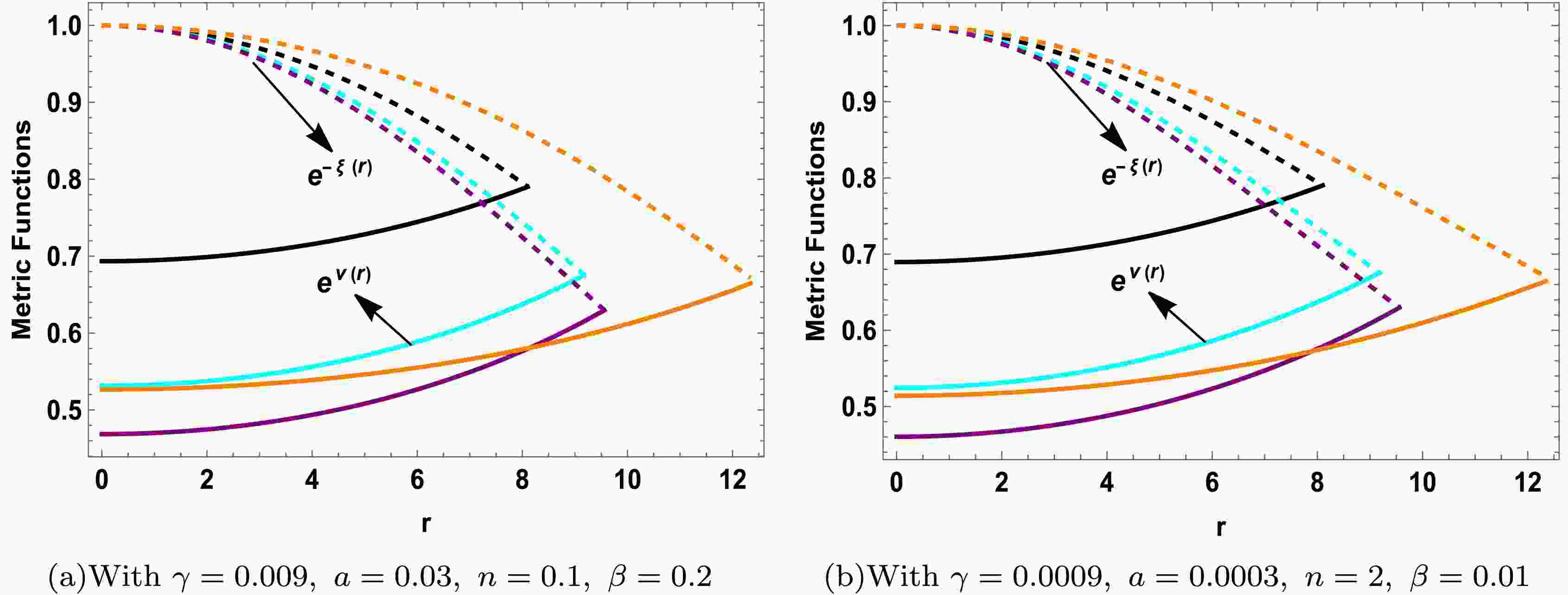
$ \begin{aligned} {\rm e}^{\nu(r)}&=\left(\mathbb{A}+\frac{\mathbb{B} \sqrt{cr^2 {\rm e}^{a n r^2}}}{a n r}\right)^2, \end{aligned} $

(38) $ \begin{aligned} {\rm e}^{-\xi(r)}&=\frac{(1+cr^2 {\rm e}^{nar^2})(cr^2+1)}{(cr^2+1)+\beta ncr^2(1+cr^2{\rm e}^{nar^2})}. \end{aligned} $

(39) In subsequent computations, the characterization of the total state quantities, that is, the energy density and the radial and tangential pressures will be implemented, as follows:
$ \begin{aligned} \rho^{({\rm{total}})}&=\rho+\alpha\vartheta^{0}_{0}, \end{aligned} $

(40) $ \begin{aligned} p^{({\rm{total}})}_{r}&=p_r-\alpha\vartheta^{1}_{1}, \end{aligned} $

(41) $ \begin{aligned} p^{({\rm{total}})}_t&=p_t-\alpha\vartheta^{2}_{2}, \end{aligned} $

(42) where density and pressure are given by Eqs. (21)−(23). These relations involve additional geometric quantities that interact via the coupling parameter α.
The quantities
$ \rho^{({\rm{total}})} $ , along with$ p^{({\rm{total}})}_{r} $ and$ p^{({\rm{total}})}_{t} $ for completing the system, are expressed as follows:$ \begin{aligned}[b] \rho^{\rm{total}}=\;&\frac{1}{3 k_1 r^2 \left(2\gamma+k_1\right)}\Bigg(\frac{1}{k_2 r+1}\Bigg(\frac{4 {\rm{a}}^2 \mathbb{B}^2 \gamma k_2^2 n^2 r^4}{k_3^2}+\frac{4 {\rm{a}} \mathbb{B} \gamma n \left(k_2 r\right){}^{3/2} \left({\rm{a}}\mathbb{A} n r \left({\rm{a}} n r^2+1\right)+\mathbb{B} \sqrt{k_2 r}\right)}{k_3^2}\\ &+\frac{2{\rm{a}}\mathbb{B}\gamma k_2n r^2\left(\dfrac{2{\rm{a}}nr^2+2}{k_2 r+1}-2{\rm{a}}n r^2+2\right)}{k_3} +\frac{4 k_2 r \left({\rm{a}} n r^2+1\right) (8\gamma+48\pi G+3\lambda)}{k_2 r+1}+2k_2r(8\gamma+48\pi G+3\lambda)\Bigg)\\ &+\frac{2\beta{\rm{c}}nr^2}{\left({\rm{c}}r^2+1\right)^2}\Bigg(\bigg(k_2\big(-{\rm{a}}^2 \mathbb{A}^2 n^2r(8\gamma+3\lambda) \left({\rm{c}}r^2+3\right)+2{\rm{a}}\mathbb{A}\mathbb{B}n\sqrt{k_2 r}\big(\gamma\big(r^2 \big({\rm{c}}\left({\rm{a}}n r^2\left({\rm{a}} n r^2+3\right)-8\right)\\ &+{\rm{a}} n \left({\rm{a}}n r^2+4\right)\big)-24\big)-3 \lambda \left({\rm{c}} r^2+3\right)\big)+\mathbb{B}^2k_2\big(2\gamma\big(r^2 \left({\rm{a}} n r^2+4\right) \big({\rm{a}} {\rm{c}} n r^2\\ &+{\rm{a}} n-{\rm{c}}\big)-12\big)-3\lambda\left({\rm{c}} r^2+3\right)\big)\big)\bigg/(k_3^2)+48 \pi G\left({\rm{c}}r^2+3\right)\Bigg)\Bigg), \\ p_r^{\rm{total}}=\;&\frac{1}{3 k_1 r^2\left(2\gamma+k_1\right)}\Bigg(\frac{1}{k_2 r+1}\Bigg(-\frac{4{\rm{a}}^2\mathbb{B}^2 \gamma k_2^2 n^2 r^4}{k_3^2}-\frac{4{\rm{a}}\mathbb{B}\gamma n\left(k_2r\right){}^{3/2} \left({\rm{a}}\mathbb{A}nr\left({\rm{a}} n r^2+1\right)+\mathbb{B}\sqrt{k_2 r}\right)}{k_3^2}\\ &+\frac{2{\rm{a}}\mathbb{B}k_2 n r^2 \left(2\gamma\left(-\dfrac{{\rm{a}}nr^2+1}{k_2 r+1}+{\rm{a}}nr^2+11\right)+96\pi G+6\lambda \right)}{k_3}+\frac{16\gamma k_2 r\left({\rm{a}}nr^2+1\right)}{k_2 r+1}-2 k_2 r (8 \gamma \\ &+48\pi G+3\lambda)\Bigg)+\Bigg(\beta{\rm{c}} n r^2 \big(\Bigg(2 \big({\rm{a}}\mathbb{A}n\left({\rm{c}}r^2+1\right) \sqrt{k_2 r}(8\gamma+48\pi G+3\lambda)+\mathbb{B}k_2 \big(48\pi G\left({\rm{c}}r^2+1\right)\left(2{\rm{a}}n r^2+1\right)\\ &+2\gamma \left(r^2\left({\rm{c}}\left({\rm{a}} n r^2 \big(9-{\rm{a}} n r^2\big)+4\right)+{\rm{a}}n\left(8-{\rm{a}}nr^2\right)\right) +4\right)+3\lambda\left({\rm{c}} r^2+1\right) \left(2 {\rm{a}} n r^2+1\right)\big)\big)\Big)/(k_3)-16 \gamma \big)\Bigg)\\ &\Bigg/\Bigg(\left({\rm{c}} r^2+1\right)^2\Bigg)\Bigg),\\ p_t^{\rm{total}}=\;&\frac{{\rm{c}}}{3 k_1\left(2\gamma+k_1\right)}\Bigg(\Bigg(2 r {\rm e}^{{\rm{a}} n r^2} \bigg ({\rm{a}}^2\mathbb{A}^2 k_2 n^2 \left(-48 G \left(\pi{\rm{a}}nr^2+\pi\right)+r^2\left(\frac{4\gamma k_2}{r} -{\rm{a}}n(4\gamma+3\lambda)\right)-3 \lambda \right)\\ &+{\rm{a}}\mathbb{B}n\sqrt{k_2 r}\left(-3 (16 \pi G+\lambda )k_{\frac{2}{r}} \left({\rm{a}} n r^2+2\right)+{\rm{a}} n \left(48 \pi G \left({\rm{a}} n r^2+2\right)+{\rm{a}} n r^2 (10 \gamma +3 \lambda )+6 (3 \gamma +\lambda )\right)+8 \gamma k_2^2\right)\\ &+\mathbb{B}^2 k_2 \left(\frac{k_2\left(4{\rm{a}}\gamma nr^2-48\pi G-3\lambda\right)}{r}+{\rm{a}}n\left(48\pi G \left({\rm{a}} n r^2+2\right)+{\rm{a}} n r^2 (10 \gamma +3 \lambda )+6 (3 \gamma +\lambda )\right)+4 \gamma k_2^2\right)\bigg)\\ &\Bigg/({k_3^2 \left(k_2 r+1\right){}^2}\Bigg)+\Bigg(\beta n \bigg(\Bigg(2 k_2 \left({\rm{c}} r^2+1\right) \bigg ({\rm{a}}^3 \mathbb{A}\mathbb{B} n^3 r^4 \sqrt{k_2 r} (10 \gamma +48 \pi G+3 \lambda )+{\rm{a}}^2 n^2r\bigg(-4\mathbb{A}^2 \gamma \\&+6 \mathbb{A}\mathbb{B} r \sqrt{k_2 r} (3 \gamma +16 \pi G+\lambda )+\mathbb{B}^2 k_2 r^3 (10 \gamma +48 \pi G+3 \lambda )\bigg)+2 {\rm{a}}\mathbb{B}n\left(3\mathbb{B} k_2 r^2 (3\gamma+16 \pi G+\lambda) -4\mathbb{A}\gamma\sqrt{k_2 r}\right)\\ &-4\mathbb{B}^2 \gamma k_2\bigg)\Bigg)\Bigg/\Bigg(k_3^2\Bigg)+\frac{2{\rm{a}}\mathbb{B}k_2 n r^2 (10\gamma+48\pi G+3\lambda)}{k_3}+8\gamma+96\pi G+6\lambda\bigg)\Bigg)\Bigg/\Bigg(\left({\rm{c}}r^2+1\right)^2\Bigg)\Bigg), \end{aligned} $

(43) where
$ \begin{aligned} k_1=s2 \gamma +16 \pi G+\lambda, \quad k_2={\rm{c}}r {\rm e}^{{\rm{a}} n r^2}, \quad k_3={\rm{a}}\mathbb{A} n \sqrt{k_2 r}+\mathbb{B}k_2. \end{aligned} $

-
To solve the two sets of field equations involving unknown functions
$ W(r) $ and$ H(r) $ , we select a metric potential that meets the key criteria: it must be finite, monotonically increasing with r, and reach a minimum at$ r = 0 $ , ensuring regularity. These conditions, as outlined in [63], are essential for deriving physically viable static spherically symmetric perfect fluid solutions. In this work, we adopt the following form for the metric potential, which satisfies the necessary mathematical conditions and facilitates the derivation of physically viable expressions for the effective energy density and pressures. The chosen metric potential is given by$ \begin{aligned} e^{W}=1+ c r^2e^{n a r^2}, \end{aligned} $
(30) where c, n, and a are arbitrary constants. This specific form has been widely utilized as an ansatz, particularly in the construction of class-I solutions [64, 65]. It is interesting to mention here that this metric is consistent with the criteria of being regular at the center, exhibiting monotonically increasing trend with minimum at
$ r=0 $ , and$ e^W=1+O(r^2) $ . Therefore, it is a valid choice to consider for modeling of compact stars within this theory. For a spacetime to be categorized under embedding class-I, it is imperative that Eq.(25) satisfies the Karmarkar condition, originally formulated by Karmarkar in 1948 [66]. This condition is expressed as$ \begin{aligned} {\cal{R}}_{1414}=\frac{{\cal{R}}_{1212}{\cal{R}}_{3434}+{\cal{R}}_{1224}{\cal{R}}_{1334}}{{\cal{R}}_{2323}}. \end{aligned} $
(31) By incorporating the condition specified in Eq.(31), and given that
$ R_{2323} \neq 0 $ as noted in [67], we derive the following equation that establishes a relationship between the two spacetime functions$ W(r) $ and$ H(r) $ , as outlined below$ \begin{aligned} \frac{W^{\prime}H^{\prime}}{1-e^{W}}=W^{\prime}H^{\prime}-2H^{\prime \prime}-H^{\prime 2}, \end{aligned} $
(32) where
$ e^{W(r)} \neq 1 $ . By integrating the first equation, we derive the subsequent equation, which illustrates the manner in which the four-dimensional spacetime, as described by Eq.(31), is embedded within a five-dimensional pseudo-Euclidean space. This corresponds to solutions of embedding class-I. It is defined as$ \begin{aligned} e^{H(r)}=\Bigg(\mathbb{A}+\mathbb{B} \int \sqrt{e^{ W(r)}-1} \,dr \Bigg)^2, \end{aligned} $
(33) where
$ \mathbb{A} $ and$ \mathbb{B} $ are constants due to integration. Substituting Eq.(30) into the above equation permits us to determine the value of the metric$ e^{H(r)} $ , as provided below$ \begin{aligned} e^{H(r)}=\left(\mathbb{A}+\frac{\mathbb{B}\sqrt{cr^2 e^{a n r^2}}}{a n r}\right)^2. \end{aligned} $
(34) The constants
$ \mathbb{A} $ ,$ \mathbb{B} $ , and c can be evaluated through the application of the matching condition. In the subsequent section, we will fix the constants λ and a. It is noted that the metric potential$ e^{H(r)} $ is a radial dependent monotonically increasing function and exhibits positive, finite, and regular trend with$ e^{H(r)} \to 1 $ as$ r \to 0 $ , thus ensuring the absence of singularities. Therefore, this metric potential is suitable for modeling a relativistic compact object within the framework of$ f({\cal{R}},T,{\cal{L}}_m) $ gravity via MGD approach. Below line element can then be used to describe the field equations given by Eqs.(21) through (23):$ \begin{aligned}[b] ds^2=\;&-\Bigg(\mathbb{A}+\frac{\mathbb{B} \sqrt{cr^2 e^{a n r^2}}}{a n r}\Bigg)^2 dt^2+\Bigg(1+ c r^2e^{nar^2}\Bigg)^{-1}dr^2\\&+r^2\Big(d\theta^2+\sin^2{\theta}d\phi^2\Big). \end{aligned} $
(35) To obtain the complete solutions for our model, it is necessary to calculate the components of
$ \vartheta_{\mu\nu} $ . This requires determining the deformation function$ \psi(r) $ . Several methods can be employed to find$ \psi(r) $ , including:● Mimicking the density constraint (
$ \vartheta_0^0=\rho $ );● Mimicking the pressure constraint (
$ \vartheta_1^1 = p_r $ );● Relating the components of
$ \vartheta_{\mu \nu} $ through various equations of state, such as polytropic, barotropic, or linear equations.However, the determination of deformation function
$ \psi(r) $ often becomes mathematically intricate, especially when aiming to maintain physical acceptability and analytic solvability. To address this, we adopt a deformation function that is free from singularities, exhibits a non-decreasing behavior, and has been extensively utilized in previous studies for constructing physically viable anisotropic models [68−70]. The chosen form is not arbitrary; it is carefully selected to be fully compatible with the prescribed seed solution, ensuring that the resulting field equations remain analytically tractable and physically consistent. While alternative functional forms for$ \psi(r) $ are theoretically permissible, they frequently introduce significant non-linearities or yield unphysical features, such as singularities or negative pressures. Moreover, the selected function has also been successfully employed in conjunction with the same seed metric in earlier works, further justifying its use in the present analysis. This form is given by$ \begin{aligned} \psi(r)=\frac{ncr^2}{cr^2+1}. \end{aligned} $
(36) The complete spacetime structure related to the energy-momentum tensor
$ T^{eff}_{\mu \nu} $ can be explicitly defined as follows$ \begin{aligned}[b] ds^2=\;&-\Bigg(\mathbb{A}+\frac{\mathbb{B}\sqrt{cr^2 e^{a n r^2}}}{a n r}\Bigg)^2 dt^2 \\&+\Bigg(\frac{(1+cr^2 e^{nar^2})(cr^2+1)}{(cr^2+1)+\beta ncr^2(1+cr^2e^{nar^2})}\Bigg)dr^2 \\&+r^2\Big(d\theta^2+\sin^2{\theta}d\phi^2\Big), \end{aligned} $
(37) where
$ \begin{aligned} e^{\nu(r)}&=\left(\mathbb{A}+\frac{\mathbb{B} \sqrt{cr^2 e^{a n r^2}}}{a n r}\right)^2, \end{aligned} $
(38) $ \begin{aligned} e^{-\xi(r)}&=\frac{(1+cr^2 e^{nar^2})(cr^2+1)}{(cr^2+1)+\beta ncr^2(1+cr^2e^{nar^2})}. \end{aligned} $
(39) In the subsequent computations, below characterization of total state quantities, i.e., the energy density, radial and tangential pressures will be implemented:
$ \begin{aligned} \rho^{({\rm{total}})}&=\rho+\alpha\vartheta^{0}_{0}, \end{aligned} $
(40) $ \begin{aligned} p^{({\rm{total}})}_{r}&=p_r-\alpha\vartheta^{1}_{1}, \end{aligned} $
(41) $ \begin{aligned} p^{({\rm{total}})}_t&=p_t-\alpha\vartheta^{2}_{2}, \end{aligned} $
(42) where density and pressures are provided by Eqs.(21)-(23). These relations involve additional geometric quantities which are interacted via coupling parameter α.
The quantities
$ \rho^{({\rm{total}})} $ , along with$ p^{({\rm{total}})}_{r} $ and$ p^{({\rm{total}})}_{t} $ for completing the system, can be expressed as follows$ \begin{aligned}[b] \rho^{total}=\;&\frac{1}{3 k_1 r^2 \left(2\gamma+k_1\right)}\Bigg(\frac{1}{k_2 r+1}\Bigg(\frac{4 {\rm{a}}^2 \mathbb{B}^2 \gamma k_2^2 n^2 r^4}{k_3^2}+\frac{4 {\rm{a}} \mathbb{B} \gamma n \left(k_2 r\right){}^{3/2} \left({\rm{a}}\mathbb{A} n r \left({\rm{a}} n r^2+1\right)+\mathbb{B} \sqrt{k_2 r}\right)}{k_3^2}\\ &+\frac{2{\rm{a}}\mathbb{B}\gamma k_2n r^2\left(\dfrac{2{\rm{a}}nr^2+2}{k_2 r+1}-2{\rm{a}}n r^2+2\right)}{k_3} +\frac{4 k_2 r \left({\rm{a}} n r^2+1\right) (8\gamma+48\pi G+3\lambda)}{k_2 r+1}+2k_2r(8\gamma+48\pi G+3\lambda)\Bigg)\\ &+\frac{2\beta{\rm{c}}nr^2}{\left({\rm{c}}r^2+1\right)^2}\Bigg(\bigg(k_2\big(-{\rm{a}}^2 \mathbb{A}^2 n^2r(8\gamma+3\lambda) \left({\rm{c}}r^2+3\right)+2{\rm{a}}\mathbb{A}\mathbb{B}n\sqrt{k_2 r}\big(\gamma\big(r^2 \big({\rm{c}}\left({\rm{a}}n r^2\left({\rm{a}} n r^2+3\right)-8\right)\\ &+{\rm{a}} n \left({\rm{a}}n r^2+4\right)\big)-24\big)-3 \lambda \left({\rm{c}} r^2+3\right)\big)+\mathbb{B}^2k_2\big(2\gamma\big(r^2 \left({\rm{a}} n r^2+4\right) \big({\rm{a}} {\rm{c}} n r^2\\ &+{\rm{a}} n-{\rm{c}}\big)-12\big)-3\lambda\left({\rm{c}} r^2+3\right)\big)\big)\bigg/(k_3^2)+48 \pi G\left({\rm{c}}r^2+3\right)\Bigg)\Bigg), \\ p_r^{total}=\;&\frac{1}{3 k_1 r^2\left(2\gamma+k_1\right)}\Bigg(\frac{1}{k_2 r+1}\Bigg(-\frac{4{\rm{a}}^2\mathbb{B}^2 \gamma k_2^2 n^2 r^4}{k_3^2}-\frac{4{\rm{a}}\mathbb{B}\gamma n\left(k_2r\right){}^{3/2} \left({\rm{a}}\mathbb{A}nr\left({\rm{a}} n r^2+1\right)+\mathbb{B}\sqrt{k_2 r}\right)}{k_3^2}\\ &+\frac{2{\rm{a}}\mathbb{B}k_2 n r^2 \left(2\gamma\left(-\dfrac{{\rm{a}}nr^2+1}{k_2 r+1}+{\rm{a}}nr^2+11\right)+96\pi G+6\lambda \right)}{k_3}+\frac{16\gamma k_2 r\left({\rm{a}}nr^2+1\right)}{k_2 r+1}-2 k_2 r (8 \gamma \\ &+48\pi G+3\lambda)\Bigg)+\Bigg(\beta{\rm{c}} n r^2 \big(\Bigg(2 \big({\rm{a}}\mathbb{A}n\left({\rm{c}}r^2+1\right) \sqrt{k_2 r}(8\gamma+48\pi G+3\lambda)+\mathbb{B}k_2 \big(48\pi G\left({\rm{c}}r^2+1\right)\left(2{\rm{a}}n r^2+1\right)\\ &+2\gamma \left(r^2\left({\rm{c}}\left({\rm{a}} n r^2 \big(9-{\rm{a}} n r^2\big)+4\right)+{\rm{a}}n\left(8-{\rm{a}}nr^2\right)\right) +4\right)+3\lambda\left({\rm{c}} r^2+1\right) \left(2 {\rm{a}} n r^2+1\right)\big)\big)\Big)/(k_3)-16 \gamma \big)\Bigg)\\ &\Bigg/\Bigg(\left({\rm{c}} r^2+1\right)^2\Bigg)\Bigg),\\ p_t^{total}=\;&\frac{{\rm{c}}}{3 k_1\left(2\gamma+k_1\right)}\Bigg(\Bigg(2 r e^{{\rm{a}} n r^2} \bigg ({\rm{a}}^2\mathbb{A}^2 k_2 n^2 \left(-48 G \left(\pi{\rm{a}}nr^2+\pi\right)+r^2\left(\frac{4\gamma k_2}{r} -{\rm{a}}n(4\gamma+3\lambda)\right)-3 \lambda \right)\\ &+{\rm{a}}\mathbb{B}n\sqrt{k_2 r}\left(-3 (16 \pi G+\lambda )k_{\frac{2}{r}} \left({\rm{a}} n r^2+2\right)+{\rm{a}} n \left(48 \pi G \left({\rm{a}} n r^2+2\right)+{\rm{a}} n r^2 (10 \gamma +3 \lambda )+6 (3 \gamma +\lambda )\right)+8 \gamma k_2^2\right)\\ &+\mathbb{B}^2 k_2 \left(\frac{k_2\left(4{\rm{a}}\gamma nr^2-48\pi G-3\lambda\right)}{r}+{\rm{a}}n\left(48\pi G \left({\rm{a}} n r^2+2\right)+{\rm{a}} n r^2 (10 \gamma +3 \lambda )+6 (3 \gamma +\lambda )\right)+4 \gamma k_2^2\right)\bigg)\\ &\Bigg/({k_3^2 \left(k_2 r+1\right){}^2}\Bigg)+\Bigg(\beta n \bigg(\Bigg(2 k_2 \left({\rm{c}} r^2+1\right) \bigg ({\rm{a}}^3 \mathbb{A}\mathbb{B} n^3 r^4 \sqrt{k_2 r} (10 \gamma +48 \pi G+3 \lambda )+{\rm{a}}^2 n^2r\bigg(-4\mathbb{A}^2 \gamma \\&+6 \mathbb{A}\mathbb{B} r \sqrt{k_2 r} (3 \gamma +16 \pi G+\lambda )+\mathbb{B}^2 k_2 r^3 (10 \gamma +48 \pi G+3 \lambda )\bigg)+2 {\rm{a}}\mathbb{B}n\left(3\mathbb{B} k_2 r^2 (3\gamma+16 \pi G+\lambda) -4\mathbb{A}\gamma\sqrt{k_2 r}\right)\\ &-4\mathbb{B}^2 \gamma k_2\bigg)\Bigg)\Bigg/\Bigg(k_3^2\Bigg)+\frac{2{\rm{a}}\mathbb{B}k_2 n r^2 (10\gamma+48\pi G+3\lambda)}{k_3}+8\gamma+96\pi G+6\lambda\bigg)\Bigg)\Bigg/\Bigg(\left({\rm{c}}r^2+1\right)^2\Bigg)\Bigg), \end{aligned} $
(43) where
$ \begin{aligned} k_1=s2 \gamma +16 \pi G+\lambda, \quad k_2={\rm{c}}r e^{{\rm{a}} n r^2}, \quad k_3={\rm{a}}\mathbb{A} n \sqrt{k_2 r}+\mathbb{B}k_2. \end{aligned} $
-
Matching conditions are crucial for understanding the physical characteristics of any gravitational model by aligning interior and exterior geometries across a hypersurface. This process is governed by two primary conditions:
● Continuity of metric coefficients: The metric components of both spacetimes must be continuous at the hypersurface. This constraint ensures that there is no discontinuity in the metrics across the boundary.
● Extrinsic curvature matching: The extrinsic curvatures of both spacetimes must be equal at the hypersurface. This requirement leads to the condition
$ p_r^{{\rm{eff}}} = 0 $ , which implies that there is no difference in the tensor components of the stress energy across the boundary.These conditions are essential for ensuring smooth transition and consistency across the interior and exterior geometries of any gravitational model. For this study, we selected the exterior Schwarzschild spacetime as follows:
$ \begin{aligned}[b] {\rm d}s^2=\;&-\Bigg(1-\frac{2{\cal{M}}}{r}\Bigg){\rm d}t^2+\Bigg(1-\frac{2{\cal{M}}}{r}\Bigg)^{-1}{\rm d}r^2 \\&+r^2\Big({\rm d}\theta^2+\sin^2{\theta}{\rm d}\phi^2\Big). \end{aligned} $

(44) By equating the exterior spacetime metric with Eq. (37) and applying the continuity conditions for the metric potentials, we derive the following two relations:
$ \begin{aligned} {\rm e}^{v(r)}&=1-\frac{2{\cal{M}}}{{\cal{R}}} , \end{aligned} $

(45) $ \begin{aligned} {\rm e}^{-\xi(r)}&=1-\frac{2{\cal{M}}}{{\cal{R}}}, \end{aligned} $

(46) where the terms
$ {\cal{M}} $ and$ {\cal{R}} $ refer to the total mass and radius of the compact star, respectively. The second form of continuity, in which the pressure vanishes at the boundary and hence allows stability in a true vacuum, is presented as follows:$ \begin{aligned} p_r^{\rm total}(r)|_{r={\cal{R}}}=\Bigg(p_r-\alpha \vartheta^1_1\Bigg)|_{r={\cal{R}}}=0. \end{aligned} $

(47) By utilizing Eqs. (45)−(47) and re-arranging them with the appropriate substitutions, the values of the random constants
$ \mathbb{A} $ ,$ \mathbb{B} $ , and c can be obtained as follows:$ \begin{aligned}[b] \mathbb{A}=\;&-\frac{{\rm{B}}\sqrt{{\rm{c}}{\cal{R}}^2 {\rm e}^{{\rm{a}}n*{\cal{R}}^2}}+{\rm{a}}n\sqrt{{\cal{R}}} \sqrt{{\cal{R}}-2{\cal{M}}}}{{\rm{a}}n{\cal{R}}},\\ \mathbb{B}=\;&\Bigg(\Big({\rm{c}}\sqrt{{\cal{R}}}\sqrt{{\cal{R}}-2 {\cal{M}}}\big({\rm{c}}{\cal{R}}^2{\rm e}^{2{\rm{a}}n {\cal{R}}^2}\big(8\gamma\left(\beta{\rm{c}}^2n{\cal{R}}^4 -\left({\rm{c}}{\cal{R}}^2+1\right)^2\right)+48\pi G\left({\rm{c}}{\cal{R}}^2+1\right)\left({\rm{c}}{\cal{R}}^2(\beta n-1)-1\right)\\ &+3\lambda\left({\rm{c}}{\cal{R}}^2+1\right)\left({\rm{c}}{\cal{R}}^2(\beta n-1)-1\right)\big)+{\rm e}^{{\rm{a}}n{\cal{R}}^2}\big(8{\rm{a}}\gamma n\left({\rm{c}} {\cal{R}}^3+{\cal{R}}\right)^2+16\beta\gamma{\rm{c}}^2 n {\cal{R}}^4+48\pi G\left({\rm{c}}{\cal{R}}^2+1\right)\\ &*\left({\rm{c}}{\cal{R}}^2(2\beta n-1)-1\right)+3\lambda\left({\rm{c}}{\cal{R}}^2+1\right)\left({\rm{c}}{\cal{R}}^2(2\beta n-1) -1\right)\big)+\beta n\left(48G\left(\pi{\rm{c}}{\cal{R}}^2+\pi\right)+{\rm{c}}{\cal{R}}^2(8\gamma+3\lambda) +3\lambda\right)\big)\Big)\\ &/\Big(2\sqrt{{\rm{c}}{\cal{R}}^2{\rm e}^{{\rm{a}}n{\cal{R}}^2}}\big(\gamma\big({\cal{R}}^2\big({\rm{c}}\big(\beta{\rm{c}}^2n{\cal{R}}^4{\rm e}^{2{\rm{a}}n{\cal{R}}^2} \left({\cal{R}}^2 \left({\rm{c}} \left({\rm{a}} n {\cal{R}}^2-9\right)+{\rm{a}} n\right)-8\right)+{\rm{c}} {\cal{R}}^2 (\beta n+1) \left({\rm{a}} n {\cal{R}}^2-9\right)\\ &+2 {\rm e}^{{\rm{a}} n {\cal{R}}^2} \left(\beta {\rm{c}} n {\cal{R}}^2 \left({\cal{R}}^2 \left({\rm{c}} \left({\rm{a}} n {\cal{R}}^2-9\right)+{\rm{a}} n\right)-8\right)-5 \left({\rm{c}} {\cal{R}}^2+1\right)^2\right)+{\rm{a}} n {\cal{R}}^2 (\beta n+2)-8\beta n-18\big)+{\rm{a}} n\big)-9\big)\\ &-48 \pi G \left({\rm{c}}{\cal{R}}^2+1\right) \left({\rm{c}} {\cal{R}}^2 {\rm e}^{{\rm{a}} n {\cal{R}}^2}+1\right) \left({\rm{c}}{\cal{R}}^2 \left(\beta n \left({\rm{c}} {\cal{R}}^2 {\rm e}^{{\rm{a}} n {\cal{R}}^2}+1\right)+1\right)+1\right)-3 \lambda\left({\rm{c}} {\cal{R}}^2+1\right)\\ &*\left({\rm{c}} {\cal{R}}^2 {\rm e}^{{\rm{a}} n {\cal{R}}^2}+1\right) \left({\rm{c}} {\cal{R}}^2 \left(\beta n \left({\rm{c}}{\cal{R}}^2 {\rm e}^{{\rm{a}} n {\cal{R}}^2}+1\right)+1\right)+1\right)\big)\Big)\Bigg),\\ c=\;&\Bigg(4 {\cal{M}}\Bigg)/\Bigg(-2 {\cal{M}} {\cal{R}}^2 \left({\rm e}^{{\rm{a}} n {\cal{R}}^2}+1\right)+\sqrt{{\cal{R}}^4 \left(\left(-({\cal{R}}-2 {\cal{M}}) {\rm e}^{{\rm{a}} n {\cal{R}}^2}+2 {\cal{M}}+\beta n {\cal{R}}\right)^2-8 {\cal{M}} {\rm e}^{{\rm{a}} n {\cal{R}}^2} (2 {\cal{M}}+{\cal{R}} (\beta n-1))\right)}\\ &+{\cal{R}}^3 \left({\rm e}^{{\rm{a}} n {\cal{R}}^2}-\beta n\right)\Bigg). \end{aligned} $

(48) Random constants
$ \mathbb{A} $ ,$ \mathbb{B} $ , and c are then evaluated by taking$ \beta = 0.2 $ and$ \beta = -0.2 $ , and the summary of resulting values is provided in Tables 1 and 2, in which the data of seven selected stellar models has been utilized. In both instances, the fixed parameters are$ \lambda = 1 \times 10^{-12} $ ,$ a = 0.03 $ , and$ \gamma = 0.009 $ , whereas the coupling parameter can assume any non-zero real value, as illustrated in the tables.Star Models Mass $ {\cal{M}}/{\cal{M}}_{\odot} $ 

Radius $ {\cal{R}} $ (km)

Mass-radius( $ \frac{{\cal{M}}}{{\cal{R}}} $ )

c $ \mathbb{B} $ 

$ \mathbb{A} $ 

Her X-1 [69] 0.85±0.15 8.1±0.41 0.154 0.00339865 −0.0279575 −0.289412 LMC X-4 [70] 1.04±0.09 8.301±0.2 0.184 0.00403809 −0.029791 −0.165948 Cen X-3 [71] 1.49±0.08 9.178±0.13 0.239 0.00454612 −0.0306402 −0.0403881 4U 1608-52 [72] 1.74±0.14 9.528±0.15 0.269 0.0049576 −0.03128 0.0445229 Vela X-1 1.77±0.08 9.56±0.08 0.273 0.00502456 −0.0312868 0.057035 PSR J1614-2230 [73] 1.97±0.04 9.69±0.2 0.300 0.0056665 −0.0324197 0.166191 PSR J0740+6620 [74] 2.07±0.04 12.34±0.2 0.247 0.00214646 −0.02322001 −0.3364949 Table 1. Synopsis of computed values of constants based on the data of seven stellar candidates for MGD case (
$ \beta=0.2, \; \lambda=1*10^{-12}, $ $ a=0.03, \; \gamma=0.009 $ ).Star Models Mass $ {\cal{M}}/{\cal{M}}_{\odot} $ 

Radius $ {\cal{R}} $ (km)

Mass-radius( $ \frac{{\cal{M}}}{{\cal{R}}} $ )

c $ \mathbb{B} $ 

$ \mathbb{A} $ 

Her X-1 [69] 0.85±0.15 8.1±0.41 0.154 0.00325493 −0.028568 −0.289414 LMC X-4 [70] 1.04±0.09 8.301±0.2 0.184 0.0038583 −0.0304771 −0.165951 Cen X-3 [71] 1.49±0.08 9.178±0.13 0.239 0.00432607 −0.0314096 −0.0403919 4U 1608-52 [72] 1.74±0.14 9.528±0.15 0.269 0.00470364 −0.0321131 0.0445179 Vela X-1 1.77±0.08 9.56±0.08 0.273 0.00476514 −0.0322297 0.0570297 PSR J1614-2230 [73] 1.97±0.04 9.69±0.2 0.300 0.00535511 −0.0333488 0.166184 PSR J0740+6620 [74] 2.07±0.04 12.34±0.2 0.247 0.00205513 −0.0237099 −0.364951 Table 2. Synopsis of computed values of constants based on the data of seven star models for MGD case (
$ \beta=-0.2, \; \lambda=1*10^{-12}, $ $ a=0.03, \; \gamma=0.009 $ ).Utilizing the listed constant values for the selected stellar candidates, we generated plots of the metric potentials, as shown in Figs. 1(a) and 1(b). These figures illustrate the trend of the metric potentials as functions of the radial coordinate r for two distinct constant values across the four stellar models. In both cases, the metric potentials exhibit regular, monotonically increasing, and finite behavior throughout the stellar interior, without any indication of singularities.
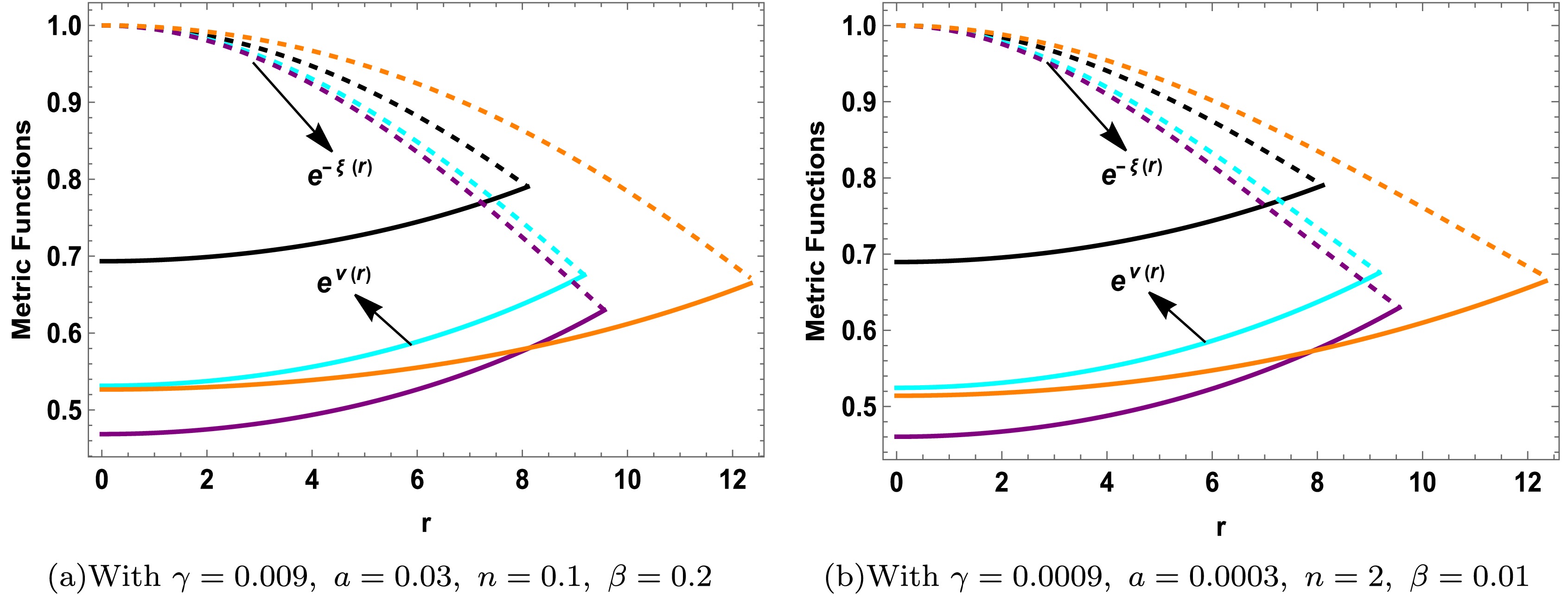
Figure 1. (color online) For the compact star Her X-1 (
$ {\cal{M}}/{\cal{M}}_{\odot}=0.85 $ ,$ {\cal{R}}=8.1 $ )(■), Cen X-3 ($ {\cal{M}}/{\cal{M}}_{\odot}=1.49 $ ,$ {\cal{R}}= 9.178 $ )(■), Vela X-1 ($ {\cal{M}}/{\cal{M}}_{\odot}=1.77 $ ,$ {\cal{R}}=9.56 $ )(■) and PSR J0740+6620 ($ {\cal{M}}/{\cal{M}}_{\odot}=2.07 $ ,$ {\cal{R}} =12.34 $ )(■), the variations in metric functions against r are shown. All plots use$ \lambda=1 \times 10^{-12} $ . -
Matching conditions are crucial for understanding the physical characteristics of any gravitational model by aligning the interior and exterior geometries across a hypersurface. This process is governed by two primary conditions:
● Continuity of metric coefficients: The metric components of both spacetimes must be continuous at the hypersurface. This constraint ensures that there is no discontinuity in the metric across the boundary.
● Extrinsic curvature matching: The extrinsic curvature of both spacetimes must be equal at the hypersurface. This requirement, further, leads to the condition:
$ p_r^{{\rm{eff}}} = 0 $ , which means that there is no difference in the tensor components of the stress energy across the boundary.These conditions are essential for ensuring a smooth transition and consistency across the interior and exterior geometries of any gravitational model. For this study, we choose the exterior Schwarzschild spacetime as given below
$ \begin{aligned}[b] ds^2=\;&-\Bigg(1-\frac{2{\cal{M}}}{r}\Bigg)dt^2+\Bigg(1-\frac{2{\cal{M}}}{r}\Bigg)^{-1}dr^2 \\&+r^2\Big(d\theta^2+\sin^2{\theta}d\phi^2\Big). \end{aligned} $
(44) By equating the above exterior spacetime metric with Eq.(37) and applying the continuity conditions for the metric potentials, we derive the following two relations:
$ \begin{aligned} e^{v(r)}&=1-\frac{2{\cal{M}}}{{\cal{R}}} , \end{aligned} $
(45) $ \begin{aligned} e^{-\xi(r)}&=1-\frac{2{\cal{M}}}{{\cal{R}}}, \end{aligned} $
(46) where the terms
$ {\cal{M}} $ and$ {\cal{R}} $ , respectively, refer to total mass and radius of the compact star. The second form of continuity, in which the pressure vanishes at the boundary and hence allows stability in a true vacuum, is presented below:$ \begin{aligned} p_r^{total}(r)|_{r={\cal{R}}}=\Bigg(p_r-\alpha \vartheta^1_1\Bigg)|_{r={\cal{R}}}=0. \end{aligned} $
(47) By utilizing Eqs.(45)-(47) and re-arranging them with the appropriate substitutions, the values of the random constants
$ \mathbb{A} $ ,$ \mathbb{B} $ , and c can be found as follows$ \begin{aligned}[b] \mathbb{A}=\;&-\frac{{\rm{B}}\sqrt{{\rm{c}}{\cal{R}}^2 e^{{\rm{a}}n*{\cal{R}}^2}}+{\rm{a}}n\sqrt{{\cal{R}}} \sqrt{{\cal{R}}-2{\cal{M}}}}{{\rm{a}}n{\cal{R}}},\\ \mathbb{B}=\;&\Bigg(\Big({\rm{c}}\sqrt{{\cal{R}}}\sqrt{{\cal{R}}-2 {\cal{M}}}\big({\rm{c}}{\cal{R}}^2e^{2{\rm{a}}n {\cal{R}}^2}\big(8\gamma\left(\beta{\rm{c}}^2n{\cal{R}}^4 -\left({\rm{c}}{\cal{R}}^2+1\right)^2\right)+48\pi G\left({\rm{c}}{\cal{R}}^2+1\right)\left({\rm{c}}{\cal{R}}^2(\beta n-1)-1\right)\\ &+3\lambda\left({\rm{c}}{\cal{R}}^2+1\right)\left({\rm{c}}{\cal{R}}^2(\beta n-1)-1\right)\big)+e^{{\rm{a}}n{\cal{R}}^2}\big(8{\rm{a}}\gamma n\left({\rm{c}} {\cal{R}}^3+{\cal{R}}\right)^2+16\beta\gamma{\rm{c}}^2 n {\cal{R}}^4+48\pi G\left({\rm{c}}{\cal{R}}^2+1\right)\\ &*\left({\rm{c}}{\cal{R}}^2(2\beta n-1)-1\right)+3\lambda\left({\rm{c}}{\cal{R}}^2+1\right)\left({\rm{c}}{\cal{R}}^2(2\beta n-1) -1\right)\big)+\beta n\left(48G\left(\pi{\rm{c}}{\cal{R}}^2+\pi\right)+{\rm{c}}{\cal{R}}^2(8\gamma+3\lambda) +3\lambda\right)\big)\Big)\\ &/\Big(2\sqrt{{\rm{c}}{\cal{R}}^2e^{{\rm{a}}n{\cal{R}}^2}}\big(\gamma\big({\cal{R}}^2\big({\rm{c}}\big(\beta{\rm{c}}^2n{\cal{R}}^4e^{2{\rm{a}}n{\cal{R}}^2} \left({\cal{R}}^2 \left({\rm{c}} \left({\rm{a}} n {\cal{R}}^2-9\right)+{\rm{a}} n\right)-8\right)+{\rm{c}} {\cal{R}}^2 (\beta n+1) \left({\rm{a}} n {\cal{R}}^2-9\right)\\ &+2 e^{{\rm{a}} n {\cal{R}}^2} \left(\beta {\rm{c}} n {\cal{R}}^2 \left({\cal{R}}^2 \left({\rm{c}} \left({\rm{a}} n {\cal{R}}^2-9\right)+{\rm{a}} n\right)-8\right)-5 \left({\rm{c}} {\cal{R}}^2+1\right)^2\right)+{\rm{a}} n {\cal{R}}^2 (\beta n+2)-8\beta n-18\big)+{\rm{a}} n\big)-9\big)\\ &-48 \pi G \left({\rm{c}}{\cal{R}}^2+1\right) \left({\rm{c}} {\cal{R}}^2 e^{{\rm{a}} n {\cal{R}}^2}+1\right) \left({\rm{c}}{\cal{R}}^2 \left(\beta n \left({\rm{c}} {\cal{R}}^2 e^{{\rm{a}} n {\cal{R}}^2}+1\right)+1\right)+1\right)-3 \lambda\left({\rm{c}} {\cal{R}}^2+1\right)\\ &*\left({\rm{c}} {\cal{R}}^2 e^{{\rm{a}} n {\cal{R}}^2}+1\right) \left({\rm{c}} {\cal{R}}^2 \left(\beta n \left({\rm{c}}{\cal{R}}^2 e^{{\rm{a}} n {\cal{R}}^2}+1\right)+1\right)+1\right)\big)\Big)\Bigg),\\ c=\;&\Bigg(4 {\cal{M}}\Bigg)/\Bigg(-2 {\cal{M}} {\cal{R}}^2 \left(e^{{\rm{a}} n {\cal{R}}^2}+1\right)+\sqrt{{\cal{R}}^4 \left(\left(-({\cal{R}}-2 {\cal{M}}) e^{{\rm{a}} n {\cal{R}}^2}+2 {\cal{M}}+\beta n {\cal{R}}\right)^2-8 {\cal{M}} e^{{\rm{a}} n {\cal{R}}^2} (2 {\cal{M}}+{\cal{R}} (\beta n-1))\right)}\\ &+{\cal{R}}^3 \left(e^{{\rm{a}} n {\cal{R}}^2}-\beta n\right)\Bigg). \end{aligned} $
(48) Random constants
$ \mathbb{A} $ ,$ \mathbb{B} $ , and c are then evaluated by taking$ \beta = 0.2 $ and$ \beta = -0.2 $ , and the summary of resulting values is provided in Tables 1 and 2 where the data of seven selected stellar models has been utilized. In both instances, the fixed parameters are:$ \lambda = 1 \times 10^{-12} $ ,$ a = 0.03 $ , and$ \gamma = 0.009 $ , while the coupling parameter can assume any non-zero real value, as illustrated in the tables.Star Models Mass $ {\cal{M}}/{\cal{M}}_{\odot} $ Radius $ {\cal{R}} $ (km)Mass-radius( $ \frac{{\cal{M}}}{{\cal{R}}} $ )c $ \mathbb{B} $ $ \mathbb{A} $ Her X-1 [71] 0.85±0.15 8.1±0.41 0.154 0.00339865 −0.0279575 −0.289412 LMC X-4 [72] 1.04±0.09 8.301±0.2 0.184 0.00403809 −0.029791 −0.165948 Cen X-3 [73] 1.49±0.08 9.178±0.13 0.239 0.00454612 −0.0306402 −0.0403881 4U 1608-52 [74] 1.74±0.14 9.528±0.15 0.269 0.0049576 −0.03128 0.0445229 Vela X-1 [75] 1.77±0.08 9.56±0.08 0.273 0.00502456 −0.0312868 0.057035 PSR J1614-2230 [76] 1.97±0.04 9.69±0.2 0.300 0.0056665 −0.0324197 0.166191 PSR J0740+6620 [77] 2.07±0.04 12.34±0.2 0.247 0.00214646 −0.02322001 −0.3364949 Table 1. Synopsis of computed values of constants based on the data of seven stellar candidates for MGD case (
$ \beta=0.2, \lambda=1*10^{-12}, a=0.03, \gamma=0.009 $ ).Star Models Mass $ {\cal{M}}/{\cal{M}}_{\odot} $ Radius $ {\cal{R}} $ (km)Mass-radius( $ \frac{{\cal{M}}}{{\cal{R}}} $ )c $ \mathbb{B} $ $ \mathbb{A} $ Her X-1 [71] 0.85±0.15 8.1±0.41 0.154 0.00325493 −0.028568 −0.289414 LMC X-4 [72] 1.04±0.09 8.301±0.2 0.184 0.0038583 −0.0304771 −0.165951 Cen X-3 [73] 1.49±0.08 9.178±0.13 0.239 0.00432607 −0.0314096 −0.0403919 4U 1608-52 [74] 1.74±0.14 9.528±0.15 0.269 0.00470364 −0.0321131 0.0445179 Vela X-1 [75] 1.77±0.08 9.56±0.08 0.273 0.00476514 −0.0322297 0.0570297 PSR J1614-2230 [76] 1.97±0.04 9.69±0.2 0.300 0.00535511 −0.0333488 0.166184 PSR J0740+6620 [77] 2.07±0.04 12.34±0.2 0.247 0.00205513 −0.0237099 −0.364951 Table 2. Synopsis of computed values of constants based on the data of seven star models for MGD case (
$ \beta=-0.2, \lambda=1*10^{-12}, a=0.03, \gamma=0.009 $ ).Utilizing the listed constant values for the selected stellar candidates, we have generated the plots of the metric potentials in Figures (1(a)) and (1(b)). These figures illustrate the trend of the metric potentials as functions of the radial coordinate r for two distinct constant values across four different stellar models. In both cases, the metric potentials exhibit regular, monotonically increasing, and finite behavior throughout the stellar interior, without any indication of singularities.
Figure 1. (color online) For the compact star Her X-1 (
$ {\cal{M}}/{\cal{M}}_{\odot}=0.85 $ ,$ {\cal{R}}=8.1 $ )(■), Cen X-3 ($ {\cal{M}}/{\cal{M}}_{\odot}=1.49 $ ,$ {\cal{R}}= 9.178 $ )(■), Vela X-1 ($ {\cal{M}}/{\cal{M}}_{\odot}=1.77 $ ,$ {\cal{R}}=9.56 $ )(■) and PSR J0740+6620 ($ {\cal{M}}/{\cal{M}}_{\odot}=2.07 $ ,$ {\cal{R}} =12.34 $ )(■), the variations in metric functions against r are shown. All plots use$ \lambda=1 \times 10^{-12} $ . -
In this section, we analyze the stability of our solutions by exploring various physical characteristics that are crucial for the validity and stability of celestial objects in any gravitational framework. This includes the illustration of the energy density, pressures (
$ p_r, p_t $ ), and their gradients, anisotropy, velocities, equation of state (EoS), mass, compactness, and redshift. All of these measures are explained in detail in the following subsections. -
In this part, we will analyze the stability of our solutions by exploring various physical characteristics that are crucial for validity as well as stability of celestial objects in any gravitational framework. This include the illustration of energy density, pressures (
$ p_r, p_t $ ), and their gradients, anisotropy, velocities, equation of state (EoS), mass, compactness, and redshift. All of these measures will be explained in detail in the following subsections. -
In self-gravitating bodies, particularly highly dense objects such as compact objects, the matter components including energy density and pressures are anticipated to exhibit a specific conduct. The energy density and pressures are expected to be maximum at the core of the star showing finite, positive, and singularities free behavior which decrease towards the surface. This behavior supports the stability of the model within the theoretical framework proposed. Figures (2) and (3) illustrate the radial profiles of energy density, as well as tangential and radial pressures, throughout the radius of the compact star models. It is noticed that the tangential pressure vanishes at the boundary. Furthermore, we have analyzed the gradients of energy density and pressures, which are essential for the construction of a compact star model. It is argued [78] that these gradients must exhibit negative behavior. We have conducted this analysis by taking two specific cases: first, by varying the parameter n while keeping the coupling parameter β constant, and second, by varying β while maintaining a constant value for n. This examination ensures the consistency of our model with the below conditions under both scenarios:
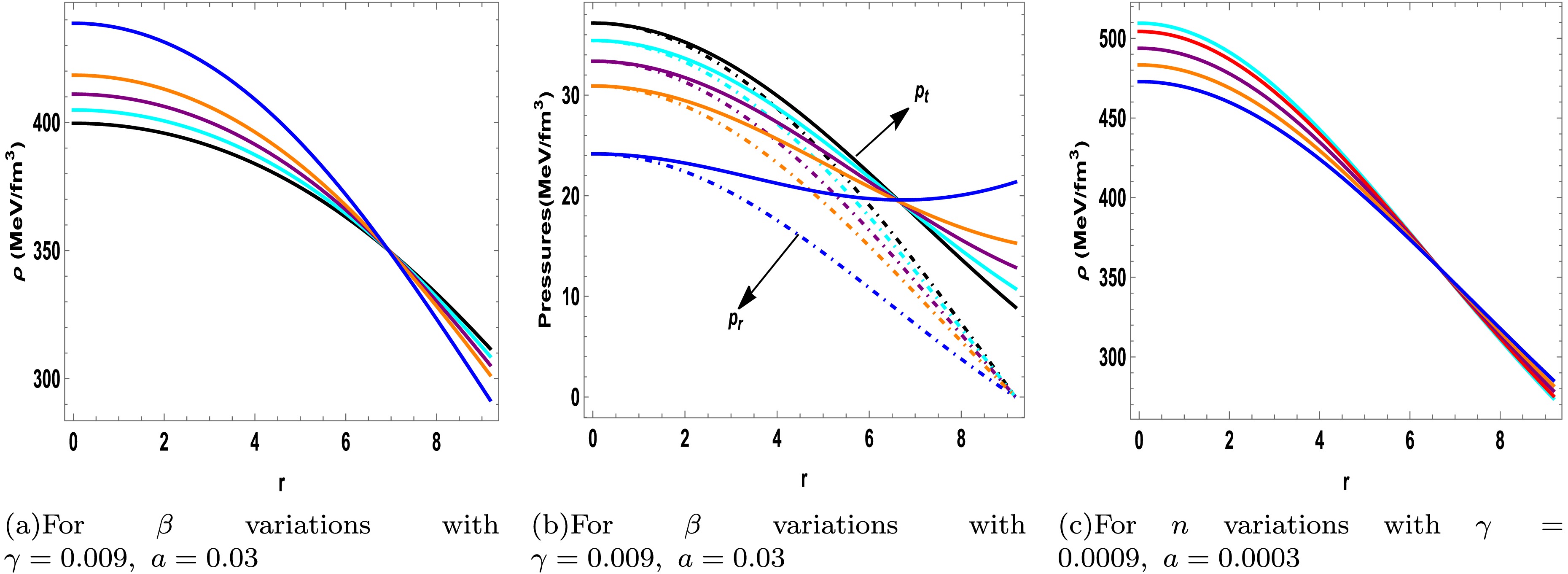
Figure 2. (color online) For the compact star Cen X-3 (
$ {\cal{M}}/{\cal{M}}_{\odot}=1.49 $ ,$ {\cal{R}}=9.178 $ ), the variations in energy density and pressures with the radial coordinate r are shown. Subfigures (a) and (b) depict energy density and pressures ($ p_t \And p_r $ ) for$ n=0.1 $ with$ \beta=0 $ (■),$ \beta=0.5 $ (■),$ \beta=1 $ (■),$ \beta=1.5 $ (■), and$ \beta=2.5 $ (■). Subfigure (c) shows energy density for$ \beta=0.01 $ with$ n=0.5 $ (■),$ n=1 $ (■),$ n=2 $ (■),$ n=3 $ (■), and$ n=4 $ (■). All plots use$ \lambda=1 \times 10^{-12} $ .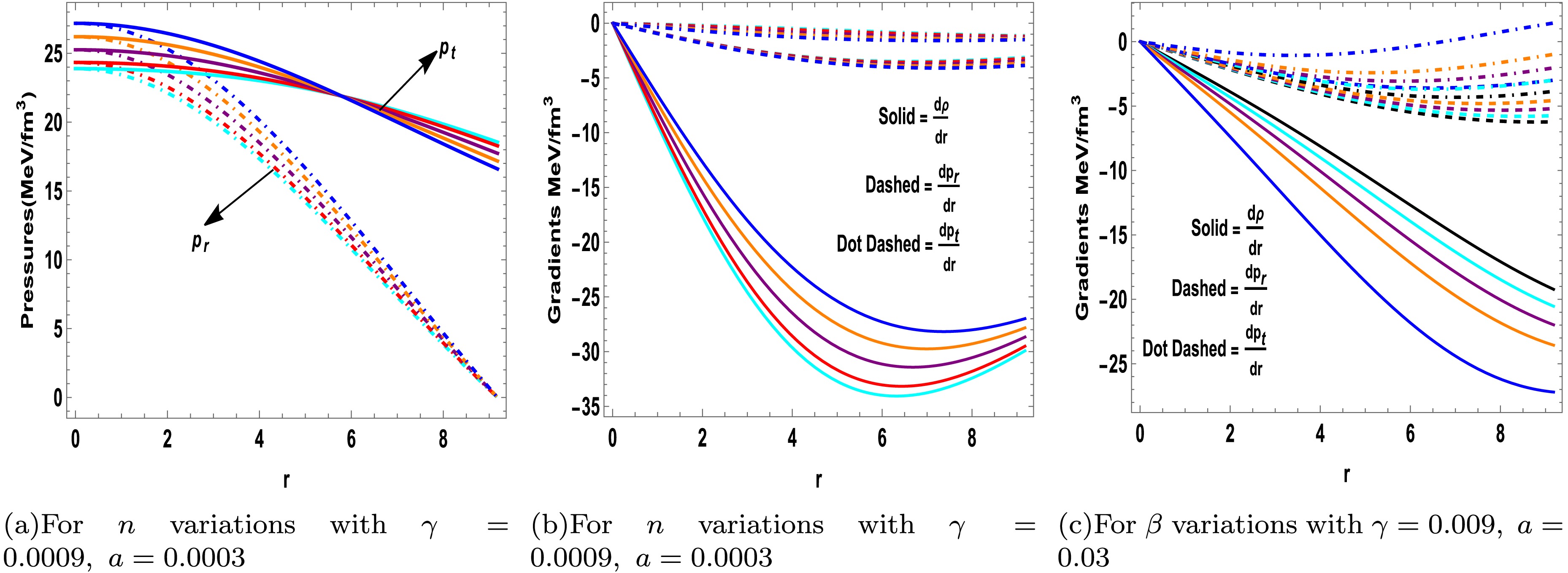
Figure 3. (color online) For the compact star Cen X-3 (
$ {\cal{M}}/{\cal{M}}_{\odot}=1.49 $ ,$ {\cal{R}} = 9.178 $ ), the variations in pressures and gradients with the radial coordinate r are shown. Subfigures (a) and (b) depict pressures ($ p_t \And p_r $ ) and gradients for$ \beta=0.01 $ with$ n=0.5 $ (■),$ n=1 $ (■),$ n=2 $ (■),$ n=3 $ (■), and$ n=4 $ (■), Subfigure (c) shows gradients for$ n=0.1 $ with$ \beta=0 $ (■),$ \beta=0.5 $ (■),$ \beta=1 $ (■),$ \beta=1.5 $ (■), and$ \beta=2.5 $ (■). All plots use$ \lambda=1 \times 10^{-12} $ .$ \begin{aligned} \frac{d \rho}{dr}<0; \quad \frac{dp_r}{dr}<0; \quad \frac{dp_t}{dr}<0 \end{aligned} $

(49) Figures (3(b)) and (3(c)) illustrate the behavior of all gradients under both scenarios. It is observed that the gradients are in accordance with the essential conditions, exhibit a decreasing trend, and vanish at the stellar core, i.e., at
$ r = 0 $ . This behavior is consistent with the physical expectations for a compact star model, where the energy density and pressures reach their maximum at the center and decrease outwards.$ \begin{aligned} \frac{d\rho}{dr}\Bigg|_{r=0}=0; \quad \frac{dp_r}{dr}\Bigg|_{r=0}=0; \quad \frac{dp_t}{dr}\Bigg|_{r=0}=0 \end{aligned} $

(50) -
In self-gravitating bodies—particularly highly dense objects such as compact objects and matter components—the energy density and pressures are anticipated to exhibit characteristic behavior. The energy density and pressures are expected to be maximum at the core of the star, showing finite, positive, and singularies-free behavior, which decreases toward the surface. This behavior supports the stability of the model within the proposed theoretical framework. Figures 2 and 3 illustrate the radial profiles of energy density, as well as the tangential and radial pressures, throughout the radius of the compact star models. The tangential pressure vanishes at the boundary. Furthermore, we analyzed the gradients of the energy density and pressure, which are essential for the construction of a compact star model. It has been posited [75] that these gradients must exhibit negative behavior. We conducted this analysis by considering two specific cases: first, by varying the parameter n while keeping the coupling parameter β constant, and second, by varying β while maintaining a constant value for n. This examination ensures the consistency of our model under the following conditions in both scenarios:
Figure 2. (color online) For the compact star Cen X-3 (
$ {\cal{M}}/{\cal{M}}_{\odot}=1.49 $ ,$ {\cal{R}}=9.178 $ ), the variations in energy density and pressures with the radial coordinate r are shown. Subfigures (a) and (b) depict energy density and pressures ($ p_t \And p_r $ ) for$ n=0.1 $ with$ \beta=0 $ (■),$ \beta=0.5 $ (■),$ \beta=1 $ (■),$ \beta=1.5 $ (■), and$ \beta=2.5 $ (■). Subfigure (c) shows energy density for$ \beta=0.01 $ with$ n=0.5 $ (■),$ n=1 $ (■),$ n=2 $ (■),$ n=3 $ (■), and$ n=4 $ (■). All plots use$ \lambda=1 \times 10^{-12} $ .
Figure 3. (color online) For the compact star Cen X-3 (
$ {\cal{M}}/{\cal{M}}_{\odot}=1.49 $ ,$ {\cal{R}} = 9.178 $ ), the variations in pressures and gradients with the radial coordinate r are shown. Subfigures (a) and (b) depict pressures ($ p_t \And p_r $ ) and gradients for$ \beta=0.01 $ with$ n=0.5 $ (■),$ n=1 $ (■),$ n=2 $ (■),$ n=3 $ (■), and$ n=4 $ (■). Subfigure (c) shows gradients for$ n=0.1 $ with$ \beta=0 $ (■),$ \beta=0.5 $ (■),$ \beta=1 $ (■),$ \beta=1.5 $ (■), and$ \beta=2.5 $ (■). All plots use$ \lambda=1 \times 10^{-12} $ .$ \begin{aligned}\frac{{\rm d}\rho}{{\rm d}r} < 0;\quad\frac{{\rm d}p_r}{{\rm d}r} < 0;\quad\frac{{\rm d}p_t}{{\rm d}r} < 0.\end{aligned} $
(49) Figures 3(b) and 3(c) illustrate the behavior of all gradients in both scenarios. The gradients were in accordance with the essential conditions, exhibited a decreasing trend, and vanished at the stellar core, that is, at
$ r = 0 $ . This behavior is consistent with the physical expectations of a compact star model, where the energy density and pressures reach their maximum at the center and decrease outward.$ \begin{aligned} \frac{{\rm d}\rho}{{\rm d}r}\Bigg|_{r=0}=0; \quad \frac{{\rm d}p_r}{{\rm d}r}\Bigg|_{r=0}=0; \quad \frac{{\rm d}p_t}{{\rm d}r}\Bigg|_{r=0}=0. \end{aligned} $
(50) -
Pressure anisotropy is a crucial factor in assessing the stability of a compact obejct, as it provides valuable insights into the interior stellar structure. For a stable compact star, the anisotropy denoted by Δ, should be non-zero. When the tangential pressure
$ p_t $ exceeds the radial pressure$ p_r $ , the anisotropy Δ is positive ($ \Delta > 0 $ ) and exhibits a repulsive (outward-directed) force. Conversely, if$ p_r $ is greater than$ p_t $ , the anisotropy is negative ($ \Delta < 0 $ ) and refers to an attractive (inward-directed) force [79]. Figures (4(c)) and (5(c)) demonstrate the behavior of anisotropy as a function of radius. It is found that anisotropy is zero at the core and becomes positive, increasing towards the boundary in both cases as shown graphically. This trend confirms the repulsive trend of anisotropy and the necessary anti-gravitational behavior of the anisotropic force for maintaining the stability of stellar structures.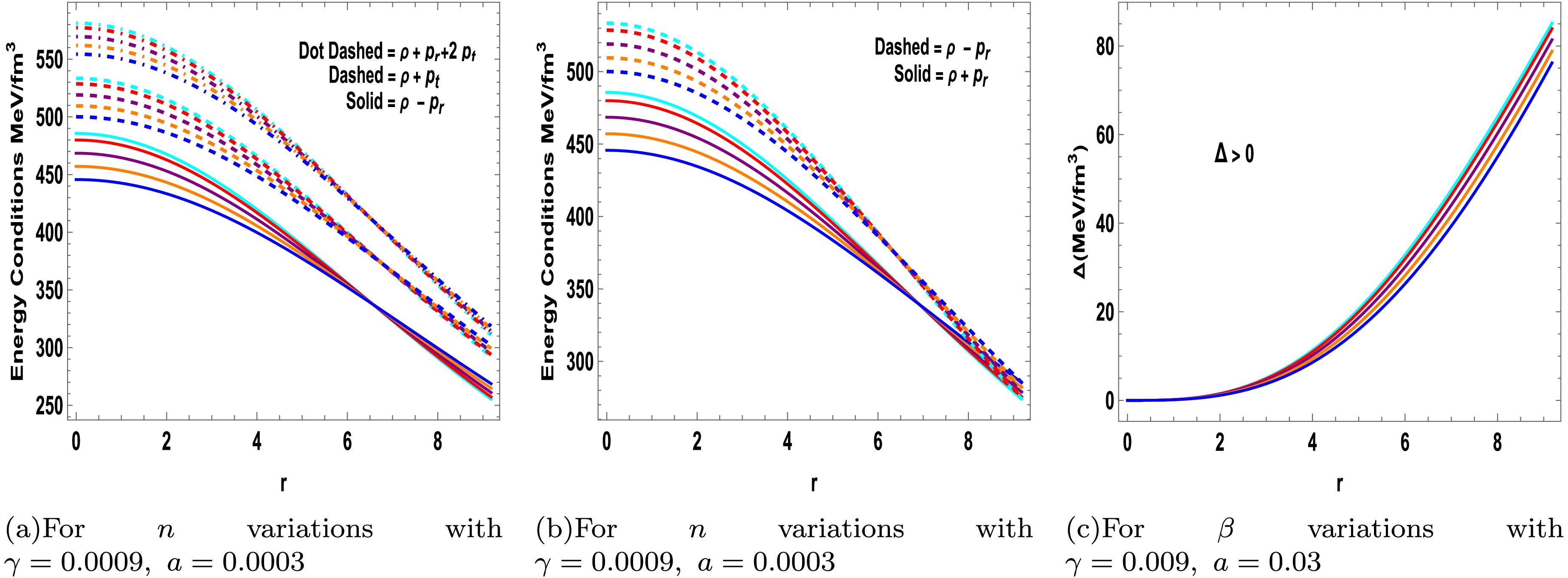
Figure 4. (color online) For the compact star Cen X-3 (
$ {\cal{M}}/{\cal{M}}_{\odot}=1.49 $ ,$ {\cal{R}}=9.178 $ ), the variations in energy conditions and anisotropy with the radial coordinate r are shown. Subfigures (a) and (b) depict energy conditions and (c) depict anisotropy for$ \beta=0.01 $ with$ n=0.5 $ (■),$ n=1 $ (■),$ n=2 $ (■),$ n=3 $ (■), and$ n=4 $ (■). All plots use$ \lambda=1 \times 10^{-12} $ .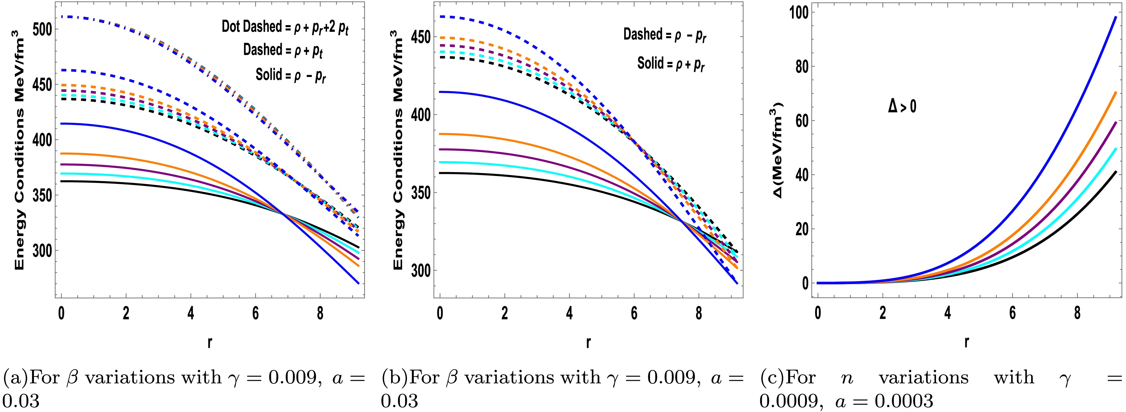
Figure 5. (color online) For the compact star Cen X-3 (
$ {\cal{M}}/{\cal{M}}_{\odot}=1.49 $ ,$ {\cal{R}}=9.178 $ ), the variations in energy conditions and anisotropy with the radial coordinate r are shown. Subfigures (a) and (b) depict energy conditions and (c) depict anisotropy for$ n=0.1 $ with$ \beta=0 $ (■),$ \beta=0.5 $ (■),$ \beta=1 $ (■),$ \beta=1.5 $ (■), and$ \beta=2.5 $ (■). All plots use$ \lambda=1 \times 10^{-12} $ .Energy conditions represent some mathematical constraints on the energy-momentum tensor of self-gravitating bodies and form the root cause of singularity theorems [80] as well as entropy bounds [81]. These conditions are pivotal in assessing the feasibility of a relativistically stable model. The primary energy conditions include the strong energy condition (SEC), weak energy condition (WEC), null energy condition (NEC), and dominant energy condition (DEC). Mathematically, these are provided as below:
$ \begin{aligned} {\bf{NEC}}&: \rho^{eff} \ge 0, \\ {\bf{WEC}}&:\rho^{eff}+p_t^{eff} \ge 0, \quad\quad\quad\quad\quad \rho^{eff}+p_r^{eff}\ge 0.\\ {\bf{SEC}}&:\rho^{eff}+2 p_t^{eff}+p_r^{eff} \ge 0,\\ {\bf{DEC}}&: \rho^{eff}-|p_r^{eff}|\geq 0, \quad\quad\quad\quad\quad \rho^{eff} -|p_t^{eff}|\geq 0. \end{aligned} $

(51) For a physically captivating model, the associated inequalities must be satisfied, ensuring that these energy conditions reach their maximum at the core of the star and remain positive throughout its structure. As showed in Figures (4(a)), (4(b)), (5(a)) and (5(b)), all specified energy conditions are met under both scenarios: when varying the parameter n while keeping the coupling parameter β constant, and when varying β while maintaining n constant. This consistency across both cases further validates the stability of presented models.
Next, we analyze the equilibrium conditions through the involved forces namely the gravitational force (
$ F_g $ ), the hydrostatic force ($ F_h $ ), the anisotropic force ($ F_a $ ) and the modified force ($ F_m $ ) due to our modified$ f({\cal{R}},T,{\cal{L}}_m) $ gravity model. By incorporating the effects of the MGD approach, the extended Tolman-Oppenheimer-Volkoff (TOV) equation for our model is formulated as follows$ \begin{aligned}[b] &-\underbrace{\frac{H(r)^{\prime}}{2}\Bigg[\rho+p_r+\beta(\vartheta^0_0-\vartheta_1^1) \Bigg]\quad}_{ F_g }-\underbrace{\Bigg(\frac{dp_r}{dr}-\beta\frac{d\vartheta^1_1}{dr}\Bigg) \quad}_{ F_h }+\underbrace{\frac{2}{r}\Bigg[p_r-p_r-\beta(\vartheta^0_0-\vartheta_1^1)\Bigg]\quad}_{ F_a }\\ &+\underbrace{\frac{d}{dr}\Bigg[\frac{\gamma}{6(8 \pi G+\gamma+\lambda/2)}\Big((3\rho-p_r-2p_t)+\beta(3\vartheta^0_0+\vartheta_1^1 +2\vartheta^2_2)\Bigg]\Big)}_{ F_m }=0. \end{aligned} $

(52) To ensure the stability of our model within
$ f({\cal{R}},T,{\cal{L}}_m) $ gravity, the total impact of all forces, i.e., gravitational ($ F_g $ ), hydrostatic ($ F_h $ ), anisotropic ($ F_a $ ), and the modified force ($ F_m $ ), must be zero, indicating that these forces are in equilibrium. This balancing effect ensures the stability of any configuration. Figures 6(a) and 6(b) demonstrate the behavior of these forces in two distinct scenarios. In the first scenario, the parameters are held constant while the forces are plotted as functions of varying n as depicted in Figure 6(a). The figure shows that the gravitational force is counteracted by the combined hydrostatic and anisotropic forces, which act in the opposite direction. This equilibrium prevents the gravitational collapse, while the modified force remains constant and exerts only a small impact on the hydrostatic balance. In the second scenario, the forces are plotted for varying values of the coupling parameter β as illustrated in Figure 6(b). This figure confirms that even with different values of β, all forces balance each other, further affirming the stability of our model. These findings validate that our model is not only stable but also represents a physically viable relativistic system.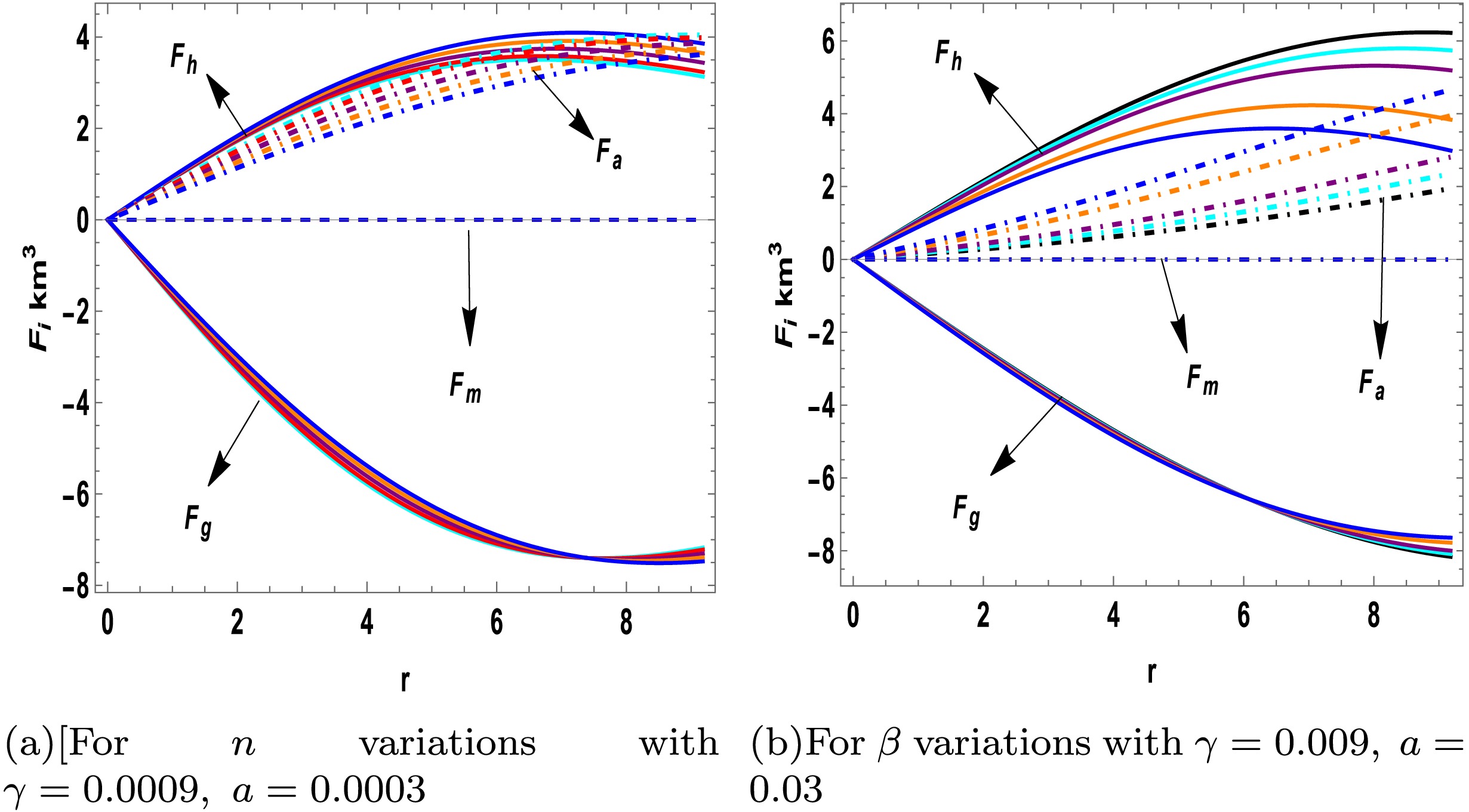
Figure 6. (color online) For the compact star Cen X-3 (
$ {\cal{M}}/{\cal{M}}_{\odot}=1.49 $ ,$ {\cal{R}}=9.178 $ ), the variations in forces with the radial coordinate r are shown. Subfigures (a) depict forces for$ \beta=0.01 $ with$ n=0.5 $ (■),$ n=1 $ (■),$ n=2 $ (■),$ n=3 $ (■), and$ n=4 $ (■), Subfigure (b) shows forces for$ n=0.1 $ with$ \beta=0 $ (■),$ \beta=0.5 $ (■),$ \beta=1 $ (■),$ \beta=1.5 $ (■), and$ \beta=2.5 $ (■). All plots use$ \lambda=1 \times 10^{-12} $ . -
Pressure anisotropy is a crucial factor in assessing the stability of a compact object, because it provides valuable insights into the interior stellar structure. For a stable compact star, the anisotropy—denoted by Δ—should be non-zero. When the tangential pressure
$ p_t $ exceeds the radial pressure$ p_r $ , anisotropy Δ is positive ($ \Delta > 0 $ ) and exhibits a repulsive (outward-directed) force. Conversely, if$ p_r $ is greater than$ p_t $ , anisotropy is negative ($ \Delta < 0 $ ) and refers to an attractive (inward-directed) force [76]. Figures 4(c) and 5(c) demonstrate the behavior of anisotropy as a function of radius. The anisotropy is zero at the core and becomes positive, increasing toward the boundary in both cases, as shown graphically. This trend confirms the repulsive trend of anisotropy and the necessary anti-gravitational behavior of the anisotropic force to maintain the stability of the stellar structures.
Figure 4. (color online) For the compact star Cen X-3 (
$ {\cal{M}}/{\cal{M}}_{\odot}=1.49 $ ,$ {\cal{R}}=9.178 $ ), the variations in energy conditions and anisotropy with the radial coordinate r are shown. Subfigures (a) and (b) depict energy conditions and (c) depicts anisotropy for$ \beta=0.01 $ with$ n=0.5 $ (■),$ n=1 $ (■),$ n=2 $ (■),$ n=3 $ (■), and$ n=4 $ (■). All plots use$ \lambda=1 \times 10^{-12} $ .
Figure 5. (color online) For the compact star Cen X-3 (
$ {\cal{M}}/{\cal{M}}_{\odot}=1.49 $ ,$ {\cal{R}}=9.178 $ ), the variations in energy conditions and anisotropy with the radial coordinate r are shown. Subfigures (a) and (b) depict energy conditions and (c) depicts anisotropy for$ n=0.1 $ with$ \beta=0 $ (■),$ \beta=0.5 $ (■),$ \beta=1 $ (■),$ \beta=1.5 $ (■), and$ \beta=2.5 $ (■). All plots use$ \lambda=1 \times 10^{-12} $ .Energy conditions represent mathematical constraints on the energy-momentum tensor of self-gravitating bodies and form the root cause of singularity theorems [77] and entropy bounds [78]. These conditions are pivotal for assessing the feasibility of relativistically stable models. The primary energy conditions include the strong energy condition (SEC), weak energy condition (WEC), null energy condition (NEC), and dominant energy condition (DEC). Mathematically, these are as follows:
$ \begin{aligned} {\bf{NEC}}&: \rho^{\rm eff} \ge 0, \\ {\bf{WEC}}&:\rho^{\rm eff}+p_t^{\rm eff} \ge 0, \quad\quad\quad\quad\quad \rho^{\rm eff}+p_r^{\rm eff}\ge 0.\\ {\bf{SEC}}&:\rho^{\rm eff}+2 p_t^{\rm eff}+p_r^{\rm eff} \ge 0,\\ {\bf{DEC}}&: \rho^{\rm eff}-|p_r^{\rm eff}|\geq 0, \quad\quad\quad\quad\quad \rho^{\rm eff} -|p_t^{\rm eff}|\geq 0. \end{aligned} $
(51) For a physically captivating model, the associated inequalities must be satisfied to ensure that these energy conditions reach their maximum at the core of the star and remain positive throughout its structure. As shown in Figs. 4(a), 4(b), 5(a), and 5(b), all specified energy conditions are met under both scenarios: when varying the parameter n while keeping the coupling parameter β constant and when varying β while maintaining n constant. This consistency across both cases further validates the stability of the proposed models.
Next, we analyze the equilibrium conditions through the involved forces, that is, the gravitational force (
$ F_g $ ), hydrostatic force ($ F_h $ ), anisotropic force ($ F_a $ ) and modified force ($ F_m $ ) due to our modified$ f({\cal{R}},T,{\cal{L}}_m) $ gravity model. By incorporating the effects of the MGD approach, the extended Tolman-Oppenheimer-Volkoff (TOV) equation for our model is formulated as follows:$ \begin{aligned}[b] &-\underbrace{\frac{H(r)^{\prime}}{2}\Bigg[\rho+p_r+\beta(\vartheta^0_0-\vartheta_1^1) \Bigg]\quad}_{ F_g }-\underbrace{\Bigg(\frac{{\rm d}p_r}{{\rm d}r}-\beta\frac{{\rm d}\vartheta^1_1}{{\rm d}r}\Bigg) \quad}_{ F_h }+\underbrace{\frac{2}{r}\Bigg[p_r-p_r-\beta(\vartheta^0_0-\vartheta_1^1)\Bigg]\quad}_{ F_a }\\ &+\underbrace{\frac{{\rm d}}{{\rm d}r}\Bigg[\frac{\gamma}{6(8 \pi G+\gamma+\lambda/2)}\Big((3\rho-p_r-2p_t)+\beta(3\vartheta^0_0+\vartheta_1^1 +2\vartheta^2_2)\Bigg]\Big)}_{ F_m }=0. \end{aligned} $
(52) To ensure the stability of our model within
$ f({\cal{R}}, T, {\cal{L}}_m) $ gravity, the total impact of all forces, that is, gravitational ($ F_g $ ), hydrostatic ($ F_h $ ), anisotropic ($ F_a $ ), and modified force ($ F_m $ ), must be zero, which implies that these forces are in equilibrium. This balancing effect ensures the stability of all configurations. Figures 6(a) and 6(b) show the behavior of these forces in two distinct scenarios. In the first scenario, the parameters are held constant and the forces are plotted as functions of varying n, as depicted in Fig. 6(a). The figure shows that the gravitational force is counteracted by combined hydrostatic and anisotropic forces, which act in opposite directions. This equilibrium prevents gravitational collapse, whereas the modified force remains constant and exerts only a small impact on the hydrostatic balance. In the second scenario, the forces were plotted for varying values of the coupling parameter β, as illustrated in Fig. 6(b). This figure confirms that even with different values of β, all the forces are balanced, which further confirms the stability of the model. These findings confirm that the model is not only stable but also represents a physically viable relativistic system.
Figure 6. (color online) For the compact star Cen X-3 (
$ {\cal{M}}/{\cal{M}}_{\odot}=1.49 $ ,$ {\cal{R}}=9.178 $ ), the variations in forces with the radial coordinate r are shown. Subfigure (a) depict forces for$ \beta=0.01 $ with$ n=0.5 $ (■),$ n=1 $ (■),$ n=2 $ (■),$ n=3 $ (■), and$ n=4 $ (■). Subfigure (b) shows forces for$ n=0.1 $ with$ \beta=0 $ (■),$ \beta=0.5 $ (■),$ \beta=1 $ (■),$ \beta=1.5 $ (■), and$ \beta=2.5 $ (■). All plots use$ \lambda=1 \times 10^{-12} $ . -
The equation of state represents a dimensionless constraint on the parameters governing radial and tangential pressures. These limitations play a pivotal role in establishing the relationship between the state variables, as expressed by the following equation:
$ \begin{aligned} \omega_t=\frac{p_t}{\rho}, \quad \omega_r=\frac{p_r}{\rho}. \end{aligned} $

(53) It is posited that both parameters must lie between 0 and 1 to ensure the physical stability of a relativistic model and confirm the non-exotic nature of the internal fluid distribution [79]. Figures 7(a) and 7(b) depict the trends of these parameters along the radial direction, with
$ \omega_r $ vanishing at the star boundary for two scenarios—varying n and β—as labeled in the figures. The results clearly demonstrate that both EoS parameters fall within the aforementioned limits, thereby confirming that the solutions are physically viable and consistent with the stable relativistic star models.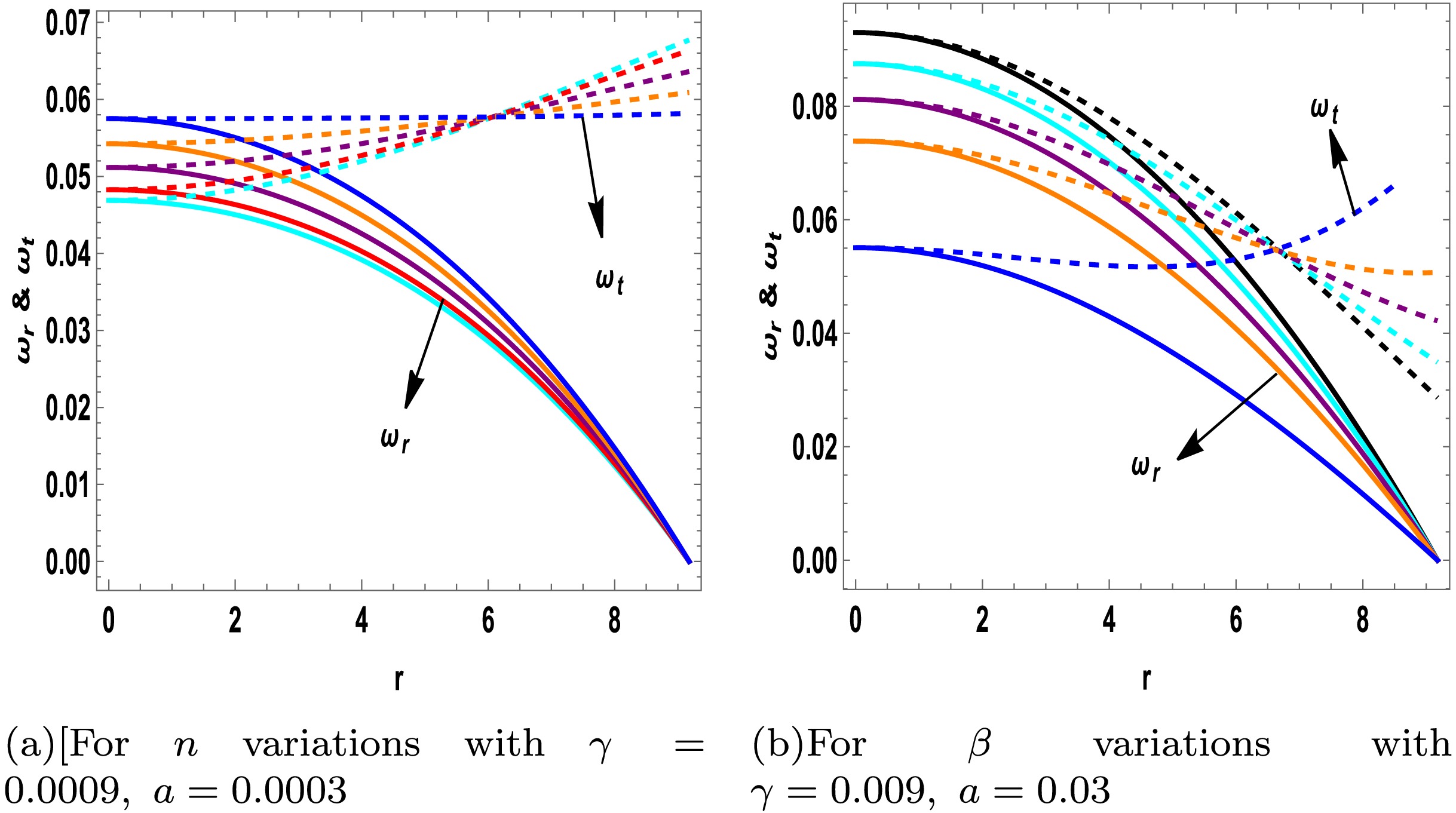
Figure 7. (color online) For the compact star Cen X-3 (
$ {\cal{M}}/{\cal{M}}_{\odot}=1.49 $ ,$ {\cal{R}}=9.178 $ ), the variations in EoS with the radial coordinate r are shown. Subfigure (a) EoS($ w_t \And w_r $ ) for$ \beta=0.01 $ with$ n=0.5 $ (■),$ n=1 $ (■),$ n=2 $ (■),$ n=3 $ (■), and$ n=4 $ (■). Subfigure (b) shows EoS($ w_t \And w_r $ ) for$ n=0.1 $ with$ \beta=0 $ (■),$ \beta=0.5 $ (■),$ \beta=1 $ (■),$ \beta=1.5 $ (■), and$ \beta=2.5 $ (■). All plots use$ \lambda=1 \times 10^{-12} $ .The pressure components must be constrained by the speed of light [80] to evaluate the physical stability of the anisotropic compact star models. This is achieved using Herrera's concept of cracking [81], which defines the expressions for the tangential and radial velocities, as outlined below. Both velocities must lie within the range
$ [0,1] $ , as shown below, which is a requirement termed the causality condition:$ \begin{aligned} v_r^2=\frac{{\rm d}p_r}{{\rm d}\rho}, \quad v_t^2=\frac{{\rm d}p_t}{{\rm d}\rho}. \end{aligned} $

(54) The concept of cracking was further extended by Abreu [82] and Andreasson [83] to assess the stability of stellar structures. This extension is represented by the following equations and inequalities. For a model to be physically promising and potentially stable, it must adhere to the conditions outlined below:
$ \begin{aligned} =\left\{\begin{array}{lr} -1 \leq v_t^2-v_r^2\leq 0, \quad {\rm{Potentially\; stable}};\\ 0<v_t^2-v_r^2\leq 1, \quad\;\;\; {\rm{Potentially\; unstable}}. \end{array} \right. \end{aligned} $

(55) Figures 8(a), 8(b), 8(c), and 9(a) illustrate the radial and tangential velocities (
$ v_r^2 $ and$ v_t^2 $ ) and their differences. As shown, the velocities remain within the specified regions for both scenarios—varying β and n—which confirms the stability of our models. These results reinforce the physical viability and consistency of the model and further validates its capacity to represent a stable relativistic system.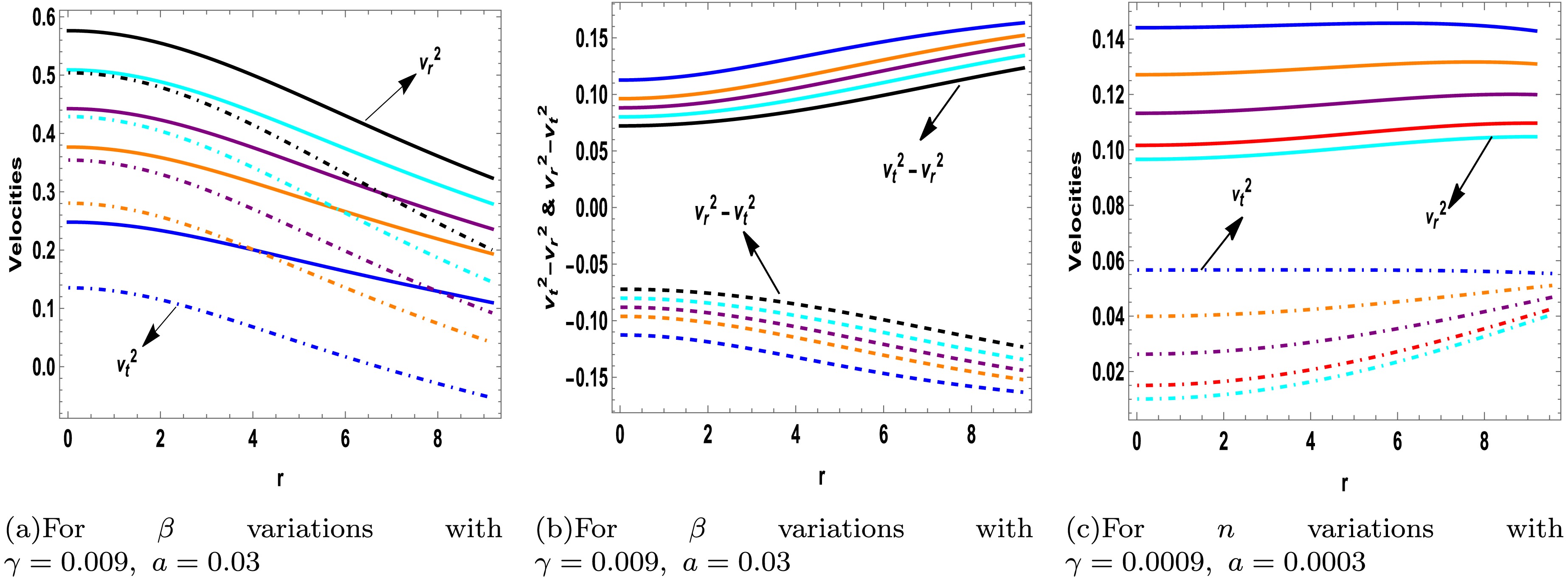
Figure 8. (color online) For the compact star Cen X-3 (
$ {\cal{M}}/{\cal{M}}_{\odot}=1.49 $ ,$ {\cal{R}}=9.178 $ ), the variations in velocities and velocities difference with the radial coordinate r are shown. Subfigures (a) and (b) depict velocities ($ v_t^2 \And v_r^2 $ ) and velocities difference ($ v_t^2-v_r^2 \And v_r^2-v_t^2 $ ) for$ n=0.1 $ with$ \beta=0 $ (■),$ \beta=0.5 $ (■),$ \beta=1 $ (■),$ \beta=1.5 $ (■), and$ \beta=2.5 $ (■). Subfigure (c) shows velocities ($ v_t^2 \And v_r^2 $ ) for$ \beta=0.01 $ with$ n=0.5 $ (■),$ n=1 $ (■),$ n=2 $ (■),$ n=3 $ (■), and$ n=4 $ (■). All plots use$ \lambda=1\times 10^{-12} $ .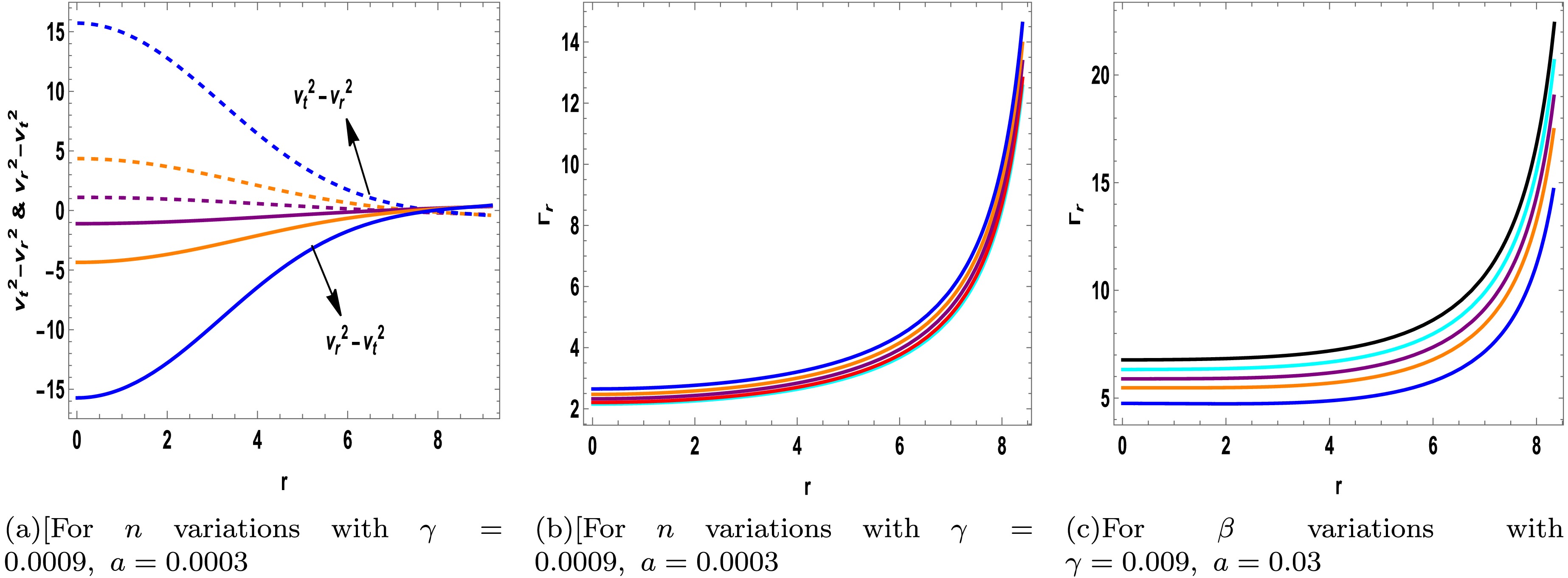
Figure 9. (color online) For the compact star Cen X-3 (
$ {\cal{M}}/{\cal{M}}_{\odot}=1.49 $ ,$ {\cal{R}}=9.178 $ ), the variations in velocities difference and adiabatic index ($ \Gamma_r $ ) with the radial coordinate r are shown. Subfigures (a) and (b) depict the velocities difference ($ v_t^2-v_r^2 \And v_r^2-v_t^2 $ ) and adiabatic index for$ \beta=0.01 $ with$ n=0.5 $ (■),$ n=1 $ (■),$ n=2 $ (■),$ n=3 $ (■), and$ n=4 $ (■). Subfigure (c) shows adiabtic index for$ n=0.1 $ with$ \beta=0 $ (■),$ \beta=0.5 $ (■),$ \beta=1 $ (■),$ \beta=1.5 $ (■), and$ \beta=2.5 $ (■). All plots use$ \lambda=1\times 10^{-12} $ . -
Equation of state represents a dimensionless constraint on the parameters governing the radial and tangential pressures. These limitations play a pivotal role in establishing the relationship between state variables as expressed by the following equation:
$ \begin{aligned} \omega_t=\frac{p_t}{\rho}, \quad \omega_r=\frac{p_r}{\rho}. \end{aligned} $
(53) It is argued that both these parameters must lie between 0 and 1 to ensure the physical stability of a relativistic model and confirm the non-exotic nature of the internal fluid distribution [82]. Figures 7(a) and 7(b) depict the trend of these parameters along the radial direction, with
$ \omega_r $ vanishing at the star's boundary for two scenarios: varying n and varying β, as labeled in the figures. The results clearly demonstrate that both EoS parameters fall within the aforementioned limits, thereby confirming that the solutions are physically viable and consistent referring to stable relativistic star models.
Figure 7. (color online) For the compact star Cen X-3 (
$ {\cal{M}}/{\cal{M}}_{\odot}=1.49 $ ,$ {\cal{R}}=9.178 $ ), the variations in EoS with the radial coordinate r are shown. Subfigures (a) EoS($ w_t \And w_r $ ) for$ \beta=0.01 $ with$ n=0.5 $ (■),$ n=1 $ (■),$ n=2 $ (■),$ n=3 $ (■), and$ n=4 $ (■), Subfigure (b) shows EoS($ w_t \And w_r $ ) for$ n=0.1 $ with$ \beta=0 $ (■),$ \beta=0.5 $ (■),$ \beta=1 $ (■),$ \beta=1.5 $ (■), and$ \beta=2.5 $ (■). All plots use$ \lambda=1 \times 10^{-12} $ .To evaluate the physical stability of anisotropic compact star models, the pressure components must be constrained by the speed of light [83]. This is achieved using Herrera's concept of cracking [84], which defines the expressions for tangential and radial velocities, as outlined below. Both velocities must lie within the range
$ [0,1] $ , a requirement termed as the causality condition.$ \begin{aligned} v_r^2=\frac{dp_r}{d\rho}, \quad v_t^2=\frac{dp_t}{d\rho}. \end{aligned} $
(54) The concept of cracking has been further extended by Abreu [85] and Andreasson [86] to assess the stability of stellar structures. This extension is represented by the following equations and inequalities. For a model to be physically promising and potentially stable, it must adhere the conditions outlined below
$ \begin{aligned} =\left\{\begin{array}{lr} -1 \leq v_t^2-v_r^2\leq 0 \quad {\rm{Potentially\; stable}}\\ 0<v_t^2-v_r^2\leq 1 \quad\;\;\; {\rm{Potentially\; unstable}} \end{array} \right. \end{aligned} $
(55) Figures (8(a)), (8(b)), (8(c)), and (9(a)) illustrate the radial and tangential velocities (
$ v_r^2 $ and$ v_t^2 $ ) and their differences. As shown, the velocities remain within the specified regions for both scenarios: varying β and varying n, which confirm the stability of our models. These results reinforce the physical viability and consistency of the model, further validating its capacity to represent a stable relativistic system.
Figure 8. (color online) For the compact star Cen X-3 (
$ {\cal{M}}/{\cal{M}}_{\odot}=1.49 $ ,$ {\cal{R}}=9.178 $ ), the variations in velocities and velocities difference with the radial coordinate r are shown. Subfigures (a) and (b) depict velocities ($ v_t^2 \And v_r^2 $ ) and velocities difference ($ v_t^2-v_r^2 \And v_r^2-v_t^2 $ ) for$ n=0.1 $ with$ \beta=0 $ (■),$ \beta=0.5 $ (■),$ \beta=1 $ (■),$ \beta=1.5 $ (■), and$ \beta=2.5 $ (■). Subfigure (c) shows velocities ($ v_t^2 \And v_r^2 $ ) for$ \beta=0.01 $ with$ n=0.5 $ (■),$ n=1 $ (■),$ n=2 $ (■),$ n=3 $ (■), and$ n=4 $ (■). All plots use$ \lambda=1\times 10^{-12} $ .
Figure 9. (color online) For the compact star Cen X-3 (
$ {\cal{M}}/{\cal{M}}_{\odot}=1.49 $ ,$ {\cal{R}}=9.178 $ ), the variations in velocities difference and adiabatic index ($ \Gamma_r $ ) with the radial coordinate r are shown. Subfigures (a) and (b) depict the velocities difference ($ v_t^2-v_r^2 \And v_r^2-v_t^2 $ ) and adiabatic index for$ \beta=0.01 $ with$ n=0.5 $ (■),$ n=1 $ (■),$ n=2 $ (■),$ n=3 $ (■), and$ n=4 $ (■), Subfigure (c) shows adiabtic index for$ n=0.1 $ with$ \beta=0 $ (■),$ \beta=0.5 $ (■),$ \beta=1 $ (■),$ \beta=1.5 $ (■), and$ \beta=2.5 $ (■). All plots use$ \lambda=1\times 10^{-12} $ . -
The adiabatic index, which describes the stiffness of the EoS by measuring the change in pressure in response to slight variations in matter density, is a critical factor in analyzing the stability of stellar structures, both relativistically and non-relativistically. Chandrasekhar [84] noted that the adiabatic index should adhere to
$ \Gamma > 4/3 $ , a criterion that has been extensively examined by various authors for both isotropic and anisotropic stellar models [85–86]. The adiabatic indices corresponding to the radial and tangential components are as follows:$ \begin{aligned} \Gamma_r&=\frac{\rho+p_r}{p_r}\Big(\frac{{\rm d}p_r}{{\rm d}\rho}\Big)=\frac{\rho+p_r}{p_r}v_r^2, \end{aligned} $

(56) $ \begin{aligned} \Gamma_t&=\frac{\rho+p_t}{p_t}\Big(\frac{{\rm d}p_t}{{\rm d}\rho}\Big)=\frac{\rho+p_t}{p_t}v_t^2. \end{aligned} $

(57) Figures 9(b) and 9(c) illustrate the conduct of the adiabatic index
$ \Gamma_r $ , demonstrating that its value consistently exceeds 4/3 in both scenarios when varying β and n. This result confirmed the stability of the model under these conditions. The adiabatic index$ \Gamma_t $ was not plotted, as it does not lead to any significant physical insight in this context. Additionally, Moustakidis [87] discussed the critical value of the adiabatic index Γ, emphasizing its strong dependence on the mass-to-radius ratio$ ({\cal{M}}/{\cal{R}}) $ . The critical values of Γ for the seven different stellar candidates are listed in Tables 3 and 4. For all the stellar candidates,$ \Gamma_{{\rm{crit}}} $ exceeds 4/3. The calculation of$ \Gamma_{{\rm{crit}}} $ incorporates the modified mass resulting from gravitational decoupling. These findings further confirmed the stability and physical consistency of our models.Star objects $ M_0/{\cal{M}}_{\odot} $ 

$ {\cal{R}} $ (km)

$ u_0=M_0/{\cal{R}} $ 

$ z_s $ 

$ M/{\cal{M}}_{\odot} $ 

$ u=M/{\cal{R}} $ 

$ z_s $ (MGD)

$ \Gamma_{\rm crit}(MGD) $ 

Her X-1 [69] 0.85 8.1 0.155 0.203153 0.839975 0.152772 0.19999 1.47156 LMC X-4 [70] 1.04 8.301 0.185 0.259026 1.02773 0.182395 0.254704 1.49836 Cen X-3 [71] 1.49 9.178 0.239 0.384532 1.47275 0.236397 0.377241 1.54722 4U 1608-52 [72] 1.74 9.528 0.269 0.471337 1.71993 0.265932 0.461549 1.57394 Vela X-1 1.77 9.56 0.278 0.483339 1.74958 0.269611 0.473173 1.57727 PSR J1614-2230 [73] 1.97 9.69 0.300 0.579186 1.94716 0.296032 0.565684 1.60117 PSR J0740+6620 [74] 2.07 12.34 0.247 0.406152 2.04937 0.244662 0.399352 1.55469 Table 3. Synopsis of total mass along with compactness factor values by utilizing the MGD contribution for parameters (
$ \beta=0.2, $ $ \lambda=1*10^{-12}, a=0.03, \gamma=0.009 $ ).Star objects $ M_0/{\cal{M}}_{\odot} $ 

$ {\cal{R}} $ (km)

$ u_0=M_0/{\cal{R}} $ 

$ z_s $ 

$ M/{\cal{M}}_{\odot} $ 

$ u=M/{\cal{R}} $ 

$ z_s $ (MGD)

$ \Gamma_{\rm crit}(MGD) $ 

Her X-1 [69] 0.85 8.1 0.155 0.203153 0.859676 0.156355 0.206229 1.4748 LMC X-4 [70] 1.04 8.301 0.185 0.259026 1.05183 0.186672 0.263238 1.50223 Cen X-3 [71] 1.49 9.178 0.239 0.384532 1.50664 0.241837 0.391676 1.55214 4U 1608-52 [72] 1.74 9.528 0.269 0.471337 1.75935 0.272028 0.480962 1.57945 Vela X-1 1.77 9.56 0.278 0.483339 1.78969 0.275792 0.493341 1.58286 PSR J1614-2230 [73] 1.97 9.69 0.300 0.579186 1.99201 0.302851 0.59253 1.60734 PSR J0740+6620 [74] 2.07 12.34 0.247 0.406152 2.08997 0.249509 0.412826 1.55908 Table 4. Synopsis of total mass along with compactness parameter values by taking the MGD contribution for parameters (
$ \beta=-0.2, $ $ \lambda=1*10^{-12}, a=0.03, \gamma=0.009 $ ).$ \begin{aligned}\Gamma_{\rm{c}rit}=\frac{4}{3}+\frac{19}{42}\frac{2\cal{M}}{\cal{R}}.\end{aligned} $

(58) -
The adiabatic index, which describes the stiffness of the EoS by measuring the change in pressure in response to slight variations in matter density, is a critical factor in analyzing the stability of stellar structures, both relativistically and non-relativistically. Chandrasekhar noted in his paper [87] that the adiabatic index should adhere to
$ \Gamma > 4/3 $ , a criterion that has been extensively examined by various authors for both isotropic and anisotropic stellar models [88, 89]. The adiabatic index corresponding to the radial and tangential components is provided below$ \begin{aligned} \Gamma_r&=\frac{\rho+p_r}{p_r}\Big(\frac{dp_r}{d\rho}\Big)=\frac{\rho+p_r}{p_r}v_r^2 \end{aligned} $
(56) $ \begin{aligned} \Gamma_t&=\frac{\rho+p_t}{p_t}\Big(\frac{dp_t}{d\rho}\Big)=\frac{\rho+p_t}{p_t}v_t^2. \end{aligned} $
(57) Figures (9(b)) and (9(c)) illustrate the conduct of the adiabatic index
$ \Gamma_r $ , demonstrating that its value consistently exceeds 4/3 in both scenarios when varying β and varying n. This result confirms the stability of the model under these conditions. The adiabatic index$ \Gamma_t $ is not plotted, as this index does not lead to any significant physical insight in this context. Additionally, Moustakidis [90] discusses the critical value of the adiabatic index Γ, emphasizing its strong dependence on the mass-to-radius ratio$ ({\cal{M}}/{\cal{R}}) $ . As shown below, the critical values of Γ for seven different stellar candidates are provided in Tables 3 and 4. In these tables, it can be observed that for all stellar candidates,$ \Gamma_{{\rm{crit}}} $ exceeds 4/3. The calculation of$ \Gamma_{{\rm{crit}}} $ incorporates the modified mass resulting from gravitational decoupling. These findings further affirm the stability and physical consistency of our models.Star objects $ M_0/{\cal{M}}_{\odot} $ $ {\cal{R}} $ (km)$ u_0=M_0/{\cal{R}} $ $ z_s $ $ M/{\cal{M}}_{\odot} $ $ u=M/{\cal{R}} $ $ z_s $ (MGD)$ \Gamma_{crit}(MGD) $ Her X-1 [71] 0.85 8.1 0.155 0.203153 0.839975 0.152772 0.19999 1.47156 LMC X-4 [72] 1.04 8.301 0.185 0.259026 1.02773 0.182395 0.254704 1.49836 Cen X-3 [73] 1.49 9.178 0.239 0.384532 1.47275 0.236397 0.377241 1.54722 4U 1608-52 [74] 1.74 9.528 0.269 0.471337 1.71993 0.265932 0.461549 1.57394 Vela X-1 [75] 1.77 9.56 0.278 0.483339 1.74958 0.269611 0.473173 1.57727 PSR J1614-2230 [76] 1.97 9.69 0.300 0.579186 1.94716 0.296032 0.565684 1.60117 PSR J0740+6620 [77] 2.07 12.34 0.247 0.406152 2.04937 0.244662 0.399352 1.55469 Table 3. Synopsis of total mass along with compactness factor values by utilizing the MGD contribution for parameters (
$ \beta=0.2, \lambda=1*10^{-12}, a=0.03, \gamma=0.009 $ ).Star objects $ M_0/{\cal{M}}_{\odot} $ $ {\cal{R}} $ (km)$ u_0=M_0/{\cal{R}} $ $ z_s $ $ M/{\cal{M}}_{\odot} $ $ u=M/{\cal{R}} $ $ z_s $ (MGD)$ \Gamma_{crit}(MGD) $ Her X-1 [71] 0.85 8.1 0.155 0.203153 0.859676 0.156355 0.206229 1.4748 LMC X-4 [72] 1.04 8.301 0.185 0.259026 1.05183 0.186672 0.263238 1.50223 Cen X-3 [73] 1.49 9.178 0.239 0.384532 1.50664 0.241837 0.391676 1.55214 4U 1608-52 [74] 1.74 9.528 0.269 0.471337 1.75935 0.272028 0.480962 1.57945 Vela X-1 [75] 1.77 9.56 0.278 0.483339 1.78969 0.275792 0.493341 1.58286 PSR J1614-2230 [76] 1.97 9.69 0.300 0.579186 1.99201 0.302851 0.59253 1.60734 PSR J0740+6620 [77] 2.07 12.34 0.247 0.406152 2.08997 0.249509 0.412826 1.55908 Table 4. Synopsis of total mass along with compactness parameter values by taking the MGD contribution for parameters (
$ \beta=-0.2, \lambda=1*10^{-12}, a=0.03, \gamma=0.009 $ ).$ \begin{aligned} \Gamma_{crit}=\frac{4}{3}+\frac{19}{42}\frac{2{\cal{M}}}{{\cal{R}}}. \end{aligned} $
(58) -
In this section, we will talk about the inter-connection between the mass function, compactness, and redshift, as these quantities are inherently related. It is a well-famed result that mass function must exhibit positive increasing behavior and consistent with the radial coordinate limit, i.e.,
$ r \to 0 $ ,$ \mathbb{M}(r) \to 0 $ . The mass reaches its maximum value at the boundary when$ r = {\cal{R}} $ . However, as previously discussed, gravitational decoupling introduces an additional gravitational source, which influences the mass function. Therefore, the modified mass function for the current theory is given by$ \begin{aligned} \mathbb{M}(r)=4 \pi\int_{0}^{r} \rho^{eff}(r_1){r_1}^2 \, dr_1=4 \pi \int_{0}^{r} [\rho(r_1)+\beta \vartheta_0^0(r_1)]{r_1}^2 \, dr_1 \end{aligned} $

(59) or
$ \begin{aligned} \mathbb{M}(r)=\frac{r}{2}\Big(1-e^{-a(r)}\Big)=\frac{r}{2}\Big(1-e^{- W(r)}-\beta \psi(r)\Big). \end{aligned} $

(60) This modification to the mass relation reflects the impact of the supplemental gravitational contributions resulting from the decoupling process, which further affects the structure and dynamics of the compact object. The revised equation can be expressed as follows, with the first component representing the mass at
$ r={\cal{R}} $ derived solely from$ f({\cal{R}},{\cal{L}}_m,T) $ gravity:$ \begin{aligned} M=M_0-\beta \frac{{\cal{R}}}{2}\psi({\cal{R}}), \quad {\rm{where}} \quad M_0=\frac{{\cal{R}}}{2}(1-e^{-W(r)}). \end{aligned} $

(61) This formulation set forth the contributions from standard
$ f({\cal{R}},{\cal{L}}_m,T) $ gravity from those introduced by the gravitational decoupling. The compactness factor [91] for$ f({\cal{R}},{\cal{L}}_m,T) $ gravity due to MGD approach can be written as$ \begin{aligned} u^{eff}=\frac{M}{{\cal{R}}}=u_0-\frac{\beta}{2}\psi({\cal{R}}), \quad {\rm{where}} \quad u_0=\frac{M_0}{{\cal{R}}}. \end{aligned} $

(62) Due to the impact of compactness
$ u^{{\rm{eff}}} $ , the surface gravitational redshift$ z_s $ is also influenced by the decoupling process. Thus, the modified surface redshift$ z_s $ in the context of MGD for$ f({\cal{R}},{\cal{L}}_m,T) $ gravity is expressed [92] as follows:$ \begin{aligned} z_s=\Big(1-2 u_0+\beta \psi({\cal{R}})\Big)^{-1/2}-1, \end{aligned} $

(63) Following the discussion on mass, redshift, and compactness under the gravitational decoupling effect, a few key points can be outlined form the graphical analysis:
● First, it is possible to achieve mass expansion using MGD technique [93] within
$ f({\cal{R}},{\cal{L}}_m,T) $ gravity. As seen from Eq.(61), if the second term is positive, the overall mass increases. In our case, this is possible for negative values of the interaction parameter β. As the mass increases, both the redshift ($ z_s $ ) and compactness (u) also increase. Various authors have previously achieved similar results, as seen in [94], where mass expansion is observed for negative β, while in [95, 96], the authors reported mass expansion for positive coupling parameter values. Tables 3 and 4 displays the values of mass, redshift, and compactness with and without the coupling effect for both negative and positive β values across seven star candidates, respectively. It is noted that mass increases only for positive β values, whereas for negative β, the modified mass is less than the original. Additionally, the critical values of the adiabatic index using Eq.(58) for modified mass using the MGD approach are shown in the table for all stars, and it is observed that the value is greater than 4/3 in both cases (positive and negative β values), confirming the stable trend of the proposed model within the realm of$ f({\cal{R}},{\cal{L}}_m,T) $ gravity. Moreover, Figures (10) and (11) show the plots of modified mass, redshift, and compactness for both cases.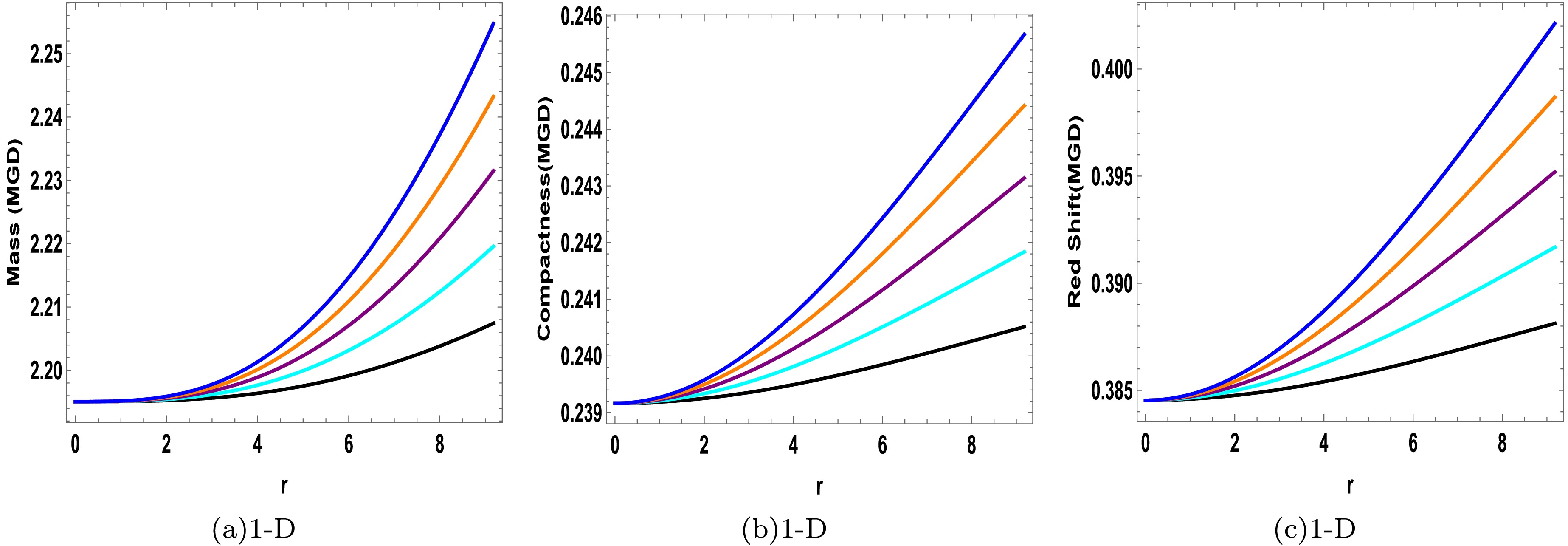
Figure 10. (color online) For the compact star Cen X-3 (
$ {\cal{M}}/{\cal{M}}_{\odot}=1.49 $ ,$ {\cal{R}} =9.178 $ ), the plots show how the mass function, compactness, and redshift vary with the radial coordinate$ r $ . The variation is considered for some variations of$ \beta $ :$ \beta=-0.1 $ (■),$ \beta=-0.2 $ (■),$ \beta=-0.3 $ (■),$ \beta=-0.4 $ (■), and$ \beta=-0.5 $ (■). In all plots, the parameters are set to$ \beta=0.01 $ ,$ a=0.03 $ ,$ \gamma=0.009 $ , and$ \lambda=1\times 10^{-12} $ .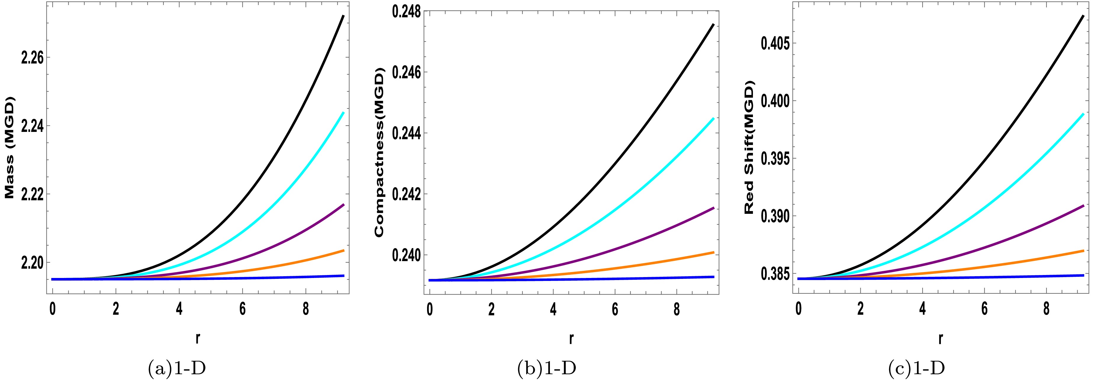
Figure 11. (color online) For the compact star Cen X-3 (
$ {\cal{M}}/{\cal{M}}_{\odot}=1.49 $ ,$ {\cal{R}}=9.178 $ ), the plots show how the mass function, compactness, and redshift vary with the radial coordinate$ r $ . The variation is considered for some values of$ n $ :$ n=0.5 $ (■),$ n=1 $ (■),$ n=1.5 $ (■),$ n=2 $ (■), and$ n=3 $ (■). In all plots, the parameters are set to$ n=0.1 $ ,$ a=0.0003 $ ,$ \gamma=0.0009 $ , and$ \lambda=1\times 10^{-12} $ .● Secondly, the modified compactness due to MGD results in greater compactness compared to the compactness without this effect. Our findings are also consistent with the Buchdahl limits [97] for isotropic fluids (
$ u \leq 4/9 $ ) and anisotropic fluids ($ u\leq 0.30 $ ), which is crucial for establishing a physically acceptable model.Table 5 presents a clear comparative analysis of various anisotropic stellar models developed within different modified gravity frameworks. It highlights the distinct features of each model and illustrates how the present study based on Class-I solutions within the Minimal Geometric Deformation (MGD) approach relates to and extends previous works. By adopting a more generalized gravitational theory, namely
$ f(R,L_m,T) $ , which encompasses earlier special cases, and by utilizing realistic values of mass and radius of compact stars, the model offers a physically consistent anisotropic extension of an initially isotropic seed solution. This comparative framework emphasizes the novelty and physical viability of the present model within the broader context of modified gravity theories.Gravity theory Metric Anstaz Matter Configuration Stability $ \And $ Features

$ f({\cal{R}},T)$ [98]

Krori-Barua metric Anisotropic fluid Physically acceptable; matched with Schwarzschild exterior; consistent graphs for real stars $ f({\cal{T}})$ [99] gravity

Krori-Barua metric Anisotropic fluid Regular and stable; consistent with 4U 1820-30, Her X-1, and SAX J1808.4-3658; surface redshift analyzed $ f({\cal{R}},{\cal{L}}_m,T)={\cal{R}}+\alpha T{\cal{L}}_m $ [100]

Numerical (non-KB) Anisotropic quark matter; MIT bag model Mass–radius relation, adiabatic index, sound speed; α constrained using observational data $ f({\cal{R}}, {\cal{L}}_m, T) $ 

Present WorkClass-1 embedding; MGD approach Anisotropic fluid; radial metric deformation Well-behaved energy density/pressures; negative β yields higher mass; stability via TOV and Herrera cracking condition Table 5. omparison of anisotropic stellar models in various modified gravity frameworks.
It is important to note that mass–radius (M–R) curves provide the most direct diagnostic of stellar configurations. In the present analysis, we have fixed the stellar mass and adopted assumed radii to examine physical behaviour. However, previous works in GR [101],
$ f(R) $ gravity [102−104], and$ f(R,T) $ gravity [105−110], as well as more recent studies in$ f(R,{\cal{L}}_m,T) $ models [111, 112], have shown that matter–geometry couplings significantly shift M–R relations. The compactness and redshift trends we obtain are qualitatively consistent with these results. Our approach differs by employing the generalized$ f(R,{\cal{L}}_m,T) $ framework together with the Minimal Geometric Deformation technique.Unraveling the true mass and radius of pulsars remains one of the central challenges in compact star astrophysics. Despite notable observational progress, these parameters still involve uncertainties due to the extreme physical conditions and complex matter interactions inside such objects. In this work, we propose a refined modeling strategy within the extended
$ f(R,{\cal{L}}_m,T) $ gravity framework to better capture the structure of pulsars under modified gravitational dynamics. To connect our theoretical model with observational reality, we have benchmarked it against reliable data from well-studied pulsars, including Her X-1 [71], LMC X-4 [72], Cen X-3 [73], 4U 1538-52 [74], Vela X-1 [75], PSR J1614-2230 [76], and PSR J0740+6620 [77]. These compact objects span a wide mass range and provide a robust testing ground for assessing the predictive power and flexibility of our model.In future work, we plan to extend this analysis by numerically constructing explicit M–R sequences in
$ f(R,{\cal{L}}_m,T) $ gravity and benchmarking them directly against GR,$ f(R) $ , and$ f(R,T) $ predictions, thereby offering deeper insights into the physics of ultra-dense stars. -
In this section, we discuss the inter-connection between the mass function, compactness, and redshift because these quantities are inherently related. It is well known that the mass function must exhibit a positive increasing behavior and be consistent with the radial coordinate limit, that is,
$ r \to 0 $ ,$ \mathbb{M}(r) \to 0 $ . The mass reaches its maximum value at the boundary when$ r = {\cal{R}} $ . However, as previously discussed, gravitational decoupling introduces an additional gravitational source that affects the mass function. Therefore, the modified mass function for the current theory is given by$ \begin{aligned} \mathbb{M}(r)=4 \pi\int_{0}^{r} \rho^{\rm eff}(r_1){r_1}^2 \, {\rm d}r_1=4 \pi \int_{0}^{r} [\rho(r_1)+\beta \vartheta_0^0(r_1)]{r_1}^2 \, {\rm d}r_1, \end{aligned} $
(59) or
$ \begin{aligned} \mathbb{M}(r)=\frac{r}{2}\Big(1-{\rm e}^{-a(r)}\Big)=\frac{r}{2}\Big(1-{\rm e}^{- W(r)}-\beta \psi(r)\Big). \end{aligned} $
(60) This modification to the mass relation reflects the impact of supplemental gravitational contributions resulting from the decoupling process, which further affects the structure and dynamics of the compact object. The revised equation can be expressed as follows, with the first component representing the mass at
$ r={\cal{R}} $ derived solely from$ f({\cal{R}},{\cal{L}}_m,T) $ gravity, as follows:$ \begin{aligned} M=M_0-\beta \frac{{\cal{R}}}{2}\psi({\cal{R}}), \quad {\rm{where}} \quad M_0=\frac{{\cal{R}}}{2}(1-{\rm e}^{-W(r)}). \end{aligned} $
(61) This formulation sets forth the contributions from the standard
$ f({\cal{R}},{\cal{L}}_m,T) $ gravity from those introduced by gravitational decoupling. The compactness factor [88] for$ f({\cal{R}},{\cal{L}}_m,T) $ gravity owing to the MGD approach can be written as$ \begin{aligned} u^{\rm eff}=\frac{M}{{\cal{R}}}=u_0-\frac{\beta}{2}\psi({\cal{R}}), \quad {\rm{where}} \quad u_0=\frac{M_0}{{\cal{R}}}. \end{aligned} $
(62) Owing to the impact of the compactness
$ u^{{\rm{eff}}} $ , the surface gravitational redshift$ z_s $ is also influenced by the decoupling process. Thus, the modified surface redshift$ z_s $ in the context of the MGD for$ f({\cal{R}},{\cal{L}}_m,T) $ gravity is expressed as follows [89] :$ \begin{aligned} z_s=\Big(1-2 u_0+\beta \psi({\cal{R}})\Big)^{-1/2}-1. \end{aligned} $
(63) Following the discussion of mass, redshift, and compactness under the gravitational decoupling effect, a few key points can be outlined from the graphical analysis.
● First, mass expansion can be achieved using the MGD technique [90] within
$ f({\cal{R}},{\cal{L}}_m,T) $ gravity. As seen from Eq. (61), if the second term is positive, then the overall mass increases. In our case, this is possible for negative values of the interaction parameter β. As the mass increases, both the redshift ($ z_s $ ) and compactness (u) increase. Various authors have previously achieved similar results, as seen in [64], where mass expansion is observed for negative β, whereas in [91–92], the authors reported mass expansion for positive coupling parameter values. Tables 3 and 4 display the values of mass, redshift, and compactness with and without the coupling effect for both negative and positive β values across the seven star candidates. Notably, the mass increases only for positive β values, whereas for negative β, the modified mass is less than the original. Additionally, the critical values of the adiabatic index obtained using Eq. (58) for the modified mass using the MGD approach are shown in the table for all stars. The value is greater than 4/3 in both cases (positive and negative β values), confirming the stable trend of the proposed model within the realm of$ f({\cal{R}},{\cal{L}}_m,T) $ gravity. Moreover, Figs. 10 and 11 show plots of the modified mass, redshift, and compactness for both cases.
Figure 10. (color online) For the compact star Cen X-3 (
$ {\cal{M}}/{\cal{M}}_{\odot}=1.49 $ ,$ {\cal{R}} =9.178 $ ), the plots show how the mass function, compactness, and redshift vary with the radial coordinate$ r $ . The variation is considered for some variations of$ \beta $ :$ \beta=-0.1 $ (■),$ \beta=-0.2 $ (■),$ \beta=-0.3 $ (■),$ \beta=-0.4 $ (■), and$ \beta=-0.5 $ (■). In all plots, the parameters are set to$ \beta=0.01 $ ,$ a=0.03 $ ,$ \gamma=0.009 $ , and$ \lambda=1\times 10^{-12} $ .
Figure 11. (color online) For the compact star Cen X-3 (
$ {\cal{M}}/{\cal{M}}_{\odot}=1.49 $ ,$ {\cal{R}}=9.178 $ ), the plots show how the mass function, compactness, and redshift vary with the radial coordinate$ r $ . The variation is considered for some values of$ n $ :$ n=0.5 $ (■),$ n=1 $ (■),$ n=1.5 $ (■),$ n=2 $ (■), and$ n=3 $ (■). In all plots, the parameters are set to$ n=0.1 $ ,$ a=0.0003 $ ,$ \gamma=0.0009 $ , and$ \lambda=1\times 10^{-12} $ .● Second, the modified compactness due to MGD is greater compared to compactness without this effect. Our findings are also consistent with the Buchdahl limits [93] for isotropic (
$ u \leq 4/9 $ ) and anisotropic fluids ($ u\leq 0.30 $ ), which are crucial for establishing a physically acceptable model.Table 5 presents a clear comparative analysis of the various anisotropic stellar models developed within different modified gravity frameworks. It highlights the distinct features of each model and illustrates how the present study based on Class-I solutions within the MGD approach relates to and extends previous works. By adopting a more generalized gravitational theory, namely
$ f(R,L_m,T) $ , which encompasses earlier special cases, and by utilizing realistic values of mass and radius of compact stars, the model offers a physically consistent anisotropic extension of an initially isotropic seed solution. This comparative framework emphasizes the novelty and physical viability of the present model within the broader context of modified gravity theories.Gravity theory Metric Anstaz Matter Configuration Stability $ \And $ Features$ f({\cal{R}},T)$ [94]Krori-Barua metric Anisotropic fluid Physically acceptable; matched with Schwarzschild exterior; consistent graphs for real stars $ f({\cal{T}})$ [95] gravityKrori-Barua metric Anisotropic fluid Regular and stable; consistent with 4U 1820-30, Her X-1, and SAX J1808.4-3658; surface redshift analyzed $ f({\cal{R}},{\cal{L}}_m,T)={\cal{R}}+\alpha T{\cal{L}}_m $ [96]Numerical (non-KB) Anisotropic quark matter; MIT bag model Mass–radius relation, adiabatic index, sound speed; α constrained using observational data $ f({\cal{R}}, {\cal{L}}_m, T) $
Present WorkClass-1 embedding; MGD approach Anisotropic fluid; radial metric deformation Well-behaved energy density/pressures; negative β yields higher mass; stability via TOV and Herrera cracking condition Table 5. Comparison of anisotropic stellar models in various modified gravity frameworks.
It is important to note that mass–radius (M–R) curves provide the most direct diagnostic of stellar configurations. In the present analysis, we fixed the stellar mass and adopted the assumed radii to examine the physical behavior. However, previous studies on GR [97],
$ f(R) $ gravity [34, 98–99], and$ f(R,T) $ gravity [100−104], as well as more recent studies on$ f(R,{\cal{L}}_m,T) $ models [32, 105], have shown that matter–geometry couplings significantly shift M–R relations. The compactness and redshift trends obtained are qualitatively consistent with these results. Our approach differs by employing the generalized$ f(R,{\cal{L}}_m,T) $ framework together with the MGD technique.Unraveling the true mass and radius of pulsars remains a central challenge in compact star astrophysics. Despite notable observational progress, these parameters still involve uncertainties owing to extreme physical conditions and complex matter interactions inside such objects. In this study, we propose a refined modeling strategy within the extended
$ f(R,{\cal{L}}_m,T) $ gravity framework to better capture the structure of pulsars under modified gravitational dynamics. To connect our theoretical model with observational reality, we compared it to reliable data from well-studied pulsars, including Her X-1 [69], LMC X-4 [70], Cen X-3 [71], 4U 1538-52 [72], Vela X-1 , PSR J1614-2230 [73], and PSR J0740+6620 [74]. These compact objects span a wide mass range and provide a robust testing ground for assessing the predictive power and flexibility of the proposed model.In future work, we plan to extend this analysis by numerically constructing explicit M–R sequences in
$ f(R,{\cal{L}}_m,T) $ gravity and comparing them directly to GR,$ f(R) $ , and$ f(R,T) $ predictions, thereby offering deeper insights into the physics of ultra-dense stars. -
In this research, we employed the MGD approach for gravitational decoupling within the framework of
$ f({\cal{R}}, {\cal{L}}_m, T) $ gravity to construct anisotropic compact star models based on a class-1 embedding spacetime. In the literature, this method has proven to be highly effective for developing interior solutions of self-gravitating systems, enabling the investigation of gravitational effects from various perspectives within spherically symmetric configurations. In the present study, we have utilized Ovalle's gravitational decoupling technique [92] along with the MGD approach in the context of$ f({\cal{R}}, {\cal{L}}_m, T) $ gravity to formulate physically viable models of compact stellar objects with anisotropic pressure. Within this framework, one of the metric potentials is deformed by introducing an additional gravitational source that decouples the original field equations into two separate systems. The first system corresponds to the standard perfect fluid Einstein equations described by$ T_{\mu \nu} $ , whereas the second governs the anisotropic source$ \vartheta_{\mu \nu} $ , forming a quasi-Einstein system. Notably, these two sources interact solely through gravitational interaction, without any direct energy exchange. We introduced deformation by modifying the radial component of the metric through an appropriate choice of the function$ \psi(r) $ [64–65], ensuring regularity in the metric functions and all essential physical parameters throughout the stellar interior. It is important to note that setting the coupling parameter$ \beta = 0 $ recovers the original field equations of the theory. Additionally, constants$ \mathbb{A} $ ,$ \mathbb{B} $ , and c were determined by matching the interior solution to the exterior Schwarzschild geometry.The effective radial pressure,
$ p_r^{{\rm{eff}}} = 0 $ , at the boundary, derived from the second fundamental form of the junction conditions, incorporates both the isotropic pressure$ p_r $ and deformation function$ \psi(r) $ , which arises because of the additional source$ \tilde{\theta}_{\mu\nu} $ . Using realistic observational data, we determined the constants A, B, and c for seven compact stellar candidates: Her X-1, Cen X-3, LMC X-4, Vela X-1, PSR J1614-2230, 4U 1608-52, and PSR J0740+6620. The corresponding results are presented in Tables 1 and 2. The compact star Cen X-3 was selected for graphical examination because its radius ($ {\cal{R}} = 9.178 $ ) lies in an optimal range that allows a comprehensive illustration of all physical parameters, including energy density, pressure profiles, anisotropy, energy conditions, and equilibrium forces. Larger radii were required to exhibit the full behavior of these quantities, making Cen X-3 a suitable candidate. For graphical analysis, we evaluated the physical behavior of the model under two distinct scenarios: one involving variations in the coupling parameter β, and the other involving changes in the deformation parameter n, both using Cen X-3 as the reference model. We summarize the key conclusions derived from this study as follows:● Figures 1(a) and 1(b) show how gravitational decoupling affects the metric potentials for both scenarios when using Cen X-3 star's observational data and constants
$ A = -0.0403881 $ ,$ B = -0.0306402 $ , and$ C = 0.00454612 $ . The metric potentials clearly indicate positive and monotonically decreasing behavior within the star before diminishing at the boundary, fostering our model's regularity and stability.● Figures 2(a), 2(b), 2(c), and 3(a) show positive, non-singular, and monotonically decreasing behaviors of energy density and pressure inside the stellar structure. It was noticed that the radial pressure vanished at the star's surface, validating the model's physical consistency.
● Figures 4(c) and 5(c) depict the trend of the anisotropy profile, which is a positive increasing function of r and is zero at the boundary (indicating that the radial and tangential pressures are equal).
● Figures 3(b) and 3(c) illustrate the negative and monotonically declining gradients of the energy density and pressures, which satisfy the required constraint of vanishing at
$ r=0 $ given in Eq. (50), and hence assured the model's physical validity.● Furthermore, Figs. 4(a), 4(b), 5(a), and 5(b) show the energy condition inequalities, which demonstrate that all energy bounds (NEC, SEC, DEC, and WEC) have been validated throughout the stellar interior given in Eq. (51).
● Figure 6 depicts the hydrostatic equilibrium of the model given by Eq. (52), which is derived from balancing the hydrostatic force (
$ F_h $ ), gravitational force ($ F_g $ ), anisotropic force ($ F_a $ ), and modified force ($ F_m $ ) due to$ f({\cal{R}},{\cal{L}}_m,T) $ gravity. This ensures that the forces counterbalance each other, preventing gravitational collapse and confirming the stability of the model.● The EoS, as shown in Figs. 7(a) and 7(b), indicates that all values are between 0 and 1.
● Additionally, the speeds of sound (
$ v_r^2 \And v_t^2 $ ) remained lower than the speed of light throughout the stellar interface, as shown in Figs. 8 and 9(a). This clearly satisfies the criteria for causality and stability.● Furthermore, the adiabatic index surpasses the essential value of 4/3, thereby guaranteeing static stability. Furthermore, Herrera's cracking conditions were satisfied.
Clearly, the TOV equation holds true in the re-designed framework, indicating that our solutions reflect physically viable, stable, and equilibrium compact star models. Tables 3 and 4 show the mass, redshift, and compactness values, with and without MGD. Notably, we observed that negative values of the coupling parameter β allow for greater mass packing, as evidenced by the increased values of mass, redshift, and compactness compared with that of the un-deformed case. Figure 10 clearly demonstrates that these values increase monotonically with r, reaching the highest value at the surface of the star for
$ \beta=-0.5 $ . Figure 11 shows the effect of varying n with these parameters, with the maximum values occurring at$ n=3 $ for$ \beta=-0.2 $ .This study concludes by highlighting the important effects of gravitational decoupling via the MGD technique on the compactness
$ (u = M/{\cal{R}}) $ and total mass of the compact star models. When β assumes negative values, the additional gravitational source, induced and governed by the coupling parameter β, enables a higher mass confinement within the stellar structure. This realization underscores the flexibility and strength of the MGD approach for constructing stable and physically consistent compact star solutions with anisotropic pressures and extended gravitational influences.In particular, our findings differ from those of previous studies in other modified gravity models, as shown in Table 5, where such significant variation in mass due to deformation and coupling has not been reported within the context of
$ f({\cal{R}}, {\cal{L}}_m, T) $ gravity. Specifically, the simultaneous increase and decrease in mass and compactness with different β values is a novel result of this theory, revealing new physical insights that have not been previously explored. Table 5 presents a comparative summary of our model with other recent studies, clearly emphasizing the theoretical and physical advancements achieved. In$ f(R) $ theory, Sharif and Aslam [106] explored anisotropic spherical symmetric solutions through an extended gravitational decoupling approach. Two types of solutions were presented by considering the Starobinsky model of$ f(R) $ gravity along with the Krori-Barua metric potential. It was shown that one of the two developed models exhibited locally unstable conduct when different coupling parameter values were used. In another study [58], the authors investigated the construction of anisotropic static spheres by using the metric potentials of the Tolman V solution and MGD scheme in$ f(R,T^2) $ gravity. Solutions were obtained by imposing three different constraints, and the first two models were physically viable and stable only when small choices of decoupling parameters were considered. In the present study, we considered the linear$ f(R,L_m,T) $ models and found that for all choices of parameter β, the obtained model exhibited stable and physically valid behavior. In a recent study, Singh et al. [65] explored anisotropic compact star configurations for a self-gravitating structure using a MGD scheme, along with embedding class-1 spacetime in the GR framework. They performed a graphical analysis by considering different variations of the coupling parameters α and n. It is shown that all the physical characteristics are satisfied when positive values of α are considered. Our study extends this work by involving curvature-matter coupling and the results obtained are quite similar. Using the same metric potential with the gravitational coupling approach, Hira et al. [64] modeled compact stellar structures using Rastall theory. Using different measures of graphical analysis, physically valid models were obtained when positive coupling parameter values were assumed, and our results were also in agreement with their findings.The effective implementation of this technique within the framework of
$ f({\cal{R}}, {\cal{L}}_m, T) $ gravity offers promising new directions for the study of compact stars in alternative gravity theories and enhances our understanding of the internal composition and evolution of dense astrophysical objects. -
In this research, we employed the Minimal Geometric Deformation (MGD) approach for gravitational decoupling within the framework of
$ f({\cal{R}}, {\cal{L}}_m, T) $ gravity to construct anisotropic compact star models based on a class-1 embedding spacetime. In the literature, this method has proven highly effective for developing interior solutions of self-gravitating systems, enabling the investigation of gravitational effects from various perspectives within spherically symmetric configurations. In the present work, we utilized Ovalle's gravitational decoupling technique [96] along with the MGD approach in the context of$ f({\cal{R}}, {\cal{L}}_m, T) $ gravity to formulate physically viable models of compact stellar objects with anisotropic pressure. Within this framework, one of the metric potentials was deformed, introducing an additional gravitational source that decoupled the original field equations into two separate systems. The first system corresponds to the standard perfect fluid Einstein equations described by$ T_{\mu \nu} $ , while the second governs the anisotropic source$ \vartheta_{\mu \nu} $ , forming a quasi-Einstein system. Notably, these two sources interact solely through gravitational interaction, without any direct energy exchange. We introduced the deformation by modifying the radial component of the metric through an appropriate choice of the function$ \psi(r) $ [70, 94], ensuring the regularity in the metric functions and all essential physical parameters throughout the stellar interior. It is important to note that setting the coupling parameter$ \beta = 0 $ recovers the original field equations of the theory. Additionally, the constants$ \mathbb{A} $ ,$ \mathbb{B} $ , and c were determined by matching the interior solution to the exterior Schwarzschild geometry.The effective radial pressure
$ p_r^{{\rm{eff}}} = 0 $ at the boundary, derived from the second fundamental form of the junction conditions, incorporates both the isotropic pressure$ p_r $ and the deformation function$ \psi(r) $ , which arises due to the additional source$ \tilde{\theta}_{\mu\nu} $ . Using realistic observational data, we have determined the constants A, B, and c for seven compact stellar candidates: Her X-1, Cen X-3, LMC X-4, Vela X-1, PSR J1614-2230, 4U 1608-52, and PSR J0740+6620, with the corresponding results presented in Tables 1 and 2. The compact star Cen X-3 has been chosen for graphical examination because its radius ($ {\cal{R}} = 9.178 $ ) lies in an optimal range that allows comprehensive illustration of all physical parameters, including energy density, pressure profiles, anisotropy, energy conditions, and equilibrium forces. Larger radii were required to exhibit the full behavior of these quantities, making Cen X-3 a suitable candidate. For graphical analysis, we evaluated the physical behavior of the model under two distinct scenarios: one involving variations in the coupling parameter β, and the other involving changes in the deformation parameter n, both using Cen X-3 as the reference model. In the following, we summarize the key conclusions derived from this study:● Figures (1(a)) and (1(b)) showed how gravitational decoupling affects the metric potentials for both scenarios, using Cen X-3 star's observational data and constants
$ A = -0.0403881 $ ,$ B = -0.0306402 $ , and$ C = 0.00454612 $ . The metric potentials have clearly indicated positive and monotonically decreasing behavior within the star before diminishing at the boundary, fostering our model's regularity and stability.● Figures (2(a)), (2(b)), (2(c)), and (3(a)) have shown positive, non-singular, and monotonically decreasing behavior of energy density and pressures inside the stellar structure. It has been noticed that radial pressure vanishes at the star's surface, validating the model's physical consistency.
● Figures (4(c)) and (5(c)) depicted the trend of anisotropy profile, which is positive increasing function of r and turns out to be zero at the boundary (indicating that the radial and tangential pressures are equal there).
● Figures (3(b)) and (3(c)) have illustrated negative and monotonically declining gradients of energy density and pressures, which satisfied the required constraint of vanishing at
$ r=0 $ given in Eq.(50), and hence assured the model's physical validity.● Furthermore, Figures (4(a)), (4(b)), (5(a)), and (5(b)) have shown the energy condition inequalities, which demonstrated that all energy bounds (NEC, SEC, DEC, and WEC) have been validated throughout the stellar interior given in Eq.(51).
● Figure (6) has depicted the model's hydrostatic equilibrium given by Eq.(52), which is derived from the balancing of hydrostatic force (
$ F_h $ ), gravitational force ($ F_g $ ), anisotropic force ($ F_a $ ), and the modified force ($ F_m $ ) due to$ f({\cal{R}},{\cal{L}}_m,T) $ gravity. This ensures that the forces counter balance one another, preventing the gravitational collapse and confirming the model's stability.● The EoS, as shown in the Figures (7(a)) and (7(b)), indicated that all values are between 0 and 1.
● Also, the speed of sounds (
$ v_r^2 \And v_t^2 $ ) remained lower than the speed of light throughout the stellar interior as shown in Figures (8) and (9(a)). This clearly meets the criteria for causality and stability.● Furthermore, the adiabatic index surpasses the essential value of 4/3, guaranteeing the static stability. Furthermore, Herrera's cracking condition has been met.
Clearly, the TOV equation has held true in the re-designed framework, indicating that our solutions reflect physically viable, stable, and equilibrium compact star models. Tables (III) and (IV) show the mass, redshift, and compactness values, with and without minimal geometric deformation. Notably, we have observed that negative values of the coupling parameter β allow for greater mass packing, as evidenced by the increased values of mass, redshift, and compactness compared to the un-deformed case. Figure (10) clearly demonstrated that these values rise monotonically with r, reaching a highest value at the star's surface for
$ \beta=-0.5 $ . Figure (11) showed how varying n affects these parameters, with the maximum values occurring at$ n=3 $ for$ \beta=-0.2 $ .This work concludes by highlighting the important effects of gravitational decoupling via the MGD technique on the compactness
$ (u = M/{\cal{R}}) $ and total mass of compact star models. When β takes negative values, the additional gravitational source induced and governed by the coupling parameter β enables higher mass confinement within the stellar structure. This realization underscores the flexibility and strength of the MGD approach in constructing stable and physically consistent compact star solutions with anisotropic pressures and extended gravitational influences.In particular, our findings differ from previous studies in other modified gravity models, as shown in the comparative Table 5, where such significant variation in mass due to deformation and coupling has not been reported within the context of
$ f({\cal{R}}, {\cal{L}}_m, T) $ gravity. Specifically, the simultaneous increase and decrease in mass and compactness with different β values is a novel result in this theory, revealing new physical insights that have not been previously explored. Table 5 presents a comparative summary of our model with other recent works, clearly emphasizing the theoretical and physical advancements achieved. In$ f(R) $ theory, Sharif and Aslam [113] explored anisotropic spherical symmetric solutions through extended gravitational decoupling approach. By considering Starobinsky model of$ f(R) $ gravity along with Krori-Barua metric potential, two sorts of solutions have been presented. It has been shown that one of the two developed models exhibited locally unstable conduct when different values of coupling parameter are used. In another study [58], authors investigated the construction of anisotropic static spheres by using the metric potentials of Tolman V solution and minimal geometric deformation scheme in$ f(R,T^2) $ gravity. Solutions were obtained by imposing three different constraints, it has been found that first two models are physically viable and stable only when small choices of decoupling parameter are taken. In present work, we have considered linear$ f(R,L_m,T) $ model and it has been found that for all choices of β parameter, the obtained model exhibited stable and physically valid behavior. In a recent work, Singh et al. [65] have explored anisotropic compact star configurations for self-gravitating structure through minimal geometric deformation scheme along with of embedding class-1 spacetime in GR framework. They performed the graphical analysis by considering different variations of coupling parameter α and n. It is shown that all physical characteristics are satisfied when positive values of α are considered. Our work is an extension of this work by involving curvature-matter coupling and the results obtained are quite similar. Using same metric potential along with gravitational coupling approach, Hira et al. [64] modeled some compact stellar structures in Rastall theory. Through graphical analysis of different measures, physically valid models are obtained when positive coupling parameter values are taken, and our obtained results are also in agreement with their findings.The effective implementation of this technique within the framework of
$ f({\cal{R}}, {\cal{L}}_m, T) $ gravity offers promising new directions for the study of compact stars in alternative gravity theories and enhances our understanding of the internal composition and evolution of dense astrophysical objects.
Stellar configurations in f(R, Lm, T) gravity: probing anisotropy and stability via minimal geometric deformation
- Received Date: 2025-06-30
- Available Online: 2026-02-15
Abstract: This study uses a minimal geometric deformation scheme within the


 DownLoad: