


 Abstract
 HTML
HTML Reference
 Related
 PDF
PDF


-
As extremely dense celestial bodies predicted by General Relativity (GR), black holes have captivated the scientific community with their extreme gravitational effects and event horizon dynamics. The landmark detection of binary black hole mergers by the Laser Interferometer Gravitational-Wave Observatory (LIGO) [1−3] established the first direct evidence for astrophysical black holes, while the Event Horizon Telescope (EHT) collaboration's 1.3 mm interferometric imaging of M87's central supermassive black hole [4−9] marked the dawn of visual black hole astronomy. Subsequent EHT observations of Sagittarius A* (Sgr A*) [10−15] demonstrated that the photon ring angular diameter agrees with GR's predicted shadow size within 10% uncertainty. These millimeter-wave interferometric measurements essentially map the black hole shadow's angular scale, providing empirical constraints on black hole mass, spin, and strong-field spacetime geometry. Given the shadow morphology's acute sensitivity to spacetime curvature, it has become a powerful diagnostic tool for testing gravitational theories and quantifying black hole parameters [16−32].
Although the black hole itself does not emit light, its strong gravity attracts the surrounding hot, magnetized plasma, forming a luminous accretion disk around the black hole. These disks—composed of relativistic gas and dust orbiting near the speed of light—emit multiwavelength radiation spanning X-ray to infrared regimes [33]. During accretion episodes, a fraction of infalling material escapes along the black hole's rotation axis, generating collimated relativistic jets. Both the accretion flow and jets act as primary illumination sources for horizon-scale imaging, with their radiation patterns critically shaping the observed shadow morphology. The foundational work by Luminet [34] employed semi-analytical methods to simulate Schwarzschild black hole shadows, revealing that the shadow's apparent size depends on both the accretion flow's outer boundary and the central brightness depression. Subsequent studies extended this framework to Kerr black holes with Keplerian accretion disks [35], while general relativistic ray-tracing techniques enabled investigations of thick accretion disks [36]. Recent advances systematically explore the optical observation appearance of black holes in diverse accretion scenarios: spherical accretion models [37−40], optically/geometrically thin disks [41−58] and geometrically thick accretion disk models [59, 60]. By conducting in-depth analyses of these models, a more comprehensive understanding of the distinct characteristics of black hole shadows across various spacetime backgrounds can be attained.
With the ongoing development of observational technological infrastructure, researchers are now able to utilize experimental techniques with improved precision and resolution to systematically validate the theoretical predictions of General Relativity (GR) across a wide range of astrophysical environments, from weak gravitational fields to strong-field regimes [61, 62]. These groundbreaking developments not only consolidate the theoretical foundation of GR from multiple dimensions but also drive systematic revisions of the theory. Among prevailing modification schemes, the reconstruction of GR's theoretical framework through Einstein action modifications represents a pivotal approach, where the introduction of Kalb-Ramond (KR) geometric structures emerges as a critical methodological breakthrough for such theoretical extensions [63]. As a two-form quantum field, the KR field is hypothesized to be associated with closed string excitations within the framework of heterotic string theory [64]. Studies have demonstrated that the nonminimal coupling between the gravitational sector and the non-zero vacuum expectation value of the tensor field leads to spontaneous Lorentz symmetry violation [65]. Recently, Khodadi studied rapidly rotating black holes in the presence of Lorentz symmetry violation parameters, which differ from Kerr black holes, and explored the energy extraction phenomenon induced by magnetic reconnection in the ergosphere [66]. Additionally, they investigated slowly rotating black holes modified by Lorentz symmetry violation and analyzed the energy deposition rate of neutrinos producing gamma-rays from annihilation in the equatorial plane of the black hole [67]. Research in the KR field has led to several significant conclusions, including the derivation of the antisymmetric tensor of a second-rank, which is interpreted as the source of spacetime torsion, the intrinsic angular momentum of objects, and the diverse structures of distant galaxies attributed to topological defects [68, 69]. Further studies on KR field gravity and its effects on particles can be found in the references [70−72].
As an effective platform for testing gravitational theory, the investigation of black hole shadows within the framework of KR gravity has naturally garnered considerable attention. Kumar et al. investigated the shadow profile and strong gravitational lensed effect of rotating black holes in KR gravity [73]. while Zubair et al. constrained Lorentz-violation parameters through shadow-radius comparisons with EHT observations [74]. Complementary work by Liu et al. modeled shadows of slowly rotating KR black holes under isotropic emission [75]. However, these studies mainly focus on slowly rotating black holes or neglect accretion disk models, while the accretion disk plays a crucial role in black hole shadow imaging. Therefore, this paper will explore the shadow images of black holes with general rotation parameters in KR gravity under the spherical light source and thin accretion disk models. We will focus on the influence of relevant physical parameters, observation inclination and the state of accretion material on the shadow image.
The structure of this paper is arranged as follows. In Section 2, we briefly discuss the action of the KR field, static and rotating black holes in KR gravity, and derive the photon geodesic equation. Based on this, we generate the shadow images of rotating black holes by introducing celestial coordinates. In Section 3, we present the black hole shadow image under spherical light sources using the backward ray-tracing techniques. In Section 4, we consider an optically and geometrically thin accretion disk located at the equatorial plane as a light source and plot the black hole shadow image. We will focus on the influence of black hole parameters and observation inclination on the shadow image. In Section 5, we analyze in detail the redshift factor distribution of direct and lensed images. Finally, we summarize the main conclusions and provide further discussions.
-
Black holes are extremely dense celestial bodies predicted by General Relativity (GR), and have captivated the scientific community with their significant gravitational effects and event horizon dynamics. The landmark detection of binary black hole mergers by the Laser Interferometer Gravitational-Wave Observatory (LIGO) [1−3] established the first direct evidence for astrophysical black holes, while the Event Horizon Telescope (EHT) collaboration's 1.3 mm interferometric imaging of M87's central supermassive black hole [4−9] marked the dawn of visual black hole astronomy. Subsequent EHT observations of Sagittarius A* (Sgr A*) [10−15] demonstrated that the photon ring angular diameter agrees with GR's predicted shadow size within 10% uncertainty. These millimeter-wave interferometric measurements map the black hole shadow's angular scale, providing empirical constraints on the mass, spin, and strong-field spacetime geometry of black holes. Given the shadow morphology's acute sensitivity to spacetime curvature, it is considered a powerful diagnostic tool for testing gravitational theories and quantifying black hole parameters [16−32].
Although the black hole itself does not emit light, its strong gravity attracts hot, magnetized plasma from its surrounding to form a luminous accretion disk around it. These disks—comprising relativistic gas and dust orbiting near the speed of light—emit multiwavelength radiation spanning X-ray to infrared regimes [33]. During accretion episodes, a fraction of infalling material escapes along the black hole's rotation axis, generating collimated relativistic jets. Both the accretion flow and jets act as primary illumination sources for horizon-scale imaging, with their radiation patterns critically shaping the observed shadow morphology. The foundational work by Luminet [34] employed semi-analytical methods to simulate Schwarzschild black hole shadows, revealing that the shadow's apparent size depends on both the accretion flow's outer boundary and the central brightness depression. Subsequent studies extended this framework to Kerr black holes with Keplerian accretion disks [35], while general relativistic ray-tracing techniques enabled investigations of thick accretion disks [36]. Recent advances systematically explore the optical observation appearance of black holes in diverse accretion scenarios: spherical accretion models [37−40], optically/geometrically thin disks [41−58], and geometrically thick accretion disk models [59, 60]. By conducting in-depth analyses of these models, a more comprehensive understanding of the distinct characteristics of black hole shadows across various spacetime backgrounds can be attained.
With the ongoing development of observational technological infrastructure, researchers can now utilize experimental techniques with improved precision and resolution to systematically validate the theoretical predictions of GR across a wide range of astrophysical environments, from weak gravitational fields to strong-field regimes [61, 62]. These groundbreaking developments not only consolidate the theoretical foundation of GR from multiple dimensions but also drive systematic revisions of the theory. Among prevailing modification schemes, the reconstruction of GR's theoretical framework through Einstein action modifications represents a pivotal approach, where the introduction of Kalb-Ramond (KR) geometric structures emerges as a critical methodological breakthrough for such theoretical extensions [63]. As a two-form quantum field, the KR field is hypothesized to be associated with closed string excitations within the framework of heterotic string theory [64]. Studies show that the nonminimal coupling between the gravitational sector and the non-zero vacuum expectation value of the tensor field leads to spontaneous Lorentz symmetry violation [65]. Recently, Khodadi studied rapidly rotating black holes in the presence of Lorentz symmetry violation parameters, which differ from Kerr black holes, and explored the energy extraction phenomenon induced by magnetic reconnection in the ergosphere [66]. Additionally, they investigated slowly rotating black holes modified by Lorentz symmetry violation and analyzed the energy deposition rate of neutrinos producing gamma-rays from annihilation in the equatorial plane of the black hole [67]. Research in the KR field has led to several significant conclusions, including the derivation of the antisymmetric tensor of a second-rank, which is interpreted as the source of spacetime torsion, the intrinsic angular momentum of objects, and the diverse structures of distant galaxies attributed to topological defects [68, 69]. Further studies on KR field gravity and its effects on particles can be found in the references [70−72].
As an effective platform for testing gravitational theory, the investigation of black hole shadows within the framework of KR gravity has naturally garnered considerable attention. Kumar et al. investigated the shadow profile and strong gravitational lensed effect of rotating black holes in KR gravity [73], while Zubair et al. constrained Lorentz-violation parameters through shadow-radius comparisons with EHT observations [74]. Complementary work by Liu et al. modeled shadows of slowly rotating KR black holes under isotropic emission [75]. However, these studies mainly focus on slowly rotating black holes or neglect accretion disk models, while the accretion disk plays a crucial role in black hole shadow imaging. Therefore, this study explores the shadow images of black holes with general rotation parameters in KR gravity under the spherical light source and thin accretion disk models. We focus on the influence of relevant physical parameters, observation inclination and the state of accretion material on the shadow image.
The remainder of this paper is structured as follows. In Section II, we briefly discuss the action of the KR field, static and rotating black holes in KR gravity, and derive the photon geodesic equation. Accordingly, we celestial coordinates to generate the shadow images of rotating black holes. In Section III, we present the black hole shadow image under spherical light sources using the backward ray-tracing techniques. In Section IV, we consider an optically and geometrically thin accretion disk located at the equatorial plane as a light source and plot the black hole shadow image. Here, we focus on the influence of black hole parameters and observation inclination on the shadow image. In Section V, we analyze in detail the redshift factor distribution of direct and lensed images. Finally, we summarize the main conclusions and provide further discussions.
-
Consider the nonminimal coupling between the gravity and a self-interacting KR field [76]
$ \begin{aligned}[b] S =\;& \int \sqrt{-g} \, {\rm d}^4x \Bigg[ \frac{R}{16\pi} - \frac{1}{12} H_{abc}H^{abc} - V\left(T_{ab}T^{ab} \pm t_{ab}t^{ab}\right) \\ &+ \frac{1}{16\pi} \left( \xi_1 T^{ab} T_b^c R_{ac} + \xi_2 T_{ab}T^{ab}R \right) \Bigg], \end{aligned} $
(1) where g is the determinant of the metric tensor
$ g_{ab} $ ,$ R = g^{ab}R_{ab} $ is the scalar curvature, and$ R_{ab} $ is the Ricci tensor. The KR field is defined by the antisymmetric tensor field$ T_{ab} $ , satisfying$ T_{ab} = -T_{ba} $ , and the potential V depends on the expectation value of the tensor field$ T_{ab} $ . The parameters$ \xi_1 $ and$ \xi_2 $ are the nonminimal coupling constants. For convenience, we adopt geometric units ($ G = c = 1 $ ). The existence of the KR field leads to the violation of Lorentz symmetry, i.e., wherein the vacuum expectation value is$ \langle T_{ab} \rangle = t_{ab} \neq 0 $ [63], and the tensor field$ T_{ab} $ can be decomposed into a timelike vector and two spacelike vectors, similar to the decomposition of the electromagnetic field tensor$ F_{ab} $ [65]. The tensor$ H_{abc} = \partial_a T_{bc} $ is also an antisymmetric tensor, satisfying$ H_{abc} = H_{[abc]} $ . Formally,$ H_{abc} $ is similar to$ F_{ab} $ , while$ T_{ab} $ is analogous to the electromagnetic four-potential$ A_a $ .In [76], the authors postulate that the KR field exists in a vacuum environment, thereby fulfilling the condition
$ T^{ab}T_{ab} = t^{ab}t_{ab} $ . In flat spacetime, the vacuum expectation value of Lorentz symmetry violation, denoted as$ t_{ab} $ , is treated as a constant field, satisfying$ \partial_a t_{bc} = 0 $ . Additionally, it possesses a constant norm given by$ t^2 = t^{ab}t_{ab} $ . Under these conditions, the strength of the KR field diminishes, thereby demonstrating$ t_{ab} $ as a constant tensor with a vanishing Hamiltonian. By invoking the minimal substitution principle, the assumption is generalized to curved spacetime. In this context, the vacuum expectation value of the KR field is also considered constant, thereby satisfying the condition$ \nabla_a t_{bc} = 0 $ . This ensures that both the KR field strength and the associated Hamiltonian remain identically zero. Based on this theoretical framework, one can derive the solution for static black holes in KR gravity, assuming that the KR vacuum expectation value$ t_{ab} $ has a constant norm and the corresponding Hamiltonian is zero. The modified Einstein field equation is given by$ R_{ab}-\frac{1}{2}Rg_{ab} = 8 \pi {\cal{T}}_{ab}^{{\xi_{1}}}, $
(2) where
$ {\cal{T}}_{ab}^{{\xi_{1}}} $ is the energy-momentum tensor. The general form of the static spherically symmetric metric is$ {\rm d}s^2 = -A(r){\rm d}t^2+B(r)^{-1}{\rm d}r^2+r^2\left({\rm d}\theta^2+\sin^2\theta \, {\rm d}\phi^2\right). $
(3) The KR vacuum expectation value can be written as
$ t_{ab} = -E(r) \left[ ({\rm d}t)_a \wedge ({\rm d}r)_b \right], $
(4) where
$ t_{01} = -E $ . As mentioned earlier, the norm of the KR field$ t^2 = t^{ab} t_{ab} $ is constant. For the metric (3),$ E(r) $ satisfies$ E(r) = |t|\sqrt{\frac{A(r)}{2B(r)}}, $
(5) where t is a constant. This describes a static pseudo-electric field in the radial direction, i.e.,
$ E^a = (0, E, 0, 0) $ . Substituting the metric (3) into the modified Einstein field Eq. (2), we obtain$ A(r) = B(r) = 1 - \frac{2M}{r} +\frac{{\cal{G}}}{r^{\frac{2}{\lambda}}}. $
(6) Therefore, the static black hole metric in KR gravity can be written as
$\begin{aligned}[b] {\rm d}s^2 =\;& -\left(1 - \frac{2M}{r} + \frac{{\cal{G}}}{r^{\frac{2}{\lambda}}}\right){\rm d}t^2 + \left(1 - \frac{2M}{r} + \frac{{\cal{G}}}{r^{\frac{2}{\lambda}}}\right)^{-1} {\rm d}r^2 \\& + r^2\left({\rm d}\theta^2 + \sin^2\theta \, {\rm d}\phi^2\right).\end{aligned} $
(7) Here,
$ {\cal{G}} $ and λ are parameters that describe spontaneous Lorentz symmetry violation and are closely related to the KR field's vacuum expectation value$ t_{ab} $ and the nonminimal coupling constant$ \xi_1 $ . The parameter$ \lambda = |t|^2 \xi_1 $ ($ t^2 = t^{ab} t_{ab} $ ) quantifies the interplay between the KR field's vacuum expectation value$ t^{ab} $ and the nonminimal coupling constant$ \xi_1 $ . Additionally, the integration constant$ {\cal{G}} $ determines the magnitude of the Lorentz-violating correction to the gravitational potential [77]. Its dimension$ [L]^{\frac{2}{\lambda}} $ characterizes the scaling behavior of the KR field’s effect on spacetime curvature; specifically, for$ \lambda > 0 $ ,$ {\cal{G}} $ induces a power-law deviation from the Schwarzschild geometry, where a larger$ {\cal{G}} $ enhances the deviation at smaller values of r. Physically,$ {\cal{G}} $ originates from the boundary conditions of the KR field equations and represents the cumulative influence of Lorentz-violating vacuum fluctuations in the vicinity of the black hole. When$ {\cal{G}} = 0 $ , the metric reduces to the solutions of general relativity (the Schwarzschild solution), which indicates that$ {\cal{G}} $ quantifies the deviation of KR gravity from standard spacetime symmetries. When$ \lambda = -1 $ or$ \lambda = 1 $ , the metric (7) simplifies to the Schwarzschild–de Sitter metric or the Reissner-Nordström metric, respectively. For$ \lambda > 0 $ , (7) describes an asymptotically flat spacetime, whereas for$ \lambda \leq 0 $ , it corresponds to an asymptotically non-flat spacetime. In this study, we focus primarily on the case of asymptotically flat metrics, that is, when$ \lambda > 0 $ . Under this condition, we can further explore the properties of black holes in KR gravity as well as the relationship between the vacuum expectation value$ t_{ab} $ and the coupling constant$ \xi_1 $ . Because the effect of Lorentz symmetry violation on the gravitational field is extremely weak, the coupling constant$ \xi_1 $ must take a very small value. This indicates that Lorentz symmetry violation might occur in regions close to the Planck scale, leading to a vacuum expectation value$ t^2 $ that may only manifest at the Planck scale.As a generalization of the static black hole, we now discuss rotating black holes. By introducing the rotation parameter a in the metric (7), we can describe a black hole with spin, whose null geodesics and shadow structure significantly differ from those of a static black hole. Because supermassive black holes typically possess spin, comparing the shadow of a rotating black hole with the observational data from EHT is crucial for revealing the physical properties of black holes. The rotating black hole metric can be derived from the static black hole metric using the Newman-Janis algorithm. This work has been done by Kumar et al. [73], and hence, is not repeated here. The metric for a rotating black hole in KR gravity is given by
$ \begin{aligned}[b] {\rm d}s^{2} = \;&-\left(\frac{\Delta -a^{2}\sin^{2}\theta}{\rho^{2}}\right){\rm d}t^{2}+\frac{\rho^{2}}{\Delta }{\rm d}r^{2}+\rho^{2}{\rm d}\theta^{2}\\& +\frac{\sin^{2}\theta}{\rho^{2}}\left(\left(r^{2}+a^{2}\right)^{2}-\Delta a^{2}\sin^{2}\theta\right){\rm d}\phi^{2}\\&+\frac{2a\sin^{2}\theta}{\rho^{2}}\biggl(\Delta -a^{2}-r^{2}){\rm d}t{\rm d}\phi, \end{aligned} $
(8) where
$ \Delta = r^{2}-2Mr+a^{2}+{\cal{G}} r^{\frac{2(\lambda-1)}{\lambda}}, $
(9) $ \rho^{2} = r^{2}+a^{2}\cos^{2}\theta. $
(10) We can see that the metric components do not contain t and ϕ, i.e.,
$ \dfrac{\partial g_{\mu\nu}}{\partial t} = \dfrac{\partial g_{\mu\nu}}{\partial \phi} = 0 $ . Therefore, this is a stationary axisymmetric spacetime with two Killing vector fields$ \left(\dfrac{\partial}{\partial t}\right)^a $ and$ \left(\dfrac{\partial}{\partial \phi}\right)^a $ . When$ {\cal{G}} = 0 $ and$ \lambda \neq 0 $ or$ \lambda = 1 $ , the metric (8) reduces to the Kerr or Kerr-Newman black hole metrics, respectively. When$ a = 0 $ , the metric (8) reduces to the static black hole metric (7). We set the black hole mass$ M = 1 $ and specify values for a, λ, and$ {\cal{G}} $ . By setting$ \Delta = 0 $ , we obtain two solutions,$ r_{\pm} $ , which correspond to the event horizon and Cauchy horizon, respectively. The term$ {\cal{G}} r^{\frac{2(\lambda-1)}{\lambda}} $ is found to play a crucial role in horizon dynamics. Variations in the parameters$ {\cal{G}} $ and λ can modify the structure of spacetime geometry, thereby influencing the characteristics of the black hole shadow. Current EHT observations of M87* and Sgr A* are capable of constraining the relevant parameters within alternative theories of gravity. Consequently, by analyzing the angular diameter and degree of deformation of the black hole shadow, permissible ranges for the parameters$ {\cal{G}} $ and λ can be established, as will be discussed in the following sections.Next, we will discuss the null geodesics of rotating black holes in KR gravity. First, consider the Lagrangian
$ L(q,\dot{q}) = \frac{1}{2}g_{ab}\dot{q}^{a}\dot{q}^{b}, $
(11) where the metric tensor
$ g_{ab} $ comes from the metric (8), and the four-velocity of the photon is$ U^a = \left(\dfrac{\partial}{\partial q^{\mu}}\right)^a \dot{q}^\mu $ , with$ \cdot $ representing the derivative with respect to the affine parameter τ. The generalized momenta can be expressed as$ p_{a} = g_{ab}\dot{q}^{b}. $
(12) As mentioned earlier, this spacetime has two Killing vector fields, so by expanding the Lagrangian and substituting Eqs. (9) and (12), two constants of motion can be obtained
$ {\cal{E}} = -\frac{\partial L}{\partial\dot{t}} = -g_{tt}\dot{t} - g_{\phi t}\dot{\phi} = -p_{t}, $
(13) $ {\cal{L}} = \frac{\partial L}{\partial\dot{\phi}} = g_{\phi t}\dot{t} + g_{\phi\phi}\dot{\phi} = p_{\phi}. $
(14) To make the system of equations fully integrable, another constant must be introduced. Given that coordinates r and θ are separable in the Hamilton-Jacobi equation, an additional constant of motion, called the Carter constant [78], can be obtained. The Hamilton-Jacobi equation can be written as
$ 2\frac{\partial S_J}{\partial\tau} + g^{\mu\nu}\frac{\partial S_J}{\partial x^{\mu}}\frac{\partial S_J}{\partial x^{\nu}} = 0, $
(15) where
$ S_J $ is the Jacobi action, and its form can be assumed as$ S_J = \frac{1}{2}m_p\tau - {\cal{E}}t + {\cal{L}}\phi + A_r(r) + A_\theta(\theta), $
(16) where
$ m_p $ is the mass of the particle moving around the black hole, and$ A_r(r) $ and$ A_\theta(\theta) $ are undetermined functions. Now, by setting$ m_p = 0 $ and separating variables in the Hamilton-Jacobi equation, the null geodesic equations can be obtained as$ \rho^{2}\dot{t} = a\big({\cal{L}}-a{\cal{E}}\sin^{2}\theta\big)+\frac{r^{2}+a^{2}}{\Delta}\left[{\cal{E}}\big(r^{2}+a^{2}\big)-a{\cal{L}}\right], $
(17) $ \rho^{4}\dot{r}^2 = R(r), $
(18) $ \rho^{4}\dot{\theta}^2 = \Theta(\theta), $
(19) $ \rho^{2}\dot{\phi} = \left({\cal{L}}\csc^{2}\theta-a{\cal{E}}\right)-\frac{a}{\Delta}\left[a{\cal{L}}-{\cal{E}}\big(r^{2}+a^{2}\big)\right], $
(20) where
$ R(r) = \left[{\cal{E}}(r^2+a^2)-a{\cal{L}}\right]^2-\Delta\left[{\cal{C}}+({\cal{L}}-a{\cal{E}})^2\right], $
(21) $ \Theta(\theta) = {\cal{C}}+\cos^2\theta\big(a^2{\cal{E}}^2-{\cal{L}}^2\csc^2\theta\big), $
(22) which are called the radial and angular potentials, respectively.
$ {\cal{C}} $ is the Carter constant. Eqs. (17)−(20) are first-order differential equations for the null geodesics, which can precisely describe the motion of photons near the black hole. The subsequent discussions on the black hole shadow will be based on these four differential equations. -
Consider the nonminimal coupling between the gravity and a self-interacting KR field [76]
$ \begin{aligned}[b] S =\;& \int \sqrt{-g} \, d^4x \Bigg[ \frac{R}{16\pi} - \frac{1}{12} H_{abc}H^{abc} - V\left(T_{ab}T^{ab} \pm t_{ab}t^{ab}\right) \\ &+ \frac{1}{16\pi} \left( \xi_1 T^{ab} T_b^c R_{ac} + \xi_2 T_{ab}T^{ab}R \right) \Bigg], \end{aligned} $

(1) where g is the determinant of the metric tensor
$ g_{ab} $ ,$ R = g^{ab}R_{ab} $ is the scalar curvature, and$ R_{ab} $ is the Ricci tensor. The KR field is defined by the antisymmetric tensor field$ T_{ab} $ , satisfying$ T_{ab} = -T_{ba} $ , and the potential V depends on the expectation value of the tensor field$ T_{ab} $ . The parameters$ \xi_1 $ and$ \xi_2 $ are the nonminimal coupling constants. For convenience, we adopt geometric units ($ G = c = 1 $ ). The existence of the KR field leads to the violation of Lorentz symmetry, i.e., in the case where the vacuum expectation value$ \langle T_{ab} \rangle = t_{ab} \neq 0 $ [63], the tensor field$ T_{ab} $ can be decomposed into a timelike vector and two spacelike vectors, similar to the decomposition of the electromagnetic field tensor$ F_{ab} $ [65]. The tensor$ H_{abc} = \partial_a T_{bc} $ is also an antisymmetric tensor, satisfying$ H_{abc} = H_{[abc]} $ . Formally,$ H_{abc} $ is similar to$ F_{ab} $ , while$ T_{ab} $ is analogous to the electromagnetic four-potential$ A_a $ .In [76], the authors postulate that the KR field exists in a vacuum environment, thereby fulfilling the condition
$ T^{ab}T_{ab} = t^{ab}t_{ab} $ . In flat spacetime, the vacuum expectation value of Lorentz symmetry violation, denoted as$ t_{ab} $ , is treated as a constant field, satisfying$ \partial_a t_{bc} = 0 $ . Additionally, it possesses a constant norm given by$ t^2 = t^{ab}t_{ab} $ . Under these conditions, the strength of the KR field diminishes, and consequently,$ t_{ab} $ is regarded as a constant tensor with a vanishing Hamiltonian. By invoking the minimal substitution principle, the assumption is generalized to curved spacetime. In this context, the vacuum expectation value of the KR field is also considered constant, satisfying the condition$ \nabla_a t_{bc} = 0 $ . This ensures that both the KR field strength and the associated Hamiltonian remain identically zero. By employing the minimal substitution principle, the assumption is generalized to curved spacetime. In this context, the vacuum expectation value of the KR field is considered constant, satisfying the condition$ \nabla_a t_{bc} = 0 $ . This ensures that both the KR field strength and the associated Hamiltonian remain identically zero. Based on this theoretical framework, one can derive the solution for static black holes in KR gravity, assuming that the KR vacuum expectation value$ t_{ab} $ has a constant norm and the corresponding Hamiltonian is zero. The modified Einstein field equation is given by$ R_{ab}-\frac{1}{2}Rg_{ab} = 8 \pi {\cal{T}}_{ab}^{{\xi_{1}}}, $

(2) where
$ {\cal{T}}_{ab}^{{\xi_{1}}} $ is the energy-momentum tensor. The general form of the static spherically symmetric metric is$ ds^2 = -A(r)dt^2+B(r)^{-1}dr^2+r^2\left(d\theta^2+\sin^2\theta \, d\phi^2\right). $

(3) The KR vacuum expectation value can be written as
$ t_{ab} = -E(r) \left[ (dt)_a \wedge (dr)_b \right], $

(4) where
$ t_{01} = -E $ . As mentioned earlier, the norm of the KR field$ t^2 = t^{ab} t_{ab} $ is constant. For the metric (3),$ E(r) $ satisfies$ E(r) = |t|\sqrt{\frac{A(r)}{2B(r)}}, $

(5) where t is a constant. This describes a static pseudo-electric field in the radial direction, i.e.,
$ E^a = (0, E, 0, 0) $ . Substituting the metric (3) into the modified Einstein field equation (2), we obtain$ A(r) = B(r) = 1 - \frac{2M}{r} +\frac{{\cal{G}}}{r^{\frac{2}{\lambda}}}. $

(6) Thus, the static black hole metric in KR gravity can be written as
$\begin{aligned}[b] ds^2 =\;& -\left(1 - \frac{2M}{r} + \frac{{\cal{G}}}{r^{\frac{2}{\lambda}}}\right)dt^2 + \left(1 - \frac{2M}{r} + \frac{{\cal{G}}}{r^{\frac{2}{\lambda}}}\right)^{-1} dr^2 \\& + r^2\left(d\theta^2 + \sin^2\theta \, d\phi^2\right).\end{aligned} $

(7) In the above equation,
$ {\cal{G}} $ and λ are parameters that describe spontaneous Lorentz symmetry violation and are closely related to the KR field's vacuum expectation value$ t_{ab} $ and the nonminimal coupling constant$ \xi_1 $ . The parameter$ \lambda = |t|^2 \xi_1 $ ($ t^2 = t^{ab} t_{ab} $ ) quantifies the interplay between the KR field's vacuum expectation value$ t^{ab} $ and the nonminimal coupling constant$ \xi_1 $ . In addition, the integration constant$ {\cal{G}} $ determines the magnitude of the Lorentz-violating correction to the gravitational potential [77]. Its dimension$ [L]^{\frac{2}{\lambda}} $ characterizes the scaling behavior of the KR field’s effect on spacetime curvature; specifically, for$ \lambda > 0 $ ,$ {\cal{G}} $ induces a power-law deviation from the Schwarzschild geometry, where a larger$ {\cal{G}} $ enhances the deviation at smaller values of r. Physically,$ {\cal{G}} $ originates from the boundary conditions of the KR field equations and represents the cumulative influence of Lorentz-violating vacuum fluctuations in the vicinity of the black hole. When$ {\cal{G}} = 0 $ , the metric reduces to the solutions of general relativity (the Schwarzschild solution), indicating that$ {\cal{G}} $ quantifies the deviation of KR gravity from standard spacetime symmetries. When$ \lambda = -1 $ or$ \lambda = 1 $ , the metric (7) simplifies to the Schwarzschild–de Sitter metric or the Reissner-Nordström metric, respectively. For$ \lambda > 0 $ , (7) describes an asymptotically flat spacetime, whereas for$ \lambda \leq 0 $ , it corresponds to an asymptotically non-flat spacetime. In this study, we focus primarily on the case of asymptotically flat metrics, that is, when$ \lambda > 0 $ . Under this condition, the properties of black holes in KR gravity can be further explored, as well as the relationship between the vacuum expectation value$ t_{ab} $ and the coupling constant$ \xi_1 $ . Since the effect of Lorentz symmetry violation on the gravitational field is extremely weak, the coupling constant$ \xi_1 $ must take a very small value. This suggests that Lorentz symmetry violation might occur in regions close to the Planck scale, leading to a vacuum expectation value$ t^2 $ that may only manifest at the Planck scale as well.As a generalization of the static black hole, we now discuss rotating black holes. By introducing the rotation parameter a in the metric (7), we can describe a black hole with spin, whose null geodesics and shadow structure will significantly differ from those of a static black hole. Since supermassive black holes typically possess spin, comparing the shadow of a rotating black hole with the observational data from EHT is crucial for revealing the physical properties of black holes. The rotating black hole metric can be derived from the static black hole metric using the Newman-Janis algorithm. This work has been done by Kumar et al. [73], and is therefore not repeated here. The metric for a rotating black hole in KR gravity is given by
$ \begin{aligned}[b] ds^{2} = \;&-\left(\frac{\Delta -a^{2}\sin^{2}\theta}{\rho^{2}}\right)dt^{2}+\frac{\rho^{2}}{\Delta }dr^{2}+\rho^{2}d\theta^{2}\\& +\frac{\sin^{2}\theta}{\rho^{2}}\left(\left(r^{2}+a^{2}\right)^{2}-\Delta a^{2}\sin^{2}\theta\right)d\phi^{2}\\&+\frac{2a\sin^{2}\theta}{\rho^{2}}\biggl(\Delta -a^{2}-r^{2})dtd\phi, \end{aligned} $

(8) where
$ \Delta = r^{2}-2Mr+a^{2}+{\cal{G}} r^{\frac{2(\lambda-1)}{\lambda}}, $

(9) $ \rho^{2} = r^{2}+a^{2}\cos^{2}\theta. $

(10) It is easy to see that the metric components do not contain t and ϕ, i.e.,
$ \dfrac{\partial g_{\mu\nu}}{\partial t} = \dfrac{\partial g_{\mu\nu}}{\partial \phi} = 0 $ . Therefore, this is a stationary axisymmetric spacetime with two Killing vector fields$ \left(\dfrac{\partial}{\partial t}\right)^a $ and$ \left(\dfrac{\partial}{\partial \phi}\right)^a $ . When$ {\cal{G}} = 0 $ and$ \lambda \neq 0 $ or$ \lambda = 1 $ , the metric (8) reduces to the Kerr or Kerr-Newman black hole metrics, respectively. When$ a = 0 $ , the metric (8) reduces to the static black hole metric (7). In this paper, we set the black hole mass$ M = 1 $ and specify values for a, λ, and$ {\cal{G}} $ . By setting$ \Delta = 0 $ , we obtain two solutions,$ r_{\pm} $ , which correspond to the event horizon and Cauchy horizon, respectively. The term$ {\cal{G}} r^{\frac{2(\lambda-1)}{\lambda}} $ is found to play a crucial role in horizon dynamics. Variations in the parameters$ {\cal{G}} $ and λ can modify the structure of spacetime geometry, thereby influencing the characteristics of the black hole shadow. Current EHT observations of M87* and Sgr A* are capable of constraining the relevant parameters within alternative theories of gravity. Consequently, by analyzing the angular diameter and degree of deformation of the black hole shadow, permissible ranges for the parameters$ {\cal{G}} $ and λ can be established, as will be discussed in the following sections.Next, we will discuss the null geodesics of rotating black holes in KR gravity. First, consider the Lagrangian
$ L(q,\dot{q}) = \frac{1}{2}g_{ab}\dot{q}^{a}\dot{q}^{b}, $

(11) where the metric tensor
$ g_{ab} $ comes from the metric (8), and the four-velocity of the photon is$ U^a = \left(\dfrac{\partial}{\partial q^{\mu}}\right)^a \dot{q}^\mu $ , with$ \cdot $ representing the derivative with respect to the affine parameter τ. The generalized momenta can be expressed as$ p_{a} = g_{ab}\dot{q}^{b}. $

(12) As mentioned earlier, this spacetime has two Killing vector fields, so by expanding the Lagrangian and substituting equations (9) and (12), two constants of motion can be obtained
$ {\cal{E}} = -\frac{\partial L}{\partial\dot{t}} = -g_{tt}\dot{t} - g_{\phi t}\dot{\phi} = -p_{t}, $

(13) $ {\cal{L}} = \frac{\partial L}{\partial\dot{\phi}} = g_{\phi t}\dot{t} + g_{\phi\phi}\dot{\phi} = p_{\phi}. $

(14) To make the system of equations fully integrable, another constant must be introduced. Since the coordinates r and θ are separable in the Hamilton-Jacobi equation, an additional constant of motion, called the Carter constant [78], can be obtained. The Hamilton-Jacobi equation can be written as
$ 2\frac{\partial S_J}{\partial\tau} + g^{\mu\nu}\frac{\partial S_J}{\partial x^{\mu}}\frac{\partial S_J}{\partial x^{\nu}} = 0, $

(15) where
$ S_J $ is the Jacobi action, and its form can be assumed as$ S_J = \frac{1}{2}m_p\tau - {\cal{E}}t + {\cal{L}}\phi + A_r(r) + A_\theta(\theta), $

(16) where
$ m_p $ is the mass of the particle moving around the black hole, and$ A_r(r) $ and$ A_\theta(\theta) $ are undetermined functions. Now, setting$ m_p = 0 $ , by separating variables in the Hamilton-Jacobi equation, the null geodesic equations can be obtained as$ \rho^{2}\dot{t} = a\big({\cal{L}}-a{\cal{E}}\sin^{2}\theta\big)+\frac{r^{2}+a^{2}}{\Delta}\left[{\cal{E}}\big(r^{2}+a^{2}\big)-a{\cal{L}}\right], $

(17) $ \rho^{4}\dot{r}^2 = R(r), $

(18) $ \rho^{4}\dot{\theta}^2 = \Theta(\theta), $

(19) $ \rho^{2}\dot{\phi} = \left({\cal{L}}\csc^{2}\theta-a{\cal{E}}\right)-\frac{a}{\Delta}\left[a{\cal{L}}-{\cal{E}}\big(r^{2}+a^{2}\big)\right], $

(20) where
$ R(r) = \left[{\cal{E}}(r^2+a^2)-a{\cal{L}}\right]^2-\Delta\left[{\cal{C}}+({\cal{L}}-a{\cal{E}})^2\right], $

(21) $ \Theta(\theta) = {\cal{C}}+\cos^2\theta\big(a^2{\cal{E}}^2-{\cal{L}}^2\csc^2\theta\big), $

(22) which are called the radial and angular potentials, respectively, and
$ {\cal{C}} $ is the Carter constant. Equations (17)-(20) are first-order differential equations for the null geodesics, which can precisely describe the motion of photons near the black hole. The subsequent discussions on the black hole shadow will be based on these four differential equations. -
Consider the nonminimal coupling between the gravity and a self-interacting KR field [76]
$ \begin{aligned}[b] S =\;& \int \sqrt{-g} \, {\rm d}^4x \Bigg[ \frac{R}{16\pi} - \frac{1}{12} H_{abc}H^{abc} - V\left(T_{ab}T^{ab} \pm t_{ab}t^{ab}\right) \\ &+ \frac{1}{16\pi} \left( \xi_1 T^{ab} T_b^c R_{ac} + \xi_2 T_{ab}T^{ab}R \right) \Bigg], \end{aligned} $
(1) where g is the determinant of the metric tensor
$ g_{ab} $ ,$ R = g^{ab}R_{ab} $ is the scalar curvature, and$ R_{ab} $ is the Ricci tensor. The KR field is defined by the antisymmetric tensor field$ T_{ab} $ , satisfying$ T_{ab} = -T_{ba} $ , and the potential V depends on the expectation value of the tensor field$ T_{ab} $ . The parameters$ \xi_1 $ and$ \xi_2 $ are the nonminimal coupling constants. For convenience, we adopt geometric units ($ G = c = 1 $ ). The existence of the KR field leads to the violation of Lorentz symmetry, i.e., wherein the vacuum expectation value is$ \langle T_{ab} \rangle = t_{ab} \neq 0 $ [63], and the tensor field$ T_{ab} $ can be decomposed into a timelike vector and two spacelike vectors, similar to the decomposition of the electromagnetic field tensor$ F_{ab} $ [65]. The tensor$ H_{abc} = \partial_a T_{bc} $ is also an antisymmetric tensor, satisfying$ H_{abc} = H_{[abc]} $ . Formally,$ H_{abc} $ is similar to$ F_{ab} $ , while$ T_{ab} $ is analogous to the electromagnetic four-potential$ A_a $ .In [76], the authors postulate that the KR field exists in a vacuum environment, thereby fulfilling the condition
$ T^{ab}T_{ab} = t^{ab}t_{ab} $ . In flat spacetime, the vacuum expectation value of Lorentz symmetry violation, denoted as$ t_{ab} $ , is treated as a constant field, satisfying$ \partial_a t_{bc} = 0 $ . Additionally, it possesses a constant norm given by$ t^2 = t^{ab}t_{ab} $ . Under these conditions, the strength of the KR field diminishes, thereby demonstrating$ t_{ab} $ as a constant tensor with a vanishing Hamiltonian. By invoking the minimal substitution principle, the assumption is generalized to curved spacetime. In this context, the vacuum expectation value of the KR field is also considered constant, thereby satisfying the condition$ \nabla_a t_{bc} = 0 $ . This ensures that both the KR field strength and the associated Hamiltonian remain identically zero. Based on this theoretical framework, one can derive the solution for static black holes in KR gravity, assuming that the KR vacuum expectation value$ t_{ab} $ has a constant norm and the corresponding Hamiltonian is zero. The modified Einstein field equation is given by$ R_{ab}-\frac{1}{2}Rg_{ab} = 8 \pi {\cal{T}}_{ab}^{{\xi_{1}}}, $
(2) where
$ {\cal{T}}_{ab}^{{\xi_{1}}} $ is the energy-momentum tensor. The general form of the static spherically symmetric metric is$ {\rm d}s^2 = -A(r){\rm d}t^2+B(r)^{-1}{\rm d}r^2+r^2\left({\rm d}\theta^2+\sin^2\theta \, {\rm d}\phi^2\right). $
(3) The KR vacuum expectation value can be written as
$ t_{ab} = -E(r) \left[ ({\rm d}t)_a \wedge ({\rm d}r)_b \right], $
(4) where
$ t_{01} = -E $ . As mentioned earlier, the norm of the KR field$ t^2 = t^{ab} t_{ab} $ is constant. For the metric (3),$ E(r) $ satisfies$ E(r) = |t|\sqrt{\frac{A(r)}{2B(r)}}, $
(5) where t is a constant. This describes a static pseudo-electric field in the radial direction, i.e.,
$ E^a = (0, E, 0, 0) $ . Substituting the metric (3) into the modified Einstein field Eq. (2), we obtain$ A(r) = B(r) = 1 - \frac{2M}{r} +\frac{{\cal{G}}}{r^{\frac{2}{\lambda}}}. $
(6) Therefore, the static black hole metric in KR gravity can be written as
$\begin{aligned}[b] {\rm d}s^2 =\;& -\left(1 - \frac{2M}{r} + \frac{{\cal{G}}}{r^{\frac{2}{\lambda}}}\right){\rm d}t^2 + \left(1 - \frac{2M}{r} + \frac{{\cal{G}}}{r^{\frac{2}{\lambda}}}\right)^{-1} {\rm d}r^2 \\& + r^2\left({\rm d}\theta^2 + \sin^2\theta \, {\rm d}\phi^2\right).\end{aligned} $
(7) Here,
$ {\cal{G}} $ and λ are parameters that describe spontaneous Lorentz symmetry violation and are closely related to the KR field's vacuum expectation value$ t_{ab} $ and the nonminimal coupling constant$ \xi_1 $ . The parameter$ \lambda = |t|^2 \xi_1 $ ($ t^2 = t^{ab} t_{ab} $ ) quantifies the interplay between the KR field's vacuum expectation value$ t^{ab} $ and the nonminimal coupling constant$ \xi_1 $ . Additionally, the integration constant$ {\cal{G}} $ determines the magnitude of the Lorentz-violating correction to the gravitational potential [77]. Its dimension$ [L]^{\frac{2}{\lambda}} $ characterizes the scaling behavior of the KR field’s effect on spacetime curvature; specifically, for$ \lambda \gt 0 $ ,$ {\cal{G}} $ induces a power-law deviation from the Schwarzschild geometry, where a larger$ {\cal{G}} $ enhances the deviation at smaller values of r. Physically,$ {\cal{G}} $ originates from the boundary conditions of the KR field equations and represents the cumulative influence of Lorentz-violating vacuum fluctuations in the vicinity of the black hole. When$ {\cal{G}} = 0 $ , the metric reduces to the solutions of general relativity (the Schwarzschild solution), which indicates that$ {\cal{G}} $ quantifies the deviation of KR gravity from standard spacetime symmetries. When$ \lambda = -1 $ or$ \lambda = 1 $ , the metric (7) simplifies to the Schwarzschild–de Sitter metric or the Reissner-Nordström metric, respectively. For$ \lambda \gt 0 $ , (7) describes an asymptotically flat spacetime, whereas for$ \lambda \leq 0 $ , it corresponds to an asymptotically non-flat spacetime. In this study, we focus primarily on the case of asymptotically flat metrics, that is, when$ \lambda \gt 0 $ . Under this condition, we can further explore the properties of black holes in KR gravity as well as the relationship between the vacuum expectation value$ t_{ab} $ and the coupling constant$ \xi_1 $ . Because the effect of Lorentz symmetry violation on the gravitational field is extremely weak, the coupling constant$ \xi_1 $ must take a very small value. This indicates that Lorentz symmetry violation might occur in regions close to the Planck scale, leading to a vacuum expectation value$ t^2 $ that may only manifest at the Planck scale.As a generalization of the static black hole, we now discuss rotating black holes. By introducing the rotation parameter a in the metric (7), we can describe a black hole with spin, whose null geodesics and shadow structure significantly differ from those of a static black hole. Because supermassive black holes typically possess spin, comparing the shadow of a rotating black hole with the observational data from EHT is crucial for revealing the physical properties of black holes. The rotating black hole metric can be derived from the static black hole metric using the Newman-Janis algorithm. This work has been done by Kumar et al. [73], and hence, is not repeated here. The metric for a rotating black hole in KR gravity is given by
$ \begin{aligned}[b] {\rm d}s^{2} = \;&-\left(\frac{\Delta -a^{2}\sin^{2}\theta}{\rho^{2}}\right){\rm d}t^{2}+\frac{\rho^{2}}{\Delta }{\rm d}r^{2}+\rho^{2}{\rm d}\theta^{2}\\& +\frac{\sin^{2}\theta}{\rho^{2}}\left(\left(r^{2}+a^{2}\right)^{2}-\Delta a^{2}\sin^{2}\theta\right){\rm d}\phi^{2}\\&+\frac{2a\sin^{2}\theta}{\rho^{2}}\biggl(\Delta -a^{2}-r^{2}){\rm d}t{\rm d}\phi, \end{aligned} $
(8) where
$ \Delta = r^{2}-2Mr+a^{2}+{\cal{G}} r^{\frac{2(\lambda-1)}{\lambda}}, $
(9) $ \rho^{2} = r^{2}+a^{2}\cos^{2}\theta. $
(10) We can see that the metric components do not contain t and ϕ, i.e.,
$ \dfrac{\partial g_{\mu\nu}}{\partial t} = \dfrac{\partial g_{\mu\nu}}{\partial \phi} = 0 $ . Therefore, this is a stationary axisymmetric spacetime with two Killing vector fields$ \left(\dfrac{\partial}{\partial t}\right)^a $ and$ \left(\dfrac{\partial}{\partial \phi}\right)^a $ . When$ {\cal{G}} = 0 $ and$ \lambda \neq 0 $ or$ \lambda = 1 $ , the metric (8) reduces to the Kerr or Kerr-Newman black hole metrics, respectively. When$ a = 0 $ , the metric (8) reduces to the static black hole metric (7). We set the black hole mass$ M = 1 $ and specify values for a, λ, and$ {\cal{G}} $ . By setting$ \Delta = 0 $ , we obtain two solutions,$ r_{\pm} $ , which correspond to the event horizon and Cauchy horizon, respectively. The term$ {\cal{G}} r^{\frac{2(\lambda-1)}{\lambda}} $ is found to play a crucial role in horizon dynamics. Variations in the parameters$ {\cal{G}} $ and λ can modify the structure of spacetime geometry, thereby influencing the characteristics of the black hole shadow. Current EHT observations of M87* and Sgr A* are capable of constraining the relevant parameters within alternative theories of gravity. Consequently, by analyzing the angular diameter and degree of deformation of the black hole shadow, permissible ranges for the parameters$ {\cal{G}} $ and λ can be established, as will be discussed in the following sections.Next, we will discuss the null geodesics of rotating black holes in KR gravity. First, consider the Lagrangian
$ L(q,\dot{q}) = \frac{1}{2}g_{ab}\dot{q}^{a}\dot{q}^{b}, $
(11) where the metric tensor
$ g_{ab} $ comes from the metric (8), and the four-velocity of the photon is$ U^a = \left(\dfrac{\partial}{\partial q^{\mu}}\right)^a \dot{q}^\mu $ , with$ \cdot $ representing the derivative with respect to the affine parameter τ. The generalized momenta can be expressed as$ p_{a} = g_{ab}\dot{q}^{b}. $
(12) As mentioned earlier, this spacetime has two Killing vector fields, so by expanding the Lagrangian and substituting Eqs. (9) and (12), two constants of motion can be obtained
$ {\cal{E}} = -\frac{\partial L}{\partial\dot{t}} = -g_{tt}\dot{t} - g_{\phi t}\dot{\phi} = -p_{t}, $
(13) $ {\cal{L}} = \frac{\partial L}{\partial\dot{\phi}} = g_{\phi t}\dot{t} + g_{\phi\phi}\dot{\phi} = p_{\phi}. $
(14) To make the system of equations fully integrable, another constant must be introduced. Given that coordinates r and θ are separable in the Hamilton-Jacobi equation, an additional constant of motion, called the Carter constant [78], can be obtained. The Hamilton-Jacobi equation can be written as
$ 2\frac{\partial S_J}{\partial\tau} + g^{\mu\nu}\frac{\partial S_J}{\partial x^{\mu}}\frac{\partial S_J}{\partial x^{\nu}} = 0, $
(15) where
$ S_J $ is the Jacobi action, and its form can be assumed as$ S_J = \frac{1}{2}m_p\tau - {\cal{E}}t + {\cal{L}}\phi + A_r(r) + A_\theta(\theta), $
(16) where
$ m_p $ is the mass of the particle moving around the black hole, and$ A_r(r) $ and$ A_\theta(\theta) $ are undetermined functions. Now, by setting$ m_p = 0 $ and separating variables in the Hamilton-Jacobi equation, the null geodesic equations can be obtained as$ \rho^{2}\dot{t} = a\big({\cal{L}}-a{\cal{E}}\sin^{2}\theta\big)+\frac{r^{2}+a^{2}}{\Delta}\left[{\cal{E}}\big(r^{2}+a^{2}\big)-a{\cal{L}}\right], $
(17) $ \rho^{4}\dot{r}^2 = R(r), $
(18) $ \rho^{4}\dot{\theta}^2 = \Theta(\theta), $
(19) $ \rho^{2}\dot{\phi} = \left({\cal{L}}\csc^{2}\theta-a{\cal{E}}\right)-\frac{a}{\Delta}\left[a{\cal{L}}-{\cal{E}}\big(r^{2}+a^{2}\big)\right], $
(20) where
$ R(r) = \left[{\cal{E}}(r^2+a^2)-a{\cal{L}}\right]^2-\Delta\left[{\cal{C}}+({\cal{L}}-a{\cal{E}})^2\right], $
(21) $ \Theta(\theta) = {\cal{C}}+\cos^2\theta\big(a^2{\cal{E}}^2-{\cal{L}}^2\csc^2\theta\big), $
(22) which are called the radial and angular potentials, respectively.
$ {\cal{C}} $ is the Carter constant. Eqs. (17)−(20) are first-order differential equations for the null geodesics, which can precisely describe the motion of photons near the black hole. The subsequent discussions on the black hole shadow will be based on these four differential equations. -
To obtain the shadow of the rotating black hole in KR gravity, it is necessary to study the photon sphere of the black hole. The photon sphere is a special surface located outside the event horizon. Once a photon enters the photon sphere, it is captured by the black hole and cannot reach an observer at infinity. Only light outside the photon sphere can reach the observer. Therefore, the size and boundary of the black hole shadow are actually determined by the radius of the photon sphere. By choosing a coordinate system such that the value of θ for the null geodesic is always
$ \pi/2 $ (i.e., the photon always remains in the equatorial plane), the radial equation can be rewritten as$ \dot{r}^2+V_{\rm eff}(r) = 0, $
(23) where
$ V_{\rm eff}(r) = -\frac{R(r)}{2r^4} = -\frac{\left[{\cal{E}}(r^2+a^2)-a{\cal{L}}\right]^2-\Delta\left[{\cal{C}}+({\cal{L}}-a{\cal{E}})^2\right]}{2r^4} . $
(24) where
$ V_{\rm eff} $ is the effective potential for the photon. If the photon captured by the black hole is in an unstable orbit, it may escape after several orbits around the black hole; if it is in a stable orbit, it will be bound for a long time. The properties of these orbits are determined by the effective potential. Photons emitted from the light source or accretion disk may get trapped in the local region near the event horizon, where some photons fall into the horizon, while others escape to infinity. This phenomenon forms the black hole shadow, whose boundary is surrounded by a luminous massless sphere [79], called the photon sphere. The radius of the photon sphere can be derived from the conditions$ \dot{r}(\tau) = 0 $ and$ \ddot{r}(\tau) = 0 $ . According to Eqs. (18) and (24), this condition is equivalent to$ R(r) = 0,\quad \frac{\partial R(r)}{\partial r} = 0, $
(25) or
$ V_{\rm eff}(r) = 0,\quad \frac{\partial V_{\rm eff}(r)}{\partial r} = 0. $
(26) For unstable orbits,
$ V\mathrm{_{eff}}(r) $ must also satisfy the condition for a maximum value:$ \frac{\partial^2V_{\mathrm{eff}}(r)}{\partial r^2} \lt 0 $ . To solve the system of Eq. (26), define the impact parameters$ \xi \equiv \frac{{\cal{L}}}{{\cal{E}}}, \quad \eta \equiv \frac{{\cal{C}}}{{\cal{E}}^{2}}. $
(27) Solving Eq. (26) based on this gives
$ \xi = \frac{r^{2}+a^{2}}{a} - \frac{2r\left[r^{2}+a^{2}-2Mr+{\cal{G}} r^{\frac{2(\lambda-1)}{\lambda}}\right]} {a\left[r-M+{\cal{G}}\left(1-\frac{1}{\lambda}\right)r^{1-\frac{2}{\lambda}}\right]}, $
(28) $ \begin{aligned}[b] \eta =\;& \frac{r^2}{a^2\Delta^{\prime}} \Big[16\Delta\big(a^2-\Delta\big) - r^2(\Delta^{\prime})^2 + 8r\Delta\Delta^{\prime}\Big] \\ =\;& -\Bigg\{\lambda^2r^{3+\frac{4}{\lambda}}\Big[r\big(r-3M\big)^2 - 4Ma^2\Big] + r^6{\cal{G}}^2\big(\lambda+1\big)^2 \\ & + 2{\cal{G}}\lambda r^{4+\frac{2}{\lambda}} \Big[2a^2 + r(r-3M)(\lambda+1)\Big]\Bigg\} \\&\times\Big[ar{\cal{G}}(\lambda-1) + a\lambda r^{\frac{2}{\lambda}}(r-M)\Big]^{-2}, \end{aligned} $
(29) where
$ \Delta^{\prime} $ represents the derivative with respect to the radial distance r. Since$ \Theta \geq 0 $ in Eq. (19), the impact parameters satisfy$ \eta-\xi^2\cot\theta^2+a^2\cos^2\theta\geq 0. $
(30) This condition defines the region where photons can exist.
The geodesic differential Eqs. (17)−(20) are insufficient to fully describe the motion of photons. To obtain the black hole shadow image, it is necessary to determine the integration constants. For this, we choose the zero angular momentum observer (ZAMO). Suppose the observer is located at
$ (t_o, r_o, \theta_o, \phi_o) $ , and within its neighborhood, there exists a local orthonormal tetrad defined as$ (e_{0})^a = \left(\sqrt{\frac{-g_{\phi\phi}}{g_{tt}g_{\phi\phi}-g_{t\phi}^{2}}},0,0,\frac{-g_{t\phi}}{g_{\phi\phi}}\sqrt{\frac{-g_{\phi\phi}}{g_{tt}g_{\phi\phi}-g_{t\phi}^{2}}}\right), $
(31) $ (e_{1})^a = \left(0,\frac{-1}{\sqrt{g_{rr}}},0,0\right), $
(32) $ (e_{2})^a = \left(0,0,\frac{1}{\sqrt{g_{\theta\theta}}},0\right), $
(33) $ (e_{3})^a = \left(0,0,0,\frac{-1}{\sqrt{g_{\phi\phi}}}\right), $
(34) where
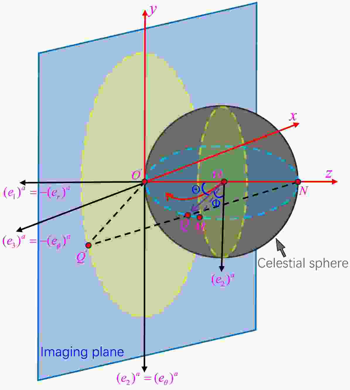
$ (e_{0})^a $ is the timelike vector representing the observer's four-velocity;$ (e_{1})^a $ is in the opposite direction of the observer's spatial radial basis$ (e_{r})^a $ and points toward the black hole center.$ g_{ab} $ is the metric defined by Eq. (8). It is important to note that the choice of tetrad is not unique, and different tetrads are related by Lorentz transformations. Using the tetrad (31)−(34) and the method of stereographic projection, we can obtain the black hole shadow image.In Fig. 1, we illustrate the method of stereographic projection [80]. The observer is located at point O, and the red arrow originating from O represents the direction of photon propagation. The vector
$ \overrightarrow{OQ} $ is the tangent vector to the null geodesic passing through point O, representing the photon's three-momentum. Its geometric meaning is the projection of the tangent vector of the null geodesic at point O onto the observer's three-dimensional subspace. The celestial sphere is a three-dimensional sphere centered at O with radius$ |\overrightarrow{OQ}| $ . We set the origin of the tetrad (31)−(34) as$ O^\prime $ and place$ O^\prime $ on the celestial sphere, i.e.,$ |OO^\prime| = |\overrightarrow{OQ}| $ is the radius of the celestial sphere. Extending$ |O^\prime O| $ , it intersects the celestial sphere at point N, such that$ |O^\prime N| $ becomes the diameter of the celestial sphere and is collinear with the basis vector$ (e_{1})^a $ . The blue rectangular plane passing through point$ O^\prime $ is the imaging plane, which is tangent to the celestial sphere. The line connecting N and Q intersects the imaging plane at point$ Q^\prime $ , and the projection of the vector$ |\overrightarrow{OQ}| $ onto the imaging plane is represented by the vector$ |\overrightarrow{O^\prime Q^\prime}| $ . To describe the direction of the photon source as seen by the observer, we introduce celestial coordinates$ (\Theta, \Phi) $ , where Θ is the angle between$ \overrightarrow{OQ} $ and$ (e_1)^a $ , and Φ is the angle between$ \overrightarrow{OQ} $ and$ (e_2)^a $ .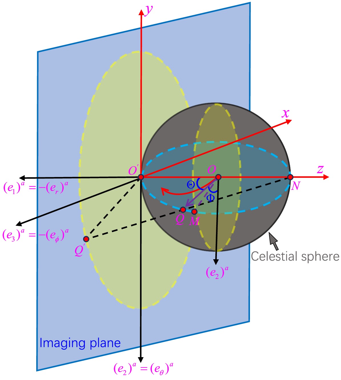
Figure 1. (color online) ZAMO tetrad and celestial coordinates
$ (\Theta, \Phi) $ based on the method of stereographic projection. The gray sphere represents the three-dimensional subspace of the observer, with$ (e_{1})^a $ pointing toward the center of the black hole. The blue plane is the imaging plane.Utilizing spherical coordinates, under the frame (31)−(34), the tangent vector of the null geodesic can be expressed as
$ \begin{aligned}[b] U^a =\;& |\overrightarrow{OQ}|[-(e_{0})^a+\cos\Theta(e_{1})^a\\&+\sin\Theta\cos\Phi(e_{2})^a+\sin\Theta\sin\Phi(e_{3})^a], \end{aligned} $
(35) where the negative sign in front of
$ -(e_{0})^a $ ensures that the tangent vector is a past directed null vector. Additionally, since the photon trajectory is independent of its energy, we set the photon energy to be 1, i.e.,$ |\overrightarrow{OQ}| = 1 $ . On the other hand, for each photon path$ \gamma(\tau) $ , the coordinates$ (t,r,\theta,\phi) $ are functions of τ, and the general form of its tangent vector is$ U^a = \dot{t}\left(\frac{\partial}{\partial t }\right)^a+\dot{r}\left(\frac{\partial}{\partial r}\right)^a+\dot{\theta}\left(\frac{\partial}{\partial \theta}\right)^a+\dot{\phi}\left(\frac{\partial}{\partial \phi}\right)^a. $
(36) Eqs. (31)−(36) show that the photon four-momentum corresponds one-to-one with the spherical coordinates. Once the photon four-momentum is known, the spherical coordinates can be determined; conversely, if the spherical coordinates are known, the photon four-momentum can be determined, through coordinate transformation. Therefore, by combining the observer's position, we can determine the initial values of the photon motion equations
$ \left.(x^\mu,p_\mu)\right|_o $ . In the ZAMO frame, the photon's four-momentum is given by$ p_b = p_a e_{b}{}^{a} $ , where$ e_{b}{}^{a} $ is defined in Eqs. (31)−(34), and$ p_a $ is determined by Eqs. (17)−(20). Let the components of$ p^c $ in the ZAMO frame be$ p^\mu $ , which satisfies the relation$ p^c = p_b g^{bc} $ , where$ g^{bc} $ is the metric defined in Eq. (8). According to [81], the relationship between the spherical coordinates and the photon four-momentum are$ \cos\Theta = \frac{p^{1}}{p^{0}},\quad \tan\Phi = \frac{p^{3}}{p^{2}}. $
(37) Additionally, to obtain the black hole shadow image, it is necessary to relate the spherical coordinates
$ (\Theta, \Phi) $ to the points$ (x, y) $ on the imaging plane in the Cartesian coordinate system. The correspondence depends on the camera model used. In this study, we choose the wide-angle fisheye camera model. A Cartesian coordinate system is established on the imaging plane with$ O^\prime $ as the origin, and the projection coordinates of point A on this plane are given by$ x_Q = -2\tan\left(\frac{\Theta}{2}\right)\sin\Phi,\quad y_Q = -2\tan\left(\frac{\Theta}{2}\right)\cos\Phi. $
(38) For the rotating black hole in the KR gravity, the expressions for the spherical coordinates are
$ \Theta(r_p) = \arccos\left[\frac{\sqrt{A} \sqrt{(a^2+r^2)^2 - a^2\Delta - \Delta\eta(r_p) - 2B + (a^2 - \Delta)\xi^2(r_p)}}{A - B}\right], $
(39) $ \Phi(r_p) = \arctan\left[\frac{\sqrt{\Sigma^2}\xi(r_p)}{\sqrt{A\sin^2\theta}\sqrt{a^2\cos^2\theta + \eta(r_p) - \cot^2\theta\xi^2(r_p)}}\right], $
(40) where
$ A = (a^2 + r^2)^2 - a^2\Delta\sin^2\theta,\quad B = a(a^2 + r^2 - \Delta)\xi(r_p), $
(41) $ r_p $ is the photon sphere radius, satisfying condition (25). Accordingly, we can plot the shadow images of a rotating black hole in KR gravity. This paper will study the effects of the Lorentz symmetry violation parameters$ {\cal{G}} $ , λ, and the rotation parameter a on the shadow images.As shown in Fig. 2(a), we fix the spontaneous Lorentz symmetry violation parameters
$ \lambda = 0.1 $ and$ {\cal{G}} = 0.9 $ , and vary the rotation parameter a. The red, green, blue, and orange shadow images correspond to$ a = 0.1, 0.4, 0.7, 0.9 $ , respectively. When$ a \to 0 $ , the shadow appears as a perfect circle and is symmetric about the x-axis. As a increases, the shadow image gradually shifts in the positive x direction, with the curvature on the left side slightly decreasing and flattening, but the variation in a has little significant effect on the size of the shadow. As shown in Fig. 2(b), we fix$ a = 0.3 $ and$ {\cal{G}} = 0.9 $ , and vary λ. The red, green, blue, and orange shadow images correspond to$ \lambda = 0.1, 0.4, 0.7, 0.9 $ , respectively. While λ has little effect on the shape of the shadow, as λ increases, the shadow size significantly decreases and shifts in the positive x direction. As shown in Fig. 2(c), we fix$ a = 0.3 $ and$ \lambda = 0.9 $ , and the red, green, blue, and orange shadow images correspond to$ {\cal{G}} = 0.1, 0.4, 0.7, 0.9 $ , respectively. The effect of$ {\cal{G}} $ on the shape and size of the shadow is similar to that of λ. As$ {\cal{G}} $ increases, the shadow size decreases, and the left side of the shadow image flattens and shifts in the positive x direction. The differences between these images will be discussed in the following sections, which may serve as a basis for distinguishing rotating black holes in KR gravity from other spacetimes.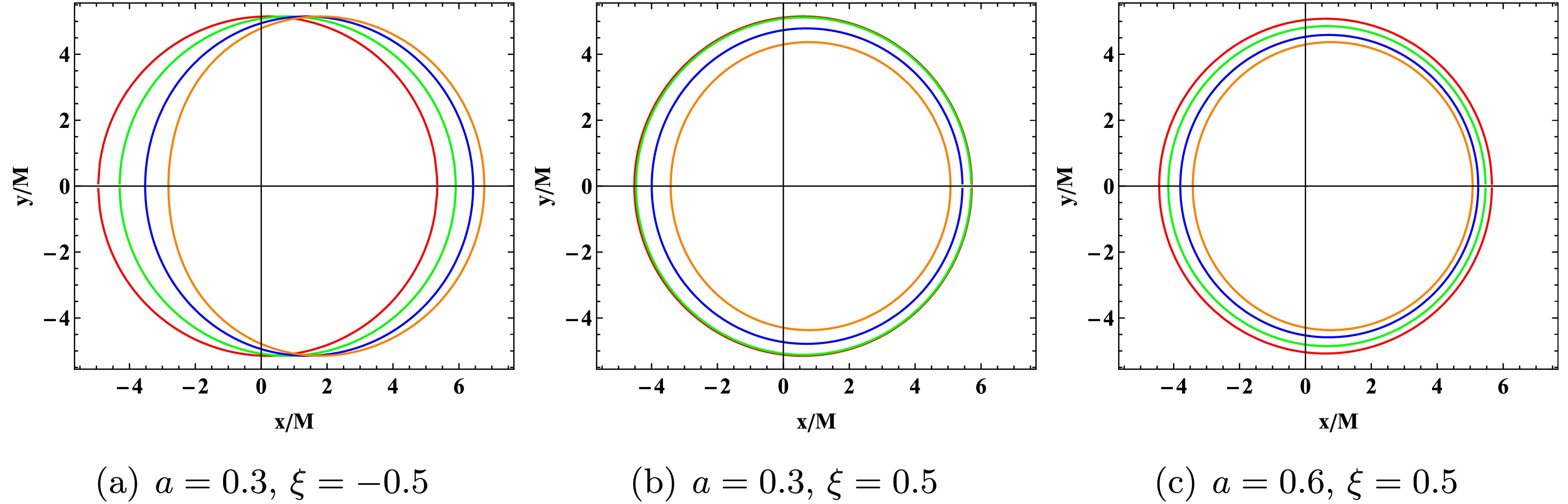
Figure 2. (color online) Shadow images of a rotating black hole in KR gravity and their relationships with parameters a, λ, and
$ {\cal{G}} $ are investigated. In the left panel, the red, green, blue, and orange shadow images correspond to$ a = 0.1,\, 0.4,\, 0.7,\, 0.9 $ , respectively. In the middle panel, the red, green, blue, and orange shadow images correspond to$ \lambda = 0.1,\, 0.4,\, 0.7,\, 0.9 $ , respectively. In the right panel, the red, green, blue, and orange shadow images correspond to$ {\cal{G}} = 0.1,\, 0.4,\, 0.7,\, 0.9 $ , respectively. The fixed parameters include the black hole mass$ M = 1 $ , observer distance$ r_o = 100 $ , and observer inclination angle$ \theta_o = 90^{\circ} $ .To effectively describe the effects of parameters on the size and shape of the black hole shadow, we define two observable physical quantities: the size and the deviation from the circularity
$ R_d = \frac{(x_t - x_r)^2 + y_t^2}{2|x_t - x_r|},\quad \delta_d = \frac{|x_{\tilde{l}} - x_l|}{R_d}. $
(42) Here,
$ R_d $ is the radius of the reference circle passing through the top, bottom, and rightmost points of the black hole shadow, used to approximately reflect the size of the shadow;$ \delta_d $ represents the degree of deviation from the circularity. In particular, the five reference points involved in Eq. (42) are shown in Fig. 3, where$ (x_t, y_t) $ ,$ (x_b, y_b) $ ,$ (x_r, 0) $ ,$ (x_l, 0) $ , and$ (x_{\tilde{l}}, 0) $ correspond to the top, bottom, rightmost, and leftmost points of the black hole shadow, and the leftmost point of the reference circle, respectively. When$ x_l \neq x_{\tilde{l}} $ ,$ \delta_d \neq 0 $ . This phenomenon occurs because, for rotating black holes, the radii of the innermost unstable circular orbits for prograde and retrograde photons are unequal. The right endpoint of the black hole shadow,$ (x_r, 0) $ , corresponds to the unstable retrograde circular orbit observed by an observer in the equatorial plane, whose center is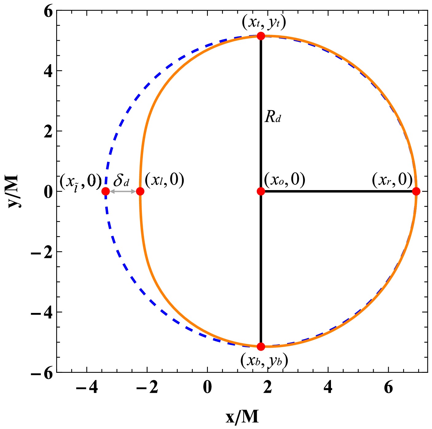
Figure 3. (color online) Black hole shadow and the reference circle. The orange contour represents the black hole shadow, and the blue contour represents the reference circle. The radius of the reference circle is
$ R_d $ , and the absolute value of the difference in the x-coordinate between the reference circle and the left endpoint of the black hole shadow is$ \delta_d $ .$ x_{o} = \frac{x_{r}^{2}-x_{t}^{2}-y_{t}^{2}}{2(x_{r}-x_{t})}, $
(43) and coincides with the center of the reference circle. In Fig. 4, we show the effects of the parameters
$ {\cal{G}} $ , λ, and a in KR gravity on$ R_d $ and$ \delta_d $ . From the figure, we can observe that, with other parameters fixed, as a increases, both$ R_d $ and$ \delta_d $ show a monotonic increase, although the increase in$ R_d $ is small. As λ and$ {\cal{G}} $ increase,$ R_d $ decreases gradually, while$ \delta_d $ increases. These trends are consistent with the results in Fig. 2, but they are more intuitive.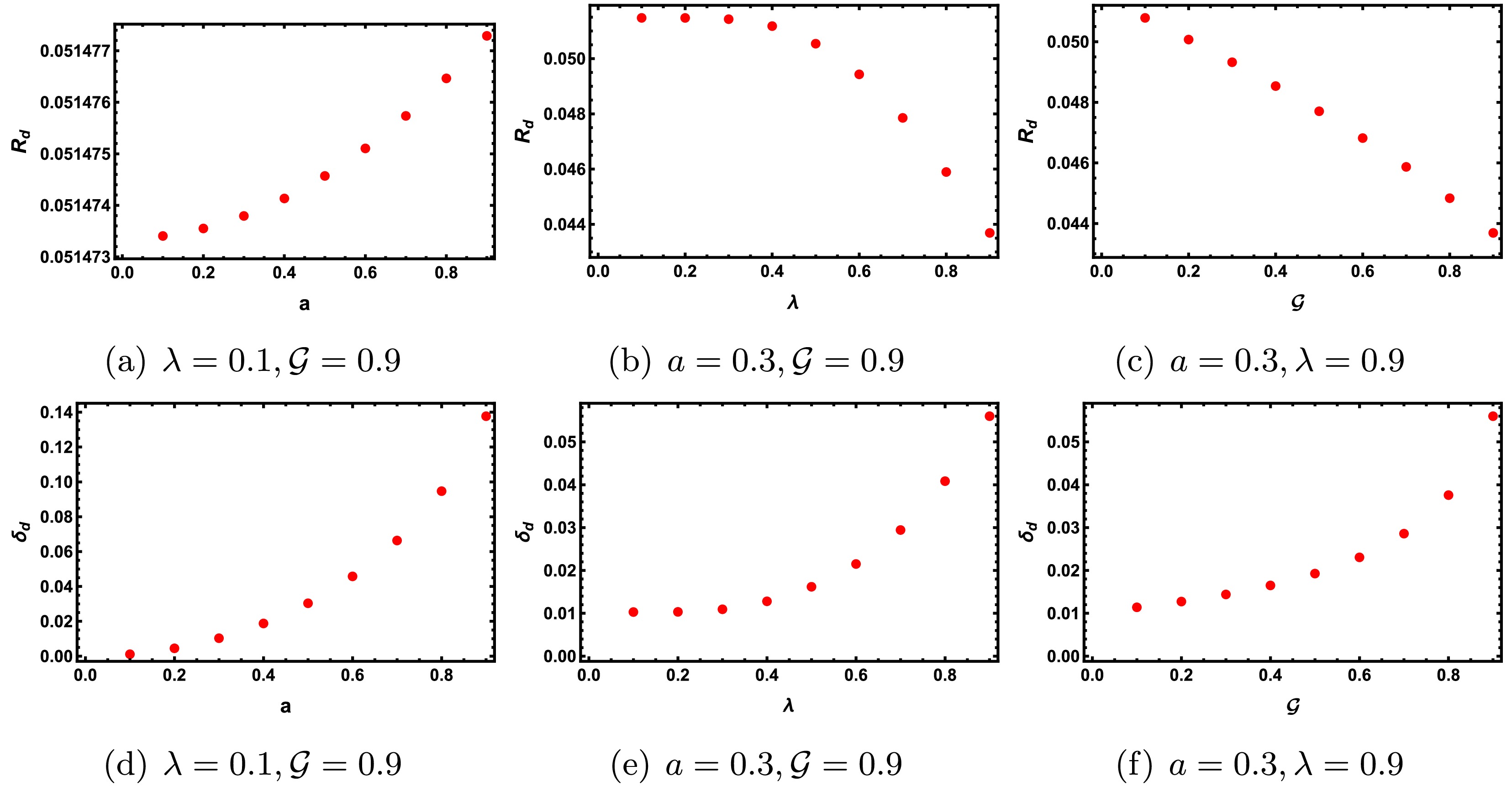
Figure 4. (color online) Relationship between the black hole shadow size
$ R_d $ and the deviation from the circularity$ \delta_d $ with respect to parameter variations in KR gravity. The first column fixes$ \lambda = 0.1 $ ,$ {\cal{G}} = 0.9 $ ; the second column fixes$ a = 0.3 $ ,$ {\cal{G}} = 0.9 $ ; the third column fixes$ a = 0.3 $ ,$ \lambda = 0.9 $ , with the other parameters varying from$ 0.1 $ to$ 0.9 $ in equal intervals.In astronomical observations, the physical quantity used to reflect the size of the black hole shadow is the angular diameter
$ {\cal{D}} = 2 \tilde{R}_d \frac{{\cal{M}}}{D_o} $ , where$ D_o $ is the distance between the black hole and the observer,$ \tilde{R}_d $ is the shadow radius at the black hole position on the screen, which is related to the shadow size$ R_d $ and can be calculated through a simple geometric relation, and$ {\cal{M}} $ is the black hole mass. According to the references [82], when the black hole is far from the observer, the angular diameter can be quantitatively expressed as$ {\cal{D}} = 2 \times 9.87098\tilde{R}_{d}\left(\frac{{\cal{M}}}{M_{\odot}}\right)\left(\frac{1\;{\rm kpc}}{D_{o}}\right)\mathrm{\mu as}. $
(44) In Fig. 5, we show the estimated ranges of the angular diameter
$ {\cal{D}} $ of the shadows of Sgr A* and M87*. The first row corresponds to Sgr A*, and the second row corresponds to M87*. The orange solid line represents the$ 1\sigma $ confidence interval of$ {\cal{D}} $ , the purple dashed line represents the$ 2\sigma $ confidence interval, and the red line segments represent the estimated range, with the endpoints marked with bold black short lines. The results indicate that when$ a = 0.3,\; {\cal{G}} = 0.9 $ , as λ increases, the angular diameter of both Sgr A* and M87* decreases. Specifically, for Sgr A*, when$ \lambda \lt 0.6 $ , the decrease in$ {\cal{D}}_{\mathrm{Sgr A^*}} $ is relatively slow, while for$ \lambda \gt 0.6 $ , the decrease accelerates significantly; for M87*, the critical point for this change is around$ \lambda = 0.5 $ . On the other hand, when$ a = 0.3,\; \lambda = 0.9 $ , as$ {\cal{G}} $ increases, the angular diameter of both Sgr A* and M87 also decreases, but the decrease in$ {\cal{D}}_{\mathrm{M87^*}} $ is more pronounced. In all of the above cases, the estimated range of$ {\cal{D}} $ is within the$ 1\sigma $ confidence interval. It should be noted that several studies have already constrained the possible ranges of λ and$ {\cal{G}} $ . For instance, Ref. [76] obtained an upper bound of$ {\cal{G}}<2.8\times10^{-3}\;{\rm km}^2 $ under the condition$ \lambda = 1 $ by analyzing Mercury’s perihelion precession, while Ref. [83] constrained the parameter space to$ 0<\lambda \ll 1 $ through the tests of light deflection and Shapiro time delay. In this study, however, within the framework of geometric units we adopt values$ {\cal{G}} $ and λ for the purpose of demonstrating the qualitative trends of their effects, rather than representing physically realistic parameters. This choice is not contradictory, provided that the estimated ranges of the shadow angular diameter$ {\cal{D}} $ remain within the$ 2\sigma $ confidence intervals of the observational data.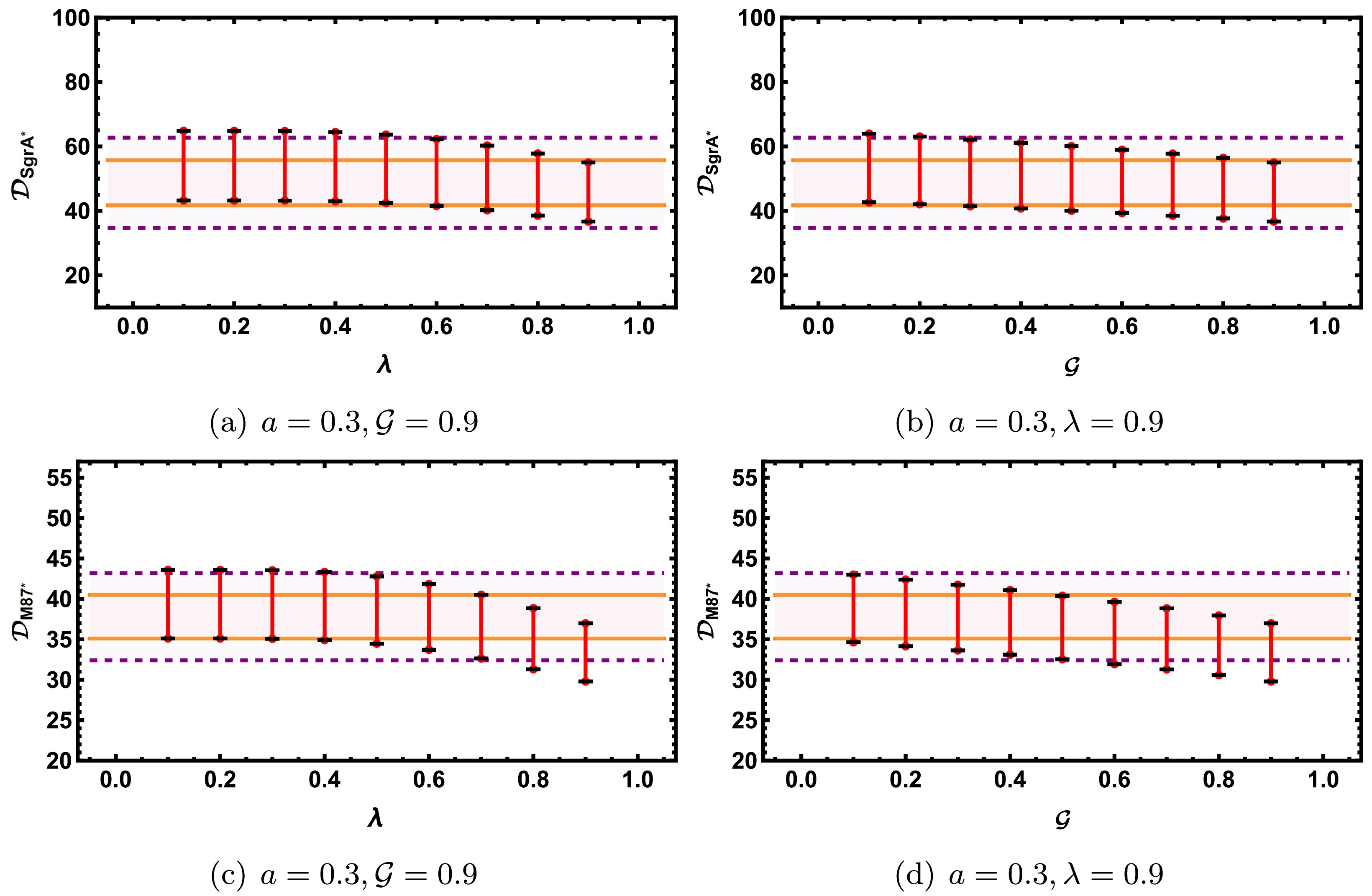
Figure 5. (color online) The estimated ranges of the shadow angular diameter
$ {\cal{D}} $ for Sgr A* and M87. The orange solid line and the purple dashed line represent the$ 1\sigma $ and$ 2\sigma $ confidence intervals, respectively, while the red line segments represent the estimated ranges, with corresponding parameters varying from$ 0.1 $ to$ 0.9 $ in equal intervals. -
To obtain the shadow of the rotating black hole in KR gravity, it is necessary to study the photon sphere of the black hole. The photon sphere is a special surface located outside the event horizon. Once a photon enters the photon sphere, it is captured by the black hole and cannot reach an observer at infinity. Only light outside the photon sphere can reach the observer. Therefore, the size and boundary of the black hole shadow are actually determined by the radius of the photon sphere. By choosing a coordinate system such that the value of θ for the null geodesic is always
$ \pi/2 $ (i.e., the photon always remains in the equatorial plane), the radial equation can be rewritten as$ \dot{r}^2+V_{\rm eff}(r) = 0, $
(23) where
$ V_{\rm eff}(r) = -\frac{R(r)}{2r^4} = -\frac{\left[{\cal{E}}(r^2+a^2)-a{\cal{L}}\right]^2-\Delta\left[{\cal{C}}+({\cal{L}}-a{\cal{E}})^2\right]}{2r^4} . $
(24) where
$ V_{\rm eff} $ is the effective potential for the photon. If the photon captured by the black hole is in an unstable orbit, it may escape after several orbits around the black hole; if it is in a stable orbit, it will be bound for a long time. The properties of these orbits are determined by the effective potential. Photons emitted from the light source or accretion disk may get trapped in the local region near the event horizon, where some photons fall into the horizon, while others escape to infinity. This phenomenon forms the black hole shadow, whose boundary is surrounded by a luminous massless sphere [79], called the photon sphere. The radius of the photon sphere can be derived from the conditions$ \dot{r}(\tau) = 0 $ and$ \ddot{r}(\tau) = 0 $ . According to Eqs. (18) and (24), this condition is equivalent to$ R(r) = 0,\quad \frac{\partial R(r)}{\partial r} = 0, $
(25) or
$ V_{\rm eff}(r) = 0,\quad \frac{\partial V_{\rm eff}(r)}{\partial r} = 0. $
(26) For unstable orbits,
$ V\mathrm{_{eff}}(r) $ must also satisfy the condition for a maximum value:$ \frac{\partial^2V_{\mathrm{eff}}(r)}{\partial r^2} < 0 $ . To solve the system of Eq. (26), define the impact parameters$ \xi \equiv \frac{{\cal{L}}}{{\cal{E}}}, \quad \eta \equiv \frac{{\cal{C}}}{{\cal{E}}^{2}}. $
(27) Solving Eq. (26) based on this gives
$ \xi = \frac{r^{2}+a^{2}}{a} - \frac{2r\left[r^{2}+a^{2}-2Mr+{\cal{G}} r^{\frac{2(\lambda-1)}{\lambda}}\right]} {a\left[r-M+{\cal{G}}\left(1-\frac{1}{\lambda}\right)r^{1-\frac{2}{\lambda}}\right]}, $
(28) $ \begin{aligned}[b] \eta =\;& \frac{r^2}{a^2\Delta^{\prime}} \Big[16\Delta\big(a^2-\Delta\big) - r^2(\Delta^{\prime})^2 + 8r\Delta\Delta^{\prime}\Big] \\ =\;& -\Bigg\{\lambda^2r^{3+\frac{4}{\lambda}}\Big[r\big(r-3M\big)^2 - 4Ma^2\Big] + r^6{\cal{G}}^2\big(\lambda+1\big)^2 \\ & + 2{\cal{G}}\lambda r^{4+\frac{2}{\lambda}} \Big[2a^2 + r(r-3M)(\lambda+1)\Big]\Bigg\} \\&\times\Big[ar{\cal{G}}(\lambda-1) + a\lambda r^{\frac{2}{\lambda}}(r-M)\Big]^{-2}, \end{aligned} $
(29) where
$ \Delta^{\prime} $ represents the derivative with respect to the radial distance r. Since$ \Theta \geq 0 $ in Eq. (19), the impact parameters satisfy$ \eta-\xi^2\cot\theta^2+a^2\cos^2\theta\geq 0. $
(30) This condition defines the region where photons can exist.
The geodesic differential Eqs. (17)−(20) are insufficient to fully describe the motion of photons. To obtain the black hole shadow image, it is necessary to determine the integration constants. For this, we choose the zero angular momentum observer (ZAMO). Suppose the observer is located at
$ (t_o, r_o, \theta_o, \phi_o) $ , and within its neighborhood, there exists a local orthonormal tetrad defined as$ (e_{0})^a = \left(\sqrt{\frac{-g_{\phi\phi}}{g_{tt}g_{\phi\phi}-g_{t\phi}^{2}}},0,0,\frac{-g_{t\phi}}{g_{\phi\phi}}\sqrt{\frac{-g_{\phi\phi}}{g_{tt}g_{\phi\phi}-g_{t\phi}^{2}}}\right), $
(31) $ (e_{1})^a = \left(0,\frac{-1}{\sqrt{g_{rr}}},0,0\right), $
(32) $ (e_{2})^a = \left(0,0,\frac{1}{\sqrt{g_{\theta\theta}}},0\right), $
(33) $ (e_{3})^a = \left(0,0,0,\frac{-1}{\sqrt{g_{\phi\phi}}}\right), $
(34) where
$ (e_{0})^a $ is the timelike vector representing the observer's four-velocity;$ (e_{1})^a $ is in the opposite direction of the observer's spatial radial basis$ (e_{r})^a $ and points toward the black hole center.$ g_{ab} $ is the metric defined by Eq. (8). It is important to note that the choice of tetrad is not unique, and different tetrads are related by Lorentz transformations. Using the tetrad (31)−(34) and the method of stereographic projection, we can obtain the black hole shadow image.In Fig. 1, we illustrate the method of stereographic projection [80]. The observer is located at point O, and the red arrow originating from O represents the direction of photon propagation. The vector
$ \overrightarrow{OQ} $ is the tangent vector to the null geodesic passing through point O, representing the photon's three-momentum. Its geometric meaning is the projection of the tangent vector of the null geodesic at point O onto the observer's three-dimensional subspace. The celestial sphere is a three-dimensional sphere centered at O with radius$ |\overrightarrow{OQ}| $ . We set the origin of the tetrad (31)−(34) as$ O^\prime $ and place$ O^\prime $ on the celestial sphere, i.e.,$ |OO^\prime| = |\overrightarrow{OQ}| $ is the radius of the celestial sphere. Extending$ |O^\prime O| $ , it intersects the celestial sphere at point N, such that$ |O^\prime N| $ becomes the diameter of the celestial sphere and is collinear with the basis vector$ (e_{1})^a $ . The blue rectangular plane passing through point$ O^\prime $ is the imaging plane, which is tangent to the celestial sphere. The line connecting N and Q intersects the imaging plane at point$ Q^\prime $ , and the projection of the vector$ |\overrightarrow{OQ}| $ onto the imaging plane is represented by the vector$ |\overrightarrow{O^\prime Q^\prime}| $ . To describe the direction of the photon source as seen by the observer, we introduce celestial coordinates$ (\Theta, \Phi) $ , where Θ is the angle between$ \overrightarrow{OQ} $ and$ (e_1)^a $ , and Φ is the angle between$ \overrightarrow{OQ} $ and$ (e_2)^a $ .
Figure 1. (color online) ZAMO tetrad and celestial coordinates
$ (\Theta, \Phi) $ based on the method of stereographic projection. The gray sphere represents the three-dimensional subspace of the observer, with$ (e_{1})^a $ pointing toward the center of the black hole. The blue plane is the imaging plane.Utilizing spherical coordinates, under the frame (31)−(34), the tangent vector of the null geodesic can be expressed as
$ \begin{aligned}[b] U^a =\;& |\overrightarrow{OQ}|[-(e_{0})^a+\cos\Theta(e_{1})^a\\&+\sin\Theta\cos\Phi(e_{2})^a+\sin\Theta\sin\Phi(e_{3})^a], \end{aligned} $
(35) where the negative sign in front of
$ -(e_{0})^a $ ensures that the tangent vector is a past directed null vector. Additionally, since the photon trajectory is independent of its energy, we set the photon energy to be 1, i.e.,$ |\overrightarrow{OQ}| = 1 $ . On the other hand, for each photon path$ \gamma(\tau) $ , the coordinates$ (t,r,\theta,\phi) $ are functions of τ, and the general form of its tangent vector is$ U^a = \dot{t}\left(\frac{\partial}{\partial t }\right)^a+\dot{r}\left(\frac{\partial}{\partial r}\right)^a+\dot{\theta}\left(\frac{\partial}{\partial \theta}\right)^a+\dot{\phi}\left(\frac{\partial}{\partial \phi}\right)^a. $
(36) Eqs. (31)−(36) show that the photon four-momentum corresponds one-to-one with the spherical coordinates. Once the photon four-momentum is known, the spherical coordinates can be determined; conversely, if the spherical coordinates are known, the photon four-momentum can be determined, through coordinate transformation. Therefore, by combining the observer's position, we can determine the initial values of the photon motion equations
$ \left.(x^\mu,p_\mu)\right|_o $ . In the ZAMO frame, the photon's four-momentum is given by$ p_b = p_a e_{b}{}^{a} $ , where$ e_{b}{}^{a} $ is defined in Eqs. (31)−(34), and$ p_a $ is determined by Eqs. (17)−(20). Let the components of$ p^c $ in the ZAMO frame be$ p^\mu $ , which satisfies the relation$ p^c = p_b g^{bc} $ , where$ g^{bc} $ is the metric defined in Eq. (8). According to [81], the relationship between the spherical coordinates and the photon four-momentum are$ \cos\Theta = \frac{p^{1}}{p^{0}},\quad \tan\Phi = \frac{p^{3}}{p^{2}}. $
(37) Additionally, to obtain the black hole shadow image, it is necessary to relate the spherical coordinates
$ (\Theta, \Phi) $ to the points$ (x, y) $ on the imaging plane in the Cartesian coordinate system. The correspondence depends on the camera model used. In this study, we choose the wide-angle fisheye camera model. A Cartesian coordinate system is established on the imaging plane with$ O^\prime $ as the origin, and the projection coordinates of point A on this plane are given by$ x_Q = -2\tan\left(\frac{\Theta}{2}\right)\sin\Phi,\quad y_Q = -2\tan\left(\frac{\Theta}{2}\right)\cos\Phi. $
(38) For the rotating black hole in the KR gravity, the expressions for the spherical coordinates are
$ \Theta(r_p) = \arccos\left[\frac{\sqrt{A} \sqrt{(a^2+r^2)^2 - a^2\Delta - \Delta\eta(r_p) - 2B + (a^2 - \Delta)\xi^2(r_p)}}{A - B}\right], $
(39) $ \Phi(r_p) = \arctan\left[\frac{\sqrt{\Sigma^2}\xi(r_p)}{\sqrt{A\sin^2\theta}\sqrt{a^2\cos^2\theta + \eta(r_p) - \cot^2\theta\xi^2(r_p)}}\right], $
(40) where
$ A = (a^2 + r^2)^2 - a^2\Delta\sin^2\theta,\quad B = a(a^2 + r^2 - \Delta)\xi(r_p), $
(41) $ r_p $ is the photon sphere radius, satisfying condition (25). Accordingly, we can plot the shadow images of a rotating black hole in KR gravity. This paper will study the effects of the Lorentz symmetry violation parameters$ {\cal{G}} $ , λ, and the rotation parameter a on the shadow images.As shown in Fig. 2(a), we fix the spontaneous Lorentz symmetry violation parameters
$ \lambda = 0.1 $ and$ {\cal{G}} = 0.9 $ , and vary the rotation parameter a. The red, green, blue, and orange shadow images correspond to$ a = 0.1, 0.4, 0.7, 0.9 $ , respectively. When$ a \to 0 $ , the shadow appears as a perfect circle and is symmetric about the x-axis. As a increases, the shadow image gradually shifts in the positive x direction, with the curvature on the left side slightly decreasing and flattening, but the variation in a has little significant effect on the size of the shadow. As shown in Fig. 2(b), we fix$ a = 0.3 $ and$ {\cal{G}} = 0.9 $ , and vary λ. The red, green, blue, and orange shadow images correspond to$ \lambda = 0.1, 0.4, 0.7, 0.9 $ , respectively. While λ has little effect on the shape of the shadow, as λ increases, the shadow size significantly decreases and shifts in the positive x direction. As shown in Fig. 2(c), we fix$ a = 0.3 $ and$ \lambda = 0.9 $ , and the red, green, blue, and orange shadow images correspond to$ {\cal{G}} = 0.1, 0.4, 0.7, 0.9 $ , respectively. The effect of$ {\cal{G}} $ on the shape and size of the shadow is similar to that of λ. As$ {\cal{G}} $ increases, the shadow size decreases, and the left side of the shadow image flattens and shifts in the positive x direction. The differences between these images will be discussed in the following sections, which may serve as a basis for distinguishing rotating black holes in KR gravity from other spacetimes.
Figure 2. (color online) Shadow images of a rotating black hole in KR gravity and their relationships with parameters a, λ, and
$ {\cal{G}} $ are investigated. In the left panel, the red, green, blue, and orange shadow images correspond to$ a = 0.1,\, 0.4,\, 0.7,\, 0.9 $ , respectively. In the middle panel, the red, green, blue, and orange shadow images correspond to$ \lambda = 0.1,\, 0.4,\, 0.7,\, 0.9 $ , respectively. In the right panel, the red, green, blue, and orange shadow images correspond to$ {\cal{G}} = 0.1,\, 0.4,\, 0.7,\, 0.9 $ , respectively. The fixed parameters include the black hole mass$ M = 1 $ , observer distance$ r_o = 100 $ , and observer inclination angle$ \theta_o = 90^{\circ} $ .To effectively describe the effects of parameters on the size and shape of the black hole shadow, we define two observable physical quantities: the size and the deviation from the circularity
$ R_d = \frac{(x_t - x_r)^2 + y_t^2}{2|x_t - x_r|},\quad \delta_d = \frac{|x_{\tilde{l}} - x_l|}{R_d}. $
(42) Here,
$ R_d $ is the radius of the reference circle passing through the top, bottom, and rightmost points of the black hole shadow, used to approximately reflect the size of the shadow;$ \delta_d $ represents the degree of deviation from the circularity. In particular, the five reference points involved in Eq. (42) are shown in Fig. 3, where$ (x_t, y_t) $ ,$ (x_b, y_b) $ ,$ (x_r, 0) $ ,$ (x_l, 0) $ , and$ (x_{\tilde{l}}, 0) $ correspond to the top, bottom, rightmost, and leftmost points of the black hole shadow, and the leftmost point of the reference circle, respectively. When$ x_l \neq x_{\tilde{l}} $ ,$ \delta_d \neq 0 $ . This phenomenon occurs because, for rotating black holes, the radii of the innermost unstable circular orbits for prograde and retrograde photons are unequal. The right endpoint of the black hole shadow,$ (x_r, 0) $ , corresponds to the unstable retrograde circular orbit observed by an observer in the equatorial plane, whose center is
Figure 3. (color online) Black hole shadow and the reference circle. The orange contour represents the black hole shadow, and the blue contour represents the reference circle. The radius of the reference circle is
$ R_d $ , and the absolute value of the difference in the x-coordinate between the reference circle and the left endpoint of the black hole shadow is$ \delta_d $ .$ x_{o} = \frac{x_{r}^{2}-x_{t}^{2}-y_{t}^{2}}{2(x_{r}-x_{t})}, $
(43) and coincides with the center of the reference circle. In Fig. 4, we show the effects of the parameters
$ {\cal{G}} $ , λ, and a in KR gravity on$ R_d $ and$ \delta_d $ . From the figure, we can observe that, with other parameters fixed, as a increases, both$ R_d $ and$ \delta_d $ show a monotonic increase, although the increase in$ R_d $ is small. As λ and$ {\cal{G}} $ increase,$ R_d $ decreases gradually, while$ \delta_d $ increases. These trends are consistent with the results in Fig. 2, but they are more intuitive.
Figure 4. (color online) Relationship between the black hole shadow size
$ R_d $ and the deviation from the circularity$ \delta_d $ with respect to parameter variations in KR gravity. The first column fixes$ \lambda = 0.1 $ ,$ {\cal{G}} = 0.9 $ ; the second column fixes$ a = 0.3 $ ,$ {\cal{G}} = 0.9 $ ; the third column fixes$ a = 0.3 $ ,$ \lambda = 0.9 $ , with the other parameters varying from$ 0.1 $ to$ 0.9 $ in equal intervals.In astronomical observations, the physical quantity used to reflect the size of the black hole shadow is the angular diameter
$ {\cal{D}} = 2 \tilde{R}_d \frac{{\cal{M}}}{D_o} $ , where$ D_o $ is the distance between the black hole and the observer,$ \tilde{R}_d $ is the shadow radius at the black hole position on the screen, which is related to the shadow size$ R_d $ and can be calculated through a simple geometric relation, and$ {\cal{M}} $ is the black hole mass. According to the references [82], when the black hole is far from the observer, the angular diameter can be quantitatively expressed as$ {\cal{D}} = 2 \times 9.87098\tilde{R}_{d}\left(\frac{{\cal{M}}}{M_{\odot}}\right)\left(\frac{1\;{\rm kpc}}{D_{o}}\right)\mathrm{\mu as}. $
(44) In Fig. 5, we show the estimated ranges of the angular diameter
$ {\cal{D}} $ of the shadows of Sgr A* and M87*. The first row corresponds to Sgr A*, and the second row corresponds to M87*. The orange solid line represents the$ 1\sigma $ confidence interval of$ {\cal{D}} $ , the purple dashed line represents the$ 2\sigma $ confidence interval, and the red line segments represent the estimated range, with the endpoints marked with bold black short lines. The results indicate that when$ a = 0.3,\; {\cal{G}} = 0.9 $ , as λ increases, the angular diameter of both Sgr A* and M87* decreases. Specifically, for Sgr A*, when$ \lambda < 0.6 $ , the decrease in$ {\cal{D}}_{\mathrm{Sgr A^*}} $ is relatively slow, while for$ \lambda > 0.6 $ , the decrease accelerates significantly; for M87*, the critical point for this change is around$ \lambda = 0.5 $ . On the other hand, when$ a = 0.3,\; \lambda = 0.9 $ , as$ {\cal{G}} $ increases, the angular diameter of both Sgr A* and M87 also decreases, but the decrease in$ {\cal{D}}_{\mathrm{M87^*}} $ is more pronounced. In all of the above cases, the estimated range of$ {\cal{D}} $ is within the$ 1\sigma $ confidence interval. It should be noted that several studies have already constrained the possible ranges of λ and$ {\cal{G}} $ . For instance, Ref. [76] obtained an upper bound of$ {\cal{G}}<2.8\times10^{-3}\;{\rm km}^2 $ under the condition$ \lambda = 1 $ by analyzing Mercury’s perihelion precession, while Ref. [83] constrained the parameter space to$ 0<\lambda \ll 1 $ through the tests of light deflection and Shapiro time delay. In this study, however, within the framework of geometric units we adopt values$ {\cal{G}} $ and λ for the purpose of demonstrating the qualitative trends of their effects, rather than representing physically realistic parameters. This choice is not contradictory, provided that the estimated ranges of the shadow angular diameter$ {\cal{D}} $ remain within the$ 2\sigma $ confidence intervals of the observational data.
Figure 5. (color online) The estimated ranges of the shadow angular diameter
$ {\cal{D}} $ for Sgr A* and M87. The orange solid line and the purple dashed line represent the$ 1\sigma $ and$ 2\sigma $ confidence intervals, respectively, while the red line segments represent the estimated ranges, with corresponding parameters varying from$ 0.1 $ to$ 0.9 $ in equal intervals. -
To obtain the shadow of the rotating black hole in KR gravity, it is necessary to study the photon sphere of the black hole. The photon sphere is a special surface located outside the event horizon. Once a photon enters the photon sphere, it will be captured by the black hole and cannot reach an observer at infinity. Only light outside the photon sphere can reach the observer. Therefore, the size and boundary of the black hole shadow are actually determined by the radius of the photon sphere. By choosing a coordinate system such that the value of θ for the null geodesic is always
$ \pi/2 $ (i.e., the photon always remains in the equatorial plane), the radial equation can be rewritten as$ \dot{r}^2+V_{eff}(r) = 0, $

(23) where
$ V_{eff}(r) = -\frac{R(r)}{2r^4} = -\frac{\left[{\cal{E}}(r^2+a^2)-a{\cal{L}}\right]^2-\Delta\left[{\cal{C}}+({\cal{L}}-a{\cal{E}})^2\right]}{2r^4} . $

(24) Here, the term of
$ V_{eff} $ is the effective potential for the photon. If the photon captured by the black hole is in an unstable orbit, it may escape after several orbits around the black hole; if it is in a stable orbit, it will be bound for a long time. The properties of these orbits are determined by the effective potential. Photons emitted from the light source or accretion disk may get trapped in the local region near the event horizon, where some photons fall into the horizon, while others escape to infinity. This phenomenon forms the black hole shadow, whose boundary is surrounded by a luminous massless sphere [79], which is the photon sphere. The radius of the photon sphere can be derived from the conditions$ \dot{r}(\tau) = 0 $ and$ \ddot{r}(\tau) = 0 $ . According to equation (18) and equation (24), this condition is equivalent to$ R(r) = 0,\quad \frac{\partial R(r)}{\partial r} = 0, $

(25) or
$ V_{eff}(r) = 0,\quad \frac{\partial V_{eff}(r)}{\partial r} = 0. $

(26) For unstable orbits,
$ V_{eff}(r) $ must also satisfy the condition for a maximum value:$ \frac{\partial^2 V_{eff}(r)}{\partial r^2} < 0 $ . To solve the system of equations (26), define the impact parameters$ \xi \equiv \frac{{\cal{L}}}{{\cal{E}}}, \quad \eta \equiv \frac{{\cal{C}}}{{\cal{E}}^{2}}. $

(27) Solving equation (26) based on this gives
$ \xi = \frac{r^{2}+a^{2}}{a} - \frac{2r\left[r^{2}+a^{2}-2Mr+{\cal{G}} r^{\frac{2(\lambda-1)}{\lambda}}\right]} {a\left[r-M+{\cal{G}}\left(1-\frac{1}{\lambda}\right)r^{1-\frac{2}{\lambda}}\right]}, $

(28) $ \begin{aligned}[b] \eta =\;& \frac{r^2}{a^2\Delta^{\prime}} \Big[16\Delta\big(a^2-\Delta\big) - r^2(\Delta^{\prime})^2 + 8r\Delta\Delta^{\prime}\Big] \\ =\;& -\Bigg\{\lambda^2r^{3+\frac{4}{\lambda}}\Big[r\big(r-3M\big)^2 - 4Ma^2\Big] + r^6{\cal{G}}^2\big(\lambda+1\big)^2 \\ & + 2{\cal{G}}\lambda r^{4+\frac{2}{\lambda}} \Big[2a^2 + r(r-3M)(\lambda+1)\Big]\Bigg\} \\&\times\Big[ar{\cal{G}}(\lambda-1) + a\lambda r^{\frac{2}{\lambda}}(r-M)\Big]^{-2}, \end{aligned} $

(29) where
$ \Delta^{\prime} $ represents the derivative with respect to the radial distance r. Since$ \Theta \geq 0 $ in equation (19), the impact parameters satisfy$ \eta-\xi^2\cot\theta^2+a^2\cos^2\theta\geq 0. $

(30) This condition defines the region where photons can exist.
The geodesic differential equations (17)-(20) are insufficient to fully describe the motion of photons. To obtain the black hole shadow image, it is necessary to determine the integration constants. For this purpose, we choose the zero angular momentum observer (ZAMO). Suppose the observer is located at
$ (t_o, r_o, \theta_o, \phi_o) $ , and within its neighborhood, there exists a local orthonormal tetrad defined as$ (e_{0})^a = \left(\sqrt{\frac{-g_{\phi\phi}}{g_{tt}g_{\phi\phi}-g_{t\phi}^{2}}},0,0,\frac{-g_{t\phi}}{g_{\phi\phi}}\sqrt{\frac{-g_{\phi\phi}}{g_{tt}g_{\phi\phi}-g_{t\phi}^{2}}}\right), $

(31) $ (e_{1})^a = \left(0,\frac{-1}{\sqrt{g_{rr}}},0,0\right), $

(32) $ (e_{2})^a = \left(0,0,\frac{1}{\sqrt{g_{\theta\theta}}},0\right), $

(33) $ (e_{3})^a = \left(0,0,0,\frac{-1}{\sqrt{g_{\phi\phi}}}\right), $

(34) where
$ (e_{0})^a $ is the timelike vector representing the observer's four-velocity;$ (e_{1})^a $ is in the opposite direction of the observer's spatial radial basis$ (e_{r})^a $ and points towards the black hole center.$ g_{ab} $ is the metric defined by equation (8). It is important to note that the choice of tetrad is not unique, and different tetrads are related by Lorentz transformations. Using the tetrad (31)-(34) and the method of stereographic projection, we can obtain the black hole shadow image.In Figure 1, we illustrate the method of stereographic projection [80]. The observer is located at point O, and the red arrow originating from O represents the direction of photon propagation. The vector
$ \overrightarrow{OQ} $ is the tangent vector to the null geodesic passing through point O, representing the photon's three-momentum. Its geometric meaning is the projection of the tangent vector of the null geodesic at point O onto the observer's three-dimensional subspace. The celestial sphere is a three-dimensional sphere centered at O with radius$ |\overrightarrow{OQ}| $ . We set the origin of the tetrad (31)-(34) as$ O^\prime $ and place$ O^\prime $ on the celestial sphere, i.e.,$ |OO^\prime| = |\overrightarrow{OQ}| $ is the radius of the celestial sphere. Extending$ |O^\prime O| $ , it intersects the celestial sphere at point N, so that$ |O^\prime N| $ is the diameter of the celestial sphere and is collinear with the basis vector$ (e_{1})^a $ . The blue rectangular plane passing through point$ O^\prime $ is the imaging plane, which is tangent to the celestial sphere. The line connecting N and Q intersects the imaging plane at point$ Q^\prime $ , and the projection of the vector$ |\overrightarrow{OQ}| $ onto the imaging plane is represented by the vector$ |\overrightarrow{O^\prime Q^\prime}| $ . To describe the direction of the photon source as seen by the observer, we introduce celestial coordinates$ (\Theta, \Phi) $ , where Θ is the angle between$ \overrightarrow{OQ} $ and$ (e_1)^a $ , and Φ is the angle between$ \overrightarrow{OQ} $ and$ (e_2)^a $ .
Figure 1. (color online) The ZAMO tetrad and celestial coordinates
$ (\Theta, \Phi) $ based on the method of stereographic projection. The gray sphere represents the three-dimensional subspace of the observer, with$ (e_{1})^a $ pointing toward the center of the black hole. The blue plane is the imaging plane.Utilizing spherical coordinates, under the frame (31)-(34), the tangent vector of the null geodesic can be expressed as
$ \begin{aligned}[b] U^a =\;& |\overrightarrow{OQ}|[-(e_{0})^a+\cos\Theta(e_{1})^a\\&+\sin\Theta\cos\Phi(e_{2})^a+\sin\Theta\sin\Phi(e_{3})^a], \end{aligned} $

(35) where the negative sign in front of
$ -(e_{0})^a $ ensures that the tangent vector is a past directed null vector. Additionally, since the photon trajectory is independent of its energy, we set the photon energy to be 1, i.e.,$ |\overrightarrow{OQ}| = 1 $ . On the other hand, for each photon path$ \gamma(\tau) $ , the coordinates$ (t,r,\theta,\phi) $ are functions of τ, and the general form of its tangent vector is$ U^a = \dot{t}\left(\frac{\partial}{\partial t }\right)^a+\dot{r}\left(\frac{\partial}{\partial r}\right)^a+\dot{\theta}\left(\frac{\partial}{\partial \theta}\right)^a+\dot{\phi}\left(\frac{\partial}{\partial \phi}\right)^a. $

(36) From equations (31)-(36), we can see that the photon four-momentum corresponds one-to-one with the spherical coordinates. Once the photon four-momentum is given, the spherical coordinates can be determined; conversely, if the spherical coordinates are known, the photon four-momentum can be determined through coordinate transformation. Therefore, by combining the observer's position, the initial values of the photon motion equations
$ \left.(x^\mu,p_\mu)\right|_o $ can be determined. In the ZAMO frame, the photon's four-momentum is given by$ p_b = p_a e_{b}{}^{a} $ , where$ e_{b}{}^{a} $ is defined in equations (31)-(34), and$ p_a $ is determined by equations (17)-(20). Let the components of$ p^c $ in the ZAMO frame be$ p^\mu $ , which satisfies the relation$ p^c = p_b g^{bc} $ , where$ g^{bc} $ is the metric defined in equation (8). According to [81], the relationship between the spherical coordinates and the photon four-momentum are$ \cos\Theta = \frac{p^{1}}{p^{0}},\quad \tan\Phi = \frac{p^{3}}{p^{2}}. $

(37) In order to obtain the black hole shadow image, it is also necessary to relate the spherical coordinates
$ (\Theta, \Phi) $ to the points$ (x, y) $ on the imaging plane in the Cartesian coordinate system. The correspondence depends on the camera model used. In this paper, we choose the wide-angle fisheye camera model. A Cartesian coordinate system is established on the imaging plane with$ O^\prime $ as the origin, and the projection coordinates of point A on this plane are given by the following equations$ x_Q = -2\tan\left(\frac{\Theta}{2}\right)\sin\Phi,\quad y_Q = -2\tan\left(\frac{\Theta}{2}\right)\cos\Phi. $

(38) For the rotating black hole in the KR gravity, the expressions for the spherical coordinates are
$ \Theta(r_p) = \arccos\left[\frac{\sqrt{A} \sqrt{(a^2+r^2)^2 - a^2\Delta - \Delta\eta(r_p) - 2B + (a^2 - \Delta)\xi^2(r_p)}}{A - B}\right], $

(39) $ \Phi(r_p) = \arctan\left[\frac{\sqrt{\Sigma^2}\xi(r_p)}{\sqrt{A\sin^2\theta}\sqrt{a^2\cos^2\theta + \eta(r_p) - \cot^2\theta\xi^2(r_p)}}\right], $

(40) where
$ A = (a^2 + r^2)^2 - a^2\Delta\sin^2\theta,\quad B = a(a^2 + r^2 - \Delta)\xi(r_p), $

(41) $ r_p $ is the photon sphere radius, satisfying condition (25). Based on the above discussion, we can plot the shadow images of a rotating black hole in KR gravity. This paper will study the effects of the Lorentz symmetry violation parameters$ {\cal{G}} $ , λ, and the rotation parameter a on the shadow images.In Figure 2(a), we fix the spontaneous Lorentz symmetry violation parameters
$ \lambda = 0.1 $ and$ {\cal{G}} = 0.9 $ , and vary the rotation parameter a. The red, green, blue, and orange shadow images correspond to$ a = 0.1, 0.4, 0.7, 0.9 $ , respectively. As can be seen, when$ a \to 0 $ , the shadow appears as a perfect circle and is symmetric about the x-axis. As a increases, the shadow image gradually shifts in the positive x direction, with the curvature on the left side slightly decreasing and tending to flatten, but the variation in a has little significant effect on the size of the shadow. In Figure 2(b), we fix$ a = 0.3 $ and$ {\cal{G}} = 0.9 $ , and vary λ. The red, green, blue, and orange shadow images correspond to$ \lambda = 0.1, 0.4, 0.7, 0.9 $ , respectively. It can be seen that λ has little effect on the shape of the shadow, but as λ increases, the shadow size significantly decreases and shifts in the positive x direction. In Figure 2(c), we fix$ a = 0.3 $ and$ \lambda = 0.9 $ , and the red, green, blue, and orange shadow images correspond to$ {\cal{G}} = 0.1, 0.4, 0.7, 0.9 $ , respectively. The effect of$ {\cal{G}} $ on the shape and size of the shadow is similar to that of λ. As$ {\cal{G}} $ increases, the shadow size decreases, and the left side of the shadow image flattens and shifts in the positive x direction. The differences between these images will be discussed in the following sections, which may serve as a basis for distinguishing rotating black holes in KR gravity from other spacetimes.
Figure 2. (color online) The shadow images of a rotating black hole in KR gravity and their relationships with parameters a, λ, and
$ {\cal{G}} $ are investigated. In the left panel, the red, green, blue, and orange shadow images correspond to$ a = 0.1, 0.4, 0.7, 0.9 $ , respectively. In the middle panel, the red, green, blue, and orange shadow images correspond to$ \lambda = 0.1, 0.4, 0.7, 0.9 $ , respectively. In the right panel, the red, green, blue, and orange shadow images correspond to$ {\cal{G}} = 0.1, 0.4, 0.7, 0.9 $ , respectively. The fixed parameters include the black hole mass$ M = 1 $ , observer distance$ r_o = 100 $ , and observer inclination angle$ \theta_o = 90^{\circ} $ .To effectively describe the effects of parameters on the size and shape of the black hole shadow, we define two observable physical quantities: the size and the deviation from the circularity
$ R_d = \frac{(x_t - x_r)^2 + y_t^2}{2|x_t - x_r|},\quad \delta_d = \frac{|x_{\tilde{l}} - x_l|}{R_d}. $

(42) Here,
$ R_d $ is the radius of the reference circle passing through the top, bottom, and rightmost points of the black hole shadow, used to approximately reflect the size of the shadow;$ \delta_d $ represents the degree of deviation from the circularity. Specifically, the five reference points involved in equation (42) are shown in Figure 3, where$ (x_t, y_t) $ ,$ (x_b, y_b) $ ,$ (x_r, 0) $ ,$ (x_l, 0) $ , and$ (x_{\tilde{l}}, 0) $ correspond to the top, bottom, rightmost, and leftmost points of the black hole shadow, and the leftmost point of the reference circle, respectively. When$ x_l \neq x_{\tilde{l}} $ ,$ \delta_d \neq 0 $ . This phenomenon occurs because, for rotating black holes, the radii of the innermost unstable circular orbits for prograde and retrograde photons are unequal. The right endpoint of the black hole shadow,$ (x_r, 0) $ , corresponds to the unstable retrograde circular orbit observed by an observer in the equatorial plane, whose center is
Figure 3. (color online) The black hole shadow and the reference circle. In the figure, the orange contour represents the black hole shadow, and the blue contour represents the reference circle. The radius of the reference circle is
$ R_d $ , and the absolute value of the difference in the x-coordinate between the reference circle and the left endpoint of the black hole shadow is$ \delta_d $ .$ x_{o} = \frac{x_{r}^{2}-x_{t}^{2}-y_{t}^{2}}{2(x_{r}-x_{t})}, $

(43) and coincides with the center of the reference circle. In Figure 4, we show the effects of the parameters
$ {\cal{G}} $ , λ, and a in KR gravity on$ R_d $ and$ \delta_d $ . From the figure, we can observe that, with other parameters fixed, as a increases, both$ R_d $ and$ \delta_d $ show a monotonic increase, although the increase in$ R_d $ is small. As λ and$ {\cal{G}} $ increase,$ R_d $ decreases gradually, while$ \delta_d $ increases. These trends are consistent with the results in Figure 2, but they are more intuitive.
Figure 4. (color online) The relationship between the black hole shadow size
$ R_d $ and the deviation from the circularity$ \delta_d $ with respect to parameter variations in KR gravity. The first column fixes$ \lambda = 0.1 $ ,$ {\cal{G}} = 0.9 $ ; the second column fixes$ a = 0.3 $ ,$ {\cal{G}} = 0.9 $ ; the third column fixes$ a = 0.3 $ ,$ \lambda = 0.9 $ , with the other parameters varying from$ 0.1 $ to$ 0.9 $ in equal intervals.In astronomical observations, the physical quantity used to reflect the size of the black hole shadow is the angular diameter
$ {\cal{D}} = 2 \tilde{R}_d \frac{{\cal{M}}}{D_o} $ , where$ D_o $ is the distance between the black hole and the observer,$ \tilde{R}_d $ is the shadow radius at the black hole position on the screen, which is related to the shadow size$ R_d $ and can be calculated through a simple geometric relation, and$ {\cal{M}} $ is the black hole mass. According to the references [82], when the black hole is far from the observer, the angular diameter can be quantitatively expressed as$ {\cal{D}} = 2 \times 9.87098\tilde{R}_{d}\left(\frac{{\cal{M}}}{M_{\odot}}\right)\left(\frac{1kpc}{D_{o}}\right)\mathrm{\mu as}. $

(44) In Figure 5, we show the estimated ranges of the angular diameter
$ {\cal{D}} $ of the shadows of Sgr A* and M87*. The first row corresponds to Sgr A*, and the second row corresponds to M87*. The orange solid line represents the$ 1\sigma $ confidence interval of$ {\cal{D}} $ , the purple dashed line represents the$ 2\sigma $ confidence interval, and the red line segments represent the estimated range, with the endpoints marked with bold black short lines. The results indicate that when$ a = 0.3, {\cal{G}} = 0.9 $ , as λ increases, the angular diameter of both Sgr A* and M87* decreases. Specifically, for Sgr A*, when$ \lambda < 0.6 $ , the decrease in$ {\cal{D}}_{\mathrm{Sgr A^*}} $ is relatively slow, while for$ \lambda > 0.6 $ , the decrease accelerates significantly; for M87*, the critical point for this change is around$ \lambda = 0.5 $ . On the other hand, when$ a = 0.3, \lambda = 0.9 $ , as$ {\cal{G}} $ increases, the angular diameter of both Sgr A* and M87 also decreases, but the decrease in$ {\cal{D}}_{\mathrm{M87^*}} $ is more pronounced. In all of the above cases, the estimated range of$ {\cal{D}} $ is within the$ 1\sigma $ confidence interval. It should be noted that, several studies have already constrained the possible ranges of λ and$ {\cal{G}} $ . For instance, Ref. [76] obtained an upper bound of$ {\cal{G}}<2.8\times10^{-3}km^2 $ under the condition$ \lambda = 1 $ by analyzing Mercury’s perihelion precession, while Ref. [83] constrained the parameter space to$ 0<\lambda \ll 1 $ through the tests of light deflection and Shapiro time delay. In this work, however, within the framework of geometric units we adopt values$ {\cal{G}} $ and λ for the purpose of demonstrating the qualitative trends of their effects, rather than representing physically realistic parameters. This choice is not contradictory, provided that the estimated ranges of the shadow angular diameter$ {\cal{D}} $ remain within the$ 2\sigma $ confidence intervals of the observational data.
Figure 5. (color online) The estimated ranges of the shadow angular diameter
$ {\cal{D}} $ for Sgr A* and M87. The orange solid line and the purple dashed line represent the$ 1\sigma $ and$ 2\sigma $ confidence intervals, respectively, while the red line segments represent the estimated ranges, with corresponding parameters varying from$ 0.1 $ to$ 0.9 $ in equal intervals. -
In this section, we will use the backward ray-tracing techniques to discuss the shadow image of a black hole under the spherical light source model. In the spherical light source model, the black hole is located at the center of the celestial sphere, with the rotation axis pointing towards the north pole. The size of the black hole is significantly smaller than the diameter of the celestial sphere, and the observer is positioned on the celestial equator. For clarity, the celestial sphere is divided into four quadrants, labeled in red, blue, yellow, and green. A white reference light source is placed opposite the observer on the celestial sphere to study the strong gravitational lensed effect of the Einstein ring. The backward ray-tracing techniques assumes that the observer emits photons, and pixel mapping is performed by numerically solving the null geodesic equations. The advantage of this method is that it does not require considering photons that are emitted by the light source but do not reach the observer, thus simplifying the calculations. By using the backward ray-tracing techniques, once a photon reaches the celestial sphere, the corresponding pixel color is determined, with the photons that reach the event horizon marked in black.
To image the black hole shadow, we further discuss the camera projection. As mentioned earlier, we adopt the fisheye camera model, where the angle of field of view
$ \alpha_{\mathrm{fov}} $ determines the camera's viewing range. Let the Cartesian coordinates of the imaging plane be$ (x, y) $ . For convenience in calculation, we take$ \alpha_{\mathrm{fov}}/2 $ in both the x and y directions, thus defining a square screen with a side length of$ L = 2\left|\overrightarrow{OQ}\right|\tan\frac{\alpha_{\mathrm{fov}}}{2}. $
(45) The imaging plane is divided into
$ n \times n $ pixels, with the side length of each pixel being$ l = \frac{L}{n} = \frac{2}{n}\left|\overrightarrow{OQ}\right|\tan\frac{\alpha_{\mathrm{fov}}}{2}. $
(46) The center of each pixel is labeled by the coordinates
$ (i, j) $ , with the bottom-left pixel defined as$ (1, 1) $ and the top-right pixel defined as$ (n, n) $ , where i and j range from 1 to n (in this paper, we take$ n = 256 $ ). The relationship between$ (x_Q, y_Q) $ (see (38)) and the pixel coordinates$ (i, j) $ is given by$ x_Q = l\left(i - \frac{n+1}{2}\right),\quad y_Q = l\left(j - \frac{n+1}{2}\right). $
(47) By comparing Eqs. (38) and (47), we can see that the relationship between the pixel coordinates
$ (i, j) $ and the celestial coordinates$ (\Theta, \Phi) $ is$ \begin{aligned}[b]& \tan\frac{\Theta}{2} = \frac{1}{n}\tan\left(\frac{\alpha_{\mathrm{fov}}}{2}\right) \sqrt{\left(i - \frac{n+1}{2}\right)^2 + \left(j - \frac{n+1}{2}\right)^2}, \\ & \tan\Phi = \frac{2j - (n+1)}{2i - (n+1)}. \end{aligned} $
(48) Figure 6 shows a schematic of the fisheye camera. Using the above method, we can plot the black hole shadow image under the spherical light source model.
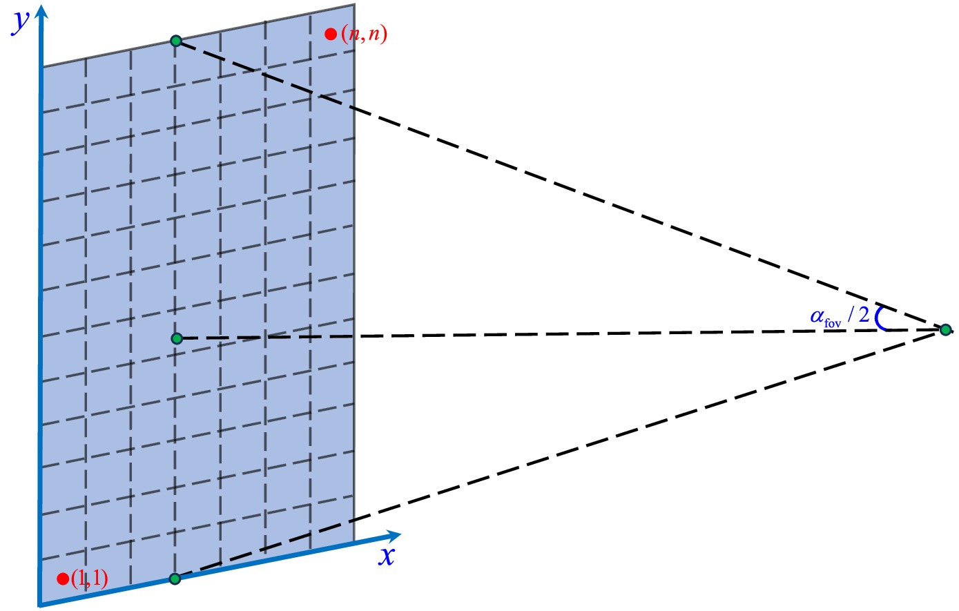
Figure 6. (color online) Fisheye camera field of view with
$ n \times n $ pixels, where the blue plane represents the imaging plane.In Fig. 7, we fix
$ \lambda = 0.1 $ and$ {\cal{G}} = 0.5 $ and study the effect of the rotation parameter a on the shadow image under the spherical light source model. The black region at the center of the figure represents the inner shadow, where photons pass through the equatorial plane zero times and directly fall into the event horizon, and hence, the corresponding image pixels are black. The white curve in the image represents the Einstein ring. Inside the Einstein ring, the D-shaped petals representing the celestial quadrants are divided by the gray curve, which represents the photon’s trajectory. Some photons fall into the event horizon, so these gray curves are not closed. When$ a \to 0 $ , the black hole shadow appears as a perfect circle, and the intersection of the blue and yellow regions is perpendicular to the horizontal axis. This indicates that the black hole behaves like a static black hole and does not produce a noticeable dragging effect on the background celestial sphere. As a increases, the vertical size of the shadow remains almost unchanged; however, it gradually shifts to the right in the horizontal direction, resulting in the shadow adapting a D-shape. This is similar to the change in the shadow of rotating black holes, such as the Kerr black hole. Simultaneously, the increase in a causes the black hole to exert a dragging effect on the celestial sphere. Particularly in Fig. 7(c), we can clearly observe that the yellow region on the left side of the black hole shadow overlaps with the green region. Interestingly, as a increases, the Einstein ring no longer maintains a complete circular shape and breaks at the top and bottom, forming multiple arc segments, due to the weakening of the gravitational lensed effect caused by the increase in a.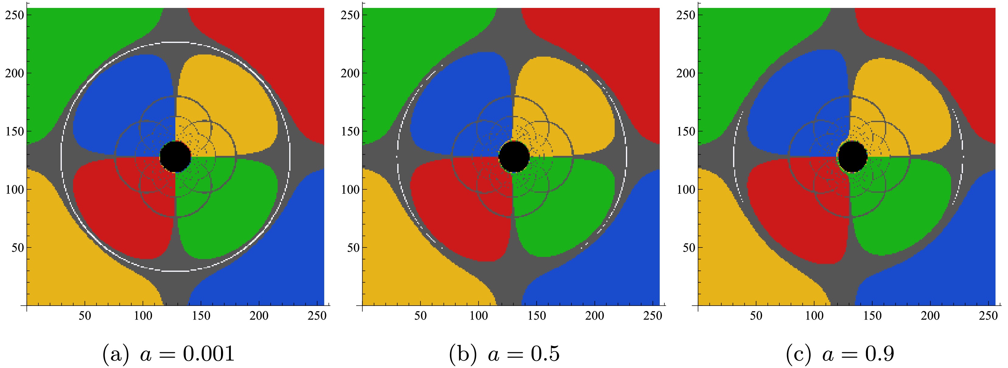
Figure 7. (color online) Impact of the rotation parameter a on the shadow image of a rotating black hole in KR gravity with a spherical light source. From left to right, the values of a are
$ 0.001 $ ,$ 0.5 $ , and$ 0.9 $ , with fixed parameters$ \lambda = 0.1 $ ,$ {\cal{G}} = 0.5 $ ,$ M = 1 $ , and$ \theta_o = 90^{\circ} $ .In Fig. 8, we fix
$ \lambda = 0.9 $ and$ a = 0.001 $ and study the effect of the spontaneous Lorentz symmetry violation parameter$ {\cal{G}} $ on the black hole shadow image. When$ a \to 0 $ , the black hole shadow appears as a perfect circle, with no noticeable dragging effect on the background celestial sphere. From left to right, as$ {\cal{G}} $ increases, although the Einstein ring and photon trajectories do not change significantly, the size of the shadow image decreases noticeably. In Fig. 9, we fix$ {\cal{G}} = a = 0.5 $ and study the effect of the spontaneous Lorentz symmetry violation parameter λ on the shadow image. In this case, the Einstein ring also breaks, but the photon trajectories inside the Einstein ring do not change significantly. Because$ a \neq 0 $ , the shadow image is no longer a perfect circle but an ellipse, and as λ increases, the shadow gradually shrinks. The above analysis shows that under the spherical light source model, the spontaneous Lorentz symmetry violation parameters λ and$ {\cal{G}} $ primarily affect the size of the shadow, while the rotation parameter a primarily affects the shape of the shadow. When$ a \neq 0 $ , the Einstein ring may break. This analysis helps differentiate rotating black holes in KR gravity from black holes in other spacetimes.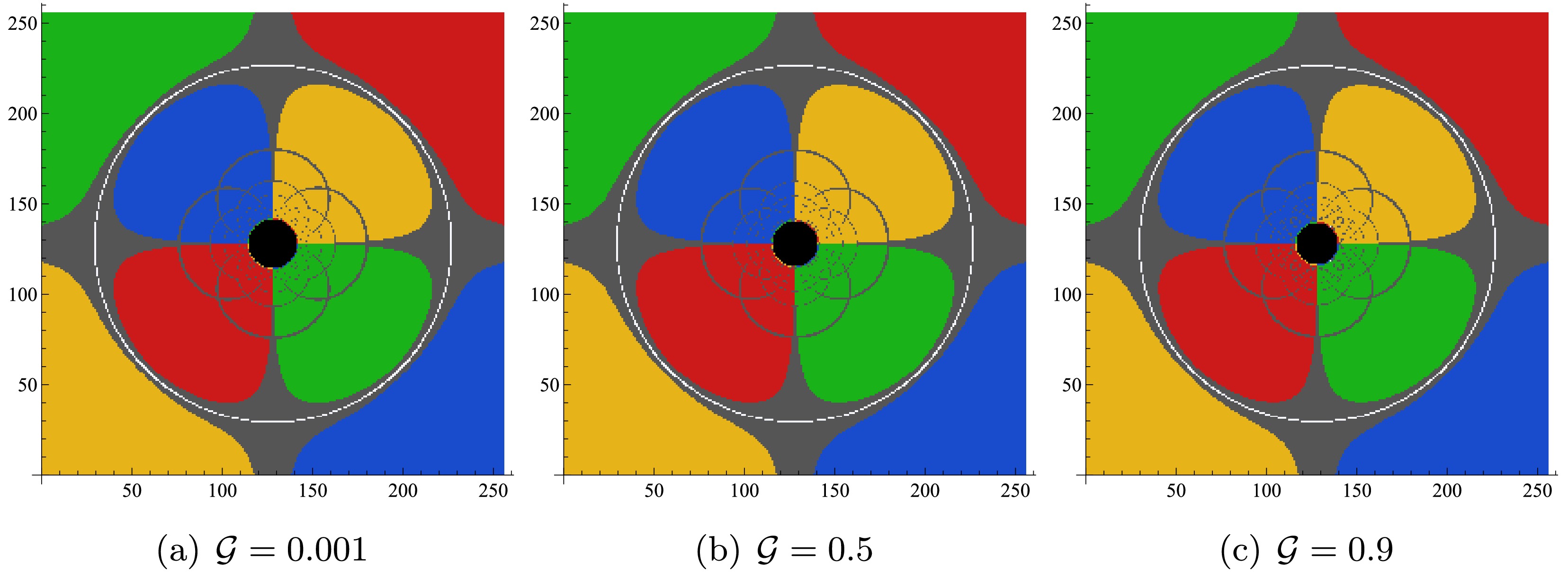
Figure 8. (color online) Impact of the spontaneous Lorentz symmetry violation parameter
$ {\cal{G}} $ on the shadow image of a rotating black hole in KR gravity with a spherical light source. From left to right, the values of$ {\cal{G}} $ are$ 0.001 $ ,$ 0.5 $ , and$ 0.9 $ , with fixed parameters$ \lambda = 0.9 $ ,$ a = 0.001 $ ,$ M = 1 $ , and$ \theta_o = 90^{\circ} $ .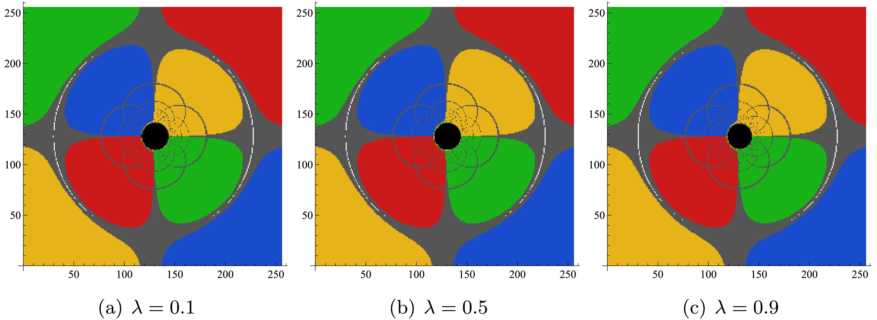
Figure 9. (color online) Impact of the spontaneous Lorentz symmetry violation parameter λ on the shadow image of a rotating black hole in KR gravity with a spherical light source. From left to right, the values of λ are
$ 0.1 $ ,$ 0.5 $ , and$ 0.9 $ , with fixed parameters$ {\cal{G}} = a = 0.5 $ ,$ M = 1 $ , and$ \theta_o = 90^{\circ} $ . -
In this section, we will use the backward ray-tracing techniques to discuss the shadow image of a black hole under the spherical light source model. In the spherical light source model, the black hole is located at the center of the celestial sphere, with the rotation axis pointing towards the north pole. The size of the black hole is significantly smaller than the diameter of the celestial sphere, and the observer is positioned on the celestial equator. For clarity, the celestial sphere is divided into four quadrants, labeled in red, blue, yellow, and green. A white reference light source is placed opposite the observer on the celestial sphere to study the strong gravitational lensed effect of the Einstein ring. The backward ray-tracing techniques assumes that the observer emits photons, and pixel mapping is performed by numerically solving the null geodesic equations. The advantage of this method is that it does not require considering photons that are emitted by the light source but do not reach the observer, thus simplifying the calculations. By using the backward ray-tracing techniques, once a photon reaches the celestial sphere, the corresponding pixel color is determined, with the photons that reach the event horizon marked in black.
To image the black hole shadow, we further discuss the camera projection. As mentioned earlier, we adopt the fisheye camera model, where the angle of field of view
$ \alpha_{\mathrm{fov}} $ determines the camera's viewing range. Let the Cartesian coordinates of the imaging plane be$ (x, y) $ . For convenience in calculation, we take$ \alpha_{\mathrm{fov}}/2 $ in both the x and y directions, thus defining a square screen with a side length of$ L = 2\left|\overrightarrow{OQ}\right|\tan\frac{\alpha_{\mathrm{fov}}}{2}. $
(45) The imaging plane is divided into
$ n \times n $ pixels, with the side length of each pixel being$ l = \frac{L}{n} = \frac{2}{n}\left|\overrightarrow{OQ}\right|\tan\frac{\alpha_{\mathrm{fov}}}{2}. $
(46) The center of each pixel is labeled by the coordinates
$ (i, j) $ , with the bottom-left pixel defined as$ (1, 1) $ and the top-right pixel defined as$ (n, n) $ , where i and j range from 1 to n (in this paper, we take$ n = 256 $ ). The relationship between$ (x_Q, y_Q) $ (see (38)) and the pixel coordinates$ (i, j) $ is given by$ x_Q = l\left(i - \frac{n+1}{2}\right),\quad y_Q = l\left(j - \frac{n+1}{2}\right). $
(47) By comparing Eqs. (38) and (47), we can see that the relationship between the pixel coordinates
$ (i, j) $ and the celestial coordinates$ (\Theta, \Phi) $ is$ \begin{aligned}[b]& \tan\frac{\Theta}{2} = \frac{1}{n}\tan\left(\frac{\alpha_{\mathrm{fov}}}{2}\right) \sqrt{\left(i - \frac{n+1}{2}\right)^2 + \left(j - \frac{n+1}{2}\right)^2}, \\ & \tan\Phi = \frac{2j - (n+1)}{2i - (n+1)}. \end{aligned} $
(48) Figure 6 shows a schematic of the fisheye camera. Using the above method, we can plot the black hole shadow image under the spherical light source model.
Figure 6. (color online) Fisheye camera field of view with
$ n \times n $ pixels, where the blue plane represents the imaging plane.In Fig. 7, we fix
$ \lambda = 0.1 $ and$ {\cal{G}} = 0.5 $ and study the effect of the rotation parameter a on the shadow image under the spherical light source model. The black region at the center of the figure represents the inner shadow, where photons pass through the equatorial plane zero times and directly fall into the event horizon, and hence, the corresponding image pixels are black. The white curve in the image represents the Einstein ring. Inside the Einstein ring, the D-shaped petals representing the celestial quadrants are divided by the gray curve, which represents the photon’s trajectory. Some photons fall into the event horizon, so these gray curves are not closed. When$ a \to 0 $ , the black hole shadow appears as a perfect circle, and the intersection of the blue and yellow regions is perpendicular to the horizontal axis. This indicates that the black hole behaves like a static black hole and does not produce a noticeable dragging effect on the background celestial sphere. As a increases, the vertical size of the shadow remains almost unchanged; however, it gradually shifts to the right in the horizontal direction, resulting in the shadow adapting a D-shape. This is similar to the change in the shadow of rotating black holes, such as the Kerr black hole. Simultaneously, the increase in a causes the black hole to exert a dragging effect on the celestial sphere. Particularly in Fig. 7(c), we can clearly observe that the yellow region on the left side of the black hole shadow overlaps with the green region. Interestingly, as a increases, the Einstein ring no longer maintains a complete circular shape and breaks at the top and bottom, forming multiple arc segments, due to the weakening of the gravitational lensed effect caused by the increase in a.
Figure 7. (color online) Impact of the rotation parameter a on the shadow image of a rotating black hole in KR gravity with a spherical light source. From left to right, the values of a are
$ 0.001 $ ,$ 0.5 $ , and$ 0.9 $ , with fixed parameters$ \lambda = 0.1 $ ,$ {\cal{G}} = 0.5 $ ,$ M = 1 $ , and$ \theta_o = 90^{\circ} $ .In Fig. 8, we fix
$ \lambda = 0.9 $ and$ a = 0.001 $ and study the effect of the spontaneous Lorentz symmetry violation parameter$ {\cal{G}} $ on the black hole shadow image. When$ a \to 0 $ , the black hole shadow appears as a perfect circle, with no noticeable dragging effect on the background celestial sphere. From left to right, as$ {\cal{G}} $ increases, although the Einstein ring and photon trajectories do not change significantly, the size of the shadow image decreases noticeably. In Fig. 9, we fix$ {\cal{G}} = a = 0.5 $ and study the effect of the spontaneous Lorentz symmetry violation parameter λ on the shadow image. In this case, the Einstein ring also breaks, but the photon trajectories inside the Einstein ring do not change significantly. Because$ a \neq 0 $ , the shadow image is no longer a perfect circle but an ellipse, and as λ increases, the shadow gradually shrinks. The above analysis shows that under the spherical light source model, the spontaneous Lorentz symmetry violation parameters λ and$ {\cal{G}} $ primarily affect the size of the shadow, while the rotation parameter a primarily affects the shape of the shadow. When$ a \neq 0 $ , the Einstein ring may break. This analysis helps differentiate rotating black holes in KR gravity from black holes in other spacetimes.
Figure 8. (color online) Impact of the spontaneous Lorentz symmetry violation parameter
$ {\cal{G}} $ on the shadow image of a rotating black hole in KR gravity with a spherical light source. From left to right, the values of$ {\cal{G}} $ are$ 0.001 $ ,$ 0.5 $ , and$ 0.9 $ , with fixed parameters$ \lambda = 0.9 $ ,$ a = 0.001 $ ,$ M = 1 $ , and$ \theta_o = 90^{\circ} $ .
Figure 9. (color online) Impact of the spontaneous Lorentz symmetry violation parameter λ on the shadow image of a rotating black hole in KR gravity with a spherical light source. From left to right, the values of λ are
$ 0.1 $ ,$ 0.5 $ , and$ 0.9 $ , with fixed parameters$ {\cal{G}} = a = 0.5 $ ,$ M = 1 $ , and$ \theta_o = 90^{\circ} $ . -
In this section, we will use the backward ray-tracing techniques to discuss the shadow image of a black hole under the spherical light source model. In the spherical light source model, the black hole is located at the center of the celestial sphere, with the rotation axis pointing towards the north pole. The size of the black hole is much smaller than the diameter of the celestial sphere, and the observer is positioned on the celestial equator. For clarity, the celestial sphere is divided into four quadrants, which are labeled in red, blue, yellow, and green. A white reference light source is placed opposite the observer on the celestial sphere to study the strong gravitational lensed effect of the Einstein ring. The backward ray-tracing techniques assumes that the observer emits photons, and pixel mapping is performed by numerically solving the null geodesic equations. The advantage of this method is that it does not require considering photons that are emitted by the light source but do not reach the observer, thus simplifying the calculations. By using the backward ray-tracing techniques, once a photon reaches the celestial sphere, the corresponding pixel color is determined, with the photons that reach the event horizon marked in black.
To image the black hole shadow, we further discuss the camera projection. As mentioned earlier, we adopt the fisheye camera model, where the angle of field of view
$ \alpha_{\mathrm{fov}} $ determines the camera's viewing range. Let the Cartesian coordinates of the imaging plane be$ (x, y) $ . For convenience in calculation, we take$ \alpha_{\mathrm{fov}}/2 $ in both the x and y directions, thus defining a square screen with a side length of$ L = 2\left|\overrightarrow{OQ}\right|\tan\frac{\alpha_{\mathrm{fov}}}{2}. $

(45) The imaging plane is divided into
$ n \times n $ pixels, with the side length of each pixel being$ l = \frac{L}{n} = \frac{2}{n}\left|\overrightarrow{OQ}\right|\tan\frac{\alpha_{\mathrm{fov}}}{2}. $

(46) The center of each pixel is labeled by the coordinates
$ (i, j) $ , with the bottom-left pixel defined as$ (1, 1) $ and the top-right pixel defined as$ (n, n) $ , where i and j range from 1 to n (in this paper, we take$ n = 256 $ ). The relationship between$ (x_Q, y_Q) $ (see (38)) and the pixel coordinates$ (i, j) $ is given by$ x_Q = l\left(i - \frac{n+1}{2}\right),\quad y_Q = l\left(j - \frac{n+1}{2}\right). $

(47) By comparing equation (38) and equation (47), we can see that the relationship between the pixel coordinates
$ (i, j) $ and the celestial coordinates$ (\Theta, \Phi) $ is$ \begin{aligned}[b]& \tan\frac{\Theta}{2} = \frac{1}{n}\tan\left(\frac{\alpha_{\mathrm{fov}}}{2}\right) \sqrt{\left(i - \frac{n+1}{2}\right)^2 + \left(j - \frac{n+1}{2}\right)^2}, \\ & \tan\Phi = \frac{2j - (n+1)}{2i - (n+1)}. \end{aligned} $

(48) Figure 6 shows a schematic of the fisheye camera. Using the above method, we can plot the black hole shadow image under the spherical light source model.
Figure 6. (color online) Fisheye camera field of view with
$ n \times n $ pixels, where the blue plane represents the imaging plane.In Figure 7, we fix
$ \lambda = 0.1 $ and$ {\cal{G}} = 0.5 $ and study the effect of the rotation parameter a on the shadow image under the spherical light source model. The black region at the center of the figure represents the inner shadow, where photons pass through the equatorial plane zero times and directly fall into the event horizon, so the corresponding image pixels are black. The white curve in the image represents the Einstein ring. Inside the Einstein ring, the D-shaped petals representing the celestial quadrants are divided by the gray curve, which represents the photon’s trajectory. Some photons fall into the event horizon, so these gray curves are not closed. When$ a \to 0 $ , the black hole shadow appears as a perfect circle, and the intersection of the blue and yellow regions inside the Einstein ring is perpendicular to the horizontal axis, indicating that the black hole behaves like a static black hole and does not produce a noticeable dragging effect on the background celestial sphere. As a increases, the vertical size of the shadow remains almost unchanged, but it gradually shifts to the right in the horizontal direction, causing the shadow to take on a D-shaped. This trend is similar to the change in the shadow of rotating black holes, such as the Kerr black hole. At the same time, the increase in a causes the black hole to exert a dragging effect on the celestial sphere. Particularly in Figure 7(c), we can clearly observe that the yellow region on the left side of the black hole shadow overlaps with the green region. Interestingly, as a increases, the Einstein ring no longer maintains a complete circular shape and breaks at the top and bottom, forming multiple arc segments. This may be due to the weakening of the gravitational lensed effect caused by the increase in a.
Figure 7. (color online) The impact of the rotation parameter a on the shadow image of a rotating black hole in KR gravity with a spherical light source. From left to right, the values of a are
$ 0.001 $ ,$ 0.5 $ , and$ 0.9 $ , with fixed parameters$ \lambda = 0.1 $ ,$ {\cal{G}} = 0.5 $ ,$ M = 1 $ , and$ \theta_o = 90^{\circ} $ .In Figure 8, we fix
$ \lambda = 0.9 $ and$ a = 0.001 $ and study the effect of the spontaneous Lorentz symmetry violation parameter$ {\cal{G}} $ on the black hole shadow image. When$ a \to 0 $ , the black hole shadow appears as a perfect circle, with no noticeable dragging effect on the background celestial sphere. From left to right, as$ {\cal{G}} $ increases, although the Einstein ring and photon trajectories do not change significantly, the size of the shadow image decreases noticeably. In Figure 9, we fix$ {\cal{G}} = a = 0.5 $ and study the effect of the spontaneous Lorentz symmetry violation parameter λ on the shadow image. In this case, the Einstein ring also breaks, but the photon trajectories inside the Einstein ring do not change significantly. Since$ a \neq 0 $ , the shadow image is no longer a perfect circle but an ellipse, and as λ increases, the shadow gradually shrinks. The above analysis shows that under the spherical light source model, the spontaneous Lorentz symmetry violation parameters λ and$ {\cal{G}} $ primarily affect the size of the shadow, while the rotation parameter a primarily affects the shape of the shadow. When$ a \neq 0 $ , the Einstein ring may break. This analysis helps differentiate rotating black holes in KR gravity from black holes in other spacetimes.
Figure 8. (color online) The impact of the spontaneous Lorentz symmetry violation parameter
$ {\cal{G}} $ on the shadow image of a rotating black hole in KR gravity with a spherical light source. From left to right, the values of$ {\cal{G}} $ are$ 0.001 $ ,$ 0.5 $ , and$ 0.9 $ , with fixed parameters$ \lambda = 0.9 $ ,$ a = 0.001 $ ,$ M = 1 $ , and$ \theta_o = 90^{\circ} $ .
Figure 9. (color online) The impact of the spontaneous Lorentz symmetry violation parameter λ on the shadow image of a rotating black hole in KR gravity with a spherical light source. From left to right, the values of λ are
$ 0.1 $ ,$ 0.5 $ , and$ 0.9 $ , with fixed parameters$ {\cal{G}} = a = 0.5 $ ,$ M = 1 $ , and$ \theta_o = 90^{\circ} $ . -
Previously, we discussed the black hole shadow image under the spherical light source model. In reality, an accretion disk exists around the black hole; therefore, studying the black hole shadow image illuminated by the accretion disk as a light source is of greater significance. For simplicity, we assume the accretion disk is optically and geometrically thin and located in the equatorial plane, with the observer sufficiently far away, i.e.,
$ \theta_o = \pi/2, r_o \gg M = 1 $ . The accretion disk comprises free electrically neutral plasma moving along timelike geodesics in the equatorial plane. Matter that is accreted by the black hole will fall into the event horizon if it is too close to the black hole; if it is far, it may orbit the black hole along a stable orbit. To better describe this phenomenon, we introduce the concept of the innermost stable circular orbit (ISCO), which is located at the inner edge of the accretion disk and is the last region where matter can safely orbit without falling into the event horizon. The accretion disk is divided into two regions by the ISCO: inside the ISCO, the accreting material falls into the event horizon along plunging orbits, whereas outside the ISCO, the accretion disk material orbits the black hole along a Keplerian orbit. Conversely, according to the reference [44], light rays may interact with the accretion disk multiple times, with each interaction increasing the brightness of the black hole shadow image. We denote the position where the photon interacts with the accretion disk for the nth time as$ r_n $ ($ n = 1, 2, 3, \dots $ ). When$ n = 1 $ , the resulting image is called the direct image; when$ n = 2 $ , it is called the lensed image; when$ n>2 $ , it is called the higher-order images. Because direct and lensed images contribute over 95% to the total luminosity, we paper mainly focus on the cases of$ n = 1 $ and$ n = 2 $ , i.e., direct and lensed images. Notably, regardless of changes in reflection effects or the thickness of the accretion disk, the above phenomena always occur. In Fig. 10, we show a schematic of the black hole imaging with the thin accretion disk as the light source.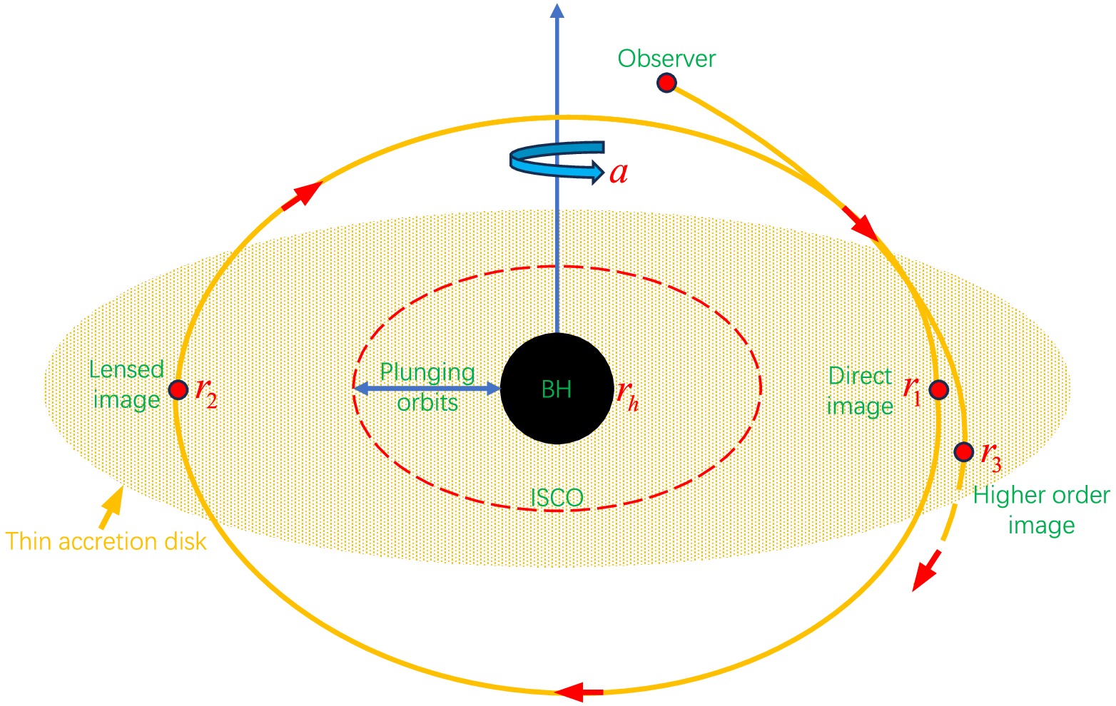
Figure 10. (color online) Imaging the black hole with a thin accretion disks. The black sphere represents the black hole, the red dashed line represents the ISCO, the orange curve represents the trajectory of photons emitted by the observer in the backward ray-tracing techniques, and the orange elliptical disk represents the thin accretion disk.
Inside the event horizon, matter falls into the black hole, so in this paper, we assume the accretion disk extends inward to the black hole’s event horizon
$ r_h $ and outward to a sufficiently distant point, denoted as$ r_f $ . The observer’s position$ r_o $ satisfies$ r_h \ll r_o < r_f $ . To obtain the black hole shadow image under the thin accretion disk model, we first need to determine the position of the ISCO. The position of the ISCO is typically determined by the following conditions$ {\cal{V}}_{\rm eff}\bigg|_{r = r_{I}} = 0, $
(49) $ \frac{\partial {\cal{V}}_{\rm eff}}{\partial r}\bigg|_{r = r_{I}} = 0, $
(50) $ \frac{\partial^2 {\cal{V}}_{\rm eff}}{\partial r^2}\bigg|_{r = r_{I}} = 0, $
(51) where
$ r_{I} $ is the position of the ISCO, and$ {\cal{V}}_{\rm eff} $ is a function of the radial distance r that represents the effective potential of a massive electrically neutral particle. It can be expressed as$ {\cal{V}}_{\rm eff}(r,\tilde{{\cal{E}}},\tilde{{\cal{L}}}) = (1+g^{tt}\tilde{{\cal{E}}}^2+g^{\phi\phi}\tilde{{\cal{L}}}^2-2g^{t\phi}\tilde{{\cal{E}}}\tilde{{\cal{L}}})\big|_{\theta = \pi/2}, $
(52) where
$ \tilde{{\cal{E}}} = -\frac{g_{tt}+g_{t\phi}\bar{\omega}}{\sqrt{-g_{tt}-2g_{t\phi}\bar{\omega}-g_{\phi\phi}\bar{\omega}^2}}, $
(53) $ \tilde{{\cal{L}}} = \frac{g_{t\phi}+g_{\phi\phi}\bar{\omega}}{\sqrt{-g_{tt}-2g_{t\phi}\bar{\omega}-g_{\phi\phi}\bar{\omega}^2}}, $
(54) representing the specific energy and specific angular momentum of the massive electrically neutral particle, provided by the Killing vector field. The angular velocity
$ \bar{\omega} $ is defined as$ \bar{\omega} = \frac{{\rm d}\phi}{{\rm d}t}\equiv\frac{\dfrac{\partial g_{t\phi}}{\partial r}+\sqrt{\dfrac{\partial^2 g_{t\phi}}{\partial r^2}-\dfrac{\partial g_{tt}}{\partial r}\dfrac{\partial g_{\phi\phi}}{\partial r}}}{\dfrac{\partial g_{\phi\phi}}{\partial r}}. $
(55) At
$ r = r_{I} $ ,$ \tilde{{\cal{E}}}_{I} $ and$ \tilde{{\cal{L}}}_{I} $ are conserved quantities; when$ r>r_{I} $ , the matter in the accretion disk moves along a Keplerian orbit, and its four-velocity is$ U_{\rm out}^{a} = \sqrt{\frac{1}{-g_{tt}-2g_{t\phi}\bar{\omega}-g_{\phi\phi}\bar{\omega}^2}}\left(1,0,0,\bar{\omega}\right)\bigg|_{\theta = \pi/2}. $
(56) When
$ r<r_{I} $ , the accreting material freely falls from$ r_{I} $ toward the black hole's event horizon. For simplicity, we assume that$ \tilde{{\cal{E}}}_{I} $ and$ \tilde{{\cal{L}}}_{I} $ remain constant at$ r_{I} $ . In this case, the four-velocity of the freely falling material is given by$ \begin{aligned}[b]& U_{\rm in}^{t} = \left(-g^{tt}\tilde{{\cal{E}}}_{I}+g^{t\phi}\tilde{{\cal{L}}}_{I}\right)\bigg|_{\theta = \pi/2}, \\ & U_{\rm in}^{r} = -\sqrt{-\frac{g_{tt}U_{\rm in}^{t}U_{\rm in}^{t}+2g_{t\phi}U_{\rm in}^{t}U_{\rm in}^{\phi}+g_{\phi\phi}U_{\rm in}^{\phi}U_{\rm in}^{\phi}+1}{g_{rr}}}\bigg|_{\theta = \pi/2}, \\ & U_{\rm in}^{\theta} = 0, \\ & U_{\rm in}^{\phi} = \left(-g^{t\phi}\tilde{{\cal{E}}}_{I}+g^{\phi\phi}\tilde{{\cal{L}}}_{I}\right)\bigg|_{\theta = \pi/2}. \end{aligned} $
(57) In these expressions, the negative sign in front of
$ U_{\rm in}^{r} $ indicates that the particle moves toward the black hole event horizon, and the radial distance r lies within the range$ r_{h} < r < r_{I} $ .When using the backward ray-tracing techniques at the observer's location, photons may interact multiple times with the accretion disk in the equatorial plane, and each interaction increases the luminosity of the black hole shadow image. In general, when a photon interacts with the accretion disk, the intensity changes due to the emission and absorption of the photon. To simplify the model, we ignore the reflection effects in this study. Under the above assumptions, the change in intensity is described by
$ \frac{\rm d}{{\rm d}\tau}\left(\frac{{\cal{S}}_\nu}{\nu^3}\right) = \frac{{\cal{E}}_\nu-{\cal{A}}_\nu {\cal{S}}_\nu}{\nu^2}, $
(58) where τ is the affine parameter of the photon geodesic.
$ {\cal{S}}_{\nu} $ ,$ {\cal{E}}_{\nu} $ , and$ {\cal{A}}_{\nu} $ represent the specific intensity, emissivity, and absorption coefficient at the frequency ν, respectively. When no absorption or emission occurs,$ {\cal{S}}_{\nu}/\nu^3 $ remains constant along the geodesic. In the thin disk approximation, the accretion disk is located in the equatorial plane; therefore, outside the equatorial plane,$ {\cal{E}}_\nu = {\cal{A}}_\nu = 0 $ . In this case, the total intensity at each position on the observation screen is given by$ {\cal{I}}_{o} = \sum\limits_{n = 1}^{N_{\max}} f_n(\chi_n)^3 {\cal{E}}_n, $
(59) where
$ n = 1,\ldots,N_{\max} $ represents the number of times the photon crosses the equatorial plane,$ f_n $ is the fudge factor, which needs to be determined according to the specific accretion disk model (here,$ f_n = 1 $ is set), and$ \chi_n\equiv\nu_0/\nu_n $ is the redshift factor, where$ \nu_0 $ is the frequency measured on the observer's screen, and$ \nu_n $ is the frequency measured in the local rest frames comoving with the accretion disk. Considering the wavelength of the black hole image observed by EHT is$ 1.3 \ \mathrm{mm} \,(230 \ \mathrm{GHz}) $ , the emissivity of the thin disk,$ {\cal{E}}_{\nu} $ , is treated as a second-order polynomial in log-space and is given by$ {\cal{E}}_{\nu}(r) = \exp\left(-\frac12k^2-2k\right),\quad k = \log\frac r{r_h}. $
(60) Because the accretion disk comprises electrically neutral plasma, it moves along a timelike geodesic with
$ \tilde{{\cal{E}}} $ and$ \tilde{{\cal{L}}} $ . When$ r>r_{I} $ , the redshift factor is given by$ \chi_n^{out} = \frac{\alpha\left(1-\gamma\dfrac{p_\phi}{p_t}\right)}{\beta\left(1+\bar{\omega}\dfrac{p_\phi}{p_t}\right)}\Bigg|_{r = r_n},\quad r>r_{I}, $
(61) where
$ \gamma = \frac{g_{t\phi}}{g_{\phi\phi}}, $
(62) $ \alpha = \sqrt{\frac{-g_{\phi\phi}}{g_{tt}g_{\phi\phi}-g_{t\phi}^{2}}}, $
(63) $ \beta = \sqrt{\frac{-1}{g_{tt}+2g_{t\phi}\bar{\omega}+g_{\phi\phi}\bar{\omega}^{2}}}, $
(64) where
$ \bar{\omega} $ is calculated using Eq. (55). The ratio of the energy measured on the observer's screen to the energy along a null geodesic is$ z = \alpha\left(1-\gamma\frac{p_{\phi}}{p_{t}}\right). $
(65) For asymptotically flat spacetime, when the observer is at infinity,
$ z = 1 $ . When$ r<r_{I} $ , the accreting material falls freely from$ r_{I} $ toward the black hole event horizon along a plunging orbit with$ \tilde{{\cal{E}}} $ and$ \tilde{{\cal{L}}} $ . The radial velocity is$ U_{\rm in}^{r} $ , and at this point, the redshift factor is given by$\begin{aligned}[b]& \chi_{n}^{\rm in} = \frac1{U_{\rm in}^rp_r/p_t-\tilde{{\cal{E}}}_{I}(g^{tt}-g^{t\phi}p_\phi/p_t)+\tilde{{\cal{L}}}_{I}(g^{\phi\phi}p_\phi/p_t+g^{t\phi})}\Bigg|_{r = r_n},\\& r<r_{I}. \end{aligned}$
(66) With the above discussion, we can choose an appropriate color-function to plot the black hole shadow image with a thin accretion disk as the light source.
-
Previously, we discussed the black hole shadow image under the spherical light source model. In reality, an accretion disk exists around the black hole; therefore, studying the black hole shadow image illuminated by the accretion disk as a light source is of greater significance. For simplicity, we assume the accretion disk is optically and geometrically thin and located in the equatorial plane, with the observer sufficiently far away, i.e.,
$ \theta_o = \pi/2, r_o \gg M = 1 $ . The accretion disk comprises free electrically neutral plasma moving along timelike geodesics in the equatorial plane. Matter that is accreted by the black hole will fall into the event horizon if it is too close to the black hole; if it is far, it may orbit the black hole along a stable orbit. To better describe this phenomenon, we introduce the concept of the innermost stable circular orbit (ISCO), which is located at the inner edge of the accretion disk and is the last region where matter can safely orbit without falling into the event horizon. The accretion disk is divided into two regions by the ISCO: inside the ISCO, the accreting material falls into the event horizon along plunging orbits, whereas outside the ISCO, the accretion disk material orbits the black hole along a Keplerian orbit. Conversely, according to the reference [44], light rays may interact with the accretion disk multiple times, with each interaction increasing the brightness of the black hole shadow image. We denote the position where the photon interacts with the accretion disk for the nth time as$ r_n $ ($ n = 1, 2, 3, \dots $ ). When$ n = 1 $ , the resulting image is called the direct image; when$ n = 2 $ , it is called the lensed image; when$ n>2 $ , it is called the higher-order images. Because direct and lensed images contribute over 95% to the total luminosity, we paper mainly focus on the cases of$ n = 1 $ and$ n = 2 $ , i.e., direct and lensed images. Notably, regardless of changes in reflection effects or the thickness of the accretion disk, the above phenomena always occur. In Fig. 10, we show a schematic of the black hole imaging with the thin accretion disk as the light source.
Figure 10. (color online) Imaging the black hole with a thin accretion disks. The black sphere represents the black hole, the red dashed line represents the ISCO, the orange curve represents the trajectory of photons emitted by the observer in the backward ray-tracing techniques, and the orange elliptical disk represents the thin accretion disk.
Inside the event horizon, matter falls into the black hole, so in this paper, we assume the accretion disk extends inward to the black hole’s event horizon
$ r_h $ and outward to a sufficiently distant point, denoted as$ r_f $ . The observer’s position$ r_o $ satisfies$ r_h \ll r_o \lt r_f $ . To obtain the black hole shadow image under the thin accretion disk model, we first need to determine the position of the ISCO. The position of the ISCO is typically determined by the following conditions$ {\cal{V}}_{\rm eff}\bigg|_{r = r_{I}} = 0, $
(49) $ \frac{\partial {\cal{V}}_{\rm eff}}{\partial r}\bigg|_{r = r_{I}} = 0, $
(50) $ \frac{\partial^2 {\cal{V}}_{\rm eff}}{\partial r^2}\bigg|_{r = r_{I}} = 0, $
(51) where
$ r_{I} $ is the position of the ISCO, and$ {\cal{V}}_{\rm eff} $ is a function of the radial distance r that represents the effective potential of a massive electrically neutral particle. It can be expressed as$ {\cal{V}}_{\rm eff}(r,\tilde{{\cal{E}}},\tilde{{\cal{L}}}) = (1+g^{tt}\tilde{{\cal{E}}}^2+g^{\phi\phi}\tilde{{\cal{L}}}^2-2g^{t\phi}\tilde{{\cal{E}}}\tilde{{\cal{L}}})\big|_{\theta = \pi/2}, $
(52) where
$ \tilde{{\cal{E}}} = -\frac{g_{tt}+g_{t\phi}\bar{\omega}}{\sqrt{-g_{tt}-2g_{t\phi}\bar{\omega}-g_{\phi\phi}\bar{\omega}^2}}, $
(53) $ \tilde{{\cal{L}}} = \frac{g_{t\phi}+g_{\phi\phi}\bar{\omega}}{\sqrt{-g_{tt}-2g_{t\phi}\bar{\omega}-g_{\phi\phi}\bar{\omega}^2}}, $
(54) representing the specific energy and specific angular momentum of the massive electrically neutral particle, provided by the Killing vector field. The angular velocity
$ \bar{\omega} $ is defined as$ \bar{\omega} = \frac{{\rm d}\phi}{{\rm d}t}\equiv\frac{\dfrac{\partial g_{t\phi}}{\partial r}+\sqrt{\dfrac{\partial^2 g_{t\phi}}{\partial r^2}-\dfrac{\partial g_{tt}}{\partial r}\dfrac{\partial g_{\phi\phi}}{\partial r}}}{\dfrac{\partial g_{\phi\phi}}{\partial r}}. $
(55) At
$ r = r_{I} $ ,$ \tilde{{\cal{E}}}_{I} $ and$ \tilde{{\cal{L}}}_{I} $ are conserved quantities; when$ r>r_{I} $ , the matter in the accretion disk moves along a Keplerian orbit, and its four-velocity is$ U_{\rm out}^{a} = \sqrt{\frac{1}{-g_{tt}-2g_{t\phi}\bar{\omega}-g_{\phi\phi}\bar{\omega}^2}}\left(1,0,0,\bar{\omega}\right)\bigg|_{\theta = \pi/2}. $
(56) When
$ r<r_{I} $ , the accreting material freely falls from$ r_{I} $ toward the black hole's event horizon. For simplicity, we assume that$ \tilde{{\cal{E}}}_{I} $ and$ \tilde{{\cal{L}}}_{I} $ remain constant at$ r_{I} $ . In this case, the four-velocity of the freely falling material is given by$ \begin{aligned}[b]& U_{\rm in}^{t} = \left(-g^{tt}\tilde{{\cal{E}}}_{I}+g^{t\phi}\tilde{{\cal{L}}}_{I}\right)\bigg|_{\theta = \pi/2}, \\ & U_{\rm in}^{r} = -\sqrt{-\frac{g_{tt}U_{\rm in}^{t}U_{\rm in}^{t}+2g_{t\phi}U_{\rm in}^{t}U_{\rm in}^{\phi}+g_{\phi\phi}U_{\rm in}^{\phi}U_{\rm in}^{\phi}+1}{g_{rr}}}\bigg|_{\theta = \pi/2}, \\ & U_{\rm in}^{\theta} = 0, \\ & U_{\rm in}^{\phi} = \left(-g^{t\phi}\tilde{{\cal{E}}}_{I}+g^{\phi\phi}\tilde{{\cal{L}}}_{I}\right)\bigg|_{\theta = \pi/2}. \end{aligned} $
(57) In these expressions, the negative sign in front of
$ U_{\rm in}^{r} $ indicates that the particle moves toward the black hole event horizon, and the radial distance r lies within the range$ r_{h} \lt r \lt r_{I} $ .When using the backward ray-tracing techniques at the observer's location, photons may interact multiple times with the accretion disk in the equatorial plane, and each interaction increases the luminosity of the black hole shadow image. In general, when a photon interacts with the accretion disk, the intensity changes due to the emission and absorption of the photon. To simplify the model, we ignore the reflection effects in this study. Under the above assumptions, the change in intensity is described by
$ \frac{\rm d}{{\rm d}\tau}\left(\frac{{\cal{S}}_\nu}{\nu^3}\right) = \frac{{\cal{E}}_\nu-{\cal{A}}_\nu {\cal{S}}_\nu}{\nu^2}, $
(58) where τ is the affine parameter of the photon geodesic.
$ {\cal{S}}_{\nu} $ ,$ {\cal{E}}_{\nu} $ , and$ {\cal{A}}_{\nu} $ represent the specific intensity, emissivity, and absorption coefficient at the frequency ν, respectively. When no absorption or emission occurs,$ {\cal{S}}_{\nu}/\nu^3 $ remains constant along the geodesic. In the thin disk approximation, the accretion disk is located in the equatorial plane; therefore, outside the equatorial plane,$ {\cal{E}}_\nu = {\cal{A}}_\nu = 0 $ . In this case, the total intensity at each position on the observation screen is given by$ {\cal{I}}_{o} = \sum\limits_{n = 1}^{N_{\max}} f_n(\chi_n)^3 {\cal{E}}_n, $
(59) where
$ n = 1,\ldots,N_{\max} $ represents the number of times the photon crosses the equatorial plane,$ f_n $ is the fudge factor, which needs to be determined according to the specific accretion disk model (here,$ f_n = 1 $ is set), and$ \chi_n\equiv\nu_0/\nu_n $ is the redshift factor, where$ \nu_0 $ is the frequency measured on the observer's screen, and$ \nu_n $ is the frequency measured in the local rest frames comoving with the accretion disk. Considering the wavelength of the black hole image observed by EHT is$ 1.3 \ \mathrm{mm} \,(230 \ \mathrm{GHz}) $ , the emissivity of the thin disk,$ {\cal{E}}_{\nu} $ , is treated as a second-order polynomial in log-space and is given by$ {\cal{E}}_{\nu}(r) = \exp\left(-\frac12k^2-2k\right),\quad k = \log\frac r{r_h}. $
(60) Because the accretion disk comprises electrically neutral plasma, it moves along a timelike geodesic with
$ \tilde{{\cal{E}}} $ and$ \tilde{{\cal{L}}} $ . When$ r>r_{I} $ , the redshift factor is given by$ \chi_n^{out} = \frac{\alpha\left(1-\gamma\dfrac{p_\phi}{p_t}\right)}{\beta\left(1+\bar{\omega}\dfrac{p_\phi}{p_t}\right)}\Bigg|_{r = r_n},\quad r>r_{I}, $
(61) where
$ \gamma = \frac{g_{t\phi}}{g_{\phi\phi}}, $
(62) $ \alpha = \sqrt{\frac{-g_{\phi\phi}}{g_{tt}g_{\phi\phi}-g_{t\phi}^{2}}}, $
(63) $ \beta = \sqrt{\frac{-1}{g_{tt}+2g_{t\phi}\bar{\omega}+g_{\phi\phi}\bar{\omega}^{2}}}, $
(64) where
$ \bar{\omega} $ is calculated using Eq. (55). The ratio of the energy measured on the observer's screen to the energy along a null geodesic is$ z = \alpha\left(1-\gamma\frac{p_{\phi}}{p_{t}}\right). $
(65) For asymptotically flat spacetime, when the observer is at infinity,
$ z = 1 $ . When$ r<r_{I} $ , the accreting material falls freely from$ r_{I} $ toward the black hole event horizon along a plunging orbit with$ \tilde{{\cal{E}}} $ and$ \tilde{{\cal{L}}} $ . The radial velocity is$ U_{\rm in}^{r} $ , and at this point, the redshift factor is given by$\begin{aligned}[b]& \chi_{n}^{\rm in} = \frac1{U_{\rm in}^rp_r/p_t-\tilde{{\cal{E}}}_{I}(g^{tt}-g^{t\phi}p_\phi/p_t)+\tilde{{\cal{L}}}_{I}(g^{\phi\phi}p_\phi/p_t+g^{t\phi})}\Bigg|_{r = r_n},\\& r<r_{I}. \end{aligned}$
(66) With the above discussion, we can choose an appropriate color-function to plot the black hole shadow image with a thin accretion disk as the light source.
-
In the previous section, we discussed the black hole shadow image under the spherical light source model. However, in reality, there is an accretion disk around the black hole, so studying the black hole shadow image illuminated by the accretion disk as a light source is of greater significance. For simplicity, we assume the accretion disk is optically and geometrically thin and located in the equatorial plane, with the observer sufficiently far away, i.e.,
$ \theta_o = \pi/2, r_o \gg M = 1 $ . The accretion disk consists of free electrically neutral plasma moving along timelike geodesics in the equatorial plane. Matter that is accreted by the black hole will fall into the event horizon if it is too close to the black hole; if it is far enough, it may orbit the black hole along a stable orbit. To more intuitively describe this phenomenon, we introduce the concept of the innermost stable circular orbit (ISCO). The ISCO is located at the inner edge of the accretion disk and is the last region where matter can safely orbit without falling into the event horizon. The accretion disk is divided into two regions by the ISCO: inside the ISCO, the accreting material falls into the event horizon along plunging orbits, while outside the ISCO, the accretion disk material orbits the black hole along a Keplerian orbit. On the other hand, according to the reference [44], light rays may interact with the accretion disk multiple times, with each interaction increasing the brightness of the black hole shadow image. We denote the position where the photon interacts with the accretion disk for the nth time as$ r_n $ ($ n = 1, 2, 3, \dots $ ). When$ n = 1 $ , the resulting image is called the direct image; when$ n = 2 $ , it is called the lensed image; when$ n>2 $ , it is called the higher-order images. Since direct and lensed images contribute more than 95% to the total luminosity, this paper mainly focuses on the cases of$ n = 1 $ and$ n = 2 $ , i.e., direct and lensed images. It is worth noting that regardless of changes in reflection effects or the thickness of the accretion disk, the above phenomena always occur. In Figure 10, we show a schematic of the black hole imaging with the thin accretion disk as the light source.
Figure 10. (color online) Imaging the black hole with a thin accretion disks. The black sphere represents the black hole, the red dashed line represents the ISCO, the orange curve represents the trajectory of photons emitted by the observer in the backward ray-tracing techniques, and the orange elliptical disk represents the thin accretion disk.
Inside the event horizon, matter falls into the black hole, so in this paper, we assume the accretion disk extends inward to the black hole’s event horizon
$ r_h $ and outward to a sufficiently distant point, denoted as$ r_f $ . The observer’s position$ r_o $ satisfies$ r_h \ll r_o < r_f $ . To obtain the black hole shadow image under the thin accretion disk model, we first need to determine the position of the ISCO. The position of the ISCO is typically determined by the following conditions$ {\cal{V}}_{eff}\bigg|_{r = r_{I}} = 0, $

(49) $ \frac{\partial {\cal{V}}_{eff}}{\partial r}\bigg|_{r = r_{I}} = 0, $

(50) $ \frac{\partial^2 {\cal{V}}_{eff}}{\partial r^2}\bigg|_{r = r_{I}} = 0, $

(51) where
$ r_{I} $ is the position of the ISCO, and$ {\cal{V}}_{eff} $ is a function of the radial distance r that represents the effective potential of a massive electrically neutral particle. It can be expressed as$ {\cal{V}}_{eff}(r,\tilde{{\cal{E}}},\tilde{{\cal{L}}}) = (1+g^{tt}\tilde{{\cal{E}}}^2+g^{\phi\phi}\tilde{{\cal{L}}}^2-2g^{t\phi}\tilde{{\cal{E}}}\tilde{{\cal{L}}})\big|_{\theta = \pi/2}, $

(52) where
$ \tilde{{\cal{E}}} = -\frac{g_{tt}+g_{t\phi}\bar{\omega}}{\sqrt{-g_{tt}-2g_{t\phi}\bar{\omega}-g_{\phi\phi}\bar{\omega}^2}}, $

(53) $ \tilde{{\cal{L}}} = \frac{g_{t\phi}+g_{\phi\phi}\bar{\omega}}{\sqrt{-g_{tt}-2g_{t\phi}\bar{\omega}-g_{\phi\phi}\bar{\omega}^2}}, $

(54) representing the specific energy and specific angular momentum of the massive electrically neutral particle, provided by the Killing vector field. The angular velocity
$ \bar{\omega} $ is defined as$ \bar{\omega} = \frac{d\phi}{dt}\equiv\frac{\dfrac{\partial g_{t\phi}}{\partial r}+\sqrt{\dfrac{\partial^2 g_{t\phi}}{\partial r^2}-\dfrac{\partial g_{tt}}{\partial r}\dfrac{\partial g_{\phi\phi}}{\partial r}}}{\dfrac{\partial g_{\phi\phi}}{\partial r}}. $

(55) At
$ r = r_{I} $ ,$ \tilde{{\cal{E}}}_{I} $ and$ \tilde{{\cal{L}}}_{I} $ are conserved quantities; when$ r>r_{I} $ , the matter in the accretion disk moves along a Keplerian orbit, and its four-velocity is$ U_{out}^{a} = \sqrt{\frac{1}{-g_{tt}-2g_{t\phi}\bar{\omega}-g_{\phi\phi}\bar{\omega}^2}}\left(1,0,0,\bar{\omega}\right)\bigg|_{\theta = \pi/2}. $

(56) When
$ r<r_{I} $ , the accreting material freely falls from$ r_{I} $ toward the black hole's event horizon. For simplicity, we assume that$ \tilde{{\cal{E}}}_{I} $ and$ \tilde{{\cal{L}}}_{I} $ remain constant at$ r_{I} $ . In this case, the four-velocity of the freely falling material is given by$ \begin{aligned}[b]& U_{in}^{t} = \left(-g^{tt}\tilde{{\cal{E}}}_{I}+g^{t\phi}\tilde{{\cal{L}}}_{I}\right)\bigg|_{\theta = \pi/2}, \\ & U_{in}^{r} = -\sqrt{-\frac{g_{tt}U_{in}^{t}U_{in}^{t}+2g_{t\phi}U_{in}^{t}U_{in}^{\phi}+g_{\phi\phi}U_{in}^{\phi}U_{in}^{\phi}+1}{g_{rr}}}\bigg|_{\theta = \pi/2}, \\ & U_{in}^{\theta} = 0, \\ & U_{in}^{\phi} = \left(-g^{t\phi}\tilde{{\cal{E}}}_{I}+g^{\phi\phi}\tilde{{\cal{L}}}_{I}\right)\bigg|_{\theta = \pi/2}. \end{aligned} $

(57) In these expressions, the negative sign in front of
$ U_{in}^{r} $ indicates that the particle moves towards the black hole event horizon, and the radial distance r lies within the range$ r_{h} < r < r_{I} $ .When using the backward ray-tracing techniques at the observer's location, photons may interact multiple times with the accretion disk in the equatorial plane, and each interaction increases the luminosity of the black hole shadow image. In general, when a photon interacts with the accretion disk, the intensity changes due to the emission and absorption of the photon. To simplify the model, the reflection effects are ignored in this paper. Under the above assumptions, the change in intensity is described by the following equation
$ \frac{d}{d\tau}\left(\frac{{\cal{S}}_\nu}{\nu^3}\right) = \frac{{\cal{E}}_\nu-{\cal{A}}_\nu {\cal{S}}_\nu}{\nu^2}, $

(58) where τ is the affine parameter of the photon geodesic, and
$ {\cal{S}}_{\nu} $ ,$ {\cal{E}}_{\nu} $ , and$ {\cal{A}}_{\nu} $ represent the specific intensity, emissivity, and absorption coefficient at the frequency ν, respectively. When no absorption or emission occurs,$ {\cal{S}}_{\nu}/\nu^3 $ remains constant along the geodesic. In the thin disk approximation, the accretion disk is located in the equatorial plane, so outside the equatorial plane,$ {\cal{E}}_\nu = {\cal{A}}_\nu = 0 $ . In this case, the total intensity at each position on the observation screen is given by$ {\cal{I}}_{o} = \sum\limits_{n = 1}^{N_{\max}} f_n(\chi_n)^3 {\cal{E}}_n, $

(59) where
$ n = 1,\ldots,N_{\max} $ represents the number of times the photon crosses the equatorial plane,$ f_n $ is the fudge factor, which needs to be determined according to the specific accretion disk model (here,$ f_n = 1 $ is set), and$ \chi_n\equiv\nu_0/\nu_n $ is the redshift factor, where$ \nu_0 $ is the frequency measured on the observer's screen, and$ \nu_n $ is the frequency measured in the local rest frames comoving with the accretion disk. Considering that the wavelength of the black hole image observed by EHT is$ 1.3 \ \mathrm{mm} (230 \ \mathrm{GHz}) $ , the emissivity of the thin disk,$ {\cal{E}}_{\nu} $ , is treated as a second-order polynomial in log-space and is given by$ {\cal{E}}_{\nu}(r) = \exp\left(-\frac12k^2-2k\right),\quad k = \log\frac r{r_h}. $

(60) Since the accretion disk consists of electrically neutral plasma, it moves along a timelike geodesic with
$ \tilde{{\cal{E}}} $ and$ \tilde{{\cal{L}}} $ . When$ r>r_{I} $ , the redshift factor is given by$ \chi_n^{out} = \frac{\alpha\left(1-\gamma\dfrac{p_\phi}{p_t}\right)}{\beta\left(1+\bar{\omega}\dfrac{p_\phi}{p_t}\right)}\Bigg|_{r = r_n},\quad r>r_{I}, $

(61) where
$ \gamma = \frac{g_{t\phi}}{g_{\phi\phi}}, $

(62) $ \alpha = \sqrt{\frac{-g_{\phi\phi}}{g_{tt}g_{\phi\phi}-g_{t\phi}^{2}}}, $

(63) $ \beta = \sqrt{\frac{-1}{g_{tt}+2g_{t\phi}\bar{\omega}+g_{\phi\phi}\bar{\omega}^{2}}}, $

(64) where
$ \bar{\omega} $ is calculated using equation (55). The ratio of the energy measured on the observer's screen to the energy along a null geodesic is$ z = \alpha\left(1-\gamma\frac{p_{\phi}}{p_{t}}\right). $

(65) For asymptotically flat spacetime, when the observer is at infinity,
$ z = 1 $ . When$ r<r_{I} $ , the accreting material falls freely from$ r_{I} $ toward the black hole event horizon along a plunging orbit with$ \tilde{{\cal{E}}} $ and$ \tilde{{\cal{L}}} $ . The radial velocity is$ U_{in}^{r} $ , and at this point, the redshift factor is given by$\begin{aligned}[b]& \chi_{n}^{in} = \frac1{U_{in}^rp_r/p_t-\tilde{{\cal{E}}}_{I}(g^{tt}-g^{t\phi}p_\phi/p_t)+\tilde{{\cal{L}}}_{I}(g^{\phi\phi}p_\phi/p_t+g^{t\phi})}\Bigg|_{r = r_n},\\& r<r_{I}. \end{aligned}$

(66) With the above discussion, we can choose an appropriate color-function to plot the black hole shadow image with a thin accretion disk as the light source.
-
In this subsection, we will use numerical methods to plot the shadow image of a rotating black hole with a thin accretion disk in KR gravity. The geometric structure of the spacetime (8) is primarily determined by the rotation parameter a, the spontaneous Lorentz symmetry violation parameters λ, and
$ {\cal{G}} $ . Therefore, we will focus on how these parameters affect the features of the black hole shadow image. In the numerical calculations, the observer's distance is set to$ r_o = 500M $ , with the coordinate axes units taken as$ x/M $ and$ y/M $ , where$ M = 1 $ represents the black hole mass. The observer inclination angles$ \theta_o $ are set to$ 0.001^{\circ} $ ,$ 17^{\circ} $ , and$ 75^{\circ} $ .The black hole shadow images corresponding to different rotation parameters a are shown in Figure 11. From top to bottom in each row, the values of a are
$ 0.001 $ ,$ 0.5 $ , and$ 0.9 $ , with$ \lambda = 0.1 $ and$ {\cal{G}} = 0.9 $ fixed. In the center of each image, a black region, called the inner shadow, can be observed [45]. When the photon directly falls into the event horizon without passing through the equatorial plane, we have$ {\cal{I}}_{o} = 0 $ according to equation (59), and thus the pixels corresponding to the inner shadow are black, reflecting the fact that the black hole's strong gravity prevents the photon from escaping. Outside the inner shadow, there is a luminous ring, called the photon ring. When the observer's inclination angle$ \theta_o = 0.001^{\circ} $ (the first column), the inner shadow appears as a perfect circle, and the photon ring is a symmetric circle with the same center as the coordinate origin. This is because as$ \theta_o \to 0^{\circ} $ , the observer's line of sight becomes perpendicular to the equatorial plane, aligned with the accretion disk and the black hole's rotation axis. In this case, the radial velocity of each point on the accretion disk relative to the observer is nearly zero, and there is almost no Doppler redshift; the observed redshift is primarily due to gravitational redshift. When$ \theta_o = 17^{\circ} $ (the second column), the inner shadow undergoes slight deformation and is no longer a perfect circle, with the center of the photon ring shifting downward to the right. As$ \theta_o $ increases to$ 75^{\circ} $ (the third column), the deformation of the inner shadow becomes more pronounced, appearing in a D-shaped, and a crescent-shaped bright area appears on the left side of the photon ring, with brightness significantly higher than the surrounding regions. The prograde accretion disk causes the photons from the left side to move towards the observer, producing a blueshift, increasing the photon energy and brightening the shadow image. The photons from the right side move away from the observer, producing a redshift, decreasing the photon energy and dimming the shadow image. Furthermore, by comparing the images in each row, we can see that as a increases, the inner shadow gradually becomes smaller, while the brightness of the photon ring increases. In particular, when$ \theta_o = 75^{\circ} $ , increasing a further enhances the dragging effect of the black hole on the background celestial sphere and the Doppler effect, causing the size and brightness of the crescent bright area on the left to gradually increase.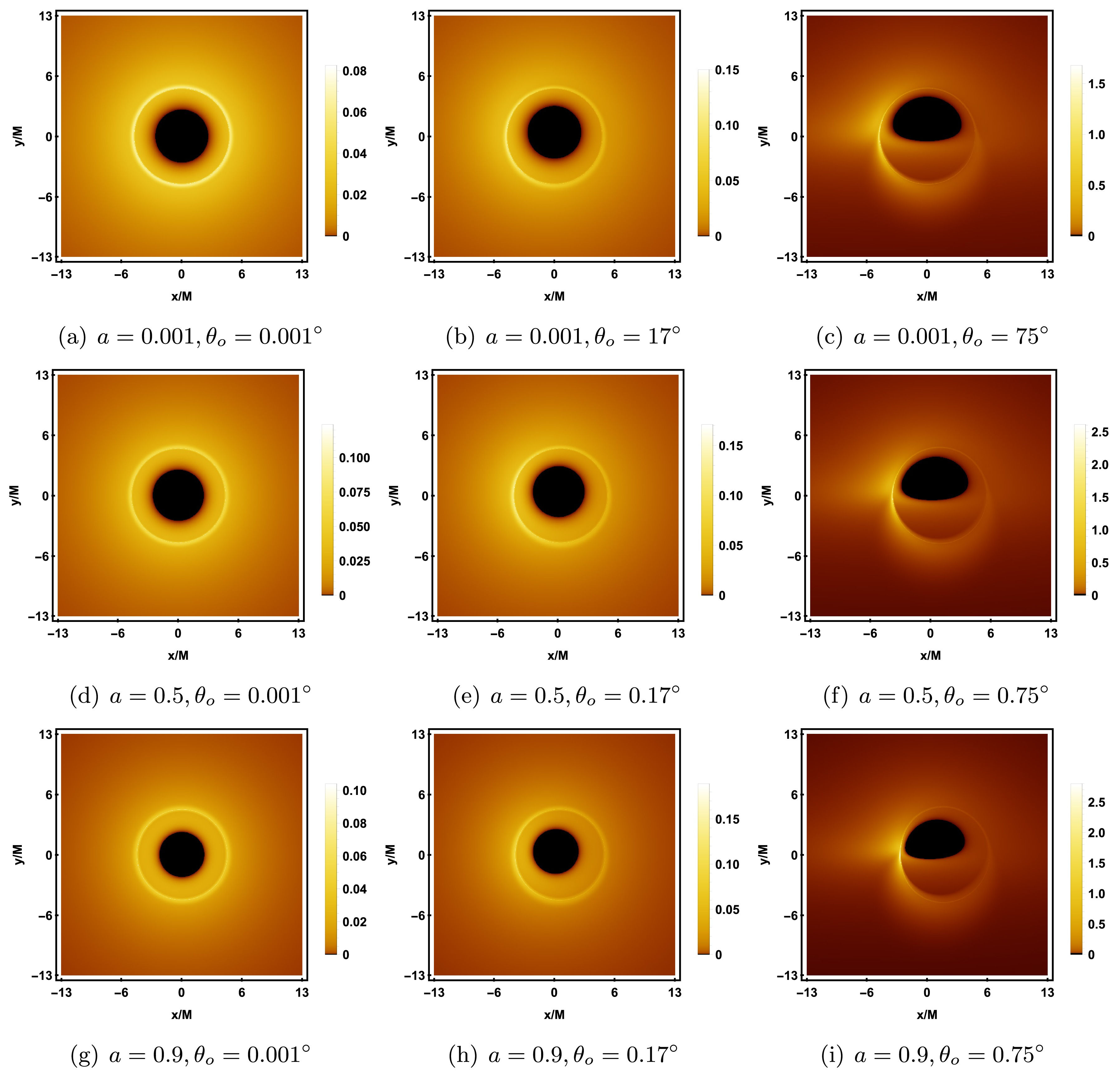
Figure 11. (color online) Rotating black hole shadow with a prograde thin accretion disk in KR gravity. Each row, from top to bottom, corresponds to the rotation parameter
$ a = 0.001, 0.5, 0.9 $ , and each column, from left to right, corresponds to the observer's inclination angle$ \theta_o = 0.001^{\circ}, 17^{\circ}, 75^{\circ} $ . The other parameters are fixed as$ M = 1, \lambda = 0.1, {\cal{G}} = 0.9 $ .It is important to note that in the optical image of a black hole, variations in the number of times light ray traverses the accretion disk result in distinct images due to the cumulative effect of light intensity at each passage. Specifically, the primary image (direct image) corresponds to the case where
$ n = 1 $ , the secondary image (lensed image) corresponds to$ n = 2 $ , and paths involving three or more crossings correspond to higher-order images (photon rings). The definition of photon rings is generally subject to variation. For instance, according to Refs. [84, 85], the photon ring includes all images located outside the direct image. In contrast, Refs. [41, 42] define the term more narrowly, referring specifically to images situated beyond both the primary and secondary images. In this work, we adopt the definition provided in the latter set of references. To better distinguish between direct and lensed images in the shadow image, we plot the observed fluxes in Figure 12. The yellow, blue, and green regions in the image correspond to direct image, lensed image and the photon ring, respectively. For all parameter values, the range of direct image is the widest, while the photon ring always lies within the range of lensed image. When$ \theta_o \to 0^{\circ} $ (the first column), lensed image and the photon ring form concentric circular structures, with the center located at the origin and coinciding with the center of the inner shadow. As a increases, the radius of the rings slightly decreases but remains symmetrical. When$ \theta_o $ increases to$ 17^{\circ} $ (the second column), lensed image and the photon ring shift towards the negative half of the y-axis, and the rings are no longer symmetrical. As$ \theta_o $ further increases to$ 75^{\circ} $ (the third column), both the inner shadow, lensed image, and the photon ring undergo significant deformation. The range of lensed image greatly increases, mainly concentrated in the lower half of the screen, with less distribution in the upper half. Additionally, the photon ring becomes more prominent in the lower half of the screen. These deformations become more pronounced as a increases. The above analysis indicates that the observer's inclination angle$ \theta_o $ has a significant impact on the black hole shadow image, especially the size of the inner shadow and the distribution of the lensed image.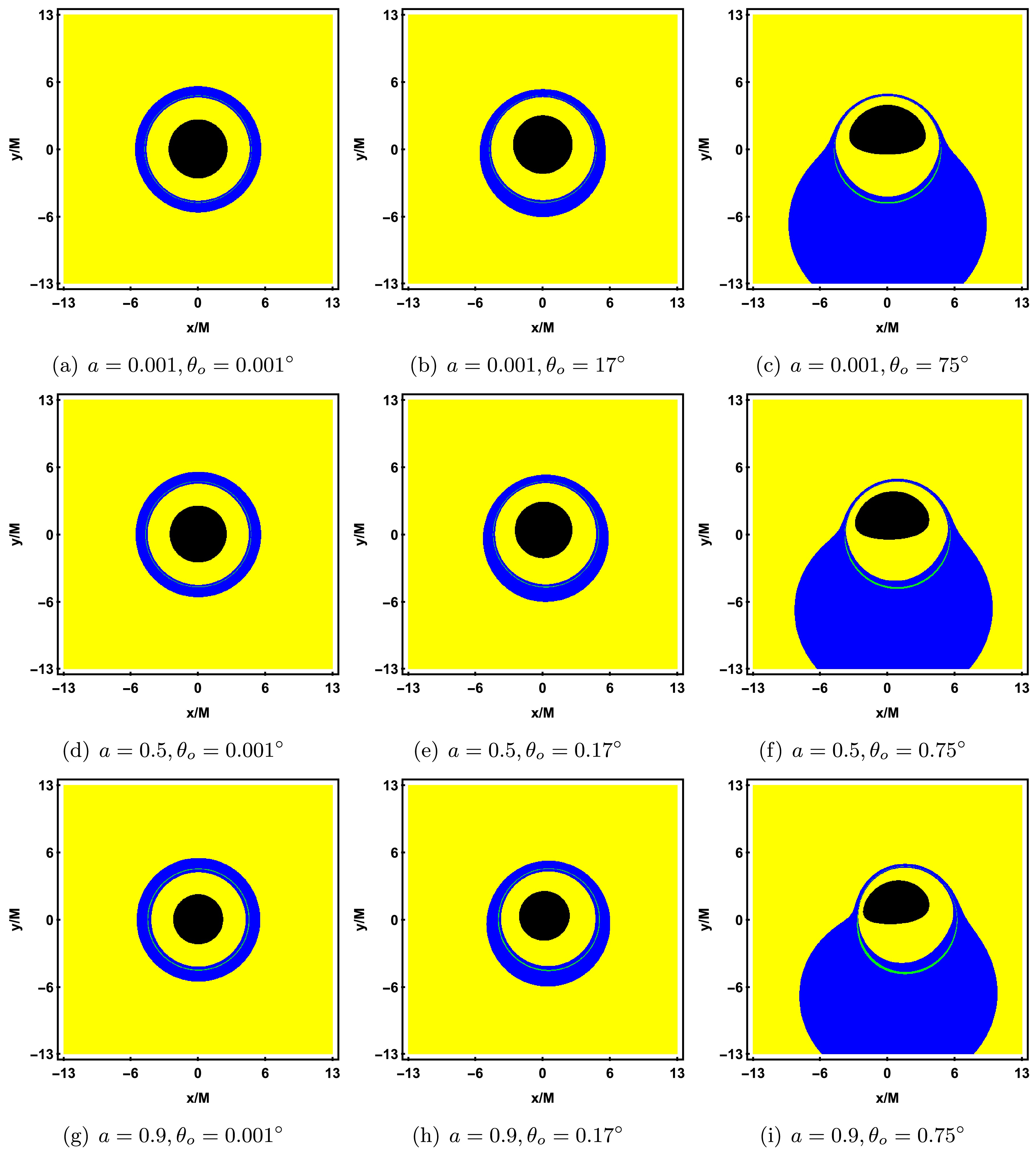
Figure 12. (color online) Observed flux of the direct image, lensed image, and photon ring with a prograde thin accretion disk in KR gravity. The black, yellow, blue, and green regions correspond to the inner shadow, direct image, lensed image, and photon ring, respectively. Each row shows the gradual increase of the rotation parameter a, and each column shows the gradual increase of the observer's inclination angle
$ \theta_o $ . The other parameters are fixed as$ M = 1, \lambda = 0.1, {\cal{G}} = 0.9 $ .The impact of the spontaneous Lorentz symmetry violation parameter λ on the black hole shadow image is shown in Figure 13, with the corresponding observed flux shown in Figure 14. Each row, from top to bottom, corresponds to
$ \lambda = 0.1, 0.5, 0.9 $ , and each column, from left to right, corresponds to the observer inclination angles$ \theta_o = 0.001^{\circ}, 17^{\circ}, 75^{\circ} $ , with other parameters fixed as$ M = 1, a = 0.001, {\cal{G}} = 0.9 $ . From Figure 13, it can be seen that as λ increases, the radii of the inner shadow and the photon ring both decrease, but the brightness of the photon ring gradually increases. As$ \theta_o $ increases, the inner shadow undergoes noticeable deformation, evolving from a symmetric circle into a D-shaped. When$ \theta_o \to 0^{\circ} $ (the first column), the brightness distribution of the photon ring is uniform; when$ \theta_o $ increases to$ 75^{\circ} $ (the third column), a crescent-shaped bright area appears on the left side of the photon ring, with the intensity clearly higher than the right side, making the direct image and lensed image from the accretion disk clearly distinguishable. Furthermore, at$ \theta_o = 75^{\circ} $ , a slight clockwise rotation of the inner shadow around the x-axis can also be observed. From Figure 14, it can be seen that an increase in λ slightly reduces the range of lensed image and the photon ring. As$ \theta_o $ increases, the lensed image gradually shifts towards the lower half of the screen, and when$ \theta_o = 75^{\circ} $ , the range of lensed image even extends beyond the screen. Meanwhile, the photon ring in the upper half of the screen becomes sparse, while the photon ring in the lower half becomes more prominent.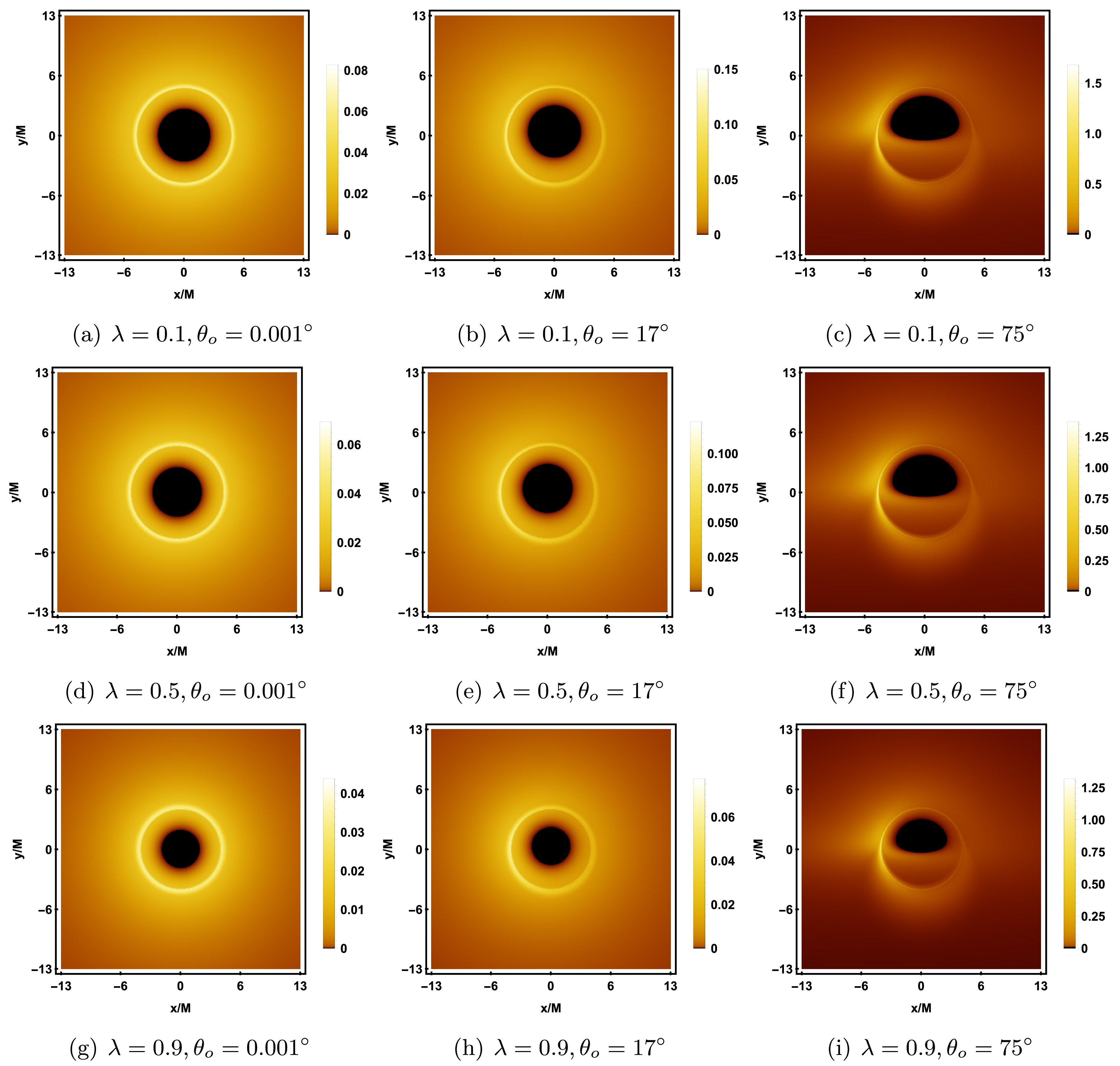
Figure 13. (color online) Rotating black hole shadow with a prograde thin accretion disk in KR gravity. Each row, from top to bottom, corresponds to
$ \lambda = 0.1, 0.5, 0.9 $ , and each column, from left to right, corresponds to the observer's inclination angle$ \theta_o = 0.001^{\circ}, 17^{\circ}, 75^{\circ} $ . The other parameters are fixed as$ M = 1, a = 0.001, {\cal{G}} = 0.9 $ .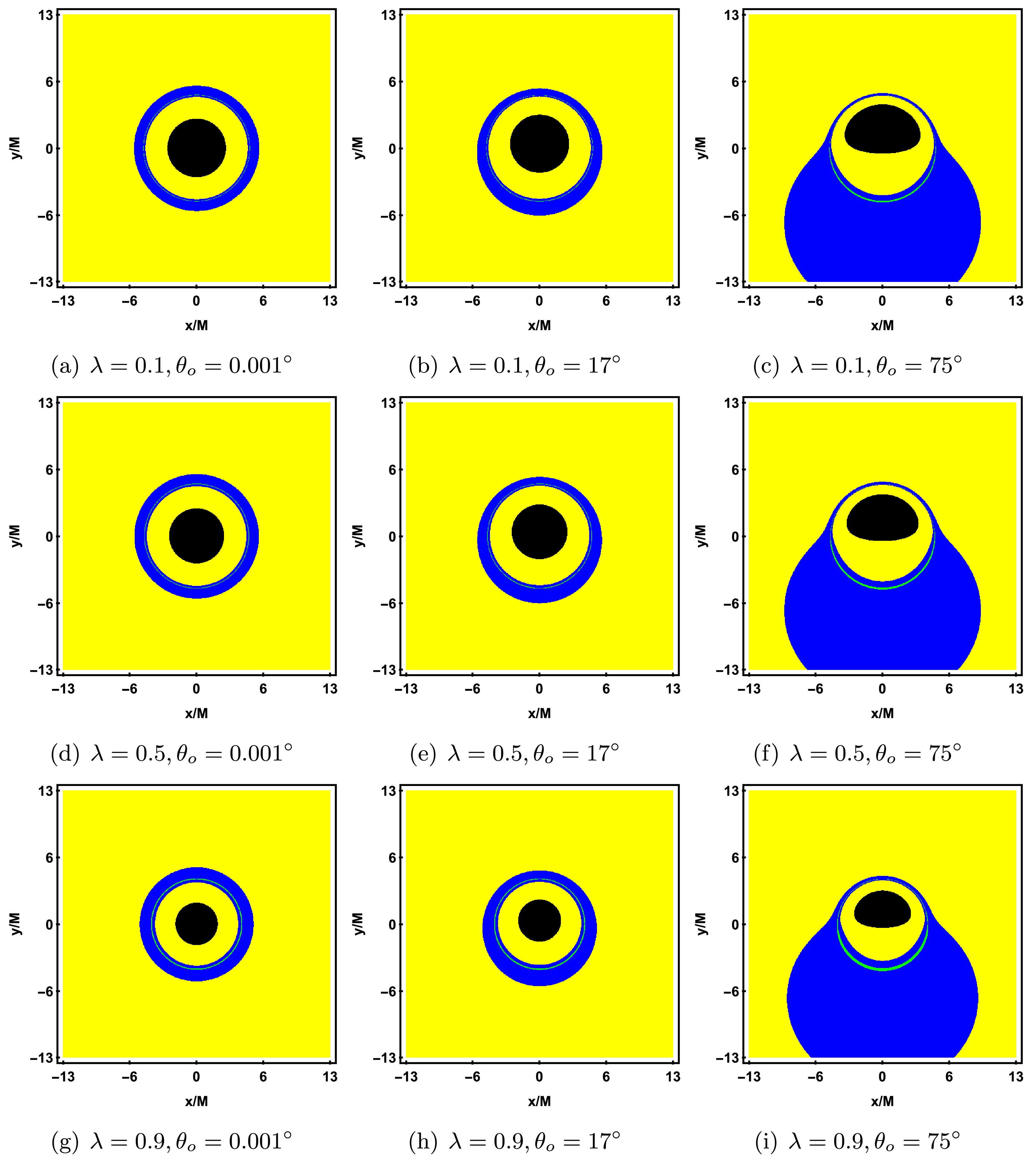
Figure 14. (color online) Observed flux of the direct image, lensed image, and photon ring with a prograde thin accretion disk in KR gravity. The black, yellow, blue, and green regions correspond to the inner shadow, direct image, lensed image, and photon ring, respectively. Each row shows the gradual increase of λ, and each column shows the gradual increase of the observer's inclination angle
$ \theta_o $ . The other parameters are fixed as$ M = 1, a = 0.001, {\cal{G}} = 0.9 $ .Next, we will focus on discussing the impact of the spontaneous Lorentz symmetry violation parameter
$ {\cal{G}} $ on the black hole shadow image. As shown in Figure 15, with the increase in$ {\cal{G}} $ , both the size of the inner shadow and the radius of the photon ring decrease significantly, but their shapes remain nearly unchanged. Additionally, from the colorbar, it can be seen that the image's brightness decreases. As the observer's inclination angle$ \theta_o $ increases, the shape of the inner shadow gradually changes from a circle to an ellipse and eventually evolves into a D-shaped. Similar to the cases of a and λ, when$ \theta_o = 75^{\circ} $ , due to the Doppler effect, the brightness on the left side of the photon ring is significantly higher than that on the right side. The corresponding observed flux of Figure 15 is shown in Figure 16. It can be observed that when$ {\cal{G}} $ and$ \theta_o $ are small, the photon ring in the image is not prominent. As$ {\cal{G}} $ and$ \theta_o $ increase, the lensed image and the photon ring gradually shift towards the lower half of the screen, and the brightness of the photon ring becomes more prominent.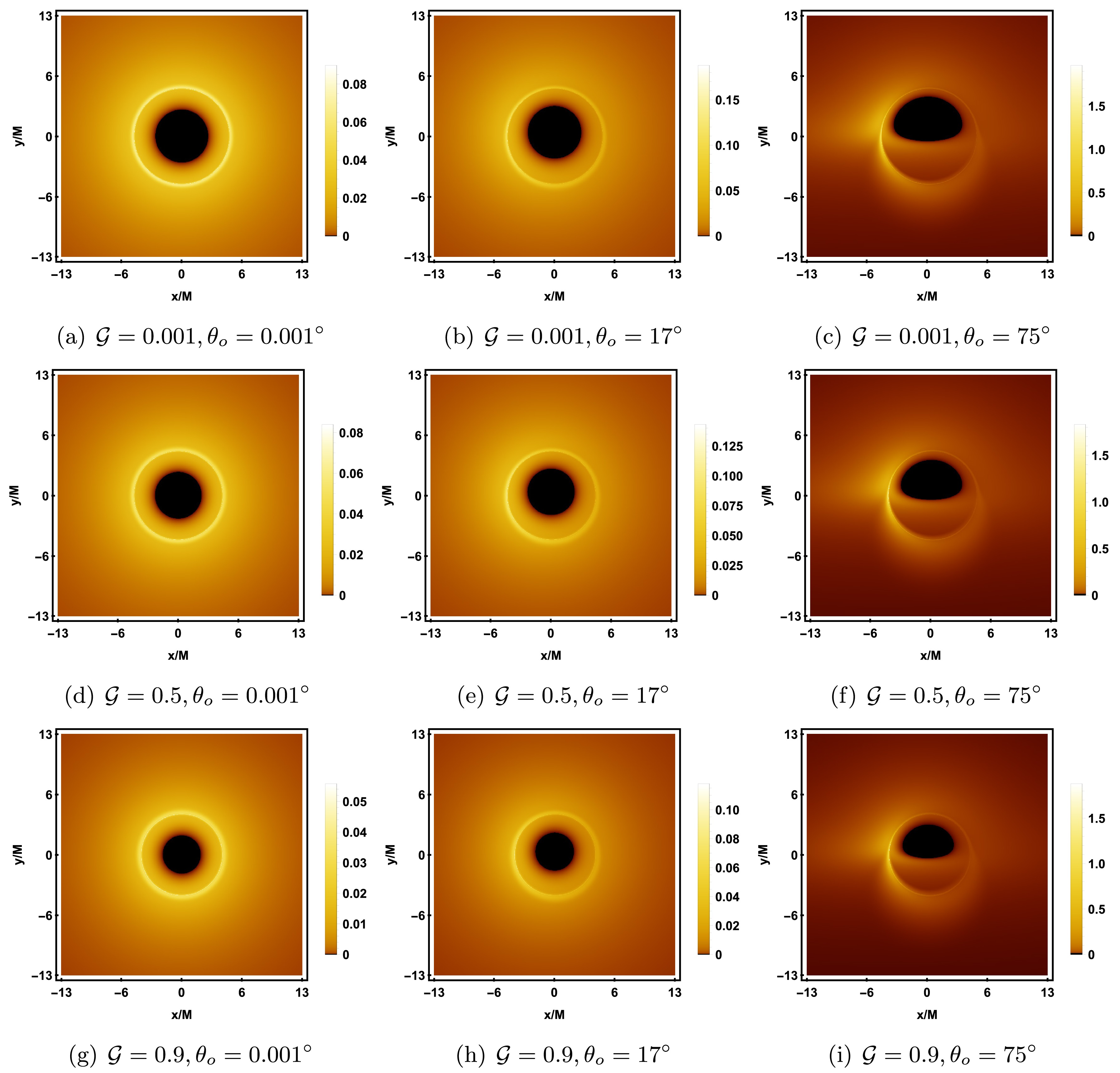
Figure 15. (color online) Rotating black hole shadow with a prograde thin accretion disk in KR gravity. Each row, from top to bottom, corresponds to
$ {\cal{G}} = 0.001, 0.5, 0.9 $ , and each column, from left to right, corresponds to the observer's inclination angle$ \theta_o = 0.001^{\circ}, 17^{\circ}, 75^{\circ} $ . The other parameters are fixed as$ M = 1, a = 0.1, \lambda = 0.9 $ .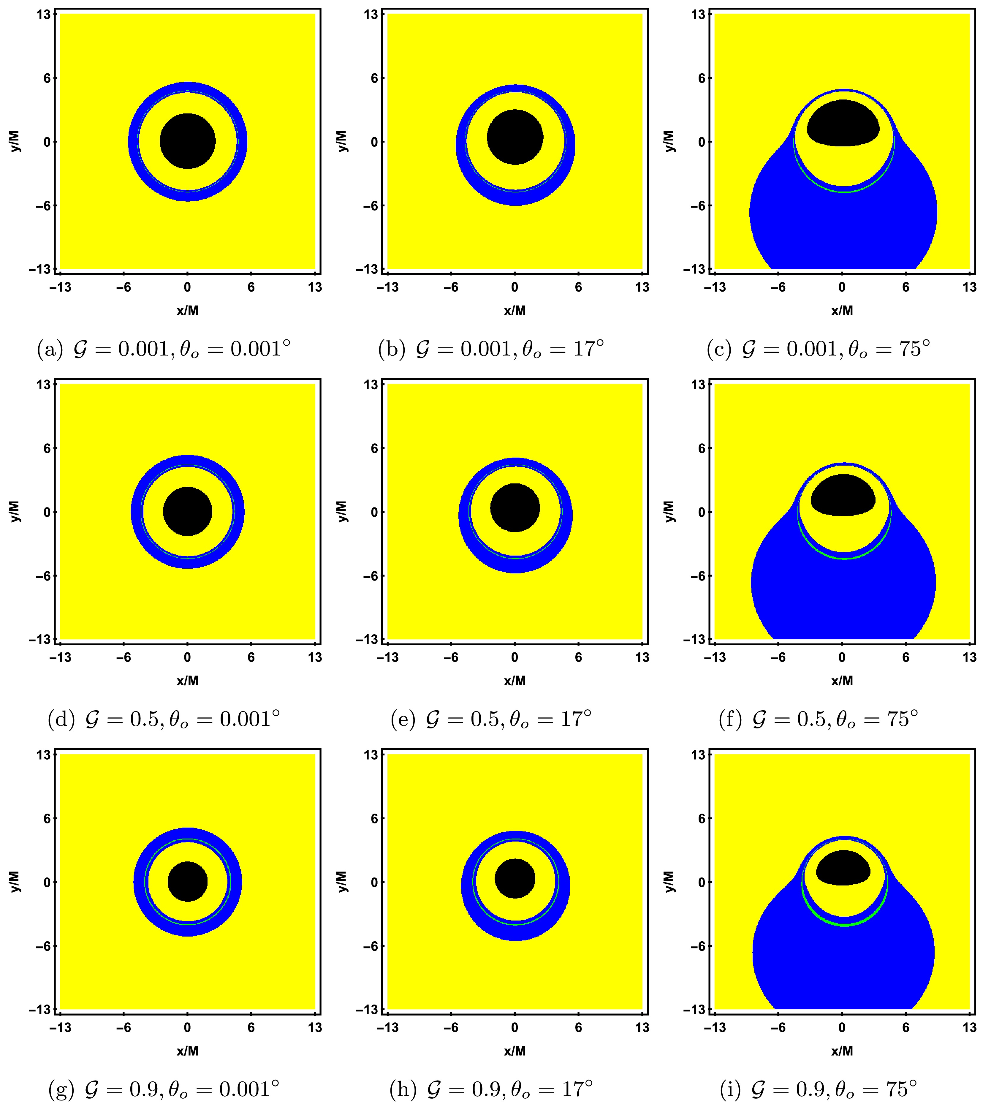
Figure 16. (color online) Observed flux of the direct image, lensed image, and photon ring with a prograde thin accretion disk in KR gravity. The black, yellow, blue, and green regions correspond to the inner shadow, direct image, lensed image, and photon ring, respectively. Each row shows the gradual increase of
$ {\cal{G}} $ , and each column shows the gradual increase of the observer's inclination angle$ \theta_o $ . The other parameters are fixed as$ M = 1, a = 0.1, \lambda = 0.9 $ .At the end of this section, we will discuss the black hole shadow image illuminated by a retrograde accretion disk as the light source, i.e., the motion direction of the accreting material is opposite to the black hole's spin direction. By comparing the shadow images of the retrograde (Figure 17) and prograde (Figure 13, the third column) accretion disks, it can be observed that, under the same parameter settings, the inner shadow of both cases is identical in shape and size. However, for the retrograde accretion disk, the crescent bright region of the photon ring appears on the right side, which is the opposite of the prograde accretion disk. This is due to the different motion directions of the accreting material relative to the observer, leading to a change in the direction of Doppler redshift. Similar to the prograde accretion disk, as λ or
$ {\cal{G}} $ increases, the size of the inner shadow decreases, the distinguishability of the photon ring improves, and the brightness of the crescent bright region increases accordingly.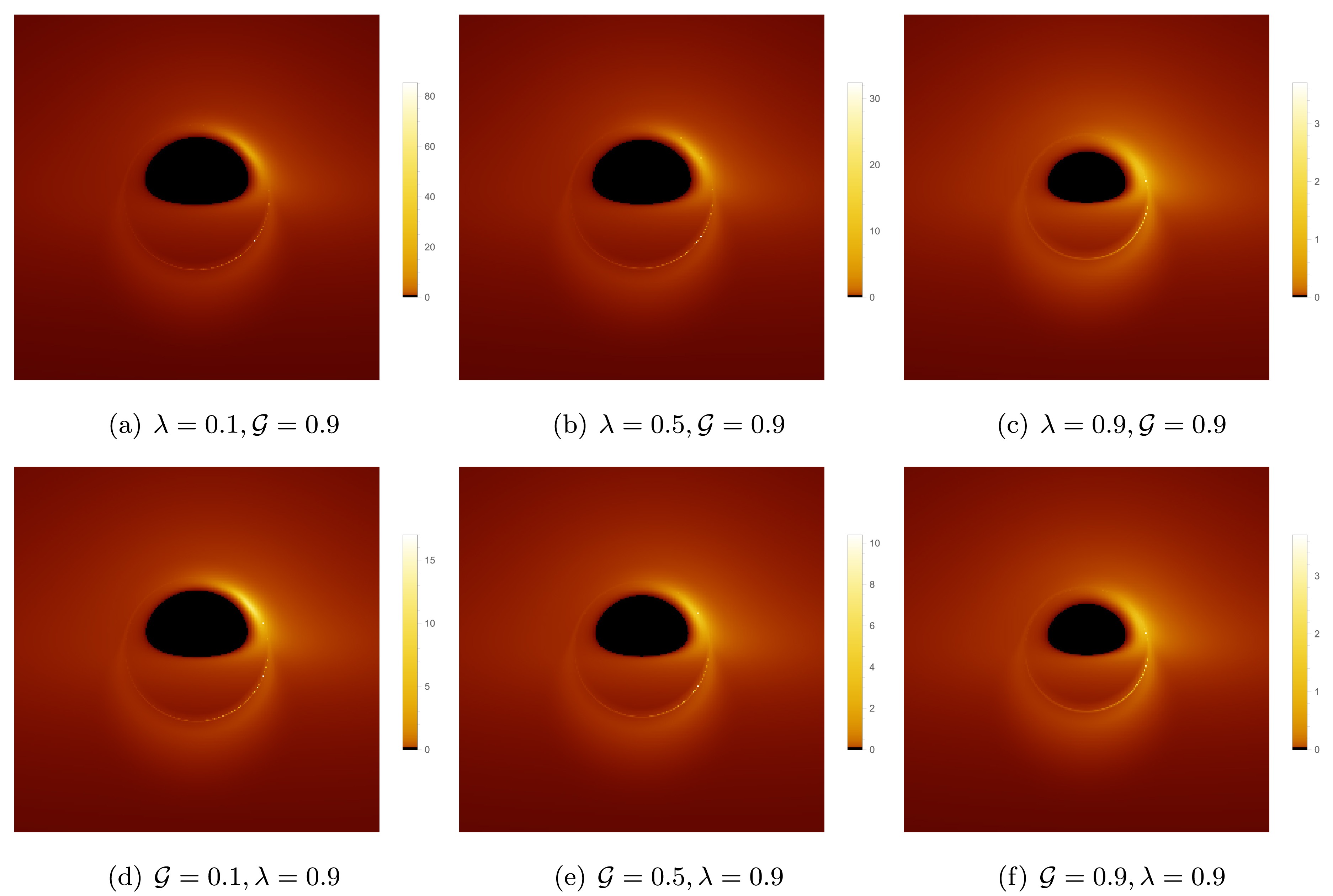
Figure 17. (color online) Rotating black hole shadow with a retrograde thin accretion disk in KR gravity. The first row, from left to right, corresponds to
$ \lambda = 0.1, 0.5, 0.9 $ , and the second row, from left to right, corresponds to$ {\cal{G}} = 0.1, 0.5, 0.9 $ . The other parameters are fixed as$ M = 1 $ ,$ a = 0.001 $ , and$ \theta_o = 75^{\circ} $ . -
In this subsection, we will use numerical methods to plot the shadow image of a rotating black hole with a thin accretion disk in KR gravity. The geometric structure of the spacetime (8) is primarily determined by the rotation parameter a, the spontaneous Lorentz symmetry violation parameters λ, and
$ {\cal{G}} $ . Therefore, we will focus on how these parameters affect the features of the black hole shadow image. In the numerical calculations, the observer's distance is set to$ r_o = 500M $ , with the coordinate axes units taken as$ x/M $ and$ y/M $ , where$ M = 1 $ represents the black hole mass. The observer inclination angles$ \theta_o $ are set to$ 0.001^{\circ} $ ,$ 17^{\circ} $ , and$ 75^{\circ} $ .The black hole shadow images corresponding to different rotation parameters a are shown in Fig. 11. From top to bottom in each row, the values of a are
$ 0.001 $ ,$ 0.5 $ , and$ 0.9 $ , with$ \lambda = 0.1 $ and$ {\cal{G}} = 0.9 $ fixed. In the center of each image, a black region, called the inner shadow, can be observed [45]. When the photon directly falls into the event horizon without passing through the equatorial plane, we have$ {\cal{I}}_{o} = 0 $ according to Eq. (59), and hence, the pixels corresponding to the inner shadow are black, indicating that the black hole's strong gravity prevents the photon from escaping. Outside the inner shadow, there is a luminous ring, called the photon ring. When the observer's inclination angle$ \theta_o = 0.001^{\circ} $ (the first column), the inner shadow appears as a perfect circle, and the photon ring is a symmetric circle with the same center as the coordinate origin. This is because as$ \theta_o \to 0^{\circ} $ , the observer's line of sight becomes perpendicular to the equatorial plane, aligned with the accretion disk and and the black hole's rotation axis. In this case, the radial velocity of each point on the accretion disk relative to the observer is nearly zero, and there is almost no Doppler redshift; the observed redshift is primarily due to gravitational redshift. When$ \theta_o = 17^{\circ} $ (the second column), the inner shadow undergoes slight deformation and is no longer a perfect circle, with the center of the photon ring shifting downward to the right. As$ \theta_o $ increases to$ 75^{\circ} $ (the third column), the deformation of the inner shadow becomes more pronounced, appearing in a D-shaped, and a crescent-shaped bright area appears on the left side of the photon ring, with brightness significantly higher than the surrounding regions. The prograde accretion disk causes the photons from the left side to move toward the observer, producing a blueshift, increasing the photon energy and brightening the shadow image. The photons from the right side move away from the observer, producing a redshift, decreasing the photon energy and dimming the shadow image. Furthermore, by comparing the images in each row, we can see that as a increases, the inner shadow gradually becomes smaller, while the brightness of the photon ring increases. In particular, when$ \theta_o = 75^{\circ} $ , increasing a further enhances the dragging effect of the black hole on the background celestial sphere and the Doppler effect, causing the size and brightness of the crescent bright area on the left to gradually increase.
Figure 11. (color online) Rotating black hole shadow with a prograde thin accretion disk in KR gravity. Each row, from top to bottom, corresponds to the rotation parameter
$ a = 0.001,\, 0.5,\, 0.9 $ , and each column, from left to right, corresponds to the observer's inclination angle$ \theta_o = 0.001^{\circ},\, 17^{\circ},\, 75^{\circ} $ . The other parameters are fixed as$ M = 1,\, \lambda = 0.1,\, {\cal{G}} = 0.9 $ .It is important to note that in the optical image of a black hole, variations in the number of times light ray traverses the accretion disk result in distinct images due to the cumulative effect of light intensity at each passage. Specifically, the primary image (direct image) corresponds to the case where
$ n = 1 $ , the secondary image (lensed image) corresponds to$ n = 2 $ , and paths involving three or more crossings correspond to higher-order images (photon rings). The definition of photon rings is generally subject to variation. For instance, according to Refs. [84, 85], the photon ring includes all images located outside the direct image. In contrast, Refs. [41, 42] define the term more narrowly, referring specifically to images situated beyond both the primary and secondary images. In this work, we adopt the definition provided in the latter set of references. To better distinguish between direct and lensed images in the shadow image, we plot the observed fluxes in Fig. 12. The yellow, blue, and green regions in the image correspond to direct image, lensed image and the photon ring, respectively. For all parameter values, the range of direct image is the widest, while the photon ring always lies within the range of lensed image. When$ \theta_o \to 0^{\circ} $ (the first column), lensed image and the photon ring form concentric circular structures, with the center located at the origin and coinciding with the center of the inner shadow. As a increases, the radius of the rings slightly decreases but remains symmetrical. When$ \theta_o $ increases to$ 17^{\circ} $ (the second column), lensed image and the photon ring shift toward the negative half of the y-axis, and the rings are no longer symmetrical. As$ \theta_o $ further increases to$ 75^{\circ} $ (the third column), both the inner shadow, lensed image, and the photon ring undergo significant deformation. The range of lensed image greatly increases, mainly concentrated in the lower half of the screen, with less distribution in the upper half. Additionally, the photon ring becomes more prominent in the lower half of the screen. These deformations become more pronounced as a increases. The above analysis indicates that the observer's inclination angle$ \theta_o $ has a significant impact on the black hole shadow image, particularly the size of the inner shadow and the distribution of the lensed image.
Figure 12. (color online) Observed flux of the direct image, lensed image, and photon ring with a prograde thin accretion disk in KR gravity. The black, yellow, blue, and green regions correspond to the inner shadow, direct image, lensed image, and photon ring, respectively. Each row shows the gradual increase of the rotation parameter a, and each column shows the gradual increase of the observer's inclination angle
$ \theta_o $ . The other parameters are fixed as$ M = 1,\, \lambda = 0.1,\, {\cal{G}} = 0.9 $ .The impact of the spontaneous Lorentz symmetry violation parameter λ on the black hole shadow image is shown in Fig. 13, with the corresponding observed flux shown in Fig. 14. Each row, from top to bottom, corresponds to
$ \lambda = 0.1,\, 0.5,\, 0.9 $ , and each column, from left to right, corresponds to the observer inclination angles$ \theta_o = 0.001^{\circ},\, 17^{\circ},\, 75^{\circ} $ , with other parameters fixed as$ M = 1,\, a = 0.001,\, {\cal{G}} = 0.9 $ . From Fig. 13, it can be seen that as λ increases, the radii of the inner shadow and the photon ring both decrease, but the brightness of the photon ring gradually increases. As$ \theta_o $ increases, the inner shadow undergoes noticeable deformation, evolving from a symmetric circle into a D-shaped. When$ \theta_o \to 0^{\circ} $ (the first column), the brightness distribution of the photon ring is uniform; when$ \theta_o $ increases to$ 75^{\circ} $ (the third column), a crescent-shaped bright area appears on the left side of the photon ring, with the intensity clearly higher than the right side, making the direct image and lensed image from the accretion disk clearly distinguishable. Furthermore, at$ \theta_o = 75^{\circ} $ , a slight clockwise rotation of the inner shadow around the x-axis can be observed. From Fig. 14, it can be seen that an increase in λ slightly reduces the range of the lensed image and the photon ring. As$ \theta_o $ increases, the lensed image gradually shifts toward the lower half of the screen, and when$ \theta_o = 75^{\circ} $ , the range of lensed image even extends beyond the screen. Meanwhile, the photon ring in the upper half of the screen becomes sparse, while the photon ring in the lower half becomes more prominent.
Figure 13. (color online) Rotating black hole shadow with a prograde thin accretion disk in KR gravity. Each row, from top to bottom, corresponds to
$ \lambda = 0.1,\, 0.5,\, 0.9 $ , and each column, from left to right, corresponds to the observer's inclination angle$ \theta_o = 0.001^{\circ},\, 17^{\circ},\, 75^{\circ} $ . The other parameters are fixed as$ M = 1,\, a = 0.001,\, {\cal{G}} = 0.9 $ .
Figure 14. (color online) Observed flux of the direct image, lensed image, and photon ring with a prograde thin accretion disk in KR gravity. The black, yellow, blue, and green regions correspond to the inner shadow, direct image, lensed image, and photon ring, respectively. Each row shows the gradual increase of λ, and each column shows the gradual increase of the observer's inclination angle
$ \theta_o $ . The other parameters are fixed as$ M = 1,\, a = 0.001,\, {\cal{G}} = 0.9 $ .Next, we will focus on discussing the impact of the spontaneous Lorentz symmetry violation parameter
$ {\cal{G}} $ on the black hole shadow image. As shown in Fig. 15, with the increase in$ {\cal{G}} $ , both the size of the inner shadow and the radius of the photon ring decrease significantly, but their shapes remain nearly unchanged. Additionally, from the colorbar, it can be seen that the image's brightness decreases. As the observer's inclination angle$ \theta_o $ increases, the shape of the inner shadow gradually changes from a circle to an ellipse and eventually evolves into a D-shaped. Similar to the cases of a and λ, when$ \theta_o = 75^{\circ} $ , due to the Doppler effect, the brightness on the left side of the photon ring is significantly higher than that on the right side. The corresponding observed flux of Fig. 15 is shown in Fig. 16. It can be observed that when$ {\cal{G}} $ and$ \theta_o $ are small, the photon ring in the image is not prominent. As$ {\cal{G}} $ and$ \theta_o $ increase, the lensed image and the photon ring gradually shift toward the lower half of the screen, and the brightness of the photon ring becomes more prominent.
Figure 15. (color online) Rotating black hole shadow with a prograde thin accretion disk in KR gravity. Each row, from top to bottom, corresponds to
$ {\cal{G}} = 0.001,\; 0.5,\; 0.9 $ , and each column, from left to right, corresponds to the observer's inclination angle$ \theta_o = 0.001^{\circ}, $ $ 17^{\circ},\, 75^{\circ} $ . The other parameters are fixed as$ M = 1,\, a = 0.1,\, \lambda = 0.9 $ .
Figure 16. (color online) Observed flux of the direct image, lensed image, and photon ring with a prograde thin accretion disk in KR gravity. The black, yellow, blue, and green regions correspond to the inner shadow, direct image, lensed image, and photon ring, respectively. Each row shows the gradual increase of
$ {\cal{G}} $ , and each column shows the gradual increase of the observer's inclination angle$ \theta_o $ . The other parameters are fixed as$ M = 1,\, a = 0.1,\, \lambda = 0.9 $ .At the end of this section, we will discuss the black hole shadow image illuminated by a retrograde accretion disk as the light source, i.e., the motion direction of the accreting material is opposite to the black hole's spin direction. By comparing the shadow images of the retrograde (Fig. 17) and prograde (Fig. 13, the third column) accretion disks, it can be observed that, under the same parameter settings, the inner shadow of both cases is identical in shape and size. However, for the retrograde accretion disk, the crescent bright region of the photon ring appears on the right side, which is the opposite of the prograde accretion disk. This is due to the different motion directions of the accreting material relative to the observer, leading to a change in the direction of Doppler redshift. Similar to the prograde accretion disk, as λ or
$ {\cal{G}} $ increases, the size of the inner shadow decreases, the distinguishability of the photon ring improves, and the brightness of the crescent bright region increases accordingly.
Figure 17. (color online) Rotating black hole shadow with a retrograde thin accretion disk in KR gravity. The first row, from left to right, corresponds to
$ \lambda = 0.1,\, 0.5,\, 0.9 $ , and the second row, from left to right, corresponds to$ {\cal{G}} = 0.1,\, 0.5,\, 0.9 $ . The other parameters are fixed as$ M = 1 $ ,$ a = 0.001 $ , and$ \theta_o = 75^{\circ} $ . -
The relative motion between the accreting material and the observer generates a Doppler effect, which may significantly affect the features of the black hole shadow image. Therefore, it is crucial to study the distribution of the redshift factor
$ \chi_n $ on the imaging plane. Figures 18 and 19 show the distribution of the redshift factor for direct and lensed images under the prograde accretion disk model. Each row corresponds to observer inclination angles$ \theta_o = 0.001^{\circ},\, 17^{\circ},\, 75^{\circ} $ from top to bottom. In the figures, red and blue represent redshift and blueshift, respectively, with the intensity of the color reflecting the strength of the redshift, which is linearly related to the intensity. For direct images, the black region at the center of the figure represents the inner shadow; for lensed images, the black region at the center represents both the inner shadow and part of the direct image. It can be observed that the size of the inner shadow depends on the parameters a,$ {\cal{G}} $ , and λ, which determine the spacetime geometry, while the shape of the inner shadow depends on the observer's inclination angle$ \theta_o $ .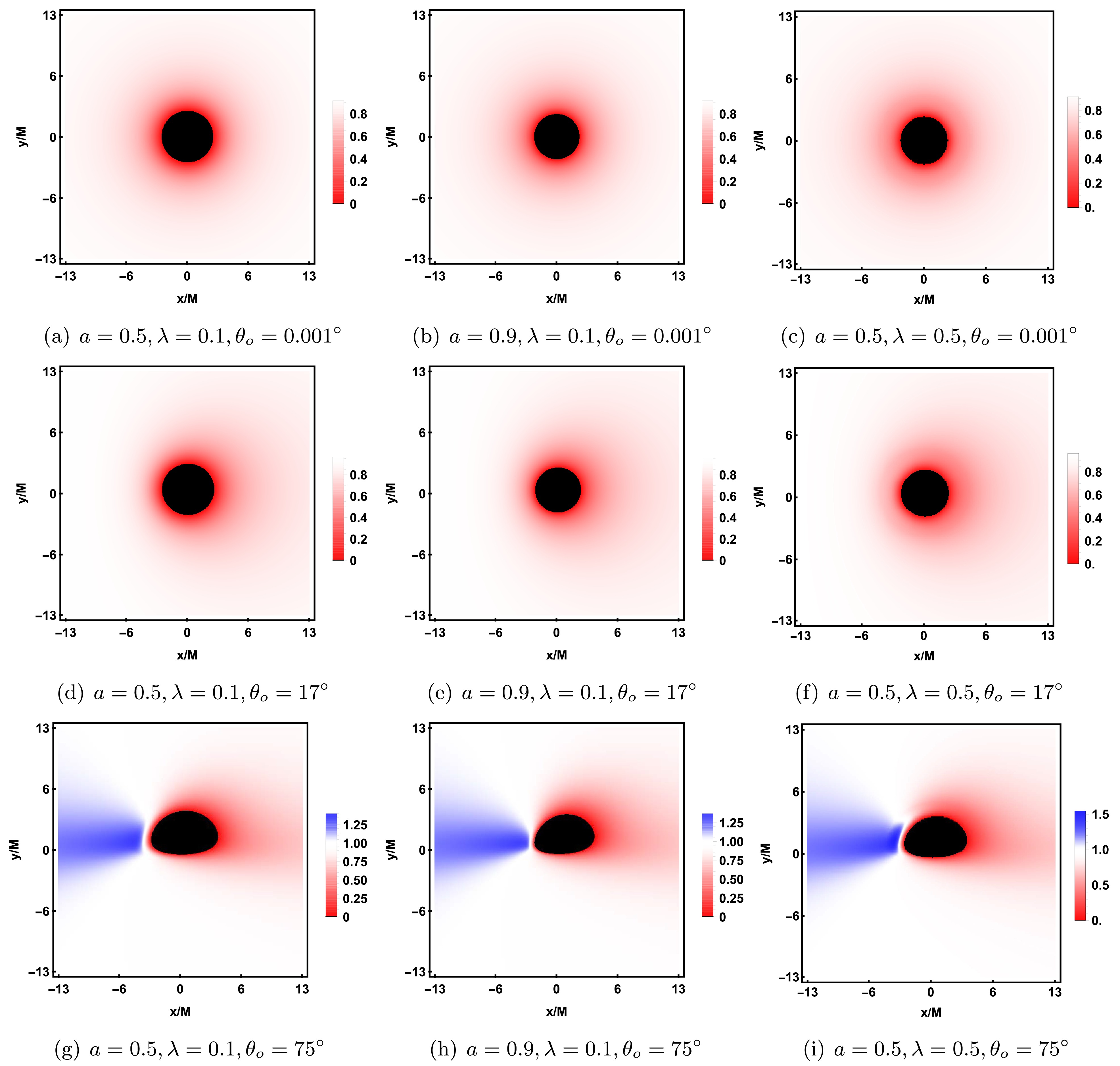
Figure 18. Redshift factor distribution of direct image with a prograde thin accretion disk. The black region represents the inner shadow, while red and blue indicate redshift and blueshift, respectively. The intensity of the color reflects the strength of the redshift, which is linearly related to the intensity. From the first row to the third row, the observer's inclination angle is
$ \theta_o = 0.001^{\circ},\, 17^{\circ},\, 75^{\circ} $ , with the other parameters fixed as$ M = 1 $ and$ {\cal{G}} = 0.9 $ .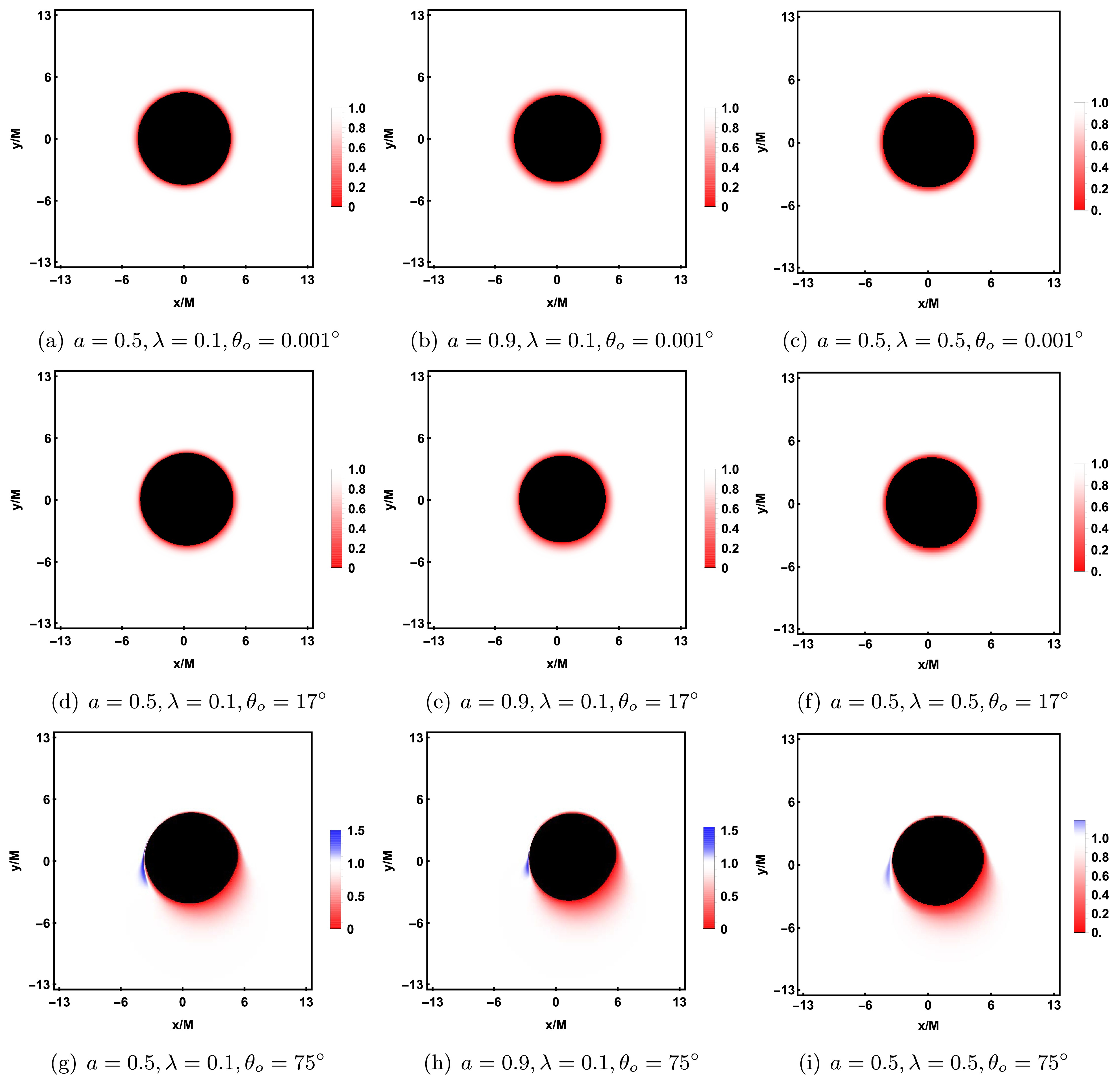
Figure 19. Redshift factor distribution of lensed images with a prograde thin accretion disk. From the first row to the third row, the observer's inclination angle is
$ \theta_o = 0.001^{\circ},\, 17^{\circ},\, 75^{\circ} $ , with the other parameters fixed as$ M = 1 $ and$ {\cal{G}} = 0.9 $ .Whether they are direct or lensed images, when
$ \theta_o = 0.001^{\circ} $ or$ 17^{\circ} $ , only redshift appears without any blueshift. The redshift range for direct images is wider, while for lensed images, only a thin "red ring" appears. This is because when$ \theta_o $ is small, the radial velocity component of the accreting material relative to the observer is small, and gravitational redshift dominates. When$ \theta_o $ increases to$ 75^{\circ} $ , the Doppler effect significantly intensifies, causing a blueshift region to appear in the image. Among these, the blueshift in the direct images is particularly prominent, while the lensed images only forms a crescent-shaped slight blueshift, corresponding to the crescent bright area in the photon ring of the black hole shadow. The blueshift is concentrated on the left side of the inner shadow, while the redshift is primarily concentrated on the right side. This phenomenon is determined by the prograde motion of the accretion disk. It is worth noting that for direct images, when$ \theta_o = 75^{\circ} $ (the third row of Fig. 18), by keeping other parameters unchanged, increasing a or λ causes the blueshift region to move to the left side of the screen, further separating from the redshift region.The redshift factor distribution of direct and lensed images under the retrograde accretion disk is shown in Fig. 20. Compared to the prograde accretion disk, the redshift and blueshift regions are reversed. This phenomenon arises from the change in the direction of motion of the accreting material relative to the observer in the retrograde accretion disk, which causes the redshift and blueshift regions to be reversed due to the Doppler effect. In the retrograde accretion disk, the blueshift region appears on the right side of the image, corresponding to the crescent bright area of the photon ring in the black hole shadow image, which is also on the right. Similar to the prograde case, as λ or
$ {\cal{G}} $ increases, the size of the inner shadow gradually decreases, but its shape remains almost unchanged. Simultaneously, the blueshift region of direct image shifts to the right, further separating from the redshift region.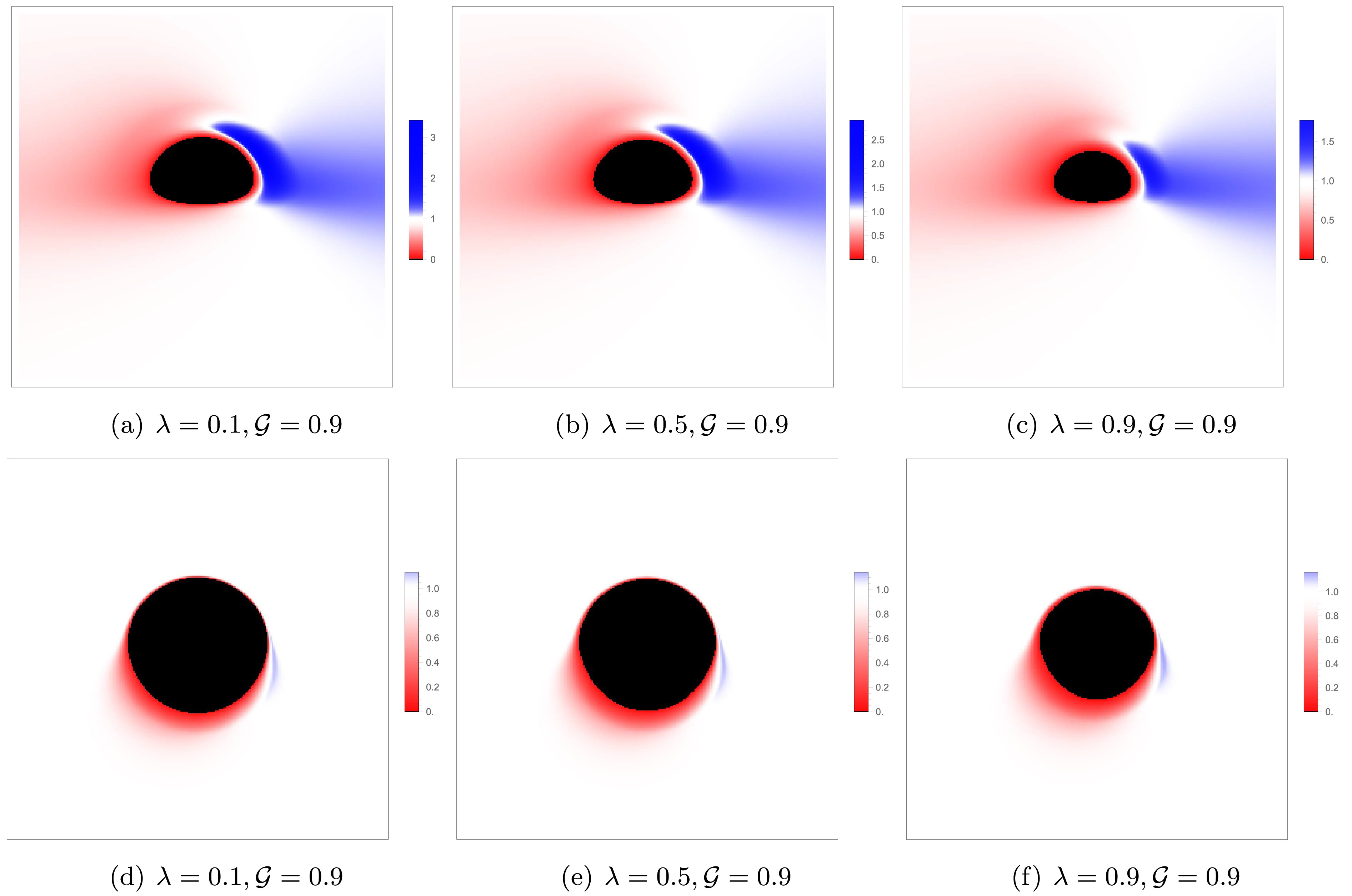
Figure 20. Redshift factor distribution of direct and lensed images with a retrograde thin accretion disk. The other parameters are fixed as
$ M = 1 $ ,$ a = 0.001 $ and$ \theta_o = 75^{\circ} $ . -
The relative motion between the accreting material and the observer generates a Doppler effect, which may significantly affect the features of the black hole shadow image. Therefore, it is crucial to study the distribution of the redshift factor
$ \chi_n $ on the imaging plane. Figures 18 and 19 show the distribution of the redshift factor for direct and lensed images under the prograde accretion disk model. Each row corresponds to observer inclination angles$ \theta_o = 0.001^{\circ}, 17^{\circ}, 75^{\circ} $ from top to bottom. In the figures, red and blue represent redshift and blueshift, respectively, with the intensity of the color reflecting the strength of the redshift, which is linearly related to the intensity. For direct images, the black region at the center of the figure represents the inner shadow; for lensed images, the black region at the center represents both the inner shadow and part of the direct image. It can be observed that the size of the inner shadow depends on the parameters a,$ {\cal{G}} $ , and λ, which determine the spacetime geometry, while the shape of the inner shadow depends on the observer's inclination angle$ \theta_o $ .
Figure 18. Redshift factor distribution of direct image with a prograde thin accretion disk. The black region represents the inner shadow, while red and blue indicate redshift and blueshift, respectively. The intensity of the color reflects the strength of the redshift, which is linearly related to the intensity. From the first row to the third row, the observer's inclination angle is
$ \theta_o = 0.001^{\circ}, 17^{\circ}, 75^{\circ} $ , with the other parameters fixed as$ M = 1 $ and$ {\cal{G}} = 0.9 $ .
Figure 19. Redshift factor distribution of lensed images with a prograde thin accretion disk. From the first row to the third row, the observer's inclination angle is
$ \theta_o = 0.001^{\circ}, 17^{\circ}, 75^{\circ} $ , with the other parameters fixed as$ M = 1 $ and$ {\cal{G}} = 0.9 $ .Whether they are direct or lensed images, when
$ \theta_o = 0.001^{\circ} $ or$ 17^{\circ} $ , only redshift appears without any blueshift. The redshift range for direct images is wider, while for lensed images, only a thin "red ring" appears. This is because when$ \theta_o $ is small, the radial velocity component of the accreting material relative to the observer is small, and gravitational redshift dominates. When$ \theta_o $ increases to$ 75^{\circ} $ , the Doppler effect significantly intensifies, causing a blueshift region to appear in the image. Among these, the blueshift in the direct images is particularly prominent, while the lensed images only forms a crescent-shaped slight blueshift, corresponding to the crescent bright area in the photon ring of the black hole shadow. The blueshift is concentrated on the left side of the inner shadow, while the redshift is primarily concentrated on the right side. This phenomenon is determined by the prograde motion of the accretion disk. It is worth noting that for direct images, when$ \theta_o = 75^{\circ} $ (the third row of Figure 18), by keeping other parameters unchanged, increasing a or λ causes the blueshift region to move to the left side of the screen, further separating from the redshift region.The redshift factor distribution of direct and lensed images under the retrograde accretion disk is shown in Figure 20. Compared to the prograde accretion disk, the redshift and blueshift regions are reversed. This phenomenon arises from the change in the direction of motion of the accreting material relative to the observer in the retrograde accretion disk, which causes the redshift and blueshift regions to be reversed due to the Doppler effect. In the retrograde accretion disk, the blueshift region appears on the right side of the image, corresponding to the crescent bright area of the photon ring in the black hole shadow image, which is also on the right. Similar to the prograde case, as λ or
$ {\cal{G}} $ increases, the size of the inner shadow gradually decreases, but its shape remains almost unchanged. At the same time, the blueshift region of direct image shifts to the right, further separating from the redshift region.
Figure 20. Redshift factor distribution of direct and lensed images with a retrograde thin accretion disk. The other parameters are fixed as
$ M = 1 $ ,$ a = 0.001 $ and$ \theta_o = 75^{\circ} $ . -
The groundbreaking achievements of the EHT have driven numerical simulations of black hole shadows. In this paper, we study the shadow images of rotating black holes in KR gravity based on backward ray-tracing, with a focus on the effects of the observer's inclination angle
$ \theta_o $ , the rotation parameter a, and the spontaneous Lorentz symmetry violation parameters λ and$ {\cal{G}} $ on the shadow image. Firstly, in the ZAMO frame, we use stereographic projection to explore the shadow characteristics of the KR rotating black hole and attempt to constrain black hole parameters by comparing with observational data from M87 and Sgr A*. Next, considering the case of a spherical light source, we plot the black hole shadow images for different values of$ {\cal{G}} $ and λ. Finally, under the assumption that there is an optically and geometrically thin accretion disk in the black hole's equatorial plane, we study the shadow images and redshift factor distributions for prograde and retrograde accretion disks.The results show that the size and shape of the black hole shadow are closely related to the parameters
$ (a, \lambda, {\cal{G}}) $ . With other parameters fixed, as the rotation parameter a increases, the shadow gradually transforms from a perfect circle to a D-shaped one. The increase in the spontaneous Lorentz symmetry violation parameters λ and$ {\cal{G}} $ causes the shadow to shrink, i.e., the size of the shadow decreases, but the overall shape remains mostly unchanged. By comparing with the observational data of M87 and Sgr A*, it is found that changes in λ and$ {\cal{G}} $ significantly affect the estimated range of the shadow's angular diameter$ {\cal{D}} $ , but the values always remain within the$ 1\sigma $ confidence interval of the M87 and Sgr A* observations. To further narrow the parameter range, future studies still need to incorporate additional conditions for analysis. In the case of a spherical light source, the backward ray tracing technique can precisely determine the shadow shape on the observer's screen. The study shows that the image always consists of a black, nearly circular region and a white circular ring, corresponding to the black hole's inner shadow and the Einstein ring. As$ {\cal{G}} $ increases, the shape of the inner shadow remains nearly circular, but its radius gradually decreases. As λ increases, the inner shadow gradually shrinks, its deformation becomes more significant, and the surrounding celestial sphere exhibits slight distortions due to the dragging effect. Meanwhile, the Einstein ring breaks at the top and bottom, separating into multiple arc segments.On the other hand, we studied the black hole shadow image illuminated by the accretion disk as the light source, assuming the accretion disk lies on the equatorial plane and is both optically and geometrically thin. For rotating black holes in KR gravity, we focused on analyzing the effects of the parameters
$ (\theta_o, a, \lambda, {\cal{G}}) $ on the inner shadow, photon ring, and redshift factor distribution. The study found that$ \theta_o $ has a significant impact on the shape of the inner shadow, while$ (a, \lambda, {\cal{G}}) $ primarily affect the size of the inner shadow. When$ \theta_o \to 0^{\circ} $ , the inner shadow is a perfect circle, and the photon ring forms a symmetric ring with their centers coinciding. As$ \theta_o $ increases, the inner shadow gradually deforms, and when$ \theta_o = 75^{\circ} $ , the inner shadow takes on a D-shape. It is noteworthy that at this point, a crescent-shaped bright region appears on the left side of the photon ring, attributed to the more pronounced Doppler effect due to a larger observer inclination angle. As a increases, the size of the inner shadow gradually decreases, but the brightness of the photon ring significantly increases, making it more distinguishable. Interestingly, a larger a causes a slight counterclockwise rotation of the inner shadow around the x-axis. The effects of λ and$ {\cal{G}} $ on the size of the inner shadow are similar, and whether the accretion disk is prograde or retrograde, the increase of both parameters reduces the size of the inner shadow and photon ring.In addition, we studied the redshift of direct and lensed images produced by the accretion disk. The results show that as
$ \theta_o $ increases, both redshift and blueshift are amplified. When$ \theta_o $ is small (such as$ 0.001^{\circ} $ and$ 17^{\circ} $ ), there is only redshift and no blueshift for both direct and lensed images. At this point, a significant "red ring" appears at the edge of the inner shadow, caused by the light emitted by particles in the critical plunging orbit, and the small$ \theta_o $ leads to gravitational redshift dominating, thus no blueshift is observed. In this case, due to the lack of sharpness in the light intensity distribution, direct and lensed images are difficult to distinguish. As$ \theta_o $ increases to$ 75^{\circ} $ , the enhancement of Doppler redshift causes a noticeable blueshift in the image, making direct and lensed images distinguishable. The prograde accreting material causes the blueshifte on the left and the redshifte on the right. Meanwhile, increasing a or λ further separates the redshift and blueshift regions in direct images, but the effect on lensed images is not significant. A similar phenomenon also occurs in the retrograde accretion disk, but in the retrograde case, the positions of the redshift and blueshift regions are reversed. -
The groundbreaking achievements of the EHT have driven numerical simulations of black hole shadows. In this paper, we study the shadow images of rotating black holes in KR gravity based on backward ray-tracing, with a focus on the effects of the observer's inclination angle
$ \theta_o $ , the rotation parameter a, and the spontaneous Lorentz symmetry violation parameters λ and$ {\cal{G}} $ on the shadow image. Firstly, in the ZAMO frame, we use stereographic projection to explore the shadow characteristics of the KR rotating black hole and attempt to constrain black hole parameters by comparing with observational data from M87 and Sgr A*. Next, considering the case of a spherical light source, we plot the black hole shadow images for different values of$ {\cal{G}} $ and λ. Finally, under the assumption that there is an optically and geometrically thin accretion disk in the black hole's equatorial plane, we study the shadow images and redshift factor distributions for prograde and retrograde accretion disks.The results show that the size and shape of the black hole shadow are closely related to the parameters
$ (a, \lambda, {\cal{G}}) $ . With other parameters fixed, as the rotation parameter a increases, the shadow gradually transforms from a perfect circle to a D-shaped one. The increase in the spontaneous Lorentz symmetry violation parameters λ and$ {\cal{G}} $ causes the shadow to shrink, i.e., the size of the shadow decreases, but the overall shape remains mostly unchanged. By comparing with the observational data of M87 and Sgr A*, it is found that changes in λ and$ {\cal{G}} $ significantly affect the estimated range of the shadow's angular diameter$ {\cal{D}} $ , but the values always remain within the$ 1\sigma $ confidence interval of the M87 and Sgr A* observations. To further narrow the parameter range, future studies still need to incorporate additional conditions for analysis. In the case of a spherical light source, the backward ray tracing technique can precisely determine the shadow shape on the observer's screen. The study shows that the image always consists of a black, nearly circular region and a white circular ring, corresponding to the black hole's inner shadow and the Einstein ring. As$ {\cal{G}} $ increases, the shape of the inner shadow remains nearly circular, but its radius gradually decreases. As λ increases, the inner shadow gradually shrinks, its deformation becomes more significant, and the surrounding celestial sphere exhibits slight distortions due to the dragging effect. Meanwhile, the Einstein ring breaks at the top and bottom, separating into multiple arc segments.On the other hand, we studied the black hole shadow image illuminated by the accretion disk as the light source, assuming the accretion disk lies on the equatorial plane and is both optically and geometrically thin. For rotating black holes in KR gravity, we focused on analyzing the effects of the parameters
$ (\theta_o, a, \lambda, {\cal{G}}) $ on the inner shadow, photon ring, and redshift factor distribution. The study found that$ \theta_o $ has a significant impact on the shape of the inner shadow, while$ (a, \lambda, {\cal{G}}) $ primarily affect the size of the inner shadow. When$ \theta_o \to 0^{\circ} $ , the inner shadow is a perfect circle, and the photon ring forms a symmetric ring with their centers coinciding. As$ \theta_o $ increases, the inner shadow gradually deforms, and when$ \theta_o = 75^{\circ} $ , the inner shadow takes on a D-shaped. It is noteworthy that at this point, a crescent-shaped bright region appears on the left side of the photon ring, attributed to the more pronounced Doppler effect due to a larger observer inclination angle. As a increases, the size of the inner shadow gradually decreases, but the brightness of the photon ring significantly increases, making it more distinguishable. Interestingly, a larger a causes a slight counterclockwise rotation of the inner shadow around the x-axis. The effects of λ and$ {\cal{G}} $ on the size of the inner shadow are similar, and whether the accretion disk is prograde or retrograde, the increase of both parameters reduces the size of the inner shadow and photon ring.In addition, we also studied the redshift of direct and lensed images produced by the accretion disk. The results show that as
$ \theta_o $ increases, both redshift and blueshift are amplified. When$ \theta_o $ is small (such as$ 0.001^{\circ} $ and$ 17^{\circ} $ ), there is only redshift and no blueshift for both direct and lensed images. At this point, a significant "red ring" appears at the edge of the inner shadow, caused by the light emitted by particles in the critical plunging orbit, and the small$ \theta_o $ leads to gravitational redshift dominating, thus no blueshift is observed. In this case, due to the lack of sharpness in the light intensity distribution, direct and lensed images are difficult to distinguish. As$ \theta_o $ increases to$ 75^{\circ} $ , the enhancement of Doppler redshift causes a noticeable blueshift in the image, making direct and lensed images distinguishable. The prograde accreting material causes the blueshifte on the left and the redshifte on the right. Meanwhile, increasing a or λ further separates the redshift and blueshift regions in direct images, but the effect on lensed images is not significant. A similar phenomenon also occurs in the retrograde accretion disk, but in the retrograde case, the positions of the redshift and blueshift regions are reversed.
Shadow images of a rotating black hole in Kalb-Ramond gravity surrounded by the thin accretion disk
- Received Date: 2025-08-01
- Available Online: 2026-03-15
Abstract: We investigate the shadow image of rotating black holes in Kalb-Ramond gravity using backward ray-tracing techniques. We consider two primary emission models: a spherical source and a optically and geometrically thin accretion disk. The results show that enhanced black hole rotation parameter a amplifies the shadow's departure from circular symmetry, whereas spontaneous Lorentz symmetry-breaking parameters ${\cal{G}}$ and λ suppress the shadow radius. For accretion disk models, observer inclination angle $\theta_o$ predominantly governs the inner shadow morphology and photon ring brightness asymmetry, while a, ${\cal{G}}$, and λ primarily modulate the inner shadow scale. An increase in $\theta_o$ induces a morphological transition of the inner shadow from a circular to a D-shaped geometry, accompanied by enhanced brightness in a crescent-shaped region on the left side. Meanwhile, increasing the values of a, ${\cal{G}}$, or λ decrease the dimensions of the shadow. Furthermore, higher inclination angles $\theta_o$ further enhance spectral differentiation, that is, low inclination angles exhibit exclusively redshifted emission. Additionally, those at high inclination angles produce blueshifted components in both direct and lensed images. These characteristic signatures provide observational discriminators between rotating Kalb-Ramond black holes and alternative spacetime.


 DownLoad: