


 Abstract
 HTML
HTML Reference
 Related
 PDF
PDF


-
Numerous astronomical observations indicate that supermassive black holes typically exist at the centers of large galaxies. Gravitational-wave observatories have detected mergers of stellar-mass black holes, confirming the existence of these celestial objects [1]. The Event Horizon Telescope (EHT) images of the supermassive black holes M87* [2] and Sgr A* [3] provide direct visual evidence for the existence of black holes. Recently, polarization measurements by the EHT have further revealed the detailed structure and radiation processes of magnetized plasma near the event horizon [3, 4], offering a new means of studying accretion physics and spacetime geometry in strong gravitational fields. In fact, the shadow observed by the EHT is not a direct image of the event horizon but a projection of the strong gravitational lensing effect of a black hole [5]. This phenomenon originates from unstable circular photon orbits, for which the boundary between photon capture and escape appears visually as a central dark region surrounded by a bright photon ring [6]. Because the size and shape of shadows depend sensitively on the geometric structure of the background spacetime [7], high-resolution observations of these shadows provide a unique opportunity to test gravitational theories.
In General Relativity (GR), solutions of Einstein's field equations inevitably encounter the singularity problem, which refers to a point at which the curvature scalar approaches infinity within the event horizon of a black hole. Spacetime singularities are widely regarded as manifestations of the incompleteness of GR, which may be resolved by a quantum theory of gravity or by modifications to gravitational theory [8, 9]. Remarkably, Bardeen obtained a black hole solution without a singularity [10], which can be interpreted as a gravitationally collapsed magnetic monopole arising from a specific form of nonlinear electrodynamics [11]. Subsequently, Hayward proposed a static, spherically symmetric black hole solution that accounts for the boundedness and regularity of curvature invariants in regular spacetime [12]. Thereafter, additional regular black holes were proposed, including the Ayón-Beato–García black hole [13], the Berej–Matyjasek–Tryniecki–Woronowicz black hole [14], and the rotating Bardeen black hole [15]. Naturally, the physical properties of such regular black holes have attracted considerable attention. Research has addressed diverse aspects, including dynamical stability, quasinormal modes of scalar-field perturbations, weak gravitational lensing effects, and the geodesic motion of test particles [16−20].
On the other hand, non-commutative spacetime has emerged as a significant topic in gravitational theory, serving as a potential approach to quantizing gravity [21]. In particular, it has been demonstrated that non-commutativity can provide a solution to the central singularities affecting the Schwarzschild and Reissner–Nordström metrics [22−24]. The corresponding non-commutative counterparts of these metrics are derived by incorporating non-commutativity solely into the matter source, while leaving the Einstein action unchanged [25]. Consequently, the central singularity is replaced by a regular region represented by a self-gravitating droplet of anisotropic fluid. Several methods have been developed to realize non-commutative spacetime in gravitational theories [26−31]. Studies have demonstrated that regularity within the framework of GR can be attained by modifying the matter source, specifically by replacing the Dirac delta function with either a Gaussian distribution [22] or a Lorentzian distribution [32]. Relevant studies have examined the properties of objects in non-commutative spacetime, including thermodynamic properties, quasinormal modes, and the geometric structure of spacetime [25, 33−39]. When this metric is applied to astrophysical black holes within classical General Relativity, the parameter λ effectively acts as a macroscopic deformation scale characterizing the regularized fluid core, rather than as a direct measure of the Planckian quantum gravity scale. Because the black hole shadow is an intrinsic observational signature strictly governed by this background geometry, employing shadows as anchors to extract the imprint of λ provides a direct pathway for understanding the macroscopic physical characteristics of such regularized spacetimes in strong gravitational fields.
In our universe, a black hole is generally surrounded by a luminous accretion flow, which is crucial for imaging black holes. Because most of the light received from a black hole originates from the accretion flow, the observational characteristics of its shadow and photon ring depend on the position and morphology of the accretion flow [40]. Simplified accretion models, such as spherically symmetric and thin-disk accretion models [41−45], can capture the basic features of black hole images. However, compared with realistic astrophysical environments, these models still have limitations. In particular, astronomical observations suggest that Sgr A* and M87 are low-luminosity active galactic nuclei (AGN), which are typically associated with radiatively inefficient accretion flows (RIAFs) [2]. These flows are expected to be geometrically thick and optically thin because of their low accretion rates and advection-dominated dynamics. In the RIAF model, the vertically averaged electron number density and temperature exhibit approximate power-law distributions with radius [46]. Simultaneously, the RIAF model simplifies the treatment of processes including outflows, non-thermal particles, and full general relativistic magnetohydrodynamics (GRMHD). Owing to its distinct physical basis and high compatibility with the results of GRMHD simulations, this phenomenological framework has successfully reproduced the submillimeter spectrum and the main imaging characteristics of objects such as M87* [4]. Therefore, based on the RIAF model, several notable findings have already been obtained in studies of black hole images [47, 48].
Based on non-commutative Schwarzschild spacetime, several results have been obtained regarding black hole shadows and their optical observational images. However, the relevant studies have been conducted within the frameworks of simplified spherical accretion and geometrically thin-disk models [49]. In realistic astrophysical environments such as low-luminosity active galactic nuclei, black holes are typically surrounded by geometrically thick, advection-dominated accretion flows. Therefore, treating the non-commutative Schwarzschild metric as an analytically tractable model for a regular black hole with an effective macroscopic deformation, we investigate its imaging characteristics within the framework of the radiatively inefficient accretion flow (RIAF) model. Through numerical solutions of the GRRT equations, we analyze the intensity distributions and morphological features of black hole shadows and photon rings across different values of the deformation parameter λ, inclination angles, and observation frequencies. We aim to investigate how macroscopic spacetime regularizations interact with realistic, geometrically thick plasma backgrounds and whether the effects of metric modifications remain consistent across different accretion models. In addition, we examine differences in image features under the assumptions of isotropic and anisotropic synchrotron emission. The relevant results provide a comprehensive reference framework and an analytical benchmark for diagnosing effective spacetime deformations in strong gravitational fields.
The remainder of this paper is organized as follows. In Sec. II, we briefly introduce the geometric properties of static black holes based on spacetime non-commutativity. In Sec. III, we establish the theoretical framework for the radiation mechanisms and GRRT. In Sec. IV, we present the phenomenological model of a geometrically thick RIAF and the projection technique for mapping the celestial sphere onto the observation plane. In Sec. V, we present the numerical results. Finally, in Sec. VI, we summarize the main results of this study.
-
Numerous astronomical observations indicate that supermassive black holes typically exist at the centers of large galaxies. Gravitational-wave observatories have detected mergers of stellar-mass black holes, confirming the existence of these celestial objects [1]. The Event Horizon Telescope (EHT) images of the supermassive black holes M87* [2] and Sgr A* [3] provide direct visual evidence for the existence of black holes. Recently, polarization measurements by the EHT have further revealed the detailed structure and radiation processes of magnetized plasma near the event horizon [3, 4], offering a new means of studying accretion physics and spacetime geometry in strong gravitational fields. In fact, the shadow observed by the EHT is not a direct image of the event horizon but a projection of the strong gravitational lensing effect of a black hole [5]. This phenomenon originates from unstable circular photon orbits, for which the boundary between photon capture and escape appears visually as a central dark region surrounded by a bright photon ring [6]. Because the size and shape of shadows depend sensitively on the geometric structure of the background spacetime [7], high-resolution observations of these shadows provide a unique opportunity to test gravitational theories.
In General Relativity (GR), solutions of Einstein's field equations inevitably encounter the singularity problem, which refers to a point at which the curvature scalar approaches infinity within the event horizon of a black hole. Spacetime singularities are widely regarded as manifestations of the incompleteness of GR, which may be resolved by a quantum theory of gravity or by modifications to gravitational theory [8, 9]. Remarkably, Bardeen obtained a black hole solution without a singularity [10], which can be interpreted as a gravitationally collapsed magnetic monopole arising from a specific form of nonlinear electrodynamics [11]. Subsequently, Hayward proposed a static, spherically symmetric black hole solution that accounts for the boundedness and regularity of curvature invariants in regular spacetime [12]. Thereafter, additional regular black holes were proposed, including the Ayón-Beato–García black hole [13], the Berej–Matyjasek–Tryniecki–Woronowicz black hole [14], and the rotating Bardeen black hole [15]. Naturally, the physical properties of such regular black holes have attracted considerable attention. Research has addressed diverse aspects, including dynamical stability, quasinormal modes of scalar-field perturbations, weak gravitational lensing effects, and the geodesic motion of test particles [16−20].
On the other hand, non-commutative spacetime has emerged as a significant topic in gravitational theory, serving as a potential approach to quantizing gravity [21]. In particular, it has been demonstrated that non-commutativity can provide a solution to the central singularities affecting the Schwarzschild and Reissner–Nordström metrics [22−24]. The corresponding non-commutative counterparts of these metrics are derived by incorporating non-commutativity solely into the matter source, while leaving the Einstein action unchanged [25]. Consequently, the central singularity is replaced by a regular region represented by a self-gravitating droplet of anisotropic fluid. Several methods have been developed to realize non-commutative spacetime in gravitational theories [26−31]. Studies have demonstrated that regularity within the framework of GR can be attained by modifying the matter source, specifically by replacing the Dirac delta function with either a Gaussian distribution [22] or a Lorentzian distribution [32]. Relevant studies have examined the properties of objects in non-commutative spacetime, including thermodynamic properties, quasinormal modes, and the geometric structure of spacetime [25, 33−39]. When this metric is applied to astrophysical black holes within classical General Relativity, the parameter λ effectively acts as a macroscopic deformation scale characterizing the regularized fluid core, rather than as a direct measure of the Planckian quantum gravity scale. Because the black hole shadow is an intrinsic observational signature strictly governed by this background geometry, employing shadows as anchors to extract the imprint of λ provides a direct pathway for understanding the macroscopic physical characteristics of such regularized spacetimes in strong gravitational fields.
In our universe, a black hole is generally surrounded by a luminous accretion flow, which is crucial for imaging black holes. Because most of the light received from a black hole originates from the accretion flow, the observational characteristics of its shadow and photon ring depend on the position and morphology of the accretion flow [40]. Simplified accretion models, such as spherically symmetric and thin-disk accretion models [41−45], can capture the basic features of black hole images. However, compared with realistic astrophysical environments, these models still have limitations. In particular, astronomical observations suggest that Sgr A* and M87 are low-luminosity active galactic nuclei (AGN), which are typically associated with radiatively inefficient accretion flows (RIAFs) [2]. These flows are expected to be geometrically thick and optically thin because of their low accretion rates and advection-dominated dynamics. In the RIAF model, the vertically averaged electron number density and temperature exhibit approximate power-law distributions with radius [46]. Simultaneously, the RIAF model simplifies the treatment of processes including outflows, non-thermal particles, and full general relativistic magnetohydrodynamics (GRMHD). Owing to its distinct physical basis and high compatibility with the results of GRMHD simulations, this phenomenological framework has successfully reproduced the submillimeter spectrum and the main imaging characteristics of objects such as M87* [4]. Therefore, based on the RIAF model, several notable findings have already been obtained in studies of black hole images [47, 48].
Based on non-commutative Schwarzschild spacetime, several results have been obtained regarding black hole shadows and their optical observational images. However, the relevant studies have been conducted within the frameworks of simplified spherical accretion and geometrically thin-disk models [49]. In realistic astrophysical environments such as low-luminosity active galactic nuclei, black holes are typically surrounded by geometrically thick, advection-dominated accretion flows. Therefore, treating the non-commutative Schwarzschild metric as an analytically tractable model for a regular black hole with an effective macroscopic deformation, we investigate its imaging characteristics within the framework of the radiatively inefficient accretion flow (RIAF) model. Through numerical solutions of the GRRT equations, we analyze the intensity distributions and morphological features of black hole shadows and photon rings across different values of the deformation parameter λ, inclination angles, and observation frequencies. We aim to investigate how macroscopic spacetime regularizations interact with realistic, geometrically thick plasma backgrounds and whether the effects of metric modifications remain consistent across different accretion models. In addition, we examine differences in image features under the assumptions of isotropic and anisotropic synchrotron emission. The relevant results provide a comprehensive reference framework and an analytical benchmark for diagnosing effective spacetime deformations in strong gravitational fields.
The remainder of this paper is organized as follows. In Sec. II, we briefly introduce the geometric properties of static black holes based on spacetime non-commutativity. In Sec. III, we establish the theoretical framework for the radiation mechanisms and GRRT. In Sec. IV, we present the phenomenological model of a geometrically thick RIAF and the projection technique for mapping the celestial sphere onto the observation plane. In Sec. V, we present the numerical results. Finally, in Sec. VI, we summarize the main results of this study.
-
Numerous astronomical observations indicate that supermassive black holes typically exist at the centers of large galaxies. Gravitational-wave observatories have detected mergers of stellar-mass black holes, confirming the existence of these celestial objects [1]. The Event Horizon Telescope (EHT) images of the supermassive black holes M87* [2] and Sgr A* [3] provide direct visual evidence for the existence of black holes. Recently, polarization measurements by the EHT have further revealed the detailed structure and radiation processes of magnetized plasma near the event horizon [3, 4], offering a new means of studying accretion physics and spacetime geometry in strong gravitational fields. In fact, the shadow observed by the EHT is not a direct image of the event horizon but a projection of the strong gravitational lensing effect of a black hole [5]. This phenomenon originates from unstable circular photon orbits, for which the boundary between photon capture and escape appears visually as a central dark region surrounded by a bright photon ring [6]. Because the size and shape of shadows depend sensitively on the geometric structure of the background spacetime [7], high-resolution observations of these shadows provide a unique opportunity to test gravitational theories.
In General Relativity (GR), solutions of Einstein's field equations inevitably encounter the singularity problem, which refers to a point at which the curvature scalar approaches infinity within the event horizon of a black hole. Spacetime singularities are widely regarded as manifestations of the incompleteness of GR, which may be resolved by a quantum theory of gravity or by modifications to gravitational theory [8, 9]. Remarkably, Bardeen obtained a black hole solution without a singularity [10], which can be interpreted as a gravitationally collapsed magnetic monopole arising from a specific form of nonlinear electrodynamics [11]. Subsequently, Hayward proposed a static, spherically symmetric black hole solution that accounts for the boundedness and regularity of curvature invariants in regular spacetime [12]. Thereafter, additional regular black holes were proposed, including the Ayón-Beato–García black hole [13], the Berej–Matyjasek–Tryniecki–Woronowicz black hole [14], and the rotating Bardeen black hole [15]. Naturally, the physical properties of such regular black holes have attracted considerable attention. Research has addressed diverse aspects, including dynamical stability, quasinormal modes of scalar-field perturbations, weak gravitational lensing effects, and the geodesic motion of test particles [16−20].
On the other hand, non-commutative spacetime has emerged as a significant topic in gravitational theory, serving as a potential approach to quantizing gravity [21]. In particular, it has been demonstrated that non-commutativity can provide a solution to the central singularities affecting the Schwarzschild and Reissner–Nordström metrics [22−24]. The corresponding non-commutative counterparts of these metrics are derived by incorporating non-commutativity solely into the matter source, while leaving the Einstein action unchanged [25]. Consequently, the central singularity is replaced by a regular region represented by a self-gravitating droplet of anisotropic fluid. Several methods have been developed to realize non-commutative spacetime in gravitational theories [26−31]. Studies have demonstrated that regularity within the framework of GR can be attained by modifying the matter source, specifically by replacing the Dirac delta function with either a Gaussian distribution [22] or a Lorentzian distribution [32]. Relevant studies have examined the properties of objects in non-commutative spacetime, including thermodynamic properties, quasinormal modes, and the geometric structure of spacetime [25, 33−39]. When this metric is applied to astrophysical black holes within classical General Relativity, the parameter λ effectively acts as a macroscopic deformation scale characterizing the regularized fluid core, rather than as a direct measure of the Planckian quantum gravity scale. Because the black hole shadow is an intrinsic observational signature strictly governed by this background geometry, employing shadows as anchors to extract the imprint of λ provides a direct pathway for understanding the macroscopic physical characteristics of such regularized spacetimes in strong gravitational fields.
In our universe, a black hole is generally surrounded by a luminous accretion flow, which is crucial for imaging black holes. Because most of the light received from a black hole originates from the accretion flow, the observational characteristics of its shadow and photon ring depend on the position and morphology of the accretion flow [40]. Simplified accretion models, such as spherically symmetric and thin-disk accretion models [41−45], can capture the basic features of black hole images. However, compared with realistic astrophysical environments, these models still have limitations. In particular, astronomical observations suggest that Sgr A* and M87 are low-luminosity active galactic nuclei (AGN), which are typically associated with radiatively inefficient accretion flows (RIAFs) [2]. These flows are expected to be geometrically thick and optically thin because of their low accretion rates and advection-dominated dynamics. In the RIAF model, the vertically averaged electron number density and temperature exhibit approximate power-law distributions with radius [46]. Simultaneously, the RIAF model simplifies the treatment of processes including outflows, non-thermal particles, and full general relativistic magnetohydrodynamics (GRMHD). Owing to its distinct physical basis and high compatibility with the results of GRMHD simulations, this phenomenological framework has successfully reproduced the submillimeter spectrum and the main imaging characteristics of objects such as M87* [4]. Therefore, based on the RIAF model, several notable findings have already been obtained in studies of black hole images [47, 48].
Based on non-commutative Schwarzschild spacetime, several results have been obtained regarding black hole shadows and their optical observational images. However, the relevant studies have been conducted within the frameworks of simplified spherical accretion and geometrically thin-disk models [49]. In realistic astrophysical environments such as low-luminosity active galactic nuclei, black holes are typically surrounded by geometrically thick, advection-dominated accretion flows. Therefore, treating the non-commutative Schwarzschild metric as an analytically tractable model for a regular black hole with an effective macroscopic deformation, we investigate its imaging characteristics within the framework of the radiatively inefficient accretion flow (RIAF) model. Through numerical solutions of the GRRT equations, we analyze the intensity distributions and morphological features of black hole shadows and photon rings across different values of the deformation parameter λ, inclination angles, and observation frequencies. We aim to investigate how macroscopic spacetime regularizations interact with realistic, geometrically thick plasma backgrounds and whether the effects of metric modifications remain consistent across different accretion models. In addition, we examine differences in image features under the assumptions of isotropic and anisotropic synchrotron emission. The relevant results provide a comprehensive reference framework and an analytical benchmark for diagnosing effective spacetime deformations in strong gravitational fields.
The remainder of this paper is organized as follows. In Sec. II, we briefly introduce the geometric properties of static black holes based on spacetime non-commutativity. In Sec. III, we establish the theoretical framework for the radiation mechanisms and GRRT. In Sec. IV, we present the phenomenological model of a geometrically thick RIAF and the projection technique for mapping the celestial sphere onto the observation plane. In Sec. V, we present the numerical results. Finally, in Sec. VI, we summarize the main results of this study.
-
The Schwarzschild metric describes the geometry of a static, spherically symmetric vacuum spacetime. Its line element is given by
$ {\rm d}s^2 = -A(r){\rm d}t^2 + \frac{1}{A(r)}{\rm d}r^2 + r^2\left({\rm d}\theta^2 + \sin^2\theta {\rm d}\varphi^2\right). $
(1) The classical Schwarzschild metric inevitably contains an intrinsic curvature singularity at
$ r=0 $ . To resolve this central singularity, we adopt the framework of spacetime non-commutativity [21, 22], in which the coordinates satisfy the non-commutative algebra$ [x^\mu, x^\nu] = {\rm i}\lambda^{\mu\nu}, $
(2) $ [x^\mu, x^\nu] = {\rm i}\lambda^{\mu\nu}, $
(3) where
$ \lambda^{\mu\nu} $ is an antisymmetric tensor that introduces a microscopic length scale to mitigate the singularity problem. We employ a Lorentzian-smeared energy density [32]$ \rho_{\lambda}(r) = \dfrac{\sqrt{\lambda} M}{\pi^{3 / 2}\left(r^{2} + \pi \lambda\right)^{2}}. $
(4) This distribution has a finite value at
$ r=0 $ , given by$ \rho_{\lambda}(0)= \dfrac{M}{\pi^{7/2}\lambda^{3/2}} $ . Consequently, the energy density remains finite, thereby eliminating the central spacetime singularity within the effective theoretical framework.Solving the Einstein field equations yields the metric function in the form
$ A(r) = 1 - \frac{2\mathcal{M}_{\lambda}(r)}{r}, $
(5) where the mass accumulation function is
$\begin{aligned}[b] \mathcal{M}_{\lambda}(r)=\;&\int_{0}^{r} \rho_{\lambda}\left(r^{\prime}\right) 4 \pi r^{\prime 2} {\rm d} r^{\prime}\\=\;&\frac{2 M}{\pi}\left(\tan ^{-1}\left(\frac{r}{\sqrt{\pi \lambda}}\right)-\frac{r \sqrt{\pi \lambda}}{r^{2}+\pi \lambda}\right)\\=\;& M - \frac{4\sqrt{\lambda} M}{\sqrt{\pi} r} + \mathcal{O}\left(\lambda^{3/2}\right).\end{aligned} $
(6) In the limit
$ \lambda \to 0 $ , the metric reduces to the classical Schwarzschild solution. Expanding this exact solution in the small-λ approximation (i.e.,$ \sqrt{\lambda} \ll M $ ), we obtain the leading-order correction to the metric function$ A(r) = 1 - \frac{2M}{r} + \frac{8\sqrt{\lambda}M}{\sqrt{\pi}r^2} + \mathcal{O}(\lambda^{3/2}). $
(7) Before deriving the causal structure and photon geodesics from Eq. (7), it is essential to clarify the physical meaning and scaling of the parameter λ. Although λ originally arises from a microscopic spacetime algebra whose natural cutoff scale is associated with the Planck length (
$ \lambda \sim \ell_P^2 $ ) [22], the resulting dimensionless ratio$ \lambda/M^2 $ for astrophysical black holes is suppressed by many orders of magnitude. Because such microscopic scales are fundamentally undetectable by current or foreseeable VLBI networks, we do not treat λ as a direct probe of Planckian quantum gravity in the context of astronomical imaging.Within classical general relativity, the regular spacetime approximated by Eq. (7) is sourced by an anisotropic fluid with a Lorentzian energy density distribution [25, 32]. In this framework, the parameter λ effectively acts as the characteristic macroscopic scale of the regularized fluid core (
$ \lambda/M^2 \sim \mathcal{O}(0.01) $ ).Furthermore, we adopt the standard methodology established in studies of regular black holes. In the literature on nonsingular spacetimes, such as Bardeen or Hayward black holes, regularization parameters are routinely promoted to macroscopic values to test observational constraints [15]. Following this established practice, we use our leading-order metric as an analytically tractable benchmark. This macroscopic interpretation justifies treating λ as a free parameter of order
$ \mathcal{O}\left(10^{-2}\right) M^2 $ in our subsequent derivations [35, 50].Solving the horizon equation
$ A(r) = 0 $ with the expanded metric given by Eq. (7) yields analytical expressions for the radii of the event horizon$ r_+ $ and the Cauchy horizon$ r_- $ ,$ r_{\pm} = M \left( 1 \pm \sqrt{1 - \frac{8\sqrt{\lambda}}{M\sqrt{\pi}}} \right). $
(8) The extremal condition corresponds to the merger of the two horizons (
$ r_+ = r_- $ ). This condition analytically yields the extremal horizon radius$ r_{\text{ext}} = M $ and the critical parameter$ \lambda_c = \pi M^2 / 64 \approx 0.049 M^2 $ . Within this approximation, the value of λ uniquely determines the causal structure of the spacetime. For$ \lambda \lt \lambda_c $ , the metric admits two distinct horizons and describes a regular black hole. For$ \lambda = \lambda_c $ , it describes an extremal regular black hole with a degenerate horizon. Finally, for$ \lambda \gt \lambda_c $ , no horizon exists.Having established the causal structure, we now examine its dynamical properties. From the line element, we can derive the geodesic equations governing photon motion, which then allow us to analyze the optical characteristics of photon orbits through the effective potential. To study photon motion near the black hole, we introduce the Lagrangian formalism. Photon motion is described by the Euler-Lagrange equation
$ \frac{{\rm d}}{{\rm d}\varsigma}\left(\frac{\partial \mathcal{L}}{\partial \dot{x}^{\mu}}\right) = \frac{\partial \mathcal{L}}{\partial x^{\mu}}. $
(9) Here,
$\dot{x}^{\mu} = {\rm d}x^{\mu}/{\rm d}\varsigma$ is the photon's four-velocity, and ς is the affine parameter. For a static, spherically symmetric spacetime, the photon Lagrangian$ \mathcal{L} $ can be written as$ \mathcal{L} = \frac{1}{2}g_{\mu\nu}\dot{x}^{\mu}\dot{x}^{\nu} = \frac{1}{2}\left[ -A(r)\dot{t}^{2} + \frac{1}{A(r)}\dot{r}^{2} + r^{2}\left(\dot{\theta}^{2} + \sin^{2}\theta \dot{\varphi}^{2}\right) \right]. $
(10) Because the metric coefficients are independent of the time coordinate t and the azimuthal angle φ, there exist two Killing vectors,
$ \boldsymbol{\xi}=\partial_t $ and$ \boldsymbol{\psi}=\partial_{\varphi} $ , which correspond to the conserved energy E and angular momentum L, respectively$ E = -g_{tt}\dot{t} = A(r)\frac{{\rm d} t}{{\rm d}\varsigma}, \quad L = g_{\varphi\varphi}\dot{\varphi} = r^{2}\sin ^{2}\theta\frac{{\rm d}\varphi}{{\rm d}\varsigma}. $
(11) For photon motion confined to the equatorial plane (
$ \theta=\pi/2 $ ,$ \dot{\theta}=0 $ ), the angular momentum equation simplifies to$ \frac{{\rm d}\varphi}{{\rm d}\varsigma} = \frac{L}{r^{2}}. $
(12) Since photons travel along null geodesics, they satisfy
$ {\rm d} s^{2} = 0 $ (i.e.,$ 2\mathcal{L}=0 $ ). Substituting the metric components gives$ -A(r)\left(\frac{{\rm d} t}{{\rm d}\varsigma}\right)^{2} + \frac{1}{A(r)}\left(\frac{{\rm d} r}{{\rm d}\varsigma}\right)^{2} + r^{2}\left(\frac{{\rm d}\varphi}{{\rm d}\varsigma}\right)^{2} = 0. $
(13) Substituting the conserved quantities E and L into the equation above and rearranging yields the radial equation of motion for photons
$ \left(\frac{{\rm d}r}{{\rm d}\varsigma}\right)^{2}=E^{2}-\frac{A(r)L^{2}}{r^{2}} . $
(14) To obtain a more intuitive understanding of the orbital motion, we rewrite the radial equation in terms of an effective potential. The effective potential for photons is defined as
$ V_{\text{eff}}(r)=\frac{A(r)L^{2}}{r^{2}}=\frac{L^{2}}{r^{2}}\left(1-\frac{2\mathcal{M}_{\lambda}(r)}{r}\right). $
(15) Eq. (14) can then be rewritten as
$ \left(\frac{{\rm d}r}{{\rm d}\varsigma}\right)^{2}=E^{2}-V_{\text{eff}}(r). $
(16) By introducing the variable
$ u=1/r $ , we derive the orbit equation$ \frac{{\rm d}r}{{\rm d}\varsigma}= -L \frac{{\rm d}u}{{\rm d}\varphi}. $
(17) Substituting this expression into Eq. (14) yields
$ \left(\frac{{\rm d}u}{{\rm d}\varphi}\right)^{2} = \frac{1}{b^{2}} - u^{2}A(1/u), $
(18) where
$ b=L/E $ is the impact parameter. This equation determines the geometric shape of the photon trajectory.Next, we consider the photon sphere associated with unstable circular orbits. Let
$ r_{\rm ph} $ denote the radius of the photon sphere, which must satisfy$ V_{\text{eff}}(r_{\mathrm{ph}}) = E^{2}, \quad \left.\frac{{\rm d} V_{\text{eff}}}{{\rm d} r}\right|_{r=r_{\mathrm{ph}}} = 0. $
(19) From the derivative of the effective potential
$ \frac{{\rm d} V_{\text{eff}}}{{\rm d} r} = L^{2} \frac{{\rm d}}{{\rm d} r}\left(\frac{A(r)}{r^{2}}\right) = L^{2}\left(\frac{A^{\prime}(r)}{r^{2}} - \frac{2 A(r)}{r^{3}}\right), $
(20) the critical condition is given by
$ r A^{\prime}(r) - 2 A(r) = 0. $
(21) Substituting this condition into the metric function
$ A(r) $ and simplifying yields the fundamental equation that the photon sphere radius,$ r = r_{\mathrm{ph}} $ , must satisfy:$ r\mathcal{M}_{\lambda}^{\prime}(r) - 3\mathcal{M}_{\lambda}(r) + r = 0. $
(22) In the limit
$ \lambda \to 0 $ , we have$ \mathcal{M}_{\lambda}(r) \to M $ and$ \mathcal{M}_{\lambda}^{\prime}(r) \to 0 $ . Substituting these limits into Eq. (22) gives$ r_{\mathrm{ph}} = 3M. $
(23) This solution reproduces the photon-sphere radius of the classical Schwarzschild black hole. The critical impact parameter
$ b_{c} $ is$ b_{c} = \frac{r_{\mathrm{ph}}}{\sqrt{A\left(r_{\mathrm{ph}}\right)}}. $
(24) Stability is determined by the second derivative.
$ \left.\frac{{\rm d}^{2} V_{\text{eff}}}{{\rm d} r^{2}}\right|_{r=r_{\mathrm{ph}}} =L^{2}\left.\left(\frac{A^{\prime\prime}(r)}{r^{2}}-\frac{4 A^{\prime}(r)}{r^{3}}+\frac{6 A(r)}{r^{4}}\right)\right|_{r=r_{\mathrm{ph}}}. $
(25) This value is typically negative, indicating an unstable orbit that leads to the formation of photon rings.
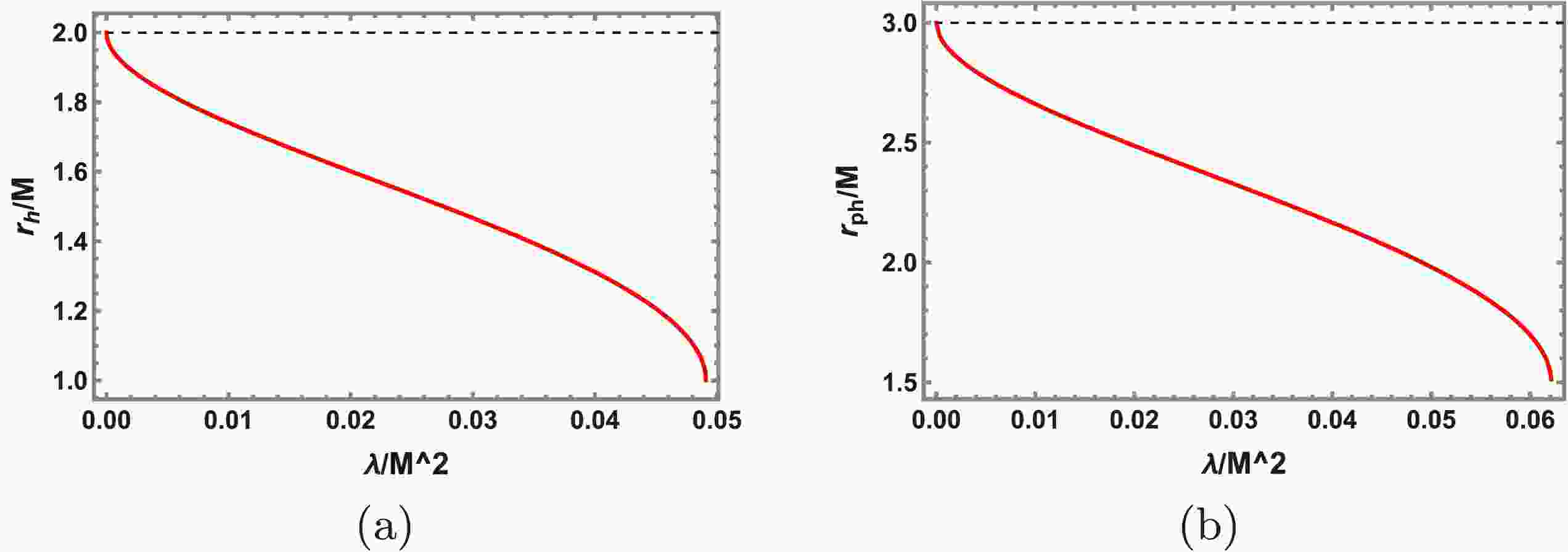
Figure 1 illustrates the influence of spacetime non-commutativity on the characteristic length scales of the black hole. Panel (a) shows the variation of the dimensionless event horizon radius
$ r_h/M $ with the non-commutative parameter$ \lambda/M^2 $ , while panel (b) shows the behavior of the photon sphere radius$ r_{\mathrm{ph}}/M $ . As$ \lambda/M^2 $ increases from zero, both the event horizon radius and the photon sphere radius decrease monotonically. The critical impact parameter$ b_c/M $ , which determines the size of the black hole shadow, exhibits a similar decreasing behavior. This phenomenon indicates that the non-commutative geometric correction reduces the macroscopic observable features of the black hole, such as the shadow diameter.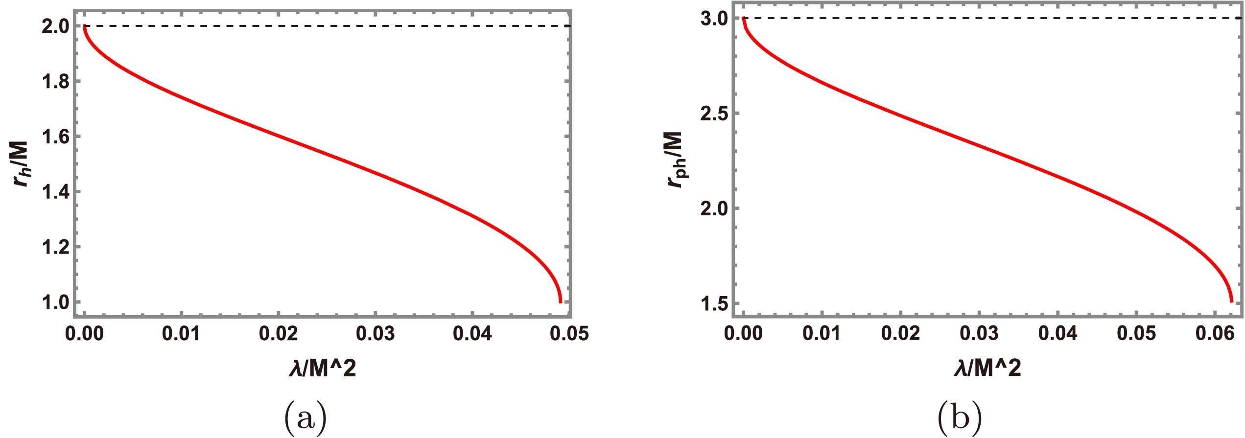
Figure 1. (color online) Variation of the characteristic quantities of the non-commutative Schwarzschild black hole with respect to the non-commutative parameter
$ \lambda/M^2 $ : (a) event horizon radius$ r_{h}/M $ ; (b) photon sphere radius$ r_{\mathrm{ph}}/M $ . In the figures, the solid red line corresponds to the non-commutative black hole, and the dashed black line represents the classical Schwarzschild black hole$ (\lambda=0) $ . -
The Schwarzschild metric describes the geometry of a static, spherically symmetric vacuum spacetime. Its line element is given by
$ {\rm d}s^2 = -A(r){\rm d}t^2 + \frac{1}{A(r)}{\rm d}r^2 + r^2\left({\rm d}\theta^2 + \sin^2\theta {\rm d}\varphi^2\right). $
(1) The classical Schwarzschild metric inevitably contains an intrinsic curvature singularity at
$ r=0 $ . To resolve this central singularity, we adopt the framework of spacetime non-commutativity [21, 22], in which the coordinates satisfy the non-commutative algebra$ [x^\mu, x^\nu] = {\rm i}\lambda^{\mu\nu}, $
(2) $ [x^\mu, x^\nu] = {\rm i}\lambda^{\mu\nu}, $
(3) where
$ \lambda^{\mu\nu} $ is an antisymmetric tensor that introduces a microscopic length scale to mitigate the singularity problem. We employ a Lorentzian-smeared energy density [32]$ \rho_{\lambda}(r) = \dfrac{\sqrt{\lambda} M}{\pi^{3 / 2}\left(r^{2} + \pi \lambda\right)^{2}}. $
(4) This distribution has a finite value at
$ r=0 $ , given by$ \rho_{\lambda}(0)= \dfrac{M}{\pi^{7/2}\lambda^{3/2}} $ . Consequently, the energy density remains finite, thereby eliminating the central spacetime singularity within the effective theoretical framework.Solving the Einstein field equations yields the metric function in the form
$ A(r) = 1 - \frac{2\mathcal{M}_{\lambda}(r)}{r}, $
(5) where the mass accumulation function is
$\begin{aligned}[b] \mathcal{M}_{\lambda}(r)=\;&\int_{0}^{r} \rho_{\lambda}\left(r^{\prime}\right) 4 \pi r^{\prime 2} {\rm d} r^{\prime}\\=\;&\frac{2 M}{\pi}\left(\tan ^{-1}\left(\frac{r}{\sqrt{\pi \lambda}}\right)-\frac{r \sqrt{\pi \lambda}}{r^{2}+\pi \lambda}\right)\\=\;& M - \frac{4\sqrt{\lambda} M}{\sqrt{\pi} r} + \mathcal{O}\left(\lambda^{3/2}\right).\end{aligned} $
(6) In the limit
$ \lambda \to 0 $ , the metric reduces to the classical Schwarzschild solution. Expanding this exact solution in the small-λ approximation (i.e.,$ \sqrt{\lambda} \ll M $ ), we obtain the leading-order correction to the metric function$ A(r) = 1 - \frac{2M}{r} + \frac{8\sqrt{\lambda}M}{\sqrt{\pi}r^2} + \mathcal{O}(\lambda^{3/2}). $
(7) Before deriving the causal structure and photon geodesics from Eq. (7), it is essential to clarify the physical meaning and scaling of the parameter λ. Although λ originally arises from a microscopic spacetime algebra whose natural cutoff scale is associated with the Planck length (
$ \lambda \sim \ell_P^2 $ ) [22], the resulting dimensionless ratio$ \lambda/M^2 $ for astrophysical black holes is suppressed by many orders of magnitude. Because such microscopic scales are fundamentally undetectable by current or foreseeable VLBI networks, we do not treat λ as a direct probe of Planckian quantum gravity in the context of astronomical imaging.Within classical general relativity, the regular spacetime approximated by Eq. (7) is sourced by an anisotropic fluid with a Lorentzian energy density distribution [25, 32]. In this framework, the parameter λ effectively acts as the characteristic macroscopic scale of the regularized fluid core (
$ \lambda/M^2 \sim \mathcal{O}(0.01) $ ).Furthermore, we adopt the standard methodology established in studies of regular black holes. In the literature on nonsingular spacetimes, such as Bardeen or Hayward black holes, regularization parameters are routinely promoted to macroscopic values to test observational constraints [15]. Following this established practice, we use our leading-order metric as an analytically tractable benchmark. This macroscopic interpretation justifies treating λ as a free parameter of order
$ \mathcal{O}\left(10^{-2}\right) M^2 $ in our subsequent derivations [35, 50].Solving the horizon equation
$ A(r) = 0 $ with the expanded metric given by Eq. (7) yields analytical expressions for the radii of the event horizon$ r_+ $ and the Cauchy horizon$ r_- $ ,$ r_{\pm} = M \left( 1 \pm \sqrt{1 - \frac{8\sqrt{\lambda}}{M\sqrt{\pi}}} \right). $
(8) The extremal condition corresponds to the merger of the two horizons (
$ r_+ = r_- $ ). This condition analytically yields the extremal horizon radius$ r_{\text{ext}} = M $ and the critical parameter$ \lambda_c = \pi M^2 / 64 \approx 0.049 M^2 $ . Within this approximation, the value of λ uniquely determines the causal structure of the spacetime. For$ \lambda \lt \lambda_c $ , the metric admits two distinct horizons and describes a regular black hole. For$ \lambda = \lambda_c $ , it describes an extremal regular black hole with a degenerate horizon. Finally, for$ \lambda \gt \lambda_c $ , no horizon exists.Having established the causal structure, we now examine its dynamical properties. From the line element, we can derive the geodesic equations governing photon motion, which then allow us to analyze the optical characteristics of photon orbits through the effective potential. To study photon motion near the black hole, we introduce the Lagrangian formalism. Photon motion is described by the Euler-Lagrange equation
$ \frac{{\rm d}}{{\rm d}\varsigma}\left(\frac{\partial \mathcal{L}}{\partial \dot{x}^{\mu}}\right) = \frac{\partial \mathcal{L}}{\partial x^{\mu}}. $
(9) Here,
$\dot{x}^{\mu} = {\rm d}x^{\mu}/{\rm d}\varsigma$ is the photon's four-velocity, and ς is the affine parameter. For a static, spherically symmetric spacetime, the photon Lagrangian$ \mathcal{L} $ can be written as$ \mathcal{L} = \frac{1}{2}g_{\mu\nu}\dot{x}^{\mu}\dot{x}^{\nu} = \frac{1}{2}\left[ -A(r)\dot{t}^{2} + \frac{1}{A(r)}\dot{r}^{2} + r^{2}\left(\dot{\theta}^{2} + \sin^{2}\theta \dot{\varphi}^{2}\right) \right]. $
(10) Because the metric coefficients are independent of the time coordinate t and the azimuthal angle φ, there exist two Killing vectors,
$ \boldsymbol{\xi}=\partial_t $ and$ \boldsymbol{\psi}=\partial_{\varphi} $ , which correspond to the conserved energy E and angular momentum L, respectively$ E = -g_{tt}\dot{t} = A(r)\frac{{\rm d} t}{{\rm d}\varsigma}, \quad L = g_{\varphi\varphi}\dot{\varphi} = r^{2}\sin ^{2}\theta\frac{{\rm d}\varphi}{{\rm d}\varsigma}. $
(11) For photon motion confined to the equatorial plane (
$ \theta=\pi/2 $ ,$ \dot{\theta}=0 $ ), the angular momentum equation simplifies to$ \frac{{\rm d}\varphi}{{\rm d}\varsigma} = \frac{L}{r^{2}}. $
(12) Since photons travel along null geodesics, they satisfy
$ {\rm d} s^{2} = 0 $ (i.e.,$ 2\mathcal{L}=0 $ ). Substituting the metric components gives$ -A(r)\left(\frac{{\rm d} t}{{\rm d}\varsigma}\right)^{2} + \frac{1}{A(r)}\left(\frac{{\rm d} r}{{\rm d}\varsigma}\right)^{2} + r^{2}\left(\frac{{\rm d}\varphi}{{\rm d}\varsigma}\right)^{2} = 0. $
(13) Substituting the conserved quantities E and L into the equation above and rearranging yields the radial equation of motion for photons
$ \left(\frac{{\rm d}r}{{\rm d}\varsigma}\right)^{2}=E^{2}-\frac{A(r)L^{2}}{r^{2}} . $
(14) To obtain a more intuitive understanding of the orbital motion, we rewrite the radial equation in terms of an effective potential. The effective potential for photons is defined as
$ V_{\text{eff}}(r)=\frac{A(r)L^{2}}{r^{2}}=\frac{L^{2}}{r^{2}}\left(1-\frac{2\mathcal{M}_{\lambda}(r)}{r}\right). $
(15) Eq. (14) can then be rewritten as
$ \left(\frac{{\rm d}r}{{\rm d}\varsigma}\right)^{2}=E^{2}-V_{\text{eff}}(r). $
(16) By introducing the variable
$ u=1/r $ , we derive the orbit equation$ \frac{{\rm d}r}{{\rm d}\varsigma}= -L \frac{{\rm d}u}{{\rm d}\varphi}. $
(17) Substituting this expression into Eq. (14) yields
$ \left(\frac{{\rm d}u}{{\rm d}\varphi}\right)^{2} = \frac{1}{b^{2}} - u^{2}A(1/u), $
(18) where
$ b=L/E $ is the impact parameter. This equation determines the geometric shape of the photon trajectory.Next, we consider the photon sphere associated with unstable circular orbits. Let
$ r_{\rm ph} $ denote the radius of the photon sphere, which must satisfy$ V_{\text{eff}}(r_{\mathrm{ph}}) = E^{2}, \quad \left.\frac{{\rm d} V_{\text{eff}}}{{\rm d} r}\right|_{r=r_{\mathrm{ph}}} = 0. $
(19) From the derivative of the effective potential
$ \frac{{\rm d} V_{\text{eff}}}{{\rm d} r} = L^{2} \frac{{\rm d}}{{\rm d} r}\left(\frac{A(r)}{r^{2}}\right) = L^{2}\left(\frac{A^{\prime}(r)}{r^{2}} - \frac{2 A(r)}{r^{3}}\right), $
(20) the critical condition is given by
$ r A^{\prime}(r) - 2 A(r) = 0. $
(21) Substituting this condition into the metric function
$ A(r) $ and simplifying yields the fundamental equation that the photon sphere radius,$ r = r_{\mathrm{ph}} $ , must satisfy:$ r\mathcal{M}_{\lambda}^{\prime}(r) - 3\mathcal{M}_{\lambda}(r) + r = 0. $
(22) In the limit
$ \lambda \to 0 $ , we have$ \mathcal{M}_{\lambda}(r) \to M $ and$ \mathcal{M}_{\lambda}^{\prime}(r) \to 0 $ . Substituting these limits into Eq. (22) gives$ r_{\mathrm{ph}} = 3M. $
(23) This solution reproduces the photon-sphere radius of the classical Schwarzschild black hole. The critical impact parameter
$ b_{c} $ is$ b_{c} = \frac{r_{\mathrm{ph}}}{\sqrt{A\left(r_{\mathrm{ph}}\right)}}. $
(24) Stability is determined by the second derivative.
$ \left.\frac{{\rm d}^{2} V_{\text{eff}}}{{\rm d} r^{2}}\right|_{r=r_{\mathrm{ph}}} =L^{2}\left.\left(\frac{A^{\prime\prime}(r)}{r^{2}}-\frac{4 A^{\prime}(r)}{r^{3}}+\frac{6 A(r)}{r^{4}}\right)\right|_{r=r_{\mathrm{ph}}}. $
(25) This value is typically negative, indicating an unstable orbit that leads to the formation of photon rings.
Figure 1 illustrates the influence of spacetime non-commutativity on the characteristic length scales of the black hole. Panel (a) shows the variation of the dimensionless event horizon radius
$ r_h/M $ with the non-commutative parameter$ \lambda/M^2 $ , while panel (b) shows the behavior of the photon sphere radius$ r_{\mathrm{ph}}/M $ . As$ \lambda/M^2 $ increases from zero, both the event horizon radius and the photon sphere radius decrease monotonically. The critical impact parameter$ b_c/M $ , which determines the size of the black hole shadow, exhibits a similar decreasing behavior. This phenomenon indicates that the non-commutative geometric correction reduces the macroscopic observable features of the black hole, such as the shadow diameter.
Figure 1. (color online) Variation of the characteristic quantities of the non-commutative Schwarzschild black hole with respect to the non-commutative parameter
$ \lambda/M^2 $ : (a) event horizon radius$ r_{h}/M $ ; (b) photon sphere radius$ r_{\mathrm{ph}}/M $ . In the figures, the solid red line corresponds to the non-commutative black hole, and the dashed black line represents the classical Schwarzschild black hole$ (\lambda=0) $ . -
The Schwarzschild metric describes the geometry of a static, spherically symmetric vacuum spacetime. Its line element is given by
$ {\rm d}s^2 = -A(r){\rm d}t^2 + \frac{1}{A(r)}{\rm d}r^2 + r^2\left({\rm d}\theta^2 + \sin^2\theta {\rm d}\varphi^2\right). $
(1) The classical Schwarzschild metric inevitably contains an intrinsic curvature singularity at
$ r=0 $ . To resolve this central singularity, we adopt the framework of spacetime non-commutativity [21, 22], in which the coordinates satisfy the non-commutative algebra$ [x^\mu, x^\nu] = {\rm i}\lambda^{\mu\nu}, $
(2) $ [x^\mu, x^\nu] = {\rm i}\lambda^{\mu\nu}, $
(3) where
$ \lambda^{\mu\nu} $ is an antisymmetric tensor that introduces a microscopic length scale to mitigate the singularity problem. We employ a Lorentzian-smeared energy density [32]$ \rho_{\lambda}(r) = \dfrac{\sqrt{\lambda} M}{\pi^{3 / 2}\left(r^{2} + \pi \lambda\right)^{2}}. $
(4) This distribution has a finite value at
$ r=0 $ , given by$ \rho_{\lambda}(0)= \dfrac{M}{\pi^{7/2}\lambda^{3/2}} $ . Consequently, the energy density remains finite, thereby eliminating the central spacetime singularity within the effective theoretical framework.Solving the Einstein field equations yields the metric function in the form
$ A(r) = 1 - \frac{2\mathcal{M}_{\lambda}(r)}{r}, $
(5) where the mass accumulation function is
$\begin{aligned}[b] \mathcal{M}_{\lambda}(r)=\;&\int_{0}^{r} \rho_{\lambda}\left(r^{\prime}\right) 4 \pi r^{\prime 2} {\rm d} r^{\prime}\\=\;&\frac{2 M}{\pi}\left(\tan ^{-1}\left(\frac{r}{\sqrt{\pi \lambda}}\right)-\frac{r \sqrt{\pi \lambda}}{r^{2}+\pi \lambda}\right)\\=\;& M - \frac{4\sqrt{\lambda} M}{\sqrt{\pi} r} + \mathcal{O}\left(\lambda^{3/2}\right).\end{aligned} $
(6) In the limit
$ \lambda \to 0 $ , the metric reduces to the classical Schwarzschild solution. Expanding this exact solution in the small-λ approximation (i.e.,$ \sqrt{\lambda} \ll M $ ), we obtain the leading-order correction to the metric function$ A(r) = 1 - \frac{2M}{r} + \frac{8\sqrt{\lambda}M}{\sqrt{\pi}r^2} + \mathcal{O}(\lambda^{3/2}). $
(7) Before deriving the causal structure and photon geodesics from Eq. (7), it is essential to clarify the physical meaning and scaling of the parameter λ. Although λ originally arises from a microscopic spacetime algebra whose natural cutoff scale is associated with the Planck length (
$ \lambda \sim \ell_P^2 $ ) [22], the resulting dimensionless ratio$ \lambda/M^2 $ for astrophysical black holes is suppressed by many orders of magnitude. Because such microscopic scales are fundamentally undetectable by current or foreseeable VLBI networks, we do not treat λ as a direct probe of Planckian quantum gravity in the context of astronomical imaging.Within classical general relativity, the regular spacetime approximated by Eq. (7) is sourced by an anisotropic fluid with a Lorentzian energy density distribution [25, 32]. In this framework, the parameter λ effectively acts as the characteristic macroscopic scale of the regularized fluid core (
$ \lambda/M^2 \sim \mathcal{O}(0.01) $ ).Furthermore, we adopt the standard methodology established in studies of regular black holes. In the literature on nonsingular spacetimes, such as Bardeen or Hayward black holes, regularization parameters are routinely promoted to macroscopic values to test observational constraints [15]. Following this established practice, we use our leading-order metric as an analytically tractable benchmark. This macroscopic interpretation justifies treating λ as a free parameter of order
$ \mathcal{O}\left(10^{-2}\right) M^2 $ in our subsequent derivations [35, 50].Solving the horizon equation
$ A(r) = 0 $ with the expanded metric given by Eq. (7) yields analytical expressions for the radii of the event horizon$ r_+ $ and the Cauchy horizon$ r_- $ ,$ r_{\pm} = M \left( 1 \pm \sqrt{1 - \frac{8\sqrt{\lambda}}{M\sqrt{\pi}}} \right). $
(8) The extremal condition corresponds to the merger of the two horizons (
$ r_+ = r_- $ ). This condition analytically yields the extremal horizon radius$ r_{\text{ext}} = M $ and the critical parameter$ \lambda_c = \pi M^2 / 64 \approx 0.049 M^2 $ . Within this approximation, the value of λ uniquely determines the causal structure of the spacetime. For$ \lambda \lt \lambda_c $ , the metric admits two distinct horizons and describes a regular black hole. For$ \lambda = \lambda_c $ , it describes an extremal regular black hole with a degenerate horizon. Finally, for$ \lambda \gt \lambda_c $ , no horizon exists.Having established the causal structure, we now examine its dynamical properties. From the line element, we can derive the geodesic equations governing photon motion, which then allow us to analyze the optical characteristics of photon orbits through the effective potential. To study photon motion near the black hole, we introduce the Lagrangian formalism. Photon motion is described by the Euler-Lagrange equation
$ \frac{{\rm d}}{{\rm d}\varsigma}\left(\frac{\partial \mathcal{L}}{\partial \dot{x}^{\mu}}\right) = \frac{\partial \mathcal{L}}{\partial x^{\mu}}. $
(9) Here,
$\dot{x}^{\mu} = {\rm d}x^{\mu}/{\rm d}\varsigma$ is the photon's four-velocity, and ς is the affine parameter. For a static, spherically symmetric spacetime, the photon Lagrangian$ \mathcal{L} $ can be written as$ \mathcal{L} = \frac{1}{2}g_{\mu\nu}\dot{x}^{\mu}\dot{x}^{\nu} = \frac{1}{2}\left[ -A(r)\dot{t}^{2} + \frac{1}{A(r)}\dot{r}^{2} + r^{2}\left(\dot{\theta}^{2} + \sin^{2}\theta \dot{\varphi}^{2}\right) \right]. $
(10) Because the metric coefficients are independent of the time coordinate t and the azimuthal angle φ, there exist two Killing vectors,
$ \boldsymbol{\xi}=\partial_t $ and$ \boldsymbol{\psi}=\partial_{\varphi} $ , which correspond to the conserved energy E and angular momentum L, respectively$ E = -g_{tt}\dot{t} = A(r)\frac{{\rm d} t}{{\rm d}\varsigma}, \quad L = g_{\varphi\varphi}\dot{\varphi} = r^{2}\sin ^{2}\theta\frac{{\rm d}\varphi}{{\rm d}\varsigma}. $
(11) For photon motion confined to the equatorial plane (
$ \theta=\pi/2 $ ,$ \dot{\theta}=0 $ ), the angular momentum equation simplifies to$ \frac{{\rm d}\varphi}{{\rm d}\varsigma} = \frac{L}{r^{2}}. $
(12) Since photons travel along null geodesics, they satisfy
$ {\rm d} s^{2} = 0 $ (i.e.,$ 2\mathcal{L}=0 $ ). Substituting the metric components gives$ -A(r)\left(\frac{{\rm d} t}{{\rm d}\varsigma}\right)^{2} + \frac{1}{A(r)}\left(\frac{{\rm d} r}{{\rm d}\varsigma}\right)^{2} + r^{2}\left(\frac{{\rm d}\varphi}{{\rm d}\varsigma}\right)^{2} = 0. $
(13) Substituting the conserved quantities E and L into the equation above and rearranging yields the radial equation of motion for photons
$ \left(\frac{{\rm d}r}{{\rm d}\varsigma}\right)^{2}=E^{2}-\frac{A(r)L^{2}}{r^{2}} . $
(14) To obtain a more intuitive understanding of the orbital motion, we rewrite the radial equation in terms of an effective potential. The effective potential for photons is defined as
$ V_{\text{eff}}(r)=\frac{A(r)L^{2}}{r^{2}}=\frac{L^{2}}{r^{2}}\left(1-\frac{2\mathcal{M}_{\lambda}(r)}{r}\right). $
(15) Eq. (14) can then be rewritten as
$ \left(\frac{{\rm d}r}{{\rm d}\varsigma}\right)^{2}=E^{2}-V_{\text{eff}}(r). $
(16) By introducing the variable
$ u=1/r $ , we derive the orbit equation$ \frac{{\rm d}r}{{\rm d}\varsigma}= -L \frac{{\rm d}u}{{\rm d}\varphi}. $
(17) Substituting this expression into Eq. (14) yields
$ \left(\frac{{\rm d}u}{{\rm d}\varphi}\right)^{2} = \frac{1}{b^{2}} - u^{2}A(1/u), $
(18) where
$ b=L/E $ is the impact parameter. This equation determines the geometric shape of the photon trajectory.Next, we consider the photon sphere associated with unstable circular orbits. Let
$ r_{\rm ph} $ denote the radius of the photon sphere, which must satisfy$ V_{\text{eff}}(r_{\mathrm{ph}}) = E^{2}, \quad \left.\frac{{\rm d} V_{\text{eff}}}{{\rm d} r}\right|_{r=r_{\mathrm{ph}}} = 0. $
(19) From the derivative of the effective potential
$ \frac{{\rm d} V_{\text{eff}}}{{\rm d} r} = L^{2} \frac{{\rm d}}{{\rm d} r}\left(\frac{A(r)}{r^{2}}\right) = L^{2}\left(\frac{A^{\prime}(r)}{r^{2}} - \frac{2 A(r)}{r^{3}}\right), $
(20) the critical condition is given by
$ r A^{\prime}(r) - 2 A(r) = 0. $
(21) Substituting this condition into the metric function
$ A(r) $ and simplifying yields the fundamental equation that the photon sphere radius,$ r = r_{\mathrm{ph}} $ , must satisfy:$ r\mathcal{M}_{\lambda}^{\prime}(r) - 3\mathcal{M}_{\lambda}(r) + r = 0. $
(22) In the limit
$ \lambda \to 0 $ , we have$ \mathcal{M}_{\lambda}(r) \to M $ and$ \mathcal{M}_{\lambda}^{\prime}(r) \to 0 $ . Substituting these limits into Eq. (22) gives$ r_{\mathrm{ph}} = 3M. $
(23) This solution reproduces the photon-sphere radius of the classical Schwarzschild black hole. The critical impact parameter
$ b_{c} $ is$ b_{c} = \frac{r_{\mathrm{ph}}}{\sqrt{A\left(r_{\mathrm{ph}}\right)}}. $
(24) Stability is determined by the second derivative.
$ \left.\frac{{\rm d}^{2} V_{\text{eff}}}{{\rm d} r^{2}}\right|_{r=r_{\mathrm{ph}}} =L^{2}\left.\left(\frac{A^{\prime\prime}(r)}{r^{2}}-\frac{4 A^{\prime}(r)}{r^{3}}+\frac{6 A(r)}{r^{4}}\right)\right|_{r=r_{\mathrm{ph}}}. $
(25) This value is typically negative, indicating an unstable orbit that leads to the formation of photon rings.
Figure 1 illustrates the influence of spacetime non-commutativity on the characteristic length scales of the black hole. Panel (a) shows the variation of the dimensionless event horizon radius
$ r_h/M $ with the non-commutative parameter$ \lambda/M^2 $ , while panel (b) shows the behavior of the photon sphere radius$ r_{\mathrm{ph}}/M $ . As$ \lambda/M^2 $ increases from zero, both the event horizon radius and the photon sphere radius decrease monotonically. The critical impact parameter$ b_c/M $ , which determines the size of the black hole shadow, exhibits a similar decreasing behavior. This phenomenon indicates that the non-commutative geometric correction reduces the macroscopic observable features of the black hole, such as the shadow diameter.
Figure 1. (color online) Variation of the characteristic quantities of the non-commutative Schwarzschild black hole with respect to the non-commutative parameter
$ \lambda/M^2 $ : (a) event horizon radius$ r_{h}/M $ ; (b) photon sphere radius$ r_{\mathrm{ph}}/M $ . In the figures, the solid red line corresponds to the non-commutative black hole, and the dashed black line represents the classical Schwarzschild black hole$ (\lambda=0) $ . -
This section constructs a theoretical framework for describing the radiation processes in black hole accretion flows. We first introduce the covariant radiative transfer equation in curved spacetime. We then focus on the dominant radiation mechanism in the accretion flow, thermal electron synchrotron radiation, and present detailed expressions for its emissivity and absorption coefficient under a relativistic thermal distribution. Finally, we describe the parametric accretion flow model adopted in this paper to simplify the numerical simulations.
-
This section constructs a theoretical framework for describing the radiation processes in black hole accretion flows. We first introduce the covariant radiative transfer equation in curved spacetime. We then focus on the dominant radiation mechanism in the accretion flow, thermal electron synchrotron radiation, and present detailed expressions for its emissivity and absorption coefficient under a relativistic thermal distribution. Finally, we describe the parametric accretion flow model adopted in this paper to simplify the numerical simulations.
-
This section constructs a theoretical framework for describing the radiation processes in black hole accretion flows. We first introduce the covariant radiative transfer equation in curved spacetime. We then focus on the dominant radiation mechanism in the accretion flow, thermal electron synchrotron radiation, and present detailed expressions for its emissivity and absorption coefficient under a relativistic thermal distribution. Finally, we describe the parametric accretion flow model adopted in this paper to simplify the numerical simulations.
-
For optically thin and geometrically thick radiation sources, such as thick accretion disks, solving for the radiation field requires a radiative transfer theory formulated within the framework of general relativity. In this context, using Lorentz invariants that are consistent with the spacetime geometry as conserved quantities is essential for describing photon propagation and radiation evolution in strong gravitational fields.
Along a photon trajectory, the evolution of the radiation field is governed by the covariant form of the general relativistic radiative transfer equation. Expressed in terms of the affine parameter ς, the differential equation is [51, 52]
$ \frac{{\rm d}d}{{\rm d}\varsigma} \tilde{I} = \tilde{J} - \tilde{\alpha} \tilde{I}. $
(26) Here,
$ \tilde{I} $ ,$ \tilde{J} $ , and$ \tilde{\alpha} $ are general-relativistic invariants related to the physical quantities$ I_{\nu} $ ,$ j_{\nu} $ , and$ \alpha_{\nu} $ in the local reference frame by$ \tilde{I} = \frac{I_{\nu}}{\nu^{3}}, \quad \tilde{J} = \frac{j_{\nu}}{\nu^{2}}, \quad \tilde{\alpha} = \nu \alpha_{\nu}. $
(27) In the isotropic emission model, the emission coefficient
$ j_{\nu} $ that enters the radiative transfer equation is taken to be the angle-averaged quantity$ \hat{j}_{\nu} $ defined in Sec. IV; in the anisotropic model, the explicitly pitch-angle-dependent$ j_{\nu}(\theta_b) $ is used instead. The formal solution of Eq. (26) is given by$ \begin{aligned}[b]\tilde I(\varsigma)=\;&\tilde I(\varsigma_0)\exp \left[- \int_{\varsigma_0}^{\varsigma} \tilde\alpha(\varsigma')\,{\rm d}\varsigma'\right] \\& + \int_{\varsigma_0}^{\varsigma} \tilde J(\varsigma')\,\exp \left[- \int_{\varsigma'}^{\varsigma} \tilde\alpha(\varsigma'')\,{\rm d}\varsigma''\right] {\rm d}\varsigma' .\end{aligned} $
(28) To express the formulation in the CGS unit system, a scaling factor
$ C = r_{g}/\nu_{0} $ must be introduced, where$ r_{g} = GM/c^{2} $ is the gravitational radius and$ \nu_0 $ is the reference photon frequency at the observer's location. After this transformation, the radiative transfer equation and its solution can be rewritten in a practical form that incorporates the redshift factor$ g = \nu_{\rm obs}/\nu_{\rm em} $ ,$ \begin{aligned}[b]I_{\nu} =\;& g^{3} I_{\nu_0} + r_g \int_{\varsigma_0}^{\varsigma} g^{3}(\varsigma')\, j_\nu(\varsigma')\,\\&\times \exp \left[-\, r_g \int_{\varsigma'}^{\varsigma} g(\varsigma'')\, \alpha_\nu(\varsigma'')\, d\varsigma" \right] {\rm d}\varsigma' .\end{aligned} $
(29) In this formulation, both
$ I_{\nu} $ and$ I_{\nu_{0}} $ refer to measurements made by the observer. The quantities$ j_{\nu} $ and$ \alpha_{\nu} $ in the integrand are the emission and absorption coefficients, respectively, evaluated in the local rest frame of the fluid. They correspond to the local frequency$ \nu_{\text{em}} $ in that frame. The redshift factor g is determined jointly by the relative motion between the observer and the emitting source and by the difference in gravitational potential. If the fluid four-velocity is$ u^{\mu} $ and the photon four-momentum is$ k_{\mu} $ , with the convention that$ k_{t} = -1 $ in the frame of a stationary observer at infinity, then the redshift factor can be calculated as [53]$ g \equiv \frac{\nu_{\text{obs}}}{\nu_{\text{em}}}=\frac{u^\mu_{\text{obs}}k_\mu}{u^\mu k_\mu} = -\,\frac{1}{k_\mu u^\mu}\, . $
(30) -
For optically thin and geometrically thick radiation sources, such as thick accretion disks, solving for the radiation field requires a radiative transfer theory formulated within the framework of general relativity. In this context, using Lorentz invariants that are consistent with the spacetime geometry as conserved quantities is essential for describing photon propagation and radiation evolution in strong gravitational fields.
Along a photon trajectory, the evolution of the radiation field is governed by the covariant form of the general relativistic radiative transfer equation. Expressed in terms of the affine parameter ς, the differential equation is [51, 52]
$ \frac{{\rm d}d}{{\rm d}\varsigma} \tilde{I} = \tilde{J} - \tilde{\alpha} \tilde{I}. $
(26) Here,
$ \tilde{I} $ ,$ \tilde{J} $ , and$ \tilde{\alpha} $ are general-relativistic invariants related to the physical quantities$ I_{\nu} $ ,$ j_{\nu} $ , and$ \alpha_{\nu} $ in the local reference frame by$ \tilde{I} = \frac{I_{\nu}}{\nu^{3}}, \quad \tilde{J} = \frac{j_{\nu}}{\nu^{2}}, \quad \tilde{\alpha} = \nu \alpha_{\nu}. $
(27) In the isotropic emission model, the emission coefficient
$ j_{\nu} $ that enters the radiative transfer equation is taken to be the angle-averaged quantity$ \hat{j}_{\nu} $ defined in Sec. IV; in the anisotropic model, the explicitly pitch-angle-dependent$ j_{\nu}(\theta_b) $ is used instead. The formal solution of Eq. (26) is given by$ \begin{aligned}[b]\tilde I(\varsigma)=\;&\tilde I(\varsigma_0)\exp \left[- \int_{\varsigma_0}^{\varsigma} \tilde\alpha(\varsigma')\,{\rm d}\varsigma'\right] \\& + \int_{\varsigma_0}^{\varsigma} \tilde J(\varsigma')\,\exp \left[- \int_{\varsigma'}^{\varsigma} \tilde\alpha(\varsigma'')\,{\rm d}\varsigma''\right] {\rm d}\varsigma' .\end{aligned} $
(28) To express the formulation in the CGS unit system, a scaling factor
$ C = r_{g}/\nu_{0} $ must be introduced, where$ r_{g} = GM/c^{2} $ is the gravitational radius and$ \nu_0 $ is the reference photon frequency at the observer's location. After this transformation, the radiative transfer equation and its solution can be rewritten in a practical form that incorporates the redshift factor$ g = \nu_{\rm obs}/\nu_{\rm em} $ ,$ \begin{aligned}[b]I_{\nu} =\;& g^{3} I_{\nu_0} + r_g \int_{\varsigma_0}^{\varsigma} g^{3}(\varsigma')\, j_\nu(\varsigma')\,\\&\times \exp \left[-\, r_g \int_{\varsigma'}^{\varsigma} g(\varsigma'')\, \alpha_\nu(\varsigma'')\, d\varsigma" \right] {\rm d}\varsigma' .\end{aligned} $
(29) In this formulation, both
$ I_{\nu} $ and$ I_{\nu_{0}} $ refer to measurements made by the observer. The quantities$ j_{\nu} $ and$ \alpha_{\nu} $ in the integrand are the emission and absorption coefficients, respectively, evaluated in the local rest frame of the fluid. They correspond to the local frequency$ \nu_{\text{em}} $ in that frame. The redshift factor g is determined jointly by the relative motion between the observer and the emitting source and by the difference in gravitational potential. If the fluid four-velocity is$ u^{\mu} $ and the photon four-momentum is$ k_{\mu} $ , with the convention that$ k_{t} = -1 $ in the frame of a stationary observer at infinity, then the redshift factor can be calculated as [53]$ g \equiv \frac{\nu_{\text{obs}}}{\nu_{\text{em}}}=\frac{u^\mu_{\text{obs}}k_\mu}{u^\mu k_\mu} = -\,\frac{1}{k_\mu u^\mu}\, . $
(30) -
For optically thin and geometrically thick radiation sources, such as thick accretion disks, solving for the radiation field requires a radiative transfer theory formulated within the framework of general relativity. In this context, using Lorentz invariants that are consistent with the spacetime geometry as conserved quantities is essential for describing photon propagation and radiation evolution in strong gravitational fields.
Along a photon trajectory, the evolution of the radiation field is governed by the covariant form of the general relativistic radiative transfer equation. Expressed in terms of the affine parameter ς, the differential equation is [51, 52]
$ \frac{{\rm d}d}{{\rm d}\varsigma} \tilde{I} = \tilde{J} - \tilde{\alpha} \tilde{I}. $
(26) Here,
$ \tilde{I} $ ,$ \tilde{J} $ , and$ \tilde{\alpha} $ are general-relativistic invariants related to the physical quantities$ I_{\nu} $ ,$ j_{\nu} $ , and$ \alpha_{\nu} $ in the local reference frame by$ \tilde{I} = \frac{I_{\nu}}{\nu^{3}}, \quad \tilde{J} = \frac{j_{\nu}}{\nu^{2}}, \quad \tilde{\alpha} = \nu \alpha_{\nu}. $
(27) In the isotropic emission model, the emission coefficient
$ j_{\nu} $ that enters the radiative transfer equation is taken to be the angle-averaged quantity$ \hat{j}_{\nu} $ defined in Sec. IV; in the anisotropic model, the explicitly pitch-angle-dependent$ j_{\nu}(\theta_b) $ is used instead. The formal solution of Eq. (26) is given by$ \begin{aligned}[b]\tilde I(\varsigma)=\;&\tilde I(\varsigma_0)\exp \left[- \int_{\varsigma_0}^{\varsigma} \tilde\alpha(\varsigma')\,{\rm d}\varsigma'\right] \\& + \int_{\varsigma_0}^{\varsigma} \tilde J(\varsigma')\,\exp \left[- \int_{\varsigma'}^{\varsigma} \tilde\alpha(\varsigma'')\,{\rm d}\varsigma''\right] {\rm d}\varsigma' .\end{aligned} $
(28) To express the formulation in the CGS unit system, a scaling factor
$ C = r_{g}/\nu_{0} $ must be introduced, where$ r_{g} = GM/c^{2} $ is the gravitational radius and$ \nu_0 $ is the reference photon frequency at the observer's location. After this transformation, the radiative transfer equation and its solution can be rewritten in a practical form that incorporates the redshift factor$ g = \nu_{\rm obs}/\nu_{\rm em} $ ,$ \begin{aligned}[b]I_{\nu} =\;& g^{3} I_{\nu_0} + r_g \int_{\varsigma_0}^{\varsigma} g^{3}(\varsigma')\, j_\nu(\varsigma')\,\\&\times \exp \left[-\, r_g \int_{\varsigma'}^{\varsigma} g(\varsigma'')\, \alpha_\nu(\varsigma'')\, d\varsigma" \right] {\rm d}\varsigma' .\end{aligned} $
(29) In this formulation, both
$ I_{\nu} $ and$ I_{\nu_{0}} $ refer to measurements made by the observer. The quantities$ j_{\nu} $ and$ \alpha_{\nu} $ in the integrand are the emission and absorption coefficients, respectively, evaluated in the local rest frame of the fluid. They correspond to the local frequency$ \nu_{\text{em}} $ in that frame. The redshift factor g is determined jointly by the relative motion between the observer and the emitting source and by the difference in gravitational potential. If the fluid four-velocity is$ u^{\mu} $ and the photon four-momentum is$ k_{\mu} $ , with the convention that$ k_{t} = -1 $ in the frame of a stationary observer at infinity, then the redshift factor can be calculated as [53]$ g \equiv \frac{\nu_{\text{obs}}}{\nu_{\text{em}}}=\frac{u^\mu_{\text{obs}}k_\mu}{u^\mu k_\mu} = -\,\frac{1}{k_\mu u^\mu}\, . $
(30) -
In this section, we present the explicit forms of the emission coefficient
$ j_\nu $ and the absorption coefficient$ \alpha_\nu $ for the synchrotron radiation mechanism. We consider synchrotron radiation from electrons in a magnetic field under ultra-relativistic conditions. The CGS unit system is adopted. The basic physical constants used in this section are the elementary charge e, the electron mass$ m_e $ , the speed of light c, the Planck constant h, and the Boltzmann constant$ k_B $ .In a plasma environment, synchrotron radiation originates predominantly from electrons. Its emissivity is given by the following integral expression [54]
$ j_{\nu} = \frac{\sqrt{3} e^{3} B \sin\theta_{b}}{4\pi m_{e} c^{2}} \int_{0}^{\infty} {\rm d}\gamma \, \mathcal{N}(\gamma) F\left(\frac{\nu}{\nu_{s}}\right). $
(31) This expression plays an important role in studies of imaging thick accretion disks. Here,
$ \gamma = 1 / \sqrt{1 - \beta^{2}} $ is the Lorentz factor of the charged particle, and$ \mathcal{N}(\gamma) $ is the energy distribution function. The function$ F(x) $ is defined as [54]$ F(x) = x \int_{x}^{\infty} {\rm d}y \, K_{5/3}(y). $
(32) Here,
$ K_{n}(x) $ denotes the modified Bessel function of the second kind of order n. The angle$ \theta_{b} $ is defined between the unit vectors$ e_{(b)}^{\mu} $ and$ e_{(k)}^{\mu} $ and is calculated as$ \theta_{b} = \arccos\left(e_{(b)}^{\mu} \cdot e_{(k)}^{\mu}\right) = \arccos\left[\frac{g}{b}\left(b_{\mu} k^{\mu}\right)\right]. $
(33) The unit vectors are defined as:
$ e_{(k)}^{\mu} = -\left(\frac{k^{\mu}}{u^{\nu} k_{\nu}} + u^{\mu}\right), \quad e_{(b)}^{\mu} = \frac{b^{\mu}}{b}. $
(34) In this expression, B denotes the local magnetic-field strength. The characteristic synchrotron frequency is defined as [46, 55]
$ \nu_{s} = \frac{3 e B \sin \theta_{b} \gamma^{2}}{4 \pi m_{e} c}. $
(35) For an electron system in thermal equilibrium, the energy distribution function is
$ \mathcal{N}(\gamma) = \frac{n_{e} \gamma^{2} \beta}{\Theta_{e} K_{2}(1/\Theta_{e})} {\rm e}^{(-\gamma/\Theta_{e})}, $
(36) where
$ n_{e} $ is the electron number density. The quantity$ \Theta_{e} = \dfrac{k_{B} T_{e}}{m_{e} c^{2}} $ is the dimensionless electron temperature, and$ T_{e} $ is the thermodynamic temperature of the electrons.In the ultrarelativistic limit, where
$ (\beta \approx 1, \Theta_{e} \gg 1) $ , the asymptotic relation$ K_{2}\left(1/\Theta_{e}\right) \approx 2\Theta_{e}^{2} $ can be applied. Introducing the variable substitution$ z = \gamma / \Theta_{e} $ , the emissivity can be simplified as [55, 56]$ j_{\nu} = \frac{\sqrt{3}n_{e} {e}^{3}B\sin\theta_{b}}{8\pi m_{e}c^{2}} \int_{0}^{\infty} {\rm d}z\, z^{2} {\rm e}^{-z} F\left(\frac{\nu}{\nu_{s}}\right). $
(37) Furthermore, by introducing the dimensionless frequency
$ x = \nu / \nu_c $ , we obtain$ \nu / \nu_s = x / z^2 $ . The final expression for the emissivity is therefore given by$ j_{\nu} = \frac{n_{e} e^{2} \nu}{2\sqrt{3}c\Theta_{e}^{2}} \mathcal{F}(x), \quad x = \frac{\nu}{\nu_{c}}, \quad \nu_{c} = \frac{3eB\sin\theta_{b}\Theta_{e}^{2}}{4\pi m_{e}c}. $
(38) The dimensionless function is defined as follows [55]
$ \mathcal{F}(x) = \frac{1}{x} \int_{0}^{\infty} z^{2} {\rm e}^{-z} F\left(\frac{x}{z^{2}}\right) {\rm d}z. $
(39) In the context of a thermal electron distribution, the absorption coefficient
$ \alpha_{\nu} $ can be obtained from Kirchhoff's law [54]$ \alpha_{\nu} = \frac{j_{\nu}}{B_{\nu}}, \quad B_{\nu} = \frac{2 h\nu^{3}}{c^{2}} \frac{1}{\exp\left(h\nu /k_{B}T_{e}\right)-1}. $
(40) Here,
$ B_{\nu} $ denotes the Planck blackbody radiation function.To facilitate numerical computations, the following normalization constants are defined [46, 57]:
$\begin{aligned}[b]& \zeta_{1} = \frac{n_{h} e^{2} \nu_{h}}{2 \sqrt{3} c \Theta_{h}^{2}}, \quad \zeta_{2} = \frac{4 \pi}{3} \frac{m_{e} c \nu_{h}}{e b_{h} \Theta_{h}^{2}}, \\& \zeta_{3} = \frac{h \nu_{h}}{m_{e} c^{2}} \frac{1}{\Theta_{h}}, \quad \zeta_{4} = \frac{2 h \nu_{h}^{3}}{c^{2}}, \quad \zeta_{5} = \left(n_{h} m_{p} c^{2}\right)^{\frac{1}{2}}. \end{aligned}$
(41) Here,
$ n_{h} $ and$ \Theta_{h} $ denote the reference values evaluated at the event horizon. The characteristic frequency is$ \nu_{h} = 10^{9}\,\mathrm{Hz} = 1\,\mathrm{GHz} $ , and the characteristic magnetic field is$ b_{h} = 1\,\mathrm{G} $ . Within this parameterization framework, the radiative quantities can be expressed as$ \hat{j}_{\nu} = \zeta_{1} \bar{n}_{e} \bar{\nu} \tilde{\Theta}_{e}^{-2} \mathcal{F}(x), \;\;\; x = \frac{\zeta_{2} \bar{\nu}}{\bar{b} \sin\theta_{b} \tilde{\Theta}_{e}^{2}}, \;\;\; B_{\nu} = \frac{\zeta_{4} \bar{\nu}^{3}}{\exp\left(\zeta_{3} \bar{\nu} / \tilde{\Theta}_{e}\right) - 1}. $
(42) The normalized variables are defined explicitly as
$ \bar{\nu} = \frac{\nu}{\nu_{h}}, \quad \bar{n}_{e} = \frac{n_{e}}{n_{h}}, \quad \bar{b} = \frac{B}{b_{h}}, \quad \tilde{\Theta}_{e} = \frac{\Theta_{e}}{\Theta_{h}}. $
(43) Using Eqs. (39) and (42), the radiative transfer equation, Eq. (26), can in principle be solved to obtain the radiation intensity. The specific forms of the electron number density, electron temperature, and dimensionless function
$ \mathcal{F}(x) $ are specified in Sec. IV together with the accretion disk model. -
In this section, we present the explicit forms of the emission coefficient
$ j_\nu $ and the absorption coefficient$ \alpha_\nu $ for the synchrotron radiation mechanism. We consider synchrotron radiation from electrons in a magnetic field under ultra-relativistic conditions. The CGS unit system is adopted. The basic physical constants used in this section are the elementary charge e, the electron mass$ m_e $ , the speed of light c, the Planck constant h, and the Boltzmann constant$ k_B $ .In a plasma environment, synchrotron radiation originates predominantly from electrons. Its emissivity is given by the following integral expression [54]
$ j_{\nu} = \frac{\sqrt{3} e^{3} B \sin\theta_{b}}{4\pi m_{e} c^{2}} \int_{0}^{\infty} {\rm d}\gamma \, \mathcal{N}(\gamma) F\left(\frac{\nu}{\nu_{s}}\right). $
(31) This expression plays an important role in studies of imaging thick accretion disks. Here,
$ \gamma = 1 / \sqrt{1 - \beta^{2}} $ is the Lorentz factor of the charged particle, and$ \mathcal{N}(\gamma) $ is the energy distribution function. The function$ F(x) $ is defined as [54]$ F(x) = x \int_{x}^{\infty} {\rm d}y \, K_{5/3}(y). $
(32) Here,
$ K_{n}(x) $ denotes the modified Bessel function of the second kind of order n. The angle$ \theta_{b} $ is defined between the unit vectors$ e_{(b)}^{\mu} $ and$ e_{(k)}^{\mu} $ and is calculated as$ \theta_{b} = \arccos\left(e_{(b)}^{\mu} \cdot e_{(k)}^{\mu}\right) = \arccos\left[\frac{g}{b}\left(b_{\mu} k^{\mu}\right)\right]. $
(33) The unit vectors are defined as:
$ e_{(k)}^{\mu} = -\left(\frac{k^{\mu}}{u^{\nu} k_{\nu}} + u^{\mu}\right), \quad e_{(b)}^{\mu} = \frac{b^{\mu}}{b}. $
(34) In this expression, B denotes the local magnetic-field strength. The characteristic synchrotron frequency is defined as [46, 55]
$ \nu_{s} = \frac{3 e B \sin \theta_{b} \gamma^{2}}{4 \pi m_{e} c}. $
(35) For an electron system in thermal equilibrium, the energy distribution function is
$ \mathcal{N}(\gamma) = \frac{n_{e} \gamma^{2} \beta}{\Theta_{e} K_{2}(1/\Theta_{e})} {\rm e}^{(-\gamma/\Theta_{e})}, $
(36) where
$ n_{e} $ is the electron number density. The quantity$ \Theta_{e} = \dfrac{k_{B} T_{e}}{m_{e} c^{2}} $ is the dimensionless electron temperature, and$ T_{e} $ is the thermodynamic temperature of the electrons.In the ultrarelativistic limit, where
$ (\beta \approx 1, \Theta_{e} \gg 1) $ , the asymptotic relation$ K_{2}\left(1/\Theta_{e}\right) \approx 2\Theta_{e}^{2} $ can be applied. Introducing the variable substitution$ z = \gamma / \Theta_{e} $ , the emissivity can be simplified as [55, 56]$ j_{\nu} = \frac{\sqrt{3}n_{e} {e}^{3}B\sin\theta_{b}}{8\pi m_{e}c^{2}} \int_{0}^{\infty} {\rm d}z\, z^{2} {\rm e}^{-z} F\left(\frac{\nu}{\nu_{s}}\right). $
(37) Furthermore, by introducing the dimensionless frequency
$ x = \nu / \nu_c $ , we obtain$ \nu / \nu_s = x / z^2 $ . The final expression for the emissivity is therefore given by$ j_{\nu} = \frac{n_{e} e^{2} \nu}{2\sqrt{3}c\Theta_{e}^{2}} \mathcal{F}(x), \quad x = \frac{\nu}{\nu_{c}}, \quad \nu_{c} = \frac{3eB\sin\theta_{b}\Theta_{e}^{2}}{4\pi m_{e}c}. $
(38) The dimensionless function is defined as follows [55]
$ \mathcal{F}(x) = \frac{1}{x} \int_{0}^{\infty} z^{2} {\rm e}^{-z} F\left(\frac{x}{z^{2}}\right) {\rm d}z. $
(39) In the context of a thermal electron distribution, the absorption coefficient
$ \alpha_{\nu} $ can be obtained from Kirchhoff's law [54]$ \alpha_{\nu} = \frac{j_{\nu}}{B_{\nu}}, \quad B_{\nu} = \frac{2 h\nu^{3}}{c^{2}} \frac{1}{\exp\left(h\nu /k_{B}T_{e}\right)-1}. $
(40) Here,
$ B_{\nu} $ denotes the Planck blackbody radiation function.To facilitate numerical computations, the following normalization constants are defined [46, 57]:
$\begin{aligned}[b]& \zeta_{1} = \frac{n_{h} e^{2} \nu_{h}}{2 \sqrt{3} c \Theta_{h}^{2}}, \quad \zeta_{2} = \frac{4 \pi}{3} \frac{m_{e} c \nu_{h}}{e b_{h} \Theta_{h}^{2}}, \\& \zeta_{3} = \frac{h \nu_{h}}{m_{e} c^{2}} \frac{1}{\Theta_{h}}, \quad \zeta_{4} = \frac{2 h \nu_{h}^{3}}{c^{2}}, \quad \zeta_{5} = \left(n_{h} m_{p} c^{2}\right)^{\frac{1}{2}}. \end{aligned}$
(41) Here,
$ n_{h} $ and$ \Theta_{h} $ denote the reference values evaluated at the event horizon. The characteristic frequency is$ \nu_{h} = 10^{9}\,\mathrm{Hz} = 1\,\mathrm{GHz} $ , and the characteristic magnetic field is$ b_{h} = 1\,\mathrm{G} $ . Within this parameterization framework, the radiative quantities can be expressed as$ \hat{j}_{\nu} = \zeta_{1} \bar{n}_{e} \bar{\nu} \tilde{\Theta}_{e}^{-2} \mathcal{F}(x), \;\;\; x = \frac{\zeta_{2} \bar{\nu}}{\bar{b} \sin\theta_{b} \tilde{\Theta}_{e}^{2}}, \;\;\; B_{\nu} = \frac{\zeta_{4} \bar{\nu}^{3}}{\exp\left(\zeta_{3} \bar{\nu} / \tilde{\Theta}_{e}\right) - 1}. $
(42) The normalized variables are defined explicitly as
$ \bar{\nu} = \frac{\nu}{\nu_{h}}, \quad \bar{n}_{e} = \frac{n_{e}}{n_{h}}, \quad \bar{b} = \frac{B}{b_{h}}, \quad \tilde{\Theta}_{e} = \frac{\Theta_{e}}{\Theta_{h}}. $
(43) Using Eqs. (39) and (42), the radiative transfer equation, Eq. (26), can in principle be solved to obtain the radiation intensity. The specific forms of the electron number density, electron temperature, and dimensionless function
$ \mathcal{F}(x) $ are specified in Sec. IV together with the accretion disk model. -
In this section, we present the explicit forms of the emission coefficient
$ j_\nu $ and the absorption coefficient$ \alpha_\nu $ for the synchrotron radiation mechanism. We consider synchrotron radiation from electrons in a magnetic field under ultra-relativistic conditions. The CGS unit system is adopted. The basic physical constants used in this section are the elementary charge e, the electron mass$ m_e $ , the speed of light c, the Planck constant h, and the Boltzmann constant$ k_B $ .In a plasma environment, synchrotron radiation originates predominantly from electrons. Its emissivity is given by the following integral expression [54]
$ j_{\nu} = \frac{\sqrt{3} e^{3} B \sin\theta_{b}}{4\pi m_{e} c^{2}} \int_{0}^{\infty} {\rm d}\gamma \, \mathcal{N}(\gamma) F\left(\frac{\nu}{\nu_{s}}\right). $
(31) This expression plays an important role in studies of imaging thick accretion disks. Here,
$ \gamma = 1 / \sqrt{1 - \beta^{2}} $ is the Lorentz factor of the charged particle, and$ \mathcal{N}(\gamma) $ is the energy distribution function. The function$ F(x) $ is defined as [54]$ F(x) = x \int_{x}^{\infty} {\rm d}y \, K_{5/3}(y). $
(32) Here,
$ K_{n}(x) $ denotes the modified Bessel function of the second kind of order n. The angle$ \theta_{b} $ is defined between the unit vectors$ e_{(b)}^{\mu} $ and$ e_{(k)}^{\mu} $ and is calculated as$ \theta_{b} = \arccos\left(e_{(b)}^{\mu} \cdot e_{(k)}^{\mu}\right) = \arccos\left[\frac{g}{b}\left(b_{\mu} k^{\mu}\right)\right]. $
(33) The unit vectors are defined as:
$ e_{(k)}^{\mu} = -\left(\frac{k^{\mu}}{u^{\nu} k_{\nu}} + u^{\mu}\right), \quad e_{(b)}^{\mu} = \frac{b^{\mu}}{b}. $
(34) In this expression, B denotes the local magnetic-field strength. The characteristic synchrotron frequency is defined as [46, 55]
$ \nu_{s} = \frac{3 e B \sin \theta_{b} \gamma^{2}}{4 \pi m_{e} c}. $
(35) For an electron system in thermal equilibrium, the energy distribution function is
$ \mathcal{N}(\gamma) = \frac{n_{e} \gamma^{2} \beta}{\Theta_{e} K_{2}(1/\Theta_{e})} {\rm e}^{(-\gamma/\Theta_{e})}, $
(36) where
$ n_{e} $ is the electron number density. The quantity$ \Theta_{e} = \dfrac{k_{B} T_{e}}{m_{e} c^{2}} $ is the dimensionless electron temperature, and$ T_{e} $ is the thermodynamic temperature of the electrons.In the ultrarelativistic limit, where
$ (\beta \approx 1, \Theta_{e} \gg 1) $ , the asymptotic relation$ K_{2}\left(1/\Theta_{e}\right) \approx 2\Theta_{e}^{2} $ can be applied. Introducing the variable substitution$ z = \gamma / \Theta_{e} $ , the emissivity can be simplified as [55, 56]$ j_{\nu} = \frac{\sqrt{3}n_{e} {e}^{3}B\sin\theta_{b}}{8\pi m_{e}c^{2}} \int_{0}^{\infty} {\rm d}z\, z^{2} {\rm e}^{-z} F\left(\frac{\nu}{\nu_{s}}\right). $
(37) Furthermore, by introducing the dimensionless frequency
$ x = \nu / \nu_c $ , we obtain$ \nu / \nu_s = x / z^2 $ . The final expression for the emissivity is therefore given by$ j_{\nu} = \frac{n_{e} e^{2} \nu}{2\sqrt{3}c\Theta_{e}^{2}} \mathcal{F}(x), \quad x = \frac{\nu}{\nu_{c}}, \quad \nu_{c} = \frac{3eB\sin\theta_{b}\Theta_{e}^{2}}{4\pi m_{e}c}. $
(38) The dimensionless function is defined as follows [55]
$ \mathcal{F}(x) = \frac{1}{x} \int_{0}^{\infty} z^{2} {\rm e}^{-z} F\left(\frac{x}{z^{2}}\right) {\rm d}z. $
(39) In the context of a thermal electron distribution, the absorption coefficient
$ \alpha_{\nu} $ can be obtained from Kirchhoff's law [54]$ \alpha_{\nu} = \frac{j_{\nu}}{B_{\nu}}, \quad B_{\nu} = \frac{2 h\nu^{3}}{c^{2}} \frac{1}{\exp\left(h\nu /k_{B}T_{e}\right)-1}. $
(40) Here,
$ B_{\nu} $ denotes the Planck blackbody radiation function.To facilitate numerical computations, the following normalization constants are defined [46, 57]:
$\begin{aligned}[b]& \zeta_{1} = \frac{n_{h} e^{2} \nu_{h}}{2 \sqrt{3} c \Theta_{h}^{2}}, \quad \zeta_{2} = \frac{4 \pi}{3} \frac{m_{e} c \nu_{h}}{e b_{h} \Theta_{h}^{2}}, \\& \zeta_{3} = \frac{h \nu_{h}}{m_{e} c^{2}} \frac{1}{\Theta_{h}}, \quad \zeta_{4} = \frac{2 h \nu_{h}^{3}}{c^{2}}, \quad \zeta_{5} = \left(n_{h} m_{p} c^{2}\right)^{\frac{1}{2}}. \end{aligned}$
(41) Here,
$ n_{h} $ and$ \Theta_{h} $ denote the reference values evaluated at the event horizon. The characteristic frequency is$ \nu_{h} = 10^{9}\,\mathrm{Hz} = 1\,\mathrm{GHz} $ , and the characteristic magnetic field is$ b_{h} = 1\,\mathrm{G} $ . Within this parameterization framework, the radiative quantities can be expressed as$ \hat{j}_{\nu} = \zeta_{1} \bar{n}_{e} \bar{\nu} \tilde{\Theta}_{e}^{-2} \mathcal{F}(x), \;\;\; x = \frac{\zeta_{2} \bar{\nu}}{\bar{b} \sin\theta_{b} \tilde{\Theta}_{e}^{2}}, \;\;\; B_{\nu} = \frac{\zeta_{4} \bar{\nu}^{3}}{\exp\left(\zeta_{3} \bar{\nu} / \tilde{\Theta}_{e}\right) - 1}. $
(42) The normalized variables are defined explicitly as
$ \bar{\nu} = \frac{\nu}{\nu_{h}}, \quad \bar{n}_{e} = \frac{n_{e}}{n_{h}}, \quad \bar{b} = \frac{B}{b_{h}}, \quad \tilde{\Theta}_{e} = \frac{\Theta_{e}}{\Theta_{h}}. $
(43) Using Eqs. (39) and (42), the radiative transfer equation, Eq. (26), can in principle be solved to obtain the radiation intensity. The specific forms of the electron number density, electron temperature, and dimensionless function
$ \mathcal{F}(x) $ are specified in Sec. IV together with the accretion disk model. -
On the basis of the GRRT framework and the synchrotron radiation mechanism established in Chapter 3, this chapter constructs a phenomenological model of a geometrically thick accretion flow. Neglecting polarization effects, we adopt a geometrically thick, optically thin accretion disk model (i.e., the phenomenological RIAF model) [58] as the primary subject of study.
To describe the spatial profile of the accretion flow, this section adopts a cylindrical coordinate system. The cylindrical radial coordinate is defined as
$ R = r \sin\theta $ , and the height above the equatorial plane ($ \theta = \pi/2 $ ) is given by$ z = r \cos\theta $ . Following the construction of the analytic GIAF model in [58], we define the distribution profiles of the electron number density$ n_e $ and the electron temperature$ T_e $ as follows$ n_e = n_h \left( \frac{r_h}{r} \right)^{2} \exp \left( -\frac{z^2}{2 R^2} \right), \quad T_e = T_h \left( \frac{r_h}{r} \right). $
(44) In this expression,
$ n_h $ and$ T_h $ represent the electron number density and temperature at the event horizon, respectively.Furthermore, the magnetic field strength is parameterized using the cold magnetization parameter
$ \sigma = \frac{B^{2}}{\rho} = \frac{B^{2}}{n_{e} m_{p} c^{2}}. $
(45) When using geometrized units, the magnetic field strength satisfies
$ B = \sqrt{\sigma \rho} $ , with$ \rho = n_{e} m_{p} c^{2} $ . In this paper, B uniformly denotes the magnitude of the magnetic field strength. In the accretion disk model considered in this study, the parameter is$ \sigma \sim 0.1 $ [59].The phenomenological model includes two electron radiation models: isotropic radiation and anisotropic radiation. The isotropic radiation model considers only the magnetic field strength and does not account for its directionality. Its emissivity is given by
$ \hat{j}_{\nu} = \frac{1}{2} \int_{0}^{\pi} j_{\nu}(\theta_{b}) \sin\theta_{b} {\rm d}\theta_{b}. $
(46) Here,
$ j_\nu(\theta_b) $ is the monochromatic emission coefficient for a local magnetic-field pitch angle of$ \theta_b $ , and is independent of the coordinate polar angle θ.$ \hat{j}_\nu $ denotes the equivalent isotropic emissivity averaged over the magnetic-field direction (pitch angle). The corresponding fitting formula is given by$ \hat{j}_{\nu}= \frac{n_{e} e^{2} \nu}{2 \sqrt{3} c \Theta_{e}^{2}} \mathcal{F}(x), \quad x = \frac{\nu}{\nu_{c}}, \quad \nu_{c} = \frac{3 e B \Theta_{e}^{2}}{4 \pi m_{e} c}. $
(47) Here, ν denotes the radiation frequency measured in the local rest frame of the fluid, and
$ \nu_c $ is the characteristic frequency of synchrotron radiation. The corresponding dimensionless frequency ratio is denoted by x. The fitting form of the function$ \mathcal{F}(x) $ is taken from [56]$ \mathcal{F}(x) = \frac{4.0505}{x^{1/6}} \left( 1 + \frac{0.4}{x^{1/4}} + \frac{0.5316}{x^{1/2}} \right) \exp \left( -1.8899 x^{1/3} \right). $
(48) For the anisotropic radiation model, the direction of the magnetic field must be taken into account. Let
$ b^{\mu} $ be the unit four-vector aligned with the magnetic field. Following standard RIAF treatments, we assume a purely toroidal magnetic field configuration, which can be parameterized as follows:$ b^{\mu} \sim (\ell, 0, 0, 1). $
(49) The parameter
$ \ell $ is defined as$ \ell = -\frac{u_{\varphi}}{u_{t}}, \quad u_{\nu} = g_{\nu\mu} u^{\mu}, \quad (u_{t} = -A u^{t}, u_{\varphi} = r^{2} u^{\varphi}). $
(50) This form of the magnetic field satisfies the orthogonality condition with the fluid four-velocity (
$ u_{\mu} b^{\mu} = 0 $ ). The emissivity corresponding to anisotropic radiation is described by Eq. (38). The fitting form of the function$ \mathcal{F}(x) $ is adopted from [55]$ \begin{aligned}[b]\mathcal{F}(x) =\;& 2.5651\left(1 + 1.92x^{-1/3} + 0.9977x^{-2/3}\right)\\&\times\exp\left(-1.8899x^{1/3}\right). \end{aligned}$
(51) It is worth noting that, in such phenomenological models, the magnetic field direction need not be considered if the radiation is isotropic. If the radiation is anisotropic, the magnetic field direction must be determined from Eq. (49). However, polarization imaging is not considered in these models at this stage.
We next discuss the kinematic setup of the accretion flow. The motion of the accreting material can be assumed to follow timelike geodesics or prescribed by a specified four-velocity field. In this study, we primarily consider radial infall. Assuming that the fluid starts from rest at infinity, its conserved specific energy is
$ E = -u_{t} = 1 $ . Under this condition, the four-velocity of the freely falling fluid can be expressed as$ u^{t} = \frac{1}{A(r)},\quad u^{r} = -\sqrt{1 - A(r)},\quad u^{\theta} = 0,\quad u^{\varphi} = 0. $
(52) To ensure that the four-velocity remains timelike everywhere, it satisfies the normalization condition
$ g_{\mu\nu} u^{\mu} u^{\nu} = -1 $ identically.To model the appearance of the black hole, we construct a camera projection model. Consider a stationary observer located at
$ (r = r_{\text{obs}}, \theta = \theta_{\text{obs}}, \varphi = \varphi_{\text{obs}}) $ . The observer's local reference frame can be represented by an orthonormal tetrad [60, 61]$\begin{aligned}[b]& e_{(0)} = \frac{1}{\sqrt{-g_{tt}}} \partial_{t}, \quad e_{(1)} = -\frac{1}{\sqrt{g_{rr}}} \partial_{r}, \\& e_{(2)} = \frac{1}{\sqrt{g_{\theta\theta}}} \partial_{\theta}, \quad e_{(3)} = -\frac{1}{\sqrt{g_{\varphi\varphi}}} \partial_{\varphi}. \end{aligned}$
(53) The relation between the coordinate-basis components
$ p^{\mu} $ and the components$ p^{(a)} $ in the observer's orthonormal frame is given by$ p^{(a)} = e^{(a)}_{\mu} p^{\mu} $ .In the observer's local rest frame, the incoming direction of each light ray is parameterized by the observation angles
$ (\Theta, \Psi) $ . Let$ p^{(a)} $ denote the components of the photon four-momentum in this orthonormal tetrad. The angles are defined by$ \cos \Theta = \frac{p^{(1)}}{p^{(0)}}, \quad \tan \Psi = \frac{p^{(3)}}{p^{(2)}}. $
(54) Equivalently, the tangent vector to the null geodesic at the observer can be expanded in terms of the orthonormal tetrad as
$ \dot{s} = \mathcal{E} \left( -e_{(0)} + \cos\Theta e_{(1)} + \sin\Theta\cos\Psi e_{(2)} + \sin\Theta\sin\Psi e_{(3)} \right). $
(55) Here, the negative sign before
$ e_{(0)} $ ensures the correct orientation for backward ray tracing along null geodesics, and$ \mathcal{E} = p^{(0)} $ denotes the photon energy measured by the observer. In practical numerical implementations, we normalize the received energy by setting$ \mathcal{E} = 1 $ .A Cartesian coordinate system is defined on the image plane (the camera screen). The stereographic projection method is used to map the incoming light direction onto the screen coordinates
$ (x, y) $ [62, 63]$ x = -2\tan\frac{\Theta}{2}\sin\Psi, \quad y = -2\tan\frac{\Theta}{2}\cos\Psi. $
(56) Let the total field of view be denoted by
$ \alpha_{\text{fov}} $ . For an image with a resolution of$ n \times n $ pixels, the screen side length L and the size of each pixel Δ are given by$ L = 2 \tan\frac{\alpha_{\text{fov}}}{2},\quad \Delta = \frac{L}{n} = \frac{2}{n}\tan\frac{\alpha_{\text{fov}}}{2}. $
(57) With the image center as the origin, the geometric coordinates of the
$ (i, j) $ -th pixel are$ x = \Delta\left( i - \frac{n+1}{2}\right), \quad y = \Delta\left( j - \frac{n+1}{2}\right), \quad i,j \in \{1,\ldots, n\}. $
(58) Combining the pixel coordinates with Eq. (56) yields the inverse mapping from screen coordinates to the celestial observation angles
$\begin{aligned}[b]& \tan \Psi = \frac{i - \dfrac{n+1}{2}}{j - \dfrac{n+1}{2}}, \\& \tan \frac{\Theta}{2} = \frac{1}{n} \tan \frac{\alpha_{\text{fov}}}{2} \sqrt{\left(i - \frac{n+1}{2}\right)^{2} + \left(j - \frac{n+1}{2}\right)^{2}}. \end{aligned}$
(59) -
On the basis of the GRRT framework and the synchrotron radiation mechanism established in Chapter 3, this chapter constructs a phenomenological model of a geometrically thick accretion flow. Neglecting polarization effects, we adopt a geometrically thick, optically thin accretion disk model (i.e., the phenomenological RIAF model) [58] as the primary subject of study.
To describe the spatial profile of the accretion flow, this section adopts a cylindrical coordinate system. The cylindrical radial coordinate is defined as
$ R = r \sin\theta $ , and the height above the equatorial plane ($ \theta = \pi/2 $ ) is given by$ z = r \cos\theta $ . Following the construction of the analytic GIAF model in [58], we define the distribution profiles of the electron number density$ n_e $ and the electron temperature$ T_e $ as follows$ n_e = n_h \left( \frac{r_h}{r} \right)^{2} \exp \left( -\frac{z^2}{2 R^2} \right), \quad T_e = T_h \left( \frac{r_h}{r} \right). $
(44) In this expression,
$ n_h $ and$ T_h $ represent the electron number density and temperature at the event horizon, respectively.Furthermore, the magnetic field strength is parameterized using the cold magnetization parameter
$ \sigma = \frac{B^{2}}{\rho} = \frac{B^{2}}{n_{e} m_{p} c^{2}}. $
(45) When using geometrized units, the magnetic field strength satisfies
$ B = \sqrt{\sigma \rho} $ , with$ \rho = n_{e} m_{p} c^{2} $ . In this paper, B uniformly denotes the magnitude of the magnetic field strength. In the accretion disk model considered in this study, the parameter is$ \sigma \sim 0.1 $ [59].The phenomenological model includes two electron radiation models: isotropic radiation and anisotropic radiation. The isotropic radiation model considers only the magnetic field strength and does not account for its directionality. Its emissivity is given by
$ \hat{j}_{\nu} = \frac{1}{2} \int_{0}^{\pi} j_{\nu}(\theta_{b}) \sin\theta_{b} {\rm d}\theta_{b}. $
(46) Here,
$ j_\nu(\theta_b) $ is the monochromatic emission coefficient for a local magnetic-field pitch angle of$ \theta_b $ , and is independent of the coordinate polar angle θ.$ \hat{j}_\nu $ denotes the equivalent isotropic emissivity averaged over the magnetic-field direction (pitch angle). The corresponding fitting formula is given by$ \hat{j}_{\nu}= \frac{n_{e} e^{2} \nu}{2 \sqrt{3} c \Theta_{e}^{2}} \mathcal{F}(x), \quad x = \frac{\nu}{\nu_{c}}, \quad \nu_{c} = \frac{3 e B \Theta_{e}^{2}}{4 \pi m_{e} c}. $
(47) Here, ν denotes the radiation frequency measured in the local rest frame of the fluid, and
$ \nu_c $ is the characteristic frequency of synchrotron radiation. The corresponding dimensionless frequency ratio is denoted by x. The fitting form of the function$ \mathcal{F}(x) $ is taken from [56]$ \mathcal{F}(x) = \frac{4.0505}{x^{1/6}} \left( 1 + \frac{0.4}{x^{1/4}} + \frac{0.5316}{x^{1/2}} \right) \exp \left( -1.8899 x^{1/3} \right). $
(48) For the anisotropic radiation model, the direction of the magnetic field must be taken into account. Let
$ b^{\mu} $ be the unit four-vector aligned with the magnetic field. Following standard RIAF treatments, we assume a purely toroidal magnetic field configuration, which can be parameterized as follows:$ b^{\mu} \sim (\ell, 0, 0, 1). $
(49) The parameter
$ \ell $ is defined as$ \ell = -\frac{u_{\varphi}}{u_{t}}, \quad u_{\nu} = g_{\nu\mu} u^{\mu}, \quad (u_{t} = -A u^{t}, u_{\varphi} = r^{2} u^{\varphi}). $
(50) This form of the magnetic field satisfies the orthogonality condition with the fluid four-velocity (
$ u_{\mu} b^{\mu} = 0 $ ). The emissivity corresponding to anisotropic radiation is described by Eq. (38). The fitting form of the function$ \mathcal{F}(x) $ is adopted from [55]$ \begin{aligned}[b]\mathcal{F}(x) =\;& 2.5651\left(1 + 1.92x^{-1/3} + 0.9977x^{-2/3}\right)\\&\times\exp\left(-1.8899x^{1/3}\right). \end{aligned}$
(51) It is worth noting that, in such phenomenological models, the magnetic field direction need not be considered if the radiation is isotropic. If the radiation is anisotropic, the magnetic field direction must be determined from Eq. (49). However, polarization imaging is not considered in these models at this stage.
We next discuss the kinematic setup of the accretion flow. The motion of the accreting material can be assumed to follow timelike geodesics or prescribed by a specified four-velocity field. In this study, we primarily consider radial infall. Assuming that the fluid starts from rest at infinity, its conserved specific energy is
$ E = -u_{t} = 1 $ . Under this condition, the four-velocity of the freely falling fluid can be expressed as$ u^{t} = \frac{1}{A(r)},\quad u^{r} = -\sqrt{1 - A(r)},\quad u^{\theta} = 0,\quad u^{\varphi} = 0. $
(52) To ensure that the four-velocity remains timelike everywhere, it satisfies the normalization condition
$ g_{\mu\nu} u^{\mu} u^{\nu} = -1 $ identically.To model the appearance of the black hole, we construct a camera projection model. Consider a stationary observer located at
$ (r = r_{\text{obs}}, \theta = \theta_{\text{obs}}, \varphi = \varphi_{\text{obs}}) $ . The observer's local reference frame can be represented by an orthonormal tetrad [60, 61]$\begin{aligned}[b]& e_{(0)} = \frac{1}{\sqrt{-g_{tt}}} \partial_{t}, \quad e_{(1)} = -\frac{1}{\sqrt{g_{rr}}} \partial_{r}, \\& e_{(2)} = \frac{1}{\sqrt{g_{\theta\theta}}} \partial_{\theta}, \quad e_{(3)} = -\frac{1}{\sqrt{g_{\varphi\varphi}}} \partial_{\varphi}. \end{aligned}$
(53) The relation between the coordinate-basis components
$ p^{\mu} $ and the components$ p^{(a)} $ in the observer's orthonormal frame is given by$ p^{(a)} = e^{(a)}_{\mu} p^{\mu} $ .In the observer's local rest frame, the incoming direction of each light ray is parameterized by the observation angles
$ (\Theta, \Psi) $ . Let$ p^{(a)} $ denote the components of the photon four-momentum in this orthonormal tetrad. The angles are defined by$ \cos \Theta = \frac{p^{(1)}}{p^{(0)}}, \quad \tan \Psi = \frac{p^{(3)}}{p^{(2)}}. $
(54) Equivalently, the tangent vector to the null geodesic at the observer can be expanded in terms of the orthonormal tetrad as
$ \dot{s} = \mathcal{E} \left( -e_{(0)} + \cos\Theta e_{(1)} + \sin\Theta\cos\Psi e_{(2)} + \sin\Theta\sin\Psi e_{(3)} \right). $
(55) Here, the negative sign before
$ e_{(0)} $ ensures the correct orientation for backward ray tracing along null geodesics, and$ \mathcal{E} = p^{(0)} $ denotes the photon energy measured by the observer. In practical numerical implementations, we normalize the received energy by setting$ \mathcal{E} = 1 $ .A Cartesian coordinate system is defined on the image plane (the camera screen). The stereographic projection method is used to map the incoming light direction onto the screen coordinates
$ (x, y) $ [62, 63]$ x = -2\tan\frac{\Theta}{2}\sin\Psi, \quad y = -2\tan\frac{\Theta}{2}\cos\Psi. $
(56) Let the total field of view be denoted by
$ \alpha_{\text{fov}} $ . For an image with a resolution of$ n \times n $ pixels, the screen side length L and the size of each pixel Δ are given by$ L = 2 \tan\frac{\alpha_{\text{fov}}}{2},\quad \Delta = \frac{L}{n} = \frac{2}{n}\tan\frac{\alpha_{\text{fov}}}{2}. $
(57) With the image center as the origin, the geometric coordinates of the
$ (i, j) $ -th pixel are$ x = \Delta\left( i - \frac{n+1}{2}\right), \quad y = \Delta\left( j - \frac{n+1}{2}\right), \quad i,j \in \{1,\ldots, n\}. $
(58) Combining the pixel coordinates with Eq. (56) yields the inverse mapping from screen coordinates to the celestial observation angles
$\begin{aligned}[b]& \tan \Psi = \frac{i - \dfrac{n+1}{2}}{j - \dfrac{n+1}{2}}, \\& \tan \frac{\Theta}{2} = \frac{1}{n} \tan \frac{\alpha_{\text{fov}}}{2} \sqrt{\left(i - \frac{n+1}{2}\right)^{2} + \left(j - \frac{n+1}{2}\right)^{2}}. \end{aligned}$
(59) -
On the basis of the GRRT framework and the synchrotron radiation mechanism established in Chapter 3, this chapter constructs a phenomenological model of a geometrically thick accretion flow. Neglecting polarization effects, we adopt a geometrically thick, optically thin accretion disk model (i.e., the phenomenological RIAF model) [58] as the primary subject of study.
To describe the spatial profile of the accretion flow, this section adopts a cylindrical coordinate system. The cylindrical radial coordinate is defined as
$ R = r \sin\theta $ , and the height above the equatorial plane ($ \theta = \pi/2 $ ) is given by$ z = r \cos\theta $ . Following the construction of the analytic GIAF model in [58], we define the distribution profiles of the electron number density$ n_e $ and the electron temperature$ T_e $ as follows$ n_e = n_h \left( \frac{r_h}{r} \right)^{2} \exp \left( -\frac{z^2}{2 R^2} \right), \quad T_e = T_h \left( \frac{r_h}{r} \right). $
(44) In this expression,
$ n_h $ and$ T_h $ represent the electron number density and temperature at the event horizon, respectively.Furthermore, the magnetic field strength is parameterized using the cold magnetization parameter
$ \sigma = \frac{B^{2}}{\rho} = \frac{B^{2}}{n_{e} m_{p} c^{2}}. $
(45) When using geometrized units, the magnetic field strength satisfies
$ B = \sqrt{\sigma \rho} $ , with$ \rho = n_{e} m_{p} c^{2} $ . In this paper, B uniformly denotes the magnitude of the magnetic field strength. In the accretion disk model considered in this study, the parameter is$ \sigma \sim 0.1 $ [59].The phenomenological model includes two electron radiation models: isotropic radiation and anisotropic radiation. The isotropic radiation model considers only the magnetic field strength and does not account for its directionality. Its emissivity is given by
$ \hat{j}_{\nu} = \frac{1}{2} \int_{0}^{\pi} j_{\nu}(\theta_{b}) \sin\theta_{b} {\rm d}\theta_{b}. $
(46) Here,
$ j_\nu(\theta_b) $ is the monochromatic emission coefficient for a local magnetic-field pitch angle of$ \theta_b $ , and is independent of the coordinate polar angle θ.$ \hat{j}_\nu $ denotes the equivalent isotropic emissivity averaged over the magnetic-field direction (pitch angle). The corresponding fitting formula is given by$ \hat{j}_{\nu}= \frac{n_{e} e^{2} \nu}{2 \sqrt{3} c \Theta_{e}^{2}} \mathcal{F}(x), \quad x = \frac{\nu}{\nu_{c}}, \quad \nu_{c} = \frac{3 e B \Theta_{e}^{2}}{4 \pi m_{e} c}. $
(47) Here, ν denotes the radiation frequency measured in the local rest frame of the fluid, and
$ \nu_c $ is the characteristic frequency of synchrotron radiation. The corresponding dimensionless frequency ratio is denoted by x. The fitting form of the function$ \mathcal{F}(x) $ is taken from [56]$ \mathcal{F}(x) = \frac{4.0505}{x^{1/6}} \left( 1 + \frac{0.4}{x^{1/4}} + \frac{0.5316}{x^{1/2}} \right) \exp \left( -1.8899 x^{1/3} \right). $
(48) For the anisotropic radiation model, the direction of the magnetic field must be taken into account. Let
$ b^{\mu} $ be the unit four-vector aligned with the magnetic field. Following standard RIAF treatments, we assume a purely toroidal magnetic field configuration, which can be parameterized as follows:$ b^{\mu} \sim (\ell, 0, 0, 1). $
(49) The parameter
$ \ell $ is defined as$ \ell = -\frac{u_{\varphi}}{u_{t}}, \quad u_{\nu} = g_{\nu\mu} u^{\mu}, \quad (u_{t} = -A u^{t}, u_{\varphi} = r^{2} u^{\varphi}). $
(50) This form of the magnetic field satisfies the orthogonality condition with the fluid four-velocity (
$ u_{\mu} b^{\mu} = 0 $ ). The emissivity corresponding to anisotropic radiation is described by Eq. (38). The fitting form of the function$ \mathcal{F}(x) $ is adopted from [55]$ \begin{aligned}[b]\mathcal{F}(x) =\;& 2.5651\left(1 + 1.92x^{-1/3} + 0.9977x^{-2/3}\right)\\&\times\exp\left(-1.8899x^{1/3}\right). \end{aligned}$
(51) It is worth noting that, in such phenomenological models, the magnetic field direction need not be considered if the radiation is isotropic. If the radiation is anisotropic, the magnetic field direction must be determined from Eq. (49). However, polarization imaging is not considered in these models at this stage.
We next discuss the kinematic setup of the accretion flow. The motion of the accreting material can be assumed to follow timelike geodesics or prescribed by a specified four-velocity field. In this study, we primarily consider radial infall. Assuming that the fluid starts from rest at infinity, its conserved specific energy is
$ E = -u_{t} = 1 $ . Under this condition, the four-velocity of the freely falling fluid can be expressed as$ u^{t} = \frac{1}{A(r)},\quad u^{r} = -\sqrt{1 - A(r)},\quad u^{\theta} = 0,\quad u^{\varphi} = 0. $
(52) To ensure that the four-velocity remains timelike everywhere, it satisfies the normalization condition
$ g_{\mu\nu} u^{\mu} u^{\nu} = -1 $ identically.To model the appearance of the black hole, we construct a camera projection model. Consider a stationary observer located at
$ (r = r_{\text{obs}}, \theta = \theta_{\text{obs}}, \varphi = \varphi_{\text{obs}}) $ . The observer's local reference frame can be represented by an orthonormal tetrad [60, 61]$\begin{aligned}[b]& e_{(0)} = \frac{1}{\sqrt{-g_{tt}}} \partial_{t}, \quad e_{(1)} = -\frac{1}{\sqrt{g_{rr}}} \partial_{r}, \\& e_{(2)} = \frac{1}{\sqrt{g_{\theta\theta}}} \partial_{\theta}, \quad e_{(3)} = -\frac{1}{\sqrt{g_{\varphi\varphi}}} \partial_{\varphi}. \end{aligned}$
(53) The relation between the coordinate-basis components
$ p^{\mu} $ and the components$ p^{(a)} $ in the observer's orthonormal frame is given by$ p^{(a)} = e^{(a)}_{\mu} p^{\mu} $ .In the observer's local rest frame, the incoming direction of each light ray is parameterized by the observation angles
$ (\Theta, \Psi) $ . Let$ p^{(a)} $ denote the components of the photon four-momentum in this orthonormal tetrad. The angles are defined by$ \cos \Theta = \frac{p^{(1)}}{p^{(0)}}, \quad \tan \Psi = \frac{p^{(3)}}{p^{(2)}}. $
(54) Equivalently, the tangent vector to the null geodesic at the observer can be expanded in terms of the orthonormal tetrad as
$ \dot{s} = \mathcal{E} \left( -e_{(0)} + \cos\Theta e_{(1)} + \sin\Theta\cos\Psi e_{(2)} + \sin\Theta\sin\Psi e_{(3)} \right). $
(55) Here, the negative sign before
$ e_{(0)} $ ensures the correct orientation for backward ray tracing along null geodesics, and$ \mathcal{E} = p^{(0)} $ denotes the photon energy measured by the observer. In practical numerical implementations, we normalize the received energy by setting$ \mathcal{E} = 1 $ .A Cartesian coordinate system is defined on the image plane (the camera screen). The stereographic projection method is used to map the incoming light direction onto the screen coordinates
$ (x, y) $ [62, 63]$ x = -2\tan\frac{\Theta}{2}\sin\Psi, \quad y = -2\tan\frac{\Theta}{2}\cos\Psi. $
(56) Let the total field of view be denoted by
$ \alpha_{\text{fov}} $ . For an image with a resolution of$ n \times n $ pixels, the screen side length L and the size of each pixel Δ are given by$ L = 2 \tan\frac{\alpha_{\text{fov}}}{2},\quad \Delta = \frac{L}{n} = \frac{2}{n}\tan\frac{\alpha_{\text{fov}}}{2}. $
(57) With the image center as the origin, the geometric coordinates of the
$ (i, j) $ -th pixel are$ x = \Delta\left( i - \frac{n+1}{2}\right), \quad y = \Delta\left( j - \frac{n+1}{2}\right), \quad i,j \in \{1,\ldots, n\}. $
(58) Combining the pixel coordinates with Eq. (56) yields the inverse mapping from screen coordinates to the celestial observation angles
$\begin{aligned}[b]& \tan \Psi = \frac{i - \dfrac{n+1}{2}}{j - \dfrac{n+1}{2}}, \\& \tan \frac{\Theta}{2} = \frac{1}{n} \tan \frac{\alpha_{\text{fov}}}{2} \sqrt{\left(i - \frac{n+1}{2}\right)^{2} + \left(j - \frac{n+1}{2}\right)^{2}}. \end{aligned}$
(59) -
We first discuss the imaging characteristics of the accretion flow around a non-commutative Schwarzschild black hole under the assumption of isotropic emission. The simulation assumes that the accretion flow undergoes radial infall, and the observation frequency is fixed at 230 GHz. Figure 2 shows the black hole shadow images for different inclination angles θ (
$ 0^\circ, 17^\circ, 80^\circ $ ) and various values of the non-commutative parameter λ. All images exhibit pronounced layered structures, including bright higher-order images formed by strongly lensed photons and a diffuse primary image formed by directly propagating photons. Within the higher-order images, there is a region with a significant intensity decrease. For a geometrically thin disk, this region typically corresponds to a sharply defined inner shadow [64]. However, because we adopt a geometrically thick accretion disk model in this study, the emitting material outside the equatorial plane partially fills the line of sight. Consequently, this region is not completely dark; rather, it appears as a relatively shaded central area.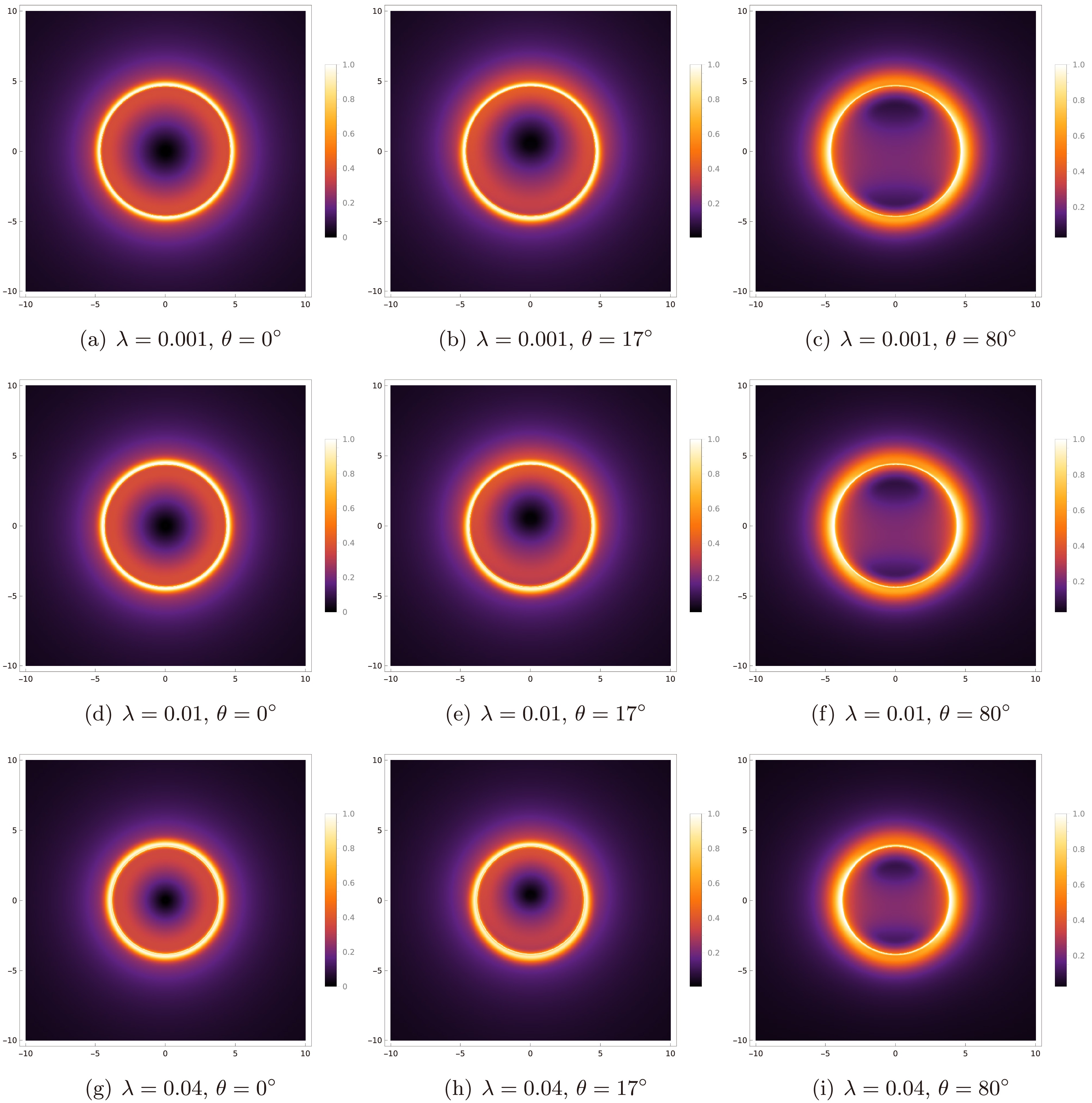
Figure 2. (color online) Black hole shadow images for the phenomenological model under isotropic radiation. The accretion flow is in the infalling-motion mode, with an observation frequency of 230 GHz and
$ M = 1 $ .The dependence of the black hole shadow image on the non-commutative parameter λ and the inclination angle θ is shown in Fig. 2. Morphologically, the inclination angle θ plays a decisive role in shaping the image brightness distribution. When the viewing angle is nearly face-on (
$ \theta \approx 0^{\circ} $ ), the line of sight is nearly orthogonal to the velocity field of the accretion flow. Consequently, the image exhibits a high degree of axisymmetry, with the photon rings appearing as concentric circles with nearly uniform azimuthal brightness. As the inclination increases to a moderate angle ($ \theta = 17^{\circ} $ ), the projected geometry of the accretion flow changes. Although the photon ring remains centered, projection effects from the background accretion flow introduce a weak asymmetry into the overall image. When the inclination is further increased to a nearly edge-on view ($ \theta = 80^{\circ} $ ), the image displays pronounced bilateral symmetry, with the emission being significantly brighter along the horizontal (equatorial) direction than along the vertical direction. This left-right symmetry is a direct consequence of the spherical symmetry of the Schwarzschild spacetime combined with the adopted purely radial infalling motion of the accretion flow.In addition to the inclination effects, the non-commutative parameter λ systematically modifies the geometric scale of the image. A comparison of the panels for different values of λ (
$ 0.001, 0.01, 0.04 $ ) shows that, as λ increases, the overall diameter of the bright higher-order photon rings decreases monotonically, and the position of the brightness peak shifts inward. This visual contraction is in excellent agreement with the theoretical analysis of the geometric quantities presented earlier, directly reflecting the physical reduction of the photon sphere radius$ r_{\mathrm{ph}} $ and the critical impact parameter$ b_c $ induced by spacetime non-commutativity.To quantitatively validate the large-scale image features presented in Fig. 2, we extract the corresponding one-dimensional intensity profiles, as shown in Fig. 3. Across all subfigures, the intensity curves exhibit a pronounced bimodal structure, with two sharp peaks that delineate the bright cross sections of the photon ring. Comparing the profiles for different non-commutative parameters (blue:
$ \lambda = 0.001 $ , red:$ \lambda = 0.01 $ , green:$ \lambda = 0.04 $ ) shows that, as λ increases, the two peaks systematically shift inward, substantially reducing their separation. This behavior is quantitatively consistent with the visual observations in Fig. 2, where the angular diameter of the photon ring decreases monotonically with increasing λ.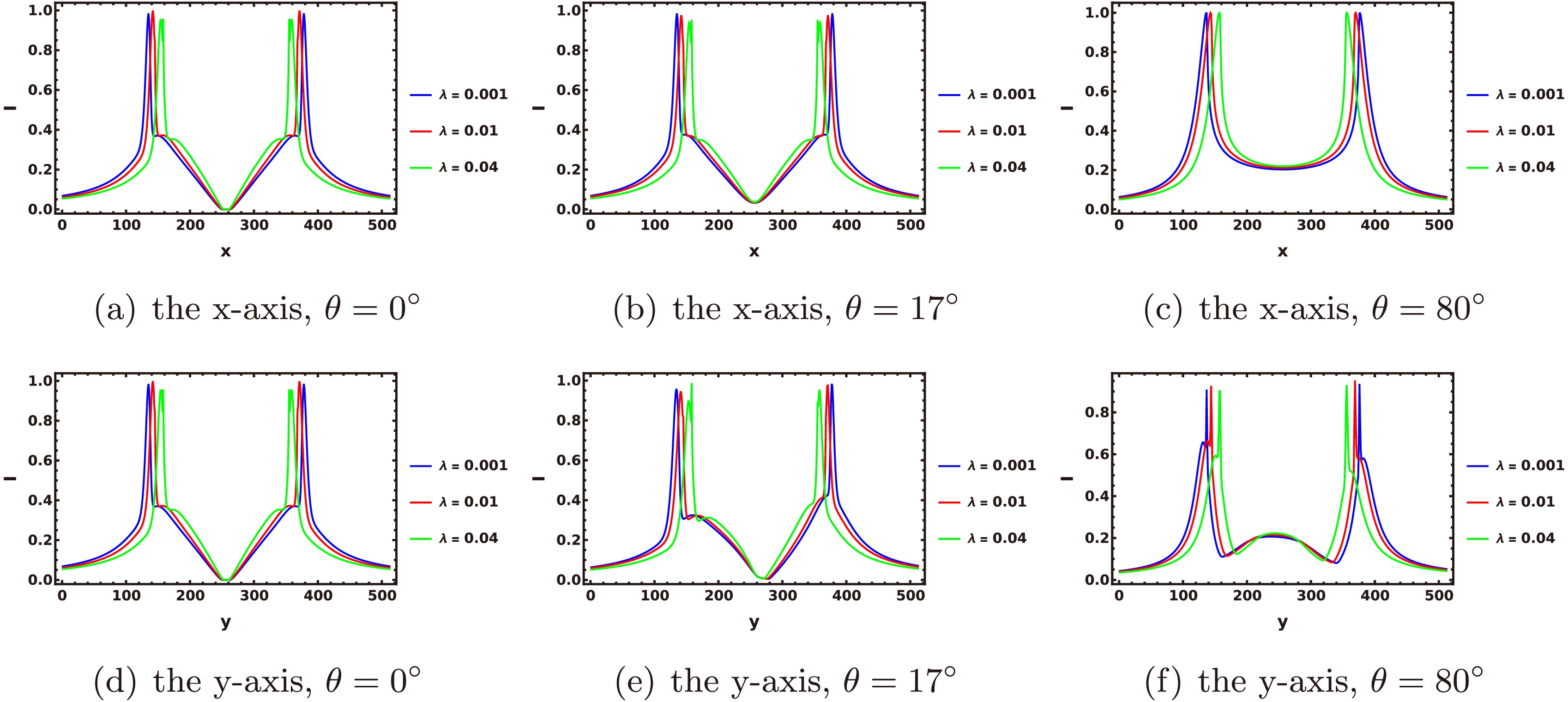
Figure 3. (color online) Intensity distributions along the x- and y-axes for the phenomenological model under isotropic radiation. The accretion flow is in the infall mode.
Furthermore, the modulation of the profile shape by the inclination angle θ reveals the distinctive geometric characteristics of the accretion-flow emission. In the horizontal profile at a nearly edge-on inclination (
$ \theta = 80^{\circ} $ , Fig. 3(c)), the left and right peak heights remain highly symmetric, and the peaks are significantly brighter than those in the vertical profile (Fig. 3(f)). Notably, in this high-inclination vertical profile (Fig. 3(f)), a distinct local maximum emerges in the central region of the shadow between the two main peaks, giving the curve a characteristic ''W" shape. This feature corresponds to the diffuse background light observed at the center of the shadow in Fig. 2. It confirms that, in the geometrically thick accretion disk model, the line of sight passes through gravitationally lensed, overlapping emission regions located above and below the equatorial plane. Thus, the profile analysis in Fig. 3 not only quantitatively corroborates the two-dimensional imaging results but also clearly reflects the complex coupling between the three-dimensional geometry of the accretion flow and strong gravitational lensing effects.To simulate the finite resolution of realistic observational instruments, we apply Gaussian convolution to the high-resolution images shown in Fig. 2. This convolution substantially modifies the morphological characteristics of the images. Owing to the simulated diffraction limit, the extremely sharp and bright higher-order photon ring structures visible in the original images are completely smoothed, merging with the surrounding diffuse primary emission to form a broad, continuous ring-like feature. The initially sharp boundary of the event horizon shadow is also blurred, transitioning into a central dark region characterized by a smooth intensity gradient. However, although the fine structures at sub-microarcsecond scales are washed out, the macroscopic geometric imprint induced by spacetime non-commutativity remains robustly preserved. A comparison of the three panels in Fig. 4 clearly shows that, as the non-commutative parameter λ increases, both the overall contour of the blurred ring and the central shadow region it encloses continue to exhibit systematic contraction. To systematically track the observational signatures as the spacetime approaches the extremal state under the isotropic radiation model, we extend our numerical simulations to parameter values near the critical boundary, specifically
$\lambda \in \{0.047,\; 0.048, 0.049\} M^2 $ . This selection ensures that the central object remains within the valid regime of a regular black hole ($\lambda \le \lambda_c $ ). Figure 5 illustrates the resulting shadow images and specific intensity profiles. In the two-dimensional shadow images, a distinct inward-shrinking trend is evident in both the bright photon ring and the central shadow region as$\lambda $ increases toward the critical value$\lambda_c \approx 0.049 $ . This geometric deformation is quantitatively confirmed by the one-dimensional specific intensity curves, in which the separation between the two sharp photon-ring peaks gradually decreases and the peak positions shift toward the image center. In addition to this geometric contraction, the peak specific intensity of the photon ring increases with$\lambda $ , with the curve for$\lambda = 0.049 $ attaining the highest value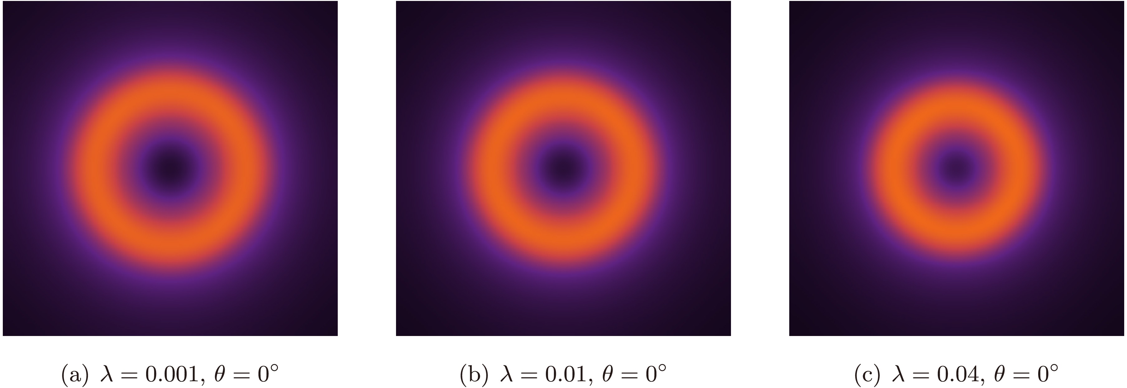
Figure 4. (color online) Black-hole images blurred with a Gaussian filter whose standard deviation is set to
$ 1/12 $ of the field of view,$ \alpha_{\mathrm{fov}} $ . The plotting parameters are consistent with those in Fig. 2. -
We first discuss the imaging characteristics of the accretion flow around a non-commutative Schwarzschild black hole under the assumption of isotropic emission. The simulation assumes that the accretion flow undergoes radial infall, and the observation frequency is fixed at 230 GHz. Figure 2 shows the black hole shadow images for different inclination angles θ (
$ 0^\circ, 17^\circ, 80^\circ $ ) and various values of the non-commutative parameter λ. All images exhibit pronounced layered structures, including bright higher-order images formed by strongly lensed photons and a diffuse primary image formed by directly propagating photons. Within the higher-order images, there is a region with a significant intensity decrease. For a geometrically thin disk, this region typically corresponds to a sharply defined inner shadow [64]. However, because we adopt a geometrically thick accretion disk model in this study, the emitting material outside the equatorial plane partially fills the line of sight. Consequently, this region is not completely dark; rather, it appears as a relatively shaded central area.
Figure 2. (color online) Black hole shadow images for the phenomenological model under isotropic radiation. The accretion flow is in the infalling-motion mode, with an observation frequency of 230 GHz and
$ M = 1 $ .The dependence of the black hole shadow image on the non-commutative parameter λ and the inclination angle θ is shown in Fig. 2. Morphologically, the inclination angle θ plays a decisive role in shaping the image brightness distribution. When the viewing angle is nearly face-on (
$ \theta \approx 0^{\circ} $ ), the line of sight is nearly orthogonal to the velocity field of the accretion flow. Consequently, the image exhibits a high degree of axisymmetry, with the photon rings appearing as concentric circles with nearly uniform azimuthal brightness. As the inclination increases to a moderate angle ($ \theta = 17^{\circ} $ ), the projected geometry of the accretion flow changes. Although the photon ring remains centered, projection effects from the background accretion flow introduce a weak asymmetry into the overall image. When the inclination is further increased to a nearly edge-on view ($ \theta = 80^{\circ} $ ), the image displays pronounced bilateral symmetry, with the emission being significantly brighter along the horizontal (equatorial) direction than along the vertical direction. This left-right symmetry is a direct consequence of the spherical symmetry of the Schwarzschild spacetime combined with the adopted purely radial infalling motion of the accretion flow.In addition to the inclination effects, the non-commutative parameter λ systematically modifies the geometric scale of the image. A comparison of the panels for different values of λ (
$ 0.001, 0.01, 0.04 $ ) shows that, as λ increases, the overall diameter of the bright higher-order photon rings decreases monotonically, and the position of the brightness peak shifts inward. This visual contraction is in excellent agreement with the theoretical analysis of the geometric quantities presented earlier, directly reflecting the physical reduction of the photon sphere radius$ r_{\mathrm{ph}} $ and the critical impact parameter$ b_c $ induced by spacetime non-commutativity.To quantitatively validate the large-scale image features presented in Fig. 2, we extract the corresponding one-dimensional intensity profiles, as shown in Fig. 3. Across all subfigures, the intensity curves exhibit a pronounced bimodal structure, with two sharp peaks that delineate the bright cross sections of the photon ring. Comparing the profiles for different non-commutative parameters (blue:
$ \lambda = 0.001 $ , red:$ \lambda = 0.01 $ , green:$ \lambda = 0.04 $ ) shows that, as λ increases, the two peaks systematically shift inward, substantially reducing their separation. This behavior is quantitatively consistent with the visual observations in Fig. 2, where the angular diameter of the photon ring decreases monotonically with increasing λ.
Figure 3. (color online) Intensity distributions along the x- and y-axes for the phenomenological model under isotropic radiation. The accretion flow is in the infall mode.
Furthermore, the modulation of the profile shape by the inclination angle θ reveals the distinctive geometric characteristics of the accretion-flow emission. In the horizontal profile at a nearly edge-on inclination (
$ \theta = 80^{\circ} $ , Fig. 3(c)), the left and right peak heights remain highly symmetric, and the peaks are significantly brighter than those in the vertical profile (Fig. 3(f)). Notably, in this high-inclination vertical profile (Fig. 3(f)), a distinct local maximum emerges in the central region of the shadow between the two main peaks, giving the curve a characteristic ''W" shape. This feature corresponds to the diffuse background light observed at the center of the shadow in Fig. 2. It confirms that, in the geometrically thick accretion disk model, the line of sight passes through gravitationally lensed, overlapping emission regions located above and below the equatorial plane. Thus, the profile analysis in Fig. 3 not only quantitatively corroborates the two-dimensional imaging results but also clearly reflects the complex coupling between the three-dimensional geometry of the accretion flow and strong gravitational lensing effects.To simulate the finite resolution of realistic observational instruments, we apply Gaussian convolution to the high-resolution images shown in Fig. 2. This convolution substantially modifies the morphological characteristics of the images. Owing to the simulated diffraction limit, the extremely sharp and bright higher-order photon ring structures visible in the original images are completely smoothed, merging with the surrounding diffuse primary emission to form a broad, continuous ring-like feature. The initially sharp boundary of the event horizon shadow is also blurred, transitioning into a central dark region characterized by a smooth intensity gradient. However, although the fine structures at sub-microarcsecond scales are washed out, the macroscopic geometric imprint induced by spacetime non-commutativity remains robustly preserved. A comparison of the three panels in Fig. 4 clearly shows that, as the non-commutative parameter λ increases, both the overall contour of the blurred ring and the central shadow region it encloses continue to exhibit systematic contraction. To systematically track the observational signatures as the spacetime approaches the extremal state under the isotropic radiation model, we extend our numerical simulations to parameter values near the critical boundary, specifically
$\lambda \in \{0.047,\; 0.048, 0.049\} M^2 $ . This selection ensures that the central object remains within the valid regime of a regular black hole ($\lambda \le \lambda_c $ ). Figure 5 illustrates the resulting shadow images and specific intensity profiles. In the two-dimensional shadow images, a distinct inward-shrinking trend is evident in both the bright photon ring and the central shadow region as$\lambda $ increases toward the critical value$\lambda_c \approx 0.049 $ . This geometric deformation is quantitatively confirmed by the one-dimensional specific intensity curves, in which the separation between the two sharp photon-ring peaks gradually decreases and the peak positions shift toward the image center. In addition to this geometric contraction, the peak specific intensity of the photon ring increases with$\lambda $ , with the curve for$\lambda = 0.049 $ attaining the highest value
Figure 4. (color online) Black-hole images blurred with a Gaussian filter whose standard deviation is set to
$ 1/12 $ of the field of view,$ \alpha_{\mathrm{fov}} $ . The plotting parameters are consistent with those in Fig. 2. -
We first discuss the imaging characteristics of the accretion flow around a non-commutative Schwarzschild black hole under the assumption of isotropic emission. The simulation assumes that the accretion flow undergoes radial infall, and the observation frequency is fixed at 230 GHz. Figure 2 shows the black hole shadow images for different inclination angles θ (
$ 0^\circ, 17^\circ, 80^\circ $ ) and various values of the non-commutative parameter λ. All images exhibit pronounced layered structures, including bright higher-order images formed by strongly lensed photons and a diffuse primary image formed by directly propagating photons. Within the higher-order images, there is a region with a significant intensity decrease. For a geometrically thin disk, this region typically corresponds to a sharply defined inner shadow [64]. However, because we adopt a geometrically thick accretion disk model in this study, the emitting material outside the equatorial plane partially fills the line of sight. Consequently, this region is not completely dark; rather, it appears as a relatively shaded central area.
Figure 2. (color online) Black hole shadow images for the phenomenological model under isotropic radiation. The accretion flow is in the infalling-motion mode, with an observation frequency of 230 GHz and
$ M = 1 $ .The dependence of the black hole shadow image on the non-commutative parameter λ and the inclination angle θ is shown in Fig. 2. Morphologically, the inclination angle θ plays a decisive role in shaping the image brightness distribution. When the viewing angle is nearly face-on (
$ \theta \approx 0^{\circ} $ ), the line of sight is nearly orthogonal to the velocity field of the accretion flow. Consequently, the image exhibits a high degree of axisymmetry, with the photon rings appearing as concentric circles with nearly uniform azimuthal brightness. As the inclination increases to a moderate angle ($ \theta = 17^{\circ} $ ), the projected geometry of the accretion flow changes. Although the photon ring remains centered, projection effects from the background accretion flow introduce a weak asymmetry into the overall image. When the inclination is further increased to a nearly edge-on view ($ \theta = 80^{\circ} $ ), the image displays pronounced bilateral symmetry, with the emission being significantly brighter along the horizontal (equatorial) direction than along the vertical direction. This left-right symmetry is a direct consequence of the spherical symmetry of the Schwarzschild spacetime combined with the adopted purely radial infalling motion of the accretion flow.In addition to the inclination effects, the non-commutative parameter λ systematically modifies the geometric scale of the image. A comparison of the panels for different values of λ (
$ 0.001, 0.01, 0.04 $ ) shows that, as λ increases, the overall diameter of the bright higher-order photon rings decreases monotonically, and the position of the brightness peak shifts inward. This visual contraction is in excellent agreement with the theoretical analysis of the geometric quantities presented earlier, directly reflecting the physical reduction of the photon sphere radius$ r_{\mathrm{ph}} $ and the critical impact parameter$ b_c $ induced by spacetime non-commutativity.To quantitatively validate the large-scale image features presented in Fig. 2, we extract the corresponding one-dimensional intensity profiles, as shown in Fig. 3. Across all subfigures, the intensity curves exhibit a pronounced bimodal structure, with two sharp peaks that delineate the bright cross sections of the photon ring. Comparing the profiles for different non-commutative parameters (blue:
$ \lambda = 0.001 $ , red:$ \lambda = 0.01 $ , green:$ \lambda = 0.04 $ ) shows that, as λ increases, the two peaks systematically shift inward, substantially reducing their separation. This behavior is quantitatively consistent with the visual observations in Fig. 2, where the angular diameter of the photon ring decreases monotonically with increasing λ.
Figure 3. (color online) Intensity distributions along the x- and y-axes for the phenomenological model under isotropic radiation. The accretion flow is in the infall mode.
Furthermore, the modulation of the profile shape by the inclination angle θ reveals the distinctive geometric characteristics of the accretion-flow emission. In the horizontal profile at a nearly edge-on inclination (
$ \theta = 80^{\circ} $ , Fig. 3(c)), the left and right peak heights remain highly symmetric, and the peaks are significantly brighter than those in the vertical profile (Fig. 3(f)). Notably, in this high-inclination vertical profile (Fig. 3(f)), a distinct local maximum emerges in the central region of the shadow between the two main peaks, giving the curve a characteristic ''W" shape. This feature corresponds to the diffuse background light observed at the center of the shadow in Fig. 2. It confirms that, in the geometrically thick accretion disk model, the line of sight passes through gravitationally lensed, overlapping emission regions located above and below the equatorial plane. Thus, the profile analysis in Fig. 3 not only quantitatively corroborates the two-dimensional imaging results but also clearly reflects the complex coupling between the three-dimensional geometry of the accretion flow and strong gravitational lensing effects.To simulate the finite resolution of realistic observational instruments, we apply Gaussian convolution to the high-resolution images shown in Fig. 2. This convolution substantially modifies the morphological characteristics of the images. Owing to the simulated diffraction limit, the extremely sharp and bright higher-order photon ring structures visible in the original images are completely smoothed, merging with the surrounding diffuse primary emission to form a broad, continuous ring-like feature. The initially sharp boundary of the event horizon shadow is also blurred, transitioning into a central dark region characterized by a smooth intensity gradient. However, although the fine structures at sub-microarcsecond scales are washed out, the macroscopic geometric imprint induced by spacetime non-commutativity remains robustly preserved. A comparison of the three panels in Fig. 4 clearly shows that, as the non-commutative parameter λ increases, both the overall contour of the blurred ring and the central shadow region it encloses continue to exhibit systematic contraction. To systematically track the observational signatures as the spacetime approaches the extremal state under the isotropic radiation model, we extend our numerical simulations to parameter values near the critical boundary, specifically
$\lambda \in \{0.047,\; 0.048, 0.049\} M^2 $ . This selection ensures that the central object remains within the valid regime of a regular black hole ($\lambda \le \lambda_c $ ). Figure 5 illustrates the resulting shadow images and specific intensity profiles. In the two-dimensional shadow images, a distinct inward-shrinking trend is evident in both the bright photon ring and the central shadow region as$\lambda $ increases toward the critical value$\lambda_c \approx 0.049 $ . This geometric deformation is quantitatively confirmed by the one-dimensional specific intensity curves, in which the separation between the two sharp photon-ring peaks gradually decreases and the peak positions shift toward the image center. In addition to this geometric contraction, the peak specific intensity of the photon ring increases with$\lambda $ , with the curve for$\lambda = 0.049 $ attaining the highest value
Figure 4. (color online) Black-hole images blurred with a Gaussian filter whose standard deviation is set to
$ 1/12 $ of the field of view,$ \alpha_{\mathrm{fov}} $ . The plotting parameters are consistent with those in Fig. 2. -
To comprehensively evaluate the influence of different radiation mechanisms on the imaging results, Fig. 6 presents the simulated images under anisotropic radiation conditions. Similar to the isotropic case, each panel in Fig. 6 shows a distinct bright ring, corresponding precisely to the sharp peaks in the intensity profiles in Fig. 7. At a given inclination θ, an increase in the non-commutative parameter λ consistently leads to a systematic decrease in the diameter of the bright ring. This trend is quantitatively confirmed in Fig. 7, where the peak shifts for the different curves follow exactly the same pattern as that observed in Fig. 3. This robustly demonstrates that the ring shrinkage is an intrinsic geometric effect primarily governed by the underlying spacetime metric. Conversely, for a fixed λ, varying θ reveals a key difference between the two radiation models. At small inclinations (
$ \theta \approx 0^{\circ} $ and$ 17^{\circ} $ ), the anisotropic model exhibits a morphological evolution nearly identical to that of the isotropic model, with the image features remaining highly consistent. However, at the nearly edge-on inclination of$ \theta = 80^{\circ} $ , a significant divergence emerges. In the isotropic model, the higher-order images, although asymmetric, remain approximately ring-shaped. In contrast, under the anisotropic model, owing to the strong dependence of the radiation intensity on the emission angle, the higher-order images are visibly deformed into an ellipsoidal shape. Furthermore, emission from regions outside the equatorial plane more strongly obscures the central dark region, resulting in a more uniform internal brightness distribution. This effect is quantitatively supported by the elevated central extrema in the vertical profiles in Fig. 7. These findings indicate that, as the viewing angle approaches the plane of the accretion disk, the directionality of the radiation field exerts a non-negligible modulating effect on the shadow morphology.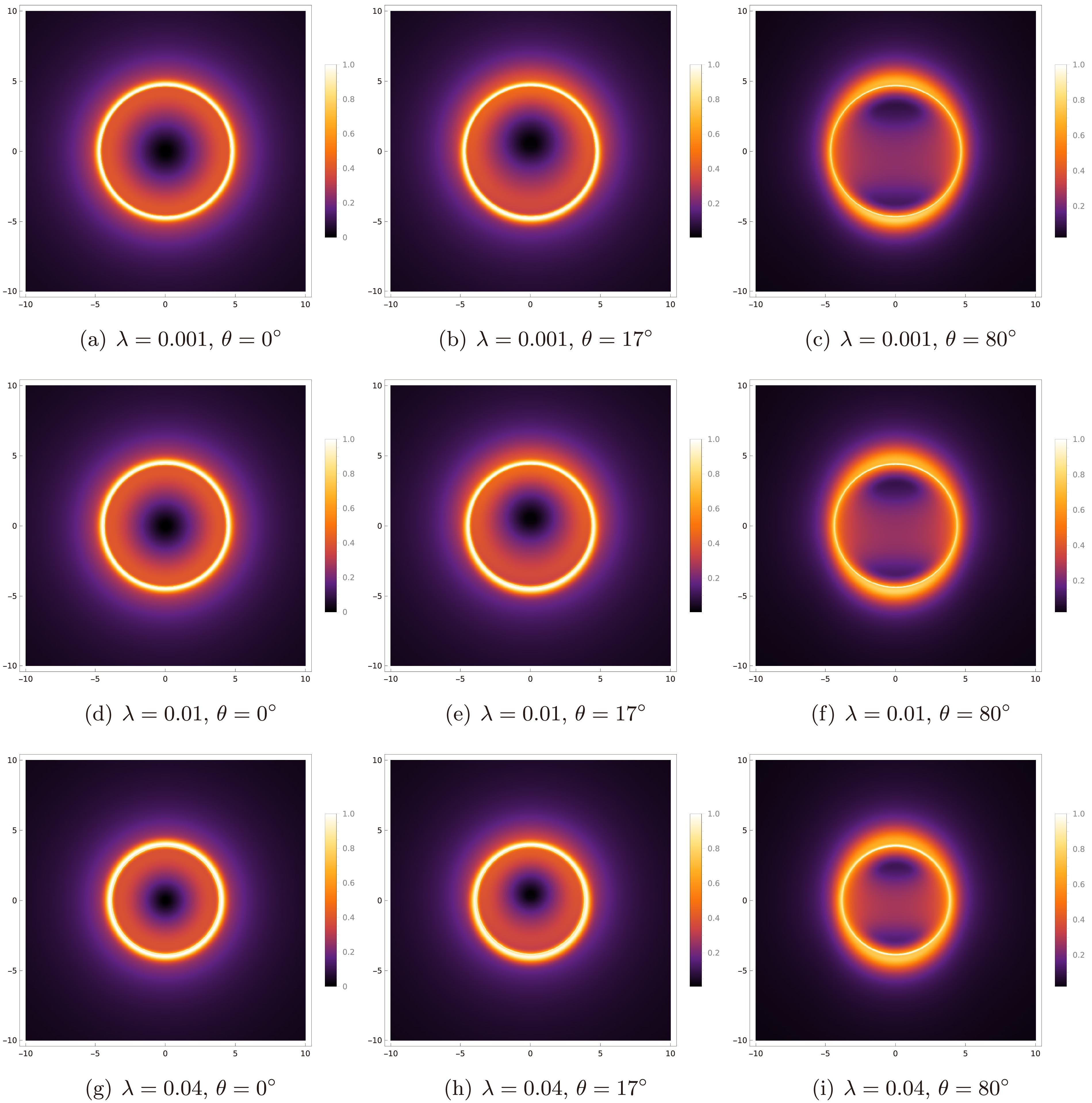
Figure 6. (color online) Black hole shadow images of the phenomenological model under anisotropic radiation. The accretion flow is in the infalling-motion mode, with an observing frequency of 230 GHz and
$ M = 1 $ .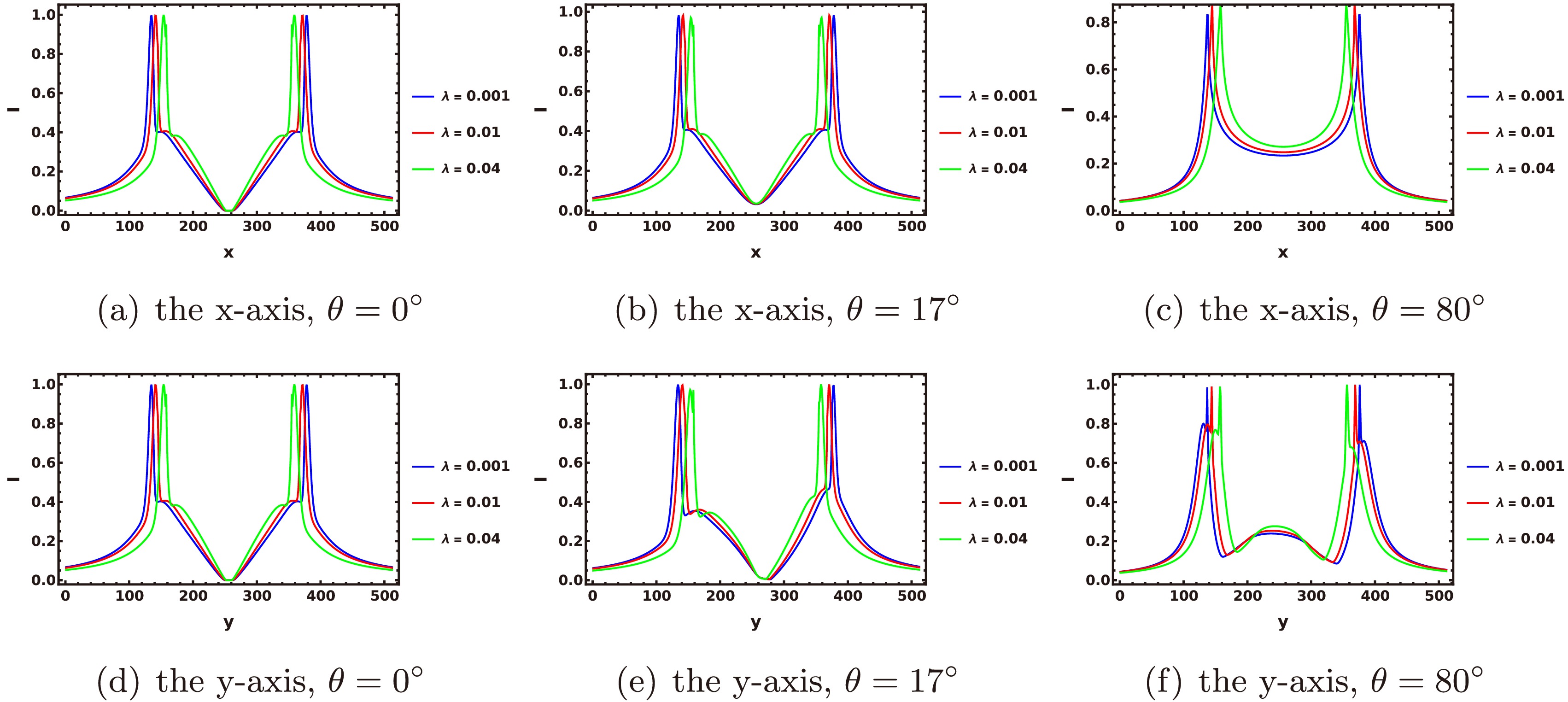
Figure 7. (color online) Intensity distributions along the x- and y-axes for the phenomenological model under anisotropic radiation. The accretion flow is in the infalling-motion mode.
Furthermore, we examine the near-extremal scenario for the anisotropic radiation model with
$\lambda \in \{0.047, 0.048,\; 0.049\} M^2 $ , as displayed in Fig. 8. Similar to the isotropic case shown in Fig. 5, the bright photon ring and central shadow region exhibit noticeable contraction accompanied by intensity enhancement as$\lambda \to \lambda_c $ . Crucially, the strong agreement between the isotropic and anisotropic scenarios demonstrates that both the structural contraction and the intensity enhancement are strictly governed by the underlying spacetime geometry and are unaffected by the specific emission mechanisms of the accretion flow. Ultimately, this evolutionary trend continues until the extremal state is reached, where the photon sphere radius$r_{\mathrm{ph}} $ and the critical impact parameter$b_c $ contract to their absolute minima, thereby establishing a strict theoretical lower bound for the apparent shadow size of the non-commutative black hole.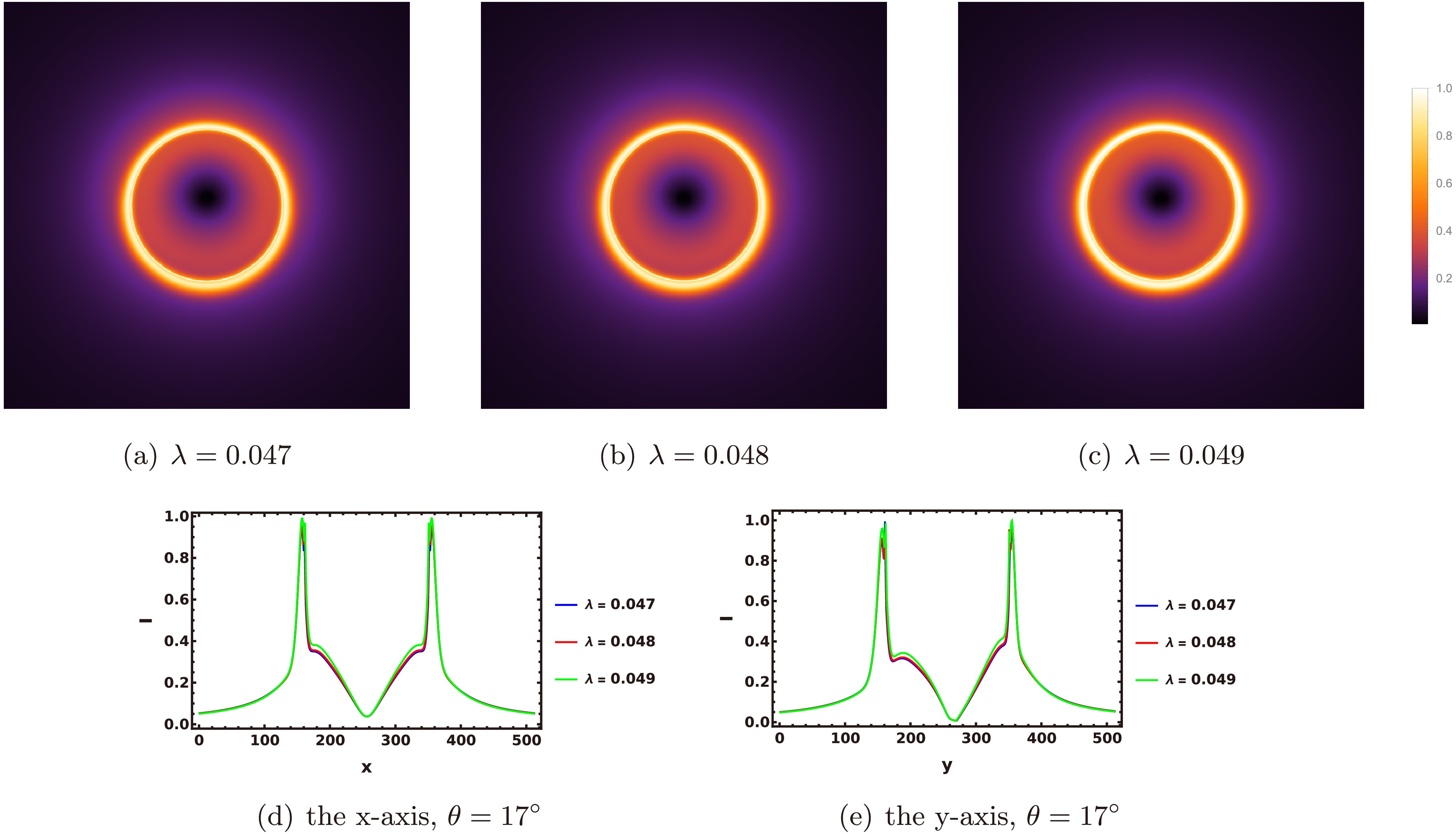
Figure 5. (color online) Black hole shadow images of the phenomenological model under isotropic radiation. Panels (a), (b), and (c) show the two-dimensional shadow images. The accretion flow is in the infalling-motion mode, with an observing frequency of
$ 230 $ GHz,$ M=1 $ , and an inclination angle of$ \theta = 17^\circ $ . Panels (d) and (e) show the one-dimensional specific-intensity profiles along the horizontal (x-axis) and vertical (y-axis) directions of the image plane, respectively, at an inclination angle of$ \theta = 17^\circ $ .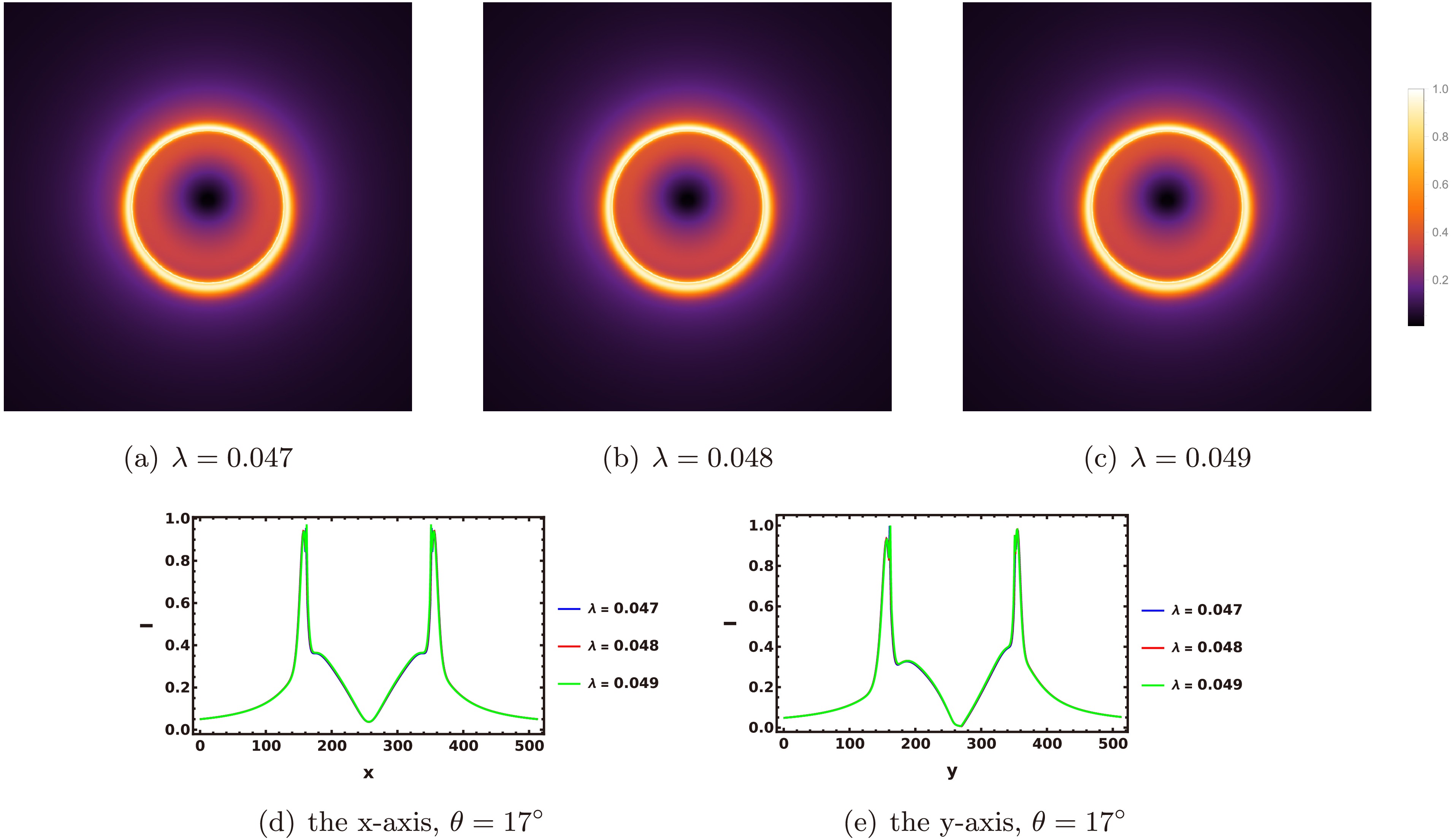
Figure 8. (color online) Black hole shadow images of the phenomenological model under anisotropic radiation. Panels (a), (b), and (c) show the two-dimensional shadow images. The accretion flow is in the infalling motion mode, with an observation frequency of
$ 230 $ GHz,$ M=1 $ , and an inclination angle of$ \theta = 17^\circ $ . Panels (d) and (e) show the one-dimensional specific intensity profiles along the horizontal (x-axis) and vertical (y-axis) directions of the image plane, respectively, for an inclination angle of$ \theta = 17^\circ $ . -
To comprehensively evaluate the influence of different radiation mechanisms on the imaging results, Fig. 6 presents the simulated images under anisotropic radiation conditions. Similar to the isotropic case, each panel in Fig. 6 shows a distinct bright ring, corresponding precisely to the sharp peaks in the intensity profiles in Fig. 7. At a given inclination θ, an increase in the non-commutative parameter λ consistently leads to a systematic decrease in the diameter of the bright ring. This trend is quantitatively confirmed in Fig. 7, where the peak shifts for the different curves follow exactly the same pattern as that observed in Fig. 3. This robustly demonstrates that the ring shrinkage is an intrinsic geometric effect primarily governed by the underlying spacetime metric. Conversely, for a fixed λ, varying θ reveals a key difference between the two radiation models. At small inclinations (
$ \theta \approx 0^{\circ} $ and$ 17^{\circ} $ ), the anisotropic model exhibits a morphological evolution nearly identical to that of the isotropic model, with the image features remaining highly consistent. However, at the nearly edge-on inclination of$ \theta = 80^{\circ} $ , a significant divergence emerges. In the isotropic model, the higher-order images, although asymmetric, remain approximately ring-shaped. In contrast, under the anisotropic model, owing to the strong dependence of the radiation intensity on the emission angle, the higher-order images are visibly deformed into an ellipsoidal shape. Furthermore, emission from regions outside the equatorial plane more strongly obscures the central dark region, resulting in a more uniform internal brightness distribution. This effect is quantitatively supported by the elevated central extrema in the vertical profiles in Fig. 7. These findings indicate that, as the viewing angle approaches the plane of the accretion disk, the directionality of the radiation field exerts a non-negligible modulating effect on the shadow morphology.
Figure 6. (color online) Black hole shadow images of the phenomenological model under anisotropic radiation. The accretion flow is in the infalling-motion mode, with an observing frequency of 230 GHz and
$ M = 1 $ .
Figure 7. (color online) Intensity distributions along the x- and y-axes for the phenomenological model under anisotropic radiation. The accretion flow is in the infalling-motion mode.
Furthermore, we examine the near-extremal scenario for the anisotropic radiation model with
$\lambda \in \{0.047, 0.048,\; 0.049\} M^2 $ , as displayed in Fig. 8. Similar to the isotropic case shown in Fig. 5, the bright photon ring and central shadow region exhibit noticeable contraction accompanied by intensity enhancement as$\lambda \to \lambda_c $ . Crucially, the strong agreement between the isotropic and anisotropic scenarios demonstrates that both the structural contraction and the intensity enhancement are strictly governed by the underlying spacetime geometry and are unaffected by the specific emission mechanisms of the accretion flow. Ultimately, this evolutionary trend continues until the extremal state is reached, where the photon sphere radius$r_{\mathrm{ph}} $ and the critical impact parameter$b_c $ contract to their absolute minima, thereby establishing a strict theoretical lower bound for the apparent shadow size of the non-commutative black hole.
Figure 5. (color online) Black hole shadow images of the phenomenological model under isotropic radiation. Panels (a), (b), and (c) show the two-dimensional shadow images. The accretion flow is in the infalling-motion mode, with an observing frequency of
$ 230 $ GHz,$ M=1 $ , and an inclination angle of$ \theta = 17^\circ $ . Panels (d) and (e) show the one-dimensional specific-intensity profiles along the horizontal (x-axis) and vertical (y-axis) directions of the image plane, respectively, at an inclination angle of$ \theta = 17^\circ $ .
Figure 8. (color online) Black hole shadow images of the phenomenological model under anisotropic radiation. Panels (a), (b), and (c) show the two-dimensional shadow images. The accretion flow is in the infalling motion mode, with an observation frequency of
$ 230 $ GHz,$ M=1 $ , and an inclination angle of$ \theta = 17^\circ $ . Panels (d) and (e) show the one-dimensional specific intensity profiles along the horizontal (x-axis) and vertical (y-axis) directions of the image plane, respectively, for an inclination angle of$ \theta = 17^\circ $ . -
To comprehensively evaluate the influence of different radiation mechanisms on the imaging results, Fig. 6 presents the simulated images under anisotropic radiation conditions. Similar to the isotropic case, each panel in Fig. 6 shows a distinct bright ring, corresponding precisely to the sharp peaks in the intensity profiles in Fig. 7. At a given inclination θ, an increase in the non-commutative parameter λ consistently leads to a systematic decrease in the diameter of the bright ring. This trend is quantitatively confirmed in Fig. 7, where the peak shifts for the different curves follow exactly the same pattern as that observed in Fig. 3. This robustly demonstrates that the ring shrinkage is an intrinsic geometric effect primarily governed by the underlying spacetime metric. Conversely, for a fixed λ, varying θ reveals a key difference between the two radiation models. At small inclinations (
$ \theta \approx 0^{\circ} $ and$ 17^{\circ} $ ), the anisotropic model exhibits a morphological evolution nearly identical to that of the isotropic model, with the image features remaining highly consistent. However, at the nearly edge-on inclination of$ \theta = 80^{\circ} $ , a significant divergence emerges. In the isotropic model, the higher-order images, although asymmetric, remain approximately ring-shaped. In contrast, under the anisotropic model, owing to the strong dependence of the radiation intensity on the emission angle, the higher-order images are visibly deformed into an ellipsoidal shape. Furthermore, emission from regions outside the equatorial plane more strongly obscures the central dark region, resulting in a more uniform internal brightness distribution. This effect is quantitatively supported by the elevated central extrema in the vertical profiles in Fig. 7. These findings indicate that, as the viewing angle approaches the plane of the accretion disk, the directionality of the radiation field exerts a non-negligible modulating effect on the shadow morphology.
Figure 6. (color online) Black hole shadow images of the phenomenological model under anisotropic radiation. The accretion flow is in the infalling-motion mode, with an observing frequency of 230 GHz and
$ M = 1 $ .
Figure 7. (color online) Intensity distributions along the x- and y-axes for the phenomenological model under anisotropic radiation. The accretion flow is in the infalling-motion mode.
Furthermore, we examine the near-extremal scenario for the anisotropic radiation model with
$\lambda \in \{0.047, 0.048,\; 0.049\} M^2 $ , as displayed in Fig. 8. Similar to the isotropic case shown in Fig. 5, the bright photon ring and central shadow region exhibit noticeable contraction accompanied by intensity enhancement as$\lambda \to \lambda_c $ . Crucially, the strong agreement between the isotropic and anisotropic scenarios demonstrates that both the structural contraction and the intensity enhancement are strictly governed by the underlying spacetime geometry and are unaffected by the specific emission mechanisms of the accretion flow. Ultimately, this evolutionary trend continues until the extremal state is reached, where the photon sphere radius$r_{\mathrm{ph}} $ and the critical impact parameter$b_c $ contract to their absolute minima, thereby establishing a strict theoretical lower bound for the apparent shadow size of the non-commutative black hole.
Figure 5. (color online) Black hole shadow images of the phenomenological model under isotropic radiation. Panels (a), (b), and (c) show the two-dimensional shadow images. The accretion flow is in the infalling-motion mode, with an observing frequency of
$ 230 $ GHz,$ M=1 $ , and an inclination angle of$ \theta = 17^\circ $ . Panels (d) and (e) show the one-dimensional specific-intensity profiles along the horizontal (x-axis) and vertical (y-axis) directions of the image plane, respectively, at an inclination angle of$ \theta = 17^\circ $ .
Figure 8. (color online) Black hole shadow images of the phenomenological model under anisotropic radiation. Panels (a), (b), and (c) show the two-dimensional shadow images. The accretion flow is in the infalling motion mode, with an observation frequency of
$ 230 $ GHz,$ M=1 $ , and an inclination angle of$ \theta = 17^\circ $ . Panels (d) and (e) show the one-dimensional specific intensity profiles along the horizontal (x-axis) and vertical (y-axis) directions of the image plane, respectively, for an inclination angle of$ \theta = 17^\circ $ . -
In this work, we investigate the imaging properties of a noncommutative Schwarzschild black hole surrounded by a steady-state, geometrically thick accretion flow. We first systematically review the fundamental properties of this modified spacetime, illustrating how the deformation parameter λ alters the event horizon structure and photon geodesics. We then adopt a geometrically thick, radiatively inefficient accretion flow (RIAF) model to describe a magnetized equilibrium plasma torus. By performing general relativistic ray-tracing and radiative transfer (GRRT) calculations, we obtain the corresponding synthetic black hole images and extract their detailed specific intensity profiles.
The analysis of the isotropic radiation case reveals that the effective spacetime deformation leaves a distinct geometric imprint on the black hole shadow. As the parameter λ increases, the angular diameter of the higher-order images (photon rings) systematically contracts, which appears in the intensity profiles as a significant decrease in the separation between the two sharp peaks. This finding establishes a quantitative link between the macroscopic spacetime parameter and observable imaging features. Moreover, the inclination angle θ significantly modulates the image morphology, which transitions from a highly axisymmetric, perfectly circular ring at
$ \theta \approx 0^{\circ} $ to a structure dominated by geometric projection effects at$ \theta = 80^{\circ} $ . Notably, owing to the adopted radially infalling motion, the images at high inclinations retain bilateral brightness symmetry. The enhanced emission along the equatorial direction primarily arises from the maximized integrated optical path length along the line of sight through the optically thin accretion flow.When incorporating the anisotropic radiation mechanism, we find that the global effects of λ and θ on the shadow size remain qualitatively consistent with those in the isotropic case. However, at a nearly edge-on inclination (
$ \theta = 80^{\circ} $ ), a key morphological divergence emerges. The higher-order photon rings in the isotropic model remain approximately circular, whereas those in the anisotropic model exhibit significant ellipsoidal distortion. Furthermore, obscuration of the central dark region by emission originating outside the equatorial plane is substantially more pronounced in the anisotropic model. These differences indicate that, when interpreting or fitting high-inclination observational data, the directional dependence of the emission mechanism must be carefully accounted for because of its non-negligible modulating effect on the fine structure of the image.In summary, this study demonstrates that effective spacetime regularizations lead to a systematic contraction of the black hole shadow and photon rings, thereby providing an intuitive geometric probe for testing macroscopic spacetime deformations and noncommutative geometric corrections in strong gravitational fields. We caution, however, that shadow size contraction alone may not serve as a unique discriminant, since similar trends are known to emerge in diverse regular black hole models. Breaking this theoretical degeneracy requires exploiting finer observables beyond the apparent shadow diameter. As demonstrated in this work, the detailed morphology of the specific intensity profiles, particularly the peak amplitudes, widths, and radial contrast of the photon ring emission, serves as a crucial diagnostic tool. These intensity distributions directly reflect the higher-order photon ring substructures. Because these features are highly sensitive to the specific form of the metric, they provide effective observational criteria for distinguishing different regular black hole geometries. At the same time, these observational signatures are inevitably entangled with the microphysics of the accretion flow. Resolving this astrophysical degeneracy requires integrating high-resolution three-dimensional GRMHD simulations with multi-wavelength observational data, thereby paving the way toward a clear isolation of macroscopic spacetime deformations from complex plasma backgrounds.
-
In this work, we investigate the imaging properties of a noncommutative Schwarzschild black hole surrounded by a steady-state, geometrically thick accretion flow. We first systematically review the fundamental properties of this modified spacetime, illustrating how the deformation parameter λ alters the event horizon structure and photon geodesics. We then adopt a geometrically thick, radiatively inefficient accretion flow (RIAF) model to describe a magnetized equilibrium plasma torus. By performing general relativistic ray-tracing and radiative transfer (GRRT) calculations, we obtain the corresponding synthetic black hole images and extract their detailed specific intensity profiles.
The analysis of the isotropic radiation case reveals that the effective spacetime deformation leaves a distinct geometric imprint on the black hole shadow. As the parameter λ increases, the angular diameter of the higher-order images (photon rings) systematically contracts, which appears in the intensity profiles as a significant decrease in the separation between the two sharp peaks. This finding establishes a quantitative link between the macroscopic spacetime parameter and observable imaging features. Moreover, the inclination angle θ significantly modulates the image morphology, which transitions from a highly axisymmetric, perfectly circular ring at
$ \theta \approx 0^{\circ} $ to a structure dominated by geometric projection effects at$ \theta = 80^{\circ} $ . Notably, owing to the adopted radially infalling motion, the images at high inclinations retain bilateral brightness symmetry. The enhanced emission along the equatorial direction primarily arises from the maximized integrated optical path length along the line of sight through the optically thin accretion flow.When incorporating the anisotropic radiation mechanism, we find that the global effects of λ and θ on the shadow size remain qualitatively consistent with those in the isotropic case. However, at a nearly edge-on inclination (
$ \theta = 80^{\circ} $ ), a key morphological divergence emerges. The higher-order photon rings in the isotropic model remain approximately circular, whereas those in the anisotropic model exhibit significant ellipsoidal distortion. Furthermore, obscuration of the central dark region by emission originating outside the equatorial plane is substantially more pronounced in the anisotropic model. These differences indicate that, when interpreting or fitting high-inclination observational data, the directional dependence of the emission mechanism must be carefully accounted for because of its non-negligible modulating effect on the fine structure of the image.In summary, this study demonstrates that effective spacetime regularizations lead to a systematic contraction of the black hole shadow and photon rings, thereby providing an intuitive geometric probe for testing macroscopic spacetime deformations and noncommutative geometric corrections in strong gravitational fields. We caution, however, that shadow size contraction alone may not serve as a unique discriminant, since similar trends are known to emerge in diverse regular black hole models. Breaking this theoretical degeneracy requires exploiting finer observables beyond the apparent shadow diameter. As demonstrated in this work, the detailed morphology of the specific intensity profiles, particularly the peak amplitudes, widths, and radial contrast of the photon ring emission, serves as a crucial diagnostic tool. These intensity distributions directly reflect the higher-order photon ring substructures. Because these features are highly sensitive to the specific form of the metric, they provide effective observational criteria for distinguishing different regular black hole geometries. At the same time, these observational signatures are inevitably entangled with the microphysics of the accretion flow. Resolving this astrophysical degeneracy requires integrating high-resolution three-dimensional GRMHD simulations with multi-wavelength observational data, thereby paving the way toward a clear isolation of macroscopic spacetime deformations from complex plasma backgrounds.
-
In this work, we investigate the imaging properties of a noncommutative Schwarzschild black hole surrounded by a steady-state, geometrically thick accretion flow. We first systematically review the fundamental properties of this modified spacetime, illustrating how the deformation parameter λ alters the event horizon structure and photon geodesics. We then adopt a geometrically thick, radiatively inefficient accretion flow (RIAF) model to describe a magnetized equilibrium plasma torus. By performing general relativistic ray-tracing and radiative transfer (GRRT) calculations, we obtain the corresponding synthetic black hole images and extract their detailed specific intensity profiles.
The analysis of the isotropic radiation case reveals that the effective spacetime deformation leaves a distinct geometric imprint on the black hole shadow. As the parameter λ increases, the angular diameter of the higher-order images (photon rings) systematically contracts, which appears in the intensity profiles as a significant decrease in the separation between the two sharp peaks. This finding establishes a quantitative link between the macroscopic spacetime parameter and observable imaging features. Moreover, the inclination angle θ significantly modulates the image morphology, which transitions from a highly axisymmetric, perfectly circular ring at
$ \theta \approx 0^{\circ} $ to a structure dominated by geometric projection effects at$ \theta = 80^{\circ} $ . Notably, owing to the adopted radially infalling motion, the images at high inclinations retain bilateral brightness symmetry. The enhanced emission along the equatorial direction primarily arises from the maximized integrated optical path length along the line of sight through the optically thin accretion flow.When incorporating the anisotropic radiation mechanism, we find that the global effects of λ and θ on the shadow size remain qualitatively consistent with those in the isotropic case. However, at a nearly edge-on inclination (
$ \theta = 80^{\circ} $ ), a key morphological divergence emerges. The higher-order photon rings in the isotropic model remain approximately circular, whereas those in the anisotropic model exhibit significant ellipsoidal distortion. Furthermore, obscuration of the central dark region by emission originating outside the equatorial plane is substantially more pronounced in the anisotropic model. These differences indicate that, when interpreting or fitting high-inclination observational data, the directional dependence of the emission mechanism must be carefully accounted for because of its non-negligible modulating effect on the fine structure of the image.In summary, this study demonstrates that effective spacetime regularizations lead to a systematic contraction of the black hole shadow and photon rings, thereby providing an intuitive geometric probe for testing macroscopic spacetime deformations and noncommutative geometric corrections in strong gravitational fields. We caution, however, that shadow size contraction alone may not serve as a unique discriminant, since similar trends are known to emerge in diverse regular black hole models. Breaking this theoretical degeneracy requires exploiting finer observables beyond the apparent shadow diameter. As demonstrated in this work, the detailed morphology of the specific intensity profiles, particularly the peak amplitudes, widths, and radial contrast of the photon ring emission, serves as a crucial diagnostic tool. These intensity distributions directly reflect the higher-order photon ring substructures. Because these features are highly sensitive to the specific form of the metric, they provide effective observational criteria for distinguishing different regular black hole geometries. At the same time, these observational signatures are inevitably entangled with the microphysics of the accretion flow. Resolving this astrophysical degeneracy requires integrating high-resolution three-dimensional GRMHD simulations with multi-wavelength observational data, thereby paving the way toward a clear isolation of macroscopic spacetime deformations from complex plasma backgrounds.
Optical observational characteristics of a Non-commutative Schwarzschild black hole encircled by thick accretion disks
- Received Date: 2026-05-12
- Available Online: 2026-10-15
Abstract: In this paper, we investigate the imaging properties of non-commutative Schwarzschild black holes surrounded by geometrically thick accretion flows. We employ a phenomenological radiatively inefficient accretion flow model to describe the accreting material. Using general relativistic radiative transfer, we calculate the synchrotron emission from thermal electrons and obtain black hole images at horizon scales. The results indicate that an increase in the non-commutative parameter λ reduces the photon ring size, which substantially decreases the spacing between the two highest peaks in the intensity distribution curve. Moreover, as the observer's inclination angle increases, the image transitions from an axisymmetric ring to a high-inclination structure with pronounced variations in brightness and morphology. Under high-inclination conditions, the anisotropic radiation model yields a notably elliptical deformation of the photon ring, and the contribution of off-equatorial radiation to the central dark region is substantially enhanced compared with that in the isotropic model. These results provide a reference framework for investigating the effects of spacetime non-commutativity in strong gravitational fields.



 DownLoad: