


 Abstract
 HTML
HTML Reference
 Related
 PDF
PDF


-
Quantum chromodynamics (QCD) is believed to be the fundamental theory of the strong interaction. In regimes of interest for heavy-ion collisions and compact-star physics, the coupling is large, and controlled calculations are scarce. Lattice QCD provides high-quality results for the equation of state (EoS) at finite temperature; see, e.g., Ref. [1] for a review. However, at finite baryon chemical potential
$ \mu_B $ , the sign problem limits direct simulations, which motivates effective descriptions that can be confronted with lattice data and extrapolated to finite density. For continuum perspectives at finite temperature and density, see, e.g., Ref. [2].Based on the AdS/CFT correspondence [3], the holographic QCD method provides a useful non-perturbative approach to explore QCD matter under extreme conditions, such as finite temperature and/or baryon density, magnetic, and vortical fields [4−25]. In bottom-up constructions, the Einstein–Maxwell–dilaton (EMD) framework is widely used, where the dilaton field provides an effective description of the gluodynamics, and the model can be calibrated to lattice thermodynamics by choosing the dilaton potential and the gauge kinetic function. To incorporate chiral physics and flavor dynamics in addition to the gluon sector, one usually supplements the EMD background with a flavor action containing a bulk scalar field dual to
$ \bar q q $ , as in the hard-wall/soft-wall models [26, 27], and their improved variants for chiral symmetry breaking and restoration [28].The original soft-wall model introduced by Andreas Karch, Emanuel Katz, Dam T. Son, and Mikhail A. Stephanov [27], often referred to as the Karch–Katz– Son–Stephanov (KKSS) model, provides a simple framework for light-flavor hadron spectra and chiral dynamics, and it also serves as a convenient starting point for improved soft-wall constructions. In many applications, the KKSS sector is treated as a probe: one first solves the EMD background and then evaluates the flavor contribution on top of it. This is efficient and often sufficient for qualitative studies. A more self-consistent description requires the back-reaction of the flavor sector on the geometry. In practice, solving the coupled EMD
$ + $ KKSS system while keeping a single action fixed across thermodynamic states, and simultaneously calibrating to lattice EoS data, is technically nontrivial. As a result, systematic back-reacted studies remain comparatively limited. In particular, it is challenging to calibrate a coupled EMD$ + $ flavor setup to lattice thermodynamics while keeping a single five-dimensional action fixed across thermodynamic states. This motivates a controlled back-reaction study within a fixed EMD$ + $ KKSS action, which is one of the main focuses of this work.In this work, we report three related studies within a single EMD
$ + $ KKSS framework. We first work in the probe approximation and calibrate the EMD model to the lattice EoS of$ (2+1) $ -flavor QCD at finite T and finite$ \mu_B $ by using a neural ordinary differential equation (neural ODE) approach [21, 29−31], and subsequently fit the trained neural networks into explicit analytical expressions. We then treat the EMD system as an effective description of pure Yang–Mills theory and fix its parameters by fitting the$ \mu_B=0 $ lattice pure-glue EoS via a hybrid optimization strategy; see also recent data-driven Einstein–dilaton reconstructions of pure-glue thermodynamics [32]. Finally, we go beyond the probe approximation and solve the coupled EMD$ + $ KKSS equations with back-reaction. With the EMD sector fixed by the pure-glue calibration, we vary the KKSS couplings and compare the resulting$ \mu_B=0 $ EoS with the two-flavor lattice data. A visible mismatch remains, which we view as a structural diagnostic for the present flavor-sector truncation. Moreover, by examining the high-temperature behavior, we find that the back-reacted dimensionless ratios approach a nearly$ \beta_1 $ -insensitive plateau close to the$ \beta_1=0 $ (pure-glue) baseline, which provides a simple diagnostic for the present flavor-sector truncation.This paper is organized as follows. In Sec. II we introduce the EMD
$ + $ KKSS setup and the thermodynamic dictionary. In Sec. III we present the probe-approximation calibration for$ (2+1) $ flavors at finite T and$ \mu_B $ using neural ODE. In Sec. IV we present the pure-glue calibration of the EMD sector at$ \mu_B=0 $ . In Sec. V we describe the coupled EMD$ + $ KKSS system with back-reaction and compare with the two-flavor$ \mu_B=0 $ lattice EoS. We conclude and discuss outlook in Sec. VI. -
Quantum chromodynamics (QCD) is believed to be the fundamental theory of the strong interaction. In regimes of interest for heavy-ion collisions and compact-star physics, the coupling is large, and controlled calculations are scarce. Lattice QCD provides high-quality results for the equation of state (EoS) at finite temperature; see, e.g., Ref. [1] for a review. However, at finite baryon chemical potential
$ \mu_B $ , the sign problem limits direct simulations, which motivates effective descriptions that can be confronted with lattice data and extrapolated to finite density. For continuum perspectives at finite temperature and density, see, e.g., Ref. [2].Based on the AdS/CFT correspondence [3], the holographic QCD method provides a useful non-perturbative approach to explore QCD matter under extreme conditions, such as finite temperature and/or baryon density, magnetic, and vortical fields [4−25]. In bottom-up constructions, the Einstein–Maxwell–dilaton (EMD) framework is widely used, where the dilaton field provides an effective description of the gluodynamics, and the model can be calibrated to lattice thermodynamics by choosing the dilaton potential and the gauge kinetic function. To incorporate chiral physics and flavor dynamics in addition to the gluon sector, one usually supplements the EMD background with a flavor action containing a bulk scalar field dual to
$ \bar q q $ , as in the hard-wall/soft-wall models [26, 27], and their improved variants for chiral symmetry breaking and restoration [28].The original soft-wall model introduced by Andreas Karch, Emanuel Katz, Dam T. Son, and Mikhail A. Stephanov [27], often referred to as the Karch–Katz–Son–Stephanov (KKSS) model, provides a simple framework for light-flavor hadron spectra and chiral dynamics, and it also serves as a convenient starting point for improved soft-wall constructions. In many applications, the KKSS sector is treated as a probe: one first solves the EMD background and then evaluates the flavor contribution on top of it. This is efficient and often sufficient for qualitative studies. A more self-consistent description requires the back-reaction of the flavor sector on the geometry. In practice, solving the coupled EMD
$ + $ KKSS system while keeping a single action fixed across thermodynamic states, and simultaneously calibrating to lattice EoS data, is technically nontrivial. As a result, systematic back-reacted studies remain comparatively limited. In particular, it is challenging to calibrate a coupled EMD$ + $ flavor setup to lattice thermodynamics while keeping a single five-dimensional action fixed across thermodynamic states. This motivates a controlled back-reaction study within a fixed EMD$ + $ KKSS action, which is one of the main focuses of this work.In this work, we report three related studies within a single EMD
$ + $ KKSS framework. We first work in the probe approximation and calibrate the EMD model to the lattice EoS of$ (2+1) $ -flavor QCD at finite T and finite$ \mu_B $ by using a neural ordinary differential equation (neural ODE) approach [21, 29−31], and subsequently fit the trained neural networks into explicit analytical expressions. We then treat the EMD system as an effective description of pure Yang–Mills theory and fix its parameters by fitting the$ \mu_B=0 $ lattice pure-glue EoS via a hybrid optimization strategy; see also recent data-driven Einstein–dilaton reconstructions of pure-glue thermodynamics [32]. Finally, we go beyond the probe approximation and solve the coupled EMD$ + $ KKSS equations with back-reaction. With the EMD sector fixed by the pure-glue calibration, we vary the KKSS couplings and compare the resulting$ \mu_B=0 $ EoS with the two-flavor lattice data. A visible mismatch remains, which we view as a structural diagnostic for the present flavor-sector truncation. Moreover, by examining the high-temperature behavior, we find that the back-reacted dimensionless ratios approach a nearly$ \beta_1 $ -insensitive plateau close to the$ \beta_1=0 $ (pure-glue) baseline, which provides a simple diagnostic for the present flavor-sector truncation.This paper is organized as follows. In Sec. II we introduce the EMD
$ + $ KKSS setup and the thermodynamic dictionary. In Sec. III we present the probe-approximation calibration for$ (2+1) $ flavors at finite T and$ \mu_B $ using neural ODE. In Sec. IV we present the pure-glue calibration of the EMD sector at$ \mu_B=0 $ . In Sec. V we describe the coupled EMD$ + $ KKSS system with back-reaction and compare with the two-flavor$ \mu_B=0 $ lattice EoS. We conclude and discuss outlook in Sec. VI. -
Firstly, we introduce the framework of the Einstein-Maxwell-dilaton (EMD) system, which reduces to the gravity-dilaton system at zero chemical potential. The EMD system is widely used in holographic QCD models. It can describe the QCD confinement-deconfinement phase diagram [18, 19], the effect of the magnetic field on the QCD phase transition [20, 21], the rotating effect on the deconfinement phase transition [33, 34], the thermodynamic properties of QCD and the location of the critical endpoint (CEP) [22–25], the critical behavior near the CEP [35, 36], and the glueball spectra and corresponding EoS [32, 37]. Related bottom-up frameworks with dynamical flavors include the Einstein–dilaton–flavor (without a Maxwell sector) and the Einstein–Maxwell–Dilaton–flavor constructions, which have been applied to the
$ 2{+}1 $ -flavor QCD phase structure [38, 39].Including the flavor sector, the total action of the
$ 5 $ -dimensional holographic QCD model is$ S_{\text {total }}^{s}=S_{\rm EMD}^{s}+S_{f}^{s}, $
(1) where
$ S_{\rm EMD}^{s} $ is the action for the EMD system in the string frame, and$ S_{f}^{s} $ is the action for the flavor part (improved KKSS type) in the string frame. Some aspects of a similar model were reviewed in Ref. [40].The EMD action in the string frame is denoted by
$ S_{\rm EMD}^{s} $ :$ \begin{aligned}[b] S_{\rm EMD}^{s}=\;&\frac{1}{2 \kappa_{5}^{2}} \int \mathrm{d}^{5} x \sqrt{-g^{s}} {\rm e}^{-2 \Phi} \Big[ R^{s} \\ &+4 {g^{s}}^{M N} \partial_{M} \Phi \partial_{N} \Phi -V^{s}(\Phi) \\ &-\frac{h(\Phi)}{4} {\rm e}^{\frac{4 \Phi}{3}} {g^{s}}^{MP} {g^{s}}^{NQ} F_{MN} F_{PQ}\Big], \end{aligned} $
(2) where s denotes the string frame,
$ \kappa_{5}^{2}=8 \pi G_5 $ , and$ G_5 $ is the 5-dimensional Newtonian constant.$ g^s $ is the determinant of the metric in the string frame:$ g^s=\det \left(g_{M N }^s\right) $ . The metric tensor in the string frame can be extracted from$ {\rm d} s^{2}=\frac{L^2 {\rm e}^{2 A_{s}(z)}}{z^{2}}\bigg(-f(z) {\rm d} t^{2}+\frac{{\rm d} z^{2}}{f(z)}+ {\rm d} y_{1}^{2} + {\rm d} y_{2}^{2}+ {\rm d} y_{3}^{2}\bigg), $
(3) where L is the curvature radius of the asymptotic
$ AdS_5 $ spacetime. For simplicity and without loss of generality, we assume$ L=1 $ in the following calculations.$ R^s $ is the Ricci curvature scalar in the string frame. The 5-dimensional scalar field$ \Phi(z) $ is the dilaton field that depends only on the coordinate z.$ F_{M N} $ is the field strength of the$ U(1) $ gauge field$ A_{M} $ :$ \begin{array}{l} F_{M N}=\partial_{M} A_{N}-\partial_{N} A_{M}. \end{array} $
(4) The 5-dimensional vector field
$ A_{M} $ is dual to the baryon number current. The function$ h(\Phi) $ describes the gauge kinetic function, and the function$ V^{s}(\Phi) $ is the dilaton potential in the string frame. In this paper, to avoid confusion with the flavor-sector potential, we denote$ \begin{array}{l} V^{s}(\Phi)\equiv V_{G}^{s}(\Phi),\qquad V^{\rm E}(\Phi)\equiv V_{G}^{\rm E}(\Phi), \end{array} $
(5) and reserve
$ V_{X} $ for the scalar potential of the KKSS sector. -
Firstly, we introduce the framework of the Einstein-Maxwell-dilaton (EMD) system, which reduces to the gravity-dilaton system at zero chemical potential. The EMD system is widely used in holographic QCD models. It can describe the QCD confinement-deconfinement phase diagram [18, 19], the effect of the magnetic field on the QCD phase transition [20, 21], the rotating effect on the deconfinement phase transition [33, 34], the thermodynamic properties of QCD and the location of the critical endpoint (CEP) [22–25], the critical behavior near the CEP [35, 36], and the glueball spectra and corresponding EoS [32, 37]. Related bottom-up frameworks with dynamical flavors include the Einstein–dilaton–flavor (without a Maxwell sector) and the Einstein–Maxwell–Dilaton–flavor constructions, which have been applied to the
$ 2{+}1 $ -flavor QCD phase structure [38, 39].Including the flavor sector, the total action of the
$ 5 $ -dimensional holographic QCD model is$ S_{\text {total }}^{s}=S_{EMD}^{s}+S_{f}^{s}, $
(1) where
$ S_{EMD}^{s} $ is the action for the EMD system in the string frame, and$ S_{f}^{s} $ is the action for the flavor part (improved KKSS type) in the string frame. Some aspects of a similar model were reviewed in Ref. [40].The EMD action in the string frame is denoted by
$ S_{EMD}^{s} $ :$ \begin{aligned}[b] S_{EMD}^{s}=\;&\frac{1}{2 \kappa_{5}^{2}} \int \mathrm{d}^{5} x \sqrt{-g^{s}} e^{-2 \Phi} \Big[ R^{s} \\ &+4 {g^{s}}^{M N} \partial_{M} \Phi \partial_{N} \Phi -V^{s}(\Phi) \\ &-\frac{h(\Phi)}{4} e^{\frac{4 \Phi}{3}} {g^{s}}^{MP} {g^{s}}^{NQ} F_{MN} F_{PQ}\Big], \end{aligned} $
(2) where s denotes the string frame,
$ \kappa_{5}^{2}=8 \pi G_5 $ , and$ G_5 $ is the 5-dimensional Newtonian constant.$ g^s $ is the determinant of the metric in the string frame:$ g^s=\det \left(g_{M N }^s\right) $ . The metric tensor in the string frame can be extracted from$ d s^{2}=\frac{L^2 e^{2 A_{s}(z)}}{z^{2}}\bigg(-f(z) d t^{2}+\frac{d z^{2}}{f(z)}+d y_{1}^{2} +d y_{2}^{2}+d y_{3}^{2}\bigg), $
(3) where L is the curvature radius of the asymptotic
$ AdS_5 $ spacetime. For simplicity and without loss of generality, we assume$ L=1 $ in the following calculations.$ R^s $ is the Ricci curvature scalar in the string frame. The 5-dimensional scalar field$ \Phi(z) $ is the dilaton field that depends only on the coordinate z.$ F_{M N} $ is the field strength of the$ U(1) $ gauge field$ A_{M} $ :$ \begin{array}{l} F_{M N}=\partial_{M} A_{N}-\partial_{N} A_{M}. \end{array} $
(4) The 5-dimensional vector field
$ A_{M} $ is dual to the baryon number current. The function$ h(\Phi) $ describes the gauge kinetic function, and the function$ V^{s}(\Phi) $ is the dilaton potential in the string frame. In this paper, to avoid confusion with the flavor-sector potential, we denote$ \begin{array}{l} V^{s}(\Phi)\equiv V_{G}^{s}(\Phi),\qquad V^{E}(\Phi)\equiv V_{G}^{E}(\Phi), \end{array} $
(5) and reserve
$ V_{X} $ for the scalar potential of the KKSS sector. -
Firstly, we introduce the framework of the Einstein-Maxwell-dilaton (EMD) system, which reduces to the gravity-dilaton system at zero chemical potential. The EMD system is widely used in holographic QCD models. It can describe the QCD confinement-deconfinement phase diagram [18, 19], the effect of the magnetic field on the QCD phase transition [20, 21], the rotating effect on the deconfinement phase transition [33, 34], the thermodynamic properties of QCD and the location of the critical endpoint (CEP) [22–25], the critical behavior near the CEP [35, 36], and the glueball spectra and corresponding EoS [32, 37]. Related bottom-up frameworks with dynamical flavors include the Einstein–dilaton–flavor (without a Maxwell sector) and the Einstein–Maxwell–Dilaton–flavor constructions, which have been applied to the
$ 2{+}1 $ -flavor QCD phase structure [38, 39].Including the flavor sector, the total action of the
$ 5 $ -dimensional holographic QCD model is$ S_{\text {total }}^{s}=S_{\rm EMD}^{s}+S_{f}^{s}, $
(1) where
$ S_{\rm EMD}^{s} $ is the action for the EMD system in the string frame, and$ S_{f}^{s} $ is the action for the flavor part (improved KKSS type) in the string frame. Some aspects of a similar model were reviewed in Ref. [40].The EMD action in the string frame is denoted by
$ S_{\rm EMD}^{s} $ :$ \begin{aligned}[b] S_{\rm EMD}^{s}=\;&\frac{1}{2 \kappa_{5}^{2}} \int \mathrm{d}^{5} x \sqrt{-g^{s}} {\rm e}^{-2 \Phi} \Big[ R^{s} \\ &+4 {g^{s}}^{M N} \partial_{M} \Phi \partial_{N} \Phi -V^{s}(\Phi) \\ &-\frac{h(\Phi)}{4} {\rm e}^{\frac{4 \Phi}{3}} {g^{s}}^{MP} {g^{s}}^{NQ} F_{MN} F_{PQ}\Big], \end{aligned} $
(2) where s denotes the string frame,
$ \kappa_{5}^{2}=8 \pi G_5 $ , and$ G_5 $ is the 5-dimensional Newtonian constant.$ g^s $ is the determinant of the metric in the string frame:$ g^s=\det \left(g_{M N }^s\right) $ . The metric tensor in the string frame can be extracted from$ {\rm d} s^{2}=\frac{L^2 {\rm e}^{2 A_{s}(z)}}{z^{2}}\bigg(-f(z) {\rm d} t^{2}+\frac{{\rm d} z^{2}}{f(z)}+ {\rm d} y_{1}^{2} + {\rm d} y_{2}^{2}+ {\rm d} y_{3}^{2}\bigg), $
(3) where L is the curvature radius of the asymptotic
$ AdS_5 $ spacetime. For simplicity and without loss of generality, we assume$ L=1 $ in the following calculations.$ R^s $ is the Ricci curvature scalar in the string frame. The 5-dimensional scalar field$ \Phi(z) $ is the dilaton field that depends only on the coordinate z.$ F_{M N} $ is the field strength of the$ U(1) $ gauge field$ A_{M} $ :$ \begin{array}{l} F_{M N}=\partial_{M} A_{N}-\partial_{N} A_{M}. \end{array} $
(4) The 5-dimensional vector field
$ A_{M} $ is dual to the baryon number current. The function$ h(\Phi) $ describes the gauge kinetic function, and the function$ V^{s}(\Phi) $ is the dilaton potential in the string frame. In this paper, to avoid confusion with the flavor-sector potential, we denote$ \begin{array}{l} V^{s}(\Phi)\equiv V_{G}^{s}(\Phi),\qquad V^{\rm E}(\Phi)\equiv V_{G}^{\rm E}(\Phi), \end{array} $
(5) and reserve
$ V_{X} $ for the scalar potential of the KKSS sector. -
As discussed in Ref. [41], it is more convenient to choose the string frame when solving the vacuum expectation value of the loop operator, and it is more convenient to choose the Einstein frame to work out the gravity solution and to study the equation of state. So we apply the following Weyl transformation [42, 43] to Eq. (2):
$ \begin{array}{l} g_{M N}^{s}=\mathrm{e}^{\frac{4}{3}\Phi} g_{M N}^{\rm E}, \end{array} $
(6) where
$ g_{MN}^{\rm E} $ is the metric tensor in the Einstein frame. The capital letter 'E' denotes the Einstein frame. Then, Eq. (2) becomes$ \begin{aligned}[b] S^{\rm E} =\;&\frac{1}{2 \kappa_{5}^{2}} \int \mathrm{d}^{5} x \sqrt{-g^{\rm E}} \bigg[ R^{\rm E}-\frac{4}{3} {g^{\rm E}}^{M N} \partial_{M} \Phi \partial_{N} \Phi \\ & -V^{\rm E}(\Phi)-\frac{h(\Phi)}{4} {g^{\rm E}}^{MP} {g^{\rm E}}^{NQ} F_{MN} F_{PQ}\bigg], \end{aligned} $
(7) where the function
$ V^{\rm E}=\mathrm{e}^{\frac{4}{3}\Phi} V^{s} $ .The coefficient of the kinetic term of the dilaton field Φ is
$ {4}/{3} $ in Eq. (7), which is not canonical. Therefore, we define a new dilaton field ϕ:$ \phi=\sqrt{\frac{8}{3}}\Phi. $
(8) Now, the action in Eq. (7) becomes
$ S^{\rm E} =\int \mathrm{d}^{5} {\mathcal{L}}^{\rm E}, $
(9) where
$ \mathcal{L}^{\rm E} $ is the Lagrangian density in the Einstein frame:$ \begin{aligned}[b] {\mathcal{L}}^{\rm E} =\;&\frac{1}{2 \kappa_{5}^{2}} \sqrt{-g^{\rm E}} \Big[ R^{\rm E}-\frac{1}{2} {g^{\rm E}}^{M N} \left( \partial_{M} \phi \right) \left( \partial_{N} \phi \right) \\ & -V_{\phi}(\phi)-\frac{h_{\phi}(\phi)}{4} {g^{\rm E}}^{M \widetilde{M} }{g^{\rm E}}^{N \widetilde{N} } F_{M N} F_{\widetilde{M} \widetilde{N}}\Big]. \end{aligned} $
(10) The function
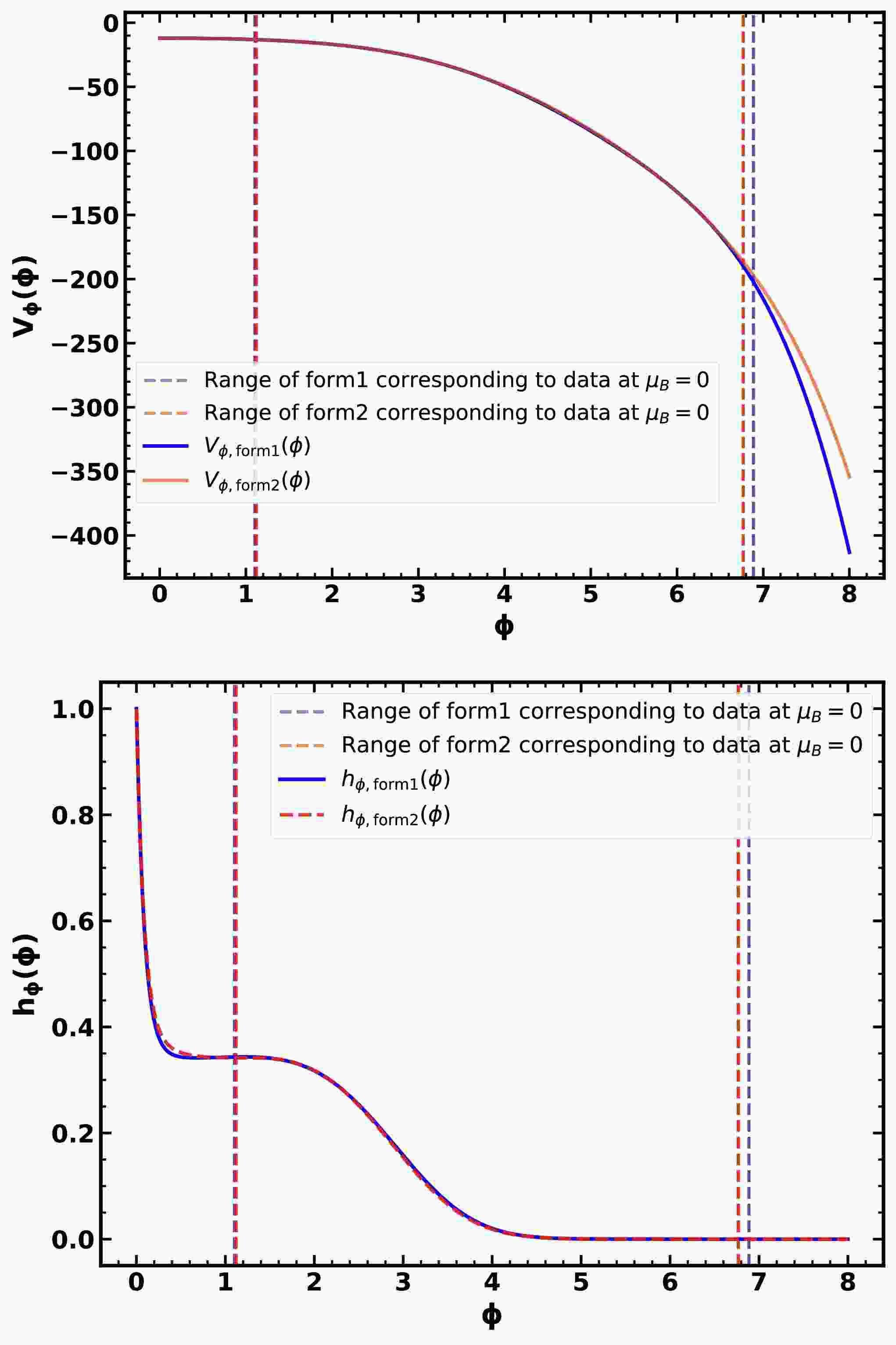
$ V_\phi(\phi) = V^{\rm E}(\Phi) $ , and$ h_{\phi}(\phi) = h(\Phi) $ .For asymptotically AdS solutions, the UV behavior of
$ V_{\phi}(\phi) $ is constrained by the scaling dimension$ \Delta_\phi $ of the operator dual to the dilaton ϕ. Expanding around$ \phi\to 0 $ , one has$ \begin{aligned}[b] V_{\phi}(\phi) &= -\frac{12}{L^{2}}+\frac{1}{2}m_{\phi}^{2}\phi^{2} +\mathcal{O}(\phi^{4}), \\ m_{\phi}^{2}L^{2} &=\Delta_{\phi}(\Delta_{\phi}-4), \end{aligned} $
(11) which is the usual AdS/CFT mass-dimension relation. In bottom-up holographic QCD,
$ \Delta_\phi $ is treated as a phenomenological UV input. It controls how fast the background departs from AdS and thus encodes the nonconformality associated with the running coupling and the trace anomaly, but it should not be identified with the perturbative QCD beta function. In this work we allow different$ \Delta_\phi $ in different calibration steps (e.g.$ \Delta_\phi=3.6 $ in the probe reconstruction of Sec. III and$ \Delta_\phi=3.8 $ in the pure-glue/back-reacted study). These choices should be viewed as effective parameters optimized for the corresponding calibration targets and temperature windows, rather than as unique predictions derived from QCD in the UV. A more quantitative running-coupling-based justification would require scanning$ \Delta_\phi $ and refitting the model functions to the thermodynamic data, which we leave for a dedicated follow-up study.According to Eqs. (3), (6), and (8), we then derive the line element of the spacetime in the Einstein frame:
$ {\rm d} s^{2}=\frac{L^2 {\rm e}^{2 A_{E}(z)}}{z^{2}}\bigg(-f(z) {\rm d} t^{2}+\frac{{\rm d} z^{2}}{f(z)}+ {\rm d} y_{1}^{2} + {\rm d} y_{2}^{2}+ {\rm d} y_{3}^{2}\bigg), $
(12) where
$ A_E(z)=A_s(z)-\sqrt{\frac{1}{6}}\phi(z). $
(13) Using the variation method, we can derive the Einstein field equations and the equations of motion of
$ A_{M} $ and ϕ from the EMD action in Eqs. (9)–(10). It should be noted that these equations are obtained by neglecting the back-reaction from the flavor sector$ S_f^s $ ; otherwise, the field equations would involve additional source terms and become significantly more complex.$ \begin{aligned}[b] & R_{M N}^{\rm E}-\frac{1}{2} g_{M N}^{\rm E} R^{\rm E}-\frac{1}{2} T_{M N}=0, \\ & \nabla_{M}\left[h_{\phi}(\phi) F^{M N}\right]=0, \\ & \partial_{M}\left[\sqrt{-g} \partial^{M} \phi\right]-\sqrt{-g}\left(\frac{\mathrm{d} V_{\phi}(\phi)}{\mathrm{d} \phi}+\frac{F_E^{2}}{4} \frac{\mathrm{d} h_{\phi}(\phi)}{\mathrm{d} \phi}\right)=0, \end{aligned} $
(14) where
$ F_E^2 \equiv{g^{\rm E}}^{MP} {g^{\rm E}}^{NQ} F_{MN} F_{PQ} $ . Where$ T_{MN} $ is the energy-momentum tensor:$ \begin{aligned}[b] T_{M N} =\; & \left(\partial_{M} \phi \right) \left(\partial_{N} \phi \right) -\frac{1}{2} g_{M N}^{\rm E} {g^{\rm E}}^{P Q}\left(\partial_{P} \phi\right) \left(\partial_{Q} \phi\right) \\ & -g_{M N}^{\rm E} V_{\phi}(\phi) +h_{\phi}(\phi) \bigg({g^{\rm E}}^{P Q} F_{M P} F_{N Q} \\ & -\frac{1}{4} g_{M N}^{\rm E} {g^{\rm E}}^{P \widetilde{P} }{g^{\rm E}}^{Q \widetilde{Q} } F_{P Q} F_{\widetilde{P} \widetilde{Q}}\bigg). \end{aligned} $
(15) We assume that all components of the vector field
$ A_{M}(z) $ vanish, except for the t-component$ A_{t}(z) $ . By substituting the metric in Eq. (12) into the equations of motion in Eq. (14), we obtain the equations of motion (EoMs) for the background fields:$ A_{t}^{\prime \prime}+A_{t}^{\prime}\left(-\frac{1}{z}+\frac{{h_{\phi}}^{\prime}}{h_{\phi}}+{A_{E}}^{\prime}\right)=0, $
(16) $ f^{\prime \prime}+f^{\prime}\left(-\frac{3}{z}+3 {A_{E}}^{\prime}\right)-\frac{{\rm e}^{-2 {A_{E}}} A_{t}^{\prime 2} z^{2} h_{\phi}}{L^2}=0, $
(17) $ A_{E}^{\prime \prime}-A_{E}^{\prime}\left(-\frac{2}{z}+A_{E}^{\prime}\right)+\frac{\phi^{\prime 2}}{6}=0, $
(18) $ \begin{aligned}[b] & \phi^{\prime \prime}+\phi^{\prime}\left(-\frac{3}{z}+\frac{f^{\prime}}{f}+3 A_{E}^{\prime}\right) \\ &\quad -\frac{L^2 {\rm e}^{2 {A_{E}}}}{z^{2} f} \frac{\mathrm{d} V_{\phi}(\phi)}{\mathrm{d} \phi} +\frac{z^{2} {\rm e}^{-2 {A_{E}}} A_{t}^{\prime 2}}{2 L^2 f} \frac{\mathrm{d} h_{\phi}(\phi)}{\mathrm{d} \phi}=0, \end{aligned} $
(19) $ \begin{aligned}[b] & A_{E}^{\prime \prime} +\frac{f^{\prime \prime}}{6 f} +A_{E}^{\prime}\left(-\frac{6}{z}+\frac{3 f^{\prime}}{2 f}\right) \\ & \quad -\frac{1}{z}\left(-\frac{4}{z}+\frac{3 f^{\prime}}{2 f}\right) +3 {A_{E}}^{\prime 2} +\frac{L^2 {\rm e}^{2 {A_{E}}} V_{\phi}}{3 z^{2} f}=0. \end{aligned} $
(20) Here and in the following, a prime denotes the derivative with respect to the holographic coordinate z. Only 4 equations are independent in the above 5 equations. So we choose Eq. (20) as a constraint and use it to check the solutions of the EoMs.
-
As discussed in Ref. [41], it is more convenient to choose the string frame when solving the vacuum expectation value of the loop operator, and it is more convenient to choose the Einstein frame to work out the gravity solution and to study the equation of state. So we apply the following Weyl transformation [42, 43] to Eq. (2):
$ \begin{array}{l} g_{M N}^{s}=\mathrm{e}^{\frac{4}{3}\Phi} g_{M N}^{E}, \end{array} $
(6) where
$ g_{MN}^{E} $ is the metric tensor in the Einstein frame. The capital letter 'E' denotes the Einstein frame. Then, Eq. (2) becomes$ \begin{aligned}[b] S^E =\;&\frac{1}{2 \kappa_{5}^{2}} \int \mathrm{d}^{5} x \sqrt{-g^E} \Big[ R^E-\frac{4}{3} {g^E}^{M N} \partial_{M} \Phi \partial_{N} \Phi \\ & -V^E(\Phi)-\frac{h(\Phi)}{4} {g^{E}}^{MP} {g^{E}}^{NQ} F_{MN} F_{PQ}\Big], \end{aligned} $
(7) where the function
$ V^E=\mathrm{e}^{\frac{4}{3}\Phi} V^{s} $ .The coefficient of the kinetic term of the dilaton field Φ is
$ \frac{4}{3} $ in Eq. (7), which is not canonical. Therefore, we define a new dilaton field ϕ:$ \phi=\sqrt{\frac{8}{3}}\Phi. $
(8) Now, the action in Eq. (7) becomes
$ S^E =\int \mathrm{d}^{5} {\mathcal{L}}^E, $
(9) where
$ \mathcal{L}^E $ is the Lagrangian density in the Einstein frame:$ \begin{aligned}[b] {\mathcal{L}}^E =\;&\frac{1}{2 \kappa_{5}^{2}} \sqrt{-g^E} \Big[ R^E-\frac{1}{2} {g^E}^{M N} \left( \partial_{M} \phi \right) \left( \partial_{N} \phi \right) \\ & -V_{\phi}(\phi)-\frac{h_{\phi}(\phi)}{4} {g^{E}}^{M \widetilde{M} }{g^{E}}^{N \widetilde{N} } F_{M N} F_{\widetilde{M} \widetilde{N}}\Big]. \end{aligned} $
(10) The function
$ V_\phi(\phi) = V^E(\Phi) $ , and$ h_{\phi}(\phi) = h(\Phi) $ .For asymptotically AdS solutions, the UV behavior of
$ V_{\phi}(\phi) $ is constrained by the scaling dimension$ \Delta_\phi $ of the operator dual to the dilaton ϕ. Expanding around$ \phi\to 0 $ , one has$ \begin{aligned}[b] V_{\phi}(\phi) &= -\frac{12}{L^{2}}+\frac{1}{2}m_{\phi}^{2}\phi^{2} +\mathcal{O}(\phi^{4}), \\ m_{\phi}^{2}L^{2} &=\Delta_{\phi}(\Delta_{\phi}-4), \end{aligned} $
(11) which is the usual AdS/CFT mass-dimension relation. In bottom-up holographic QCD,
$ \Delta_\phi $ is treated as a phenomenological UV input. It controls how fast the background departs from AdS and thus encodes the nonconformality associated with the running coupling and the trace anomaly, but it should not be identified with the perturbative QCD beta function. In this work we allow different$ \Delta_\phi $ in different calibration steps (e.g.$ \Delta_\phi=3.6 $ in the probe reconstruction of Sec. III and$ \Delta_\phi=3.8 $ in the pure-glue/back-reacted study). These choices should be viewed as effective parameters optimized for the corresponding calibration targets and temperature windows, rather than as unique predictions derived from QCD in the UV. A more quantitative running-coupling-based justification would require scanning$ \Delta_\phi $ and refitting the model functions to the thermodynamic data, which we leave for a dedicated follow-up study.According to Eqs. (3), (6), and (8), we then derive the line element of the spacetime in the Einstein frame:
$ d s^{2}=\frac{L^2 e^{2 A_{E}(z)}}{z^{2}}\bigg(-f(z) d t^{2}+\frac{d z^{2}}{f(z)}+d y_{1}^{2} +d y_{2}^{2}+d y_{3}^{2}\bigg), $
(12) where
$ A_E(z)=A_s(z)-\sqrt{\frac{1}{6}}\phi(z). $
(13) Using the variation method, we can derive the Einstein field equations and the equations of motion of
$ A_{M} $ and ϕ from the EMD action in Eqs. (9)–(10). It should be noted that these equations are obtained by neglecting the back-reaction from the flavor sector$ S_f^s $ ; otherwise, the field equations would involve additional source terms and become significantly more complex.$ \begin{aligned}[b] & R_{M N}^{E}-\frac{1}{2} g_{M N}^{E} R^{E}-\frac{1}{2} T_{M N}=0, \\ & \nabla_{M}\left[h_{\phi}(\phi) F^{M N}\right]=0, \\ & \partial_{M}\left[\sqrt{-g} \partial^{M} \phi\right]-\sqrt{-g}\left(\frac{\mathrm{d} V_{\phi}(\phi)}{\mathrm{d} \phi}+\frac{F_E^{2}}{4} \frac{\mathrm{d} h_{\phi}(\phi)}{\mathrm{d} \phi}\right)=0, \end{aligned} $
(14) Where
$ F_E^2 \equiv{g^E}^{MP} {g^E}^{NQ} F_{MN} F_{PQ} $ . Where$ T_{MN} $ is the energy-momentum tensor:$ \begin{aligned}[b] T_{M N} =\; & \left(\partial_{M} \phi \right) \left(\partial_{N} \phi \right) -\frac{1}{2} g_{M N}^{E} {g^E}^{P Q}\left(\partial_{P} \phi\right) \left(\partial_{Q} \phi\right) \\ & -g_{M N}^{E} V_{\phi}(\phi) +h_{\phi}(\phi) \bigg({g^E}^{P Q} F_{M P} F_{N Q} \\ & -\frac{1}{4} g_{M N}^{E} {g^{E}}^{P \widetilde{P} }{g^{E}}^{Q \widetilde{Q} } F_{P Q} F_{\widetilde{P} \widetilde{Q}}\bigg). \end{aligned} $
(15) We assume that all components of the vector field
$ A_{M}(z) $ vanish, except for the t-component$ A_{t}(z) $ . By substituting the metric in Eq. (12) into the equations of motion in Eq. (14), we obtain the equations of motion (EoMs) for the background fields:$ A_{t}^{\prime \prime}+A_{t}^{\prime}\left(-\frac{1}{z}+\frac{{h_{\phi}}^{\prime}}{h_{\phi}}+{A_{E}}^{\prime}\right)=0, $
(16) $ f^{\prime \prime}+f^{\prime}\left(-\frac{3}{z}+3 {A_{E}}^{\prime}\right)-\frac{e^{-2 {A_{E}}} A_{t}^{\prime 2} z^{2} h_{\phi}}{L^2}=0, $
(17) $ A_{E}^{\prime \prime}-A_{E}^{\prime}\left(-\frac{2}{z}+A_{E}^{\prime}\right)+\frac{\phi^{\prime 2}}{6}=0, $
(18) $ \begin{aligned}[b] & \phi^{\prime \prime}+\phi^{\prime}\left(-\frac{3}{z}+\frac{f^{\prime}}{f}+3 A_{E}^{\prime}\right) \\ &\quad -\frac{L^2 e^{2 {A_{E}}}}{z^{2} f} \frac{\mathrm{d} V_{\phi}(\phi)}{\mathrm{d} \phi} +\frac{z^{2} e^{-2 {A_{E}}} A_{t}^{\prime 2}}{2 L^2 f} \frac{\mathrm{d} h_{\phi}(\phi)}{\mathrm{d} \phi}=0, \end{aligned} $
(19) $ \begin{aligned}[b] & A_{E}^{\prime \prime} +\frac{f^{\prime \prime}}{6 f} +A_{E}^{\prime}\left(-\frac{6}{z}+\frac{3 f^{\prime}}{2 f}\right) \\ & \quad -\frac{1}{z}\left(-\frac{4}{z}+\frac{3 f^{\prime}}{2 f}\right) +3 {A_{E}}^{\prime 2} +\frac{L^2 e^{2 {A_{E}}} V_{\phi}}{3 z^{2} f}=0. \end{aligned} $
(20) Here and in the following, a prime denotes the derivative with respect to the holographic coordinate z. Only 4 equations are independent in the above 5 equations. So we choose Eq. (20) as a constraint and use it to check the solutions of the EoMs.
-
As discussed in Ref. [41], it is more convenient to choose the string frame when solving the vacuum expectation value of the loop operator, and it is more convenient to choose the Einstein frame to work out the gravity solution and to study the equation of state. So we apply the following Weyl transformation [42, 43] to Eq. (2):
$ \begin{array}{l} g_{M N}^{s}=\mathrm{e}^{\frac{4}{3}\Phi} g_{M N}^{\rm E}, \end{array} $
(6) where
$ g_{MN}^{\rm E} $ is the metric tensor in the Einstein frame. The capital letter 'E' denotes the Einstein frame. Then, Eq. (2) becomes$ \begin{aligned}[b] S^{\rm E} =\;&\frac{1}{2 \kappa_{5}^{2}} \int \mathrm{d}^{5} x \sqrt{-g^{\rm E}} \bigg[ R^{\rm E}-\frac{4}{3} {g^{\rm E}}^{M N} \partial_{M} \Phi \partial_{N} \Phi \\ & -V^{\rm E}(\Phi)-\frac{h(\Phi)}{4} {g^{\rm E}}^{MP} {g^{\rm E}}^{NQ} F_{MN} F_{PQ}\bigg], \end{aligned} $
(7) where the function
$ V^{\rm E}=\mathrm{e}^{\frac{4}{3}\Phi} V^{s} $ .The coefficient of the kinetic term of the dilaton field Φ is
$ {4}/{3} $ in Eq. (7), which is not canonical. Therefore, we define a new dilaton field ϕ:$ \phi=\sqrt{\frac{8}{3}}\Phi. $
(8) Now, the action in Eq. (7) becomes
$ S^{\rm E} =\int \mathrm{d}^{5} {\mathcal{L}}^{\rm E}, $
(9) where
$ \mathcal{L}^{\rm E} $ is the Lagrangian density in the Einstein frame:$ \begin{aligned}[b] {\mathcal{L}}^{\rm E} =\;&\frac{1}{2 \kappa_{5}^{2}} \sqrt{-g^{\rm E}} \Big[ R^{\rm E}-\frac{1}{2} {g^{\rm E}}^{M N} \left( \partial_{M} \phi \right) \left( \partial_{N} \phi \right) \\ & -V_{\phi}(\phi)-\frac{h_{\phi}(\phi)}{4} {g^{\rm E}}^{M \widetilde{M} }{g^{\rm E}}^{N \widetilde{N} } F_{M N} F_{\widetilde{M} \widetilde{N}}\Big]. \end{aligned} $
(10) The function
$ V_\phi(\phi) = V^{\rm E}(\Phi) $ , and$ h_{\phi}(\phi) = h(\Phi) $ .For asymptotically AdS solutions, the UV behavior of
$ V_{\phi}(\phi) $ is constrained by the scaling dimension$ \Delta_\phi $ of the operator dual to the dilaton ϕ. Expanding around$ \phi\to 0 $ , one has$ \begin{aligned}[b] V_{\phi}(\phi) &= -\frac{12}{L^{2}}+\frac{1}{2}m_{\phi}^{2}\phi^{2} +\mathcal{O}(\phi^{4}), \\ m_{\phi}^{2}L^{2} &=\Delta_{\phi}(\Delta_{\phi}-4), \end{aligned} $
(11) which is the usual AdS/CFT mass-dimension relation. In bottom-up holographic QCD,
$ \Delta_\phi $ is treated as a phenomenological UV input. It controls how fast the background departs from AdS and thus encodes the nonconformality associated with the running coupling and the trace anomaly, but it should not be identified with the perturbative QCD beta function. In this work we allow different$ \Delta_\phi $ in different calibration steps (e.g.$ \Delta_\phi=3.6 $ in the probe reconstruction of Sec. III and$ \Delta_\phi=3.8 $ in the pure-glue/back-reacted study). These choices should be viewed as effective parameters optimized for the corresponding calibration targets and temperature windows, rather than as unique predictions derived from QCD in the UV. A more quantitative running-coupling-based justification would require scanning$ \Delta_\phi $ and refitting the model functions to the thermodynamic data, which we leave for a dedicated follow-up study.According to Eqs. (3), (6), and (8), we then derive the line element of the spacetime in the Einstein frame:
$ {\rm d} s^{2}=\frac{L^2 {\rm e}^{2 A_{E}(z)}}{z^{2}}\bigg(-f(z) {\rm d} t^{2}+\frac{{\rm d} z^{2}}{f(z)}+ {\rm d} y_{1}^{2} + {\rm d} y_{2}^{2}+ {\rm d} y_{3}^{2}\bigg), $
(12) where
$ A_E(z)=A_s(z)-\sqrt{\frac{1}{6}}\phi(z). $
(13) Using the variation method, we can derive the Einstein field equations and the equations of motion of
$ A_{M} $ and ϕ from the EMD action in Eqs. (9)–(10). It should be noted that these equations are obtained by neglecting the back-reaction from the flavor sector$ S_f^s $ ; otherwise, the field equations would involve additional source terms and become significantly more complex.$ \begin{aligned}[b] & R_{M N}^{\rm E}-\frac{1}{2} g_{M N}^{\rm E} R^{\rm E}-\frac{1}{2} T_{M N}=0, \\ & \nabla_{M}\left[h_{\phi}(\phi) F^{M N}\right]=0, \\ & \partial_{M}\left[\sqrt{-g} \partial^{M} \phi\right]-\sqrt{-g}\left(\frac{\mathrm{d} V_{\phi}(\phi)}{\mathrm{d} \phi}+\frac{F_E^{2}}{4} \frac{\mathrm{d} h_{\phi}(\phi)}{\mathrm{d} \phi}\right)=0, \end{aligned} $
(14) where
$ F_E^2 \equiv{g^{\rm E}}^{MP} {g^{\rm E}}^{NQ} F_{MN} F_{PQ} $ . Where$ T_{MN} $ is the energy-momentum tensor:$ \begin{aligned}[b] T_{M N} =\; & \left(\partial_{M} \phi \right) \left(\partial_{N} \phi \right) -\frac{1}{2} g_{M N}^{\rm E} {g^{\rm E}}^{P Q}\left(\partial_{P} \phi\right) \left(\partial_{Q} \phi\right) \\ & -g_{M N}^{\rm E} V_{\phi}(\phi) +h_{\phi}(\phi) \bigg({g^{\rm E}}^{P Q} F_{M P} F_{N Q} \\ & -\frac{1}{4} g_{M N}^{\rm E} {g^{\rm E}}^{P \widetilde{P} }{g^{\rm E}}^{Q \widetilde{Q} } F_{P Q} F_{\widetilde{P} \widetilde{Q}}\bigg). \end{aligned} $
(15) We assume that all components of the vector field
$ A_{M}(z) $ vanish, except for the t-component$ A_{t}(z) $ . By substituting the metric in Eq. (12) into the equations of motion in Eq. (14), we obtain the equations of motion (EoMs) for the background fields:$ A_{t}^{\prime \prime}+A_{t}^{\prime}\left(-\frac{1}{z}+\frac{{h_{\phi}}^{\prime}}{h_{\phi}}+{A_{E}}^{\prime}\right)=0, $
(16) $ f^{\prime \prime}+f^{\prime}\left(-\frac{3}{z}+3 {A_{E}}^{\prime}\right)-\frac{{\rm e}^{-2 {A_{E}}} A_{t}^{\prime 2} z^{2} h_{\phi}}{L^2}=0, $
(17) $ A_{E}^{\prime \prime}-A_{E}^{\prime}\left(-\frac{2}{z}+A_{E}^{\prime}\right)+\frac{\phi^{\prime 2}}{6}=0, $
(18) $ \begin{aligned}[b] & \phi^{\prime \prime}+\phi^{\prime}\left(-\frac{3}{z}+\frac{f^{\prime}}{f}+3 A_{E}^{\prime}\right) \\ &\quad -\frac{L^2 {\rm e}^{2 {A_{E}}}}{z^{2} f} \frac{\mathrm{d} V_{\phi}(\phi)}{\mathrm{d} \phi} +\frac{z^{2} {\rm e}^{-2 {A_{E}}} A_{t}^{\prime 2}}{2 L^2 f} \frac{\mathrm{d} h_{\phi}(\phi)}{\mathrm{d} \phi}=0, \end{aligned} $
(19) $ \begin{aligned}[b] & A_{E}^{\prime \prime} +\frac{f^{\prime \prime}}{6 f} +A_{E}^{\prime}\left(-\frac{6}{z}+\frac{3 f^{\prime}}{2 f}\right) \\ & \quad -\frac{1}{z}\left(-\frac{4}{z}+\frac{3 f^{\prime}}{2 f}\right) +3 {A_{E}}^{\prime 2} +\frac{L^2 {\rm e}^{2 {A_{E}}} V_{\phi}}{3 z^{2} f}=0. \end{aligned} $
(20) Here and in the following, a prime denotes the derivative with respect to the holographic coordinate z. Only 4 equations are independent in the above 5 equations. So we choose Eq. (20) as a constraint and use it to check the solutions of the EoMs.
-
As discussed in Ref. [41], it is more convenient to choose the string frame when solving the vacuum expectation value of the loop operator, and it is more convenient to choose the Einstein frame to work out the gravity solution and to study the equation of state. So we apply the following Weyl transformation [42, 43] to Eq. (2):
$ \begin{array}{l} g_{M N}^{s}=\mathrm{e}^{\frac{4}{3}\Phi} g_{M N}^{\rm E}, \end{array} $
(6) where
$ g_{MN}^{\rm E} $ is the metric tensor in the Einstein frame. The capital letter 'E' denotes the Einstein frame. Then, Eq. (2) becomes$ \begin{aligned}[b] S^{\rm E} =\;&\frac{1}{2 \kappa_{5}^{2}} \int \mathrm{d}^{5} x \sqrt{-g^{\rm E}} \bigg[ R^{\rm E}-\frac{4}{3} {g^{\rm E}}^{M N} \partial_{M} \Phi \partial_{N} \Phi \\ & -V^{\rm E}(\Phi)-\frac{h(\Phi)}{4} {g^{\rm E}}^{MP} {g^{\rm E}}^{NQ} F_{MN} F_{PQ}\bigg], \end{aligned} $
(7) where the function
$ V^{\rm E}=\mathrm{e}^{\frac{4}{3}\Phi} V^{s} $ .The coefficient of the kinetic term of the dilaton field Φ is
$ {4}/{3} $ in Eq. (7), which is not canonical. Therefore, we define a new dilaton field ϕ:$ \phi=\sqrt{\frac{8}{3}}\Phi. $
(8) Now, the action in Eq. (7) becomes
$ S^{\rm E} =\int \mathrm{d}^{5} {\mathcal{L}}^{\rm E}, $
(9) where
$ \mathcal{L}^{\rm E} $ is the Lagrangian density in the Einstein frame:$ \begin{aligned}[b] {\mathcal{L}}^{\rm E} =\;&\frac{1}{2 \kappa_{5}^{2}} \sqrt{-g^{\rm E}} \Big[ R^{\rm E}-\frac{1}{2} {g^{\rm E}}^{M N} \left( \partial_{M} \phi \right) \left( \partial_{N} \phi \right) \\ & -V_{\phi}(\phi)-\frac{h_{\phi}(\phi)}{4} {g^{\rm E}}^{M \widetilde{M} }{g^{\rm E}}^{N \widetilde{N} } F_{M N} F_{\widetilde{M} \widetilde{N}}\Big]. \end{aligned} $
(10) The function
$ V_\phi(\phi) = V^{\rm E}(\Phi) $ , and$ h_{\phi}(\phi) = h(\Phi) $ .For asymptotically AdS solutions, the UV behavior of
$ V_{\phi}(\phi) $ is constrained by the scaling dimension$ \Delta_\phi $ of the operator dual to the dilaton ϕ. Expanding around$ \phi\to 0 $ , one has$ \begin{aligned}[b] V_{\phi}(\phi) &= -\frac{12}{L^{2}}+\frac{1}{2}m_{\phi}^{2}\phi^{2} +\mathcal{O}(\phi^{4}), \\ m_{\phi}^{2}L^{2} &=\Delta_{\phi}(\Delta_{\phi}-4), \end{aligned} $
(11) which is the usual AdS/CFT mass-dimension relation. In bottom-up holographic QCD,
$ \Delta_\phi $ is treated as a phenomenological UV input. It controls how fast the background departs from AdS and thus encodes the nonconformality associated with the running coupling and the trace anomaly, but it should not be identified with the perturbative QCD beta function. In this work we allow different$ \Delta_\phi $ in different calibration steps (e.g.$ \Delta_\phi=3.6 $ in the probe reconstruction of Sec. III and$ \Delta_\phi=3.8 $ in the pure-glue/back-reacted study). These choices should be viewed as effective parameters optimized for the corresponding calibration targets and temperature windows, rather than as unique predictions derived from QCD in the UV. A more quantitative running-coupling-based justification would require scanning$ \Delta_\phi $ and refitting the model functions to the thermodynamic data, which we leave for a dedicated follow-up study.According to Eqs. (3), (6), and (8), we then derive the line element of the spacetime in the Einstein frame:
$ {\rm d} s^{2}=\frac{L^2 {\rm e}^{2 A_{E}(z)}}{z^{2}}\bigg(-f(z) {\rm d} t^{2}+\frac{{\rm d} z^{2}}{f(z)}+ {\rm d} y_{1}^{2} + {\rm d} y_{2}^{2}+ {\rm d} y_{3}^{2}\bigg), $
(12) where
$ A_E(z)=A_s(z)-\sqrt{\frac{1}{6}}\phi(z). $
(13) Using the variation method, we can derive the Einstein field equations and the equations of motion of
$ A_{M} $ and ϕ from the EMD action in Eqs. (9)–(10). It should be noted that these equations are obtained by neglecting the back-reaction from the flavor sector$ S_f^s $ ; otherwise, the field equations would involve additional source terms and become significantly more complex.$ \begin{aligned}[b] & R_{M N}^{\rm E}-\frac{1}{2} g_{M N}^{\rm E} R^{\rm E}-\frac{1}{2} T_{M N}=0, \\ & \nabla_{M}\left[h_{\phi}(\phi) F^{M N}\right]=0, \\ & \partial_{M}\left[\sqrt{-g} \partial^{M} \phi\right]-\sqrt{-g}\left(\frac{\mathrm{d} V_{\phi}(\phi)}{\mathrm{d} \phi}+\frac{F_E^{2}}{4} \frac{\mathrm{d} h_{\phi}(\phi)}{\mathrm{d} \phi}\right)=0, \end{aligned} $
(14) where
$ F_E^2 \equiv{g^{\rm E}}^{MP} {g^{\rm E}}^{NQ} F_{MN} F_{PQ} $ . Where$ T_{MN} $ is the energy-momentum tensor:$ \begin{aligned}[b] T_{M N} =\; & \left(\partial_{M} \phi \right) \left(\partial_{N} \phi \right) -\frac{1}{2} g_{M N}^{\rm E} {g^{\rm E}}^{P Q}\left(\partial_{P} \phi\right) \left(\partial_{Q} \phi\right) \\ & -g_{M N}^{\rm E} V_{\phi}(\phi) +h_{\phi}(\phi) \bigg({g^{\rm E}}^{P Q} F_{M P} F_{N Q} \\ & -\frac{1}{4} g_{M N}^{\rm E} {g^{\rm E}}^{P \widetilde{P} }{g^{\rm E}}^{Q \widetilde{Q} } F_{P Q} F_{\widetilde{P} \widetilde{Q}}\bigg). \end{aligned} $
(15) We assume that all components of the vector field
$ A_{M}(z) $ vanish, except for the t-component$ A_{t}(z) $ . By substituting the metric in Eq. (12) into the equations of motion in Eq. (14), we obtain the equations of motion (EoMs) for the background fields:$ A_{t}^{\prime \prime}+A_{t}^{\prime}\left(-\frac{1}{z}+\frac{{h_{\phi}}^{\prime}}{h_{\phi}}+{A_{E}}^{\prime}\right)=0, $
(16) $ f^{\prime \prime}+f^{\prime}\left(-\frac{3}{z}+3 {A_{E}}^{\prime}\right)-\frac{{\rm e}^{-2 {A_{E}}} A_{t}^{\prime 2} z^{2} h_{\phi}}{L^2}=0, $
(17) $ A_{E}^{\prime \prime}-A_{E}^{\prime}\left(-\frac{2}{z}+A_{E}^{\prime}\right)+\frac{\phi^{\prime 2}}{6}=0, $
(18) $ \begin{aligned}[b] & \phi^{\prime \prime}+\phi^{\prime}\left(-\frac{3}{z}+\frac{f^{\prime}}{f}+3 A_{E}^{\prime}\right) \\ &\quad -\frac{L^2 {\rm e}^{2 {A_{E}}}}{z^{2} f} \frac{\mathrm{d} V_{\phi}(\phi)}{\mathrm{d} \phi} +\frac{z^{2} {\rm e}^{-2 {A_{E}}} A_{t}^{\prime 2}}{2 L^2 f} \frac{\mathrm{d} h_{\phi}(\phi)}{\mathrm{d} \phi}=0, \end{aligned} $
(19) $ \begin{aligned}[b] & A_{E}^{\prime \prime} +\frac{f^{\prime \prime}}{6 f} +A_{E}^{\prime}\left(-\frac{6}{z}+\frac{3 f^{\prime}}{2 f}\right) \\ & \quad -\frac{1}{z}\left(-\frac{4}{z}+\frac{3 f^{\prime}}{2 f}\right) +3 {A_{E}}^{\prime 2} +\frac{L^2 {\rm e}^{2 {A_{E}}} V_{\phi}}{3 z^{2} f}=0. \end{aligned} $
(20) Here and in the following, a prime denotes the derivative with respect to the holographic coordinate z. Only 4 equations are independent in the above 5 equations. So we choose Eq. (20) as a constraint and use it to check the solutions of the EoMs.
-
As mentioned earlier,
$ S_{f}^{s} $ in Eq. (1) describes the flavor part in the string frame. Here we use an improved KKSS action:$ \begin{aligned}[b] S_{f}^{s}=\;&-\int \mathrm{d}^5 x \sqrt{-g^s} {\rm e}^{-\Phi} \beta(\Phi) {\rm{Tr}} \Bigg\{ \left| D_M X \right|^2 + V_X^s(X, \Phi, F_s^2) \\ & +\frac{1}{4 g_5^2} \left( F_L^2+F_R^2 \right) \Bigg\} + S_{\text{baryons}}^{s}. \end{aligned} $
(21) where
$ D_M X=\nabla_M X-\mathrm{i} g_c A_M X $
(22) is the covariant derivative of the
$ 5 $ -dimensional scalar field X. In this work, we maintain the general polynomial form$ \begin{array}{l} \begin{aligned} V_X^s(X, \Phi, F_s^2) &= \sum_{n=1}^{2} \lambda_{2n} |X|^{2n}, \end{aligned} \end{array} $
(23) where
$\lambda_2 \equiv {M_X}_5^2 $ and$F_s^2 \equiv {g^{s}}^{MP} {g^{s}}^{NQ} F_{MN} F_{PQ}$ . The KKSS parameters$ \lambda_2 $ and$ \lambda_4 $ are precisely the coefficients entering Eq. (23), controlling the quadratic and quartic terms in$ V_X $ . Moreover,$ \lambda_2 $ is not a free parameter: it is fixed by the AdS/CFT mass-dimension relation for the bulk scalar X (see the discussion below leading to$ {M_X}_5^2=-3 $ ), while$ \lambda_4 $ will be treated phenomenologically and tuned in the back-reacted$ N_f=2 $ study. After the Weyl transformation in Eq. (6), the potential in the Einstein frame acquires an explicit dilaton dependence. In our convention,$ \begin{array}{l} V_X^{\rm E}(X, \Phi, F_E^2) =e^{\frac{4}{3}\Phi}\, V_X^s \left(X, \Phi, {\rm e}^{-\frac{8}{3}\Phi}F_E^2\right). \end{array} $
(24) where
$ F_E^2 \equiv{g^{\rm E}}^{MP} {g^{\rm E}}^{NQ} F_{MN} F_{PQ} $ . The function$ \beta(\Phi) $ controls the coupling strength between the flavor part and the EMD background, and we use the following smooth ansatz:$ \beta(\Phi)={\beta_1}\frac{\arctan \left(\beta_2 \Phi-\beta_3\right)+\dfrac{\pi}{2}}{\pi}, $
(25) where
$ (\beta_1,\beta_2,\beta_3) $ are model parameters. In this work, these parameters will be tuned in comparison with the lattice EoS in the back-reacted$ N_f=2 $ study; in particular, we will vary$ \beta_1 $ to assess the sensitivity to the overall strength of the flavor back-reaction. When writing the back-reacted equations in terms of the canonically normalized dilaton field ϕ, we use the shorthand$ \beta_{\phi}(\phi)\equiv \beta(\Phi=\sqrt{3/8}\,\phi) $ ; similarly, the Einstein-frame flavor potential may be viewed as a function of ϕ through Eq. (8). The original KKSS action is proposed in Ref. [27], and it is modified in Refs. [44−47] to describe the chiral phase transition and meson spectra.According to the AdS/CFT dictionary [26], the bulk scalar field X and the chiral gauge fields
$ A_{L,R}^M $ are dual to the relevant QCD operators at the ultraviolet (UV) boundary$ z=0 $ . The bulk scalar field X can be decomposed as$ X=\left(\frac{\chi (z)}{2}+S(x,z)\right) \mathrm{e}^{2 \mathrm{i} \pi(x,z)}, $
(26) where
$ \pi(x,z)=\pi^a(x,z) t^a $ is the pseudoscalar meson field, and$ S(x,z) $ is the scalar meson field. The field$ \chi(z) $ is related to the vacuum expectation value (VEV):$ \langle X\rangle=\frac{\chi}{2} I_{2}, $
(27) where
$ I_2 $ is the$ 2 \times 2 $ identity matrix. For the$ N_f=2 $ flavor sector studied in this work, we assume the light quark masses are degenerate, which leads to the diagonal form$ \chi \equiv \chi_u = \chi_d $ . The 5-dimensional bulk gauge field$A_{L,R}^M$ can be recombined into the vector field$ V^M $ and the axial-vector field$ A^M $ :$ \begin{aligned}[b] & V^M=\frac{1}{2}(A_L^M+A_R^M), \\& A^M=\frac{1}{2}(A_L^M-A_R^M). \end{aligned} $
(28) The field-strength tensors for the vector field and the axial-vector field are
$ \begin{aligned}[b] F_{V}^{M N} =\;&\frac{1}{2}\left(F_{L}^{M N}+F_{R}^{M N}\right) \\ =\;&\partial^{M} V^{N}-\partial^{N} V^{M}-\mathrm{i}\left[V^{M}, V^{N}\right]-\mathrm{i}\left[A^{M}, A^{N}\right], \end{aligned} $
(29) $ \begin{aligned}[b] F_{A}^{M N} =\;&\frac{1}{2}\left(F_{L}^{M N}-F_{R}^{M N}\right) \\ =\;&\partial^{M} A^{N}-\partial^{N} A^{M}-\mathrm{i}\left[V^{M}, A^{N}\right]-\mathrm{i}\left[A^{M}, V^{N}\right]. \end{aligned} $
(30) According to the mass-dimension relationship
$ M^2= (\Delta-p)(\Delta+p-4) $ and given$ \Delta=3 $ and$ p=0 $ , the 5-dimensional mass squared of the bulk field X is$ {M_X}_5^2=-3 $ .The action
$ S_{f}^{s} $ that describes the flavor part can be decomposed as$ S_{f}^{s}=S_{\chi}^{s}+S_{\text{mesons}}^{s}+S_{\text{baryons}}^{s}, $
(31) where
$ \begin{aligned}[b] S_{\chi}^{s}=\;&- \int \mathrm{d}^5 x \sqrt{-g^s}\,\mathrm{e}^{-\Phi}\,\beta(\Phi) \bigg\{ \frac{1}{2} \left| \partial_M \chi -\mathrm{i} g_c A_M \chi \right|^2 \\ & +{\rm{Tr}} \left[V_X^s \left(\langle X\rangle,\Phi,F_s^2\right)\right] \bigg\}. \end{aligned} $
(32) After the Weyl transformation in Eq. (6), the corresponding action in the Einstein frame can be written as:
$ \begin{aligned}[b] S_{\chi}^{\rm E} =\;&-\int \mathrm{d}^5 x \sqrt{-g^{\rm E}}\,\mathrm{e}^{\Phi}\,\beta(\Phi) \bigg\{\frac{1}{2} \left| \partial_M \chi -\mathrm{i} g_c A_M \chi \right|_{E}^{2} \\ & +{\rm{Tr}} \left[V_X^{\rm E} \left(\langle X\rangle,\Phi,F_E^2\right)\right]\bigg\}, \end{aligned} $
(33) where
$ \left|\cdots\right|_{E}^{2}\equiv{g^{\rm E}}^{MN}(\cdots)^\dagger(\cdots) $ and$ V_X^{\rm E} $ is defined in Eq. (24). Equation (33) is the action for the thermodynamic VEV$ \chi(z) $ . The$ 5 $ -dimensional fields dual to the meson and baryon towers are treated as perturbations around this background. The contributions from$ S_{\text{mesons}}^{s} $ and$ S_{\text{baryons}}^{s} $ to the thermodynamics are expected to be subleading compared to that from$ S_{\chi}^{s} $ , and thus we neglect them in the thermodynamic calculation in this article. -
As mentioned earlier,
$ S_{f}^{s} $ in Eq. (1) describes the flavor part in the string frame. Here we use an improved KKSS action:$ \begin{aligned}[b] S_{f}^{s}=\;&-\int \mathrm{d}^5 x \sqrt{-g^s} e^{-\Phi} \beta(\Phi) \times {\rm{Tr}} \Bigg\{ \left| D_M X \right|^2 + V_X^s(X, \Phi, F_s^2) \\ & +\frac{1}{4 g_5^2} \left( F_L^2+F_R^2 \right) \Bigg\} + S_{\text{baryons}}^{s}. \end{aligned} $
(21) where
$ D_M X=\nabla_M X-\mathrm{i} g_c A_M X $
(22) is the covariant derivative of the
$ 5 $ -dimensional scalar field X. In this work, we maintain the general polynomial form$ \begin{array}{l} \begin{aligned} V_X^s(X, \Phi, F_s^2) &= \sum_{n=1}^{2} \lambda_{2n} |X|^{2n}, \end{aligned} \end{array} $
(23) the KKSS parameters
$ \lambda_2 $ and$ \lambda_4 $ are precisely the coefficients entering Eq. (23), controlling the quadratic and quartic terms in$ V_X $ . Moreover,$ \lambda_2 $ is not a free parameter: it is fixed by the AdS/CFT mass-dimension relation for the bulk scalar X (see the discussion below leading to$ {M_X}_5^2=-3 $ ), while$ \lambda_4 $ will be treated phenomenologically and tuned in the back-reacted$ N_f=2 $ study. After the Weyl transformation in Eq. (6), the potential in the Einstein frame acquires an explicit dilaton dependence. In our convention,$ \begin{array}{l} V_X^E(X, \Phi, F_E^2) =e^{\frac{4}{3}\Phi}\, V_X^s \left(X, \Phi, e^{-\frac{8}{3}\Phi}F_E^2\right). \end{array} $
(24) where
$ F_E^2 \equiv{g^{E}}^{MP} {g^{E}}^{NQ} F_{MN} F_{PQ} $ . The function$ \beta(\Phi) $ controls the coupling strength between the flavor part and the EMD background, and we use the following smooth ansatz:$ \beta(\Phi)={\beta_1}\frac{\arctan \left(\beta_2 \Phi-\beta_3\right)+\dfrac{\pi}{2}}{\pi}, $
(25) where
$ (\beta_1,\beta_2,\beta_3) $ are model parameters. In this work, these parameters will be tuned in comparison with the lattice EoS in the back-reacted$ N_f=2 $ study; in particular, we will vary$ \beta_1 $ to assess the sensitivity to the overall strength of the flavor back-reaction. When writing the back-reacted equations in terms of the canonically normalized dilaton field ϕ, we use the shorthand$ \beta_{\phi}(\phi)\equiv \beta(\Phi=\sqrt{3/8}\,\phi) $ ; similarly, the Einstein-frame flavor potential may be viewed as a function of ϕ through Eq. (8). The original KKSS action is proposed in Ref. [27], and it is modified in Refs. [44−47] to describe the chiral phase transition and meson spectra.According to the AdS/CFT dictionary [26], the bulk scalar field X and the chiral gauge fields
$ A_{L,R}^M $ are dual to the relevant QCD operators at the ultraviolet (UV) boundary$ z=0 $ . The bulk scalar field X can be decomposed as$ X=\left(\frac{\chi (z)}{2}+S(x,z)\right) \mathrm{e}^{2 \mathrm{i} \pi(x,z)}, $
(26) where
$ \pi(x,z)=\pi^a(x,z) t^a $ is the pseudoscalar meson field, and$ S(x,z) $ is the scalar meson field. The field$ \chi(z) $ is related to the vacuum expectation value (VEV):$ \langle X\rangle=\frac{\chi}{2} I_{2}, $
(27) where
$ I_2 $ is the$ 2 \times 2 $ identity matrix. For the$ N_f=2 $ flavor sector studied in this work, we assume the light quark masses are degenerate, which leads to the diagonal form$ \chi \equiv \chi_u = \chi_d $ . The 5-dimensional bulk gauge field$A_{L,R}^M$ can be recombined into the vector field$ V^M $ and the axial-vector field$ A^M $ :$ \begin{aligned}[b] & V^M=\frac{1}{2}(A_L^M+A_R^M), \\& A^M=\frac{1}{2}(A_L^M-A_R^M). \end{aligned} $
(28) The field-strength tensors for the vector field and the axial-vector field are
$ \begin{aligned}[b] F_{V}^{M N} =\;&\frac{1}{2}\left(F_{L}^{M N}+F_{R}^{M N}\right) \\ =\;&\partial^{M} V^{N}-\partial^{N} V^{M}-\mathrm{i}\left[V^{M}, V^{N}\right]-\mathrm{i}\left[A^{M}, A^{N}\right], \end{aligned} $
(29) $ \begin{aligned}[b] F_{A}^{M N} =\;&\frac{1}{2}\left(F_{L}^{M N}-F_{R}^{M N}\right) \\ =\;&\partial^{M} A^{N}-\partial^{N} A^{M}-\mathrm{i}\left[V^{M}, A^{N}\right]-\mathrm{i}\left[A^{M}, V^{N}\right]. \end{aligned} $
(30) According to the mass-dimension relationship
$ M^2=(\Delta-p)(\Delta+p-4) $ and given$ \Delta=3 $ and$ p=0 $ , the 5-dimensional mass squared of the bulk field X is$ {M_X}_5^2=-3 $ .The action
$ S_{f}^{s} $ that describes the flavor part can be decomposed as$ S_{f}^{s}=S_{\chi}^{s}+S_{\text{mesons}}^{s}+S_{\text{baryons}}^{s}, $
(31) where
$ \begin{aligned}[b] S_{\chi}^{s}=\;&- \int \mathrm{d}^5 x \sqrt{-g^s}\,\mathrm{e}^{-\Phi}\,\beta(\Phi) \bigg\{ \frac{1}{2} \left| \partial_M \chi -\mathrm{i} g_c A_M \chi \right|^2 \\ & +{\rm{Tr}} \left[V_X^s \left(\langle X\rangle,\Phi,F_s^2\right)\right] \bigg\} \end{aligned} $
(32) After the Weyl transformation in Eq. (6), the corresponding action in the Einstein frame can be written as:
$ \begin{aligned}[b] S_{\chi}^{E} =\;&-\int \mathrm{d}^5 x \sqrt{-g^{E}}\,\mathrm{e}^{\Phi}\,\beta(\Phi) \bigg\{\frac{1}{2} \left| \partial_M \chi -\mathrm{i} g_c A_M \chi \right|_{E}^{2} \\ & +{\rm{Tr}} \left[V_X^E \left(\langle X\rangle,\Phi,F_E^2\right)\right]\bigg\}, \end{aligned} $
(33) where
$ \left|\cdots\right|_{E}^{2}\equiv{g^E}^{MN}(\cdots)^\dagger(\cdots) $ and$ V_X^E $ is defined in Eq. (24). Equation (33) is the action for the thermodynamic VEV$ \chi(z) $ . The$ 5 $ -dimensional fields dual to the meson and baryon towers are treated as perturbations around this background. The contributions from$ S_{\text{mesons}}^{s} $ and$ S_{\text{baryons}}^{s} $ to the thermodynamics are expected to be subleading compared to that from$ S_{\chi}^{s} $ , and thus we neglect them in the thermodynamic calculation in this article. -
As mentioned earlier,
$ S_{f}^{s} $ in Eq. (1) describes the flavor part in the string frame. Here we use an improved KKSS action:$ \begin{aligned}[b] S_{f}^{s}=\;&-\int \mathrm{d}^5 x \sqrt{-g^s} {\rm e}^{-\Phi} \beta(\Phi) {\rm{Tr}} \Bigg\{ \left| D_M X \right|^2 + V_X^s(X, \Phi, F_s^2) \\ & +\frac{1}{4 g_5^2} \left( F_L^2+F_R^2 \right) \Bigg\} + S_{\text{baryons}}^{s}. \end{aligned} $
(21) where
$ D_M X=\nabla_M X-\mathrm{i} g_c A_M X $
(22) is the covariant derivative of the
$ 5 $ -dimensional scalar field X. In this work, we maintain the general polynomial form$ \begin{array}{l} \begin{aligned} V_X^s(X, \Phi, F_s^2) &= \sum_{n=1}^{2} \lambda_{2n} |X|^{2n}, \end{aligned} \end{array} $
(23) where
$\lambda_2 \equiv {M_X}_5^2 $ and$F_s^2 \equiv {g^{s}}^{MP} {g^{s}}^{NQ} F_{MN} F_{PQ}$ . The KKSS parameters$ \lambda_2 $ and$ \lambda_4 $ are precisely the coefficients entering Eq. (23), controlling the quadratic and quartic terms in$ V_X $ . Moreover,$ \lambda_2 $ is not a free parameter: it is fixed by the AdS/CFT mass-dimension relation for the bulk scalar X (see the discussion below leading to$ {M_X}_5^2=-3 $ ), while$ \lambda_4 $ will be treated phenomenologically and tuned in the back-reacted$ N_f=2 $ study. After the Weyl transformation in Eq. (6), the potential in the Einstein frame acquires an explicit dilaton dependence. In our convention,$ \begin{array}{l} V_X^{\rm E}(X, \Phi, F_E^2) =e^{\frac{4}{3}\Phi}\, V_X^s \left(X, \Phi, {\rm e}^{-\frac{8}{3}\Phi}F_E^2\right). \end{array} $
(24) where
$ F_E^2 \equiv{g^{\rm E}}^{MP} {g^{\rm E}}^{NQ} F_{MN} F_{PQ} $ . The function$ \beta(\Phi) $ controls the coupling strength between the flavor part and the EMD background, and we use the following smooth ansatz:$ \beta(\Phi)={\beta_1}\frac{\arctan \left(\beta_2 \Phi-\beta_3\right)+\dfrac{\pi}{2}}{\pi}, $
(25) where
$ (\beta_1,\beta_2,\beta_3) $ are model parameters. In this work, these parameters will be tuned in comparison with the lattice EoS in the back-reacted$ N_f=2 $ study; in particular, we will vary$ \beta_1 $ to assess the sensitivity to the overall strength of the flavor back-reaction. When writing the back-reacted equations in terms of the canonically normalized dilaton field ϕ, we use the shorthand$ \beta_{\phi}(\phi)\equiv \beta(\Phi=\sqrt{3/8}\,\phi) $ ; similarly, the Einstein-frame flavor potential may be viewed as a function of ϕ through Eq. (8). The original KKSS action is proposed in Ref. [27], and it is modified in Refs. [44−47] to describe the chiral phase transition and meson spectra.According to the AdS/CFT dictionary [26], the bulk scalar field X and the chiral gauge fields
$ A_{L,R}^M $ are dual to the relevant QCD operators at the ultraviolet (UV) boundary$ z=0 $ . The bulk scalar field X can be decomposed as$ X=\left(\frac{\chi (z)}{2}+S(x,z)\right) \mathrm{e}^{2 \mathrm{i} \pi(x,z)}, $
(26) where
$ \pi(x,z)=\pi^a(x,z) t^a $ is the pseudoscalar meson field, and$ S(x,z) $ is the scalar meson field. The field$ \chi(z) $ is related to the vacuum expectation value (VEV):$ \langle X\rangle=\frac{\chi}{2} I_{2}, $
(27) where
$ I_2 $ is the$ 2 \times 2 $ identity matrix. For the$ N_f=2 $ flavor sector studied in this work, we assume the light quark masses are degenerate, which leads to the diagonal form$ \chi \equiv \chi_u = \chi_d $ . The 5-dimensional bulk gauge field$A_{L,R}^M$ can be recombined into the vector field$ V^M $ and the axial-vector field$ A^M $ :$ \begin{aligned}[b] & V^M=\frac{1}{2}(A_L^M+A_R^M), \\& A^M=\frac{1}{2}(A_L^M-A_R^M). \end{aligned} $
(28) The field-strength tensors for the vector field and the axial-vector field are
$ \begin{aligned}[b] F_{V}^{M N} =\;&\frac{1}{2}\left(F_{L}^{M N}+F_{R}^{M N}\right) \\ =\;&\partial^{M} V^{N}-\partial^{N} V^{M}-\mathrm{i}\left[V^{M}, V^{N}\right]-\mathrm{i}\left[A^{M}, A^{N}\right], \end{aligned} $
(29) $ \begin{aligned}[b] F_{A}^{M N} =\;&\frac{1}{2}\left(F_{L}^{M N}-F_{R}^{M N}\right) \\ =\;&\partial^{M} A^{N}-\partial^{N} A^{M}-\mathrm{i}\left[V^{M}, A^{N}\right]-\mathrm{i}\left[A^{M}, V^{N}\right]. \end{aligned} $
(30) According to the mass-dimension relationship
$ M^2= (\Delta-p)(\Delta+p-4) $ and given$ \Delta=3 $ and$ p=0 $ , the 5-dimensional mass squared of the bulk field X is$ {M_X}_5^2=-3 $ .The action
$ S_{f}^{s} $ that describes the flavor part can be decomposed as$ S_{f}^{s}=S_{\chi}^{s}+S_{\text{mesons}}^{s}+S_{\text{baryons}}^{s}, $
(31) where
$ \begin{aligned}[b] S_{\chi}^{s}=\;&- \int \mathrm{d}^5 x \sqrt{-g^s}\,\mathrm{e}^{-\Phi}\,\beta(\Phi) \bigg\{ \frac{1}{2} \left| \partial_M \chi -\mathrm{i} g_c A_M \chi \right|^2 \\ & +{\rm{Tr}} \left[V_X^s \left(\langle X\rangle,\Phi,F_s^2\right)\right] \bigg\}. \end{aligned} $
(32) After the Weyl transformation in Eq. (6), the corresponding action in the Einstein frame can be written as:
$ \begin{aligned}[b] S_{\chi}^{\rm E} =\;&-\int \mathrm{d}^5 x \sqrt{-g^{\rm E}}\,\mathrm{e}^{\Phi}\,\beta(\Phi) \bigg\{\frac{1}{2} \left| \partial_M \chi -\mathrm{i} g_c A_M \chi \right|_{E}^{2} \\ & +{\rm{Tr}} \left[V_X^{\rm E} \left(\langle X\rangle,\Phi,F_E^2\right)\right]\bigg\}, \end{aligned} $
(33) where
$ \left|\cdots\right|_{E}^{2}\equiv{g^{\rm E}}^{MN}(\cdots)^\dagger(\cdots) $ and$ V_X^{\rm E} $ is defined in Eq. (24). Equation (33) is the action for the thermodynamic VEV$ \chi(z) $ . The$ 5 $ -dimensional fields dual to the meson and baryon towers are treated as perturbations around this background. The contributions from$ S_{\text{mesons}}^{s} $ and$ S_{\text{baryons}}^{s} $ to the thermodynamics are expected to be subleading compared to that from$ S_{\chi}^{s} $ , and thus we neglect them in the thermodynamic calculation in this article. -
As mentioned earlier,
$ S_{f}^{s} $ in Eq. (1) describes the flavor part in the string frame. Here we use an improved KKSS action:$ \begin{aligned}[b] S_{f}^{s}=\;&-\int \mathrm{d}^5 x \sqrt{-g^s} {\rm e}^{-\Phi} \beta(\Phi) {\rm{Tr}} \Bigg\{ \left| D_M X \right|^2 + V_X^s(X, \Phi, F_s^2) \\ & +\frac{1}{4 g_5^2} \left( F_L^2+F_R^2 \right) \Bigg\} + S_{\text{baryons}}^{s}. \end{aligned} $
(21) where
$ D_M X=\nabla_M X-\mathrm{i} g_c A_M X $
(22) is the covariant derivative of the
$ 5 $ -dimensional scalar field X. In this work, we maintain the general polynomial form$ \begin{array}{l} \begin{aligned} V_X^s(X, \Phi, F_s^2) &= \sum_{n=1}^{2} \lambda_{2n} |X|^{2n}, \end{aligned} \end{array} $
(23) where
$\lambda_2 \equiv {M_X}_5^2 $ and$F_s^2 \equiv {g^{s}}^{MP} {g^{s}}^{NQ} F_{MN} F_{PQ}$ . The KKSS parameters$ \lambda_2 $ and$ \lambda_4 $ are precisely the coefficients entering Eq. (23), controlling the quadratic and quartic terms in$ V_X $ . Moreover,$ \lambda_2 $ is not a free parameter: it is fixed by the AdS/CFT mass-dimension relation for the bulk scalar X (see the discussion below leading to$ {M_X}_5^2=-3 $ ), while$ \lambda_4 $ will be treated phenomenologically and tuned in the back-reacted$ N_f=2 $ study. After the Weyl transformation in Eq. (6), the potential in the Einstein frame acquires an explicit dilaton dependence. In our convention,$ \begin{array}{l} V_X^{\rm E}(X, \Phi, F_E^2) =e^{\frac{4}{3}\Phi}\, V_X^s \left(X, \Phi, {\rm e}^{-\frac{8}{3}\Phi}F_E^2\right). \end{array} $
(24) where
$ F_E^2 \equiv{g^{\rm E}}^{MP} {g^{\rm E}}^{NQ} F_{MN} F_{PQ} $ . The function$ \beta(\Phi) $ controls the coupling strength between the flavor part and the EMD background, and we use the following smooth ansatz:$ \beta(\Phi)={\beta_1}\frac{\arctan \left(\beta_2 \Phi-\beta_3\right)+\dfrac{\pi}{2}}{\pi}, $
(25) where
$ (\beta_1,\beta_2,\beta_3) $ are model parameters. In this work, these parameters will be tuned in comparison with the lattice EoS in the back-reacted$ N_f=2 $ study; in particular, we will vary$ \beta_1 $ to assess the sensitivity to the overall strength of the flavor back-reaction. When writing the back-reacted equations in terms of the canonically normalized dilaton field ϕ, we use the shorthand$ \beta_{\phi}(\phi)\equiv \beta(\Phi=\sqrt{3/8}\,\phi) $ ; similarly, the Einstein-frame flavor potential may be viewed as a function of ϕ through Eq. (8). The original KKSS action is proposed in Ref. [27], and it is modified in Refs. [44−47] to describe the chiral phase transition and meson spectra.According to the AdS/CFT dictionary [26], the bulk scalar field X and the chiral gauge fields
$ A_{L,R}^M $ are dual to the relevant QCD operators at the ultraviolet (UV) boundary$ z=0 $ . The bulk scalar field X can be decomposed as$ X=\left(\frac{\chi (z)}{2}+S(x,z)\right) \mathrm{e}^{2 \mathrm{i} \pi(x,z)}, $
(26) where
$ \pi(x,z)=\pi^a(x,z) t^a $ is the pseudoscalar meson field, and$ S(x,z) $ is the scalar meson field. The field$ \chi(z) $ is related to the vacuum expectation value (VEV):$ \langle X\rangle=\frac{\chi}{2} I_{2}, $
(27) where
$ I_2 $ is the$ 2 \times 2 $ identity matrix. For the$ N_f=2 $ flavor sector studied in this work, we assume the light quark masses are degenerate, which leads to the diagonal form$ \chi \equiv \chi_u = \chi_d $ . The 5-dimensional bulk gauge field$A_{L,R}^M$ can be recombined into the vector field$ V^M $ and the axial-vector field$ A^M $ :$ \begin{aligned}[b] & V^M=\frac{1}{2}(A_L^M+A_R^M), \\& A^M=\frac{1}{2}(A_L^M-A_R^M). \end{aligned} $
(28) The field-strength tensors for the vector field and the axial-vector field are
$ \begin{aligned}[b] F_{V}^{M N} =\;&\frac{1}{2}\left(F_{L}^{M N}+F_{R}^{M N}\right) \\ =\;&\partial^{M} V^{N}-\partial^{N} V^{M}-\mathrm{i}\left[V^{M}, V^{N}\right]-\mathrm{i}\left[A^{M}, A^{N}\right], \end{aligned} $
(29) $ \begin{aligned}[b] F_{A}^{M N} =\;&\frac{1}{2}\left(F_{L}^{M N}-F_{R}^{M N}\right) \\ =\;&\partial^{M} A^{N}-\partial^{N} A^{M}-\mathrm{i}\left[V^{M}, A^{N}\right]-\mathrm{i}\left[A^{M}, V^{N}\right]. \end{aligned} $
(30) According to the mass-dimension relationship
$ M^2= (\Delta-p)(\Delta+p-4) $ and given$ \Delta=3 $ and$ p=0 $ , the 5-dimensional mass squared of the bulk field X is$ {M_X}_5^2=-3 $ .The action
$ S_{f}^{s} $ that describes the flavor part can be decomposed as$ S_{f}^{s}=S_{\chi}^{s}+S_{\text{mesons}}^{s}+S_{\text{baryons}}^{s}, $
(31) where
$ \begin{aligned}[b] S_{\chi}^{s}=\;&- \int \mathrm{d}^5 x \sqrt{-g^s}\,\mathrm{e}^{-\Phi}\,\beta(\Phi) \bigg\{ \frac{1}{2} \left| \partial_M \chi -\mathrm{i} g_c A_M \chi \right|^2 \\ & +{\rm{Tr}} \left[V_X^s \left(\langle X\rangle,\Phi,F_s^2\right)\right] \bigg\}. \end{aligned} $
(32) After the Weyl transformation in Eq. (6), the corresponding action in the Einstein frame can be written as:
$ \begin{aligned}[b] S_{\chi}^{\rm E} =\;&-\int \mathrm{d}^5 x \sqrt{-g^{\rm E}}\,\mathrm{e}^{\Phi}\,\beta(\Phi) \bigg\{\frac{1}{2} \left| \partial_M \chi -\mathrm{i} g_c A_M \chi \right|_{E}^{2} \\ & +{\rm{Tr}} \left[V_X^{\rm E} \left(\langle X\rangle,\Phi,F_E^2\right)\right]\bigg\}, \end{aligned} $
(33) where
$ \left|\cdots\right|_{E}^{2}\equiv{g^{\rm E}}^{MN}(\cdots)^\dagger(\cdots) $ and$ V_X^{\rm E} $ is defined in Eq. (24). Equation (33) is the action for the thermodynamic VEV$ \chi(z) $ . The$ 5 $ -dimensional fields dual to the meson and baryon towers are treated as perturbations around this background. The contributions from$ S_{\text{mesons}}^{s} $ and$ S_{\text{baryons}}^{s} $ to the thermodynamics are expected to be subleading compared to that from$ S_{\chi}^{s} $ , and thus we neglect them in the thermodynamic calculation in this article. -
In the general case where the back-reaction of the flavor sector is considered, the fields
$ \{A_t, f, A_E, \phi, X\} $ are solved simultaneously as a coupled system. By varying the total action$ S_{total}^E = S_{EMD}^E + S_{\chi}^E $ , we can derive the complete Einstein field equations and the equations of motion for the gauge field$ A_M $ , the dilaton ϕ, and the scalar field X. Here, we focus on the thermodynamic background and only consider the contribution from the vacuum expectation value (VEV)$ \chi(z) $ , while the fluctuations corresponding to meson and baryon excitations are neglected in the coupled equations. In tensor form, these equations are given by:$ \begin{aligned}[b] & \frac{1}{16\pi G_5} \left[ R_{M N}^{E}-\frac{1}{2} g_{M N}^{E} R^{E} - \frac{1}{2} T_{MN}^{EMD} \right] \\ & \quad - \frac{1}{2} e^{\sqrt{3/8}\phi}\beta_{\phi}(\phi) T_{MN}^{\chi} = 0, \end{aligned} $
(34) $ \begin{aligned}[b] & \partial_{M}\bigg[\sqrt{-g} \bigg( \frac{h_{\phi}}{16\pi G_5} + 4 e^{\sqrt{3/8}\phi}\beta_{\phi}(\phi)\, \frac{\partial}{\partial F_E^2} \\&\quad\times\Big\{{\rm{Tr}} \Big[ V_X^E(\langle X \rangle, \phi, F_E^2) \Big]\Big\} \bigg) \times {g^E}^{MP} {g^E}^{NQ} F_{PQ} \bigg] \\ & \quad - 2 \sqrt{-g} e^{\sqrt{3/8}\phi} \beta_{\phi}(\phi) g_c^2 {g^E}^{NM} A_M {\rm{Tr}} \Big[ \langle X \rangle^\dagger \langle X \rangle \Big] = 0, \end{aligned} $
(35) $ \begin{aligned}[b] & \partial_{M}\left[\frac{\sqrt{-g}}{16\pi G_5} {g^E}^{MN} \partial_{N} \phi\right] \\&\quad- \frac{1}{16\pi G_5} \left( \sqrt{-g} \frac{\mathrm{d} V_{\phi}}{\mathrm{d} \phi} + \sqrt{-g} \frac{F_E^{2}}{4} \frac{\mathrm{d} h_{\phi}}{\mathrm{d} \phi} \right) \\ & \quad - \frac{\partial}{\partial \phi} \Big\{ \sqrt{-g}\,e^{\sqrt{3/8}\phi}\beta_{\phi}(\phi)\, {\rm{Tr}} \Big[ {g^E}^{PQ} D_P \langle X \rangle^\dagger D_Q \langle X \rangle \\ & \quad + V_X^E(\langle X \rangle, \phi, F_E^2) \Big] \Big\} = 0, \\[-10pt]\end{aligned} $
(36) $ \begin{aligned}[b] & D_M \Big( \sqrt{-g}\,e^{\sqrt{3/8}\phi}\beta_{\phi}(\phi) {g^E}^{MN} D_N \langle X \rangle \Big) \\ & \quad - \sqrt{-g}\,e^{\sqrt{3/8}\phi}\beta_{\phi}(\phi)\, \frac{\partial}{\partial \langle X \rangle^\dagger} \Big\{{\rm{Tr}} \Big[ V_X^E(\langle X \rangle, \phi, F_E^2) \Big]\Big\} = 0, \end{aligned} $
(37) Where
$ T_{MN}^{EMD} $ is defined in Eq. (15), the general flavor energy-momentum tensor is defined using the trace operator:$ \begin{aligned}[b] T_{MN}^{\chi} =\; & {\rm{Tr}} \Big[ \left( D_M \langle X \rangle \right)^\dagger D_N \langle X \rangle+\left( D_N \langle X \rangle \right)^\dagger D_M \langle X \rangle \\ & \quad - g_{MN}^E \Big( {g^E}^{PQ} \left( D_P \langle X \rangle \right)^\dagger D_Q \langle X \rangle + V_X^E(\langle X \rangle, \phi, F_E^2) \Big) \Big] \\ & \quad+ 4 \frac{\partial \{ {\rm{Tr}} [ V_X^E(\langle X \rangle, \phi, F_E^2) ] \}}{\partial F_E^2} {g^E}^{PQ} F_{MP} F_{NQ}. \end{aligned} $
(38) After substituting the metric ansatz into the above tensor equations, and following the style of Eqs. (16)–(19), we obtain the following complete set of back-reacted equations of motion for
$ N_f=2 $ flavors in the Einstein frame. To simplify the expressions, we define the effective gauge kinetic function as follows:$ \mathcal{K}(z) \equiv\, h_{\phi} + 64\pi G_5 e^{\sqrt{3/8}\phi}\beta_{\phi}(\phi) \frac{\partial}{\partial F_E^2} {\rm{Tr}} \Big[ V_X^E(\langle X \rangle, \phi, F_E^2) \Big]. $
(39) The coupled equations are given by:
$\begin{aligned}[b]& A_{t}^{\prime \prime}+A_{t}^{\prime}\left(-\frac{1}{z} + A_{E}^{\prime} + \frac{\mathcal{K}'}{\mathcal{K}}\right) \\&\quad - \frac{16\pi G_5 L^2 e^{2A_E+\sqrt{3/8}\phi} \beta_{\phi}(\phi) g_c^2 A_t \chi^2}{z^2 f \mathcal{K}} = 0,\end{aligned} $
(40) $ \begin{aligned}[b] & f^{\prime \prime}+f^{\prime}\left(-\frac{3}{z}+3 {A_{E}}^{\prime}\right) \\ &\quad - \frac{16\pi G_5 e^{\sqrt{3/8}\phi}\beta_{\phi}(\phi) g_c^2 A_t^2 \chi^2}{f} - \frac{z^{2} e^{-2 {A_{E}}} A_{t}^{\prime 2}}{L^2} \mathcal{K} = 0, \end{aligned} $
(41) $ \begin{aligned}[b] & A_{E}^{\prime \prime}-A_{E}^{\prime}\left(-\frac{2}{z}+A_{E}^{\prime}\right)+\frac{\phi^{\prime 2}}{6} \end{aligned} $
$ \begin{aligned}[b] + \frac{8\pi G_5 e^{\sqrt{3/8}\phi}\beta_{\phi}(\phi) g_c^2 A_t^2 \chi^2}{3 f^2} + \frac{8\pi G_5 e^{\sqrt{3/8}\phi}\beta_{\phi}(\phi) \chi^{\prime 2}}{3} = 0, \end{aligned} $
(42) $ \begin{aligned}[b] & \phi^{\prime \prime}+\phi^{\prime}\left(-\frac{3}{z} + \frac{f^{\prime}}{f} + 3 A_{E}^{\prime}\right) - \frac{L^2 e^{2 {A_{E}}}}{z^{2} f} \frac{\mathrm{d} V_{\phi}}{\mathrm{d} \phi} \\ & \quad + \frac{z^{2} A_{t}^{\prime 2}}{2 L^2 e^{2 {A_{E}}} f} \frac{\mathrm{d} h_{\phi}}{\mathrm{d} \phi} - 8\pi G_5 \left( \chi^{\prime 2} - \frac{g_c^2 A_t^2 \chi^2}{f^2} \right) \frac{\mathrm{d} [e^{\sqrt{3/8}\phi}\beta_{\phi}(\phi)]}{\mathrm{d} \phi} \\ & \quad - \frac{16\pi G_5 L^2 e^{2 {A_{E}}}}{z^{2} f} \frac{\partial \{ e^{\sqrt{3/8}\phi}\beta_{\phi}(\phi) {\rm{Tr}}[ V_X^E(\langle X \rangle, \phi, F_E^2) ] \}}{\partial \phi} = 0, \end{aligned} $
(43) $ \begin{aligned}[b] & \chi'' + \chi' \left[ 3A_E' - \frac{3}{z} + \frac{f'}{f} + \sqrt{\frac{3}{8}}\,\phi' + \frac{\phi'}{\beta_{\phi}(\phi)} \frac{\mathrm{d} \beta_{\phi}(\phi)}{\mathrm{d} \phi} \right] \\ & \quad + \frac{g_c^2 A_t^2 \chi}{f^2} - \frac{L^2 e^{2 A_E}}{z^2 f} \frac{\partial \{ {\rm{Tr}}[ V_X^E(\langle X \rangle, \phi, F_E^2) ] \}}{\partial \chi} = 0, \end{aligned} $
(44) $ \begin{aligned}[b] & A_{E}^{\prime \prime} +\frac{f^{\prime \prime}}{6 f} + A_{E}^{\prime}\left(-\frac{6}{z}+\frac{3 f^{\prime}}{2 f}\right) -\frac{1}{z}\left(-\frac{4}{z}+\frac{3 f^{\prime}}{2 f}\right) \\ & \quad + 3 {A_{E}}^{\prime 2} - \frac{8\pi G_5 e^{\sqrt{3/8}\phi}\beta_{\phi}(\phi) g_c^2 A_t^2 \chi^2}{3 f^2} \\ & \quad + \frac{L^2 e^{2 {A_{E}}} \{ V_{\phi} + 16\pi G_5 e^{\sqrt{3/8}\phi}\beta_{\phi}(\phi) {\rm{Tr}}[ V_X^E(\langle X \rangle, \phi, F_E^2) ] \}}{3 z^{2} f} \\ & \quad + \frac{32\pi G_5 e^{\sqrt{3/8}\phi}\beta_{\phi}(\phi) z^2 A_t^{\prime 2}}{3 L^2 e^{2A_E} f} \frac{\partial \{ {\rm{Tr}} [ V_X^E(\langle X \rangle, \phi, F_E^2) ] \}}{\partial F_E^2} = 0. \end{aligned} $
(45) UV asymptotic expansions at
$ z\to 0 $ . Near the UV boundary, the coupled equations admit fractional-power asymptotic expansions due to the non-integer scaling dimension$ \Delta_{\phi}=3.8 $ adopted in this work. For convenience, we list the expansions of the five background fields$ \{A_t,f,A_E,\phi,\chi\} $ around$ z=0 $ , where the coefficients are written in terms of the canonically normalized dilaton field ϕ (recall$ \phi=\sqrt{8/3}\,\Phi $ ): The coefficients involve the EMD potential parameters$ \{v_0,a_4,a_6,a_8,\dots\} $ from the pure-glue ansatz in Eq. (80) (with the best-fit set given in Eq. (83)), and the gauge-kinetic parameters$ \{h_0,b_1,\dots,b_{10}\} $ from Eq. (84).$ \begin{aligned}[b] A_t(z)=\;&\,c_{A_t,0}+c_{A_t,10}\,z^{2} +\frac{5}{504}\,c_{A_t,10}\,c_{\phi,1}^{2} \left(1+\frac{42 b_{1}^{2}}{1+h_{0}}\right) z^{\frac{12}{5}} +\frac{5}{146821248}\,c_{A_t,10}\,c_{\phi,1}^{4} \bigg[ -8381 +\frac{5243616\,b_{1}^{4}}{(1+h_{0})^{2}} -\frac{873936}{1+h_{0}}\\&\times\left(5 b_{1}^{4}-24 b_{1} b_{3}-12 b_{2}^{2} h_{0}\right) -\frac{218484\,b_{1}^{2}}{1+h_{0}}\left(1+300\left(a_{4}+\frac{11}{216}v_{0}\right)\right) -1820700\left(a_{4}+\frac{11}{216}v_{0}\right) \bigg] z^{\frac{14}{5}} +\mathcal{O} \left(z^{\frac{16}{5}}\right), \\[0.15cm] f(z)=&\,1+c_{f,20}\,z^{4} +\frac{5}{154}\,c_{f,20}\,c_{\phi,1}^{2}\,z^{\frac{22}{5}} +\mathcal{O} \left(z^{\frac{23}{5}}\right), \end{aligned} $
$ \begin{aligned}[b] A_E(z)=\;&\,-\frac{1}{84}\,c_{\phi,1}^{2}\,z^{\frac{2}{5}} +\frac{9}{64}\,c_{\phi,1}^{4}\left(\frac{239}{71442}+\frac{50}{81}\left(a_{4}+\frac{11}{216}v_{0}\right)\right)z^{\frac{4}{5}} -\frac{1}{3755372544}\,c_{\phi,1}^{6}\\ &\times \bigg[ 95401 -254016000\left(a_{6}-\frac{1019}{77760}v_{0}\right) +32898600\left(a_{4}+\frac{11}{216}v_{0}\right) +2421090000\left(a_{4}+\frac{11}{216}v_{0}\right)^{2} \bigg] z^{\frac{6}{5}} \\ &+\frac{1}{36907801362432}\,c_{\phi,1}^{8} \bigg[ 60421987 -335428128000\left(a_{6}-\frac{1019}{77760}v_{0}\right) +2300165683200\left(a_{8}+\frac{54217}{6531840}v_{0}\right) \\ & -308700\left(-97243+165369600\left(a_{6}-\frac{1019}{77760}v_{0}\right)\right)\left(a_{4}+\frac{11}{216}v_{0}\right) +4408804890000\left(a_{4}+\frac{11}{216}v_{0}\right)^{2} \\ & +184284639000000\left(a_{4}+\frac{11}{216}v_{0}\right)^{3} \bigg] z^{\frac{8}{5}} +\mathcal{O} \left(z^{2}\right), \\ \phi(z)=\;&\,c_{\phi,1}\,z^{\frac{1}{5}} -\frac{1}{12096}\,c_{\phi,1}^{3}\left(198+37800\,a_{4}+1925\,v_{0}\right)z^{\frac{3}{5}} \\ &+\frac{5}{12192768}\,c_{\phi,1}^{5} \bigg[ 1734 +40824000\,a_{4}^{2} -6531840\,a_{6} +7560\,a_{4}\left(79+550\,v_{0}\right) +116011\,v_{0} +105875\,v_{0}^{2} \bigg] z \\&-\frac{1}{15021490176}\,c_{\phi,1}^{7} \bigg[ 651899 -\frac{1579550}{27}\left(77760\,a_{6}-1019\,v_{0}\right) +44559270000\left(a_{4}+\frac{11}{216}v_{0}\right)^{2} \\ & -\frac{1225}{81}\left(-97794+201009600\,a_{6}-2634115\,v_{0}\right)\left(216\,a_{4}+11\,v_{0}\right) +\frac{160015625}{972}\left(216\,a_{4}+11\,v_{0}\right)^{3} \\ & +\frac{172480}{27}\left(6531840\,a_{8}+54217\,v_{0}\right) \bigg] z^{\frac{7}{5}} +\mathcal{O} \left(z^{\frac{9}{5}}\right), \\ \end{aligned} $
$ \begin{aligned}[b] \chi(z)=\;&\,c_{\chi,5}\,z +\frac{5}{6\sqrt{6}}\,c_{\phi,1}\,c_{\chi,5} \left[ 21+\frac{2\beta_{2}}{(1+\beta_{3}^{2})\left(\pi-2\arctan\beta_{3}\right)} \right] z^{\frac{6}{5}} +\frac{5}{1344}\,c_{\phi,1}^{2}\,c_{\chi,5} \bigg[ 8175 +\frac{1624\beta_{2}}{(1+\beta_{3}^{2})\left(\pi-2\arctan\beta_{3}\right)} \\ &+\frac{42\beta_{2}^{2}}{(1+\beta_{3}^{2})^{2}\left(\pi-2\arctan\beta_{3}\right)^{2}} \times\left(-1+3\pi\beta_{3}-6\beta_{3}\arctan\beta_{3}\right) \bigg] z^{\frac{7}{5}} +c_{\chi,8}\,z^{\frac{8}{5}} +c_{\chi,9}\,z^{\frac{9}{5}} +c_{\chi,10}\,z^{2} \\ &+c_{\chi,11}\,z^{\frac{11}{5}} +c_{\chi,12}\,z^{\frac{12}{5}} +c_{\chi,13}\,z^{\frac{13}{5}} +c_{\chi,14}\,z^{\frac{14}{5}} +\left[c_{\chi,15}+c_{\chi,15}^{(\log)}\ln z\right]z^{3} +\mathcal{O} \left(z^{\frac{16}{5}}\right). \end{aligned} $
(46) The UV coefficients appearing in Eq. (46) have direct boundary interpretations. For the
$ U(1) $ gauge field, the AdS/CFT dictionary gives the chemical potential as$ \mu=A_t(z=0) $ , thus$ \begin{array}{l} c_{A_t,0}=\mu. \end{array} $
(47) The next coefficient
$ c_{A_t,10} $ is related to the baryon density rather than to μ. In the coupled system, the baryon density$ n_{B} $ is defined from the total Lagrangian density; see Eq. (63) in Sec. II E. Substituting the UV expansion$ A_t(z)=c_{A_t,0}+c_{A_t,10}z^2+\cdots $ into Eq. (63), one can directly obtain the relation between$ n_{B} $ and$ c_{A_t,10} $ (see the discussion below Eq. (63)).In our numerical calculation we fix the dimensionless coefficient
$ c_{\phi,1}^{\mathrm{num}}=1 $ and restore physical units by multiplying any quantity with energy dimension$ [X]=E^p $ by$ \Lambda^p $ (see Sec. II F for our convention). In the following, we use the physical convention and simply write$ c_{\phi,1}=\Lambda $ for the corresponding dimensionful UV scale, so that all UV coefficients are presented in the same physical normalization.For the chiral scalar, the leading UV term
$ \chi(z)=c_{\chi,5}z+\cdots $ plays the role of the source and is proportional to the (degenerate)$ u/d $ current quark mass$ m_u $ in the$ N_f=2 $ setup. The coefficient of the$ z^{3} $ term (together with the logarithmic piece$ c_{\chi,15}^{(\log)} z^{3}\ln z $ ) encodes the chiral condensate$ \sigma_u $ . It is noticed that in the present back-reacted setup the precise proportionality between$ \{c_{\chi,15},c_{\chi,15}^{(\log)}\} $ and the condensate requires holographic renormalization, because the on-shell action contains UV divergences and the prefactor$ e^{\Phi}\beta(\Phi) $ in the Einstein-frame flavor action affects the normalization of the canonical momentum. In our numerical implementation we therefore treat$ c_{\chi,5} $ as the input source parameter and use the$ z^{3} $ coefficient as an indicator for the condensate; a dedicated holographic-renormalization analysis will be reported elsewhere.It is noticed that in Eq. (46) the truly independent UV data can be chosen as
$ \{c_{A_t,0},c_{A_t,10},c_{\phi,1},c_{\chi,5},c_{\chi,15}\} $ . All other coefficients in the UV series, such as$ c_{\chi,8} $ –$ c_{\chi,14} $ and$ c_{\chi,15}^{(\log)} $ , are fixed by the coupled equations order by order once the above independent data and the model parameters are specified; their explicit expressions are lengthy and we do not list them here.In practice, for a given horizon position
$ z_h $ we solve the coupled boundary-value problem by fixing$ c_{A_t,0} $ (set by the chemical potential μ),$ c_{\chi,5} $ (set by the current quark mass$ m_u $ ), and$ c_{\phi,1} $ (taken as the UV scale Λ in physical units), together with the standard boundary conditions$ A_t(z_h)=0 $ ,$ f(z=0)=1 $ , and$ f(z_h)=0 $ . The remaining conditions are provided by the UV asymptotic AdS normalizations and the regularity conditions at the horizon, which close the system for the five second-order equations. In our numerical implementation the coupled equations are solved using a pseudospectral (collocation) method [48]. After obtaining the background solution, the temperature T (from$ f'(z_h) $ ), the baryon density$ n_B $ (from Eq. (63)), and the chiral-condensate indicator (from the$ z^3 $ coefficient of χ) can be extracted.In the above equations, the prime
$ ' $ denotes the derivative with respect to z. Only five equations are independent in the above six equations. Therefore, we choose Eq. (45) as a constraint and use it to check the solutions of the EoMs.Besides the second-order constraint Eq. (45), one can also derive a simplified first-order constraint equation directly from the
$ zz $ component of the Einstein equations as:$ \begin{aligned}[b] & 4 \left( A_{E}^{\prime} - \frac{1}{z} \right) \left( A_{E}^{\prime} - \frac{1}{z} + \frac{f^{\prime}}{4 f} \right) - \frac{1}{6} \phi^{\prime 2} \\ & \quad - \frac{8\pi G_5}{3} e^{\sqrt{3/8}\phi}\beta_{\phi}(\phi) \left( \chi^{\prime 2} + \frac{g_c^2 A_t^2 \chi^2}{f^2} \right) \\ & \quad + \frac{L^2 e^{2 A_E}}{3 z^2 f} \left[ V_{\phi} + 16\pi G_5 e^{\sqrt{3/8}\phi}\beta_{\phi}(\phi) {\rm{Tr}} [ V_X^E(\langle X \rangle, \phi, F_E^2) ] \right] \\ & \quad + \frac{z^2 A_t^{\prime 2}}{3 L^2 e^{2A_E} f} \bigg( \frac{1}{2} h_{\phi} \\ & \qquad + 64\pi G_5 e^{\sqrt{3/8}\phi}\beta_{\phi}(\phi) \frac{\partial \{ {\rm{Tr}} [ V_X^E(\langle X \rangle, \phi, F_E^2) ] \}}{\partial F_E^2} \bigg) = 0. \end{aligned} $
(48) By using the equations of motion, Eq. (41) and Eq. (42), to eliminate the second-order derivative terms
$ f'' $ and$ A_E'' $ in Eq. (45), one can show that it is completely equivalent to the first-order$ zz $ constraint equation, Eq. (48).In our numerical study of the back-reacted
$ N_f=2 $ theory, these coupled equations are solved by imposing consistency with the pure-glue background in the limit where the flavor contribution is small. -
In the general case where the back-reaction of the flavor sector is considered, the fields
$ \{A_t, f, A_E, \phi, X\} $ are solved simultaneously as a coupled system. By varying the total action$ S_{\rm total}^{\rm E} = S_{\rm EMD}^{\rm E} + S_{\chi}^{\rm E} $ , we can derive the complete Einstein field equations and the equations of motion for the gauge field$ A_M $ , the dilaton ϕ, and the scalar field X. Here, we focus on the thermodynamic background and only consider the contribution from the vacuum expectation value (VEV)$ \chi(z) $ , while the fluctuations corresponding to meson and baryon excitations are neglected in the coupled equations. In tensor form, these equations are given by:$ \begin{aligned}[b] & \frac{1}{16\pi G_5} \left[ R_{M N}^{\rm E}-\frac{1}{2} g_{M N}^{\rm E} R^{\rm E} - \frac{1}{2} T_{MN}^{\rm EMD} \right] \\ & \quad - \frac{1}{2} {\rm e}^{\sqrt{3/8}\phi}\beta_{\phi}(\phi) T_{MN}^{\chi} = 0, \end{aligned} $
(34) $ \begin{aligned}[b] & \partial_{M}\bigg[\sqrt{-g} \bigg( \frac{h_{\phi}}{16\pi G_5} + 4 {\rm e}^{\sqrt{3/8}\phi}\beta_{\phi}(\phi)\, \frac{\partial}{\partial F_E^2} \\&\quad\times\Big\{{\rm{Tr}} \Big[ V_X^{\rm E}(\langle X \rangle, \phi, F_E^2) \Big]\Big\} \bigg) {g^{\rm E}}^{MP} {g^{\rm E}}^{NQ} F_{PQ} \bigg] \\ & \quad - 2 \sqrt{-g} {\rm e}^{\sqrt{3/8}\phi} \beta_{\phi}(\phi) g_c^2 {g^{\rm E}}^{NM} A_M {\rm{Tr}} \Big[ \langle X \rangle^\dagger \langle X \rangle \Big] = 0, \end{aligned} $
(35) $ \begin{aligned}[b] & \partial_{M}\left[\frac{\sqrt{-g}}{16\pi G_5} {g^{\rm E}}^{MN} \partial_{N} \phi\right] \\&\quad- \frac{1}{16\pi G_5} \left( \sqrt{-g} \frac{\mathrm{d} V_{\phi}}{\mathrm{d} \phi} + \sqrt{-g} \frac{F_E^{2}}{4} \frac{\mathrm{d} h_{\phi}}{\mathrm{d} \phi} \right) \\ & \quad - \frac{\partial}{\partial \phi} \Big\{ \sqrt{-g}\,{\rm e}^{\sqrt{3/8}\phi}\beta_{\phi}(\phi)\, {\rm{Tr}} \Big[ {g^{\rm E}}^{PQ} D_P \langle X \rangle^\dagger D_Q \langle X \rangle \\ & \quad + V_X^{\rm E}(\langle X \rangle, \phi, F_E^2) \Big] \Big\} = 0, \\[-10pt]\end{aligned} $
(36) $ \begin{aligned}[b] & D_M \Big( \sqrt{-g}\,{\rm e}^{\sqrt{3/8}\phi}\beta_{\phi}(\phi) {g^{\rm E}}^{MN} D_N \langle X \rangle \Big) \\ & \quad - \sqrt{-g}\,{\rm e}^{\sqrt{3/8}\phi}\beta_{\phi}(\phi)\, \frac{\partial}{\partial \langle X \rangle^\dagger} \Big\{{\rm{Tr}} \Big[ V_X^{\rm E}(\langle X \rangle, \phi, F_E^2) \Big]\Big\} = 0, \end{aligned} $
(37) Where
$ T_{MN}^{\rm EMD} $ is defined in Eq. (15), the general flavor energy-momentum tensor is defined using the trace operator:$ \begin{aligned}[b] T_{MN}^{\chi} =\; & {\rm{Tr}} \Big[ \left( D_M \langle X \rangle \right)^\dagger D_N \langle X \rangle+\left( D_N \langle X \rangle \right)^\dagger D_M \langle X \rangle \\ & \quad - g_{MN}^{\rm E} \Big( {g^{\rm E}}^{PQ} \left( D_P \langle X \rangle \right)^\dagger D_Q \langle X \rangle + V_X^{\rm E}(\langle X \rangle, \phi, F_E^2) \Big) \Big] \\ & \quad+ 4 \frac{\partial \{ {\rm{Tr}} [ V_X^{\rm E}(\langle X \rangle, \phi, F_E^2) ] \}}{\partial F_E^2} {g^{\rm E}}^{PQ} F_{MP} F_{NQ}. \end{aligned} $
(38) After substituting the metric ansatz into the above tensor equations, and following the style of Eqs. (16)–(19), we obtain the following complete set of back-reacted equations of motion for
$ N_f=2 $ flavors in the Einstein frame. To simplify the expressions, we define the effective gauge kinetic function as follows:$ \mathcal{K}(z) \equiv\, h_{\phi} + 64\pi G_5 {\rm e}^{\sqrt{3/8}\phi}\beta_{\phi}(\phi) \frac{\partial}{\partial F_E^2} {\rm{Tr}} \Big[ V_X^{\rm E}(\langle X \rangle, \phi, F_E^2) \Big]. $
(39) The coupled equations are given by:
$\begin{aligned}[b]& A_{t}^{\prime \prime}+A_{t}^{\prime}\left(-\frac{1}{z} + A_{E}^{\prime} + \frac{\mathcal{K}'}{\mathcal{K}}\right) \\&\quad - \frac{16\pi G_5 L^2 {\rm e}^{2A_E+\sqrt{3/8}\phi} \beta_{\phi}(\phi) g_c^2 A_t \chi^2}{z^2 f \mathcal{K}} = 0,\end{aligned} $
(40) $ \begin{aligned}[b] & f^{\prime \prime}+f^{\prime}\left(-\frac{3}{z}+3 {A_{E}}^{\prime}\right) \\ &\quad - \frac{16\pi G_5 {\rm e}^{\sqrt{3/8}\phi}\beta_{\phi}(\phi) g_c^2 A_t^2 \chi^2}{f} - \frac{z^{2} e^{-2 {A_{E}}} A_{t}^{\prime 2}}{L^2} \mathcal{K} = 0, \end{aligned} $
(41) $ \begin{aligned}[b] & A_{E}^{\prime \prime}-A_{E}^{\prime}\left(-\frac{2}{z}+A_{E}^{\prime}\right)+\frac{\phi^{\prime 2}}{6} \end{aligned} $
$ \begin{aligned}[b] + \frac{8\pi G_5 {\rm e}^{\sqrt{3/8}\phi}\beta_{\phi}(\phi) g_c^2 A_t^2 \chi^2}{3 f^2} + \frac{8\pi G_5 {\rm e}^{\sqrt{3/8}\phi}\beta_{\phi}(\phi) \chi^{\prime 2}}{3} = 0, \end{aligned} $
(42) $ \begin{aligned}[b] & \phi^{\prime \prime}+\phi^{\prime}\left(-\frac{3}{z} + \frac{f^{\prime}}{f} + 3 A_{E}^{\prime}\right) - \frac{L^2 {\rm e}^{2 {A_{E}}}}{z^{2} f} \frac{\mathrm{d} V_{\phi}}{\mathrm{d} \phi} \\ & \quad + \frac{z^{2} A_{t}^{\prime 2}}{2 L^2 {\rm e}^{2 {A_{E}}} f} \frac{\mathrm{d} h_{\phi}}{\mathrm{d} \phi} - 8\pi G_5 \left( \chi^{\prime 2} - \frac{g_c^2 A_t^2 \chi^2}{f^2} \right) \frac{\mathrm{d} [{\rm e}^{\sqrt{3/8}\phi}\beta_{\phi}(\phi)]}{\mathrm{d} \phi} \\ & \quad - \frac{16\pi G_5 L^2 {\rm e}^{2 {A_{E}}}}{z^{2} f} \frac{\partial \{ {\rm e}^{\sqrt{3/8}\phi}\beta_{\phi}(\phi) {\rm{Tr}}[ V_X^{\rm E}(\langle X \rangle, \phi, F_E^2) ] \}}{\partial \phi} = 0, \end{aligned} $
(43) $ \begin{aligned}[b] & \chi'' + \chi' \left[ 3A_E' - \frac{3}{z} + \frac{f'}{f} + \sqrt{\frac{3}{8}}\,\phi' + \frac{\phi'}{\beta_{\phi}(\phi)} \frac{\mathrm{d} \beta_{\phi}(\phi)}{\mathrm{d} \phi} \right] \\ & \quad + \frac{g_c^2 A_t^2 \chi}{f^2} - \frac{L^2 {\rm e}^{2 A_E}}{z^2 f} \frac{\partial \{ {\rm{Tr}}[ V_X^{\rm E}(\langle X \rangle, \phi, F_E^2) ] \}}{\partial \chi} = 0, \end{aligned} $
(44) $ \begin{aligned}[b] & A_{E}^{\prime \prime} +\frac{f^{\prime \prime}}{6 f} + A_{E}^{\prime}\left(-\frac{6}{z}+\frac{3 f^{\prime}}{2 f}\right) -\frac{1}{z}\left(-\frac{4}{z}+\frac{3 f^{\prime}}{2 f}\right) \\ & \quad + 3 {A_{E}}^{\prime 2} - \frac{8\pi G_5 {\rm e}^{\sqrt{3/8}\phi}\beta_{\phi}(\phi) g_c^2 A_t^2 \chi^2}{3 f^2} \\ & \quad + \frac{L^2 {\rm e}^{2 {A_{E}}} \{ V_{\phi} + 16\pi G_5 {\rm e}^{\sqrt{3/8}\phi}\beta_{\phi}(\phi) {\rm{Tr}}[ V_X^{\rm E}(\langle X \rangle, \phi, F_E^2) ] \}}{3 z^{2} f} \\ & \quad + \frac{32\pi G_5 {\rm e}^{\sqrt{3/8}\phi}\beta_{\phi}(\phi) z^2 A_t^{\prime 2}}{3 L^2 {\rm e}^{2A_E} f} \frac{\partial \{ {\rm{Tr}} [ V_X^{\rm E}(\langle X \rangle, \phi, F_E^2) ] \}}{\partial F_E^2} = 0. \end{aligned} $
(45) UV asymptotic expansions at
$ z\to 0 $ . Near the UV boundary, the coupled equations admit fractional-power asymptotic expansions due to the non-integer scaling dimension$ \Delta_{\phi}=3.8 $ adopted in this work. For convenience, we list the expansions of the five background fields$ \{A_t,f,A_E,\phi,\chi\} $ around$ z=0 $ , where the coefficients are written in terms of the canonically normalized dilaton field ϕ (recall$ \phi=\sqrt{8/3}\,\Phi $ ): The coefficients involve the EMD potential parameters$ \{v_0,a_4,a_6,a_8,\dots\} $ from the pure-glue ansatz in Eq. (80) (with the best-fit set given in Eq. (83)), and the gauge-kinetic parameters$ \{h_0,b_1,\dots,b_{10}\} $ from Eq. (84).$ \begin{aligned}[b] A_t(z)=\;&\,c_{A_t,0}+c_{A_t,10}\,z^{2} +\frac{5}{504}\,c_{A_t,10}\,c_{\phi,1}^{2} \left(1+\frac{42 b_{1}^{2}}{1+h_{0}}\right) z^{\frac{12}{5}} +\frac{5}{146821248}\,c_{A_t,10}\,c_{\phi,1}^{4} \bigg[ -8381 +\frac{5243616\,b_{1}^{4}}{(1+h_{0})^{2}} -\frac{873936}{1+h_{0}}\\&\times\left(5 b_{1}^{4}-24 b_{1} b_{3}-12 b_{2}^{2} h_{0}\right) -\frac{218484\,b_{1}^{2}}{1+h_{0}}\left(1+300\left(a_{4}+\frac{11}{216}v_{0}\right)\right) -1820700\left(a_{4}+\frac{11}{216}v_{0}\right) \bigg] z^{\frac{14}{5}} +\mathcal{O} \left(z^{\frac{16}{5}}\right), \\[0.15cm] f(z)=&\,1+c_{f,20}\,z^{4} +\frac{5}{154}\,c_{f,20}\,c_{\phi,1}^{2}\,z^{\frac{22}{5}} +\mathcal{O} \left(z^{\frac{23}{5}}\right), \end{aligned} $
$ \begin{aligned}[b] A_E(z)=\;&\,-\frac{1}{84}\,c_{\phi,1}^{2}\,z^{\frac{2}{5}} +\frac{9}{64}\,c_{\phi,1}^{4}\left(\frac{239}{71442}+\frac{50}{81}\left(a_{4}+\frac{11}{216}v_{0}\right)\right)z^{\frac{4}{5}} -\frac{1}{3755372544}\,c_{\phi,1}^{6}\\ &\times \bigg[ 95401 -254016000\left(a_{6}-\frac{1019}{77760}v_{0}\right) +32898600\left(a_{4}+\frac{11}{216}v_{0}\right) +2421090000\left(a_{4}+\frac{11}{216}v_{0}\right)^{2} \bigg] z^{\frac{6}{5}} \\ &+\frac{1}{36907801362432}\,c_{\phi,1}^{8} \bigg[ 60421987 -335428128000\left(a_{6}-\frac{1019}{77760}v_{0}\right) +2300165683200\left(a_{8}+\frac{54217}{6531840}v_{0}\right) \\ & -308700\left(-97243+165369600\left(a_{6}-\frac{1019}{77760}v_{0}\right)\right)\left(a_{4}+\frac{11}{216}v_{0}\right) +4408804890000\left(a_{4}+\frac{11}{216}v_{0}\right)^{2} \\ & +184284639000000\left(a_{4}+\frac{11}{216}v_{0}\right)^{3} \bigg] z^{\frac{8}{5}} +\mathcal{O} \left(z^{2}\right), \\ \phi(z)=\;&\,c_{\phi,1}\,z^{\frac{1}{5}} -\frac{1}{12096}\,c_{\phi,1}^{3}\left(198+37800\,a_{4}+1925\,v_{0}\right)z^{\frac{3}{5}} \\ &+\frac{5}{12192768}\,c_{\phi,1}^{5} \bigg[ 1734 +40824000\,a_{4}^{2} -6531840\,a_{6} +7560\,a_{4}\left(79+550\,v_{0}\right) +116011\,v_{0} +105875\,v_{0}^{2} \bigg] z \\&-\frac{1}{15021490176}\,c_{\phi,1}^{7} \bigg[ 651899 -\frac{1579550}{27}\left(77760\,a_{6}-1019\,v_{0}\right) +44559270000\left(a_{4}+\frac{11}{216}v_{0}\right)^{2} \\ & -\frac{1225}{81}\left(-97794+201009600\,a_{6}-2634115\,v_{0}\right)\left(216\,a_{4}+11\,v_{0}\right) +\frac{160015625}{972}\left(216\,a_{4}+11\,v_{0}\right)^{3} \\ & +\frac{172480}{27}\left(6531840\,a_{8}+54217\,v_{0}\right) \bigg] z^{\frac{7}{5}} +\mathcal{O} \left(z^{\frac{9}{5}}\right), \\ \end{aligned} $
$ \begin{aligned}[b] \chi(z)=\;&\,c_{\chi,5}\,z +\frac{5}{6\sqrt{6}}\,c_{\phi,1}\,c_{\chi,5} \left[ 21+\frac{2\beta_{2}}{(1+\beta_{3}^{2})\left(\pi-2\arctan\beta_{3}\right)} \right] z^{\frac{6}{5}} +\frac{5}{1344}\,c_{\phi,1}^{2}\,c_{\chi,5} \bigg[ 8175 +\frac{1624\beta_{2}}{(1+\beta_{3}^{2})\left(\pi-2\arctan\beta_{3}\right)} \\ &+\frac{42\beta_{2}^{2}}{(1+\beta_{3}^{2})^{2}\left(\pi-2\arctan\beta_{3}\right)^{2}} \times\left(-1+3\pi\beta_{3}-6\beta_{3}\arctan\beta_{3}\right) \bigg] z^{\frac{7}{5}} +c_{\chi,8}\,z^{\frac{8}{5}} +c_{\chi,9}\,z^{\frac{9}{5}} +c_{\chi,10}\,z^{2} \\ &+c_{\chi,11}\,z^{\frac{11}{5}} +c_{\chi,12}\,z^{\frac{12}{5}} +c_{\chi,13}\,z^{\frac{13}{5}} +c_{\chi,14}\,z^{\frac{14}{5}} +\left[c_{\chi,15}+c_{\chi,15}^{(\log)}\ln z\right]z^{3} +\mathcal{O} \left(z^{\frac{16}{5}}\right). \end{aligned} $
(46) The UV coefficients appearing in Eq. (46) have direct boundary interpretations. For the
$ U(1) $ gauge field, the AdS/CFT dictionary gives the chemical potential as$ \mu=A_t(z=0) $ , thus$ \begin{array}{l} c_{A_t,0}=\mu. \end{array} $
(47) The next coefficient
$ c_{A_t,10} $ is related to the baryon density rather than to μ. In the coupled system, the baryon density$ n_{B} $ is defined from the total Lagrangian density; see Eq. (63) in Sec. II.E. Substituting the UV expansion$ A_t(z)=c_{A_t,0}+c_{A_t,10}z^2+\cdots $ into Eq. (63), one can directly obtain the relation between$ n_{B} $ and$ c_{A_t,10} $ (see the discussion below Eq. (63)).In our numerical calculation we fix the dimensionless coefficient
$ c_{\phi,1}^{\mathrm{num}}=1 $ and restore physical units by multiplying any quantity with energy dimension$ [X]=E^p $ by$ \Lambda^p $ (see Sec. II.F for our convention). In the following, we use the physical convention and simply write$ c_{\phi,1}=\Lambda $ for the corresponding dimensionful UV scale, so that all UV coefficients are presented in the same physical normalization.For the chiral scalar, the leading UV term
$ \chi(z)= c_{\chi,5}z+\cdots $ plays the role of the source and is proportional to the (degenerate)$ u/d $ current quark mass$ m_u $ in the$ N_f=2 $ setup. The coefficient of the$ z^{3} $ term (together with the logarithmic piece$ c_{\chi,15}^{(\log)} z^{3}\ln z $ ) encodes the chiral condensate$ \sigma_u $ . It is noticed that in the present back-reacted setup the precise proportionality between$ \{c_{\chi,15},c_{\chi,15}^{(\log)}\} $ and the condensate requires holographic renormalization, because the on-shell action contains UV divergences and the prefactor$ e^{\Phi}\beta(\Phi) $ in the Einstein-frame flavor action affects the normalization of the canonical momentum. In our numerical implementation we therefore treat$ c_{\chi,5} $ as the input source parameter and use the$ z^{3} $ coefficient as an indicator for the condensate; a dedicated holographic-renormalization analysis will be reported elsewhere.It is noticed that in Eq. (46) the truly independent UV data can be chosen as
$ \{c_{A_t,0},c_{A_t,10},c_{\phi,1},c_{\chi,5},c_{\chi,15}\} $ . All other coefficients in the UV series, such as$ c_{\chi,8} $ –$ c_{\chi,14} $ and$ c_{\chi,15}^{(\log)} $ , are fixed by the coupled equations order by order once the above independent data and the model parameters are specified; their explicit expressions are lengthy and we do not list them here.In practice, for a given horizon position
$ z_h $ we solve the coupled boundary-value problem by fixing$ c_{A_t,0} $ (set by the chemical potential μ),$ c_{\chi,5} $ (set by the current quark mass$ m_u $ ), and$ c_{\phi,1} $ (taken as the UV scale Λ in physical units), together with the standard boundary conditions$ A_t(z_h)=0 $ ,$ f(z=0)=1 $ , and$ f(z_h)=0 $ . The remaining conditions are provided by the UV asymptotic AdS normalizations and the regularity conditions at the horizon, which close the system for the five second-order equations. In our numerical implementation the coupled equations are solved using a pseudospectral (collocation) method [48]. After obtaining the background solution, the temperature T (from$ f'(z_h) $ ), the baryon density$ n_B $ (from Eq. (63)), and the chiral-condensate indicator (from the$ z^3 $ coefficient of χ) can be extracted.In the above equations, the prime
$ ' $ denotes the derivative with respect to z. Only five equations are independent in the above six equations. Therefore, we choose Eq. (45) as a constraint and use it to check the solutions of the EoMs.Besides the second-order constraint Eq. (45), one can also derive a simplified first-order constraint equation directly from the
$ zz $ component of the Einstein equations as:$ \begin{aligned}[b] & 4 \left( A_{E}^{\prime} - \frac{1}{z} \right) \left( A_{E}^{\prime} - \frac{1}{z} + \frac{f^{\prime}}{4 f} \right) - \frac{1}{6} \phi^{\prime 2} \\ & \quad - \frac{8\pi G_5}{3} {\rm e}^{\sqrt{3/8}\phi}\beta_{\phi}(\phi) \left( \chi^{\prime 2} + \frac{g_c^2 A_t^2 \chi^2}{f^2} \right) \\ & \quad + \frac{L^2 {\rm e}^{2 A_E}}{3 z^2 f} \left[ V_{\phi} + 16\pi G_5 {\rm e}^{\sqrt{3/8}\phi}\beta_{\phi}(\phi) {\rm{Tr}} [ V_X^{\rm E}(\langle X \rangle, \phi, F_E^2) ] \right] \\ & \quad + \frac{z^2 A_t^{\prime 2}}{3 L^2 {\rm e}^{2A_E} f} \bigg( \frac{1}{2} h_{\phi} \\ & \qquad + 64\pi G_5 {\rm e}^{\sqrt{3/8}\phi}\beta_{\phi}(\phi) \frac{\partial \{ {\rm{Tr}} [ V_X^{\rm E}(\langle X \rangle, \phi, F_E^2) ] \}}{\partial F_E^2} \bigg) = 0. \end{aligned} $
(48) By using the equations of motion, Eq. (41) and Eq. (42), to eliminate the second-order derivative terms
$ f'' $ and$ A_E'' $ in Eq. (45), one can show that it is completely equivalent to the first-order$ zz $ constraint equation, Eq. (48).In our numerical study of the back-reacted
$ N_f=2 $ theory, these coupled equations are solved by imposing consistency with the pure-glue background in the limit where the flavor contribution is small. -
We can derive the black-hole solution from the equations of motion (EoMs) Eq. (16)-(19). The temperature of the black hole is
$ T=\left| \frac{f'(z_h)}{4\pi} \right|, $
(49) where
$ z_h $ is the location of the horizon for the black hole. The entropy density of the black hole is$ s_{EMD}=\frac{\mathrm{e}^{3 A_E(z_h)}}{\dfrac{\kappa_5^2}{2\pi} z_h^3}. $
(50) According to the AdS/CFT dictionary, the temperature and the entropy density of the QCD matter are T and
$ s_{EMD} $ , respectively.According to the AdS/CFT dictionary, the chemical potential is
$ \mu=A_t(z=0), $
(51) and the baryon number density is
$ \begin{aligned}[b] n_{EMD}=\;& \left| \lim\limits_{z\rightarrow 0} {\frac{\partial {{\mathcal{L}}^E}}{\partial \left( \partial_z A_t \right)}} \right| \\ =\;&-\frac{1}{2 {\kappa_5}^2} \lim\limits_{z\rightarrow 0} \left[\frac{{\mathrm{e}}^{A_E (z)}}{z} h_{\phi}(\phi) \frac{\mathrm{d}}{\mathrm{d} z} A_t (z)\right], \end{aligned} $
(52) where
$ {\mathcal{L}}^E $ is the Lagrangian density in the Einstein frame as given in Eq. (10). From the Euler-Lagrange equation of the field$ A_t (z) $ :$ \partial_{M} {\frac{\partial {{\mathcal{L}}^E}}{\partial \left( \partial_M A_t \right)}}-\frac{\partial {{\mathcal{L}}^E}}{\partial A_t}=0, $
(53) $ \partial_z \left[\frac{{\mathrm{e}}^{A_E (z)}}{z} h_{\phi}(\phi) \frac{\mathrm{d}}{\mathrm{d} z} A_t (z)\right]=0. $
(54) Eq. (??) is actually the EoM of
$ A_t $ , Eq. (16). Thus, we obtain the conserved Gauss charge associated with the field$ A_t $ :$ Q_G=\frac{{\mathrm{e}}^{A_E (z)}}{z} h_{\phi}(\phi) \frac{\mathrm{d}}{\mathrm{d} z} A_t (z). $
(55) Then we derive
$ n_{EMD}=-\frac{1}{2 {\kappa_5}^2} Q_G. $
(56) Sometimes the following expression of
$ n_{EMD} $ , which is related to the quantities at the black-hole horizon, is more convenient for the calculation:$ n_{EMD}=-\frac{1}{2 \kappa_5^2}\frac{\mathrm{e}^{A_E(z_h)}}{z_h} h_{\phi}(\phi=\phi(z_h)) {A_t}^{\prime}(z_h). $
(57) The internal energy density and the free energy density are
$ \begin{aligned}[b] & \epsilon_{EMD}=T \,s_{EMD}-p_{EMD}+\mu \,n_{EMD}, \\ & \mathcal{F}_{EMD}=-p_{EMD}=\epsilon_{EMD}-T \,s_{EMD}-\mu \,n_{EMD}. \end{aligned} $
(58) The differential relations of the above equations are
$ \begin{aligned}[b] & \mathrm{d}\epsilon_{EMD}=T \,\mathrm{d}s_{EMD}+\mu \,\mathrm{d}n_{EMD}, \\ & \mathrm{d}\mathcal{F}_{EMD}=-\mathrm{d}p_{EMD}=-s_{EMD} \,\mathrm{d}T-n_{EMD} \,\mathrm{d}\mu. \end{aligned} $
(59) From Eq. (59), we can calculate the pressure P and the internal energy density
$ \epsilon $ . The trace anomaly is$ \begin{aligned}[b] I_{EMD}(T,\mu) =\;& \epsilon_{EMD}(T,\mu)-3p_{EMD}(T,\mu) \\ =\;& T s_{EMD}(T,\mu) + \mu n_{EMD}(T,\mu) -4p_{EMD}(T,\mu). \end{aligned} $
(60) The square of the speed of sound is
$ {{c_s}_{EMD}}^2=\frac{\mathrm{d}{p_{EMD}}}{\mathrm{d}{\epsilon_{EMD}}}. $
(61) The adiabatic index γ is
$ \gamma=\frac{\mathrm{d}\,{\ln{p_{EMD}}}}{\mathrm{d}\,{\ln{\epsilon_{EMD}}}}. $
(62) Here, all the thermodynamic quantities are labeled with "EMD," indicating that these thermodynamic quantities are determined by the EMD system.
-
We can derive the black-hole solution from the equations of motion (EoMs) Eq. (16)−(19). The temperature of the black hole is
$ T=\left| \frac{f'(z_h)}{4\pi} \right|, $
(49) where
$ z_h $ is the location of the horizon for the black hole. The entropy density of the black hole is$ s_{\rm EMD}=\frac{\mathrm{e}^{3 A_E(z_h)}}{\dfrac{\kappa_5^2}{2\pi} z_h^3}. $
(50) According to the AdS/CFT dictionary, the temperature and the entropy density of the QCD matter are T and
$ s_{\rm EMD} $ , respectively.According to the AdS/CFT dictionary, the chemical potential is
$ \mu=A_t(z=0), $
(51) and the baryon number density is
$ \begin{aligned}[b] n_{\rm EMD}=\;& \left| \lim\limits_{z\rightarrow 0} {\frac{\partial {{\mathcal{L}}^{\rm E}}}{\partial \left( \partial_z A_t \right)}} \right| \\ =\;&-\frac{1}{2 {\kappa_5}^2} \lim\limits_{z\rightarrow 0} \left[\frac{{\mathrm{e}}^{A_E (z)}}{z} h_{\phi}(\phi) \frac{\mathrm{d}}{\mathrm{d} z} A_t (z)\right], \end{aligned} $
(52) where
$ {\mathcal{L}}^{\rm E} $ is the Lagrangian density in the Einstein frame as given in Eq. (10). From the Euler-Lagrange equation of the field$ A_t (z) $ :$ \partial_{M} {\frac{\partial {{\mathcal{L}}^{\rm E}}}{\partial \left( \partial_M A_t \right)}}-\frac{\partial {{\mathcal{L}}^{\rm E}}}{\partial A_t}=0, $
(53) $ \partial_z \left[\frac{{\mathrm{e}}^{A_E (z)}}{z} h_{\phi}(\phi) \frac{\mathrm{d}}{\mathrm{d} z} A_t (z)\right]=0. $
(54) Eq. (54) is actually the EoM of
$ A_t $ , Eq. (16). Thus, we obtain the conserved Gauss charge associated with the field$ A_t $ :$ Q_G=\frac{{\mathrm{e}}^{A_E (z)}}{z} h_{\phi}(\phi) \frac{\mathrm{d}}{\mathrm{d} z} A_t (z). $
(55) Then we derive
$ n_{\rm EMD}=-\frac{1}{2 {\kappa_5}^2} Q_G. $
(56) Sometimes the following expression of
$ n_{\rm EMD} $ , which is related to the quantities at the black-hole horizon, is more convenient for the calculation:$ n_{\rm EMD}=-\frac{1}{2 \kappa_5^2}\frac{\mathrm{e}^{A_E(z_h)}}{z_h} h_{\phi}(\phi=\phi(z_h)) {A_t}^{\prime}(z_h). $
(57) The internal energy density and the free energy density are
$ \begin{aligned}[b] & \epsilon_{\rm EMD}=T \,s_{\rm EMD}-p_{\rm EMD}+\mu \,n_{\rm EMD}, \\ & \mathcal{F}_{\rm EMD}=-p_{\rm EMD}=\epsilon_{\rm EMD}-T \,s_{\rm EMD}-\mu \,n_{\rm EMD}. \end{aligned} $
(58) The differential relations of the above equations are
$ \begin{aligned}[b] & \mathrm{d}\epsilon_{\rm EMD}=T \,\mathrm{d}s_{\rm EMD}+\mu \,\mathrm{d}n_{\rm EMD}, \\ & \mathrm{d}\mathcal{F}_{\rm EMD}=-\mathrm{d}p_{\rm EMD}=-s_{\rm EMD} \,\mathrm{d}T-n_{\rm EMD} \,\mathrm{d}\mu. \end{aligned} $
(59) From Eq. (59), we can calculate the pressure P and the internal energy density
$ \epsilon $ . The trace anomaly is$ \begin{aligned}[b] I_{\rm EMD}(T,\mu) =\;& \epsilon_{\rm EMD}(T,\mu)-3p_{\rm EMD}(T,\mu) \\ =\;& T s_{\rm EMD}(T,\mu) + \mu n_{\rm EMD}(T,\mu) -4p_{\rm EMD}(T,\mu). \end{aligned} $
(60) The square of the speed of sound is
$ {{c_s}_{\rm EMD}}^2=\frac{\mathrm{d}{p_{\rm EMD}}}{\mathrm{d}{\epsilon_{\rm EMD}}}. $
(61) The adiabatic index γ is
$ \gamma=\frac{\mathrm{d}\,{\ln{p_{\rm EMD}}}}{\mathrm{d}\,{\ln{\epsilon_{\rm EMD}}}}. $
(62) Here, all the thermodynamic quantities are labeled with "EMD," indicating that these thermodynamic quantities are determined by the EMD system.
-
We now briefly comment on the thermodynamic dictionary for the coupled system
$ S_{\mathrm{total}}^{\rm E}=S_{\rm EMD}^{\rm E}+S_{f}^{\rm E} $ . The thermodynamics is still determined by the black-hole background geometry: the temperature is given by Eq. (49), and the entropy density is given by the Bekenstein– Hawking area formula, which takes the same form as Eq. (50) but with the back-reacted metric function$ A_E(z) $ obtained from the coupled equations. The chemical potential is still identified as the boundary value$ \mu=A_t(z=0) $ , i.e., Eq. (51).The main difference from the pure EMD case is the baryon number density. In the coupled system, it should be defined from the total Lagrangian density,
$ \begin{aligned}[b] n_{B} =\;& \left| \lim\limits_{z\rightarrow 0} {\frac{\partial {{\mathcal{L}}_{\mathrm{total}}^{\rm E}}}{\partial \left( \partial_z A_t \right)}} \right| \\ =\;& -\frac{1}{2 {\kappa_5}^2} \lim\limits_{z\rightarrow 0} \left[\frac{{\mathrm{e}}^{A_E (z)}}{z}\,\mathcal{K}(z)\, \frac{\mathrm{d}}{\mathrm{d} z} A_t (z)\right], \end{aligned} $
(63) where
$ {\mathcal{L}}_{\mathrm{total}}^{\rm E} $ denotes the Lagrangian density corresponding to$ S_{\mathrm{total}}^{\rm E} $ , and$ \mathcal{K}(z) $ is the effective gauge kinetic function defined in Eq. (39). Using the UV expansion$ A_t(z)=\mu+c_{A_t,10}z^2+\cdots $ together with$ A_E(0)=0 $ and$ \beta(\Phi\to 0) \to 0 $ (thus$ \mathcal{K}(0)=h_{\phi}(0)=1 $ ), one finds$ n_{B}=-\frac{\mathcal{K}(0)}{8\pi G_5}\,c_{A_t,10} =-\frac{1}{8\pi G_5}\,c_{A_t,10}, $
(64) where we used
$ \kappa_5^2=8\pi G_5 $ . It is noted that the Euler–Lagrange equation for$ A_t $ no longer reduces to a conservation law when the flavor sector is coupled: the Maxwell equation contains source terms (see Eq. (40) in the general case), thus the Gauss charge$ Q_G $ is not conserved, and Eqs. (54)–(57) do not apply to the coupled system.Other thermodynamic relations remain the same, e.g.,
$ \epsilon = Ts-P+\mu n $ and$ \mathrm{d}P=s\,\mathrm{d}T+n\,\mathrm{d}\mu $ , with$ (s,n) $ understood as the entropy and baryon density of the coupled system. -
We now briefly comment on the thermodynamic dictionary for the coupled system
$ S_{\mathrm{total}}^E=S_{EMD}^E+S_{f}^E $ . The thermodynamics is still determined by the black-hole background geometry: the temperature is given by Eq. (49), and the entropy density is given by the Bekenstein–Hawking area formula, which takes the same form as Eq. (50) but with the back-reacted metric function$ A_E(z) $ obtained from the coupled equations. The chemical potential is still identified as the boundary value$ \mu=A_t(z=0) $ , i.e., Eq. (51).The main difference from the pure EMD case is the baryon number density. In the coupled system, it should be defined from the total Lagrangian density,
$ \begin{aligned}[b] n_{B} =\;& \left| \lim\limits_{z\rightarrow 0} {\frac{\partial {{\mathcal{L}}_{\mathrm{total}}^E}}{\partial \left( \partial_z A_t \right)}} \right| \\ =\;& -\frac{1}{2 {\kappa_5}^2} \lim\limits_{z\rightarrow 0} \left[\frac{{\mathrm{e}}^{A_E (z)}}{z}\,\mathcal{K}(z)\, \frac{\mathrm{d}}{\mathrm{d} z} A_t (z)\right], \end{aligned} $
(63) where
$ {\mathcal{L}}_{\mathrm{total}}^E $ denotes the Lagrangian density corresponding to$ S_{\mathrm{total}}^E $ , and$ \mathcal{K}(z) $ is the effective gauge kinetic function defined in Eq. (39). Using the UV expansion$ A_t(z)=\mu+c_{A_t,10}z^2+\cdots $ together with$ A_E(0)=0 $ and$ \beta(\Phi\to 0) \to 0 $ (thus$ \mathcal{K}(0)=h_{\phi}(0)=1 $ ), one finds$ n_{B}=-\frac{\mathcal{K}(0)}{8\pi G_5}\,c_{A_t,10} =-\frac{1}{8\pi G_5}\,c_{A_t,10}, $
(64) where we used
$ \kappa_5^2=8\pi G_5 $ . It is noted that the Euler–Lagrange equation for$ A_t $ no longer reduces to a conservation law when the flavor sector is coupled: the Maxwell equation contains source terms (see Eq. (40) in the general case), thus the Gauss charge$ Q_G $ is not conserved, and Eqs. (54)–(57) do not apply to the coupled system.Other thermodynamic relations remain the same, e.g.,
$ \epsilon = Ts-P+\mu n $ and$ \mathrm{d}P=s\,\mathrm{d}T+n\,\mathrm{d}\mu $ , with$ (s,n) $ understood as the entropy and baryon density of the coupled system. -
In this work, we use the same EMD
$ + $ KKSS framework but focus on two distinct approximations/interpretations. Firstly, in the probe approximation we solve the EMD equations of motion and interpret the background as an effective description of$ (2+1) $ -flavor QCD matter. Secondly, we go beyond the probe approximation and solve the coupled EMD$ + $ KKSS equations with back-reaction; in this step we use the pure-glue lattice EoS to fix the EMD sector, and then interpret the back-reacted solution as the$ N_f=2 $ theory. This three-step strategy is intended as a controlled study within a fixed-action framework; it does not assume that the gluonic and flavor sectors can be separated exactly at all scales.The main model inputs are the dilaton potential and the gauge kinetic function in the EMD sector,
$ V_{\phi}(\phi) $ and$ h_{\phi}(\phi) $ , together with the KKSS couplings$ \beta(\Phi) $ and$ V_X $ . In our Mathematica code, we used a convention in which many variables carry a prefix "var"; in this paper, we always drop that prefix and use the standard symbols.The (pure) EMD system admits an overall scaling symmetry: after setting the AdS radius to unity, one first obtains thermodynamic quantities in "bulk units," and then introduces a single characteristic energy scale Λ to convert them to physical units, following the convention in Ref. [14]. Any quantity X with energy dimension
$ [X] = E^{p} $ is mapped as$ \begin{array}{l} X_{\mathrm{phys}}=\Lambda^{p}\,X_{\mathrm{bulk}}. \end{array} $
(65) In particular,
$ T=\Lambda\,T_{\mathrm{bulk}} $ ,$ \mu_B=\Lambda\,(\mu_B)_{\mathrm{bulk}} $ ,$ s=\Lambda^{3}s_{\mathrm{bulk}} $ ,$ n_B=\Lambda^{3}(n_B)_{\mathrm{bulk}} $ , and$ P,\epsilon=\Lambda^{4}(P,\epsilon)_{\mathrm{bulk}} $ . Therefore, dimensionless combinations such as$ s/T^{3} $ and$ P/T^{4} $ do not depend on Λ. Equivalently, Λ may be viewed as a conversion factor between the (dimensionless) coordinate/field normalization adopted in the bulk and the physical normalization used to report results in MeV/GeV. This freedom is a direct consequence of the overall scale invariance of the classical EMD equations (after fixing the AdS radius$ L=1 $ ): a simultaneous rescaling of boundary coordinates and intensive thermodynamic quantities leaves all dimensionless observables invariant, while it changes the numerical values of dimensionful quantities by a common factor. In practice, once a specific calibration prescription at$ \mu=0 $ is chosen (e.g., matching the lattice curve of$ s(T)/T^{3} $ or fixing a reference temperature in physical units), Λ is fixed and does not represent an additional tunable parameter. Throughout this paper, we use Λ to denote this overall scale (not to be confused with other uses of Λ in unrelated contexts). -
In this section, we work in the probe approximation: we neglect the back-reaction of the KKSS flavor sector and only solve the EMD equations of motion given in Sec. II. After obtaining the black hole backgrounds, we calculate the thermodynamic quantities and compare the resulting equation of state with the lattice QCD EoS for
$ (2+1) $ flavors at finite temperature and finite baryon chemical potential. -
In this part, we calibrate the EMD model to the lattice EoS using neural ODE framework [29, 30]. The EMD equations are treated as a differentiable ODE system, and the model functions
$ V_{\phi}(\phi) $ and$ h_{\phi}(\phi) $ are learned from data under UV/IR constraints. The parameters are optimized by minimizing the mismatch between the holographic predictions and the lattice targets.Once
$ V_{\phi}(\phi) $ and$ h_{\phi}(\phi) $ are determined, we keep them fixed and use the same five-dimensional action for all black-hole solutions at different$ (T,\mu_B) $ . This keeps the thermodynamic state dependence in the solutions rather than in temperature-dependent effective potentials, and makes the subsequent back-reaction study a direct probe of the limitations of the coupled ansatz. If the model functions were also allowed to vary with the thermodynamic state, it would become harder to distinguish the fixed bulk action from the state-dependent black-hole solutions, and the subsequent back-reaction analysis would be less transparent.In this probe calibration, we use as a reference a recently published thermodynamic table for
$ (2+1) $ -flavor QCD at finite temperature and finite baryon chemical potential, with$ \mu_Q=\mu_S=0 $ and$ T=35.0 $ –$ 490.0\; \mathrm{MeV} $ [49]. This table is released through a public interpolation/fitting framework that combines lattice-QCD constraints with a hadron-resonance-gas (HRG) description [50], and provides a broad and smooth domain that is convenient for a stable inverse reconstruction of the model functions. Our conventions for the EMD background and thermodynamic extraction follow standard choices in the recent holographic EMD literature; see, e.g., Ref. [15]. In our training set, we include the dimensionless ratio$ s/T^3 $ (and thus also$ p/T^4 $ ,$ \epsilon/T^4 $ , and$ I/T^4\equiv(\epsilon-3p)/T^4 $ derived from thermodynamic identities) at$ \mu=0 $ , together with$ s/T^3 $ and$ n_B/T^3 $ at finite μ.To reduce degeneracies in the inverse fit, we build the model functions by combining hard UV/IR constraints with a flexible data-driven component. Specifically, we impose the UV behavior
$ V_{\phi}(\phi)=-12+\frac{1}{2}m_\phi^2\phi^2+\mathcal{O}(\phi^4) $ and$ h_\phi(\phi)=1+\mathcal{O}(\phi) $ at$ \phi\to 0 $ . The UV mass term is fixed by the scaling dimension$ \Delta_\phi $ through the AdS/CFT relation in Eq. (11); see also the discussion in Sec. II. According to Refs. [51, 52], if one requires confinement and the absence of bad singularities, the IR asymptotics of the dilaton potential should satisfy$ \begin{aligned}[b] &L^2V_{\phi}(\phi\to+\infty) =c_{V}\,\mathrm{e}^{c_{\phi,1}\phi+\cdots} \left(\phi^{c_{\phi,2}}+\cdots\right), \\ &\left\{ \begin{aligned} &\frac{\sqrt{6}}{3}<c_{\phi,1}<\frac{2\sqrt{3}}{3}, \quad c_{\phi,2}\ \text{real},\\ &c_{\phi,1}=\frac{\sqrt{6}}{3}, \quad c_{\phi,2}\geqslant 0, \end{aligned} \right. \end{aligned} $
(66) with
$ c_V $ a constant. When$ c_{\phi,1}=\sqrt{6}/3 $ and$ c_{\phi,2}>0 $ , the asymptotic glueball spectrum behaves as$ \begin{array}{l} m_n\sim n^{c_{\phi,2}} \qquad \text{when} \quad n\to+\infty, \end{array} $
(67) and the choice
$ c_{\phi,2}=1/2 $ gives asymptotically linear Regge behavior. In the IR we therefore include a term consistent with this class and set$ \Delta_\phi=3.6 $ (thus$ \nu=4-\Delta_\phi=0.4 $ and$ m_\phi^2=\Delta_\phi(\Delta_\phi-4) $ ) together with a fixed IR coefficient$ k_V=-0.1 $ . The remaining parts of$ V_{\phi}(\phi) $ and$ h_\phi(\phi) $ are then learned from data in the neural-ODE optimization. In practice, the flexible components are represented by fully connected neural networks with a simple$ 1 $ –$ 24 $ –$ 24 $ –$ 1 $ architecture and SiLU activation.For later use, we provide an explicit functional parametrization for the reconstructed model functions in the original probe calibration. To match the legends used in the figures below, we denote this original reconstruction by form 1, with model functions
$ V_{\phi,\mathrm{form\,1}}(\phi) $ and$ h_{\phi,\mathrm{form\,1}}(\phi) $ . In our convention, the Einstein-frame gluon potential and the gauge kinetic function are taken as$ \begin{aligned}[b] V_{\phi,\mathrm{form\,1}}(\phi) =\;& -12+\frac{1}{2}m_\phi^2\phi^2 +\phi^4 V_{\phi,\mathrm{form\,1},\mathrm{net}}(\phi) \\ &+k_V(1+\phi^2)^{\frac{1}{4}} \exp \left(\frac{\sqrt{6}}{3}\phi\right) \\ &-\bigg[ k_V+k_V\frac{\sqrt{6}}{3}\phi+\frac{7}{12}k_V\phi^2 \\ & +\frac{13}{36}k_V\frac{\sqrt{6}}{3}\phi^3+\frac{5}{288}k_V\phi^4 \bigg], \end{aligned} $
(68) and
$ \begin{aligned}[b] h_{\phi,\mathrm{form\,1}}(\phi) =\;&\,k_{h_1}^{(1)}\exp(k_{h_2}^{(1)}\phi) \\ &+(1-k_{h_1}^{(1)})\exp \left[-\phi\, h_{\phi,\mathrm{form\,1},\mathrm{net}}(\phi)\right], \end{aligned} $
(69) where
$ V_{\phi,\mathrm{form\,1},\mathrm{net}}(\phi) $ and$ h_{\phi,\mathrm{form\,1},\mathrm{net}}(\phi) $ denote the flexible components represented by neural networks. The subtraction terms in Eq. (68) ensure that the UV expansion matches$ V_{\phi}(\phi)=-12+\dfrac{1}{2}m_\phi^2\phi^2+\mathcal{O}(\phi^4) $ while keeping the desired IR asymptotics. The free function is multiplied by$ \phi^4 $ , rather than by$ \phi^2 $ , so that the UV mass term remains fixed by the relation$ m_{\phi}^{2}L^{2}=\Delta_{\phi}(\Delta_{\phi}-4) $ and is not contaminated by the flexible interior parametrization. The explicit polynomial fit for$ V_{\phi,\mathrm{form\,1},\mathrm{net}}(\phi) $ given below is used only as a convenient representation of the trained function in the data-constrained range, and is not itself the object of the robustness check discussed later.For future reference, we fit the trained form-1 network outputs using simple polynomials (valid in the data-constrained range of ϕ shown in Fig. 1):
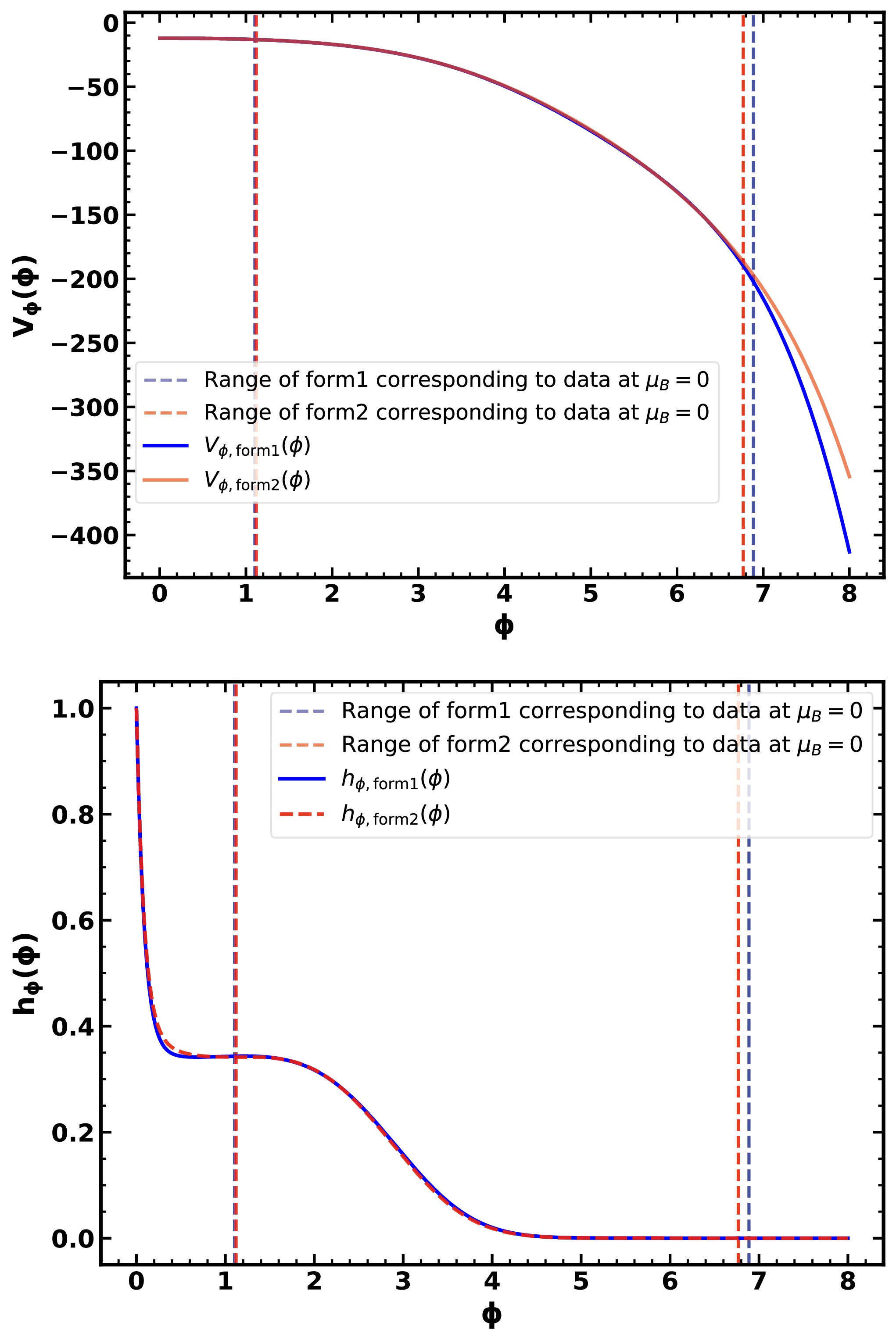
Figure 1. (color online) Robustness check in the probe limit: comparison of the reconstructed model functions
$ V_{\phi,\mathrm{form\,1}}(\phi) $ and$ V_{\phi,\mathrm{form\,2}}(\phi) $ (upper panel), together with$ h_{\phi,\mathrm{form\,1}}(\phi) $ and$ h_{\phi,\mathrm{form\,2}}(\phi) $ (lower panel). The dashed vertical lines indicate the corresponding ϕ ranges covered by the$ \mu_B=0 $ input data, namely approximately$ \phi\simeq 1.104 $ –$ 6.887 $ for form 1 and$ \phi\simeq 1.121 $ –$ 6.768 $ for form 2. Although the two potentials show a visible difference toward the upper end of the fitted interval and beyond, the fitted gauge kinetic functions remain very close, and the resulting thermodynamic observables in the calibrated domain are almost unchanged.$ \begin{aligned}[b] V_{\phi,\mathrm{form\,1},\mathrm{net}}(\phi) =\;&-1.558082\times 10^{-7}\phi^8 +4.058989\times 10^{-6}\phi^7 \\ &-2.014347\times 10^{-5}\phi^6-3.300564\times 10^{-4}\phi^5 \\ &+4.517985\times 10^{-3}\phi^4 -2.073986\times 10^{-2}\phi^3 \\ &+3.797004\times 10^{-2}\phi^2 +6.484887\times 10^{-4}\phi \\ &-1.702365\times 10^{-1}, \end{aligned} $
(70) $ \begin{aligned}[b]h_{\phi,\mathrm{form\,1},\mathrm{net}}(\phi) =7.523421\times 10^{-7}\phi^8 -3.743422\times 10^{-5}\phi^7 \end{aligned} $
$ \begin{aligned}[b] &+7.309245\times 10^{-4}\phi^6 -6.995335\times 10^{-3}\phi^5\\ &+3.262371\times 10^{-2}\phi^4 -6.210014\times 10^{-2}\phi^3\\ &+9.327736\times 10^{-2}\phi^2 -1.261251\times 10^{-1}\phi \\ &+8.025826\times 10^{-2}. \end{aligned} $
(71) In the present probe calibration, the UV input is fixed to
$ \Delta_\phi=3.6 $ and$ \nu=4-\Delta_\phi=0.4 $ , which implies$ m_\phi^2= \Delta_\phi(\Delta_\phi-4)= -1.44 $ . The remaining numerical constants entering the final form-1 parametrization in Eqs. (68)–(69) are$ \begin{aligned}[b]& k_V = -0.1, \quad k_{h_1}^{(1)} = 0.652974, \quad k_{h_2}^{(1)} = -11.292836, \\ &\Lambda = 1130.97\; \mathrm{MeV}, \quad \kappa_5^2 = 10.39. \end{aligned} $
(72) In this probe calibration we take
$ \Delta_\phi=3.6 $ , while in the pure-glue/back-reacted steps below we adopt a different value (e.g.$ \Delta_\phi=3.8 $ ) tailored to that calibration; we keep the same notation to match the corresponding numerical setups.For a limited robustness check, we also consider an alternative probe reconstruction (form 2), obtained from the same dataset and the same two-stage fitting strategy. The common inputs
$ \Delta_\phi=3.6 $ ,$ k_V=-0.1 $ ,$ \Lambda=$ 1130.97 MeV, and$ \kappa_5^2=10.39 $ are kept identical to those of form 1. In this alternative reconstruction, we replace the IR-completion factor$ (1+\phi^2)^{1/4} $ in Eq. (68) by$ (1+\phi^4)^{1/8} $ and adjust the subtraction terms so that the UV expansion remains unchanged. The corresponding reconstructed functions are denoted by$ V_{\phi,\mathrm{form\,2}}(\phi) $ and$ h_{\phi,\mathrm{form\,2}}(\phi) $ , and the alternative probe ansatz is$ \begin{aligned}[b] V_{\phi,\mathrm{form\,2}}(\phi) =\;& -12+\frac{1}{2}m_\phi^2\phi^2 +\phi^4 V_{\phi,\mathrm{form\,2},\mathrm{net}}(\phi) \\ &+k_V(1+\phi^4)^{\frac{1}{8}} \exp \left(\frac{\sqrt{6}}{3}\phi\right) \\ &-\bigg[ k_V+k_V\frac{\sqrt{6}}{3}\phi+\frac{1}{3}k_V\phi^2 \\ & +\frac{\sqrt{6}}{27}k_V\phi^3+\frac{31}{216}k_V\phi^4 \bigg]. \end{aligned} $
(73) $ \begin{aligned}[b] h_{\phi,\mathrm{form\,2}}(\phi) =\;&\,k_{h_1}^{(2)}\exp(k_{h_2}^{(2)}\phi) \\ &+(1-k_{h_1}^{(2)})\exp \left[-\phi\, h_{\phi,\mathrm{form\,2},\mathrm{net}}(\phi)\right]. \end{aligned} $
(74) $ V_{\phi,\mathrm{form\,2},\mathrm{net}}(\phi) =\frac{ -1.950922\times 10^{-1} +1.445155\times 10^{-1}\phi -6.301410\times 10^{-2}\phi^2 +9.142151\times 10^{-3}\phi^3 -4.844424\times 10^{-4}\phi^4 }{ 1.0 -4.783528\times 10^{-1}\phi +2.448851\times 10^{-1}\phi^2 -3.530235\times 10^{-2}\phi^3 +3.506043\times 10^{-3}\phi^4 }, $
(75) $ \begin{aligned}[b] h_{\phi,\mathrm{form\,2},\mathrm{net}}(\phi) =\;&-1.890023\times 10^{-6}\phi^8 +4.620669\times 10^{-5}\phi^7 \\ &-3.758841\times 10^{-4}\phi^6 +1.032000\times 10^{-3}\phi^5 \\ &-1.816022\times 10^{-3}\phi^4 +1.945701\times 10^{-2}\phi^3 \\ &+2.840613\times 10^{-2}\phi^2-2.342798\times 10^{-1}\phi \\ &+3.127162\times 10^{-1}, \end{aligned} $
(76) $ \begin{aligned}[b] k_{h_1}^{(2)} = 0.612463, \qquad k_{h_2}^{(2)} = -11.600600. \end{aligned} $
(77) Here
$ V_{\phi,\mathrm{form\,2},\mathrm{net}}(\phi) $ and$ h_{\phi,\mathrm{form\,2},\mathrm{net}}(\phi) $ denote the retrained flexible components in the alternative calibration. The free part still starts at order$ \phi^4 $ , so the UV mass term remains fixed by$ \Delta_\phi $ and is not mixed with the flexible interior part. The new factor$ (1+\phi^4)^{1/8} $ preserves the same leading IR behavior$ \phi^{1/2}\exp(\sqrt{6}\phi/3) $ , while modifying the interpolation pattern at intermediate ϕ. As in form 1, the flexible part reconstructed by the neural ODE is data-driven, and its explicit polynomial or rational expression is used only as a convenient parametrization in the data-constrained range. With the same UV input$ \Delta_\phi=3.6 $ ,$ \nu=0.4 $ ,$ m_\phi^2=-1.44 $ , and the same overall constants$ \Lambda=1130.97\; \mathrm{MeV} $ and$ \kappa_5^2=10.39 $ , we refit the model and obtain the form-2 probe EoS. The resulting curves of$ s/T^3 $ ,$ p/T^4 $ ,$ \epsilon/T^4 $ ,$ I/T^4 $ , and$ n_B/T^3 $ in the calibrated domain remain almost unchanged, indicating that the probe-limit results are stable under this nontrivial change of the probe ansatz. This limited check concerns these calibrated thermodynamic observables only, and is not meant to constrain extrapolative quantities such as the CEP position.The training is performed in two stages. First, we fix
$ \mu=0 $ and optimize$ V_{\phi}(\phi) $ by matching$ s/T^3 $ . Second, we freeze the trained$ V_{\phi}(\phi) $ and optimize$ h_\phi(\phi) $ by matching both$ s/T^3 $ and$ n_B/T^3 $ at finite μ. For a data sample at$ (T_i,\mu_i) $ with uncertainty$ e_i $ , we define the loss functions as$ L_{s/T^3} =\frac{1}{N}\sum\limits_i \left[ \frac{\left(s/T^3\right)_{m_i}-\left(s/T^3\right)_{d_i}}{\left(s/T^3\right)_{e_i}} \right]^2, $
(78) $ \begin{aligned}[b] L_{n_B/T^3} =\;&\frac{1}{N}\sum\limits_i \left[ \Big(\ln \left(n_B/T^3\right)_{m_i}-\ln \left(n_B/T^3\right)_{d_i}\Big) \frac{\left(n_B/T^3\right)_{d_i}}{\left(n_B/T^3\right)_{e_i}} \right]^2, \end{aligned} $
(79) where the subscripts
$ m_i $ ,$ d_i $ , and$ e_i $ denote the model prediction, the reference-data value, and the data uncertainty, respectively. The logarithmic form in Eq. (79) balances the wide dynamic range of$ n_B/T^3 $ . We solve the equations of motion (EoMs) using a differentiable ODE solver, and optimize the neural network parameters via gradient-based optimization methods. The corresponding neural-ODE calibration workflow is shown schematically in Fig. 2.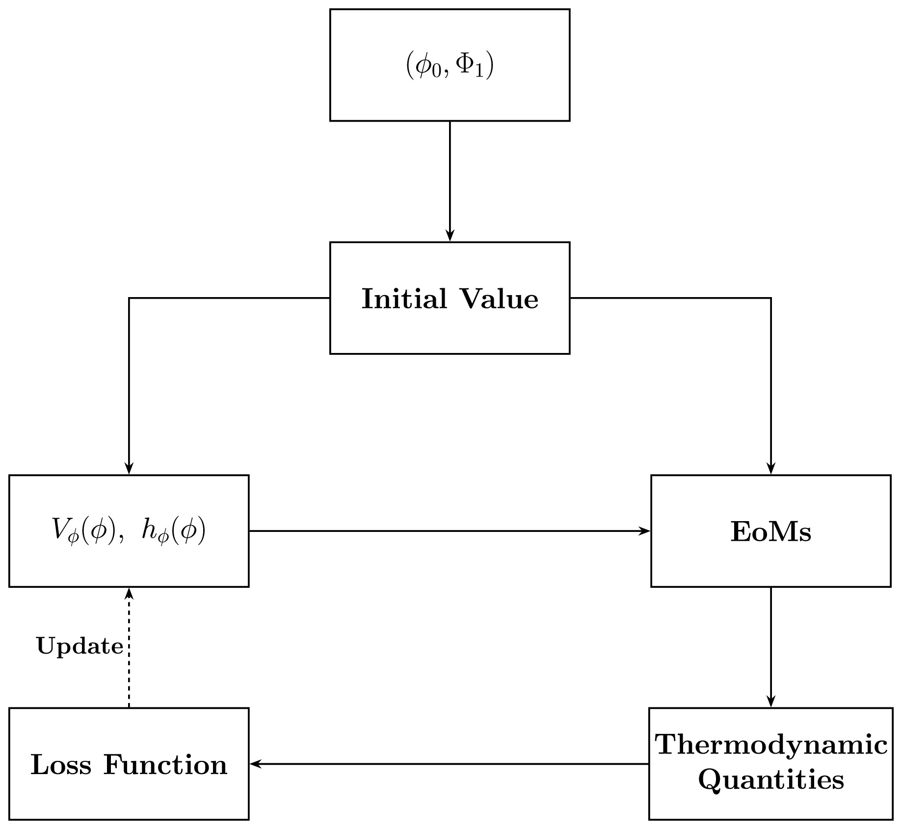
Figure 2. Schematic illustration of the neural-ODE calibration workflow. For a given set of model-function parameters, the EMD equations are solved to obtain thermodynamic observables, which are compared with the reference table to construct the loss. The parameters are then updated through gradient-based optimization.
-
In this part, we calibrate the EMD model to the lattice EoS using neural ODE framework [29, 30]. The EMD equations are treated as a differentiable ODE system, and the model functions
$ V_{\phi}(\phi) $ and$ h_{\phi}(\phi) $ are learned from data under UV/IR constraints. The parameters are optimized by minimizing the mismatch between the holographic predictions and the lattice targets.Once
$ V_{\phi}(\phi) $ and$ h_{\phi}(\phi) $ are determined, we keep them fixed and use the same five-dimensional action for all black-hole solutions at different$ (T,\mu_B) $ . This keeps the thermodynamic state dependence in the solutions rather than in temperature-dependent effective potentials, and makes the subsequent back-reaction study a direct probe of the limitations of the coupled ansatz. If the model functions were also allowed to vary with the thermodynamic state, it would become harder to distinguish the fixed bulk action from the state-dependent black-hole solutions, and the subsequent back-reaction analysis would be less transparent.In this probe calibration, we use as a reference a recently published thermodynamic table for
$ (2+1) $ -flavor QCD at finite temperature and finite baryon chemical potential, with$ \mu_Q=\mu_S=0 $ and$ T=35.0 $ –$ 490.0\; \mathrm{MeV} $ [49]. This table is released through a public interpolation/fitting framework that combines lattice-QCD constraints with a hadron-resonance-gas (HRG) description [50], and provides a broad and smooth domain that is convenient for a stable inverse reconstruction of the model functions. Our conventions for the EMD background and thermodynamic extraction follow standard choices in the recent holographic EMD literature; see, e.g., Ref. [15]. In our training set, we include the dimensionless ratio$ s/T^3 $ (and thus also$ p/T^4 $ ,$ \epsilon/T^4 $ , and$ I/T^4\equiv(\epsilon-3p)/T^4 $ derived from thermodynamic identities) at$ \mu=0 $ , together with$ s/T^3 $ and$ n_B/T^3 $ at finite μ.To reduce degeneracies in the inverse fit, we build the model functions by combining hard UV/IR constraints with a flexible data-driven component. Specifically, we impose the UV behavior
$ V_{\phi}(\phi)=-12+\frac{1}{2}m_\phi^2\phi^2+\mathcal{O}(\phi^4) $ and$ h_\phi(\phi)=1+\mathcal{O}(\phi) $ at$ \phi\to 0 $ . The UV mass term is fixed by the scaling dimension$ \Delta_\phi $ through the AdS/CFT relation in Eq. (11); see also the discussion in Sec. II. According to Refs. [51, 52], if one requires confinement and the absence of bad singularities, the IR asymptotics of the dilaton potential should satisfy$ \begin{aligned}[b] &L^2V_{\phi}(\phi\to+\infty) =c_{V}\,\mathrm{e}^{c_{\phi,1}\phi+\cdots} \left(\phi^{c_{\phi,2}}+\cdots\right), \\ &\left\{ \begin{aligned} &\frac{\sqrt{6}}{3}<c_{\phi,1}<\frac{2\sqrt{3}}{3}, \quad c_{\phi,2}\ \text{real},\\ &c_{\phi,1}=\frac{\sqrt{6}}{3}, \quad c_{\phi,2}\geqslant 0, \end{aligned} \right. \end{aligned} $
(66) with
$ c_V $ a constant. When$ c_{\phi,1}=\sqrt{6}/3 $ and$ c_{\phi,2}>0 $ , the asymptotic glueball spectrum behaves as$ \begin{array}{l} m_n\sim n^{c_{\phi,2}} \qquad \text{when} \quad n\to+\infty, \end{array} $
(67) and the choice
$ c_{\phi,2}=1/2 $ gives asymptotically linear Regge behavior. In the IR we therefore include a term consistent with this class and set$ \Delta_\phi=3.6 $ (thus$ \nu=4-\Delta_\phi=0.4 $ and$ m_\phi^2=\Delta_\phi(\Delta_\phi-4) $ ) together with a fixed IR coefficient$ k_V=-0.1 $ . The remaining parts of$ V_{\phi}(\phi) $ and$ h_\phi(\phi) $ are then learned from data in the neural-ODE optimization. In practice, the flexible components are represented by fully connected neural networks with a simple$ 1 $ –$ 24 $ –$ 24 $ –$ 1 $ architecture and SiLU activation.For later use, we provide an explicit functional parametrization for the reconstructed model functions in the original probe calibration. To match the legends used in the figures below, we denote this original reconstruction by form 1, with model functions
$ V_{\phi,\mathrm{form\,1}}(\phi) $ and$ h_{\phi,\mathrm{form\,1}}(\phi) $ . In our convention, the Einstein-frame gluon potential and the gauge kinetic function are taken as$ \begin{aligned}[b] V_{\phi,\mathrm{form\,1}}(\phi) =\;& -12+\frac{1}{2}m_\phi^2\phi^2 +\phi^4 V_{\phi,\mathrm{form\,1},\mathrm{net}}(\phi) \\ &+k_V(1+\phi^2)^{\frac{1}{4}} \exp \left(\frac{\sqrt{6}}{3}\phi\right) \\ &-\bigg[ k_V+k_V\frac{\sqrt{6}}{3}\phi+\frac{7}{12}k_V\phi^2 \\ & +\frac{13}{36}k_V\frac{\sqrt{6}}{3}\phi^3+\frac{5}{288}k_V\phi^4 \bigg], \end{aligned} $
(68) and
$ \begin{aligned}[b] h_{\phi,\mathrm{form\,1}}(\phi) =\;&\,k_{h_1}^{(1)}\exp(k_{h_2}^{(1)}\phi) \\ &+(1-k_{h_1}^{(1)})\exp \left[-\phi\, h_{\phi,\mathrm{form\,1},\mathrm{net}}(\phi)\right], \end{aligned} $
(69) where
$ V_{\phi,\mathrm{form\,1},\mathrm{net}}(\phi) $ and$ h_{\phi,\mathrm{form\,1},\mathrm{net}}(\phi) $ denote the flexible components represented by neural networks. The subtraction terms in Eq. (68) ensure that the UV expansion matches$ V_{\phi}(\phi)=-12+\dfrac{1}{2}m_\phi^2\phi^2+\mathcal{O}(\phi^4) $ while keeping the desired IR asymptotics. The free function is multiplied by$ \phi^4 $ , rather than by$ \phi^2 $ , so that the UV mass term remains fixed by the relation$ m_{\phi}^{2}L^{2}=\Delta_{\phi}(\Delta_{\phi}-4) $ and is not contaminated by the flexible interior parametrization. The explicit polynomial fit for$ V_{\phi,\mathrm{form\,1},\mathrm{net}}(\phi) $ given below is used only as a convenient representation of the trained function in the data-constrained range, and is not itself the object of the robustness check discussed later.For future reference, we fit the trained form-1 network outputs using simple polynomials (valid in the data-constrained range of ϕ shown in Fig. 1):
Figure 1. (color online) Robustness check in the probe limit: comparison of the reconstructed model functions
$ V_{\phi,\mathrm{form\,1}}(\phi) $ and$ V_{\phi,\mathrm{form\,2}}(\phi) $ (upper panel), together with$ h_{\phi,\mathrm{form\,1}}(\phi) $ and$ h_{\phi,\mathrm{form\,2}}(\phi) $ (lower panel). The dashed vertical lines indicate the corresponding ϕ ranges covered by the$ \mu_B=0 $ input data, namely approximately$ \phi\simeq 1.104 $ –$ 6.887 $ for form 1 and$ \phi\simeq 1.121 $ –$ 6.768 $ for form 2. Although the two potentials show a visible difference toward the upper end of the fitted interval and beyond, the fitted gauge kinetic functions remain very close, and the resulting thermodynamic observables in the calibrated domain are almost unchanged.$ \begin{aligned}[b] V_{\phi,\mathrm{form\,1},\mathrm{net}}(\phi) =\;&-1.558082\times 10^{-7}\phi^8 +4.058989\times 10^{-6}\phi^7 \\ &-2.014347\times 10^{-5}\phi^6-3.300564\times 10^{-4}\phi^5 \\ &+4.517985\times 10^{-3}\phi^4 -2.073986\times 10^{-2}\phi^3 \\ &+3.797004\times 10^{-2}\phi^2 +6.484887\times 10^{-4}\phi \\ &-1.702365\times 10^{-1}, \end{aligned} $
(70) $ \begin{aligned}[b]h_{\phi,\mathrm{form\,1},\mathrm{net}}(\phi) =7.523421\times 10^{-7}\phi^8 -3.743422\times 10^{-5}\phi^7 \end{aligned} $
$ \begin{aligned}[b] &+7.309245\times 10^{-4}\phi^6 -6.995335\times 10^{-3}\phi^5\\ &+3.262371\times 10^{-2}\phi^4 -6.210014\times 10^{-2}\phi^3\\ &+9.327736\times 10^{-2}\phi^2 -1.261251\times 10^{-1}\phi \\ &+8.025826\times 10^{-2}. \end{aligned} $
(71) In the present probe calibration, the UV input is fixed to
$ \Delta_\phi=3.6 $ and$ \nu=4-\Delta_\phi=0.4 $ , which implies$ m_\phi^2=\Delta_\phi(\Delta_\phi-4)=-1.44 $ . The remaining numerical constants entering the final form-1 parametrization in Eqs. (68)–(69) are$ \begin{aligned}[b]& k_V = -0.1, \quad k_{h_1}^{(1)} = 0.652974, \quad k_{h_2}^{(1)} = -11.292836, \\ &\Lambda = 1130.97\; \mathrm{MeV}, \quad \kappa_5^2 = 10.39. \end{aligned} $
(72) In this probe calibration we take
$ \Delta_\phi=3.6 $ , while in the pure-glue/back-reacted steps below we adopt a different value (e.g.$ \Delta_\phi=3.8 $ ) tailored to that calibration; we keep the same notation to match the corresponding numerical setups.For a limited robustness check, we also consider an alternative probe reconstruction (form 2), obtained from the same dataset and the same two-stage fitting strategy. The common inputs
$ \Delta_\phi=3.6 $ ,$ k_V=-0.1 $ ,$ \Lambda=1130.97\; \mathrm{MeV} $ , and$ \kappa_5^2=10.39 $ are kept identical to those of form 1. In this alternative reconstruction, we replace the IR-completion factor$ (1+\phi^2)^{1/4} $ in Eq. (68) by$ (1+\phi^4)^{1/8} $ and adjust the subtraction terms so that the UV expansion remains unchanged. The corresponding reconstructed functions are denoted by$ V_{\phi,\mathrm{form\,2}}(\phi) $ and$ h_{\phi,\mathrm{form\,2}}(\phi) $ , and the alternative probe ansatz is$ \begin{aligned}[b] V_{\phi,\mathrm{form\,2}}(\phi) =\;& -12+\frac{1}{2}m_\phi^2\phi^2 +\phi^4 V_{\phi,\mathrm{form\,2},\mathrm{net}}(\phi) \\ &+k_V(1+\phi^4)^{\frac{1}{8}} \exp \left(\frac{\sqrt{6}}{3}\phi\right) \\ &-\bigg[ k_V+k_V\frac{\sqrt{6}}{3}\phi+\frac{1}{3}k_V\phi^2 \\ & +\frac{\sqrt{6}}{27}k_V\phi^3+\frac{31}{216}k_V\phi^4 \bigg]. \end{aligned} $
(73) $ \begin{aligned}[b] h_{\phi,\mathrm{form\,2}}(\phi) =\;&\,k_{h_1}^{(2)}\exp(k_{h_2}^{(2)}\phi) \\ &+(1-k_{h_1}^{(2)})\exp \left[-\phi\, h_{\phi,\mathrm{form\,2},\mathrm{net}}(\phi)\right]. \end{aligned} $
(74) $ V_{\phi,\mathrm{form\,2},\mathrm{net}}(\phi) =\frac{ -1.950922\times 10^{-1} +1.445155\times 10^{-1}\phi -6.301410\times 10^{-2}\phi^2 +9.142151\times 10^{-3}\phi^3 -4.844424\times 10^{-4}\phi^4 }{ 1.0 -4.783528\times 10^{-1}\phi +2.448851\times 10^{-1}\phi^2 -3.530235\times 10^{-2}\phi^3 +3.506043\times 10^{-3}\phi^4 }, $
(75) $ \begin{aligned}[b] h_{\phi,\mathrm{form\,2},\mathrm{net}}(\phi) =\;&-1.890023\times 10^{-6}\phi^8 +4.620669\times 10^{-5}\phi^7 \\ &-3.758841\times 10^{-4}\phi^6 +1.032000\times 10^{-3}\phi^5 \\ &-1.816022\times 10^{-3}\phi^4 +1.945701\times 10^{-2}\phi^3 \\ &+2.840613\times 10^{-2}\phi^2-2.342798\times 10^{-1}\phi \\ &+3.127162\times 10^{-1}, \end{aligned} $
(76) $ \begin{aligned}[b] k_{h_1}^{(2)} = 0.612463, \qquad k_{h_2}^{(2)} = -11.600600. \end{aligned} $
(77) Here
$ V_{\phi,\mathrm{form\,2},\mathrm{net}}(\phi) $ and$ h_{\phi,\mathrm{form\,2},\mathrm{net}}(\phi) $ denote the retrained flexible components in the alternative calibration. The free part still starts at order$ \phi^4 $ , so the UV mass term remains fixed by$ \Delta_\phi $ and is not mixed with the flexible interior part. The new factor$ (1+\phi^4)^{1/8} $ preserves the same leading IR behavior$ \phi^{1/2}\exp(\sqrt{6}\phi/3) $ , while modifying the interpolation pattern at intermediate ϕ. As in form 1, the flexible part reconstructed by the neural ODE is data-driven, and its explicit polynomial or rational expression is used only as a convenient parametrization in the data-constrained range. With the same UV input$ \Delta_\phi=3.6 $ ,$ \nu=0.4 $ ,$ m_\phi^2=-1.44 $ , and the same overall constants$ \Lambda=1130.97\; \mathrm{MeV} $ and$ \kappa_5^2=10.39 $ , we refit the model and obtain the form-2 probe EoS shown in Figs. 5 and 6. The resulting curves of$ s/T^3 $ ,$ p/T^4 $ ,$ \epsilon/T^4 $ ,$ I/T^4 $ , and$ n_B/T^3 $ in the calibrated domain remain almost unchanged, indicating that the probe-limit results are stable under this nontrivial change of the probe ansatz. This limited check concerns these calibrated thermodynamic observables only, and is not meant to constrain extrapolative quantities such as the CEP position.
Figure 5. (color online) Probe approximation,
$ (2+1) $ flavors at$ \mu=0 $ , form 2: a comparison between the holographic EMD results (solid lines) and the reference thermodynamic table [49] (scatter points). Upper left panel:$ s/T^3 $ ; upper right panel:$ p/T^4 $ ; lower left panel:$ \epsilon/T^4 $ ; lower right panel:$ I/T^4=(\epsilon-3p)/T^4 $ . The reference points for$ I/T^4 $ are constructed from the combination$ \epsilon-3p $ and thus do not represent an independently tabulated observable. The horizontal axis is T in units of MeV.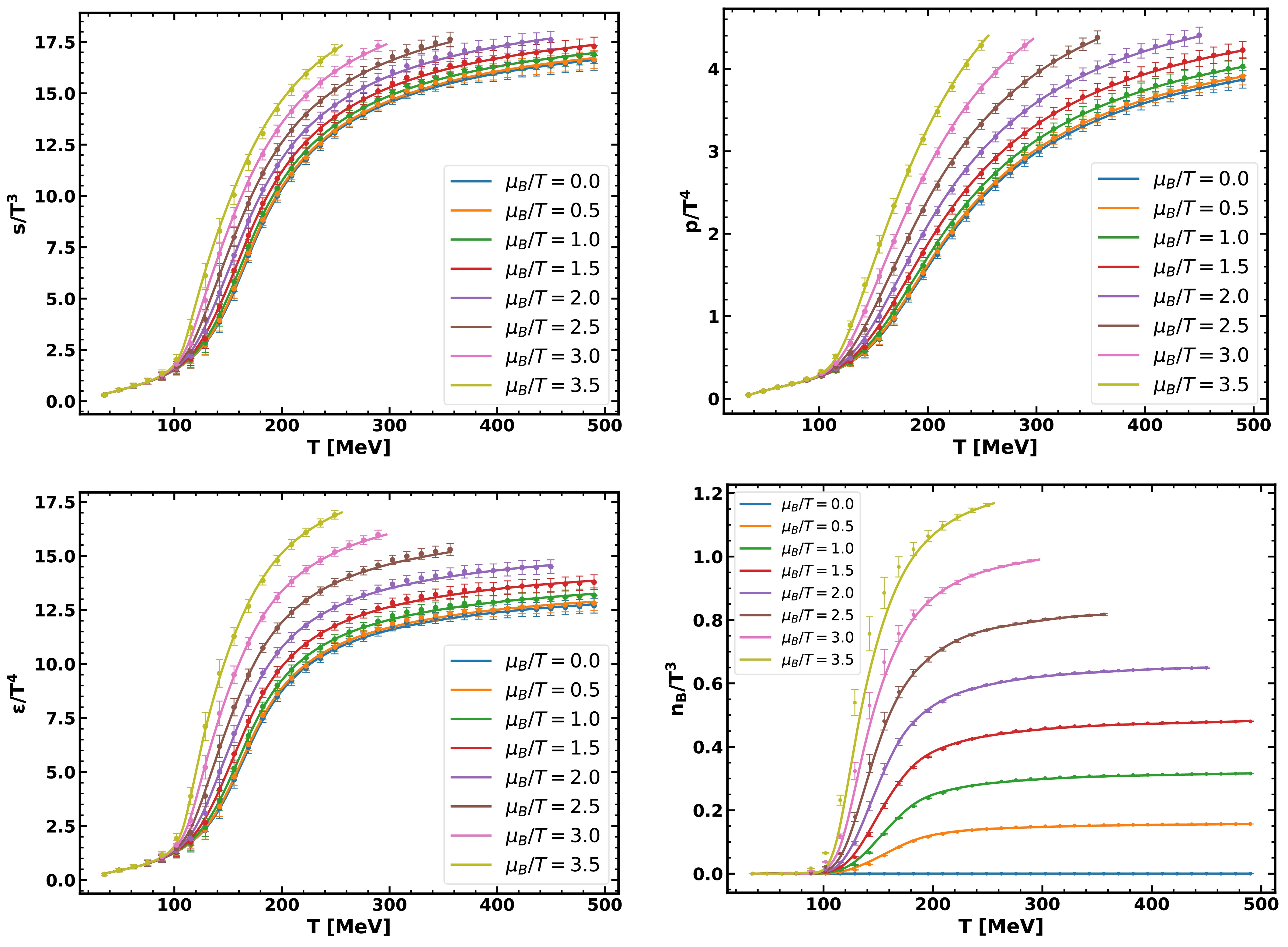
Figure 6. (color online) Probe approximation,
$ (2+1) $ flavors in fixed$ \mu/T $ slices (temperature window$ T=35 $ –$ 490\; \mathrm{MeV} $ ), form 2: comparisons between the holographic EMD results (solid lines) and the reference thermodynamic table [49] (scatter points). Upper left panel:$ s/T^3 $ ; upper right panel:$ p/T^4 $ ; lower left panel:$ \epsilon/T^4 $ ; lower right panel:$ n_B/T^3 $ .The training is performed in two stages. First, we fix
$ \mu=0 $ and optimize$ V_{\phi}(\phi) $ by matching$ s/T^3 $ . Second, we freeze the trained$ V_{\phi}(\phi) $ and optimize$ h_\phi(\phi) $ by matching both$ s/T^3 $ and$ n_B/T^3 $ at finite μ. For a data sample at$ (T_i,\mu_i) $ with uncertainty$ e_i $ , we define the loss functions as$ L_{s/T^3} =\frac{1}{N}\sum\limits_i \left[ \frac{\left(s/T^3\right)_{m_i}-\left(s/T^3\right)_{d_i}}{\left(s/T^3\right)_{e_i}} \right]^2, $
(78) $ \begin{aligned}[b] L_{n_B/T^3} =\;&\frac{1}{N}\sum\limits_i \left[ \Big(\ln \left(n_B/T^3\right)_{m_i}-\ln \left(n_B/T^3\right)_{d_i}\Big) \right. \\ &\left. \times \frac{\left(n_B/T^3\right)_{d_i}}{\left(n_B/T^3\right)_{e_i}} \right]^2, \end{aligned} $
(79) where the subscripts
$ m_i $ ,$ d_i $ , and$ e_i $ denote the model prediction, the reference-data value, and the data uncertainty, respectively. The logarithmic form in Eq. (79) balances the wide dynamic range of$ n_B/T^3 $ . We solve the equations of motion (EoMs) using a differentiable ODE solver, and optimize the neural network parameters via gradient-based optimization methods. -
After training, we obtain an excellent agreement with the reference thermodynamic table for
$ (2+1) $ -flavor QCD in a wide range of temperature and chemical potential. For the original probe reconstruction (form 1), representative comparisons at$ \mu=0 $ are shown in Fig. 3, while the comparisons in fixed$ \mu/T $ slices in the temperature window$ T=35 $ –$ 490\; \mathrm{MeV} $ are shown in Fig. 4. The corresponding form-2 results are shown in Figs. 5 and 6.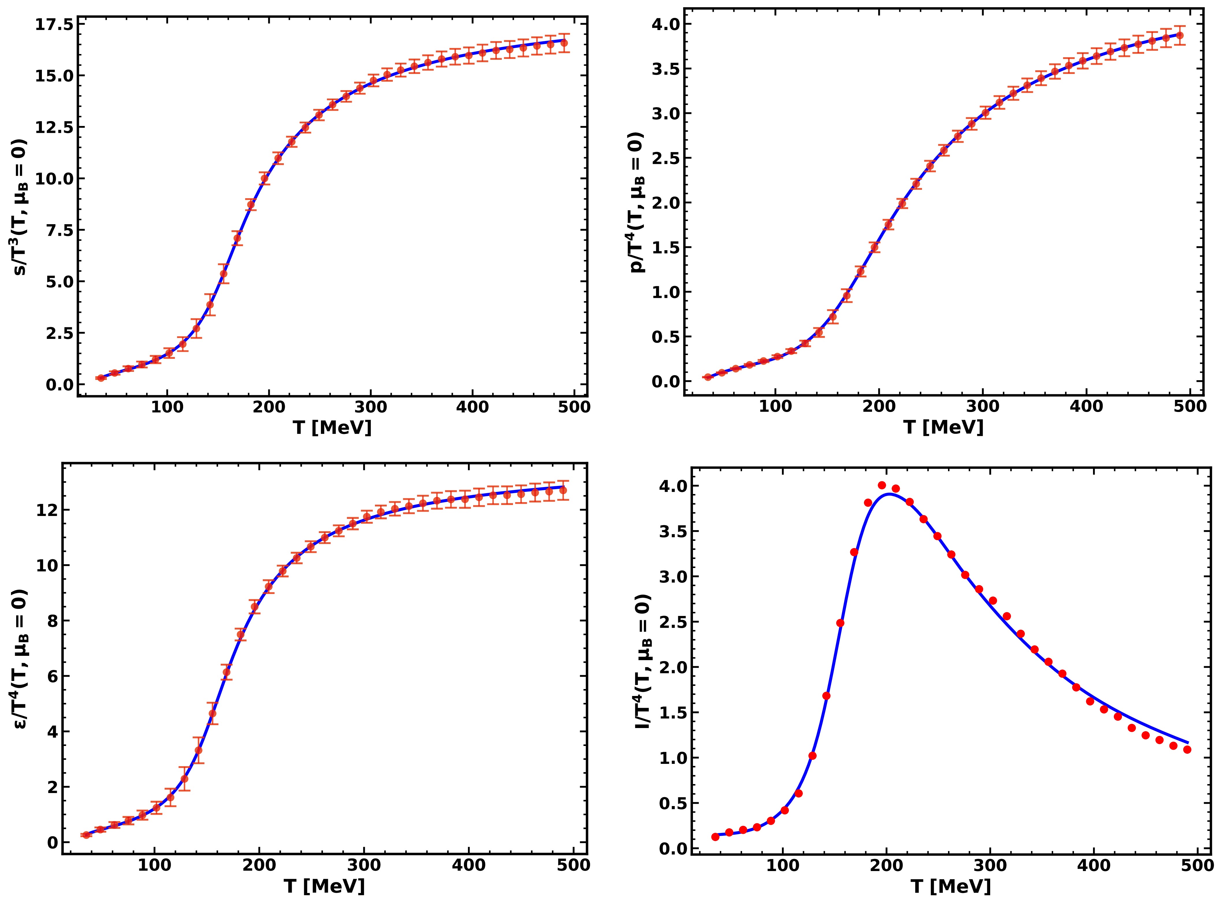
Figure 3. (color online) Probe approximation,
$ (2+1) $ flavors at$ \mu=0 $ , form 1: comparison between the holographic EMD results (solid lines) and the reference thermodynamic table [49] (scatter points). Upper left panel:$ s/T^3 $ ; upper right panel:$ p/T^4 $ ; lower left panel:$ \epsilon/T^4 $ ; lower right panel:$ I/T^4=(\epsilon-3p)/T^4 $ . The reference points for$ I/T^4 $ are constructed from the combination$ \epsilon-3p $ , and thus do not represent an independently tabulated observable. The horizontal axis is T in units of MeV.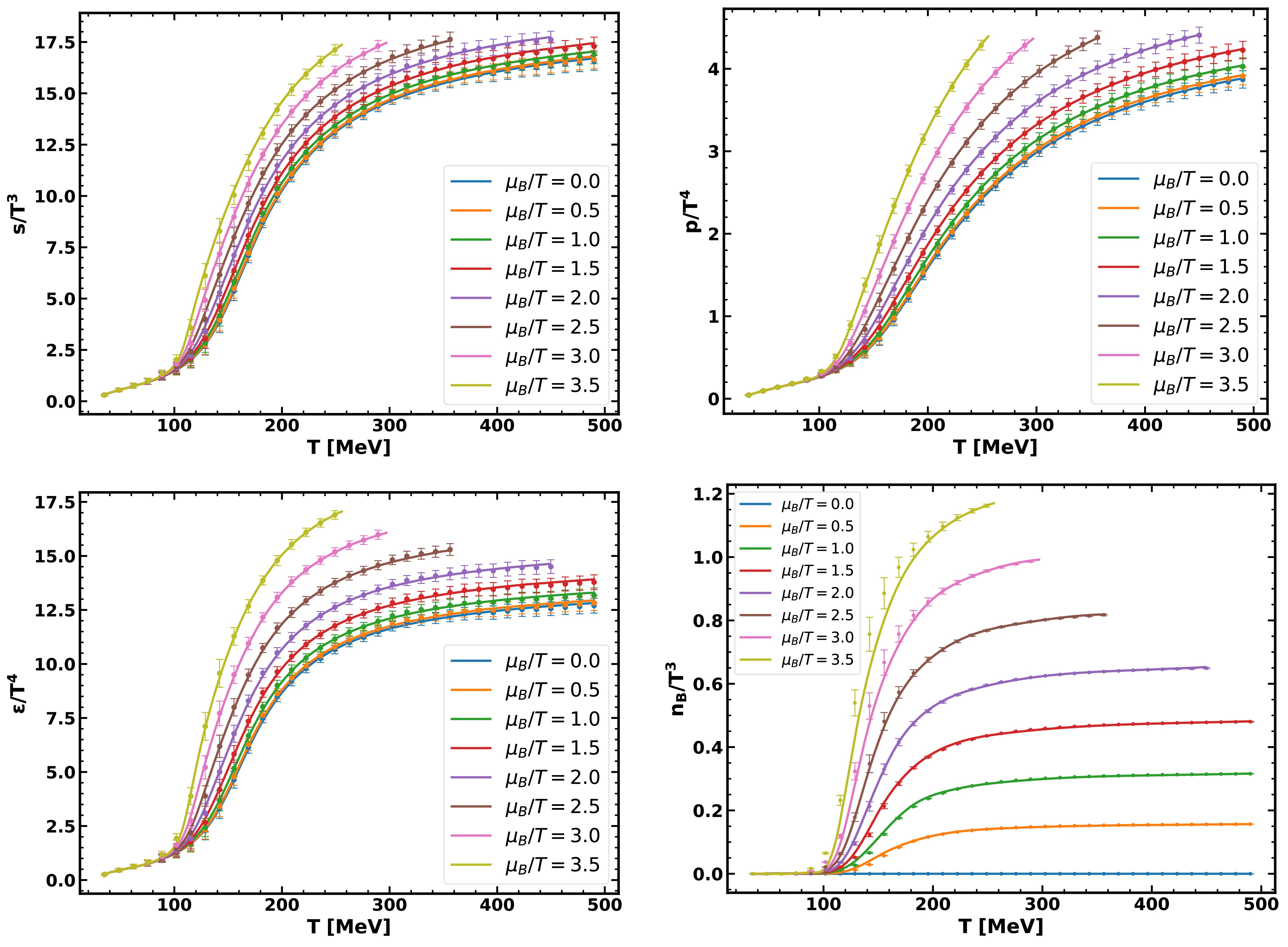
Figure 4. (color online) Probe approximation,
$ (2+1) $ flavors in fixed$ \mu/T $ slices (temperature window$ T=35 $ –$ 490\; \mathrm{MeV} $ ), form 1: comparisons between the holographic EMD results (solid lines) and the reference thermodynamic table [49] (scatter points). Upper left panel:$ s/T^3 $ ; upper right panel:$ p/T^4 $ ; lower left panel:$ \epsilon/T^4 $ ; lower right panel:$ n_B/T^3 $ .
Figure 5. (color online) Probe approximation,
$ (2+1) $ flavors at$ \mu=0 $ , form 2: a comparison between the holographic EMD results (solid lines) and the reference thermodynamic table [49] (scatter points). Upper left panel:$ s/T^3 $ ; upper right panel:$ p/T^4 $ ; lower left panel:$ \epsilon/T^4 $ ; lower right panel:$ I/T^4=(\epsilon-3p)/T^4 $ . The reference points for$ I/T^4 $ are constructed from the combination$ \epsilon-3p $ and thus do not represent an independently tabulated observable. The horizontal axis is T in units of MeV.
Figure 6. (color online) Probe approximation,
$ (2+1) $ flavors in fixed$ \mu/T $ slices (temperature window$ T=35 $ –$ 490\; \mathrm{MeV} $ ), form 2: comparisons between the holographic EMD results (solid lines) and the reference thermodynamic table [49] (scatter points). Upper left panel:$ s/T^3 $ ; upper right panel:$ p/T^4 $ ; lower left panel:$ \epsilon/T^4 $ ; lower right panel:$ n_B/T^3 $ .As an additional application of the reconstructed probe-approximation model, one may explore the thermodynamics at finite μ and infer the possible location of the critical endpoint (CEP). Following the standard procedure, we inspect the behavior of
$ T(s,\mu_B) $ and identify the CEP from the extremum of$ \mathrm{d}T/\mathrm{d}s $ along fixed-$ \mu_B $ curves. An illustration of this determination for form 1 is shown in Fig. 7. For completeness, the corresponding determination for form 2 is shown in Fig. 8. From these plots, the CEP of the form-1 reconstructed probe model is estimated in the range$ T^{\mathrm{CEP}}\simeq 89.35 $ –$ 89.50\; \mathrm{MeV} $ and$ \mu_B^{\mathrm{CEP}}\simeq 630 $ –$ 631\; \mathrm{MeV} $ , while that of the form-2 reconstructed probe model is estimated in the range$ T^{\mathrm{CEP}}\simeq 89.20 $ –$ 89.35\; \mathrm{MeV} $ and$ \mu_B^{\mathrm{CEP}}\simeq 645 $ –$ 646\; \mathrm{MeV} $ .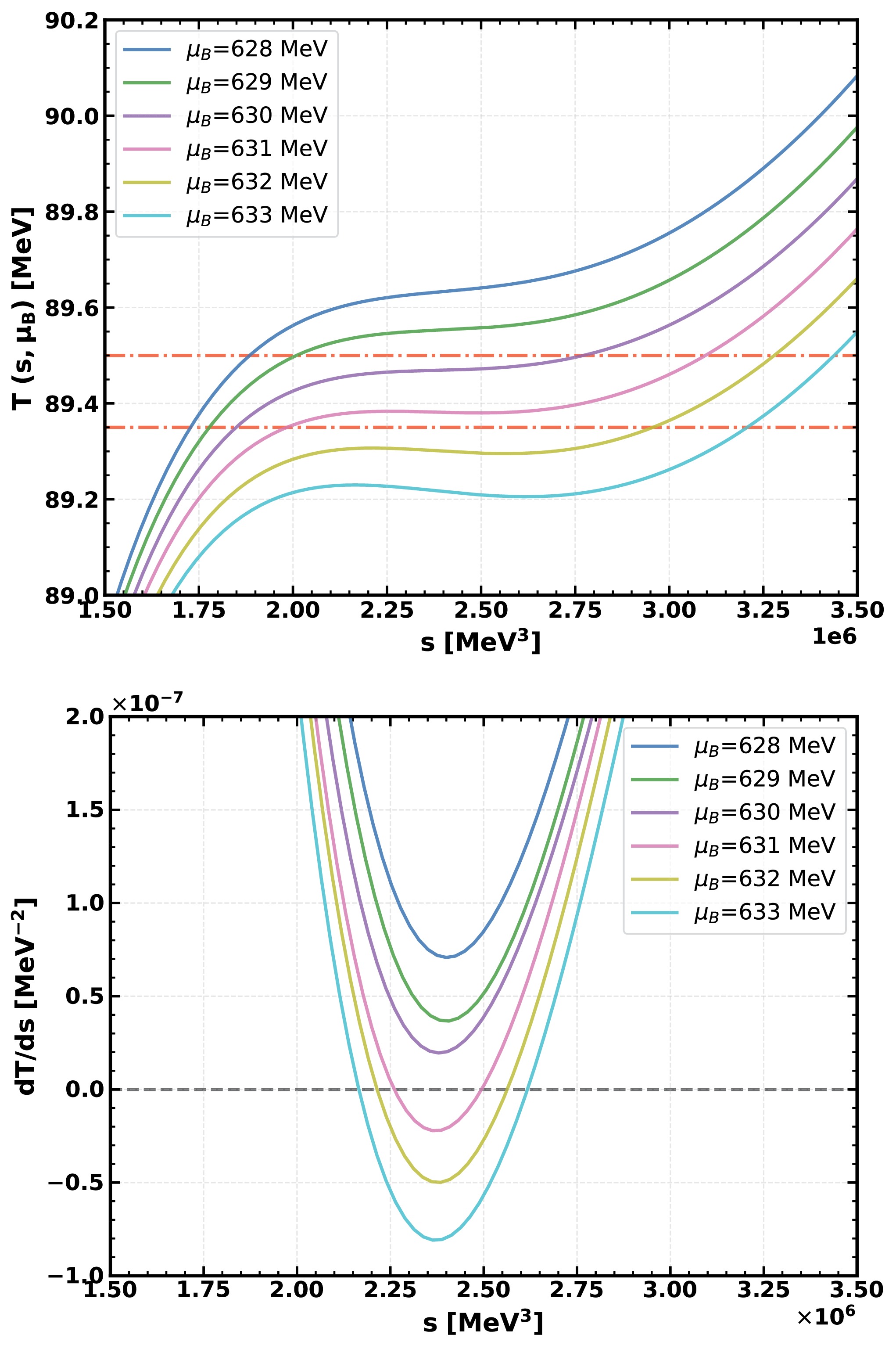
Figure 7. (color online) Determination of the QCD critical endpoint (CEP) in the probe-approximation model, form 1. Upper panel:
$ T(s,\mu_B) $ curves for several nearby values of$ \mu_B $ , used to bracket the CEP in a narrow range; the dash-dotted horizontal lines indicate the corresponding estimated temperature interval. Lower panel:$ \mathrm{d}T/\mathrm{d}s $ as a function of s for the same set of$ \mu_B $ values, showing how the extremum changes sign across the CEP region.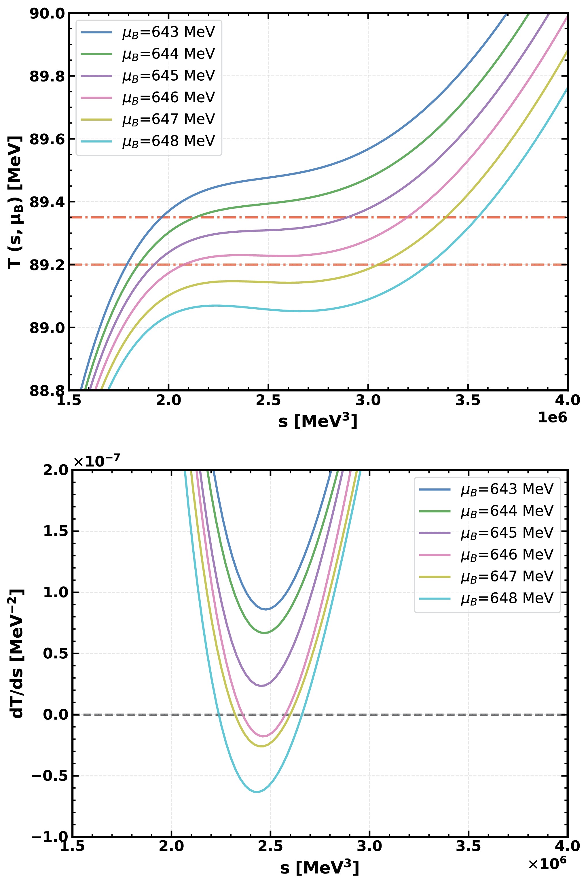
Figure 8. (color online) Determination of the QCD critical endpoint (CEP) in the probe-approximation model, form 2. Upper panel:
$ T(s,\mu_B) $ curves for several nearby values of$ \mu_B $ , used to bracket the CEP in a narrow range; the dash-dotted horizontal lines indicate the corresponding estimated temperature interval. Lower panel:$ \mathrm{d}T/\mathrm{d}s $ as a function of s for the same set of$ \mu_B $ values, showing how the extremum changes sign across the CEP region. -
After training, we obtain an excellent agreement with the reference thermodynamic table for
$ (2+1) $ -flavor QCD in a wide range of temperature and chemical potential. For the original probe reconstruction (form 1), representative comparisons at$ \mu=0 $ are shown in Fig. 3, while the comparisons in fixed$ \mu/T $ slices in the temperature window$ T=35 $ –$ 490\; \mathrm{MeV} $ are shown in Fig. 4. The corresponding form-2 results are shown in Figs. 5 and 6.
Figure 3. (color online) Probe approximation,
$ (2+1) $ flavors at$ \mu=0 $ , form 1: comparison between the holographic EMD results (solid lines) and the reference thermodynamic table [49] (scatter points). Upper left panel:$ s/T^3 $ ; upper right panel:$ p/T^4 $ ; lower left panel:$ \epsilon/T^4 $ ; lower right panel:$ I/T^4=(\epsilon-3p)/T^4 $ . The reference points for$ I/T^4 $ are constructed from the combination$ \epsilon-3p $ , and thus do not represent an independently tabulated observable. The horizontal axis is T in units of MeV.
Figure 4. (color online) Probe approximation,
$ (2+1) $ flavors in fixed$ \mu/T $ slices (temperature window$ T=35 $ –$ 490\; \mathrm{MeV} $ ), form 1: comparisons between the holographic EMD results (solid lines) and the reference thermodynamic table [49] (scatter points). Upper left panel:$ s/T^3 $ ; upper right panel:$ p/T^4 $ ; lower left panel:$ \epsilon/T^4 $ ; lower right panel:$ n_B/T^3 $ .As an additional application of the reconstructed probe-approximation model, one may explore the thermodynamics at finite μ and infer the possible location of the critical endpoint (CEP). Following the standard procedure, we inspect the behavior of
$ T(s,\mu_B) $ and identify the CEP from the extremum of$ \mathrm{d}T/\mathrm{d}s $ along fixed-$ \mu_B $ curves. An illustration of this determination for form 1 is shown in Fig. 7. For completeness, the corresponding determination for form 2 is shown in Fig. 8. From these plots, the CEP of the form-1 reconstructed probe model is estimated in the range$ T^{\mathrm{CEP}}\simeq 89.35 $ –$ 89.50\; \mathrm{MeV} $ and$ \mu_B^{\mathrm{CEP}}\simeq 630 $ –$ 631\; \mathrm{MeV} $ , while that of the form-2 reconstructed probe model is estimated in the range$ T^{\mathrm{CEP}}\simeq 89.20 $ –$ 89.35\; \mathrm{MeV} $ and$ \mu_B^{\mathrm{CEP}}\simeq 645 $ –$ 646\; \mathrm{MeV} $ .
Figure 7. (color online) Determination of the QCD critical endpoint (CEP) in the probe-approximation model, form 1. Upper panel:
$ T(s,\mu_B) $ curves for several nearby values of$ \mu_B $ , used to bracket the CEP in a narrow range; the dash-dotted horizontal lines indicate the corresponding estimated temperature interval. Lower panel:$ \mathrm{d}T/\mathrm{d}s $ as a function of s for the same set of$ \mu_B $ values, showing how the extremum changes sign across the CEP region.
Figure 8. (color online) Determination of the QCD critical endpoint (CEP) in the probe-approximation model, form 2. Upper panel:
$ T(s,\mu_B) $ curves for several nearby values of$ \mu_B $ , used to bracket the CEP in a narrow range; the dash-dotted horizontal lines indicate the corresponding estimated temperature interval. Lower panel:$ \mathrm{d}T/\mathrm{d}s $ as a function of s for the same set of$ \mu_B $ values, showing how the extremum changes sign across the CEP region.
Figure 2. Schematic illustration of the neural-ODE calibration workflow. For a given set of model-function parameters, the EMD equations are solved to obtain thermodynamic observables, which are compared with the reference table to construct the loss. The parameters are then updated through gradient-based optimization.
Sector / step Key inputs Probe $ (2+1) $ , finite$ T,\mu $ $ V_{\phi}(\phi) $ and$ h_{\phi}(\phi) $ from neural-ODE calibration (Sec. III A); see also Eqs. (68)–(72)Pure glue, $ \mu=0 $ $ V_{\phi}(\phi) $ ansatz in Eq. (80) with$ \Delta_{\phi}=3.8 $ ; best-fit normalizations$ (\Lambda,G_5) $ in Eq. (82); best-fit potential parameters$ (v_0,a_4,a_6,a_8,a_{10}) $ in Eq. (83)Back-reacted $ N_f=2 $ ,$ \mu=0 $ $ \beta(\Phi) $ in Eq. (25);$ g_c $ in Eq. (22);$ (\lambda_2,\lambda_4) $ in Eq. (23);$ m_u=24.826 \mathrm{MeV} $ (fixed by the$ m_\pi=360 \mathrm{MeV} $ ensemble of Ref. [57] via the GOR relation); and the parameter values used in this work are summarized in Eq. (86)Table 1. Summary of parameter choices used in different steps. In the probe approximation,
$ V_{\phi}(\phi) $ and$ h_{\phi}(\phi) $ are obtained as discrete samples from the neural ODE calibration and then parameterized. In the pure-glue step, the EMD parameters are fixed by a hybrid optimization. In the back-reacted$ N_f=2 $ step, the EMD sector is kept fixed, and the KKSS couplings (including the back-reaction strength encoded in$ \beta(\Phi) $ ) are varied for comparison with the lattice EoS. -
After training, we obtain an excellent agreement with the reference thermodynamic table for
$ (2+1) $ -flavor QCD in a wide range of temperature and chemical potential. For the original probe reconstruction (form 1), representative comparisons at$ \mu=0 $ are shown in Fig. 3, while the comparisons in fixed$ \mu/T $ slices in the temperature window$ T=35 $ –$ 490\; \mathrm{MeV} $ are shown in Fig. 4. The corresponding form-2 results are shown in Figs. 5 and 6.
Figure 3. (color online) Probe approximation,
$ (2+1) $ flavors at$ \mu=0 $ , form 1: comparison between the holographic EMD results (solid lines) and the reference thermodynamic table [49] (scatter points). Upper left panel:$ s/T^3 $ ; upper right panel:$ p/T^4 $ ; lower left panel:$ \epsilon/T^4 $ ; lower right panel:$ I/T^4=(\epsilon-3p)/T^4 $ . The reference points for$ I/T^4 $ are constructed from the combination$ \epsilon-3p $ , and thus do not represent an independently tabulated observable. The horizontal axis is T in units of MeV.
Figure 4. (color online) Probe approximation,
$ (2+1) $ flavors in fixed$ \mu/T $ slices (temperature window$ T=35 $ –$ 490\; \mathrm{MeV} $ ), form 1: comparisons between the holographic EMD results (solid lines) and the reference thermodynamic table [49] (scatter points). Upper left panel:$ s/T^3 $ ; upper right panel:$ p/T^4 $ ; lower left panel:$ \epsilon/T^4 $ ; lower right panel:$ n_B/T^3 $ .
Figure 5. (color online) Probe approximation,
$ (2+1) $ flavors at$ \mu=0 $ , form 2: a comparison between the holographic EMD results (solid lines) and the reference thermodynamic table [49] (scatter points). Upper left panel:$ s/T^3 $ ; upper right panel:$ p/T^4 $ ; lower left panel:$ \epsilon/T^4 $ ; lower right panel:$ I/T^4=(\epsilon-3p)/T^4 $ . The reference points for$ I/T^4 $ are constructed from the combination$ \epsilon-3p $ and thus do not represent an independently tabulated observable. The horizontal axis is T in units of MeV.
Figure 6. (color online) Probe approximation,
$ (2+1) $ flavors in fixed$ \mu/T $ slices (temperature window$ T=35 $ –$ 490\; \mathrm{MeV} $ ), form 2: comparisons between the holographic EMD results (solid lines) and the reference thermodynamic table [49] (scatter points). Upper left panel:$ s/T^3 $ ; upper right panel:$ p/T^4 $ ; lower left panel:$ \epsilon/T^4 $ ; lower right panel:$ n_B/T^3 $ .As an additional application of the reconstructed probe-approximation model, one may explore the thermodynamics at finite μ and infer the possible location of the critical endpoint (CEP). Following the standard procedure, we inspect the behavior of
$ T(s,\mu_B) $ and identify the CEP from the extremum of$ \mathrm{d}T/\mathrm{d}s $ along fixed-$ \mu_B $ curves. An illustration of this determination for form 1 is shown in Fig. 7. For completeness, the corresponding determination for form 2 is shown in Fig. 8. From these plots, the CEP of the form-1 reconstructed probe model is estimated in the range$ T^{\mathrm{CEP}}\simeq 89.35 $ –$ 89.50\; \mathrm{MeV} $ and$ \mu_B^{\mathrm{CEP}}\simeq 630 $ –$ 631\; \mathrm{MeV} $ , while that of the form-2 reconstructed probe model is estimated in the range$ T^{\mathrm{CEP}}\simeq 89.20 $ –$ 89.35\; \mathrm{MeV} $ and$ \mu_B^{\mathrm{CEP}}\simeq 645 $ –$ 646\; \mathrm{MeV} $ .
Figure 7. (color online) Determination of the QCD critical endpoint (CEP) in the probe-approximation model, form 1. Upper panel:
$ T(s,\mu_B) $ curves for several nearby values of$ \mu_B $ , used to bracket the CEP in a narrow range; the dash-dotted horizontal lines indicate the corresponding estimated temperature interval. Lower panel:$ \mathrm{d}T/\mathrm{d}s $ as a function of s for the same set of$ \mu_B $ values, showing how the extremum changes sign across the CEP region.
Figure 8. (color online) Determination of the QCD critical endpoint (CEP) in the probe-approximation model, form 2. Upper panel:
$ T(s,\mu_B) $ curves for several nearby values of$ \mu_B $ , used to bracket the CEP in a narrow range; the dash-dotted horizontal lines indicate the corresponding estimated temperature interval. Lower panel:$ \mathrm{d}T/\mathrm{d}s $ as a function of s for the same set of$ \mu_B $ values, showing how the extremum changes sign across the CEP region. -
After training, we obtain an excellent agreement with the reference thermodynamic table for
$ (2+1) $ -flavor QCD in a wide range of temperature and chemical potential. For the original probe reconstruction (form 1), representative comparisons at$ \mu=0 $ are shown in Fig. 3, while the comparisons in fixed$ \mu/T $ slices in the temperature window$ T=35 $ –$ 490\; \mathrm{MeV} $ are shown in Fig. 4. The corresponding form-2 results are shown in Figs. 5 and 6.
Figure 3. (color online) Probe approximation,
$ (2+1) $ flavors at$ \mu=0 $ , form 1: comparison between the holographic EMD results (solid lines) and the reference thermodynamic table [49] (scatter points). Upper left panel:$ s/T^3 $ ; upper right panel:$ p/T^4 $ ; lower left panel:$ \epsilon/T^4 $ ; lower right panel:$ I/T^4=(\epsilon-3p)/T^4 $ . The reference points for$ I/T^4 $ are constructed from the combination$ \epsilon-3p $ , and thus do not represent an independently tabulated observable. The horizontal axis is T in units of MeV.
Figure 4. (color online) Probe approximation,
$ (2+1) $ flavors in fixed$ \mu/T $ slices (temperature window$ T=35 $ –$ 490\; \mathrm{MeV} $ ), form 1: comparisons between the holographic EMD results (solid lines) and the reference thermodynamic table [49] (scatter points). Upper left panel:$ s/T^3 $ ; upper right panel:$ p/T^4 $ ; lower left panel:$ \epsilon/T^4 $ ; lower right panel:$ n_B/T^3 $ .
Figure 5. (color online) Probe approximation,
$ (2+1) $ flavors at$ \mu=0 $ , form 2: a comparison between the holographic EMD results (solid lines) and the reference thermodynamic table [49] (scatter points). Upper left panel:$ s/T^3 $ ; upper right panel:$ p/T^4 $ ; lower left panel:$ \epsilon/T^4 $ ; lower right panel:$ I/T^4=(\epsilon-3p)/T^4 $ . The reference points for$ I/T^4 $ are constructed from the combination$ \epsilon-3p $ and thus do not represent an independently tabulated observable. The horizontal axis is T in units of MeV.
Figure 6. (color online) Probe approximation,
$ (2+1) $ flavors in fixed$ \mu/T $ slices (temperature window$ T=35 $ –$ 490\; \mathrm{MeV} $ ), form 2: comparisons between the holographic EMD results (solid lines) and the reference thermodynamic table [49] (scatter points). Upper left panel:$ s/T^3 $ ; upper right panel:$ p/T^4 $ ; lower left panel:$ \epsilon/T^4 $ ; lower right panel:$ n_B/T^3 $ .As an additional application of the reconstructed probe-approximation model, one may explore the thermodynamics at finite μ and infer the possible location of the critical endpoint (CEP). Following the standard procedure, we inspect the behavior of
$ T(s,\mu_B) $ and identify the CEP from the extremum of$ \mathrm{d}T/\mathrm{d}s $ along fixed-$ \mu_B $ curves. An illustration of this determination for form 1 is shown in Fig. 7. For completeness, the corresponding determination for form 2 is shown in Fig. 8. From these plots, the CEP of the form-1 reconstructed probe model is estimated in the range$ T^{\mathrm{CEP}}\simeq 89.35 $ –$ 89.50\; \mathrm{MeV} $ and$ \mu_B^{\mathrm{CEP}}\simeq 630 $ –$ 631\; \mathrm{MeV} $ , while that of the form-2 reconstructed probe model is estimated in the range$ T^{\mathrm{CEP}}\simeq 89.20 $ –$ 89.35\; \mathrm{MeV} $ and$ \mu_B^{\mathrm{CEP}}\simeq 645 $ –$ 646\; \mathrm{MeV} $ .
Figure 7. (color online) Determination of the QCD critical endpoint (CEP) in the probe-approximation model, form 1. Upper panel:
$ T(s,\mu_B) $ curves for several nearby values of$ \mu_B $ , used to bracket the CEP in a narrow range; the dash-dotted horizontal lines indicate the corresponding estimated temperature interval. Lower panel:$ \mathrm{d}T/\mathrm{d}s $ as a function of s for the same set of$ \mu_B $ values, showing how the extremum changes sign across the CEP region.
Figure 8. (color online) Determination of the QCD critical endpoint (CEP) in the probe-approximation model, form 2. Upper panel:
$ T(s,\mu_B) $ curves for several nearby values of$ \mu_B $ , used to bracket the CEP in a narrow range; the dash-dotted horizontal lines indicate the corresponding estimated temperature interval. Lower panel:$ \mathrm{d}T/\mathrm{d}s $ as a function of s for the same set of$ \mu_B $ values, showing how the extremum changes sign across the CEP region. -
We now consider the EMD system as a dual description of the pure Yang–Mills theory. In this step, we set
$ \mu_B=0 $ , thus$ A_t(z)=0 $ , and the Maxwell sector decouples. Therefore, the gauge kinetic function$ h_{\phi}(\phi) $ does not enter the thermodynamics at$ \mu_B=0 $ , and the pure-glue calibration mainly constrains the dilaton potential$ V_{\phi}(\phi) $ and the overall normalizations. Here, the pure-glue calibration serves as an intermediate step that fixes the gluonic background before the flavor back-reaction is turned on. This does not imply an exact separation of gluon and flavor dynamics at all scales. -
We adopt the following analytic ansatz in
$ d=4 $ :$ \begin{aligned}[b] V_{\phi}(\phi) =\;&-d(d-1) +\left[\frac{\Delta_{\phi}(\Delta_{\phi}-d)}{2} -\frac{v_0}{2(d-1)}\right]\phi^2 \\ &+a_4 \phi^4 +a_6 \phi^6 +a_8 \phi^8 +a_{10} \phi^{10} \\ &+v_0(1+\phi^2)^{\frac{1}{4}} {\left[\sinh \left(\frac{\phi}{\sqrt{2(d-1)}}\right)\right]}^2, \end{aligned} $
(80) which is UV-consistent by construction.
Indeed, expanding Eq. (80) around
$ \phi=0 $ , one finds$ v_0(1+\phi^2)^{\frac{1}{4}} {\left[\sinh \left(\frac{\phi}{\sqrt{2(d-1)}}\right)\right]}^2 = \frac{v_0}{2(d-1)}\,\phi^2+\mathcal{O}(\phi^4), $
(81) which cancels the explicit
$ -\dfrac{v_0}{2(d-1)}\phi^2 $ term in the second line. Therefore, the quadratic coefficient is fixed to be$ \dfrac{\Delta_{\phi}(\Delta_{\phi}-d)}{2} $ , in agreement with the AdS/CFT mass-dimension relation. In particular, for$ d=4 $ , one has$ m_\phi^2L^2=\Delta_\phi(\Delta_\phi-4) $ , see Eq. (11); in our numerical implementation, we set$ L=1 $ as discussed around Eq. (3). This structure ensures that the background is asymptotically AdS and that the UV scaling dimension$ \Delta_{\phi} $ of the operator dual to ϕ is well-defined, while still allowing$ v_0 $ to control the nonconformal/IR behavior without spoiling the UV data. In the present fit, we take$ \Delta_{\phi}=3.8 $ .The best-fit parameters obtained by a hybrid optimization (Bayesian optimization combined with local refinement) are
$\begin{aligned}[b] \Lambda = 1.19785\; \mathrm{GeV}, \quad G_5 = 1.16750, \end{aligned}$
(82) and
$ \begin{aligned}[b] v_0=-\frac{6}{5}, \quad a_4=-7.74146 \times 10^{-2}, \end{aligned} $
$ \begin{aligned}[b]& a_6=-3.48325 \times 10^{-4}, \quad a_8=-1.36440 \times 10^{-5}, \\& a_{10}=-2.89020\times 10^{-8}. \end{aligned} $
(83) Here, Λ is the overall energy scale of the EMD system introduced to convert bulk units to physical units; see Eq. (65) and Ref. [6].
-
We adopt the following analytic ansatz in
$ d=4 $ :$ \begin{aligned}[b] V_{\phi}(\phi) =\;&-d(d-1) +\left[\frac{\Delta_{\phi}(\Delta_{\phi}-d)}{2} -\frac{v_0}{2(d-1)}\right]\phi^2 \\ &+a_4 \phi^4 +a_6 \phi^6 +a_8 \phi^8 +a_{10} \phi^{10} \\ &+v_0(1+\phi^2)^{\frac{1}{4}} {\left[\sinh \left(\frac{\phi}{\sqrt{2(d-1)}}\right)\right]}^2, \end{aligned} $
(80) which is UV-consistent by construction.
Indeed, expanding Eq. (80) around
$ \phi=0 $ , one finds$ v_0(1+\phi^2)^{\frac{1}{4}} {\left[\sinh \left(\frac{\phi}{\sqrt{2(d-1)}}\right)\right]}^2 = \frac{v_0}{2(d-1)}\,\phi^2+\mathcal{O}(\phi^4), $
(81) which cancels the explicit
$ -\dfrac{v_0}{2(d-1)}\phi^2 $ term in the second line. Therefore, the quadratic coefficient is fixed to be$ \dfrac{\Delta_{\phi}(\Delta_{\phi}-d)}{2} $ , in agreement with the AdS/CFT mass-dimension relation. In particular, for$ d=4 $ , one has$ m_\phi^2L^2=\Delta_\phi(\Delta_\phi-4) $ , see Eq. (11); in our numerical implementation, we set$ L=1 $ as discussed around Eq. (3). This structure ensures that the background is asymptotically AdS and that the UV scaling dimension$ \Delta_{\phi} $ of the operator dual to ϕ is well-defined, while still allowing$ v_0 $ to control the nonconformal/IR behavior without spoiling the UV data. In the present fit, we take$ \Delta_{\phi}=3.8 $ .The best-fit parameters obtained by a hybrid optimization (Bayesian optimization combined with local refinement) are
$ \Lambda = 1.19785\; \mathrm{GeV}, \quad G_5 = 1.16750, $
(82) and
$ \begin{aligned}[b]& v_0=-\frac{6}{5}, \quad a_4=-7.74146 \times 10^{-2}, \\& a_6=-3.48325 \times 10^{-4}, \quad a_8=-1.36440 \times 10^{-5}, \\& a_{10}=-2.89020\times 10^{-8}. \end{aligned} $
(83) Here, Λ is the overall energy scale of the EMD system introduced to convert bulk units to physical units; see Eq. (65) and Ref. [6].
-
We adopt the following analytic ansatz in
$ d=4 $ :$ \begin{aligned}[b] V_{\phi}(\phi) =\;&-d(d-1) +\left[\frac{\Delta_{\phi}(\Delta_{\phi}-d)}{2} -\frac{v_0}{2(d-1)}\right]\phi^2 \\ &+a_4 \phi^4 +a_6 \phi^6 +a_8 \phi^8 +a_{10} \phi^{10} \\ &+v_0(1+\phi^2)^{\frac{1}{4}} {\left[\sinh \left(\frac{\phi}{\sqrt{2(d-1)}}\right)\right]}^2, \end{aligned} $
(80) which is UV-consistent by construction.
Indeed, expanding Eq. (80) around
$ \phi=0 $ , one finds$ v_0(1+\phi^2)^{\frac{1}{4}} {\left[\sinh \left(\frac{\phi}{\sqrt{2(d-1)}}\right)\right]}^2 = \frac{v_0}{2(d-1)}\,\phi^2+\mathcal{O}(\phi^4), $
(81) which cancels the explicit
$ -\dfrac{v_0}{2(d-1)}\phi^2 $ term in the second line. Therefore, the quadratic coefficient is fixed to be$ \dfrac{\Delta_{\phi}(\Delta_{\phi}-d)}{2} $ , in agreement with the AdS/CFT mass-dimension relation. In particular, for$ d=4 $ , one has$ m_\phi^2L^2=\Delta_\phi(\Delta_\phi-4) $ , see Eq. (11); in our numerical implementation, we set$ L=1 $ as discussed around Eq. (3). This structure ensures that the background is asymptotically AdS and that the UV scaling dimension$ \Delta_{\phi} $ of the operator dual to ϕ is well-defined, while still allowing$ v_0 $ to control the nonconformal/IR behavior without spoiling the UV data. In the present fit, we take$ \Delta_{\phi}=3.8 $ .The best-fit parameters obtained by a hybrid optimization (Bayesian optimization combined with local refinement) are
$\begin{aligned}[b] \Lambda = 1.19785\; \mathrm{GeV}, \quad G_5 = 1.16750, \end{aligned}$
(82) and
$ \begin{aligned}[b] v_0=-\frac{6}{5}, \quad a_4=-7.74146 \times 10^{-2}, \end{aligned} $
$ \begin{aligned}[b]& a_6=-3.48325 \times 10^{-4}, \quad a_8=-1.36440 \times 10^{-5}, \\& a_{10}=-2.89020\times 10^{-8}. \end{aligned} $
(83) Here, Λ is the overall energy scale of the EMD system introduced to convert bulk units to physical units; see Eq. (65) and Ref. [6].
-
For use at finite μ, we also record the functional form of the gauge kinetic function
$ h_{\phi}(\phi) $ :$ \begin{aligned}[b] h_{\phi}(\phi)=\;& \frac{1}{1+h_0}\,\mathrm{sech}\bigl( b_1\phi+b_3\phi^3+b_5\phi^5 +b_7\phi^7+b_9\phi^9 \bigr) \\ &+\frac{h_0}{1+h_0}\,\mathrm{sech}\bigl( b_2\phi^2+b_4\phi^4+b_6\phi^6 \\ & +b_8\phi^8+b_{10}\phi^{10} \bigr), \end{aligned} $
(84) where the set of parameters
$ \{h_0, b_1, \dots, b_9, b_{10}\} $ are to be fixed.It is noticed again that at
$ \mu=0 $ , the Maxwell sector decouples, and$ h_{\phi}(\phi) $ does not enter the thermodynamics. -
In practice, the pure-glue calibration amounts to minimizing a chi-square objective constructed from the lattice entropy density
$ s/T^3 $ at$ \mu=0 $ . Concretely, for each lattice temperature point$ T_i $ (with uncertainty$ \sigma_i $ ), we define$ \chi^2=\sum\limits_{i\ge 6}\left[\frac{ \left(\dfrac{s}{T^3}\right)_{\mathrm{model}}\Big|_{T=T_i} - \left(\dfrac{s}{T^3}\right)_{\mathrm{lat}}\Big|_{T=T_i} }{\sigma_i}\right]^2, $
(85) and determine the best-fit model parameters by minimizing
$ \chi^2 $ . In practice, the sum starts from the 6th lattice temperature point (excluding the five points below$ T_c $ ), because their absolute uncertainties are very small and would otherwise over-weight the near-transition region in the chi-square objective. Since each function evaluation requires solving the background and extracting thermodynamic quantities, we adopt a hybrid Bayesian-optimization strategy based on a Gaussian-process surrogate model [53−55], combined with local refinement. Starting from an initial Latin-hypercube sampling in the parameter box, we iteratively fit the surrogate to the accumulated samples, propose new candidates by alternating a local acquisition-based search around the current best point (with an adaptive search radius) and occasional global exploration, and evaluate the expensive objective in parallel; failed evaluations are discarded and successful samples are cached to enable restartable runs.With the best-fit parameter set, we compute the EoS at
$ \mu=0 $ and compare it with the lattice Yang–Mills result, as shown in Fig. 9. The red points represent the lattice$ S U(3) $ data from Ref. [56].
Figure 9. (color online) Pure-glue calibration of the EMD sector at
$ \mu=0 $ : comparison between the holographic EoS and the lattice Yang–Mills EoS [56]. Upper left panel: the ratio of entropy density to cubic temperature,$ s/T^3 $ . Upper right panel: the ratio of pressure to quartic temperature,$ p/T^4 $ . Lower left panel: the ratio of internal energy density to quartic temperature,$ \epsilon/T^4 $ . Lower right panel: the trace anomaly to quartic temperature,$ I/T^4=(\epsilon-3p)/T^4 $ . In all panels, the horizontal axis is the scaled temperature$ T/T_c $ . The blue solid lines are our holographic results. The red points (with error bars) are the lattice data from Ref. [56]. -
In practice, the pure-glue calibration amounts to minimizing a chi-square objective constructed from the lattice entropy density
$ s/T^3 $ at$ \mu=0 $ . Concretely, for each lattice temperature point$ T_i $ (with uncertainty$ \sigma_i $ ), we define$ \chi^2=\sum\limits_{i\ge 6}\left[\frac{ \left.\left(\dfrac{s}{T^3}\right)_{\mathrm{model}}\right|_{T=T_i} -\left.\left(\dfrac{s}{T^3}\right)_{\mathrm{lat}}\right|_{T=T_i} }{\sigma_i}\right]^2, $
(85) and determine the best-fit model parameters by minimizing
$ \chi^2 $ . In practice, the sum starts from the 6th lattice temperature point (excluding the five points below$ T_c $ ), because their absolute uncertainties are very small and would otherwise over-weight the near-transition region in the chi-square objective. Since each function evaluation requires solving the background and extracting thermodynamic quantities, we adopt a hybrid Bayesian-optimization strategy based on a Gaussian-process surrogate model [53−55], combined with local refinement. Starting from an initial Latin-hypercube sampling in the parameter box, we iteratively fit the surrogate to the accumulated samples, propose new candidates by alternating a local acquisition-based search around the current best point (with an adaptive search radius) and occasional global exploration, and evaluate the expensive objective in parallel; failed evaluations are discarded and successful samples are cached to enable restartable runs.With the best-fit parameter set, we compute the EoS at
$ \mu=0 $ and compare it with the lattice Yang–Mills result, as shown in Fig. 9. The red points represent the lattice$ SU(3) $ data from Ref. [56].
Figure 9. (color online) Pure-glue calibration of the EMD sector at
$ \mu=0 $ : comparison between the holographic EoS and the lattice Yang–Mills EoS [56]. Upper left panel: the ratio of entropy density to cubic temperature,$ s/T^3 $ . Upper right panel: the ratio of pressure to quartic temperature,$ p/T^4 $ . Lower left panel: the ratio of internal energy density to quartic temperature,$ \epsilon/T^4 $ . Lower right panel: the trace anomaly to quartic temperature,$ I/T^4=(\epsilon-3p)/T^4 $ . In all panels, the horizontal axis is the scaled temperature$ T/T_c $ . The blue solid lines are our holographic results. The red points (with error bars) are the lattice data from Ref. [56]. -
In practice, the pure-glue calibration amounts to minimizing a chi-square objective constructed from the lattice entropy density
$ s/T^3 $ at$ \mu=0 $ . Concretely, for each lattice temperature point$ T_i $ (with uncertainty$ \sigma_i $ ), we define$ \chi^2=\sum\limits_{i\ge 6}\left[\frac{ \left(\dfrac{s}{T^3}\right)_{\mathrm{model}}\Big|_{T=T_i} - \left(\dfrac{s}{T^3}\right)_{\mathrm{lat}}\Big|_{T=T_i} }{\sigma_i}\right]^2, $
(85) and determine the best-fit model parameters by minimizing
$ \chi^2 $ . In practice, the sum starts from the 6th lattice temperature point (excluding the five points below$ T_c $ ), because their absolute uncertainties are very small and would otherwise over-weight the near-transition region in the chi-square objective. Since each function evaluation requires solving the background and extracting thermodynamic quantities, we adopt a hybrid Bayesian-optimization strategy based on a Gaussian-process surrogate model [53−55], combined with local refinement. Starting from an initial Latin-hypercube sampling in the parameter box, we iteratively fit the surrogate to the accumulated samples, propose new candidates by alternating a local acquisition-based search around the current best point (with an adaptive search radius) and occasional global exploration, and evaluate the expensive objective in parallel; failed evaluations are discarded and successful samples are cached to enable restartable runs.With the best-fit parameter set, we compute the EoS at
$ \mu=0 $ and compare it with the lattice Yang–Mills result, as shown in Fig. 9. The red points represent the lattice$ S U(3) $ data from Ref. [56].
Figure 9. (color online) Pure-glue calibration of the EMD sector at
$ \mu=0 $ : comparison between the holographic EoS and the lattice Yang–Mills EoS [56]. Upper left panel: the ratio of entropy density to cubic temperature,$ s/T^3 $ . Upper right panel: the ratio of pressure to quartic temperature,$ p/T^4 $ . Lower left panel: the ratio of internal energy density to quartic temperature,$ \epsilon/T^4 $ . Lower right panel: the trace anomaly to quartic temperature,$ I/T^4=(\epsilon-3p)/T^4 $ . In all panels, the horizontal axis is the scaled temperature$ T/T_c $ . The blue solid lines are our holographic results. The red points (with error bars) are the lattice data from Ref. [56]. -
In practice, the pure-glue calibration amounts to minimizing a chi-square objective constructed from the lattice entropy density
$ s/T^3 $ at$ \mu=0 $ . Concretely, for each lattice temperature point$ T_i $ (with uncertainty$ \sigma_i $ ), we define$ \chi^2=\sum\limits_{i\ge 6}\left[\frac{ \left(\dfrac{s}{T^3}\right)_{\mathrm{model}}\Big|_{T=T_i} - \left(\dfrac{s}{T^3}\right)_{\mathrm{lat}}\Big|_{T=T_i} }{\sigma_i}\right]^2, $
(85) and determine the best-fit model parameters by minimizing
$ \chi^2 $ . In practice, the sum starts from the 6th lattice temperature point (excluding the five points below$ T_c $ ), because their absolute uncertainties are very small and would otherwise over-weight the near-transition region in the chi-square objective. Since each function evaluation requires solving the background and extracting thermodynamic quantities, we adopt a hybrid Bayesian-optimization strategy based on a Gaussian-process surrogate model [53−55], combined with local refinement. Starting from an initial Latin-hypercube sampling in the parameter box, we iteratively fit the surrogate to the accumulated samples, propose new candidates by alternating a local acquisition-based search around the current best point (with an adaptive search radius) and occasional global exploration, and evaluate the expensive objective in parallel; failed evaluations are discarded and successful samples are cached to enable restartable runs.With the best-fit parameter set, we compute the EoS at
$ \mu=0 $ and compare it with the lattice Yang–Mills result, as shown in Fig. 9. The red points represent the lattice$ S U(3) $ data from Ref. [56].
Figure 9. (color online) Pure-glue calibration of the EMD sector at
$ \mu=0 $ : comparison between the holographic EoS and the lattice Yang–Mills EoS [56]. Upper left panel: the ratio of entropy density to cubic temperature,$ s/T^3 $ . Upper right panel: the ratio of pressure to quartic temperature,$ p/T^4 $ . Lower left panel: the ratio of internal energy density to quartic temperature,$ \epsilon/T^4 $ . Lower right panel: the trace anomaly to quartic temperature,$ I/T^4=(\epsilon-3p)/T^4 $ . In all panels, the horizontal axis is the scaled temperature$ T/T_c $ . The blue solid lines are our holographic results. The red points (with error bars) are the lattice data from Ref. [56]. -
In this section, we go beyond the probe approximation and solve the coupled EMD
$ + $ KKSS equations with back-reaction. The logic is the following:● We first fix the EMD sector by fitting the pure-glue lattice EoS at
$ \mu=0 $ , as shown in Sec. 4.● Then, we turn on the KKSS sector and solve the coupled equations, interpreting the back-reacted solution as a dual description of the
$ N_f=2 $ theory. -
In this section, we go beyond the probe approximation and solve the coupled EMD
$ + $ KKSS equations with back-reaction. The logic is the following:● We first fix the EMD sector by fitting the pure-glue lattice EoS at
$ \mu=0 $ , as shown in Sec. IV.● Then, we turn on the KKSS sector and solve the coupled equations, interpreting the back-reacted solution as a dual description of the
$ N_f=2 $ theory. -
From the numerical point of view, turning on the flavor back-reaction turns the thermodynamic problem into a genuinely coupled boundary-value system: one has to solve five second-order ODEs for
$ \{A_E(z), \; f(z), \; \phi(z), \; A_t(z), \chi(z)\} $ subject to UV AdS normalizations and horizon regularity conditions, and the solution determines$ (T,n_B,\sigma_u) $ simultaneously. This coupled structure (together with the fractional-power UV asymptotics induced by$ \Delta_\phi=3.8 $ ) makes the back-reacted step substantially more constrained and more delicate than the probe calculation, and it also provides a clean arena to diagnose which model ingredients are still missing.Varying the total action in Eq. (1) gives a coupled system of equations for
$ \{A_E(z),\;f(z),\;\phi(z),\;A_t(z),\;\chi(z)\} $ . In the present back-reaction study, we focus on the thermodynamic sector and retain the dominant χ contribution in the KKSS action, while the meson and baryon excitations are neglected, as explained in Sec. II.B. The χ equation of motion is given in Eq. (44), and the back-reaction enters through the modified Einstein equations, where the energy-momentum tensor receives additional contributions from the flavor sector.For completeness, we keep the general form of the coupled equations below. However, in the EoS comparison reported in this section we work at
$ \mu=0 $ and finite temperature, thus$ A_t(z)\equiv 0 $ and the Maxwell sector decouples. The numerical integration is performed by imposing UV regularity and horizon regularity, and one of the Einstein equations is used as a constraint to check the solutions.More explicitly, we adopt the standard black hole ansatz in the Einstein frame, Eq. (12), with the horizon located at
$ z = z_h $ where$ f(z_h) = 0 $ . The Hawking temperature is obtained from Eq. (49). At the UV boundary$ z \to 0 $ , we impose the asymptotic AdS behavior and the UV expansions summarized in Eq. (46). At the horizon, all fields are required to be regular, which fixes the near-horizon expansions and reduces the number of free shooting parameters.It is noted that the coupled system contains redundant equations due to diffeomorphism invariance. In practice, we solve a convenient subset of the coupled equations and use one Einstein equation as a constraint (analogous to the role of Eq. (20) in the probe EMD system) to monitor the numerical accuracy of the solution.
-
From the numerical point of view, turning on the flavor back-reaction turns the thermodynamic problem into a genuinely coupled boundary-value system: one has to solve five second-order ODEs for
$ \{A_E(z),f(z),\phi(z),A_t(z),\chi(z)\} $ subject to UV AdS normalizations and horizon regularity conditions, and the solution determines$ (T,n_B,\sigma_u) $ simultaneously. This coupled structure (together with the fractional-power UV asymptotics induced by$ \Delta_\phi=3.8 $ ) makes the back-reacted step substantially more constrained and more delicate than the probe calculation, and it also provides a clean arena to diagnose which model ingredients are still missing.Varying the total action in Eq. (1) gives a coupled system of equations for
$ \{A_E(z),f(z),\phi(z),A_t(z),\chi(z)\} $ . In the present back-reaction study, we focus on the thermodynamic sector and retain the dominant χ contribution in the KKSS action, while the meson and baryon excitations are neglected, as explained in Sec. 2.2. The χ equation of motion is given in Eq. (44), and the back-reaction enters through the modified Einstein equations, where the energy-momentum tensor receives additional contributions from the flavor sector.For completeness, we keep the general form of the coupled equations below. However, in the EoS comparison reported in this section we work at
$ \mu=0 $ and finite temperature, thus$ A_t(z)\equiv 0 $ and the Maxwell sector decouples. The numerical integration is performed by imposing UV regularity and horizon regularity, and one of the Einstein equations is used as a constraint to check the solutions.More explicitly, we adopt the standard black hole ansatz in the Einstein frame, Eq. (12), with the horizon located at
$ z = z_h $ where$ f(z_h) = 0 $ . The Hawking temperature is obtained from Eq. (49). At the UV boundary$ z \to 0 $ , we impose the asymptotic AdS behavior and the UV expansions summarized in Eq. (46). At the horizon, all fields are required to be regular, which fixes the near-horizon expansions and reduces the number of free shooting parameters.It is noted that the coupled system contains redundant equations due to diffeomorphism invariance. In practice, we solve a convenient subset of the coupled equations and use one Einstein equation as a constraint (analogous to the role of Eq. (20) in the probe EMD system) to monitor the numerical accuracy of the solution.
beta(Phi) and VX]KKSS input:
$ \beta(\Phi) $ ere is the revisedtext with proofreading applied: beta(Phi) and
$ V_X $ The KKSS sector is specified by the function
$ \beta(\Phi) $ and the scalar potential$ V_X^s(X;\Phi,F^2) $ (or equivalently its Einstein-frame form$ V_X^E $ ). In the$ N_f=2 $ case, the bulk scalar X is a$ 2\times 2 $ matrix. In the thermodynamic sector considered here, we take its vacuum expectation value in the diagonal form$ \langle X\rangle=\dfrac{\chi(z)}{2}I_2 $ , thus only$ {\rm{Tr}} V_X $ enters. In the coupled$ N_f=2 $ calculation reported here, we fix the KKSS polynomial potential parameters$ \lambda_2=-3 $ and$ \lambda_4=168/5 $ (see Eq. (23) and the discussion in Sec. II B), and set the covariant-derivative coupling$ g_c=0 $ . For the flavor-backreaction strength, we adopt the smooth ansatz in Eq. (25) with$ \beta_2=1 $ and$ \beta_3=50 $ , while$ \beta_1 $ is varied to perform a comparison study:$ \begin{aligned}[b]& \beta_1 \in \left\{21,\,23,\,25\right\}, \quad \beta_2 = 1, \quad \beta_3 = 50, \\& g_c = 0, \quad \lambda_4 = \frac{168}{5}, \quad m_u=24.826\; \mathrm{MeV}, \end{aligned} $
(86) Where
$ \beta_1 $ controls the overall magnitude of$ \beta(\Phi) $ and thus the strength of the flavor back-reaction, the three values above are used to assess the corresponding systematic uncertainty in the$ N_f=2 $ EoS comparison.Ref. [57] reported the
$ N_f=2 $ lattice EoS for three sets of bare parameters (corresponding to different pion masses), and in this work we compare with their$ m_\pi=360\; \mathrm{MeV} $ ensemble. Accordingly, the input light-quark mass in our holographic calculation is not taken at the physical point. Since the present thermodynamic truncation does not compute the pion mass directly, we fix the degenerate$ u/d $ current quark mass$ m_u $ using the Gell-Mann–Oakes–Renner relation, i.e.$ m_u\propto m_\pi^2 $ at fixed$ f_\pi $ and condensate normalization, and rescale from the physical pion mass. This gives$ m_u=24.826\; \mathrm{MeV} $ , which is used as the source parameter$ c_{\chi,5} $ in the coupled$ N_f=2 $ study reported below. -
From the numerical point of view, turning on the flavor back-reaction turns the thermodynamic problem into a genuinely coupled boundary-value system: one has to solve five second-order ODEs for
$ \{A_E(z), \; f(z), \; \phi(z), \; A_t(z), \chi(z)\} $ subject to UV AdS normalizations and horizon regularity conditions, and the solution determines$ (T,n_B,\sigma_u) $ simultaneously. This coupled structure (together with the fractional-power UV asymptotics induced by$ \Delta_\phi=3.8 $ ) makes the back-reacted step substantially more constrained and more delicate than the probe calculation, and it also provides a clean arena to diagnose which model ingredients are still missing.Varying the total action in Eq. (1) gives a coupled system of equations for
$ \{A_E(z),\;f(z),\;\phi(z),\;A_t(z),\;\chi(z)\} $ . In the present back-reaction study, we focus on the thermodynamic sector and retain the dominant χ contribution in the KKSS action, while the meson and baryon excitations are neglected, as explained in Sec. II.B. The χ equation of motion is given in Eq. (44), and the back-reaction enters through the modified Einstein equations, where the energy-momentum tensor receives additional contributions from the flavor sector.For completeness, we keep the general form of the coupled equations below. However, in the EoS comparison reported in this section we work at
$ \mu=0 $ and finite temperature, thus$ A_t(z)\equiv 0 $ and the Maxwell sector decouples. The numerical integration is performed by imposing UV regularity and horizon regularity, and one of the Einstein equations is used as a constraint to check the solutions.More explicitly, we adopt the standard black hole ansatz in the Einstein frame, Eq. (12), with the horizon located at
$ z = z_h $ where$ f(z_h) = 0 $ . The Hawking temperature is obtained from Eq. (49). At the UV boundary$ z \to 0 $ , we impose the asymptotic AdS behavior and the UV expansions summarized in Eq. (46). At the horizon, all fields are required to be regular, which fixes the near-horizon expansions and reduces the number of free shooting parameters.It is noted that the coupled system contains redundant equations due to diffeomorphism invariance. In practice, we solve a convenient subset of the coupled equations and use one Einstein equation as a constraint (analogous to the role of Eq. (20) in the probe EMD system) to monitor the numerical accuracy of the solution.
-
The KKSS sector is specified by the function
$ \beta(\Phi) $ and the scalar potential$ V_X^s(X;\Phi,F^2) $ (or equivalently its Einstein-frame form$ V_X^{\rm E} $ ). In the$ N_f=2 $ case, the bulk scalar X is a$ 2\times 2 $ matrix. In the thermodynamic sector considered here, we take its vacuum expectation value in the diagonal form$ \langle X\rangle=\dfrac{\chi(z)}{2}I_2 $ , thus only$ {\rm{Tr}} V_X $ enters. In the coupled$ N_f=2 $ calculation reported here, we fix the KKSS polynomial potential parameters$ \lambda_2=-3 $ and$ \lambda_4=168/5 $ (see Eq. (23) and the discussion in Sec. II.B), and set the covariant-derivative coupling$ g_c=0 $ . For the flavor-backreaction strength, we adopt the smooth ansatz in Eq. (25) with$ \beta_2=1 $ and$ \beta_3=50 $ , while$ \beta_1 $ is varied to perform a comparison study:$ \begin{aligned}[b]& \beta_1 \in \left\{21,\,23,\,25\right\}, \quad \beta_2 = 1, \quad \beta_3 = 50, \\& g_c = 0, \quad \lambda_4 = \frac{168}{5}, \quad m_u=24.826\; \mathrm{MeV}, \end{aligned} $
(86) Where
$ \beta_1 $ controls the overall magnitude of$ \beta(\Phi) $ and thus the strength of the flavor back-reaction, the three values above are used to assess the corresponding systematic uncertainty in the$ N_f=2 $ EoS comparison.Ref. [57] reported the
$ N_f=2 $ lattice EoS for three sets of bare parameters (corresponding to different pion masses), and in this work we compare with their$ m_\pi=360\; \mathrm{MeV} $ ensemble. Accordingly, the input light-quark mass in our holographic calculation is not taken at the physical point. Since the present thermodynamic truncation does not compute the pion mass directly, we fix the degenerate$ u/d $ current quark mass$ m_u $ using the Gell-Mann–Oakes–Renner relation, i.e.$ m_u\propto m_\pi^2 $ at fixed$ f_\pi $ and condensate normalization, and rescale from the physical pion mass. This gives$ m_u=24.826\; \mathrm{MeV} $ , which is used as the source parameter$ c_{\chi,5} $ in the coupled$ N_f=2 $ study reported below. -
With the EMD parameters fixed by the pure-glue calibration, we solve the coupled system and compute the EoS at
$ \mu=0 $ . We then compare the result with the lattice EoS of$ N_f=2 $ QCD. We find that a visible mismatch remains: by manually tuning the KKSS parameters one can reproduce the overall trend, but quantitative differences persist in some temperature ranges. We also tried a hybrid optimization strategy for the KKSS parameters, but the improvement is limited and the fit quality is still not satisfactory. This mismatch may indicate limitations of the current ansatz for$ \beta(\Phi) $ and/or$ V_X $ in the present truncation of the flavor sector. In particular, as will be seen from the high-temperature behavior below, the coupled results tend to a nearly$ \beta_1 $ -insensitive plateau close to the$ \beta_1=0 $ (pure-glue) curve, suggesting that the present KKSS truncation may not provide sufficient high-T flavor contribution in the thermodynamics. -
The KKSS sector is specified by the function
$ \beta(\Phi) $ and the scalar potential$ V_X^s(X;\Phi,F^2) $ (or equivalently its Einstein-frame form$ V_X^{\rm E} $ ). In the$ N_f=2 $ case, the bulk scalar X is a$ 2\times 2 $ matrix. In the thermodynamic sector considered here, we take its vacuum expectation value in the diagonal form$ \langle X\rangle=\dfrac{\chi(z)}{2}I_2 $ , thus only$ {\rm{Tr}} V_X $ enters. In the coupled$ N_f=2 $ calculation reported here, we fix the KKSS polynomial potential parameters$ \lambda_2=-3 $ and$ \lambda_4=168/5 $ (see Eq. (23) and the discussion in Sec. II.B), and set the covariant-derivative coupling$ g_c=0 $ . For the flavor-backreaction strength, we adopt the smooth ansatz in Eq. (25) with$ \beta_2=1 $ and$ \beta_3=50 $ , while$ \beta_1 $ is varied to perform a comparison study:$ \begin{aligned}[b]& \beta_1 \in \left\{21,\,23,\,25\right\}, \quad \beta_2 = 1, \quad \beta_3 = 50, \\& g_c = 0, \quad \lambda_4 = \frac{168}{5}, \quad m_u=24.826\; \mathrm{MeV}, \end{aligned} $
(86) Where
$ \beta_1 $ controls the overall magnitude of$ \beta(\Phi) $ and thus the strength of the flavor back-reaction, the three values above are used to assess the corresponding systematic uncertainty in the$ N_f=2 $ EoS comparison.Ref. [57] reported the
$ N_f=2 $ lattice EoS for three sets of bare parameters (corresponding to different pion masses), and in this work we compare with their$ m_\pi=360\; \mathrm{MeV} $ ensemble. Accordingly, the input light-quark mass in our holographic calculation is not taken at the physical point. Since the present thermodynamic truncation does not compute the pion mass directly, we fix the degenerate$ u/d $ current quark mass$ m_u $ using the Gell-Mann–Oakes–Renner relation, i.e.$ m_u\propto m_\pi^2 $ at fixed$ f_\pi $ and condensate normalization, and rescale from the physical pion mass. This gives$ m_u=24.826\; \mathrm{MeV} $ , which is used as the source parameter$ c_{\chi,5} $ in the coupled$ N_f=2 $ study reported below. -
With the EMD parameters fixed by the pure-glue calibration, we solve the coupled system and compute the EoS at
$ \mu=0 $ . We then compare the result with the lattice EoS of$ N_f=2 $ QCD. We find that a visible mismatch remains: by manually tuning the KKSS parameters one can reproduce the overall trend, but quantitative differences persist in some temperature ranges. We also tried a hybrid optimization strategy for the KKSS parameters, but the improvement is limited and the fit quality is still not satisfactory. This mismatch may indicate limitations of the current ansatz for$ \beta(\Phi) $ and/or$ V_X $ in the present truncation of the flavor sector. In particular, as will be seen from the high-temperature behavior below, the coupled results tend to a nearly$ \beta_1 $ -insensitive plateau close to the$ \beta_1=0 $ (pure-glue) curve, suggesting that the present KKSS truncation may not provide sufficient high-T flavor contribution in the thermodynamics. -
In Fig. 10, we compare the back-reacted holographic result for
$ 3p/T^4 $ with the$ N_f=2 $ lattice band of Ref. [57] for three representative values of$ \beta_1 $ : 21, 23, and 25. We find that the holographic EoS captures the overall trend of the lattice result, but it does not completely fall within the lattice uncertainty band across the full temperature range. More specifically, increasing$ \beta_1 $ raises the holographic curve. This improves the agreement at higher temperatures, though it can diminish the agreement at lower temperatures. For$ \beta_1=21 $ , the low-T region is closer to the lattice band while the high-T region tends to undershoot. Conversely, for$ \beta_1=25 $ , the curve is lifted and becomes closer to the band at higher T, at the expense of overshooting at lower T.
Figure 10. (color online) Coupled EMD
$ + $ KKSS system with back-reaction at$ \mu=0 $ : comparison of$ 3p/T^4 $ with the$ N_f=2 $ lattice QCD result from Ref. [57] (green band) for three values of the flavor back-reaction strength. Upper:$ \beta_1=21 $ ; middle:$ \beta_1=23 $ ; lower:$ \beta_1=25 $ . The solid line in each panel represents the corresponding holographic result.The origin of this behavior can be traced back to the role of
$ \beta_1 $ in the KKSS sector. The function$ \beta(\Phi) $ in Eq. (21) controls the coupling strength between the flavor sector and the EMD background. With the smooth ansatz in Eq. (25),$ \beta(\Phi) $ interpolates from 0 in the UV to$ \beta_1 $ in the IR; thus,$ \beta_1 $ sets the overall magnitude of the flavor back-reaction entering the coupled Einstein equations, e.g., the source term$ \propto \beta(\Phi)e^{\Phi}T_{MN}^{\chi} $ in Eq. (34). In this sense,$ \beta_1 $ is a phenomenological knob for the back-reaction strength (rather than a QCD beta-function coefficient). It does not act as a trivial multiplicative factor on the EoS: even at$ \mu=0 $ , it changes the full coupled solution and hence modifies the horizon data and the map between T and$ z_h $ , leading to a temperature-dependent deformation of dimensionless ratios such as$ p/T^4 $ and$ \epsilon/T^4 $ . Since the horizon probes different dilaton values at different temperatures, the effective back-reaction strength is T dependent, which naturally explains why a single parameter$ \beta_1 $ cannot uniformly fix the curve in all temperature regions within the present ansatz.To further clarify the impact of
$ \beta_1 $ , in Fig. 11 we plot$ s/T^3 $ ,$ 3p/T^4 $ ,$ \epsilon/T^4 $ , and$ (\epsilon-3p)/T^4 $ for$ \beta_1=21,23,25 $ . We observe a monotonic increase in$ s/T^3 $ ,$ 3p/T^4 $ , and$ \epsilon/T^4 $ with$ \beta_1 $ across the entire temperature range shown. The interaction measure$ (\epsilon-3p)/T^4 $ is more sensitive around the crossover; increasing$ \beta_1 $ alters the peak region more noticeably than the high-T tail. Consequently, adjusting only the overall IR magnitude$ \beta_1 $ tends to shift the EoS upward in a correlated manner across observables, but it does not provide sufficient flexibility to simultaneously match the low-T and high-T parts of the lattice EoS. This suggests that achieving a better quantitative agreement in the back-reacted$ N_f=2 $ setup likely requires additional flexibility, such as varying the Φ dependence of$ \beta(\Phi) $ (parameters$ \beta_2,\beta_3 $ ) and/or expanding the ansatz for$ V_X $ .
Figure 11. (color online) Dependence on the flavor back-reaction parameter
$ \beta_1 $ in the back-reacted$ N_f=2 $ study at$ \mu=0 $ is shown. From top to bottom:$ s/T^3 $ ,$ 3p/T^4 $ ,$ \epsilon/T^4 $ , and$ (\epsilon-3p)/T^4 $ are presented. In each panel, the three curves correspond to$ \beta_1 = 21, 23, 25 $ , and the horizontal axis represents T in units of GeV.It is also instructive to examine the high-temperature behavior. As shown in Fig. 7, for sufficiently large T the curves for different values of
$ \beta_1 $ approach nearly the same constant (in particular, they approach the$ \beta_1=0 $ curve), while the interaction measure$ (\epsilon-3p)/T^4 $ rapidly decays to zero. It is noticed that$ \beta_1=0 $ corresponds to switching off the flavor coupling,$ \beta(\Phi)=0 $ , thus it reduces to the pure EMD (pure-glue,$ N_f=0 $ ) system. This indicates that, within the present truncation of the flavor sector to the χ contribution, the effect of the back-reaction parameter$ \beta_1 $ becomes weak in the high-T region.
Figure 12. (color online) High-temperature behavior in the back-reacted
$ N_f=2 $ study at$ \mu=0 $ for different values of the flavor back-reaction strength parameter$ \beta_1 $ . From top to bottom:$ s/T^3 $ ,$ p/T^4 $ ,$ \epsilon/T^4 $ , and$ (\epsilon-3p)/T^4 $ . In each panel, the five curves correspond to$ \beta_1=0,10,20,30,50 $ , and the horizontal axis is T in units of GeV. It is noted that the curve at$ \beta_1=0 $ corresponds to switching off the flavor coupling,$ \beta(\Phi)=0 $ , thus it reduces to the pure EMD (pure-glue,$ N_f=0 $ ) system.This behavior can be understood from the structure of the KKSS action adopted here. In our setup, the flavor sector enters the thermodynamics through
$ \beta(\Phi) $ and the χ sector, and the polynomial potential$ V_X $ in Eq. (23) does not contain a χ-independent constant term. As a result, in the high-T deconfined region where χ is small and the horizon moves toward the UV, the flavor contribution to the stress tensor (and hence to$ p/T^4 $ ,$ s/T^3 $ , and$ \epsilon/T^4 $ ) is suppressed, so the asymptotic plateaus are dominated by the EMD sector that has been fixed by the pure-glue calibration. This is qualitatively different from the Stefan–Boltzmann (SB) limit of massless QCD, where the pressure receives an$ {\cal O}(N_c N_f) $ contribution from quark degrees of freedom. For reference, for$ {\rm SU}(N_c) $ with$ N_f $ massless quark flavors one has$ \begin{aligned}[b] \left.\frac{s}{T^3}\right|_{\mathrm{SB}} &=4\left.\frac{p}{T^4}\right|_{\mathrm{SB}}, \\ \left.\frac{p}{T^4}\right|_{\mathrm{SB}} &=\frac{\pi^2}{45}(N_c^2-1)+\frac{7\pi^2}{180}N_c N_f, \\ \left.\frac{\epsilon}{T^4}\right|_{\mathrm{SB}} &=3\left.\frac{p}{T^4}\right|_{\mathrm{SB}}, \\ \left.\frac{\epsilon-3p}{T^4}\right|_{\mathrm{SB}} &=0, \end{aligned} $
(87) Therefore, the fact that our back-reacted curves tend to a
$ \beta_1 $ -insensitive plateau in the high-T region provides a simple diagnostic for the present model ansatz: to reproduce the correct high-T flavor contribution, it may be necessary to enlarge the flavor action, e.g. by introducing an additional χ-independent term in the flavor potential (which can be motivated from brane/tension terms in DBI-inspired constructions) and/or by including additional flavor-sector degrees of freedom beyond the χ truncation. -
With the EMD parameters fixed by the pure-glue calibration, we solve the coupled system and compute the EoS at
$ \mu=0 $ . We then compare the result with the lattice EoS of$ N_f=2 $ QCD. We find that a visible mismatch remains: by manually tuning the KKSS parameters one can reproduce the overall trend, but quantitative differences persist in some temperature ranges. We also tried a hybrid optimization strategy for the KKSS parameters, but the improvement is limited and the fit quality is still not satisfactory. This mismatch may indicate limitations of the current ansatz for$ \beta(\Phi) $ and/or$ V_X $ in the present truncation of the flavor sector. In particular, as will be seen from the high-temperature behavior below, the coupled results tend to a nearly$ \beta_1 $ -insensitive plateau close to the$ \beta_1=0 $ (pure-glue) curve, suggesting that the present KKSS truncation may not provide sufficient high-T flavor contribution in the thermodynamics. -
In Fig. 10, we compare the back-reacted holographic result for
$ 3p/T^4 $ with the$ N_f=2 $ lattice band of Ref. [57] for three representative values of$ \beta_1 $ : 21, 23, and 25. We find that the holographic EoS captures the overall trend of the lattice result, but it does not completely fall within the lattice uncertainty band across the full temperature range. More specifically, increasing$ \beta_1 $ raises the holographic curve. This improves the agreement at higher temperatures, though it can diminish the agreement at lower temperatures. For$ \beta_1=21 $ , the low-T region is closer to the lattice band while the high-T region tends to undershoot. Conversely, for$ \beta_1=25 $ , the curve is lifted and becomes closer to the band at higher T, at the expense of overshooting at lower T.
Figure 10. (color online) Coupled EMD
$ + $ KKSS system with back-reaction at$ \mu=0 $ : comparison of$ 3p/T^4 $ with the$ N_f=2 $ lattice QCD result from Ref. [57] (green band) for three values of the flavor back-reaction strength. Upper:$ \beta_1=21 $ ; middle:$ \beta_1=23 $ ; lower:$ \beta_1=25 $ . The solid line in each panel represents the corresponding holographic result.The origin of this behavior can be traced back to the role of
$ \beta_1 $ in the KKSS sector. The function$ \beta(\Phi) $ in Eq. (21) controls the coupling strength between the flavor sector and the EMD background. With the smooth ansatz in Eq. (25),$ \beta(\Phi) $ interpolates from 0 in the UV to$ \beta_1 $ in the IR; thus,$ \beta_1 $ sets the overall magnitude of the flavor back-reaction entering the coupled Einstein equations, e.g., the source term$ \propto \beta(\Phi)e^{\Phi}T_{MN}^{\chi} $ in Eq. (34). In this sense,$ \beta_1 $ is a phenomenological knob for the back-reaction strength (rather than a QCD beta-function coefficient). It does not act as a trivial multiplicative factor on the EoS: even at$ \mu=0 $ , it changes the full coupled solution and hence modifies the horizon data and the map between T and$ z_h $ , leading to a temperature-dependent deformation of dimensionless ratios such as$ p/T^4 $ and$ \epsilon/T^4 $ . Since the horizon probes different dilaton values at different temperatures, the effective back-reaction strength is T dependent, which naturally explains why a single parameter$ \beta_1 $ cannot uniformly fix the curve in all temperature regions within the present ansatz.To further clarify the impact of
$ \beta_1 $ , in Fig. 11 we plot$ s/T^3 $ ,$ 3p/T^4 $ ,$ \epsilon/T^4 $ , and$ (\epsilon-3p)/T^4 $ for$ \beta_1=21,23,25 $ . We observe a monotonic increase in$ s/T^3 $ ,$ 3p/T^4 $ , and$ \epsilon/T^4 $ with$ \beta_1 $ across the entire temperature range shown. The interaction measure$ (\epsilon-3p)/T^4 $ is more sensitive around the crossover; increasing$ \beta_1 $ alters the peak region more noticeably than the high-T tail. Consequently, adjusting only the overall IR magnitude$ \beta_1 $ tends to shift the EoS upward in a correlated manner across observables, but it does not provide sufficient flexibility to simultaneously match the low-T and high-T parts of the lattice EoS. This suggests that achieving a better quantitative agreement in the back-reacted$ N_f=2 $ setup likely requires additional flexibility, such as varying the Φ dependence of$ \beta(\Phi) $ (parameters$ \beta_2,\beta_3 $ ) and/or expanding the ansatz for$ V_X $ .
Figure 11. (color online) Dependence on the flavor back-reaction parameter
$ \beta_1 $ in the back-reacted$ N_f=2 $ study at$ \mu=0 $ is shown. From top to bottom:$ s/T^3 $ ,$ 3p/T^4 $ ,$ \epsilon/T^4 $ , and$ (\epsilon-3p)/T^4 $ are presented. In each panel, the three curves correspond to$ \beta_1 = 21, 23, 25 $ , and the horizontal axis represents T in units of GeV.It is also instructive to examine the high-temperature behavior. As shown in Fig. 12, for sufficiently large T the curves for different values of
$ \beta_1 $ approach nearly the same constant (in particular, they approach the$ \beta_1=0 $ curve), while the interaction measure$ (\epsilon-3p)/T^4 $ rapidly decays to zero. It is noticed that$ \beta_1=0 $ corresponds to switching off the flavor coupling,$ \beta(\Phi)=0 $ , thus it reduces to the pure EMD (pure-glue,$ N_f=0 $ ) system. This indicates that, within the present truncation of the flavor sector to the χ contribution, the effect of the back-reaction parameter$ \beta_1 $ becomes weak in the high-T region.
Figure 12. (color online) High-temperature behavior in the back-reacted
$ N_f=2 $ study at$ \mu=0 $ for different values of the flavor back-reaction strength parameter$ \beta_1 $ . From top to bottom:$ s/T^3 $ ,$ p/T^4 $ ,$ \epsilon/T^4 $ , and$ (\epsilon-3p)/T^4 $ . In each panel, the five curves correspond to$ \beta_1=0,10,20,30,50 $ , and the horizontal axis is T in units of GeV. It is noted that the curve at$ \beta_1=0 $ corresponds to switching off the flavor coupling,$ \beta(\Phi)=0 $ , thus it reduces to the pure EMD (pure-glue,$ N_f=0 $ ) system.This behavior can be understood from the structure of the KKSS action adopted here. In our setup, the flavor sector enters the thermodynamics through
$ \beta(\Phi) $ and the χ sector, and the polynomial potential$ V_X $ in Eq. (23) does not contain a χ-independent constant term. As a result, in the high-T deconfined region where χ is small and the horizon moves toward the UV, the flavor contribution to the stress tensor (and hence to$ p/T^4 $ ,$ s/T^3 $ , and$ \epsilon/T^4 $ ) is suppressed, so the asymptotic plateaus are dominated by the EMD sector that has been fixed by the pure-glue calibration. This is qualitatively different from the Stefan– Boltzmann (SB) limit of massless QCD, where the pressure receives an$ {\cal O}(N_c N_f) $ contribution from quark degrees of freedom. For reference, for$ S U(N_c) $ with$ N_f $ massless quark flavors one has$ \begin{aligned}[b] \left.\frac{s}{T^3}\right|_{\mathrm{SB}} &=4\left.\frac{p}{T^4}\right|_{\mathrm{SB}}, \\ \left.\frac{p}{T^4}\right|_{\mathrm{SB}} &=\frac{\pi^2}{45}(N_c^2-1)+\frac{7\pi^2}{180}N_c N_f, \\ \left.\frac{\epsilon}{T^4}\right|_{\mathrm{SB}} &=3\left.\frac{p}{T^4}\right|_{\mathrm{SB}}, \\ \left.\frac{\epsilon-3p}{T^4}\right|_{\mathrm{SB}} &=0, \end{aligned} $
(87) Therefore, the fact that our back-reacted curves tend to a
$ \beta_1 $ -insensitive plateau in the high-T region provides a simple diagnostic for the present model ansatz: to reproduce the correct high-T flavor contribution, it may be necessary to enlarge the flavor action, e.g. by introducing an additional χ-independent term in the flavor potential (which can be motivated from brane/tension terms in DBI-inspired constructions) and/or by including additional flavor-sector degrees of freedom beyond the χ truncation. -
For convenience, we summarize the parameter inputs used in different steps below.
-
In Fig. 10, we compare the back-reacted holographic result for
$ 3p/T^4 $ with the$ N_f=2 $ lattice band of Ref. [57] for three representative values of$ \beta_1 $ : 21, 23, and 25. We find that the holographic EoS captures the overall trend of the lattice result, but it does not completely fall within the lattice uncertainty band across the full temperature range. More specifically, increasing$ \beta_1 $ raises the holographic curve. This improves the agreement at higher temperatures, though it can diminish the agreement at lower temperatures. For$ \beta_1=21 $ , the low-T region is closer to the lattice band while the high-T region tends to undershoot. Conversely, for$ \beta_1=25 $ , the curve is lifted and becomes closer to the band at higher T, at the expense of overshooting at lower T.
Figure 10. (color online) Coupled EMD
$ + $ KKSS system with back-reaction at$ \mu=0 $ : comparison of$ 3p/T^4 $ with the$ N_f=2 $ lattice QCD result from Ref. [57] (green band) for three values of the flavor back-reaction strength. Upper:$ \beta_1=21 $ ; middle:$ \beta_1=23 $ ; lower:$ \beta_1=25 $ . The solid line in each panel represents the corresponding holographic result.The origin of this behavior can be traced back to the role of
$ \beta_1 $ in the KKSS sector. The function$ \beta(\Phi) $ in Eq. (21) controls the coupling strength between the flavor sector and the EMD background. With the smooth ansatz in Eq. (25),$ \beta(\Phi) $ interpolates from 0 in the UV to$ \beta_1 $ in the IR; thus,$ \beta_1 $ sets the overall magnitude of the flavor back-reaction entering the coupled Einstein equations, e.g., the source term$ \propto \beta(\Phi)e^{\Phi}T_{MN}^{\chi} $ in Eq. (34). In this sense,$ \beta_1 $ is a phenomenological knob for the back-reaction strength (rather than a QCD beta-function coefficient). It does not act as a trivial multiplicative factor on the EoS: even at$ \mu=0 $ , it changes the full coupled solution and hence modifies the horizon data and the map between T and$ z_h $ , leading to a temperature-dependent deformation of dimensionless ratios such as$ p/T^4 $ and$ \epsilon/T^4 $ . Since the horizon probes different dilaton values at different temperatures, the effective back-reaction strength is T dependent, which naturally explains why a single parameter$ \beta_1 $ cannot uniformly fix the curve in all temperature regions within the present ansatz.To further clarify the impact of
$ \beta_1 $ , in Fig. 11 we plot$ s/T^3 $ ,$ 3p/T^4 $ ,$ \epsilon/T^4 $ , and$ (\epsilon-3p)/T^4 $ for$ \beta_1=21,23,25 $ . We observe a monotonic increase in$ s/T^3 $ ,$ 3p/T^4 $ , and$ \epsilon/T^4 $ with$ \beta_1 $ across the entire temperature range shown. The interaction measure$ (\epsilon-3p)/T^4 $ is more sensitive around the crossover; increasing$ \beta_1 $ alters the peak region more noticeably than the high-T tail. Consequently, adjusting only the overall IR magnitude$ \beta_1 $ tends to shift the EoS upward in a correlated manner across observables, but it does not provide sufficient flexibility to simultaneously match the low-T and high-T parts of the lattice EoS. This suggests that achieving a better quantitative agreement in the back-reacted$ N_f=2 $ setup likely requires additional flexibility, such as varying the Φ dependence of$ \beta(\Phi) $ (parameters$ \beta_2,\beta_3 $ ) and/or expanding the ansatz for$ V_X $ .
Figure 11. (color online) Dependence on the flavor back-reaction parameter
$ \beta_1 $ in the back-reacted$ N_f=2 $ study at$ \mu=0 $ is shown. From top to bottom:$ s/T^3 $ ,$ 3p/T^4 $ ,$ \epsilon/T^4 $ , and$ (\epsilon-3p)/T^4 $ are presented. In each panel, the three curves correspond to$ \beta_1 = 21, 23, 25 $ , and the horizontal axis represents T in units of GeV.It is also instructive to examine the high-temperature behavior. As shown in Fig. 12, for sufficiently large T the curves for different values of
$ \beta_1 $ approach nearly the same constant (in particular, they approach the$ \beta_1=0 $ curve), while the interaction measure$ (\epsilon-3p)/T^4 $ rapidly decays to zero. It is noticed that$ \beta_1=0 $ corresponds to switching off the flavor coupling,$ \beta(\Phi)=0 $ , thus it reduces to the pure EMD (pure-glue,$ N_f=0 $ ) system. This indicates that, within the present truncation of the flavor sector to the χ contribution, the effect of the back-reaction parameter$ \beta_1 $ becomes weak in the high-T region.
Figure 12. (color online) High-temperature behavior in the back-reacted
$ N_f=2 $ study at$ \mu=0 $ for different values of the flavor back-reaction strength parameter$ \beta_1 $ . From top to bottom:$ s/T^3 $ ,$ p/T^4 $ ,$ \epsilon/T^4 $ , and$ (\epsilon-3p)/T^4 $ . In each panel, the five curves correspond to$ \beta_1=0,10,20,30,50 $ , and the horizontal axis is T in units of GeV. It is noted that the curve at$ \beta_1=0 $ corresponds to switching off the flavor coupling,$ \beta(\Phi)=0 $ , thus it reduces to the pure EMD (pure-glue,$ N_f=0 $ ) system.This behavior can be understood from the structure of the KKSS action adopted here. In our setup, the flavor sector enters the thermodynamics through
$ \beta(\Phi) $ and the χ sector, and the polynomial potential$ V_X $ in Eq. (23) does not contain a χ-independent constant term. As a result, in the high-T deconfined region where χ is small and the horizon moves toward the UV, the flavor contribution to the stress tensor (and hence to$ p/T^4 $ ,$ s/T^3 $ , and$ \epsilon/T^4 $ ) is suppressed, so the asymptotic plateaus are dominated by the EMD sector that has been fixed by the pure-glue calibration. This is qualitatively different from the Stefan– Boltzmann (SB) limit of massless QCD, where the pressure receives an$ {\cal O}(N_c N_f) $ contribution from quark degrees of freedom. For reference, for$ S U(N_c) $ with$ N_f $ massless quark flavors one has$ \begin{aligned}[b] \left.\frac{s}{T^3}\right|_{\mathrm{SB}} &=4\left.\frac{p}{T^4}\right|_{\mathrm{SB}}, \\ \left.\frac{p}{T^4}\right|_{\mathrm{SB}} &=\frac{\pi^2}{45}(N_c^2-1)+\frac{7\pi^2}{180}N_c N_f, \\ \left.\frac{\epsilon}{T^4}\right|_{\mathrm{SB}} &=3\left.\frac{p}{T^4}\right|_{\mathrm{SB}}, \\ \left.\frac{\epsilon-3p}{T^4}\right|_{\mathrm{SB}} &=0, \end{aligned} $
(87) Therefore, the fact that our back-reacted curves tend to a
$ \beta_1 $ -insensitive plateau in the high-T region provides a simple diagnostic for the present model ansatz: to reproduce the correct high-T flavor contribution, it may be necessary to enlarge the flavor action, e.g. by introducing an additional χ-independent term in the flavor potential (which can be motivated from brane/tension terms in DBI-inspired constructions) and/or by including additional flavor-sector degrees of freedom beyond the χ truncation. -
For convenience, the key inputs for the different steps are summarized in Table 1.
Sector / step Key inputs Probe $ (2+1) $ , finite$ T,\mu $ $ V_{\phi}(\phi) $ and$ h_{\phi}(\phi) $ from neural-ODE calibration (Sec. III A); see also Eqs. (68)–(72)Pure glue, $ \mu=0 $ $ V_{\phi}(\phi) $ ansatz in Eq. (80) with$ \Delta_{\phi}=3.8 $ ; best-fit normalizations$ (\Lambda,G_5) $ in Eq. (82); best-fit potential parameters$ (v_0,a_4,a_6,a_8,a_{10}) $ in Eq. (83)Back-reacted $ N_f=2 $ ,$ \mu=0 $ $ \beta(\Phi) $ in Eq. (25);$ g_c $ in Eq. (22);$ (\lambda_2,\lambda_4) $ in Eq. (23);$ m_u=24.826 \; \mathrm{MeV} $ (fixed by the$ m_\pi=360 \;\mathrm{MeV} $ ensemble of Ref. [57] via the GOR relation); and the parameter values used in this work are summarized in Eq. (86)Table 1. Summary of parameter choices used in different steps. In the probe approximation,
$ V_{\phi}(\phi) $ and$ h_{\phi}(\phi) $ are obtained as discrete samples from the neural ODE calibration and then parameterized. In the pure-glue step, the EMD parameters are fixed by a hybrid optimization. In the back-reacted$ N_f=2 $ step, the EMD sector is kept fixed, and the KKSS couplings (including the back-reaction strength encoded in$ \beta(\Phi) $ ) are varied for comparison with the lattice EoS. -
In this work, we studied the QCD equation of state in a bottom-up holographic framework built from an EMD sector and an improved KKSS flavor sector. The analysis consists of three steps based on the same setup but different approximations. In the probe approximation, we calibrated the EMD model to a reference thermodynamic table for
$ (2+1) $ -flavor QCD at finite temperature and finite baryon chemical potential by using a neural ODE strategy, and obtained good agreement in the calibrated domain. We also carried out a limited robustness check by replacing the factor$ (1+\phi^2)^{1/4} $ in the probe dilaton potential with$ (1+\phi^4)^{1/8} $ while keeping the same UV input, dataset, and fitting strategy. The resulting curves of$ s/T^3 $ ,$ p/T^4 $ ,$ \epsilon/T^4 $ ,$ I/T^4 $ , and$ n_B/T^3 $ remain almost unchanged in the calibrated domain, indicating that the probe-limit results are stable under this change of the probe ansatz. Treating the EMD system as an effective dual description of pure Yang–Mills theory, we then fixed the EMD parameters by fitting the$ \mu_B=0 $ lattice pure-glue EoS with a hybrid optimization method. Finally, we went beyond the probe approximation and solved the coupled EMD$ + $ KKSS equations with back-reaction at$ \mu_B=0 $ ; with the EMD sector fixed by the pure-glue step, we tuned the KKSS parameters to the lattice EoS of two-flavor QCD, where a visible mismatch remains.We emphasize that the present mismatch is unlikely to be removed by tuning alone. With the EMD sector fixed by the pure-glue calibration, the coupled results at high temperature approach a nearly
$ \beta_1 $ -insensitive plateau close to the$ \beta_1=0 $ (pure-glue) baseline, while$ (\epsilon-3p)/T^4 $ rapidly decreases toward zero. This behavior indicates that, within the present truncation of the flavor sector to the χ contribution and the polynomial potential in Eq. (23), the high-T flavor contribution to the thermodynamics is suppressed compared with the expectation from QCD. The remaining mismatch may therefore reflect limitations of the current ansatz for$ \beta(\Phi) $ and$ V_X $ , parameter degeneracy, or missing operators in the bottom-up construction. In this sense, the back-reacted mismatch is a useful indication of what is still missing in the present fixed-action framework, rather than only a failed fit.The present results also point to several directions for improvement. The nearly flavor-blind high-T plateau may mean that the present KKSS-type truncation lacks a χ-independent contribution to the flavor free energy. One natural extension, motivated by the generic structure of DBI/tachyon effective actions, is to include a brane-tension-like term in the Einstein-frame flavor potential so that the flavor sector can contribute to the thermodynamics even in the chirally symmetric background. Another related issue is the extraction of chiral observables in the present back-reacted setup. Since we adopt a non-integer UV scaling dimension
$ \Delta_{\phi}=3.8 $ , the near-boundary expansions of the background fields involve fractional powers in z, and these terms propagate into the UV expansion of the chiral scalar$ \chi(z) $ . As a result, identifying the chiral condensate naively with the coefficient of the$ z^3 $ term becomes numerically ill-conditioned. A more systematic treatment would define the condensate from the renormalized canonical momentum, or equivalently from the renormalized on-shell action, by introducing the appropriate counterterms at a UV cutoff and then taking the cutoff to zero. We leave this holographic-renormalization analysis, together with more flexible flavor-sector ansätze and the extension to finite baryon chemical potential, to future work. -
We thank Maria Paola Lombardo for helpful discussions.
-
We thank Maria Paola Lombardo for helpful discussions.
-
We thank Maria Paola Lombardo for helpful discussions.
-
We thank Maria Paola Lombardo for helpful discussions.
Holographic QCD equation of state constrained by lattice QCD: neural-ODE for probe-limit and a back-reaction test
- Received Date: 2026-02-25
- Available Online: 2026-07-15
Abstract: We study the equation of state (EoS) of QCD matter in a bottom-up holographic setup that combines an Einstein-Maxwell-dilaton (EMD) sector with an improved Karch-Katz-Son-Stephanov (KKSS) flavor action. In the probe approximation, we perform an inverse reconstruction of the model functions by parameterizing them with neural networks and solving the EMD equations via a differentiable ODE solver (a neural ODE framework), calibrating the model to a reference thermodynamic table for $(2+1)$-flavor QCD at finite temperature and finite baryon chemical potential. The reconstructed model functions are then parameterized and kept fixed across thermodynamic states. Next, viewing the EMD sector as an effective description of pure Yang-Mills theory, we fix its parameters by fitting the $\mu_B=0$ lattice pure-glue EoS using a hybrid optimization strategy. Finally, we go beyond the probe limit and solve the coupled EMD+KKSS equations with back-reaction, using the pure-glue-calibrated EMD sector as a fixed input and varying the KKSS couplings to compare with the $\mu_B=0$ two-flavor lattice EoS. We find a visible mismatch and a high-temperature behavior in which the back-reacted dimensionless ratios approach a nearly $\beta_1$-insensitive plateau close to the pure-glue baseline, providing a simple structural diagnostic for the present flavor-sector truncation.


 DownLoad: