


 Abstract
 HTML
HTML Reference
 Related
 PDF
PDF


-
Atmospheric neutrinos are secondary particles produced in the decay of unstable mesons (π, K) generated in particle cascades when primary cosmic rays strike atomic nuclei in Earth's upper atmosphere. By means of neutrino absorption tomography or oscillation tomography, Earth's internal density structure can be probed from atmospheric-neutrino observations. Previous studies have shown that atmospheric-neutrino measurements can place initial constraints on Earth's density layering, thereby demonstrating the feasibility of neutrino-based Earth tomography [1]. These developments have further motivated efforts to improve the physical realism of Earth models used in neutrino-tomography studies.
The Earth density model is a fundamental component of neutrino tomography. Density and electron number density enter directly into the neutrino propagation Hamiltonian and therefore influence neutrino-matter interactions, oscillation probabilities, and expected event distributions [2, 3]. Accordingly, the spatial distribution of Earth's internal density affects both forward calculations and the interpretation of tomographic signals [4−6]. Reliable modeling of Earth's density structure is therefore essential for realistic neutrino-propagation calculations and their geophysical interpretation.
In current atmospheric neutrino Earth tomography studies, the most widely used Earth density models are PREM [7] and AK135 [8]. Both are one-dimensional radially symmetric models that describe density only as a function of depth and neglect lateral heterogeneity. Such models provide a convenient basis for neutrino propagation calculations and have played an important role in early feasibility studies. However, Earth's interior is laterally heterogeneous and contains structures such as mantle plumes, subducted slabs, and deep-mantle LLVPs [9−11]. For studies involving direction-dependent matter effects, the use of a one-dimensional model may obscure differences between propagation paths and limit the physical interpretability of forward predictions. This motivates the development of three-dimensional Earth density models for more realistic neutrino-tomography analyses.
Motivated by the need for more realistic Earth models in neutrino tomography studies, this work develops a three-dimensional calculation framework for atmospheric neutrino propagation in a laterally heterogeneous Earth. We construct a non-spherically symmetric three-dimensional Earth density model on a tesseroid grid, with particular attention to the deep mantle LLVP regions. Within this framework, we develop a procedure for extracting neutrino propagation trajectories and derive analytical expressions for global physical quantities, including the total mass and axial moment of inertia of the discrete three-dimensional model. We then perform exact three-flavor oscillation calculations and compare the event counts predicted by the three-dimensional model with those from a conventional one-dimensional spherically symmetric model using public Super Kamiokande data products [12]. Based on these calculations, the present study establishes a three-dimensional calculation framework for comparative analysis of how lateral density heterogeneity may affect atmospheric neutrino propagation and the associated event count predictions.
-
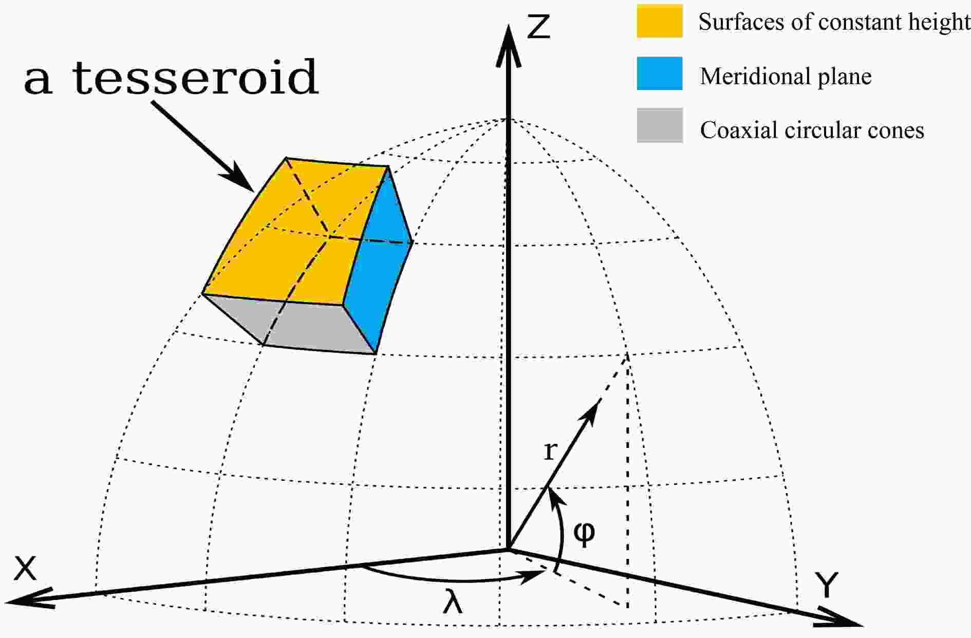
The model is discretized on a global tesseroid grid. Traditional gravity modeling often uses planar approximations and simple geometric elements such as rectangular prisms or point masses to represent density heterogeneity [13, 14]. For global modeling, the curvature of the Earth makes simple planar approximations unsuitable for model discretization. Tesseroids are a type of grid element commonly used in global gravity field modeling and are better suited to representing mass distributions on a curved Earth [13, 15, 16]. A tesseroid can be regarded as a volume element within a spherical shell, bounded by meridians, parallels, and radial boundaries (see Fig. 1) [13, 16]. Because its geometry conforms more closely to Earth's curvature, it is more suitable than regular elements defined in planar coordinates for discretizing global three-dimensional density models.

Figure 1. (color online) Tesseroid Grid Schematic Diagram, adapted from Uieda, 2016 [16].
We use PREM and CRUST1.0 to construct the reference density model and use HMSL-S06 as the source of shear-wave velocity perturbations [7, 17, 18]. The CRUST1.0 model, with a spatial resolution of
$ 1^\circ \times 1^\circ $ , is used to describe the shallow Earth structure. It includes nine layers that represent water, ice, sediments, crustal units, and the uppermost mantle. The density, thickness, and layer top depth of each layer are extracted from the model. Because CRUST1.0 contains zeros and missing values in some regions, vertical continuity across interfaces is enforced during preprocessing. When a NaN or zero density is detected, it is replaced by the nearest valid value at greater depth within the same column, and the layer bottom depths are then recalculated to remove local overlaps. The PREM radial density profile is then expanded onto a global three-dimensional grid. The crust and mantle models are coupled by replacing the shallow PREM intervals with the corresponding CRUST1.0 values. Where the PREM layer geometry is inconsistent with the local crustal base, the deeper interface positions are adjusted to preserve a continuous crust-to-mantle transition and to eliminate local overlap between neighboring layers. The resulting coupled density field is finally exported as a NetCDF three-dimensional base model containing latitude, longitude, layer top depth, and density.Building on the base density model, this study uses the HMSL-S06 model to provide the relative shear wave velocity perturbation field in the deep mantle. The published HMSL-S06 perturbations are first mapped onto the global
$1^\circ \times 1^\circ$ longitude and latitude grid by bilinear interpolation, and then interpolated onto the 199-layer tesseroid grid of the base model in longitude, latitude, and depth. Based on the interpolated relative shear wave velocity perturbation field, cells deeper than 1000 km with perturbations smaller than −1.5% are operationally defined as LLVP regions. The threshold of −1.5% is adopted here to delineate the broad lateral extent of the anomaly in the interpolated model, rather than to serve as a geophysically unique definition of LLVP. Because previous geophysical studies have reported conflicting inferences regarding the density anomaly of LLVP, with some suggesting positive density perturbations and others suggesting negative ones [19−22], this study does not directly convert velocity perturbations into density perturbations. Instead, a uniform positive density perturbation of 1% is applied within the LLVP region, and the resulting updated model is exported as a NetCDF format three-dimensional density dataset. -
The model is discretized on a global tesseroid grid. Traditional gravity modeling often uses planar approximations and simple geometric elements such as rectangular prisms or point masses to represent density heterogeneity [13, 14]. For global modeling, the curvature of the Earth makes simple planar approximations unsuitable for model discretization. Tesseroids are a type of grid element commonly used in global gravity field modeling and are better suited to representing mass distributions on a curved Earth [13, 15, 16]. A tesseroid can be regarded as a volume element within a spherical shell, bounded by meridians, parallels, and radial boundaries (see Fig. 1) [13, 16]. Because its geometry conforms more closely to Earth's curvature, it is more suitable than regular elements defined in planar coordinates for discretizing global three-dimensional density models.
Figure 1. (color online) Tesseroid Grid Schematic Diagram, Adapted from Uieda, 2015 [16].
We use PREM and CRUST1.0 to construct the reference density model and use HMSL-S06 as the source of shear-wave velocity perturbations [7, 17, 18]. The CRUST1.0 model, with a spatial resolution of
$ 1^\circ \times 1^\circ $ , is used to describe the shallow Earth structure. It includes nine layers that represent water, ice, sediments, crustal units, and the uppermost mantle. The density, thickness, and layer top depth of each layer are extracted from the model. Because CRUST1.0 contains zeros and missing values in some regions, vertical continuity across interfaces is enforced during preprocessing. When a NaN or zero density is detected, it is replaced by the nearest valid value at greater depth within the same column, and the layer bottom depths are then recalculated to remove local overlaps. The PREM radial density profile is then expanded onto a global three-dimensional grid. The crust and mantle models are coupled by replacing the shallow PREM intervals with the corresponding CRUST1.0 values. Where the PREM layer geometry is inconsistent with the local crustal base, the deeper interface positions are adjusted to preserve a continuous crust-to-mantle transition and to eliminate local overlap between neighboring layers. The resulting coupled density field is finally exported as a NetCDF three-dimensional base model containing latitude, longitude, layer top depth, and density.Building on the base density model, this study uses the HMSL-S06 model to provide the relative shear wave velocity perturbation field in the deep mantle. The published HMSL-S06 perturbations are first mapped onto the global
$1^\circ \times 1^\circ$ longitude and latitude grid by bilinear interpolation, and then interpolated onto the 199-layer tesseroid grid of the base model in longitude, latitude, and depth. Based on the interpolated relative shear wave velocity perturbation field, cells deeper than 1000 km with perturbations smaller than −1.5% are operationally defined as LLVP regions. The threshold of −1.5% is adopted here to delineate the broad lateral extent of the anomaly in the interpolated model, rather than to serve as a geophysically unique definition of LLVP. Because previous geophysical studies have reported conflicting inferences regarding the density anomaly of LLVP, with some suggesting positive density perturbations and others suggesting negative ones [19−22], this study does not directly convert velocity perturbations into density perturbations. Instead, a uniform positive density perturbation of 1% is applied within the LLVP region, and the resulting updated model is exported as a NetCDF format three-dimensional density dataset. -
S. T. Petcov pointed out that global Earth properties, such as the total mass and moment of inertia, provide important consistency conditions in neutrino studies of Earth's internal structure [23]. In this work, we derive closed-form expressions for the total mass and axial moment of inertia of our 3D Earth density model and evaluate them as global consistency checks.
The Earth density model is discretized into tesseroid cells. Specifically, the globe is represented by
$ 180\times360\times199 $ tesseroids defined on a longitude, latitude, and radial grid, with layer-dependent radial thickness. Each tesseroid is bounded by two meridians, two parallels, and two concentric spherical surfaces of different radii. In this section, we use λ for longitude, φ for latitude, and r for radius, with all angular quantities in the integrals expressed in radians. In the trajectory calculations, θ denotes the zenith angle and ϕ denotes the azimuth angle. In spherical coordinates, the volume element of a tesseroid is$ \begin{array}{l} dV = r^{2}\cos\varphi \, dr \, d\varphi \, d\lambda \end{array} $
(1) Accordingly, for a tesseroid cell bounded by radii
$ r_1 $ to$ r_2 $ , latitudes$ \varphi_1 $ to$ \varphi_2 $ , and longitudes$ \lambda_1 $ to$ \lambda_2 $ , its volume can be expressed as the following triple integral:$ V_{\mathrm{Tesseroids}}=\int_{\lambda_1}^{\lambda_2}\int_{\varphi_1}^{\varphi_2}\int_{r_1}^{r_2} r^2\cos\varphi\,dr\,d\varphi\,d\lambda $
(2) This expression follows the optimization of tesseroid gravity computations in spherical coordinates by Thomas Grombein and co-authors [24]. The analytical solution is:
$ V_{\mathrm{Tesseroids}}=\frac{1}{3}\,(\lambda_2-\lambda_1)(\sin\varphi_2-\sin\varphi_1)(r_2^3-r_1^3) $
(3) Assuming constant density ρ within a cell, the mass of a tesseroid can be obtained by the volume integral:
$ m=\rho\iiint_{V} r^2\cos\varphi\,dr\,d\varphi\,d\lambda $
(4) Summing the mass of all cells yields the total mass
$ M_{\oplus} $ of the model. The total moment of inertia$ I_{\oplus} $ characterizes the distribution of mass inside the Earth. From rigid-body dynamics, a mass element$ \mathrm{d}m $ contributes$ \mathrm{d}I=r_{\perp}^{2}\mathrm{d}m $ about the spin (Z) axis, where$ r_{\perp} $ is the perpendicular distance to the Z axis. In spherical coordinates$ (r,\varphi,\lambda) $ ,$ r_{\perp}=r\cos\varphi $ . Therefore, for a tesseroid of uniform density ρ, the axial moment of inertia is given by:$ I_{\mathrm{Tesseroids}}=\rho\int_{\lambda_1}^{\lambda_2}\int_{\varphi_1}^{\varphi_2}\int_{r_1}^{r_2} r^4\cos^3\varphi\,dr\,d\varphi\,d\lambda $
(5) Evaluating the triple integral yields the closed-form expression:
$ \begin{aligned}[b] I_{\mathrm{Tesseroids}}=\;&\frac{\rho}{5}\,(\lambda_2-\lambda_1)(r_2^{5}-r_1^{5})\\&\times\left(\sin\varphi_2-\sin\varphi_1-\frac{\sin^{3}\varphi_2-\sin^{3}\varphi_1}{3}\right) \end{aligned} $
(6) Finally, the model's total moment of inertia
$ I_{\oplus} $ is obtained by summing$ I_{\mathrm{Tesseroids}} $ over all cells. -
S. T. Petcov pointed out that global Earth properties, such as the total mass and moment of inertia, provide important consistency conditions in neutrino studies of Earth's internal structure [23]. In this work, we derive closed-form expressions for the total mass and axial moment of inertia of our 3D Earth density model and evaluate them as global consistency checks.
The Earth density model is discretized into tesseroid cells. Specifically, the globe is represented by
$ 180\times360\times199 $ tesseroids defined on a longitude, latitude, and radial grid, with layer-dependent radial thickness. Each tesseroid is bounded by two meridians, two parallels, and two concentric spherical surfaces of different radii. In this section, we use λ for longitude, φ for latitude, and r for radius, with all angular quantities in the integrals expressed in radians. In the trajectory calculations, θ denotes the zenith angle and ϕ denotes the azimuth angle. In spherical coordinates, the volume element of a tesseroid is$ \begin{array}{l} {\rm d}V = r^{2}\cos\varphi \, {\rm d}r \, {\rm d}\varphi \, {\rm d}\lambda .\end{array} $
(1) Accordingly, for a tesseroid cell bounded by radii
$ r_1 $ to$ r_2 $ , latitudes$ \varphi_1 $ to$ \varphi_2 $ , and longitudes$ \lambda_1 $ to$ \lambda_2 $ , its volume can be expressed as the following triple integral:$ V_{\mathrm{Tesseroids}}=\int_{\lambda_1}^{\lambda_2}\int_{\varphi_1}^{\varphi_2}\int_{r_1}^{r_2} r^2\cos\varphi\,{\rm d}r\,{\rm d}\varphi\,{\rm d}\lambda. $
(2) This expression follows the optimization of tesseroid gravity computations in spherical coordinates by Thomas Grombein and co-authors [24]. The analytical solution is:
$ V_{\mathrm{Tesseroids}}=\frac{1}{3}\,(\lambda_2-\lambda_1)(\sin\varphi_2-\sin\varphi_1)(r_2^3-r_1^3). $
(3) Assuming constant density ρ within a cell, the mass of a tesseroid can be obtained by the volume integral:
$ m=\rho\iiint_{V} r^2\cos\varphi\,{\rm d}r\,{\rm d}\varphi\,{\rm d}\lambda. $
(4) Summing the mass of all cells yields the total mass
$ M_{\oplus} $ of the model. The total moment of inertia$ I_{\oplus} $ characterizes the distribution of mass inside the Earth. From rigid-body dynamics, a mass element$ \mathrm{d}m $ contributes$ \mathrm{d}I=r_{\perp}^{2}\mathrm{d}m $ about the spin (Z) axis, where$ r_{\perp} $ is the perpendicular distance to the Z axis. In spherical coordinates$ (r,\varphi,\lambda) $ ,$ r_{\perp}=r\cos\varphi $ . Therefore, for a tesseroid of uniform density ρ, the axial moment of inertia is given by:$ I_{\mathrm{Tesseroids}}=\rho\int_{\lambda_1}^{\lambda_2}\int_{\varphi_1}^{\varphi_2}\int_{r_1}^{r_2} r^4\cos^3\varphi\,{\rm d}r\,{\rm d}\varphi\,{\rm d}\lambda .$
(5) Evaluating the triple integral yields the closed-form expression:
$ \begin{aligned}[b] I_{\mathrm{Tesseroids}}=\;&\frac{\rho}{5}\,(\lambda_2-\lambda_1)(r_2^{5}-r_1^{5})\\&\times\left(\sin\varphi_2-\sin\varphi_1-\frac{\sin^{3}\varphi_2-\sin^{3}\varphi_1}{3}\right). \end{aligned} $
(6) Finally, the model's total moment of inertia
$ I_{\oplus} $ is obtained by summing$ I_{\mathrm{Tesseroids}} $ over all cells. -
Neutrino oscillation probabilities depend on the matter density along the path. When the path crosses deep regions such as the mantle and the core, the oscillation pattern changes markedly. Bakhti and colleagues examined trajectory calculations for solar neutrinos in 2020 [5]. Earlier work by Rebekah Pestes and co-authors derived trajectory-path computations on regular grids [6].
To model, with fidelity, the propagation of atmospheric neutrinos through Earth's laterally heterogeneous interior, we adopt a trajectory-tracing algorithm tailored to a 3D model built on tesseroid cells, and we sample the matter density along each path. In the trajectory calculation, Earth is treated as a sphere with a non-uniform surface. We assume that the neutrino travels along a straight line through Earth. The trajectory is determined by the detector location (its latitude, longitude, and depth) and by the arrival direction (zenith angle and azimuth). The geocentric Cartesian coordinates of the detector are given by:
$ \begin{array}{l} \mathbf{P}_d= \begin{bmatrix} r_d\cos\varphi_d\cos\lambda_d \\ r_d\cos\varphi_d\sin\lambda_d \\ r_d\sin\varphi_d \end{bmatrix}. \end{array}$
(7) At the detector location, we set a right-handed local coordinate system with axes pointing due East (E), due North (N), and upward along the local outward normal (U), denoted as (
$ \hat{e}_E,\hat{e}_N,\hat{e}_U $ ). The direction vector is taken as:$ \begin{array}{l} \mathbf{d}_{\mathrm{local}}= \begin{bmatrix} \sin\theta_z\,\sin\phi_z \\ \sin\theta_z\,\cos\phi_z \\ \cos\theta_z \end{bmatrix}. \end{array}$
(8) Here,
$ \theta_z $ is the zenith angle (measured from$ \hat{e}_U $ outward,$ 0\to\pi $ ), and$ \phi_z $ is the azimuth angle (measured from North toward East,$ 0\to2\pi $ ). The ENU basis vectors expressed in the geocentric Cartesian (Earth-Centered, Earth-Fixed; ECEF) frame are:$ \begin{aligned}[b] \hat{e}_E &= \begin{bmatrix} -\sin\lambda_d \\ \cos\lambda_d \\ 0 \end{bmatrix}, \quad \hat{e}_N = \begin{bmatrix} -\sin\varphi_d\cos\lambda_d \\ -\sin\varphi_d\sin\lambda_d \\ \cos\varphi_d \end{bmatrix}, \\ \hat{e}_U &= \begin{bmatrix} \cos\varphi_d\cos\lambda_d \\ \cos\varphi_d\sin\lambda_d \\ \sin\varphi_d \end{bmatrix}. \end{aligned} $
(9) The global direction vector is given by:
$ \begin{array}{l} \mathbf{d}_{\mathrm{global}}=\sin\theta_z\sin\phi_z\,\hat{e}_E+\sin\theta_z\cos\phi_z\,\hat{e}_N+\cos\theta_z\,\hat{e}_U . \end{array}$
(10) The parametric equation of the trajectory is then:
$ \begin{array}{l} \mathbf{Q}(t)=\mathbf{P}_d+t\,\mathbf{d}_{\mathrm{global}}, \qquad t\geqslant 0. \end{array}$
(11) We obtain trajectory information by computing intersections between the path and grid cells. Directly performing exact intersections against millions of cells is too costly, so we accelerate the process with a bounding volume hierarchy (BVH). Before tracing, we compute for each tesseroid cell a minimal axis-aligned bounding box (AABB) that fully contains the curved cell. Using these boxes, we build a static BVH with a recursive median-split strategy.
For a single trajectory, we traverse the BVH to quickly select a small set of candidate cells. At each node, a ray–box intersection test checks whether the particle path can cross the node's spatial region, which greatly reduces the search space. We then perform exact analytic intersection tests only on the selected cells, discarding the boxes and operating on the six curved boundary surfaces of each tesseroid.
To avoid solving a difficult 3D nonlinear system, we introduce a key coordinate reduction: we define the 2D plane spanned by Earth's center, the detector position
$ P_{\rm d} $ , and the incident direction vector$ d_{\rm global} $ , and project all geometry onto this plane. On this plane, the ray becomes one coordinate axis, and the intersections of the six boundary surfaces with the plane reduce to 2D curves (lines, circles, or conics). Intersecting these curves with the axis yields the exact entry and exit points for each cell. After collecting and sorting all intersections, we obtain the particle's piecewise path through the model. For each traversed tesseroid cell, we compute the corresponding path length and assign the cell density to that segment. In the oscillation-probability calculation, each segment is treated as having constant density, and density discontinuities are allowed at cell boundaries.The path length within each traversed cell is then
$ \begin{array}{l} L_{ijk}=\left\Vert \mathbf{Q}(t_{\mathrm{exit}})-\mathbf{Q}(t_{\mathrm{entry}})\right\Vert . \end{array}$
(12) Here,
$ t_{\mathrm{entry}} $ and$ t_{\mathrm{exit}} $ denote the trajectory parameters at the entry and exit points of the cell, respectively, and$ \mathbf{Q}(t) $ is the position vector along the trajectory, as defined in Eq. (11). -
Neutrino oscillation probabilities depend on the matter density along the path. When the path crosses deep regions such as the mantle and the core, the oscillation pattern changes markedly. Bakhti and colleagues examined trajectory calculations for solar neutrinos in 2020 [5]. Earlier work by Rebekah Pestes and co-authors derived trajectory-path computations on regular grids [6].
To model, with fidelity, the propagation of atmospheric neutrinos through Earth's laterally heterogeneous interior, we adopt a trajectory-tracing algorithm tailored to a 3D model built on tesseroid cells, and we sample the matter density along each path. In the trajectory calculation, Earth is treated as a sphere with a non-uniform surface. We assume that the neutrino travels along a straight line through Earth. The trajectory is determined by the detector location (its latitude, longitude, and depth) and by the arrival direction (zenith angle and azimuth). The geocentric Cartesian coordinates of the detector are given by:
$ \begin{array}{l} \mathbf{P}_d= \begin{bmatrix} r_d\cos\varphi_d\cos\lambda_d \\ r_d\cos\varphi_d\sin\lambda_d \\ r_d\sin\varphi_d \end{bmatrix} \end{array}$
(7) At the detector location, we set a right-handed local coordinate system with axes pointing due East (E), due North (N), and upward along the local outward normal (U), denoted as (
$ \hat{e}_E,\hat{e}_N,\hat{e}_U $ ). The direction vector is taken as:$ \begin{array}{l} \mathbf{d}_{\mathrm{local}}= \begin{bmatrix} \sin\theta_z\,\sin\phi_z \\ \sin\theta_z\,\cos\phi_z \\ \cos\theta_z \end{bmatrix} \end{array}$
(8) Here,
$ \theta_z $ is the zenith angle (measured from$ \hat{e}_U $ outward,$ 0\to\pi $ ), and$ \phi_z $ is the azimuth angle (measured from North toward East,$ 0\to2\pi $ ). The ENU basis vectors expressed in the geocentric Cartesian (Earth-Centered, Earth-Fixed; ECEF) frame are:$ \begin{aligned}[b] \hat{e}_E &= \begin{bmatrix} -\sin\lambda_d \\ \cos\lambda_d \\ 0 \end{bmatrix}, \quad \hat{e}_N = \begin{bmatrix} -\sin\varphi_d\cos\lambda_d \\ -\sin\varphi_d\sin\lambda_d \\ \cos\varphi_d \end{bmatrix}, \\ \hat{e}_U &= \begin{bmatrix} \cos\varphi_d\cos\lambda_d \\ \cos\varphi_d\sin\lambda_d \\ \sin\varphi_d \end{bmatrix}. \end{aligned} $
(9) The global direction vector is given by:
$ \begin{array}{l} \mathbf{d}_{\mathrm{global}}=\sin\theta_z\sin\phi_z\,\hat{e}_E+\sin\theta_z\cos\phi_z\,\hat{e}_N+\cos\theta_z\,\hat{e}_U \end{array}$
(10) The parametric equation of the trajectory is then:
$ \begin{array}{l} \mathbf{Q}(t)=\mathbf{P}_d+t\,\mathbf{d}_{\mathrm{global}}, \qquad t\geqslant 0. \end{array}$
(11) We obtain trajectory information by computing intersections between the path and grid cells. Directly performing exact intersections against millions of cells is too costly, so we accelerate the process with a bounding volume hierarchy (BVH). Before tracing, we compute for each tesseroid cell a minimal axis-aligned bounding box (AABB) that fully contains the curved cell. Using these boxes, we build a static BVH with a recursive median-split strategy.
For a single trajectory, we traverse the BVH to quickly select a small set of candidate cells. At each node, a ray–box intersection test checks whether the particle path can cross the node's spatial region, which greatly reduces the search space. We then perform exact analytic intersection tests only on the selected cells, discarding the boxes and operating on the six curved boundary surfaces of each tesseroid.
To avoid solving a difficult 3D nonlinear system, we introduce a key coordinate reduction: we define the 2D plane spanned by Earth's center, the detector position
$ P_d $ , and the incident direction vector$ d_{global} $ , and project all geometry onto this plane. On this plane, the ray becomes one coordinate axis, and the intersections of the six boundary surfaces with the plane reduce to 2D curves (lines, circles, or conics). Intersecting these curves with the axis yields the exact entry and exit points for each cell. After collecting and sorting all intersections, we obtain the particle's piecewise path through the model. For each traversed tesseroid cell, we compute the corresponding path length and assign the cell density to that segment. In the oscillation-probability calculation, each segment is treated as having constant density, and density discontinuities are allowed at cell boundaries.The path length within each traversed cell is then
$ \begin{array}{l} L_{ijk}=\left\Vert \mathbf{Q}(t_{\mathrm{exit}})-\mathbf{Q}(t_{\mathrm{entry}})\right\Vert . \end{array}$
(12) Here,
$ t_{\mathrm{entry}} $ and$ t_{\mathrm{exit}} $ denote the trajectory parameters at the entry and exit points of the cell, respectively, and$ \mathbf{Q}(t) $ is the position vector along the trajectory, as defined in Eq. (11). -
Neutrino oscillation probabilities depend on the matter density along the path. When the path crosses deep regions such as the mantle and the core, the oscillation pattern changes markedly. Bakhti and colleagues examined trajectory calculations for solar neutrinos in 2020 [5]. Earlier work by Rebekah Pestes and co-authors derived trajectory-path computations on regular grids [6].
To model, with fidelity, the propagation of atmospheric neutrinos through Earth's laterally heterogeneous interior, we adopt a trajectory-tracing algorithm tailored to a 3D model built on tesseroid cells, and we sample the matter density along each path. In the trajectory calculation, Earth is treated as a sphere with a non-uniform surface. We assume that the neutrino travels along a straight line through Earth. The trajectory is determined by the detector location (its latitude, longitude, and depth) and by the arrival direction (zenith angle and azimuth). The geocentric Cartesian coordinates of the detector are given by:
$ \begin{array}{l} \mathbf{P}_d= \begin{bmatrix} r_d\cos\varphi_d\cos\lambda_d \\ r_d\cos\varphi_d\sin\lambda_d \\ r_d\sin\varphi_d \end{bmatrix}. \end{array}$
(7) At the detector location, we set a right-handed local coordinate system with axes pointing due East (E), due North (N), and upward along the local outward normal (U), denoted as (
$ \hat{e}_E,\hat{e}_N,\hat{e}_U $ ). The direction vector is taken as:$ \begin{array}{l} \mathbf{d}_{\mathrm{local}}= \begin{bmatrix} \sin\theta_z\,\sin\phi_z \\ \sin\theta_z\,\cos\phi_z \\ \cos\theta_z \end{bmatrix}. \end{array}$
(8) Here,
$ \theta_z $ is the zenith angle (measured from$ \hat{e}_U $ outward,$ 0\to\pi $ ), and$ \phi_z $ is the azimuth angle (measured from North toward East,$ 0\to2\pi $ ). The ENU basis vectors expressed in the geocentric Cartesian (Earth-Centered, Earth-Fixed; ECEF) frame are:$ \begin{aligned}[b] \hat{e}_E &= \begin{bmatrix} -\sin\lambda_d \\ \cos\lambda_d \\ 0 \end{bmatrix}, \quad \hat{e}_N = \begin{bmatrix} -\sin\varphi_d\cos\lambda_d \\ -\sin\varphi_d\sin\lambda_d \\ \cos\varphi_d \end{bmatrix}, \\ \hat{e}_U &= \begin{bmatrix} \cos\varphi_d\cos\lambda_d \\ \cos\varphi_d\sin\lambda_d \\ \sin\varphi_d \end{bmatrix}. \end{aligned} $
(9) The global direction vector is given by:
$ \begin{array}{l} \mathbf{d}_{\mathrm{global}}=\sin\theta_z\sin\phi_z\,\hat{e}_E+\sin\theta_z\cos\phi_z\,\hat{e}_N+\cos\theta_z\,\hat{e}_U . \end{array}$
(10) The parametric equation of the trajectory is then:
$ \begin{array}{l} \mathbf{Q}(t)=\mathbf{P}_d+t\,\mathbf{d}_{\mathrm{global}}, \qquad t\geqslant 0. \end{array}$
(11) We obtain trajectory information by computing intersections between the path and grid cells. Directly performing exact intersections against millions of cells is too costly, so we accelerate the process with a bounding volume hierarchy (BVH). Before tracing, we compute for each tesseroid cell a minimal axis-aligned bounding box (AABB) that fully contains the curved cell. Using these boxes, we build a static BVH with a recursive median-split strategy.
For a single trajectory, we traverse the BVH to quickly select a small set of candidate cells. At each node, a ray–box intersection test checks whether the particle path can cross the node's spatial region, which greatly reduces the search space. We then perform exact analytic intersection tests only on the selected cells, discarding the boxes and operating on the six curved boundary surfaces of each tesseroid.
To avoid solving a difficult 3D nonlinear system, we introduce a key coordinate reduction: we define the 2D plane spanned by Earth's center, the detector position
$ P_{\rm d} $ , and the incident direction vector$ d_{\rm global} $ , and project all geometry onto this plane. On this plane, the ray becomes one coordinate axis, and the intersections of the six boundary surfaces with the plane reduce to 2D curves (lines, circles, or conics). Intersecting these curves with the axis yields the exact entry and exit points for each cell. After collecting and sorting all intersections, we obtain the particle's piecewise path through the model. For each traversed tesseroid cell, we compute the corresponding path length and assign the cell density to that segment. In the oscillation-probability calculation, each segment is treated as having constant density, and density discontinuities are allowed at cell boundaries.The path length within each traversed cell is then
$ \begin{array}{l} L_{ijk}=\left\Vert \mathbf{Q}(t_{\mathrm{exit}})-\mathbf{Q}(t_{\mathrm{entry}})\right\Vert . \end{array}$
(12) Here,
$ t_{\mathrm{entry}} $ and$ t_{\mathrm{exit}} $ denote the trajectory parameters at the entry and exit points of the cell, respectively, and$ \mathbf{Q}(t) $ is the position vector along the trajectory, as defined in Eq. (11). -
The oscillation-probability computation is based on a modified version of the library NuOscProbExact [25]. NuOscProbExact, following Ohlsson and Snellman, is a Python library for computing exact two- and three-flavor neutrino oscillation probabilities for any time-independent Hamiltonian [2]. The oscillation parameters adopt the NuFIT 4.0 normal-ordering (NO) best-fit central values [3]. Let the neutrino energy be E; then the three-flavor Hamiltonian in the k-th constant-density segment is:
$ H_k=\frac{1}{2E}\,U\,\mathrm{diag}(0,\Delta m_{21}^{2},\Delta m_{31}^{2})\,U^{\dagger}+\mathrm{diag}(V_{CC,k},0,0). $
(13) Here, U is the PMNS matrix, and
$ \Delta m_{ij}^{2} $ are the mass-squared differences.$ V_{CC,k}=\sqrt{2}\,G_F\,N_{e,k} $ is the charged-current matter potential in segment k. The electron number density is determined from the mass density sampled along the trajectory,$ \rho_k $ , together with the corresponding$ Y_{e,k} $ , through$ N_{e,k}=\rho_k Y_{e,k}/m_N $ in natural units, where$ m_N $ is the average nucleon mass. In principle, the present calculation framework allows$ Y_e $ to vary from one path segment to another, so a spatially varying distribution of$ Y_e $ can be incorporated directly if needed. In this work, however, we adopt a simplified prescription for convenience. We set$ Y_e=0.50 $ for segments with$ \rho_k<7.6\,\mathrm{g\,cm^{-3}} $ , corresponding to crust and mantle regions, and$ Y_e=0.467 $ for segments with$ \rho_k\geq7.6\,\mathrm{g\,cm^{-3}} $ , corresponding to the core. This choice is used here as a practical approximation for converting mass density into electron number density, rather than as a restriction of the oscillation calculation itself. For antineutrinos, we take$ \delta_{\mathrm{CP}}\to-\delta_{\mathrm{CP}} $ and$ V_{CC,k}\to-V_{CC,k} $ . Discretizing the path into N segments of approximately constant density, the total evolution operator is$ U(E)=\prod_{k=1}^{N}\exp \left[-\,{\rm i}\,H_k(E)\,L_k\right]. $
(14) Where
$ L_k $ is the path length in segment k. The channel probability is$ P_{\alpha\beta}(E) = \left|U_{\beta\alpha}(E)\right|^{2} $ . In practice, we compute the exact segment propagator via the SU(3) matrix exponential on each segment and take the ordered product across segments. The algorithm preserves unitarity and converges consistently with respect to segment length. -
The oscillation-probability computation is based on a modified version of the library NuOscProbExact [25]. NuOscProbExact, following Ohlsson and Snellman, is a Python library for computing exact two- and three-flavor neutrino oscillation probabilities for any time-independent Hamiltonian [2]. The oscillation parameters adopt the NuFIT 4.0 normal-ordering (NO) best-fit central values [3]. Let the neutrino energy be E; then the three-flavor Hamiltonian in the k-th constant-density segment is:
$ H_k=\frac{1}{2E}\,U\,\mathrm{diag}(0,\Delta m_{21}^{2},\Delta m_{31}^{2})\,U^{\dagger}+\mathrm{diag}(V_{CC,k},0,0). $
(13) Here, U is the PMNS matrix, and
$ \Delta m_{ij}^{2} $ are the mass-squared differences.$ V_{CC,k}=\sqrt{2}\,G_F\,N_{e,k} $ is the charged-current matter potential in segment k. The electron number density is determined from the mass density sampled along the trajectory,$ \rho_k $ , together with the corresponding$ Y_{e,k} $ , through$ N_{e,k}=\rho_k Y_{e,k}/m_N $ in natural units, where$ m_N $ is the average nucleon mass. In principle, the present calculation framework allows$ Y_e $ to vary from one path segment to another, so a spatially varying distribution of$ Y_e $ can be incorporated directly if needed. In this work, however, we adopt a simplified prescription for convenience. We set$ Y_e=0.50 $ for segments with$ \rho_k<7.6\,\mathrm{g\,cm^{-3}} $ , corresponding to crust and mantle regions, and$ Y_e=0.467 $ for segments with$ \rho_k\geq7.6\,\mathrm{g\,cm^{-3}} $ , corresponding to the core. This choice is used here as a practical approximation for converting mass density into electron number density, rather than as a restriction of the oscillation calculation itself. For antineutrinos, we take$ \delta_{\mathrm{CP}}\to-\delta_{\mathrm{CP}} $ and$ V_{CC,k}\to-V_{CC,k} $ . Discretizing the path into N segments of approximately constant density, the total evolution operator is$ U(E)=\prod_{k=1}^{N}\exp \left[-\,i\,H_k(E)\,L_k\right], $
(14) Where
$ L_k $ is the path length in segment k. The channel probability is$ P_{\alpha\beta}(E) = \left|U_{\beta\alpha}(E)\right|^{2} $ . In practice, we compute the exact segment propagator via the SU(3) matrix exponential on each segment and take the ordered product across segments. The algorithm preserves unitarity and converges consistently with respect to segment length. -
Using the publicly released Super-Kamiokande analysis-bin data, along with the corresponding nominal no-oscillation Monte Carlo counts and the statistical information on the true neutrino energy and true cosine-zenith distributions within each bin, we compute the bin counts associated with the 3D Earth model within the public SK binning framework and compare them with those from the 1D PREM model. For each analysis bin and neutrino category, the public dataset provides the observed counts, the nominal Monte Carlo counts under several oscillation hypotheses, and information on the true neutrino energy and true cosine-zenith distributions, including the mean, RMS, and five representative quantiles.
For each selected analysis bin, we construct a 5 × 5 sampling grid from the five released quantiles of true neutrino energy and the five released quantiles of true cosine zenith angle. At each sampling node, we evaluate the three-flavor oscillation probability matrix along the corresponding Earth-crossing trajectory. The oscillation probability matrices at all sampling nodes are then simply averaged to obtain the bin-averaged oscillation probability matrix for that bin. The sampling nodes are taken directly from the public SK release, and no additional within-bin weighting scheme is introduced in this work.
After obtaining the averaged oscillation probability matrix for a given bin, we apply it to the publicly released nominal no-oscillation Monte Carlo counts in that bin, classified by incident flavor, and sum the resulting contributions into the analysis channels considered in this work, namely electron-like charged-current, muon-like charged-current, tau charged-current, and neutral-current components. Through this procedure, approximate predicted bin counts for the model can be obtained within the public SK binning framework. These results are used here only for comparative tests between the 3D model and the 1D PREM reference model.
It should be noted that this procedure does not constitute a complete detector-level forward simulation. The public SK release does not provide the full bin-response information or the systematic-response functions required to reproduce the official fit exactly. In addition, in the official analysis, the oscillation probabilities were computed event by event for the Monte Carlo sample, whereas this process cannot be reconstructed exactly using only the publicly released bin-level information. Therefore, the calculation presented here is more appropriately regarded as an approximate bin-level comparison within the public analysis framework, rather than a complete experimental prediction pipeline.
-
The three-dimensional Earth density model constructed in Section 2.1 is illustrated in Figs. 2 and 3. Figure 2 shows the mean density in several depth intervals after weighting by layer thickness. The shallow part of the model exhibits strong lateral heterogeneity associated mainly with the crust and upper mantle, whereas the deeper mantle is comparatively smoother, except in the regions corresponding to the LLVP domains. Figure 3 further shows the density anomalies in the deep mantle beneath the African and Pacific LLVP regions, where the imposed positive density anomalies appear as laterally localized features above the core-mantle boundary.
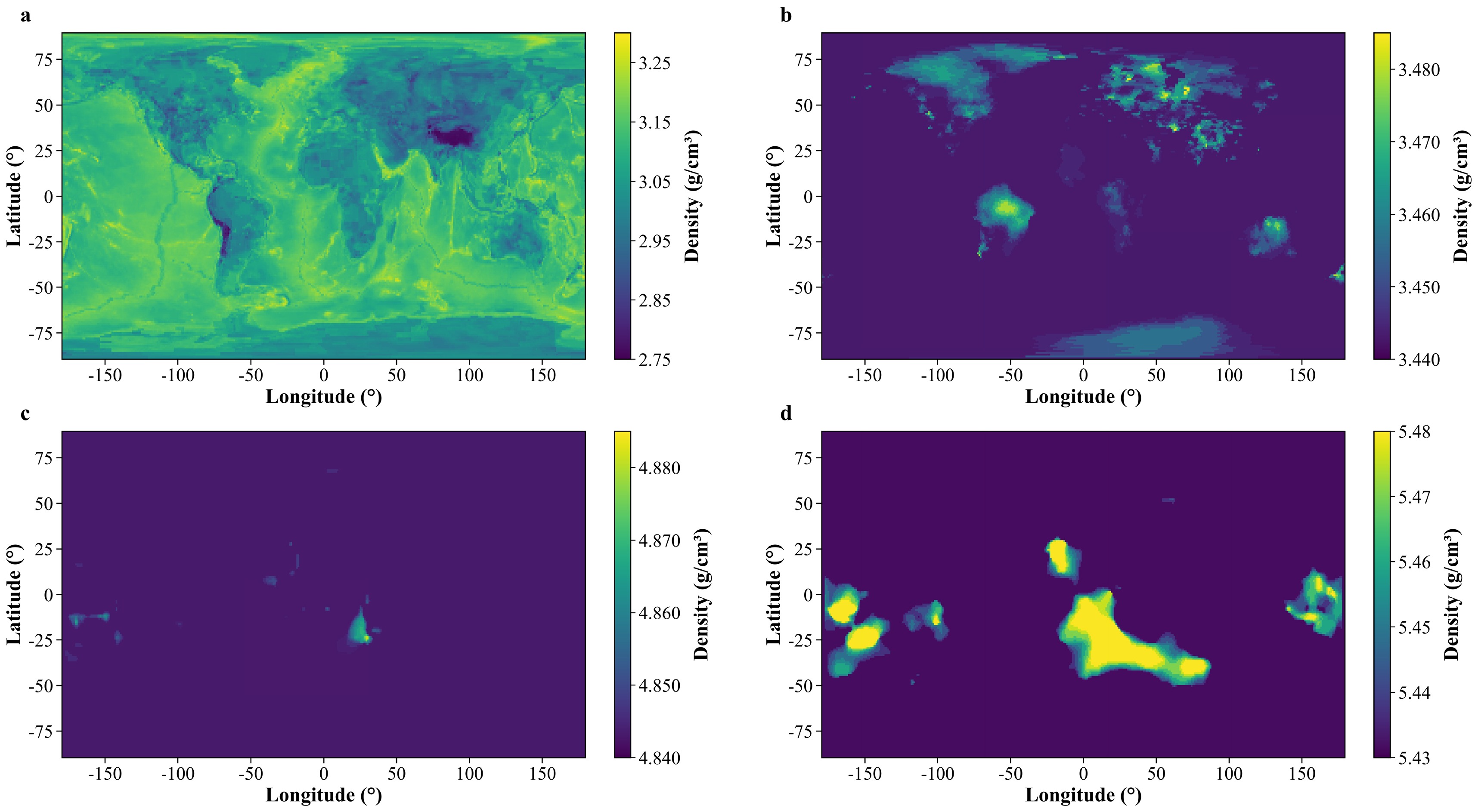
Figure 2. (color online) Thickness-weighted mean density distributions of the three-dimensional Earth density model over different depth ranges are presented. Panels (a)–(d) display the results for 0–60 km, 80–410 km, 1000–2000 km, and 2400–2891 km, respectively.
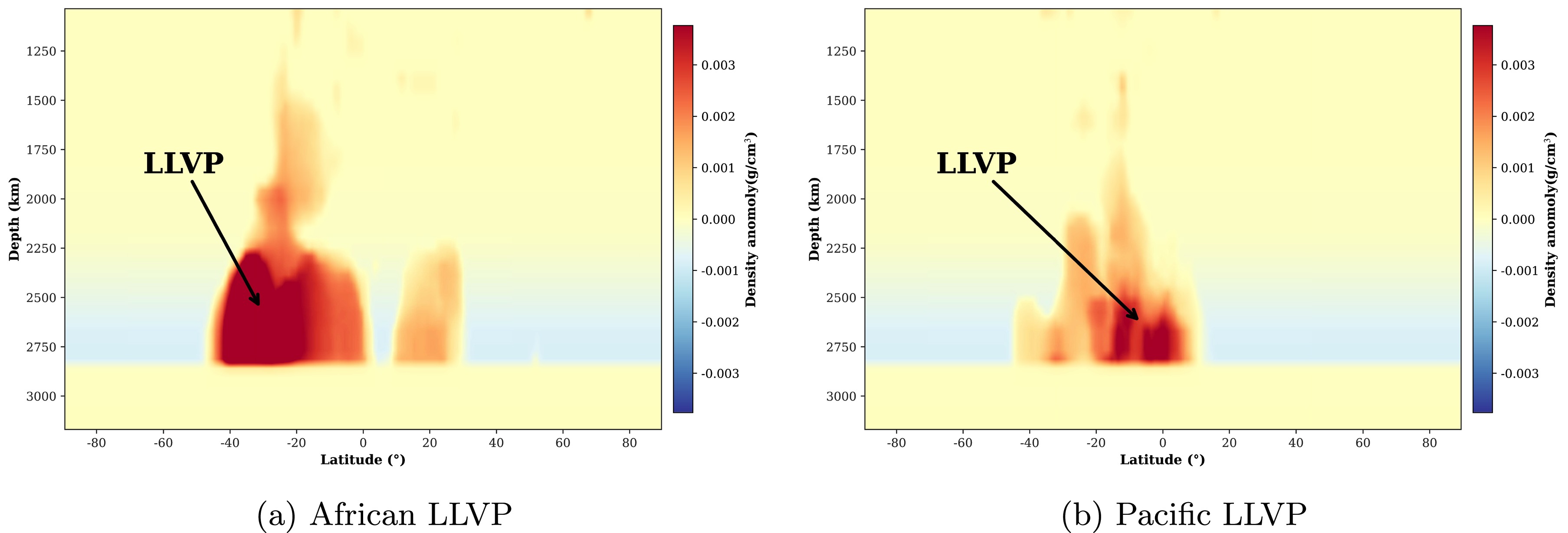
Figure 3. (color online) Latitude and depth sections of density anomaly in the deep mantle for the regions corresponding to the African and Pacific large low shear velocity provinces are presented. Panel (a) shows the section obtained by averaging the density anomaly over the longitude range from 30 degrees west to 60 degrees east, and panel (b) shows the section obtained by averaging the density anomaly over the longitude ranges from 120 degrees east to 180 degrees and from 180 degrees west to 120 degrees west.
The results of these global consistency checks are summarized in Table 1. The total mass and axial moment of inertia derived from the model are both slightly lower than the corresponding geophysical reference values. In Table 1, the reference uncertainty denotes the relative uncertainty associated with each geophysical reference value and is calculated from the uncertainty reported in the source from which the corresponding reference value is adopted [23].
Quantity Model value Reference value Absolute difference Relative error Reference uncertainty Total mass $ 5.957745\times10^{24} $ $ 5.972\times10^{24} $ $ 1.4255\times10^{22} $ $ -0.2387 $ %$ 0.0100 $ %Axial moment of inertia $ 8.008169\times10^{37} $ $ 8.04\times10^{37} $ $ 3.1831\times10^{35} $ $ -0.3959 $ %$ 0.0121 $ %Table 1. Model constraint calculation results.
For the trajectory calculations and oscillation simulations, the detector was placed at the location of the Super-Kamiokande detector, and the zenith angles corresponding to the selected SK analysis bins were used. Figure 4 illustrates a representative case at azimuth
$ 0^{\circ} $ . Panel (a) shows the geocentric radius along the path from the detector to the top of the atmosphere, and panel (b) shows the matter density profile encountered along the trajectory, where the step-like changes mark transitions across major internal boundaries such as the crust, mantle, and core.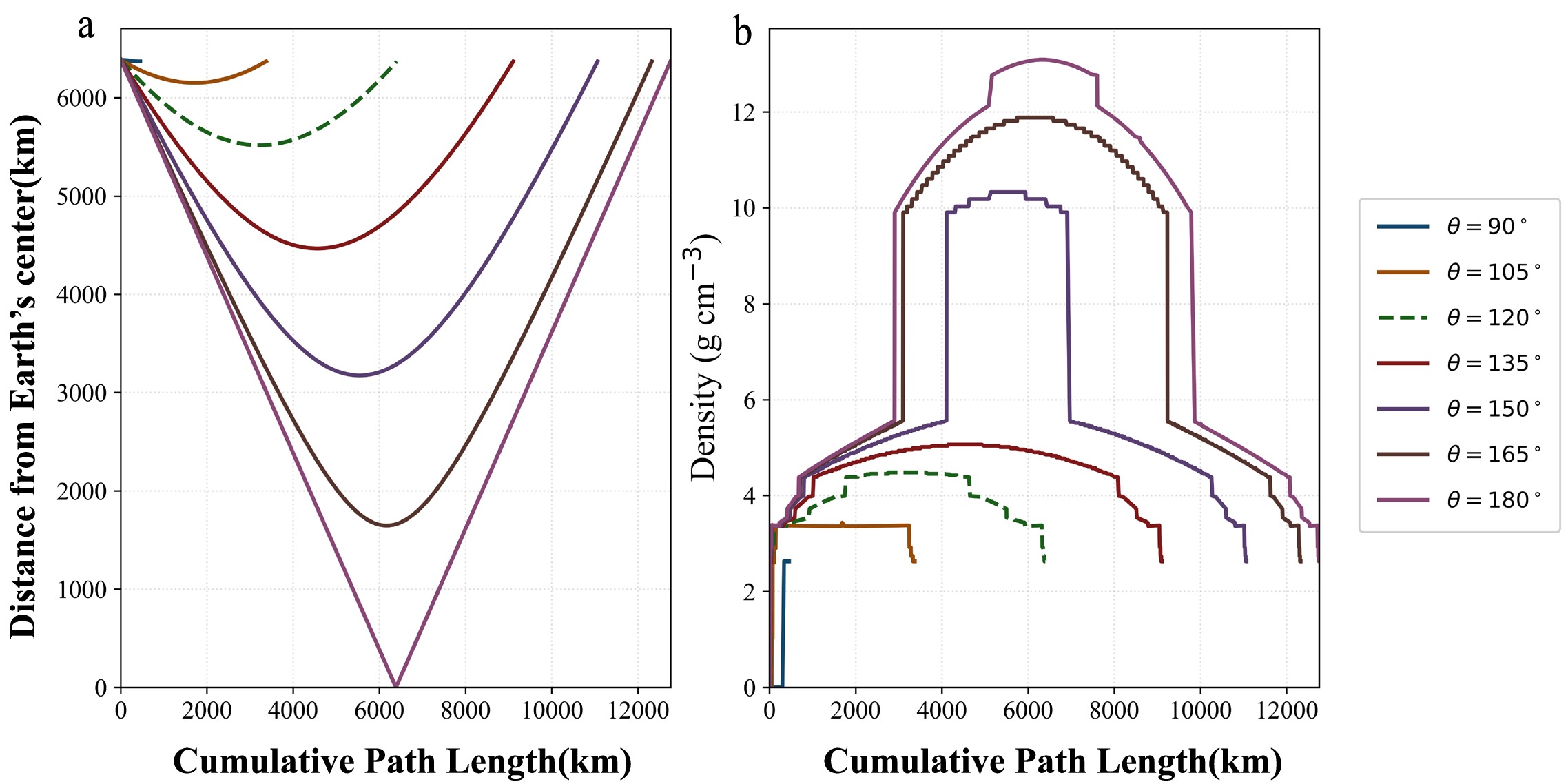
Figure 4. (color online) Geometry and matter profiles of neutrino trajectories at azimuth
$ \phi = 0^{\circ} $ : (a) Distance from Earth's center versus cumulative path length; (b) Matter-density profile along the same trajectories. Curves correspond to the zenith angles θ indicated in the legend (from$ 90^{\circ} $ to$ 180^{\circ} $ ). The azimuth is fixed at$ \phi = 0^{\circ} $ . θ is measured with respect to the local zenith ($ \theta = 180^{\circ} $ : up-going through-Earth paths). Paths start at the detector and terminate at the top of the atmosphere.Along the selected trajectories, we further compute the three-flavor oscillation probabilities as functions of neutrino energy. Figure 5 shows the oscillation probability curves for a representative trajectory at azimuth
$ 0^\circ $ and zenith angle$ 120^\circ $ . The results illustrate the energy-dependent oscillation features for different initial flavor states along the same propagation path.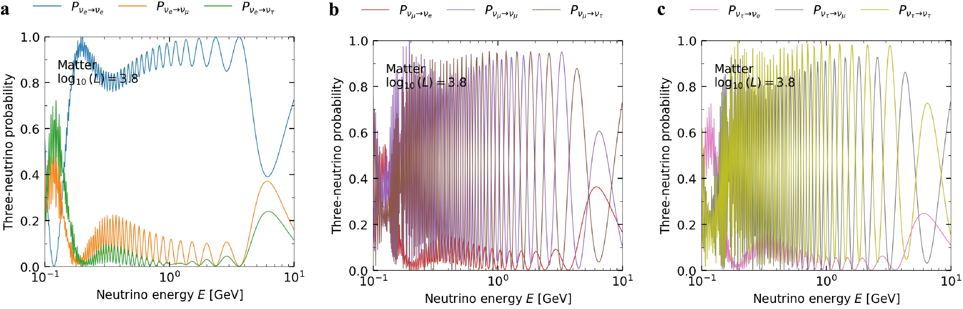
Figure 5. (color online) Three-flavor oscillation probabilities vs. energy at
$ \phi = 0^{\circ} $ ,$ \theta = 120^{\circ} $ under matter effects (normal ordering). (a–c) Panels (a–c) show the three-flavor probabilities$ P_{\nu_\alpha \to \nu_\beta}(E) $ for initial$ \nu_e $ ,$ \nu_\mu $ ,$ \nu_\tau $ , respectively ($ \beta \in \{e, \mu, \tau\} $ ). Probabilities are computed along the trajectory at azimuth$ \phi = 0^{\circ} $ ,$ \theta = 120^{\circ} $ using the path-dependent matter profile, assuming normal mass ordering (NO). The annotation "$ \log_{10}(L) = 3.8 $ " indicates the cumulative path length L along the trajectory (in km, shown on a$ \log_{10} $ scale).Based on the oscillation probability results shown above, we further compare the three-dimensional Earth model with the PREM reference model along the same propagation path. In the two calculations, the neutrino incident direction, path length, and oscillation parameters are kept identical, so the differences arise mainly from the different internal density distributions sampled along the same trajectory. As shown in Fig. 6, the oscillation probability differences between the three-dimensional model and PREM remain small for the representative path considered here. Overall, the probability differences in all channels are mainly at the level of
$ 10^{-4} $ to$ 10^{-3} $ , indicating that the oscillation behavior is still dominated by the radially layered background structure of the Earth.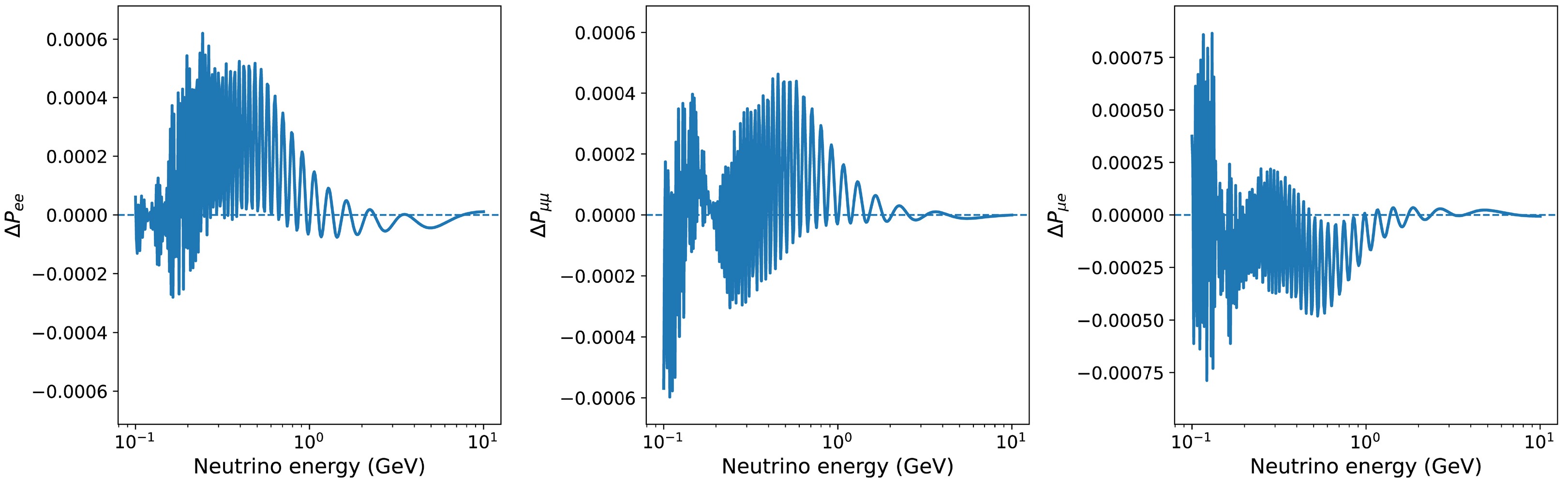
Figure 6. (color online) Differences in representative oscillation probabilities between the three-dimensional Earth model and the PREM reference model for a neutrino trajectory with azimuth
$ 0^\circ $ and zenith angle$ 120^\circ $ . Panels (a)–(c) show$ \Delta P_{ee} $ ,$ \Delta P_{\mu\mu} $ , and$ \Delta P_{\mu e} $ as functions of neutrino energy, respectively.Figure 7 shows the zenith angle distributions of electron-like single-ring events predicted by the three-dimensional model at azimuth
$ 0^\circ $ for different reconstructed momentum bins under the public Super-Kamiokande data binning scheme. Overall, the predicted event counts from the three-dimensional model remain close to those from the PREM reference model, indicating that the differences in the total event distributions between the two models are limited under the calculation method adopted in this work. The distributions vary across reconstructed momentum bins, and the results for the different components show that$ \nu_e $ charged current events provide the dominant contribution, while NC events form a relatively stable background component. These results indicate that the calculation workflow based on the three-dimensional Earth model developed in this work can provide event count predictions that are directly comparable with those from the one-dimensional reference model under the public SK data analysis conditions.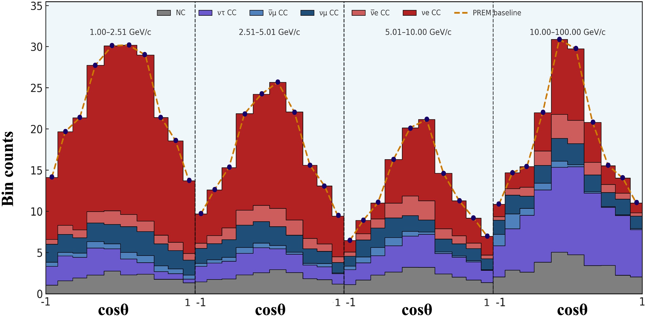
Figure 7. (color online) Zenith angle distributions of electron-like single ring events are predicted by the three-dimensional Earth model at
$ \phi = 0^{\circ} $ for several reconstructed momentum bins. Each panel corresponds to a reconstructed momentum bin indicated in GeV/c. The horizontal axis is$ \cos\theta_z $ , ranging from$ -1 $ to$ 1 $ , and the vertical axis represents the predicted event count in each$ \cos\theta_z $ bin. The colored stacked histograms display the contributions from different interaction channels, including NC,$ \nu_{\tau} $ CC,$ \bar{\nu}_{\mu} $ CC,$ \nu_{\mu} $ CC, and${\nu _e}$ CC. -
The three-dimensional Earth density model constructed in Section 2.1 is illustrated in Figs. 2 and 3. Figure 2 shows the mean density in several depth intervals after weighting by layer thickness. The shallow part of the model exhibits strong lateral heterogeneity associated mainly with the crust and upper mantle, whereas the deeper mantle is comparatively smoother, except in the regions corresponding to the LLVP domains. Figure 3 further shows the density anomalies in the deep mantle beneath the African and Pacific LLVP regions, where the imposed positive density anomalies appear as laterally localized features above the core-mantle boundary.
Figure 2. (color online) Thickness-weighted mean density distributions of the three-dimensional Earth density model over different depth ranges are presented. Panels (a)–(d) display the results for 0–60 km, 80–410 km, 1000–2000 km, and 2400–2891 km, respectively.
Figure 3. (color online) Latitude and depth sections of density anomaly in the deep mantle for the regions corresponding to the African and Pacific large low shear velocity provinces are presented. Panel (a) shows the section obtained by averaging the density anomaly over the longitude range from 30 degrees west to 60 degrees east, and panel (b) shows the section obtained by averaging the density anomaly over the longitude ranges from 120 degrees east to 180 degrees and from 180 degrees west to 120 degrees west.
The results of these global consistency checks are summarized in Table 1. The total mass and axial moment of inertia derived from the model are both slightly lower than the corresponding geophysical reference values. In Table 1, the reference uncertainty denotes the relative uncertainty associated with each geophysical reference value and is calculated from the uncertainty reported in the source from which the corresponding reference value is adopted [23].
Quantity Model value Reference value Absolute difference Relative error Reference uncertainty Total mass $ 5.957745\times10^{24} $ $ 5.972\times10^{24} $ $ 1.4255\times10^{22} $ $ -0.2387 $ %$ 0.0100 $ %Axial moment of inertia $ 8.008169\times10^{37} $ $ 8.04\times10^{37} $ $ 3.1831\times10^{35} $ $ -0.3959 $ %$ 0.0121 $ %Table 1. Model constraint calculation results.
For the trajectory calculations and oscillation simulations, the detector was placed at the location of the Super-Kamiokande detector, and the zenith angles corresponding to the selected SK analysis bins were used. Figure 4 illustrates a representative case at azimuth
$ 0^{\circ} $ . Panel (a) shows the geocentric radius along the path from the detector to the top of the atmosphere, and panel (b) shows the matter density profile encountered along the trajectory, where the step-like changes mark transitions across major internal boundaries such as the crust, mantle, and core.
Figure 4. (color online) Geometry and matter profiles of neutrino trajectories at azimuth
$ \phi = 0^{\circ} $ : (a) Distance from Earth's center versus cumulative path length; (b) Matter-density profile along the same trajectories. Curves correspond to the zenith angles θ indicated in the legend (from$ 90^{\circ} $ to$ 180^{\circ} $ ). The azimuth is fixed at$ \phi = 0^{\circ} $ . θ is measured with respect to the local zenith ($ \theta = 180^{\circ} $ : up-going through-Earth paths). Paths start at the detector and terminate at the top of the atmosphere.Along the selected trajectories, we further compute the three-flavor oscillation probabilities as functions of neutrino energy. Figure 5 shows the oscillation probability curves for a representative trajectory at azimuth
$ 0^\circ $ and zenith angle$ 120^\circ $ . The results illustrate the energy-dependent oscillation features for different initial flavor states along the same propagation path.
Figure 5. (color online) Three-flavor oscillation probabilities vs. energy at
$ \phi = 0^{\circ} $ ,$ \theta = 120^{\circ} $ under matter effects (normal ordering). (a–c) Panels (a–c) show the three-flavor probabilities$ P_{\nu_\alpha \to \nu_\beta}(E) $ for initial$ \nu_e $ ,$ \nu_\mu $ ,$ \nu_\tau $ , respectively ($ \beta \in \{e, \mu, \tau\} $ ). Probabilities are computed along the trajectory at azimuth$ \phi = 0^{\circ} $ ,$ \theta = 120^{\circ} $ using the path-dependent matter profile, assuming normal mass ordering (NO). The annotation "$ \log_{10}(L) = 3.8 $ " indicates the cumulative path length L along the trajectory (in km, shown on a$ \log_{10} $ scale).Based on the oscillation probability results shown above, we further compare the three-dimensional Earth model with the PREM reference model along the same propagation path. In the two calculations, the neutrino incident direction, path length, and oscillation parameters are kept identical, so the differences arise mainly from the different internal density distributions sampled along the same trajectory. As shown in Fig. 6, the oscillation probability differences between the three-dimensional model and PREM remain small for the representative path considered here. Overall, the probability differences in all channels are mainly at the level of
$ 10^{-4} $ to$ 10^{-3} $ , indicating that the oscillation behavior is still dominated by the radially layered background structure of the Earth.
Figure 6. (color online) Differences in representative oscillation probabilities between the three-dimensional Earth model and the PREM reference model for a neutrino trajectory with azimuth
$ 0^\circ $ and zenith angle$ 120^\circ $ . Panels (a)–(c) show$ \Delta P_{ee} $ ,$ \Delta P_{\mu\mu} $ , and$ \Delta P_{\mu e} $ as functions of neutrino energy, respectively.Figure 7 shows the zenith angle distributions of electron-like single-ring events predicted by the three-dimensional model at azimuth
$ 0^\circ $ for different reconstructed momentum bins under the public Super-Kamiokande data binning scheme. Overall, the predicted event counts from the three-dimensional model remain close to those from the PREM reference model, indicating that the differences in the total event distributions between the two models are limited under the calculation method adopted in this work. The distributions vary across reconstructed momentum bins, and the results for the different components show that$ \nu_e $ charged current events provide the dominant contribution, while NC events form a relatively stable background component. These results indicate that the calculation workflow based on the three-dimensional Earth model developed in this work can provide event count predictions that are directly comparable with those from the one-dimensional reference model under the public SK data analysis conditions.
Figure 7. (color online) Zenith angle distributions of electron-like single ring events are predicted by the three-dimensional Earth model at
$ \phi = 0^{\circ} $ for several reconstructed momentum bins. Each panel corresponds to a reconstructed momentum bin indicated in GeV/c. The horizontal axis is$ \cos\theta_z $ , ranging from$ -1 $ to$ 1 $ , and the vertical axis represents the predicted event count in each$ \cos\theta_z $ bin. The colored stacked histograms display the contributions from different interaction channels, including NC,$ \nu_{\tau} $ CC,$ \bar{\nu}_{\mu} $ CC,$ \nu_{\mu} $ CC, and${\nu _e}$ CC. -
The three-dimensional Earth density model constructed in Section 2.1 is illustrated in Figures 2 and 3. Figure 2 shows the mean density in several depth intervals after weighting by layer thickness. The shallow part of the model exhibits strong lateral heterogeneity associated mainly with the crust and upper mantle, whereas the deeper mantle is comparatively smoother, except in the regions corresponding to the LLVP domains. Figure 3 further shows the density anomalies in the deep mantle beneath the African and Pacific LLVP regions, where the imposed positive density anomalies appear as laterally localized features above the core-mantle boundary.
Figure 2. (color online) Thickness-weighted mean density distributions of the three-dimensional Earth density model over different depth ranges are presented. Panels (a)–(d) display the results for 0–60 km, 80–410 km, 1000–2000 km, and 2400–2891 km, respectively.
Figure 3. (color online) Latitude and depth sections of density anomaly in the deep mantle for the regions corresponding to the African and Pacific large low shear velocity provinces are presented. Panel (a) shows the section obtained by averaging the density anomaly over the longitude range from 30 degrees west to 60 degrees east, and panel (b) shows the section obtained by averaging the density anomaly over the longitude ranges from 120 degrees east to 180 degrees and from 180 degrees west to 120 degrees west.
The results of these global consistency checks are summarized in Table 1. The total mass and axial moment of inertia derived from the model are both slightly lower than the corresponding geophysical reference values. In Table 1, the reference uncertainty denotes the relative uncertainty associated with each geophysical reference value and is calculated from the uncertainty reported in the source from which the corresponding reference value is adopted [23].
Quantity Model value Reference value Absolute difference Relative error Reference uncertainty Total mass $ 5.957745\times10^{24} $ $ 5.972\times10^{24} $ $ 1.4255\times10^{22} $ $ -0.2387 $ %$ 0.0100 $ %Axial moment of inertia $ 8.008169\times10^{37} $ $ 8.04\times10^{37} $ $ 3.1831\times10^{35} $ $ -0.3959 $ %$ 0.0121 $ %Table 1. Model constraint calculation results
For the trajectory calculations and oscillation simulations, the detector was placed at the location of the Super-Kamiokande detector, and the zenith angles corresponding to the selected SK analysis bins were used. Figure 4 illustrates a representative case at azimuth
$ 0^{\circ} $ . Panel (a) shows the geocentric radius along the path from the detector to the top of the atmosphere, and panel (b) shows the matter density profile encountered along the trajectory, where the step-like changes mark transitions across major internal boundaries such as the crust, mantle, and core.
Figure 4. (color online) Geometry and matter profiles of neutrino trajectories at azimuth
$ \phi = 0^{\circ} $ : (a) Distance from Earth's center versus cumulative path length; (b) Matter-density profile along the same trajectories. Curves correspond to the zenith angles θ indicated in the legend (from$ 90^{\circ} $ to$ 180^{\circ} $ ). The azimuth is fixed at$ \phi = 0^{\circ} $ . θ is measured with respect to the local zenith ($ \theta = 180^{\circ} $ : up-going through-Earth paths). Paths start at the detector and terminate at the top of the atmosphere.Along the selected trajectories, we further compute the three-flavor oscillation probabilities as functions of neutrino energy. Figure 5 shows the oscillation probability curves for a representative trajectory at azimuth
$ 0^\circ $ and zenith angle$ 120^\circ $ . The results illustrate the energy-dependent oscillation features for different initial flavor states along the same propagation path.
Figure 5. (color online) Three-flavor oscillation probabilities vs. energy at
$ \phi = 0^{\circ} $ ,$ \theta = 120^{\circ} $ under matter effects (normal ordering). (a–c) Panels (a–c) show the three-flavor probabilities$ P_{\nu_\alpha \to \nu_\beta}(E) $ for initial$ \nu_e $ ,$ \nu_\mu $ ,$ \nu_\tau $ , respectively ($ \beta \in \{e, \mu, \tau\} $ ). Probabilities are computed along the trajectory at azimuth$ \phi = 0^{\circ} $ ,$ \theta = 120^{\circ} $ using the path-dependent matter profile, assuming normal mass ordering (NO). The annotation "$ \log_{10}(L) = 3.8 $ " indicates the cumulative path length L along the trajectory (in km, shown on a$ \log_{10} $ scale).Based on the oscillation probability results shown above, we further compare the three-dimensional Earth model with the PREM reference model along the same propagation path. In the two calculations, the neutrino incident direction, path length, and oscillation parameters are kept identical, so the differences arise mainly from the different internal density distributions sampled along the same trajectory. As shown in Fig. 6, the oscillation probability differences between the three-dimensional model and PREM remain small for the representative path considered here. Overall, the probability differences in all channels are mainly at the level of
$ 10^{-4} $ to$ 10^{-3} $ , indicating that the oscillation behavior is still dominated by the radially layered background structure of the Earth.
Figure 6. (color online) Differences in representative oscillation probabilities between the three-dimensional Earth model and the PREM reference model for a neutrino trajectory with azimuth
$ 0^\circ $ and zenith angle$ 120^\circ $ . Panels (a)–(c) show$ \Delta P_{ee} $ ,$ \Delta P_{\mu\mu} $ , and$ \Delta P_{\mu e} $ as functions of neutrino energy, respectively.Figure 7 shows the zenith angle distributions of electron-like single-ring events predicted by the three-dimensional model at azimuth
$ 0^\circ $ for different reconstructed momentum bins under the public Super-Kamiokande data binning scheme. Overall, the predicted event counts from the three-dimensional model remain close to those from the PREM reference model, indicating that the differences in the total event distributions between the two models are limited under the calculation method adopted in this work. The distributions vary across reconstructed momentum bins, and the results for the different components show that$ \nu_e $ charged current events provide the dominant contribution, while NC events form a relatively stable background component. These results indicate that the calculation workflow based on the three-dimensional Earth model developed in this work can provide event count predictions that are directly comparable with those from the one-dimensional reference model under the public SK data analysis conditions.
Figure 7. (color online) Zenith angle distributions of electron-like single ring events are predicted by the three-dimensional Earth model at
$ \phi = 0^{\circ} $ for several reconstructed momentum bins. Each panel corresponds to a reconstructed momentum bin indicated in GeV/c. The horizontal axis is$ \cos\theta_z $ , ranging from$ -1 $ to$ 1 $ , and the vertical axis represents the predicted event count in each$ \cos\theta_z $ bin. The colored stacked histograms display the contributions from different interaction channels, including NC,$ \nu_{\tau} $ CC,$ \bar{\nu}_{\mu} $ CC,$ \nu_{\mu} $ CC, and${\nu _e}$ CC. -
The three-dimensional Earth density model constructed in Section 2.1 is illustrated in Figs. 2 and 3. Figure 2 shows the mean density in several depth intervals after weighting by layer thickness. The shallow part of the model exhibits strong lateral heterogeneity associated mainly with the crust and upper mantle, whereas the deeper mantle is comparatively smoother, except in the regions corresponding to the LLVP domains. Figure 3 further shows the density anomalies in the deep mantle beneath the African and Pacific LLVP regions, where the imposed positive density anomalies appear as laterally localized features above the core-mantle boundary.
Figure 2. (color online) Thickness-weighted mean density distributions of the three-dimensional Earth density model over different depth ranges are presented. Panels (a)–(d) display the results for 0–60 km, 80–410 km, 1000–2000 km, and 2400–2891 km, respectively.
Figure 3. (color online) Latitude and depth sections of density anomaly in the deep mantle for the regions corresponding to the African and Pacific large low shear velocity provinces are presented. Panel (a) shows the section obtained by averaging the density anomaly over the longitude range from 30 degrees west to 60 degrees east, and panel (b) shows the section obtained by averaging the density anomaly over the longitude ranges from 120 degrees east to 180 degrees and from 180 degrees west to 120 degrees west.
The results of these global consistency checks are summarized in Table 1. The total mass and axial moment of inertia derived from the model are both slightly lower than the corresponding geophysical reference values. In Table 1, the reference uncertainty denotes the relative uncertainty associated with each geophysical reference value and is calculated from the uncertainty reported in the source from which the corresponding reference value is adopted [23].
Quantity Model value Reference value Absolute difference Relative error Reference uncertainty Total mass $ 5.957745\times10^{24} $ $ 5.972\times10^{24} $ $ 1.4255\times10^{22} $ $ -0.2387 $ %$ 0.0100 $ %Axial moment of inertia $ 8.008169\times10^{37} $ $ 8.04\times10^{37} $ $ 3.1831\times10^{35} $ $ -0.3959 $ %$ 0.0121 $ %Table 1. Model constraint calculation results.
For the trajectory calculations and oscillation simulations, the detector was placed at the location of the Super-Kamiokande detector, and the zenith angles corresponding to the selected SK analysis bins were used. Figure 4 illustrates a representative case at azimuth
$ 0^{\circ} $ . Panel (a) shows the geocentric radius along the path from the detector to the top of the atmosphere, and panel (b) shows the matter density profile encountered along the trajectory, where the step-like changes mark transitions across major internal boundaries such as the crust, mantle, and core.
Figure 4. (color online) Geometry and matter profiles of neutrino trajectories at azimuth
$ \phi = 0^{\circ} $ : (a) Distance from Earth's center versus cumulative path length; (b) Matter-density profile along the same trajectories. Curves correspond to the zenith angles θ indicated in the legend (from$ 90^{\circ} $ to$ 180^{\circ} $ ). The azimuth is fixed at$ \phi = 0^{\circ} $ . θ is measured with respect to the local zenith ($ \theta = 180^{\circ} $ : up-going through-Earth paths). Paths start at the detector and terminate at the top of the atmosphere.Along the selected trajectories, we further compute the three-flavor oscillation probabilities as functions of neutrino energy. Figure 5 shows the oscillation probability curves for a representative trajectory at azimuth
$ 0^\circ $ and zenith angle$ 120^\circ $ . The results illustrate the energy-dependent oscillation features for different initial flavor states along the same propagation path.
Figure 5. (color online) Three-flavor oscillation probabilities vs. energy at
$ \phi = 0^{\circ} $ ,$ \theta = 120^{\circ} $ under matter effects (normal ordering). (a–c) Panels (a–c) show the three-flavor probabilities$ P_{\nu_\alpha \to \nu_\beta}(E) $ for initial$ \nu_e $ ,$ \nu_\mu $ ,$ \nu_\tau $ , respectively ($ \beta \in \{e, \mu, \tau\} $ ). Probabilities are computed along the trajectory at azimuth$ \phi = 0^{\circ} $ ,$ \theta = 120^{\circ} $ using the path-dependent matter profile, assuming normal mass ordering (NO). The annotation "$ \log_{10}(L) = 3.8 $ " indicates the cumulative path length L along the trajectory (in km, shown on a$ \log_{10} $ scale).Based on the oscillation probability results shown above, we further compare the three-dimensional Earth model with the PREM reference model along the same propagation path. In the two calculations, the neutrino incident direction, path length, and oscillation parameters are kept identical, so the differences arise mainly from the different internal density distributions sampled along the same trajectory. As shown in Fig. 6, the oscillation probability differences between the three-dimensional model and PREM remain small for the representative path considered here. Overall, the probability differences in all channels are mainly at the level of
$ 10^{-4} $ to$ 10^{-3} $ , indicating that the oscillation behavior is still dominated by the radially layered background structure of the Earth.
Figure 6. (color online) Differences in representative oscillation probabilities between the three-dimensional Earth model and the PREM reference model for a neutrino trajectory with azimuth
$ 0^\circ $ and zenith angle$ 120^\circ $ . Panels (a)–(c) show$ \Delta P_{ee} $ ,$ \Delta P_{\mu\mu} $ , and$ \Delta P_{\mu e} $ as functions of neutrino energy, respectively.Figure 7 shows the zenith angle distributions of electron-like single-ring events predicted by the three-dimensional model at azimuth
$ 0^\circ $ for different reconstructed momentum bins under the public Super-Kamiokande data binning scheme. Overall, the predicted event counts from the three-dimensional model remain close to those from the PREM reference model, indicating that the differences in the total event distributions between the two models are limited under the calculation method adopted in this work. The distributions vary across reconstructed momentum bins, and the results for the different components show that$ \nu_e $ charged current events provide the dominant contribution, while NC events form a relatively stable background component. These results indicate that the calculation workflow based on the three-dimensional Earth model developed in this work can provide event count predictions that are directly comparable with those from the one-dimensional reference model under the public SK data analysis conditions.
Figure 7. (color online) Zenith angle distributions of electron-like single ring events are predicted by the three-dimensional Earth model at
$ \phi = 0^{\circ} $ for several reconstructed momentum bins. Each panel corresponds to a reconstructed momentum bin indicated in GeV/c. The horizontal axis is$ \cos\theta_z $ , ranging from$ -1 $ to$ 1 $ , and the vertical axis represents the predicted event count in each$ \cos\theta_z $ bin. The colored stacked histograms display the contributions from different interaction channels, including NC,$ \nu_{\tau} $ CC,$ \bar{\nu}_{\mu} $ CC,$ \nu_{\mu} $ CC, and${\nu _e}$ CC. -
This study introduces the tesseroid grid, which is widely used in gravity inversion, into the problem of atmospheric neutrinos and constructs a three-dimensional initial density model for neutrino Earth tomography. Within this discrete framework, we derive explicit expressions for the total mass and axial moment of inertia of the model. We further develop a corresponding procedure for extracting neutrino trajectory information, so that the density distribution sampled along each trajectory and the associated path length can be recorded within a unified framework. Combined with an energy, zenith angle, and azimuth sampling scheme compatible with three-flavor oscillation calculations and the Super Kamiokande binning scheme, this framework is used to calculate and compare oscillation probabilities and event counts between the three-dimensional model and the one-dimensional reference model. The results show that the three-dimensional model can preserve lateral density heterogeneity while remaining physically consistent overall and can provide oscillation probability and event count results that are directly comparable with those of the traditional one-dimensional spherically symmetric model. The present work should therefore be regarded mainly as a methodological demonstration for future studies of neutrino Earth tomography.
Compared with traditional one-dimensional spherically symmetric models, the three-dimensional density model developed in this study combines multiple sources of Earth structure information and includes the deep mantle heterogeneity considered in the present work. The tesseroid grid construction adopted here originates from gravity studies and provides a flexible discretized framework for later refinement. In future work, regional density information obtained from gravity inversion or other geophysical constraints can be incorporated into the present model in a spatially localized way. Since the radial thickness differs among tesseroid cells, the framework also allows structural detail to be added progressively through the integration of existing regional density models.
Early studies of neutrino Earth tomography largely adopted one-dimensional spherically symmetric Earth models [26−33]. As research methods developed, some studies began to consider non-spherical three-dimensional structure. For example, in solar neutrino studies, previous work showed that the use of a three-dimensional Earth model can change the zenith-related angular distribution of observables such as the day-night asymmetry [5]. Pestes et al. explored three-dimensional neutrino tomography on a regular grid, but their method is less suitable for models with non-uniform grid spacing, and global physical consistency checks were not incorporated into a unified calculation workflow [6]. In contrast, this study establishes a unified tesseroid-based calculation workflow that connects model construction, trajectory extraction, oscillation calculation, and event count comparison. At the same time, the results obtained here also indicate that, under the present calculation scheme, the differences between the three-dimensional model and the one-dimensional reference model remain limited overall. Therefore, the main significance of the present work at this stage lies in providing a technical basis for future model refinement and comparative studies.
In the event count calculations presented in this work, we compare the predictions from the three-dimensional density model with those from the one-dimensional reference model. The results indicate that, within the present calculation scheme, the differences between the three-dimensional and one-dimensional models remain limited overall. For trajectory computation, although a bounding volume hierarchy method is used to accelerate the calculation for individual propagation paths, computational time and memory demand may still become limiting factors when finer grids are adopted or when large-scale uncertainty analyses are performed. Further improvements in parallel computation and code optimization are therefore still needed. For the oscillation parameters, we mainly adopt the best-fit central values from NuFIT 4.0 [3], although these parameters themselves still carry experimental uncertainties. In addition, substantial theoretical and experimental uncertainties remain in atmospheric neutrino flux models and neutrino-nucleon interaction cross sections. We have not yet systematically evaluated how these uncertainties propagate through the present calculation chain and affect the comparison of model results, and this should be addressed in future quantitative analyses. In the oscillation probability calculations, because a precise global profile of electron number density is not yet available, we use mass density as an approximate proxy for electron number density by dividing the density range into several intervals and assigning a corresponding electron number density to each interval. This treatment serves as a practical baseline approximation in the present calculations, but higher precision studies will require more refined prior constraints or smoothing treatments, together with further tests of robustness.
-
This study introduces the tesseroid grid, which is widely used in gravity inversion, into the problem of atmospheric neutrinos and constructs a three-dimensional initial density model for neutrino Earth tomography. Within this discrete framework, we derive explicit expressions for the total mass and axial moment of inertia of the model. We further develop a corresponding procedure for extracting neutrino trajectory information, so that the density distribution sampled along each trajectory and the associated path length can be recorded within a unified framework. Combined with an energy, zenith angle, and azimuth sampling scheme compatible with three-flavor oscillation calculations and the Super Kamiokande binning scheme, this framework is used to calculate and compare oscillation probabilities and event counts between the three-dimensional model and the one-dimensional reference model. The results show that the three-dimensional model can preserve lateral density heterogeneity while remaining physically consistent overall and can provide oscillation probability and event count results that are directly comparable with those of the traditional one-dimensional spherically symmetric model. The present work should therefore be regarded mainly as a methodological demonstration for future studies of neutrino Earth tomography.
Compared with traditional one-dimensional spherically symmetric models, the three-dimensional density model developed in this study combines multiple sources of Earth structure information and includes the deep mantle heterogeneity considered in the present work. The tesseroid grid construction adopted here originates from gravity studies and provides a flexible discretized framework for later refinement. In future work, regional density information obtained from gravity inversion or other geophysical constraints can be incorporated into the present model in a spatially localized way. Since the radial thickness differs among tesseroid cells, the framework also allows structural detail to be added progressively through the integration of existing regional density models.
Early studies of neutrino Earth tomography largely adopted one-dimensional spherically symmetric Earth models [26−33]. As research methods developed, some studies began to consider non-spherical three-dimensional structure. For example, in solar neutrino studies, previous work showed that the use of a three-dimensional Earth model can change the zenith-related angular distribution of observables such as the day-night asymmetry [5]. Pestes et al. explored three-dimensional neutrino tomography on a regular grid, but their method is less suitable for models with non-uniform grid spacing, and global physical consistency checks were not incorporated into a unified calculation workflow [6]. In contrast, this study establishes a unified tesseroid-based calculation workflow that connects model construction, trajectory extraction, oscillation calculation, and event count comparison. At the same time, the results obtained here also indicate that, under the present calculation scheme, the differences between the three-dimensional model and the one-dimensional reference model remain limited overall. Therefore, the main significance of the present work at this stage lies in providing a technical basis for future model refinement and comparative studies.
In the event count calculations presented in this work, we compare the predictions from the three-dimensional density model with those from the one-dimensional reference model. The results indicate that, within the present calculation scheme, the differences between the three-dimensional and one-dimensional models remain limited overall. For trajectory computation, although a bounding volume hierarchy method is used to accelerate the calculation for individual propagation paths, computational time and memory demand may still become limiting factors when finer grids are adopted or when large-scale uncertainty analyses are performed. Further improvements in parallel computation and code optimization are therefore still needed. For the oscillation parameters, we mainly adopt the best-fit central values from NuFIT 4.0 [3], although these parameters themselves still carry experimental uncertainties. In addition, substantial theoretical and experimental uncertainties remain in atmospheric neutrino flux models and neutrino-nucleon interaction cross sections. We have not yet systematically evaluated how these uncertainties propagate through the present calculation chain and affect the comparison of model results, and this should be addressed in future quantitative analyses. In the oscillation probability calculations, because a precise global profile of electron number density is not yet available, we use mass density as an approximate proxy for electron number density by dividing the density range into several intervals and assigning a corresponding electron number density to each interval. This treatment serves as a practical baseline approximation in the present calculations, but higher precision studies will require more refined prior constraints or smoothing treatments, together with further tests of robustness.
Neutrino tomography with a three-dimensional model of Earth's density
- Received Date: 2025-12-25
- Available Online: 2026-07-15
Abstract: Neutrino Earth tomography provides an observational approach to studying the Earth's deep three-dimensional structure that is distinct from seismology. However, most existing studies still rely on one-dimensional density models and therefore cannot adequately represent lateral heterogeneity within the Earth. To address this issue, this study integrates PREM, CRUST1.0, and HMSL-S06 on a tesseroid grid to construct a non-spherically symmetric three-dimensional Earth density model that includes large low-velocity provinces (LLVPs) in the deep mantle. We also develop a corresponding procedure for extracting neutrino propagation trajectories and derive closed-form expressions for the total mass and axial moment of inertia of the discrete model, which are used as global consistency checks. Within an exact three-flavor oscillation framework, we use public Super-Kamiokande data products to compare the event counts predicted by the three-dimensional model with those from a conventional one-dimensional spherically symmetric model. The results show that, under the present calculation scheme, the differences in the overall event count distributions between the three-dimensional model and the one-dimensional reference model remain limited. This study establishes a three-dimensional calculation framework that can provide a methodological basis for future investigations of how lateral density heterogeneity may affect atmospheric neutrino propagation.


 DownLoad: