


 Abstract
 HTML
HTML Reference
 Related
 PDF
PDF



-
Since the discovery of late-time acceleration in the late 90s by Riess [1] and Perlmutter [2], it has been clear that Einstein's cosmological constant must be non-zero to explain late-time de Sitter type expansion. Moreover, studies of the galactic halo and structure formation, as well as baryonic acoustic oscillation (BAO) data, have revealed the existence of dark matter, which is weakly interacting, cold, and non-baryonic [3, 4]. Therefore, the period from the late 90s to the early 2000s was dominated by ΛCDM cosmology, in which dark energy (responsible for late time acceleration) is given by the cosmological constant (Λ) and dark matter (matter responsible for the galactic rotation curve anomaly) is cold and non-baryonic.
The standard model of cosmology, ΛCDM, is one of the most successful models and explains almost all present and past observations with only six free parameters. Although the ΛCDM paradigm is successful, there are still unanswered questions that raise doubts about standard cosmology. First, there is no way of explaining Λ in the standard cosmological model, even though identifying it with dark energy offers remarkable observational tests. For example, if one attempts to explain Λ (the cosmological constant) as simply vacuum energy, a serious problem occurs: a discrepancy on the order of
$ 10^{120} $ is found between the observed value of Λ and the theoretical prediction obtained using one-loop corrections in QFT. To explain dark energy, one must use a scalar field (a quintessence field), which can explain the origin of Λ and why the cosmological constant is so small. There is an alternative method of explaining dark energy or late-time acceleration by modifying Einstein's theory of relativity. It is well known that standard general relativity (GR) is a classical theory and therefore breaks down in extreme-curvature regions, such as near singularities. To avoid this, one must quantize the theory, as in electromagnetism, to obtain a quantum theory of gravity. However, it is also well known that, despite numerous proposals, such as string theory and loop quantum gravity, a comprehensive theory of quantum gravity (that can be experimentally or observationally tested) remains elusive [5, 6]. Athough we cannot find a full quantum gravity theory, we can make some reasonable guesses about how the Einstein-Hilbert action changes while maintaining diffeomorphism symmetry. Regarding CDM, the constituents of dark matter are not fully understood (in this study, we consider Chaplygin gas, which can explain both dark energy and dark matter in a unified framework of matter). Additionally, there is a growing concern in contemporary cosmology regarding Hubble ($ H_0 $ ) tension [7] and$ \sigma_8 $ [8]. Generally, these tensions indicate that our understanding of the full timescale of the universe is limited; that is, contemporary observations do not match those of the early and late universes, which challenges the current ΛCDM model profoundly.One reason for such an anomaly is the importance of quantum effects in explaining the cosmological constant and dark matter. However, because no full quantum gravity theory exists, we can instead note the possible infrared behavior of quantum gravity theory. One loop correction of the graviton-graviton interaction can give rise to the
$ R^2 $ term in the Einstein-Hilbert action, which has been used by Starobinsky [9] to predict inflation in the early universe. Therefore, modified gravity (MOG) is a lucrative alternative for explaining not only dark energy but also various other astrophysical phenomena (such as the super-Chandrasekhar mass limit [10] and black hole accretion [11]). The standard approach to modifying gravity is to modify the Einstein-Hilbert action with a suitable diffeomorphism-invariant scale and then derive the modified equation by varying the metric. Subsequently, a suitable metric (in this case, the Friedmann-Lemaitre-Robertson-Walker (FLRW) metric) can be inserted into the field equation to obtain the modified Einstein equations.In this study, we consider
$ f(Q) $ gravity, a version of MOG based on non-metricity ($ \nabla_{\lambda}g_{\mu\nu}\neq0 $ ) that reduces to GR in the linear limit. Although the actual origin of using non-metricity to unify electromagnetism and gravity dates back to the idea of Weyl, the modern version of$ f(Q) $ cosmology was first proposed by Jimenez et al. [12] and later expanded by them [13, 14]. There are various papers that discuss the data analysis of cosmological models based on$ f(Q) $ gravity in detail [15−20]. Moreover, there has been active effort to analytically study dark energy in the context of$ f(Q) $ gravity via dynamical system analysis [21, 22]. Note that the$ f(Q) $ MOG theory has shown remarkable consistency across various astrophysical objects, such as black holes [23], wormholes [24, 25], and gravastars [26, 27]. In this study, we consider Chaplygin gas as our matter source. Chaplygin gas has long been one of the most prominent candidates for dark energy. Section-II explains several reasons for this, such as the microscopical Chaplygin gas that arises naturally in string theory. The Chaplygin gas equation of state can also be naturally constructed using scalar and DBI fields, as well as brane compactification. On the phenomenological side, Chaplygin gas is not only consistent with current observations but can also provide a natural transition from matter to a dark-energy-dominated universe. Therefore, we use the most general equation of state for Chaplygin gas, which is given by$ p=\alpha \rho+ \beta\rho^m $ .Extensive studies have been conducted on the (non-gravitational) interaction between dark energy and dark matter over the past few decades. A standard quantum field theoretical approach is to consider the quintessence scalar field, whose effective mass becomes comparable to that of dark matter particles, to lead to an exchange of energy between the two components [28, 29]. There are several ways to model this interaction in the continuity equation, but the most simplistic and phenomenologically consistent method is via
$ {\cal{I}} \propto H\rho $ . This encodes the FLRW geometry, which involves dilution via a factor of H and is also consistent with the standard continuity equation. Such a model of the interaction between dark sectors has been widely used in the standard literature [30−32]. The interaction term relieves the tension between dark matter and dark energy, because an analysis with only Bose-Einstein condensation (BEC) dark matter yields$ m=2 $ , as investigated in detail in our previous study [33]. However, there is also an explicit dark energy component that is highly consistent with generalized Chaplygin gas, given as$ m<0 $ . Therefore, the presence of the interaction term provides a unified and physically motivated mechanism through which both branches emerge as viable solutions, with their relative relevance determined by observational constraints rather than imposed assumptions.As previously mentioned, even though Chaplygin gas can effectively explain dark energy, it falls short in explaining dark matter. In this study, we consider dark matter as an effective Bose-Einstein condensate scalar field. There are two primary reasons for this, as explained in Section III. First, the Bose-Einstein condensate is a highly lucrative option for dark matter owing to its lack of viscosity, which may explain why galactic halos have uniform density. It is also visible from the microscopic perspective because the Gross-Pitaevskii equation for a moderately interacting dilute Bose gas can naturally provide an equation of state of the form
$ p=\alpha\rho+\beta\rho^2 $ , which is essentially Chaplygin gas with$ m=2 $ . Beyond the microscopic and phenomenological motivations, our study provides a unified framework that can be used to explain both dark energy and dark matter. We also include an interacting term,$ {\cal{I}}=3H^2\rho $ , which facilitates a transition between dark matter and dark energy.We perform Markov Chain Monte Carlo (MCMC) analysis using Hubble and Pantheon+ SH0ES data and test the model using two of the most popular statistical tests: the AIC and BIC. We also perform the so-called null test for ΛCDM cosmology using statefinder and Om diagnostics.
-
Since the discovery of late-time acceleration in the late 90's, by A. G. Riess [1] and S. Perlmutter [2], it has been clear that Einstein's cosmological constant has to be non-zero in order to explain the late-time de Sitter type expansion. It has also been observed from studies of the galactic halo and structure formation, as well as Baryonic Acoustic Oscillation (BAO) data, that there is dark matter which is weakly interacting, cold, and non-baryonic in nature [3, 4]. So, from the late 90's to the early 2000's was dominated by ΛCDM cosmology, that is, the dark energy (responsible for the late time acceleration) is given by the cosmological constant (Λ) and the dark matter (matter responsible for galactic rotation curve anomaly) is cold and non-baryonic in nature.
The standard model of cosmology, ΛCDM, is one of the most successful models, explaining almost all present and past observations with only six free parameters. Although the ΛCDM paradigm is successful, there are still unanswered questions that raise doubts about standard cosmology. For starters, there is no way to explain Λ in the standard cosmological model, even though identifying it with dark energy gives remarkable observational tests. For example, if one tries to explain Λ (the cosmological constant) as just vacuum energy, one runs into a serious problem: the observed value of Λ versus the theoretical prediction using one-loop corrections in QFT shows a discrepancy of order
$ 10^{120} $ . In order to explain dark energy, one has to use some sort of scalar field (a quintessence field), which can explain the origin of Λ and hence why the cosmological constant is so small. There is an alternative way to explain dark energy or late-time acceleration by modifying Einstein's theory of relativity. It is well known that standard GR is a classical theory, so it breaks down in extreme-curvature regions such as near singularities. Thus, to avoid this, one must quantize the theory, just like electromagnetism, to find a quantum theory of gravity. However, it is also well known that, despite numerous proposals, such as string theory and loop quantum gravity (to name a few), a comprehensive theory of quantum gravity (which can be tested experimentally or observationally) remains elusive [5, 6]. So, noting that even though we cannot find a full quantum gravity theory, one can still make some reasonable guesses about how the Einstein-Hilbert action would change while maintaining diffeomorphism symmetry. As for CDM, we do not have a clear idea what dark matter consists of. (In this article, we have considered the Chaplygin gas, which can explain both dark energy and dark matter in a unified framework of matter.) Apart from these, there is also a growing concern regarding contemporary cosmology about the Hubble ($ H_0 $ ) tension [7] and$ \sigma_8 $ [8]. Roughly speaking, these tensions indicate that our understanding of the full timescale of the universe is limited; that is, contemporary observations do not match those of the early universe and late universe, which challenges the current ΛCDM model in a profound way.It is well understood that one reason for such an anomaly is that the quantum effects become quite important in explaining the cosmological constant or dark matter. However, since we do not have a full quantum gravity theory, we can roughly argue by noting how the infrared behavior of quantum gravity theory might be. It can be seen that one loop correction of the graviton-graviton interaction can give rise to the
$ R^2 $ term in the Einstein-Hilbert action, which has been used by Starobinsky [9] to predict inflation in the early universe. So, modified gravity is a very lucrative alternative to explain not just dark energy, but it can also be used for explaining various other astrophysical phenomena (such as the super-Chandrasekhar mass limit [10], black hole accretion [11], etc.). When it comes to modifying gravity, the standard approach is to modify the Einstein-Hilbert action with a suitable diffeomorphism-invariant scale and then derive the modified equation by varying the metric. From there, one can put a suitable metric (in this case, the FLRW metric) into the field equation to get the modified Einstein equations.In this article, we consider
$ f(Q) $ gravity, a version of modified gravity based on non-metricity ($ \nabla_{\lambda}g_{\mu\nu}\neq0 $ ) and reducing to GR in the linear limit. Although the actual origin of using non-metricity to unify electromagnetism and gravity goes back to the idea of Weyl, the modern version of$ f(Q) $ cosmology was first written by Jimenez et al. [12] and later expanded by them [13, 14]. There are various papers that discuss data analysis in detail for cosmological models based on$ f(Q) $ gravity [15−20]. There has been an active effort to analytically study the dark energy in the context of$ f(Q) $ gravity via dynamical system analysis [21, 22]. It is also worth noting that the modified$ f(Q) $ gravity theory has shown remarkable consistency in various astrophysical objects, such as black holes [23], wormholes [24, 25], and gravastars [26, 27], as well. In this article, we have taken the Chaplygin gas as our matter source. Chaplygin gas has been one of the most prominent candidates for dark energy for a very long time. There are several reasons for that, as we will discuss in Section-II, such as the microscopically Chaplygin gas that arises very naturally in string theory. There is also a very natural way to construct the Chaplygin gas equation of state using a scalar field and a DBI field, and also by Brane compactification. On the phenomenological side, the Chaplygin gas is not just consistent with the current observation, but it can also give a very natural transition from matter to a dark-energy-dominated universe. So, here we have taken the most general equation of state of the Chaplygin gas, which is given by$ p=\alpha \rho+ \beta\rho^m $ .There has been a lot of study regarding the interaction (non-gravitational) between dark energy and dark matter over the past few decades. One of the standard quantum field theoretic approaches to this is to note that the quintessence scalar field, whose effective mass becomes comparable to that of dark matter particles, could lead to an exchange of energy between the two components [28, 29]. There are several ways to model this interaction in the continuity equation, but the most simplistic and phenomenologically consistent way to model this interaction is via
$ {\cal{I}} \propto H\rho $ , as this encodes the FLRW geometry, which is dilution via a factor of H, and also is consistent with the standard continuity equation. Such a model of interaction between dark sectors has been widely used in the standard literature, as seen in references such as [30−32], among others. The interaction term relieves the tension between dark matter and dark energy, as the analysis with only BEC dark matter should yield only$ m=2 $ , which has been studied in detail in our previous work [33]. However, there is also an explicitly dark energy component which is very much consistent with generalized Chaplygin gas given as$ m<0 $ . The presence of the interaction term therefore provides a unified and physically motivated mechanism through which both branches emerge as viable solutions, with their relative relevance determined by observational constraints rather than imposed assumptions.As mentioned earlier, even though the Chaplygin gas can explain dark energy very well, it falls short in explaining dark matter. In this article, we consider dark matter as an effective Bose-Einstein condensate scalar field. There are two primary reasons for this, as explained in Section III. First, of course, Bose-Einstein condensation is a very lucrative option for dark matter as it does not have any viscosity, so it explains why the galactic halos are of uniform density. It is also very much visible from the microscopic point of view as the Gross-Pitaevskii equation for a moderately interacting dilute Bose gas can naturally give an equation of state of the form
$ p=\alpha\rho+\beta\rho^2 $ , which is basically a Chaplygin gas with$ m=2 $ . So, apart from microscopic and phenomenological motivation, our work gives a unified framework that we can use to explain both dark energy and dark matter. Apart from that, we have also included an interacting term$ {\cal{I}}=3H^2\rho $ which can make a transition between dark matter and dark energy.We have performed the MCMC analysis using Hubble and Pantheon+ SH0ES data. We have also tested the model using two of the most popular statistical tests, namely AIC and BIC. We have also performed the so-called null test for ΛCDM cosmology using statefinder and Om diagnostics.
-
Since the discovery of late-time acceleration in the late 90s by Riess [1] and Perlmutter [2], it has been clear that Einstein's cosmological constant must be non-zero to explain late-time de Sitter type expansion. Moreover, studies of the galactic halo and structure formation, as well as baryonic acoustic oscillation (BAO) data, have revealed the existence of dark matter, which is weakly interacting, cold, and non-baryonic [3, 4]. Therefore, the period from the late 90s to the early 2000s was dominated by ΛCDM cosmology, in which dark energy (responsible for late time acceleration) is given by the cosmological constant (Λ) and dark matter (matter responsible for the galactic rotation curve anomaly) is cold and non-baryonic.
The standard model of cosmology, ΛCDM, is one of the most successful models and explains almost all present and past observations with only six free parameters. Although the ΛCDM paradigm is successful, there are still unanswered questions that raise doubts about standard cosmology. First, there is no way of explaining Λ in the standard cosmological model, even though identifying it with dark energy offers remarkable observational tests. For example, if one attempts to explain Λ (the cosmological constant) as simply vacuum energy, a serious problem occurs: a discrepancy on the order of
$ 10^{120} $ is found between the observed value of Λ and the theoretical prediction obtained using one-loop corrections in QFT. To explain dark energy, one must use a scalar field (a quintessence field), which can explain the origin of Λ and why the cosmological constant is so small. There is an alternative method of explaining dark energy or late-time acceleration by modifying Einstein's theory of relativity. It is well known that standard general relativity (GR) is a classical theory and therefore breaks down in extreme-curvature regions, such as near singularities. To avoid this, one must quantize the theory, as in electromagnetism, to obtain a quantum theory of gravity. However, it is also well known that, despite numerous proposals, such as string theory and loop quantum gravity, a comprehensive theory of quantum gravity (that can be experimentally or observationally tested) remains elusive [5, 6]. Athough we cannot find a full quantum gravity theory, we can make some reasonable guesses about how the Einstein-Hilbert action changes while maintaining diffeomorphism symmetry. Regarding CDM, the constituents of dark matter are not fully understood (in this study, we consider Chaplygin gas, which can explain both dark energy and dark matter in a unified framework of matter). Additionally, there is a growing concern in contemporary cosmology regarding Hubble ($ H_0 $ ) tension [7] and$ \sigma_8 $ [8]. Generally, these tensions indicate that our understanding of the full timescale of the universe is limited; that is, contemporary observations do not match those of the early and late universes, which challenges the current ΛCDM model profoundly.One reason for such an anomaly is the importance of quantum effects in explaining the cosmological constant and dark matter. However, because no full quantum gravity theory exists, we can instead note the possible infrared behavior of quantum gravity theory. One loop correction of the graviton-graviton interaction can give rise to the
$ R^2 $ term in the Einstein-Hilbert action, which has been used by Starobinsky [9] to predict inflation in the early universe. Therefore, modified gravity (MOG) is a lucrative alternative for explaining not only dark energy but also various other astrophysical phenomena (such as the super-Chandrasekhar mass limit [10] and black hole accretion [11]). The standard approach to modifying gravity is to modify the Einstein-Hilbert action with a suitable diffeomorphism-invariant scale and then derive the modified equation by varying the metric. Subsequently, a suitable metric (in this case, the Friedmann-Lemaitre-Robertson-Walker (FLRW) metric) can be inserted into the field equation to obtain the modified Einstein equations.In this study, we consider
$ f(Q) $ gravity, a version of MOG based on non-metricity ($ \nabla_{\lambda}g_{\mu\nu}\neq0 $ ) that reduces to GR in the linear limit. Although the actual origin of using non-metricity to unify electromagnetism and gravity dates back to the idea of Weyl, the modern version of$ f(Q) $ cosmology was first proposed by Jimenez et al. [12] and later expanded by them [13, 14]. There are various papers that discuss the data analysis of cosmological models based on$ f(Q) $ gravity in detail [15−20]. Moreover, there has been active effort to analytically study dark energy in the context of$ f(Q) $ gravity via dynamical system analysis [21, 22]. Note that the$ f(Q) $ MOG theory has shown remarkable consistency across various astrophysical objects, such as black holes [23], wormholes [24, 25], and gravastars [26, 27]. In this study, we consider Chaplygin gas as our matter source. Chaplygin gas has long been one of the most prominent candidates for dark energy. Section-II explains several reasons for this, such as the microscopical Chaplygin gas that arises naturally in string theory. The Chaplygin gas equation of state can also be naturally constructed using scalar and DBI fields, as well as brane compactification. On the phenomenological side, Chaplygin gas is not only consistent with current observations but can also provide a natural transition from matter to a dark-energy-dominated universe. Therefore, we use the most general equation of state for Chaplygin gas, which is given by$ p=\alpha \rho+ \beta\rho^m $ .Extensive studies have been conducted on the (non-gravitational) interaction between dark energy and dark matter over the past few decades. A standard quantum field theoretical approach is to consider the quintessence scalar field, whose effective mass becomes comparable to that of dark matter particles, to lead to an exchange of energy between the two components [28, 29]. There are several ways to model this interaction in the continuity equation, but the most simplistic and phenomenologically consistent method is via
$ {\cal{I}} \propto H\rho $ . This encodes the FLRW geometry, which involves dilution via a factor of H and is also consistent with the standard continuity equation. Such a model of the interaction between dark sectors has been widely used in the standard literature [30−32]. The interaction term relieves the tension between dark matter and dark energy, because an analysis with only Bose-Einstein condensation (BEC) dark matter yields$ m=2 $ , as investigated in detail in our previous study [33]. However, there is also an explicit dark energy component that is highly consistent with generalized Chaplygin gas, given as$ m<0 $ . Therefore, the presence of the interaction term provides a unified and physically motivated mechanism through which both branches emerge as viable solutions, with their relative relevance determined by observational constraints rather than imposed assumptions.As previously mentioned, even though Chaplygin gas can effectively explain dark energy, it falls short in explaining dark matter. In this study, we consider dark matter as an effective Bose-Einstein condensate scalar field. There are two primary reasons for this, as explained in Section III. First, the Bose-Einstein condensate is a highly lucrative option for dark matter owing to its lack of viscosity, which may explain why galactic halos have uniform density. It is also visible from the microscopic perspective because the Gross-Pitaevskii equation for a moderately interacting dilute Bose gas can naturally provide an equation of state of the form
$ p=\alpha\rho+\beta\rho^2 $ , which is essentially Chaplygin gas with$ m=2 $ . Beyond the microscopic and phenomenological motivations, our study provides a unified framework that can be used to explain both dark energy and dark matter. We also include an interacting term,$ {\cal{I}}=3H^2\rho $ , which facilitates a transition between dark matter and dark energy.We perform Markov Chain Monte Carlo (MCMC) analysis using Hubble and Pantheon+ SH0ES data and test the model using two of the most popular statistical tests: the AIC and BIC. We also perform the so-called null test for ΛCDM cosmology using statefinder and Om diagnostics.
-
Since the discovery of late-time acceleration in the late 90s by Riess [1] and Perlmutter [2], it has been clear that Einstein's cosmological constant must be non-zero to explain late-time de Sitter type expansion. Moreover, studies of the galactic halo and structure formation, as well as baryonic acoustic oscillation (BAO) data, have revealed the existence of dark matter, which is weakly interacting, cold, and non-baryonic [3, 4]. Therefore, the period from the late 90s to the early 2000s was dominated by ΛCDM cosmology, in which dark energy (responsible for late time acceleration) is given by the cosmological constant (Λ) and dark matter (matter responsible for the galactic rotation curve anomaly) is cold and non-baryonic.
The standard model of cosmology, ΛCDM, is one of the most successful models and explains almost all present and past observations with only six free parameters. Although the ΛCDM paradigm is successful, there are still unanswered questions that raise doubts about standard cosmology. First, there is no way of explaining Λ in the standard cosmological model, even though identifying it with dark energy offers remarkable observational tests. For example, if one attempts to explain Λ (the cosmological constant) as simply vacuum energy, a serious problem occurs: a discrepancy on the order of
$ 10^{120} $ is found between the observed value of Λ and the theoretical prediction obtained using one-loop corrections in QFT. To explain dark energy, one must use a scalar field (a quintessence field), which can explain the origin of Λ and why the cosmological constant is so small. There is an alternative method of explaining dark energy or late-time acceleration by modifying Einstein's theory of relativity. It is well known that standard general relativity (GR) is a classical theory and therefore breaks down in extreme-curvature regions, such as near singularities. To avoid this, one must quantize the theory, as in electromagnetism, to obtain a quantum theory of gravity. However, it is also well known that, despite numerous proposals, such as string theory and loop quantum gravity, a comprehensive theory of quantum gravity (that can be experimentally or observationally tested) remains elusive [5, 6]. Athough we cannot find a full quantum gravity theory, we can make some reasonable guesses about how the Einstein-Hilbert action changes while maintaining diffeomorphism symmetry. Regarding CDM, the constituents of dark matter are not fully understood (in this study, we consider Chaplygin gas, which can explain both dark energy and dark matter in a unified framework of matter). Additionally, there is a growing concern in contemporary cosmology regarding Hubble ($ H_0 $ ) tension [7] and$ \sigma_8 $ [8]. Generally, these tensions indicate that our understanding of the full timescale of the universe is limited; that is, contemporary observations do not match those of the early and late universes, which challenges the current ΛCDM model profoundly.One reason for such an anomaly is the importance of quantum effects in explaining the cosmological constant and dark matter. However, because no full quantum gravity theory exists, we can instead note the possible infrared behavior of quantum gravity theory. One loop correction of the graviton-graviton interaction can give rise to the
$ R^2 $ term in the Einstein-Hilbert action, which has been used by Starobinsky [9] to predict inflation in the early universe. Therefore, modified gravity (MOG) is a lucrative alternative for explaining not only dark energy but also various other astrophysical phenomena (such as the super-Chandrasekhar mass limit [10] and black hole accretion [11]). The standard approach to modifying gravity is to modify the Einstein-Hilbert action with a suitable diffeomorphism-invariant scale and then derive the modified equation by varying the metric. Subsequently, a suitable metric (in this case, the Friedmann-Lemaitre-Robertson-Walker (FLRW) metric) can be inserted into the field equation to obtain the modified Einstein equations.In this study, we consider
$ f(Q) $ gravity, a version of MOG based on non-metricity ($ \nabla_{\lambda}g_{\mu\nu}\neq0 $ ) that reduces to GR in the linear limit. Although the actual origin of using non-metricity to unify electromagnetism and gravity dates back to the idea of Weyl, the modern version of$ f(Q) $ cosmology was first proposed by Jimenez et al. [12] and later expanded by them [13, 14]. There are various papers that discuss the data analysis of cosmological models based on$ f(Q) $ gravity in detail [15−20]. Moreover, there has been active effort to analytically study dark energy in the context of$ f(Q) $ gravity via dynamical system analysis [21, 22]. Note that the$ f(Q) $ MOG theory has shown remarkable consistency across various astrophysical objects, such as black holes [23], wormholes [24, 25], and gravastars [26, 27]. In this study, we consider Chaplygin gas as our matter source. Chaplygin gas has long been one of the most prominent candidates for dark energy. Section-II explains several reasons for this, such as the microscopical Chaplygin gas that arises naturally in string theory. The Chaplygin gas equation of state can also be naturally constructed using scalar and DBI fields, as well as brane compactification. On the phenomenological side, Chaplygin gas is not only consistent with current observations but can also provide a natural transition from matter to a dark-energy-dominated universe. Therefore, we use the most general equation of state for Chaplygin gas, which is given by$ p=\alpha \rho+ \beta\rho^m $ .Extensive studies have been conducted on the (non-gravitational) interaction between dark energy and dark matter over the past few decades. A standard quantum field theoretical approach is to consider the quintessence scalar field, whose effective mass becomes comparable to that of dark matter particles, to lead to an exchange of energy between the two components [28, 29]. There are several ways to model this interaction in the continuity equation, but the most simplistic and phenomenologically consistent method is via
$ {\cal{I}} \propto H\rho $ . This encodes the FLRW geometry, which involves dilution via a factor of H and is also consistent with the standard continuity equation. Such a model of the interaction between dark sectors has been widely used in the standard literature [30−32]. The interaction term relieves the tension between dark matter and dark energy, because an analysis with only Bose-Einstein condensation (BEC) dark matter yields$ m=2 $ , as investigated in detail in our previous study [33]. However, there is also an explicit dark energy component that is highly consistent with generalized Chaplygin gas, given as$ m<0 $ . Therefore, the presence of the interaction term provides a unified and physically motivated mechanism through which both branches emerge as viable solutions, with their relative relevance determined by observational constraints rather than imposed assumptions.As previously mentioned, even though Chaplygin gas can effectively explain dark energy, it falls short in explaining dark matter. In this study, we consider dark matter as an effective Bose-Einstein condensate scalar field. There are two primary reasons for this, as explained in Section III. First, the Bose-Einstein condensate is a highly lucrative option for dark matter owing to its lack of viscosity, which may explain why galactic halos have uniform density. It is also visible from the microscopic perspective because the Gross-Pitaevskii equation for a moderately interacting dilute Bose gas can naturally provide an equation of state of the form
$ p=\alpha\rho+\beta\rho^2 $ , which is essentially Chaplygin gas with$ m=2 $ . Beyond the microscopic and phenomenological motivations, our study provides a unified framework that can be used to explain both dark energy and dark matter. We also include an interacting term,$ {\cal{I}}=3H^2\rho $ , which facilitates a transition between dark matter and dark energy.We perform Markov Chain Monte Carlo (MCMC) analysis using Hubble and Pantheon+ SH0ES data and test the model using two of the most popular statistical tests: the AIC and BIC. We also perform the so-called null test for ΛCDM cosmology using statefinder and Om diagnostics.
-
Since the discovery of late-time acceleration in the late 90s by Riess [1] and Perlmutter [2], it has been clear that Einstein's cosmological constant must be non-zero to explain late-time de Sitter type expansion. Moreover, studies of the galactic halo and structure formation, as well as baryonic acoustic oscillation (BAO) data, have revealed the existence of dark matter, which is weakly interacting, cold, and non-baryonic [3, 4]. Therefore, the period from the late 90s to the early 2000s was dominated by ΛCDM cosmology, in which dark energy (responsible for late time acceleration) is given by the cosmological constant (Λ) and dark matter (matter responsible for the galactic rotation curve anomaly) is cold and non-baryonic.
The standard model of cosmology, ΛCDM, is one of the most successful models and explains almost all present and past observations with only six free parameters. Although the ΛCDM paradigm is successful, there are still unanswered questions that raise doubts about standard cosmology. First, there is no way of explaining Λ in the standard cosmological model, even though identifying it with dark energy offers remarkable observational tests. For example, if one attempts to explain Λ (the cosmological constant) as simply vacuum energy, a serious problem occurs: a discrepancy on the order of
$ 10^{120} $ is found between the observed value of Λ and the theoretical prediction obtained using one-loop corrections in QFT. To explain dark energy, one must use a scalar field (a quintessence field), which can explain the origin of Λ and why the cosmological constant is so small. There is an alternative method of explaining dark energy or late-time acceleration by modifying Einstein's theory of relativity. It is well known that standard general relativity (GR) is a classical theory and therefore breaks down in extreme-curvature regions, such as near singularities. To avoid this, one must quantize the theory, as in electromagnetism, to obtain a quantum theory of gravity. However, it is also well known that, despite numerous proposals, such as string theory and loop quantum gravity, a comprehensive theory of quantum gravity (that can be experimentally or observationally tested) remains elusive [5, 6]. Athough we cannot find a full quantum gravity theory, we can make some reasonable guesses about how the Einstein-Hilbert action changes while maintaining diffeomorphism symmetry. Regarding CDM, the constituents of dark matter are not fully understood (in this study, we consider Chaplygin gas, which can explain both dark energy and dark matter in a unified framework of matter). Additionally, there is a growing concern in contemporary cosmology regarding Hubble ($ H_0 $ ) tension [7] and$ \sigma_8 $ [8]. Generally, these tensions indicate that our understanding of the full timescale of the universe is limited; that is, contemporary observations do not match those of the early and late universes, which challenges the current ΛCDM model profoundly.One reason for such an anomaly is the importance of quantum effects in explaining the cosmological constant and dark matter. However, because no full quantum gravity theory exists, we can instead note the possible infrared behavior of quantum gravity theory. One loop correction of the graviton-graviton interaction can give rise to the
$ R^2 $ term in the Einstein-Hilbert action, which has been used by Starobinsky [9] to predict inflation in the early universe. Therefore, modified gravity (MOG) is a lucrative alternative for explaining not only dark energy but also various other astrophysical phenomena (such as the super-Chandrasekhar mass limit [10] and black hole accretion [11]). The standard approach to modifying gravity is to modify the Einstein-Hilbert action with a suitable diffeomorphism-invariant scale and then derive the modified equation by varying the metric. Subsequently, a suitable metric (in this case, the Friedmann-Lemaitre-Robertson-Walker (FLRW) metric) can be inserted into the field equation to obtain the modified Einstein equations.In this study, we consider
$ f(Q) $ gravity, a version of MOG based on non-metricity ($ \nabla_{\lambda}g_{\mu\nu}\neq0 $ ) that reduces to GR in the linear limit. Although the actual origin of using non-metricity to unify electromagnetism and gravity dates back to the idea of Weyl, the modern version of$ f(Q) $ cosmology was first proposed by Jimenez et al. [12] and later expanded by them [13, 14]. There are various papers that discuss the data analysis of cosmological models based on$ f(Q) $ gravity in detail [15−20]. Moreover, there has been active effort to analytically study dark energy in the context of$ f(Q) $ gravity via dynamical system analysis [21, 22]. Note that the$ f(Q) $ MOG theory has shown remarkable consistency across various astrophysical objects, such as black holes [23], wormholes [24, 25], and gravastars [26, 27]. In this study, we consider Chaplygin gas as our matter source. Chaplygin gas has long been one of the most prominent candidates for dark energy. Section-II explains several reasons for this, such as the microscopical Chaplygin gas that arises naturally in string theory. The Chaplygin gas equation of state can also be naturally constructed using scalar and DBI fields, as well as brane compactification. On the phenomenological side, Chaplygin gas is not only consistent with current observations but can also provide a natural transition from matter to a dark-energy-dominated universe. Therefore, we use the most general equation of state for Chaplygin gas, which is given by$ p=\alpha \rho+ \beta\rho^m $ .Extensive studies have been conducted on the (non-gravitational) interaction between dark energy and dark matter over the past few decades. A standard quantum field theoretical approach is to consider the quintessence scalar field, whose effective mass becomes comparable to that of dark matter particles, to lead to an exchange of energy between the two components [28, 29]. There are several ways to model this interaction in the continuity equation, but the most simplistic and phenomenologically consistent method is via
$ {\cal{I}} \propto H\rho $ . This encodes the FLRW geometry, which involves dilution via a factor of H and is also consistent with the standard continuity equation. Such a model of the interaction between dark sectors has been widely used in the standard literature [30−32]. The interaction term relieves the tension between dark matter and dark energy, because an analysis with only Bose-Einstein condensation (BEC) dark matter yields$ m=2 $ , as investigated in detail in our previous study [33]. However, there is also an explicit dark energy component that is highly consistent with generalized Chaplygin gas, given as$ m<0 $ . Therefore, the presence of the interaction term provides a unified and physically motivated mechanism through which both branches emerge as viable solutions, with their relative relevance determined by observational constraints rather than imposed assumptions.As previously mentioned, even though Chaplygin gas can effectively explain dark energy, it falls short in explaining dark matter. In this study, we consider dark matter as an effective Bose-Einstein condensate scalar field. There are two primary reasons for this, as explained in Section III. First, the Bose-Einstein condensate is a highly lucrative option for dark matter owing to its lack of viscosity, which may explain why galactic halos have uniform density. It is also visible from the microscopic perspective because the Gross-Pitaevskii equation for a moderately interacting dilute Bose gas can naturally provide an equation of state of the form
$ p=\alpha\rho+\beta\rho^2 $ , which is essentially Chaplygin gas with$ m=2 $ . Beyond the microscopic and phenomenological motivations, our study provides a unified framework that can be used to explain both dark energy and dark matter. We also include an interacting term,$ {\cal{I}}=3H^2\rho $ , which facilitates a transition between dark matter and dark energy.We perform Markov Chain Monte Carlo (MCMC) analysis using Hubble and Pantheon+ SH0ES data and test the model using two of the most popular statistical tests: the AIC and BIC. We also perform the so-called null test for ΛCDM cosmology using statefinder and Om diagnostics.
-
Since the discovery of late-time acceleration in the late 90s by Riess [1] and Perlmutter [2], it has been clear that Einstein's cosmological constant must be non-zero to explain late-time de Sitter type expansion. Moreover, studies of the galactic halo and structure formation, as well as baryonic acoustic oscillation (BAO) data, have revealed the existence of dark matter, which is weakly interacting, cold, and non-baryonic [3, 4]. Therefore, the period from the late 90s to the early 2000s was dominated by ΛCDM cosmology, in which dark energy (responsible for late time acceleration) is given by the cosmological constant (Λ) and dark matter (matter responsible for the galactic rotation curve anomaly) is cold and non-baryonic.
The standard model of cosmology, ΛCDM, is one of the most successful models and explains almost all present and past observations with only six free parameters. Although the ΛCDM paradigm is successful, there are still unanswered questions that raise doubts about standard cosmology. First, there is no way of explaining Λ in the standard cosmological model, even though identifying it with dark energy offers remarkable observational tests. For example, if one attempts to explain Λ (the cosmological constant) as simply vacuum energy, a serious problem occurs: a discrepancy on the order of
$ 10^{120} $ is found between the observed value of Λ and the theoretical prediction obtained using one-loop corrections in QFT. To explain dark energy, one must use a scalar field (a quintessence field), which can explain the origin of Λ and why the cosmological constant is so small. There is an alternative method of explaining dark energy or late-time acceleration by modifying Einstein's theory of relativity. It is well known that standard general relativity (GR) is a classical theory and therefore breaks down in extreme-curvature regions, such as near singularities. To avoid this, one must quantize the theory, as in electromagnetism, to obtain a quantum theory of gravity. However, it is also well known that, despite numerous proposals, such as string theory and loop quantum gravity, a comprehensive theory of quantum gravity (that can be experimentally or observationally tested) remains elusive [5, 6]. Athough we cannot find a full quantum gravity theory, we can make some reasonable guesses about how the Einstein-Hilbert action changes while maintaining diffeomorphism symmetry. Regarding CDM, the constituents of dark matter are not fully understood (in this study, we consider Chaplygin gas, which can explain both dark energy and dark matter in a unified framework of matter). Additionally, there is a growing concern in contemporary cosmology regarding Hubble ($ H_0 $ ) tension [7] and$ \sigma_8 $ [8]. Generally, these tensions indicate that our understanding of the full timescale of the universe is limited; that is, contemporary observations do not match those of the early and late universes, which challenges the current ΛCDM model profoundly.One reason for such an anomaly is the importance of quantum effects in explaining the cosmological constant and dark matter. However, because no full quantum gravity theory exists, we can instead note the possible infrared behavior of quantum gravity theory. One loop correction of the graviton-graviton interaction can give rise to the
$ R^2 $ term in the Einstein-Hilbert action, which has been used by Starobinsky [9] to predict inflation in the early universe. Therefore, modified gravity (MOG) is a lucrative alternative for explaining not only dark energy but also various other astrophysical phenomena (such as the super-Chandrasekhar mass limit [10] and black hole accretion [11]). The standard approach to modifying gravity is to modify the Einstein-Hilbert action with a suitable diffeomorphism-invariant scale and then derive the modified equation by varying the metric. Subsequently, a suitable metric (in this case, the Friedmann-Lemaitre-Robertson-Walker (FLRW) metric) can be inserted into the field equation to obtain the modified Einstein equations.In this study, we consider
$ f(Q) $ gravity, a version of MOG based on non-metricity ($ \nabla_{\lambda}g_{\mu\nu}\neq0 $ ) that reduces to GR in the linear limit. Although the actual origin of using non-metricity to unify electromagnetism and gravity dates back to the idea of Weyl, the modern version of$ f(Q) $ cosmology was first proposed by Jimenez et al. [12] and later expanded by them [13, 14]. There are various papers that discuss the data analysis of cosmological models based on$ f(Q) $ gravity in detail [15−20]. Moreover, there has been active effort to analytically study dark energy in the context of$ f(Q) $ gravity via dynamical system analysis [21, 22]. Note that the$ f(Q) $ MOG theory has shown remarkable consistency across various astrophysical objects, such as black holes [23], wormholes [24, 25], and gravastars [26, 27]. In this study, we consider Chaplygin gas as our matter source. Chaplygin gas has long been one of the most prominent candidates for dark energy. Section-II explains several reasons for this, such as the microscopical Chaplygin gas that arises naturally in string theory. The Chaplygin gas equation of state can also be naturally constructed using scalar and DBI fields, as well as brane compactification. On the phenomenological side, Chaplygin gas is not only consistent with current observations but can also provide a natural transition from matter to a dark-energy-dominated universe. Therefore, we use the most general equation of state for Chaplygin gas, which is given by$ p=\alpha \rho+ \beta\rho^m $ .Extensive studies have been conducted on the (non-gravitational) interaction between dark energy and dark matter over the past few decades. A standard quantum field theoretical approach is to consider the quintessence scalar field, whose effective mass becomes comparable to that of dark matter particles, to lead to an exchange of energy between the two components [28, 29]. There are several ways to model this interaction in the continuity equation, but the most simplistic and phenomenologically consistent method is via
$ {\cal{I}} \propto H\rho $ . This encodes the FLRW geometry, which involves dilution via a factor of H and is also consistent with the standard continuity equation. Such a model of the interaction between dark sectors has been widely used in the standard literature [30−32]. The interaction term relieves the tension between dark matter and dark energy, because an analysis with only Bose-Einstein condensation (BEC) dark matter yields$ m=2 $ , as investigated in detail in our previous study [33]. However, there is also an explicit dark energy component that is highly consistent with generalized Chaplygin gas, given as$ m<0 $ . Therefore, the presence of the interaction term provides a unified and physically motivated mechanism through which both branches emerge as viable solutions, with their relative relevance determined by observational constraints rather than imposed assumptions.As previously mentioned, even though Chaplygin gas can effectively explain dark energy, it falls short in explaining dark matter. In this study, we consider dark matter as an effective Bose-Einstein condensate scalar field. There are two primary reasons for this, as explained in Section III. First, the Bose-Einstein condensate is a highly lucrative option for dark matter owing to its lack of viscosity, which may explain why galactic halos have uniform density. It is also visible from the microscopic perspective because the Gross-Pitaevskii equation for a moderately interacting dilute Bose gas can naturally provide an equation of state of the form
$ p=\alpha\rho+\beta\rho^2 $ , which is essentially Chaplygin gas with$ m=2 $ . Beyond the microscopic and phenomenological motivations, our study provides a unified framework that can be used to explain both dark energy and dark matter. We also include an interacting term,$ {\cal{I}}=3H^2\rho $ , which facilitates a transition between dark matter and dark energy.We perform Markov Chain Monte Carlo (MCMC) analysis using Hubble and Pantheon+ SH0ES data and test the model using two of the most popular statistical tests: the AIC and BIC. We also perform the so-called null test for ΛCDM cosmology using statefinder and Om diagnostics.
-
Since the discovery of late-time acceleration in the late 90s by Riess [1] and Perlmutter [2], it has been clear that Einstein's cosmological constant must be non-zero to explain late-time de Sitter type expansion. Moreover, studies of the galactic halo and structure formation, as well as baryonic acoustic oscillation (BAO) data, have revealed the existence of dark matter, which is weakly interacting, cold, and non-baryonic [3, 4]. Therefore, the period from the late 90s to the early 2000s was dominated by ΛCDM cosmology, in which dark energy (responsible for late time acceleration) is given by the cosmological constant (Λ) and dark matter (matter responsible for the galactic rotation curve anomaly) is cold and non-baryonic.
The standard model of cosmology, ΛCDM, is one of the most successful models and explains almost all present and past observations with only six free parameters. Although the ΛCDM paradigm is successful, there are still unanswered questions that raise doubts about standard cosmology. First, there is no way of explaining Λ in the standard cosmological model, even though identifying it with dark energy offers remarkable observational tests. For example, if one attempts to explain Λ (the cosmological constant) as simply vacuum energy, a serious problem occurs: a discrepancy on the order of
$ 10^{120} $ is found between the observed value of Λ and the theoretical prediction obtained using one-loop corrections in QFT. To explain dark energy, one must use a scalar field (a quintessence field), which can explain the origin of Λ and why the cosmological constant is so small. There is an alternative method of explaining dark energy or late-time acceleration by modifying Einstein's theory of relativity. It is well known that standard general relativity (GR) is a classical theory and therefore breaks down in extreme-curvature regions, such as near singularities. To avoid this, one must quantize the theory, as in electromagnetism, to obtain a quantum theory of gravity. However, it is also well known that, despite numerous proposals, such as string theory and loop quantum gravity, a comprehensive theory of quantum gravity (that can be experimentally or observationally tested) remains elusive [5, 6]. Athough we cannot find a full quantum gravity theory, we can make some reasonable guesses about how the Einstein-Hilbert action changes while maintaining diffeomorphism symmetry. Regarding CDM, the constituents of dark matter are not fully understood (in this study, we consider Chaplygin gas, which can explain both dark energy and dark matter in a unified framework of matter). Additionally, there is a growing concern in contemporary cosmology regarding Hubble ($ H_0 $ ) tension [7] and$ \sigma_8 $ [8]. Generally, these tensions indicate that our understanding of the full timescale of the universe is limited; that is, contemporary observations do not match those of the early and late universes, which challenges the current ΛCDM model profoundly.One reason for such an anomaly is the importance of quantum effects in explaining the cosmological constant and dark matter. However, because no full quantum gravity theory exists, we can instead note the possible infrared behavior of quantum gravity theory. One loop correction of the graviton-graviton interaction can give rise to the
$ R^2 $ term in the Einstein-Hilbert action, which has been used by Starobinsky [9] to predict inflation in the early universe. Therefore, modified gravity (MOG) is a lucrative alternative for explaining not only dark energy but also various other astrophysical phenomena (such as the super-Chandrasekhar mass limit [10] and black hole accretion [11]). The standard approach to modifying gravity is to modify the Einstein-Hilbert action with a suitable diffeomorphism-invariant scale and then derive the modified equation by varying the metric. Subsequently, a suitable metric (in this case, the Friedmann-Lemaitre-Robertson-Walker (FLRW) metric) can be inserted into the field equation to obtain the modified Einstein equations.In this study, we consider
$ f(Q) $ gravity, a version of MOG based on non-metricity ($ \nabla_{\lambda}g_{\mu\nu}\neq0 $ ) that reduces to GR in the linear limit. Although the actual origin of using non-metricity to unify electromagnetism and gravity dates back to the idea of Weyl, the modern version of$ f(Q) $ cosmology was first proposed by Jimenez et al. [12] and later expanded by them [13, 14]. There are various papers that discuss the data analysis of cosmological models based on$ f(Q) $ gravity in detail [15−20]. Moreover, there has been active effort to analytically study dark energy in the context of$ f(Q) $ gravity via dynamical system analysis [21, 22]. Note that the$ f(Q) $ MOG theory has shown remarkable consistency across various astrophysical objects, such as black holes [23], wormholes [24, 25], and gravastars [26, 27]. In this study, we consider Chaplygin gas as our matter source. Chaplygin gas has long been one of the most prominent candidates for dark energy. Section-II explains several reasons for this, such as the microscopical Chaplygin gas that arises naturally in string theory. The Chaplygin gas equation of state can also be naturally constructed using scalar and DBI fields, as well as brane compactification. On the phenomenological side, Chaplygin gas is not only consistent with current observations but can also provide a natural transition from matter to a dark-energy-dominated universe. Therefore, we use the most general equation of state for Chaplygin gas, which is given by$ p=\alpha \rho+ \beta\rho^m $ .Extensive studies have been conducted on the (non-gravitational) interaction between dark energy and dark matter over the past few decades. A standard quantum field theoretical approach is to consider the quintessence scalar field, whose effective mass becomes comparable to that of dark matter particles, to lead to an exchange of energy between the two components [28, 29]. There are several ways to model this interaction in the continuity equation, but the most simplistic and phenomenologically consistent method is via
$ {\cal{I}} \propto H\rho $ . This encodes the FLRW geometry, which involves dilution via a factor of H and is also consistent with the standard continuity equation. Such a model of the interaction between dark sectors has been widely used in the standard literature [30−32]. The interaction term relieves the tension between dark matter and dark energy, because an analysis with only Bose-Einstein condensation (BEC) dark matter yields$ m=2 $ , as investigated in detail in our previous study [33]. However, there is also an explicit dark energy component that is highly consistent with generalized Chaplygin gas, given as$ m<0 $ . Therefore, the presence of the interaction term provides a unified and physically motivated mechanism through which both branches emerge as viable solutions, with their relative relevance determined by observational constraints rather than imposed assumptions.As previously mentioned, even though Chaplygin gas can effectively explain dark energy, it falls short in explaining dark matter. In this study, we consider dark matter as an effective Bose-Einstein condensate scalar field. There are two primary reasons for this, as explained in Section III. First, the Bose-Einstein condensate is a highly lucrative option for dark matter owing to its lack of viscosity, which may explain why galactic halos have uniform density. It is also visible from the microscopic perspective because the Gross-Pitaevskii equation for a moderately interacting dilute Bose gas can naturally provide an equation of state of the form
$ p=\alpha\rho+\beta\rho^2 $ , which is essentially Chaplygin gas with$ m=2 $ . Beyond the microscopic and phenomenological motivations, our study provides a unified framework that can be used to explain both dark energy and dark matter. We also include an interacting term,$ {\cal{I}}=3H^2\rho $ , which facilitates a transition between dark matter and dark energy.We perform Markov Chain Monte Carlo (MCMC) analysis using Hubble and Pantheon+ SH0ES data and test the model using two of the most popular statistical tests: the AIC and BIC. We also perform the so-called null test for ΛCDM cosmology using statefinder and Om diagnostics.
-
Since the discovery of late-time acceleration in the late 90s by Riess [1] and Perlmutter [2], it has been clear that Einstein's cosmological constant must be non-zero to explain late-time de Sitter type expansion. Moreover, studies of the galactic halo and structure formation, as well as baryonic acoustic oscillation (BAO) data, have revealed the existence of dark matter, which is weakly interacting, cold, and non-baryonic [3, 4]. Therefore, the period from the late 90s to the early 2000s was dominated by ΛCDM cosmology, in which dark energy (responsible for late time acceleration) is given by the cosmological constant (Λ) and dark matter (matter responsible for the galactic rotation curve anomaly) is cold and non-baryonic.
The standard model of cosmology, ΛCDM, is one of the most successful models and explains almost all present and past observations with only six free parameters. Although the ΛCDM paradigm is successful, there are still unanswered questions that raise doubts about standard cosmology. First, there is no way of explaining Λ in the standard cosmological model, even though identifying it with dark energy offers remarkable observational tests. For example, if one attempts to explain Λ (the cosmological constant) as simply vacuum energy, a serious problem occurs: a discrepancy on the order of
$ 10^{120} $ is found between the observed value of Λ and the theoretical prediction obtained using one-loop corrections in QFT. To explain dark energy, one must use a scalar field (a quintessence field), which can explain the origin of Λ and why the cosmological constant is so small. There is an alternative method of explaining dark energy or late-time acceleration by modifying Einstein's theory of relativity. It is well known that standard general relativity (GR) is a classical theory and therefore breaks down in extreme-curvature regions, such as near singularities. To avoid this, one must quantize the theory, as in electromagnetism, to obtain a quantum theory of gravity. However, it is also well known that, despite numerous proposals, such as string theory and loop quantum gravity, a comprehensive theory of quantum gravity (that can be experimentally or observationally tested) remains elusive [5, 6]. Athough we cannot find a full quantum gravity theory, we can make some reasonable guesses about how the Einstein-Hilbert action changes while maintaining diffeomorphism symmetry. Regarding CDM, the constituents of dark matter are not fully understood (in this study, we consider Chaplygin gas, which can explain both dark energy and dark matter in a unified framework of matter). Additionally, there is a growing concern in contemporary cosmology regarding Hubble ($ H_0 $ ) tension [7] and$ \sigma_8 $ [8]. Generally, these tensions indicate that our understanding of the full timescale of the universe is limited; that is, contemporary observations do not match those of the early and late universes, which challenges the current ΛCDM model profoundly.One reason for such an anomaly is the importance of quantum effects in explaining the cosmological constant and dark matter. However, because no full quantum gravity theory exists, we can instead note the possible infrared behavior of quantum gravity theory. One loop correction of the graviton-graviton interaction can give rise to the
$ R^2 $ term in the Einstein-Hilbert action, which has been used by Starobinsky [9] to predict inflation in the early universe. Therefore, modified gravity (MOG) is a lucrative alternative for explaining not only dark energy but also various other astrophysical phenomena (such as the super-Chandrasekhar mass limit [10] and black hole accretion [11]). The standard approach to modifying gravity is to modify the Einstein-Hilbert action with a suitable diffeomorphism-invariant scale and then derive the modified equation by varying the metric. Subsequently, a suitable metric (in this case, the Friedmann-Lemaitre-Robertson-Walker (FLRW) metric) can be inserted into the field equation to obtain the modified Einstein equations.In this study, we consider
$ f(Q) $ gravity, a version of MOG based on non-metricity ($ \nabla_{\lambda}g_{\mu\nu}\neq0 $ ) that reduces to GR in the linear limit. Although the actual origin of using non-metricity to unify electromagnetism and gravity dates back to the idea of Weyl, the modern version of$ f(Q) $ cosmology was first proposed by Jimenez et al. [12] and later expanded by them [13, 14]. There are various papers that discuss the data analysis of cosmological models based on$ f(Q) $ gravity in detail [15−20]. Moreover, there has been active effort to analytically study dark energy in the context of$ f(Q) $ gravity via dynamical system analysis [21, 22]. Note that the$ f(Q) $ MOG theory has shown remarkable consistency across various astrophysical objects, such as black holes [23], wormholes [24, 25], and gravastars [26, 27]. In this study, we consider Chaplygin gas as our matter source. Chaplygin gas has long been one of the most prominent candidates for dark energy. Section-II explains several reasons for this, such as the microscopical Chaplygin gas that arises naturally in string theory. The Chaplygin gas equation of state can also be naturally constructed using scalar and DBI fields, as well as brane compactification. On the phenomenological side, Chaplygin gas is not only consistent with current observations but can also provide a natural transition from matter to a dark-energy-dominated universe. Therefore, we use the most general equation of state for Chaplygin gas, which is given by$ p=\alpha \rho+ \beta\rho^m $ .Extensive studies have been conducted on the (non-gravitational) interaction between dark energy and dark matter over the past few decades. A standard quantum field theoretical approach is to consider the quintessence scalar field, whose effective mass becomes comparable to that of dark matter particles, to lead to an exchange of energy between the two components [28, 29]. There are several ways to model this interaction in the continuity equation, but the most simplistic and phenomenologically consistent method is via
$ {\cal{I}} \propto H\rho $ . This encodes the FLRW geometry, which involves dilution via a factor of H and is also consistent with the standard continuity equation. Such a model of the interaction between dark sectors has been widely used in the standard literature [30−32]. The interaction term relieves the tension between dark matter and dark energy, because an analysis with only Bose-Einstein condensation (BEC) dark matter yields$ m=2 $ , as investigated in detail in our previous study [33]. However, there is also an explicit dark energy component that is highly consistent with generalized Chaplygin gas, given as$ m<0 $ . Therefore, the presence of the interaction term provides a unified and physically motivated mechanism through which both branches emerge as viable solutions, with their relative relevance determined by observational constraints rather than imposed assumptions.As previously mentioned, even though Chaplygin gas can effectively explain dark energy, it falls short in explaining dark matter. In this study, we consider dark matter as an effective Bose-Einstein condensate scalar field. There are two primary reasons for this, as explained in Section III. First, the Bose-Einstein condensate is a highly lucrative option for dark matter owing to its lack of viscosity, which may explain why galactic halos have uniform density. It is also visible from the microscopic perspective because the Gross-Pitaevskii equation for a moderately interacting dilute Bose gas can naturally provide an equation of state of the form
$ p=\alpha\rho+\beta\rho^2 $ , which is essentially Chaplygin gas with$ m=2 $ . Beyond the microscopic and phenomenological motivations, our study provides a unified framework that can be used to explain both dark energy and dark matter. We also include an interacting term,$ {\cal{I}}=3H^2\rho $ , which facilitates a transition between dark matter and dark energy.We perform Markov Chain Monte Carlo (MCMC) analysis using Hubble and Pantheon+ SH0ES data and test the model using two of the most popular statistical tests: the AIC and BIC. We also perform the so-called null test for ΛCDM cosmology using statefinder and Om diagnostics.
-
Since the discovery of late-time acceleration in the late 90s by Riess [1] and Perlmutter [2], it has been clear that Einstein's cosmological constant must be non-zero to explain late-time de Sitter type expansion. Moreover, studies of the galactic halo and structure formation, as well as baryonic acoustic oscillation (BAO) data, have revealed the existence of dark matter, which is weakly interacting, cold, and non-baryonic [3, 4]. Therefore, the period from the late 90s to the early 2000s was dominated by ΛCDM cosmology, in which dark energy (responsible for late time acceleration) is given by the cosmological constant (Λ) and dark matter (matter responsible for the galactic rotation curve anomaly) is cold and non-baryonic.
The standard model of cosmology, ΛCDM, is one of the most successful models and explains almost all present and past observations with only six free parameters. Although the ΛCDM paradigm is successful, there are still unanswered questions that raise doubts about standard cosmology. First, there is no way of explaining Λ in the standard cosmological model, even though identifying it with dark energy offers remarkable observational tests. For example, if one attempts to explain Λ (the cosmological constant) as simply vacuum energy, a serious problem occurs: a discrepancy on the order of
$ 10^{120} $ is found between the observed value of Λ and the theoretical prediction obtained using one-loop corrections in QFT. To explain dark energy, one must use a scalar field (a quintessence field), which can explain the origin of Λ and why the cosmological constant is so small. There is an alternative method of explaining dark energy or late-time acceleration by modifying Einstein's theory of relativity. It is well known that standard general relativity (GR) is a classical theory and therefore breaks down in extreme-curvature regions, such as near singularities. To avoid this, one must quantize the theory, as in electromagnetism, to obtain a quantum theory of gravity. However, it is also well known that, despite numerous proposals, such as string theory and loop quantum gravity, a comprehensive theory of quantum gravity (that can be experimentally or observationally tested) remains elusive [5, 6]. Athough we cannot find a full quantum gravity theory, we can make some reasonable guesses about how the Einstein-Hilbert action changes while maintaining diffeomorphism symmetry. Regarding CDM, the constituents of dark matter are not fully understood (in this study, we consider Chaplygin gas, which can explain both dark energy and dark matter in a unified framework of matter). Additionally, there is a growing concern in contemporary cosmology regarding Hubble ($ H_0 $ ) tension [7] and$ \sigma_8 $ [8]. Generally, these tensions indicate that our understanding of the full timescale of the universe is limited; that is, contemporary observations do not match those of the early and late universes, which challenges the current ΛCDM model profoundly.One reason for such an anomaly is the importance of quantum effects in explaining the cosmological constant and dark matter. However, because no full quantum gravity theory exists, we can instead note the possible infrared behavior of quantum gravity theory. One loop correction of the graviton-graviton interaction can give rise to the
$ R^2 $ term in the Einstein-Hilbert action, which has been used by Starobinsky [9] to predict inflation in the early universe. Therefore, modified gravity (MOG) is a lucrative alternative for explaining not only dark energy but also various other astrophysical phenomena (such as the super-Chandrasekhar mass limit [10] and black hole accretion [11]). The standard approach to modifying gravity is to modify the Einstein-Hilbert action with a suitable diffeomorphism-invariant scale and then derive the modified equation by varying the metric. Subsequently, a suitable metric (in this case, the Friedmann-Lemaitre-Robertson-Walker (FLRW) metric) can be inserted into the field equation to obtain the modified Einstein equations.In this study, we consider
$ f(Q) $ gravity, a version of MOG based on non-metricity ($ \nabla_{\lambda}g_{\mu\nu}\neq0 $ ) that reduces to GR in the linear limit. Although the actual origin of using non-metricity to unify electromagnetism and gravity dates back to the idea of Weyl, the modern version of$ f(Q) $ cosmology was first proposed by Jimenez et al. [12] and later expanded by them [13, 14]. There are various papers that discuss the data analysis of cosmological models based on$ f(Q) $ gravity in detail [15−20]. Moreover, there has been active effort to analytically study dark energy in the context of$ f(Q) $ gravity via dynamical system analysis [21, 22]. Note that the$ f(Q) $ MOG theory has shown remarkable consistency across various astrophysical objects, such as black holes [23], wormholes [24, 25], and gravastars [26, 27]. In this study, we consider Chaplygin gas as our matter source. Chaplygin gas has long been one of the most prominent candidates for dark energy. Section-II explains several reasons for this, such as the microscopical Chaplygin gas that arises naturally in string theory. The Chaplygin gas equation of state can also be naturally constructed using scalar and DBI fields, as well as brane compactification. On the phenomenological side, Chaplygin gas is not only consistent with current observations but can also provide a natural transition from matter to a dark-energy-dominated universe. Therefore, we use the most general equation of state for Chaplygin gas, which is given by$ p=\alpha \rho+ \beta\rho^m $ .Extensive studies have been conducted on the (non-gravitational) interaction between dark energy and dark matter over the past few decades. A standard quantum field theoretical approach is to consider the quintessence scalar field, whose effective mass becomes comparable to that of dark matter particles, to lead to an exchange of energy between the two components [28, 29]. There are several ways to model this interaction in the continuity equation, but the most simplistic and phenomenologically consistent method is via
$ {\cal{I}} \propto H\rho $ . This encodes the FLRW geometry, which involves dilution via a factor of H and is also consistent with the standard continuity equation. Such a model of the interaction between dark sectors has been widely used in the standard literature [30−32]. The interaction term relieves the tension between dark matter and dark energy, because an analysis with only Bose-Einstein condensation (BEC) dark matter yields$ m=2 $ , as investigated in detail in our previous study [33]. However, there is also an explicit dark energy component that is highly consistent with generalized Chaplygin gas, given as$ m<0 $ . Therefore, the presence of the interaction term provides a unified and physically motivated mechanism through which both branches emerge as viable solutions, with their relative relevance determined by observational constraints rather than imposed assumptions.As previously mentioned, even though Chaplygin gas can effectively explain dark energy, it falls short in explaining dark matter. In this study, we consider dark matter as an effective Bose-Einstein condensate scalar field. There are two primary reasons for this, as explained in Section III. First, the Bose-Einstein condensate is a highly lucrative option for dark matter owing to its lack of viscosity, which may explain why galactic halos have uniform density. It is also visible from the microscopic perspective because the Gross-Pitaevskii equation for a moderately interacting dilute Bose gas can naturally provide an equation of state of the form
$ p=\alpha\rho+\beta\rho^2 $ , which is essentially Chaplygin gas with$ m=2 $ . Beyond the microscopic and phenomenological motivations, our study provides a unified framework that can be used to explain both dark energy and dark matter. We also include an interacting term,$ {\cal{I}}=3H^2\rho $ , which facilitates a transition between dark matter and dark energy.We perform Markov Chain Monte Carlo (MCMC) analysis using Hubble and Pantheon+ SH0ES data and test the model using two of the most popular statistical tests: the AIC and BIC. We also perform the so-called null test for ΛCDM cosmology using statefinder and Om diagnostics.
-
Since the discovery of late-time acceleration in the late 90s by Riess [1] and Perlmutter [2], it has been clear that Einstein's cosmological constant must be non-zero to explain late-time de Sitter type expansion. Moreover, studies of the galactic halo and structure formation, as well as baryonic acoustic oscillation (BAO) data, have revealed the existence of dark matter, which is weakly interacting, cold, and non-baryonic [3, 4]. Therefore, the period from the late 90s to the early 2000s was dominated by ΛCDM cosmology, in which dark energy (responsible for late time acceleration) is given by the cosmological constant (Λ) and dark matter (matter responsible for the galactic rotation curve anomaly) is cold and non-baryonic.
The standard model of cosmology, ΛCDM, is one of the most successful models and explains almost all present and past observations with only six free parameters. Although the ΛCDM paradigm is successful, there are still unanswered questions that raise doubts about standard cosmology. First, there is no way of explaining Λ in the standard cosmological model, even though identifying it with dark energy offers remarkable observational tests. For example, if one attempts to explain Λ (the cosmological constant) as simply vacuum energy, a serious problem occurs: a discrepancy on the order of
$ 10^{120} $ is found between the observed value of Λ and the theoretical prediction obtained using one-loop corrections in QFT. To explain dark energy, one must use a scalar field (a quintessence field), which can explain the origin of Λ and why the cosmological constant is so small. There is an alternative method of explaining dark energy or late-time acceleration by modifying Einstein's theory of relativity. It is well known that standard general relativity (GR) is a classical theory and therefore breaks down in extreme-curvature regions, such as near singularities. To avoid this, one must quantize the theory, as in electromagnetism, to obtain a quantum theory of gravity. However, it is also well known that, despite numerous proposals, such as string theory and loop quantum gravity, a comprehensive theory of quantum gravity (that can be experimentally or observationally tested) remains elusive [5, 6]. Athough we cannot find a full quantum gravity theory, we can make some reasonable guesses about how the Einstein-Hilbert action changes while maintaining diffeomorphism symmetry. Regarding CDM, the constituents of dark matter are not fully understood (in this study, we consider Chaplygin gas, which can explain both dark energy and dark matter in a unified framework of matter). Additionally, there is a growing concern in contemporary cosmology regarding Hubble ($ H_0 $ ) tension [7] and$ \sigma_8 $ [8]. Generally, these tensions indicate that our understanding of the full timescale of the universe is limited; that is, contemporary observations do not match those of the early and late universes, which challenges the current ΛCDM model profoundly.One reason for such an anomaly is the importance of quantum effects in explaining the cosmological constant and dark matter. However, because no full quantum gravity theory exists, we can instead note the possible infrared behavior of quantum gravity theory. One loop correction of the graviton-graviton interaction can give rise to the
$ R^2 $ term in the Einstein-Hilbert action, which has been used by Starobinsky [9] to predict inflation in the early universe. Therefore, modified gravity (MOG) is a lucrative alternative for explaining not only dark energy but also various other astrophysical phenomena (such as the super-Chandrasekhar mass limit [10] and black hole accretion [11]). The standard approach to modifying gravity is to modify the Einstein-Hilbert action with a suitable diffeomorphism-invariant scale and then derive the modified equation by varying the metric. Subsequently, a suitable metric (in this case, the Friedmann-Lemaitre-Robertson-Walker (FLRW) metric) can be inserted into the field equation to obtain the modified Einstein equations.In this study, we consider
$ f(Q) $ gravity, a version of MOG based on non-metricity ($ \nabla_{\lambda}g_{\mu\nu}\neq0 $ ) that reduces to GR in the linear limit. Although the actual origin of using non-metricity to unify electromagnetism and gravity dates back to the idea of Weyl, the modern version of$ f(Q) $ cosmology was first proposed by Jimenez et al. [12] and later expanded by them [13, 14]. There are various papers that discuss the data analysis of cosmological models based on$ f(Q) $ gravity in detail [15−20]. Moreover, there has been active effort to analytically study dark energy in the context of$ f(Q) $ gravity via dynamical system analysis [21, 22]. Note that the$ f(Q) $ MOG theory has shown remarkable consistency across various astrophysical objects, such as black holes [23], wormholes [24, 25], and gravastars [26, 27]. In this study, we consider Chaplygin gas as our matter source. Chaplygin gas has long been one of the most prominent candidates for dark energy. Section-II explains several reasons for this, such as the microscopical Chaplygin gas that arises naturally in string theory. The Chaplygin gas equation of state can also be naturally constructed using scalar and DBI fields, as well as brane compactification. On the phenomenological side, Chaplygin gas is not only consistent with current observations but can also provide a natural transition from matter to a dark-energy-dominated universe. Therefore, we use the most general equation of state for Chaplygin gas, which is given by$ p=\alpha \rho+ \beta\rho^m $ .Extensive studies have been conducted on the (non-gravitational) interaction between dark energy and dark matter over the past few decades. A standard quantum field theoretical approach is to consider the quintessence scalar field, whose effective mass becomes comparable to that of dark matter particles, to lead to an exchange of energy between the two components [28, 29]. There are several ways to model this interaction in the continuity equation, but the most simplistic and phenomenologically consistent method is via
$ {\cal{I}} \propto H\rho $ . This encodes the FLRW geometry, which involves dilution via a factor of H and is also consistent with the standard continuity equation. Such a model of the interaction between dark sectors has been widely used in the standard literature [30−32]. The interaction term relieves the tension between dark matter and dark energy, because an analysis with only Bose-Einstein condensation (BEC) dark matter yields$ m=2 $ , as investigated in detail in our previous study [33]. However, there is also an explicit dark energy component that is highly consistent with generalized Chaplygin gas, given as$ m<0 $ . Therefore, the presence of the interaction term provides a unified and physically motivated mechanism through which both branches emerge as viable solutions, with their relative relevance determined by observational constraints rather than imposed assumptions.As previously mentioned, even though Chaplygin gas can effectively explain dark energy, it falls short in explaining dark matter. In this study, we consider dark matter as an effective Bose-Einstein condensate scalar field. There are two primary reasons for this, as explained in Section III. First, the Bose-Einstein condensate is a highly lucrative option for dark matter owing to its lack of viscosity, which may explain why galactic halos have uniform density. It is also visible from the microscopic perspective because the Gross-Pitaevskii equation for a moderately interacting dilute Bose gas can naturally provide an equation of state of the form
$ p=\alpha\rho+\beta\rho^2 $ , which is essentially Chaplygin gas with$ m=2 $ . Beyond the microscopic and phenomenological motivations, our study provides a unified framework that can be used to explain both dark energy and dark matter. We also include an interacting term,$ {\cal{I}}=3H^2\rho $ , which facilitates a transition between dark matter and dark energy.We perform Markov Chain Monte Carlo (MCMC) analysis using Hubble and Pantheon+ SH0ES data and test the model using two of the most popular statistical tests: the AIC and BIC. We also perform the so-called null test for ΛCDM cosmology using statefinder and Om diagnostics.
-
Since the discovery of late-time acceleration in the late 90s by Riess [1] and Perlmutter [2], it has been clear that Einstein's cosmological constant must be non-zero to explain late-time de Sitter type expansion. Moreover, studies of the galactic halo and structure formation, as well as baryonic acoustic oscillation (BAO) data, have revealed the existence of dark matter, which is weakly interacting, cold, and non-baryonic [3, 4]. Therefore, the period from the late 90s to the early 2000s was dominated by ΛCDM cosmology, in which dark energy (responsible for late time acceleration) is given by the cosmological constant (Λ) and dark matter (matter responsible for the galactic rotation curve anomaly) is cold and non-baryonic.
The standard model of cosmology, ΛCDM, is one of the most successful models and explains almost all present and past observations with only six free parameters. Although the ΛCDM paradigm is successful, there are still unanswered questions that raise doubts about standard cosmology. First, there is no way of explaining Λ in the standard cosmological model, even though identifying it with dark energy offers remarkable observational tests. For example, if one attempts to explain Λ (the cosmological constant) as simply vacuum energy, a serious problem occurs: a discrepancy on the order of
$ 10^{120} $ is found between the observed value of Λ and the theoretical prediction obtained using one-loop corrections in QFT. To explain dark energy, one must use a scalar field (a quintessence field), which can explain the origin of Λ and why the cosmological constant is so small. There is an alternative method of explaining dark energy or late-time acceleration by modifying Einstein's theory of relativity. It is well known that standard general relativity (GR) is a classical theory and therefore breaks down in extreme-curvature regions, such as near singularities. To avoid this, one must quantize the theory, as in electromagnetism, to obtain a quantum theory of gravity. However, it is also well known that, despite numerous proposals, such as string theory and loop quantum gravity, a comprehensive theory of quantum gravity (that can be experimentally or observationally tested) remains elusive [5, 6]. Athough we cannot find a full quantum gravity theory, we can make some reasonable guesses about how the Einstein-Hilbert action changes while maintaining diffeomorphism symmetry. Regarding CDM, the constituents of dark matter are not fully understood (in this study, we consider Chaplygin gas, which can explain both dark energy and dark matter in a unified framework of matter). Additionally, there is a growing concern in contemporary cosmology regarding Hubble ($ H_0 $ ) tension [7] and$ \sigma_8 $ [8]. Generally, these tensions indicate that our understanding of the full timescale of the universe is limited; that is, contemporary observations do not match those of the early and late universes, which challenges the current ΛCDM model profoundly.One reason for such an anomaly is the importance of quantum effects in explaining the cosmological constant and dark matter. However, because no full quantum gravity theory exists, we can instead note the possible infrared behavior of quantum gravity theory. One loop correction of the graviton-graviton interaction can give rise to the
$ R^2 $ term in the Einstein-Hilbert action, which has been used by Starobinsky [9] to predict inflation in the early universe. Therefore, modified gravity (MOG) is a lucrative alternative for explaining not only dark energy but also various other astrophysical phenomena (such as the super-Chandrasekhar mass limit [10] and black hole accretion [11]). The standard approach to modifying gravity is to modify the Einstein-Hilbert action with a suitable diffeomorphism-invariant scale and then derive the modified equation by varying the metric. Subsequently, a suitable metric (in this case, the Friedmann-Lemaitre-Robertson-Walker (FLRW) metric) can be inserted into the field equation to obtain the modified Einstein equations.In this study, we consider
$ f(Q) $ gravity, a version of MOG based on non-metricity ($ \nabla_{\lambda}g_{\mu\nu}\neq0 $ ) that reduces to GR in the linear limit. Although the actual origin of using non-metricity to unify electromagnetism and gravity dates back to the idea of Weyl, the modern version of$ f(Q) $ cosmology was first proposed by Jimenez et al. [12] and later expanded by them [13, 14]. There are various papers that discuss the data analysis of cosmological models based on$ f(Q) $ gravity in detail [15−20]. Moreover, there has been active effort to analytically study dark energy in the context of$ f(Q) $ gravity via dynamical system analysis [21, 22]. Note that the$ f(Q) $ MOG theory has shown remarkable consistency across various astrophysical objects, such as black holes [23], wormholes [24, 25], and gravastars [26, 27]. In this study, we consider Chaplygin gas as our matter source. Chaplygin gas has long been one of the most prominent candidates for dark energy. Section-II explains several reasons for this, such as the microscopical Chaplygin gas that arises naturally in string theory. The Chaplygin gas equation of state can also be naturally constructed using scalar and DBI fields, as well as brane compactification. On the phenomenological side, Chaplygin gas is not only consistent with current observations but can also provide a natural transition from matter to a dark-energy-dominated universe. Therefore, we use the most general equation of state for Chaplygin gas, which is given by$ p=\alpha \rho+ \beta\rho^m $ .Extensive studies have been conducted on the (non-gravitational) interaction between dark energy and dark matter over the past few decades. A standard quantum field theoretical approach is to consider the quintessence scalar field, whose effective mass becomes comparable to that of dark matter particles, to lead to an exchange of energy between the two components [28, 29]. There are several ways to model this interaction in the continuity equation, but the most simplistic and phenomenologically consistent method is via
$ {\cal{I}} \propto H\rho $ . This encodes the FLRW geometry, which involves dilution via a factor of H and is also consistent with the standard continuity equation. Such a model of the interaction between dark sectors has been widely used in the standard literature [30−32]. The interaction term relieves the tension between dark matter and dark energy, because an analysis with only Bose-Einstein condensation (BEC) dark matter yields$ m=2 $ , as investigated in detail in our previous study [33]. However, there is also an explicit dark energy component that is highly consistent with generalized Chaplygin gas, given as$ m<0 $ . Therefore, the presence of the interaction term provides a unified and physically motivated mechanism through which both branches emerge as viable solutions, with their relative relevance determined by observational constraints rather than imposed assumptions.As previously mentioned, even though Chaplygin gas can effectively explain dark energy, it falls short in explaining dark matter. In this study, we consider dark matter as an effective Bose-Einstein condensate scalar field. There are two primary reasons for this, as explained in Section III. First, the Bose-Einstein condensate is a highly lucrative option for dark matter owing to its lack of viscosity, which may explain why galactic halos have uniform density. It is also visible from the microscopic perspective because the Gross-Pitaevskii equation for a moderately interacting dilute Bose gas can naturally provide an equation of state of the form
$ p=\alpha\rho+\beta\rho^2 $ , which is essentially Chaplygin gas with$ m=2 $ . Beyond the microscopic and phenomenological motivations, our study provides a unified framework that can be used to explain both dark energy and dark matter. We also include an interacting term,$ {\cal{I}}=3H^2\rho $ , which facilitates a transition between dark matter and dark energy.We perform Markov Chain Monte Carlo (MCMC) analysis using Hubble and Pantheon+ SH0ES data and test the model using two of the most popular statistical tests: the AIC and BIC. We also perform the so-called null test for ΛCDM cosmology using statefinder and Om diagnostics.
-
Chaplygin gas was first proposed as a dark energy candidate by Kamenshchik et al. [34] with the relation
$ p\propto \rho^{-1} $ , which can offer a smooth transition from matter-dominated ($ \omega=0 $ ) to dark energy-dominated epochs ($ \omega=-1 $ ). This was later generalized by Bento et al. [35] with the relation$ p\propto \rho^{-\alpha} $ , where α is not necessarily one. Both the Chaplygin and generalized Chaplygin gas models provide remarkable constant solutions that explain the late-time acceleration and are consistent with observations. Even though Chaplygin gas has been mainly utilized as a candidate for dark energy, it appears naturally in quantum gravity theories, such as in the context of brane stabilization for AdS-Schwarzschild black holes to study the critical horizon [36] and in the study of 2+1 black holes in string theory [37]. Beyond string theory, there are other conventional methods of obtaining the Chaplygin equation of state, such as using the DBI field equation [38], scalar fields [39], or even the brane world scenario [36].Chaplygin gas is a natural candidate for dark energy because it gives matter-dominated and dark-energy-dominated solutions and smoothly transitions between the two. However, detailed studies have shown that Chaplygin gas is not only a good candidate for phenomenology but is also extremely consistent with observational datasets. The review article in Ref. [40] provides a full analysis with an observational test. Consistency with dark energy using a Type IA supernova was reported [41, 42], and the consistency observed using CMB anisotropy data was also in favor of the Chaplygin gas theory [43]. Data on gravitational lensing [44], the age measurement of high-redshift objects [45], and the X-ray gas mass fraction of clusters [46] also suggest good agreement with the Chaplygin gas model as dark energy.
Here, we provide a short derivation of the scalar field, which can be responsible for Chaplygin gas under the influence of a scalar field (FLRW metric).
It is well known that the Lagrangian density of a scalar field can be written as
$ \begin{aligned} {\cal{L}}(\phi)=-\frac{1}{2} g^{\mu\nu}\partial_\mu \phi\partial_\nu \phi - V(\phi). \end{aligned} $
(1) The stress-energy tensor is given by
$ \begin{aligned} T^\phi_{\mu\nu}= \partial_\mu \phi\partial_\nu\phi-\frac{1}{2} g_{\mu\nu}g_{\alpha\beta}\partial^\alpha\phi\partial^\beta\phi-g_{\mu\nu}V(\phi). \end{aligned} $
(2) Moreover, the variation in the Lagrangian with respect to ϕ gives the Klein-Gordon equation
$ \begin{aligned} \Box\phi-V_{,\phi}(\phi)=0, \end{aligned} $
(3) where
$ V_{,\phi}=\dfrac{\partial V}{\partial \phi} $ .Calculating the stress-energy tensor (
$ T_{\mu\nu} $ ) with such a Lagrangian and equating it with$ \rho_{\phi} $ and$ p_{\phi} $ as a fluid analog results in an expression for density and pressure on an FLRW background with the metric$ {\rm d}s^2={\rm d}t^2-a^2(t){\rm d}l^2 $ , where$ {\rm d}l^2 $ is a typical spherically symmetric line element. Then, we can obtain the expressions for$ \rho_{\phi} $ and$ p_{\phi} $ as follows:$ \begin{aligned} \rho_{\phi}=\frac{1}{2} {\dot{\phi}}^2 +V(\phi)=\sqrt{A+\frac{B}{a^6}} , \end{aligned} $
(4) and
$ \begin{aligned} p_{\phi}=\frac{1}{2} {\dot{\phi}}^2-V(\phi)=-\frac{A}{\sqrt{A+\dfrac{B}{a^6}}}. \end{aligned} $
(5) From Eqs. (4) and (5), we get
$ \begin{aligned} {\dot{\phi}}^2=\frac{B}{a^6 \sqrt{A+\dfrac{B}{a^6}}}, \end{aligned} $
(6) and
$ \begin{aligned} V(\phi)= \frac{2a^6\left(A+\dfrac{B}{a^6}\right)-B}{2a^6 \sqrt{A+\dfrac{B}{a^6}}}. \end{aligned} $
(7) Taking the derivative with respect to a gives
$ \begin{aligned}\phi'=\frac{\sqrt{B}}{a(Aa^6+B)^{\frac{1}{2}}},\end{aligned} $
(8) where '' ′ '' denotes the derivative with respect to a.
The above expression can be integrated to obtain
$ \begin{aligned} a^6 =\frac{4B \exp(6 \phi)}{A(1-\exp(6\phi))^2}. \end{aligned} $
(9) Substituting this into Eq. (7) provides an expression for
$ V(\phi) $ as follows:$ \begin{aligned} V(\phi)=\frac{1}{2} \sqrt{A}\left(\cosh{3\phi}+\frac{1}{\cosh{3\phi}}\right). \end{aligned} $
(10) As shown above, a potential scalar field is given by
$ V(\phi)=\dfrac{1}{2} \sqrt{A}\left(\cosh{3\phi}+\dfrac{1}{\cosh{3\phi}}\right) $ (where B is an integration constant obtained by solving the Friedmann equation).Now, we consider a method of recovering the Chaplygin gas equation of state from tachyons.
First, tachyon-based action or DBI field action can be written as
$ \begin{aligned} {\cal{S}}= - \int {\rm d}^4 x \sqrt{-g} V(T) \sqrt{1-g^{\mu \nu} T_{,\mu} T_{, \nu}} . \end{aligned} $
(11) We express the Lagrangian density as follows:
$ \begin{aligned} L=-V(T) \sqrt{1-\dot{T}^2}. \end{aligned} $
(12) Here, we define
$ T=g^{\mu \nu} T_{,\mu} T_{, \nu} $ as the kinetic term of the Lagrangian.As in the previous case, if the stress energy tensor (
$ T_{\mu\nu} $ ) is calculated and equated with the fluid stress energy tensor, the following expressions for$ \rho_{Tac} $ and$ p_{Tac} $ can be obtained:$ \begin{aligned} \rho_{Tac} = \frac{V(T)}{\sqrt{1-\dot{T}^2}}, \end{aligned} $
(13) and
$ \begin{aligned} p_{Tac}=-V(T)\sqrt{1-\dot{T}^2}. \end{aligned} $
(14) Using the previous expressions for
$ \rho_{Tac}, p_{Tac} $ with the Friedmann equations, the potential can be derived as [39]$ \begin{aligned} V(T) = \frac{\Lambda}{\sin^{2} \left(\tfrac{3\sqrt{\Lambda(1+k)}T}{2}\right)} \left( \sqrt{1 - (1+k)\cos^{2} \left(\tfrac{3\sqrt{\Lambda(1+k)}T}{2}\right)} \right). \end{aligned} $
(15) Additionally, the kinetic energy term is given by
$ \begin{aligned} T(t)= \frac{2}{3\sqrt{\lambda(1+k)}} \arctan \sinh \frac{3\sqrt{\Lambda}(1+k)t}{2}. \end{aligned} $
(16) Now, we address the generalized Chaplygin gas equation of state and show that such an equation can also be produced via a scalar field in an FLRW background.
Note that the general equation of state for generalized Chaplygin gas is given as follows:
$ \begin{aligned} p= A \rho- \frac{B}{\rho^\chi}. \end{aligned} $
(17) If we take the stress-energy tensor and equate it with fluid, the following expression for
$ U(\varphi) $ can be obtained [39]:$ \begin{aligned}[b] U(\varphi) =\;& \frac{1}{2} \left(\frac{B}{A+1} \right)^{\tfrac{1}{\chi+1}} \Bigg[ \frac{1+A}{\cosh^{\tfrac{2\chi}{\chi+1}} \big(\varpi(\chi+1)\Delta \varphi\big)}\\& + (1-A)\cosh^{\tfrac{2}{\chi+1}} \big(\varpi(\chi+1)\Delta \varphi\big) \Bigg]. \end{aligned} $
(18) Here,
$ \Delta\varphi=\varphi-\varphi_0 $ (where$ \varphi_0 $ is an integration constant), and$ \varpi=\sqrt{\dfrac{(D-1)(A+1)}{2(D-2)}} $ (in our case,$ D=4 $ ). Similarly, the generalized [39] Chaplygin gas equation of state can be found via the tachyon field.Using the Randall-Sundrum model [47], where a dimension is wrapped, the metric can be written as
$ \begin{aligned} {\rm d}s^2={\rm e}^{\frac{-2|y|}{l}} ({\rm d}t^2-{{\rm d}x_1}^2-{{\rm d}x_2}^2-{{\rm d}x_3}^2)-{\rm d}y^2, \end{aligned} $
(19) where y is the coordinate for the extra dimension, and l is often called the "wrapping factor." At
$ y=0 $ , there is a singularity (the derivative is discontinuous), which implies a brane-like object embedded in the fifth dimension.For such a metric, the following equation of state can be obtained [36]:
$ \begin{aligned} p=\frac{-(n-1)\rho}{n}-\frac{4n}{\rho l^2}. \end{aligned} $
(20) Here, n denotes the dimension of branes. We assume that the manifold (orbifold) has a local
$ R\times S^n $ topology (Chaplygin gas-dominated anisotropic brane world cosmological models).As shown, the Randall-Sundrum model naturally gives rise to the generalized Chaplygin gas equations.
Note that, for the remainder of our manuscript, we express the Chaplygin gas equation of state as
$ \begin{aligned} p=\alpha\rho+\beta\rho^m. \end{aligned} $
(21) Here, we use
$ A,B,\chi $ for consistency with the literature (for example,$ \chi^2 $ and Models A and B); consequently, we take the equation of state to be$ p=\alpha\rho+\beta\rho^m $ . Moreover, the purpose of this section is to show that the Chaplygin gas equation of state cannot be obtained from only a scalar field. Instead, Eqs. (13) or (16) can be reversed to reconstruct the appropriate scalar field potential or DBI field potential from the known parameters of the Chaplygin gas equation. -
Chaplygin gas was first proposed as a dark energy candidate by Kamenshchik et al. [34] with the relation
$ p\propto \rho^{-1} $ , which can offer a smooth transition from matter-dominated ($ \omega=0 $ ) to dark energy-dominated epochs ($ \omega=-1 $ ). This was later generalized by Bento et al. [35] with the relation$ p\propto \rho^{-\alpha} $ , where α is not necessarily one. Both the Chaplygin and generalized Chaplygin gas models provide remarkable constant solutions that explain the late-time acceleration and are consistent with observations. Even though Chaplygin gas has been mainly utilized as a candidate for dark energy, it appears naturally in quantum gravity theories, such as in the context of brane stabilization for AdS-Schwarzschild black holes to study the critical horizon [36] and in the study of 2+1 black holes in string theory [37]. Beyond string theory, there are other conventional methods of obtaining the Chaplygin equation of state, such as using the DBI field equation [38], scalar fields [39], or even the brane world scenario [36].Chaplygin gas is a natural candidate for dark energy because it gives matter-dominated and dark-energy-dominated solutions and smoothly transitions between the two. However, detailed studies have shown that Chaplygin gas is not only a good candidate for phenomenology but is also extremely consistent with observational datasets. The review article in Ref. [40] provides a full analysis with an observational test. Consistency with dark energy using a Type IA supernova was reported [41, 42], and the consistency observed using CMB anisotropy data was also in favor of the Chaplygin gas theory [43]. Data on gravitational lensing [44], the age measurement of high-redshift objects [45], and the X-ray gas mass fraction of clusters [46] also suggest good agreement with the Chaplygin gas model as dark energy.
Here, we provide a short derivation of the scalar field, which can be responsible for Chaplygin gas under the influence of a scalar field (FLRW metric).
It is well known that the Lagrangian density of a scalar field can be written as
$ \begin{aligned} {\cal{L}}(\phi)=-\frac{1}{2} g^{\mu\nu}\partial_\mu \phi\partial_\nu \phi - V(\phi). \end{aligned} $
(1) The stress-energy tensor is given by
$ \begin{aligned} T^\phi_{\mu\nu}= \partial_\mu \phi\partial_\nu\phi-\frac{1}{2} g_{\mu\nu}g_{\alpha\beta}\partial^\alpha\phi\partial^\beta\phi-g_{\mu\nu}V(\phi). \end{aligned} $
(2) Moreover, the variation in the Lagrangian with respect to ϕ gives the Klein-Gordon equation
$ \begin{aligned} \Box\phi-V_{,\phi}(\phi)=0, \end{aligned} $
(3) where
$ V_{,\phi}=\dfrac{\partial V}{\partial \phi} $ .Calculating the stress-energy tensor (
$ T_{\mu\nu} $ ) with such a Lagrangian and equating it with$ \rho_{\phi} $ and$ p_{\phi} $ as a fluid analog results in an expression for density and pressure on an FLRW background with the metric$ {\rm d}s^2={\rm d}t^2-a^2(t){\rm d}l^2 $ , where$ {\rm d}l^2 $ is a typical spherically symmetric line element. Then, we can obtain the expressions for$ \rho_{\phi} $ and$ p_{\phi} $ as follows:$ \begin{aligned} \rho_{\phi}=\frac{1}{2} {\dot{\phi}}^2 +V(\phi)=\sqrt{A+\frac{B}{a^6}} , \end{aligned} $
(4) and
$ \begin{aligned} p_{\phi}=\frac{1}{2} {\dot{\phi}}^2-V(\phi)=-\frac{A}{\sqrt{A+\dfrac{B}{a^6}}}. \end{aligned} $
(5) From Eqs. (4) and (5), we get
$ \begin{aligned} {\dot{\phi}}^2=\frac{B}{a^6 \sqrt{A+\dfrac{B}{a^6}}}, \end{aligned} $
(6) and
$ \begin{aligned} V(\phi)= \frac{2a^6\left(A+\dfrac{B}{a^6}\right)-B}{2a^6 \sqrt{A+\dfrac{B}{a^6}}}. \end{aligned} $
(7) Taking the derivative with respect to a gives
$ \begin{aligned}\phi'=\frac{\sqrt{B}}{a(Aa^6+B)^{\frac{1}{2}}},\end{aligned} $
(8) where '' ′ '' denotes the derivative with respect to a.
The above expression can be integrated to obtain
$ \begin{aligned} a^6 =\frac{4B \exp(6 \phi)}{A(1-\exp(6\phi))^2}. \end{aligned} $
(9) Substituting this into Eq. (7) provides an expression for
$ V(\phi) $ as follows:$ \begin{aligned} V(\phi)=\frac{1}{2} \sqrt{A}\left(\cosh{3\phi}+\frac{1}{\cosh{3\phi}}\right). \end{aligned} $
(10) As shown above, a potential scalar field is given by
$ V(\phi)=\dfrac{1}{2} \sqrt{A}\left(\cosh{3\phi}+\dfrac{1}{\cosh{3\phi}}\right) $ (where B is an integration constant obtained by solving the Friedmann equation).Now, we consider a method of recovering the Chaplygin gas equation of state from tachyons.
First, tachyon-based action or DBI field action can be written as
$ \begin{aligned} {\cal{S}}= - \int {\rm d}^4 x \sqrt{-g} V(T) \sqrt{1-g^{\mu \nu} T_{,\mu} T_{, \nu}} . \end{aligned} $
(11) We express the Lagrangian density as follows:
$ \begin{aligned} L=-V(T) \sqrt{1-\dot{T}^2}. \end{aligned} $
(12) Here, we define
$ T=g^{\mu \nu} T_{,\mu} T_{, \nu} $ as the kinetic term of the Lagrangian.As in the previous case, if the stress energy tensor (
$ T_{\mu\nu} $ ) is calculated and equated with the fluid stress energy tensor, the following expressions for$ \rho_{Tac} $ and$ p_{Tac} $ can be obtained:$ \begin{aligned} \rho_{Tac} = \frac{V(T)}{\sqrt{1-\dot{T}^2}}, \end{aligned} $
(13) and
$ \begin{aligned} p_{Tac}=-V(T)\sqrt{1-\dot{T}^2}. \end{aligned} $
(14) Using the previous expressions for
$ \rho_{Tac}, p_{Tac} $ with the Friedmann equations, the potential can be derived as [39]$ \begin{aligned} V(T) = \frac{\Lambda}{\sin^{2} \left(\tfrac{3\sqrt{\Lambda(1+k)}T}{2}\right)} \left( \sqrt{1 - (1+k)\cos^{2} \left(\tfrac{3\sqrt{\Lambda(1+k)}T}{2}\right)} \right). \end{aligned} $
(15) Additionally, the kinetic energy term is given by
$ \begin{aligned} T(t)= \frac{2}{3\sqrt{\lambda(1+k)}} \arctan \sinh \frac{3\sqrt{\Lambda}(1+k)t}{2}. \end{aligned} $
(16) Now, we address the generalized Chaplygin gas equation of state and show that such an equation can also be produced via a scalar field in an FLRW background.
Note that the general equation of state for generalized Chaplygin gas is given as follows:
$ \begin{aligned} p= A \rho- \frac{B}{\rho^\chi}. \end{aligned} $
(17) If we take the stress-energy tensor and equate it with fluid, the following expression for
$ U(\varphi) $ can be obtained [39]:$ \begin{aligned}[b] U(\varphi) =\;& \frac{1}{2} \left(\frac{B}{A+1} \right)^{\tfrac{1}{\chi+1}} \Bigg[ \frac{1+A}{\cosh^{\tfrac{2\chi}{\chi+1}} \big(\varpi(\chi+1)\Delta \varphi\big)}\\& + (1-A)\cosh^{\tfrac{2}{\chi+1}} \big(\varpi(\chi+1)\Delta \varphi\big) \Bigg]. \end{aligned} $
(18) Here,
$ \Delta\varphi=\varphi-\varphi_0 $ (where$ \varphi_0 $ is an integration constant), and$ \varpi=\sqrt{\dfrac{(D-1)(A+1)}{2(D-2)}} $ (in our case,$ D=4 $ ). Similarly, the generalized [39] Chaplygin gas equation of state can be found via the tachyon field.Using the Randall-Sundrum model [47], where a dimension is wrapped, the metric can be written as
$ \begin{aligned} {\rm d}s^2={\rm e}^{\frac{-2|y|}{l}} ({\rm d}t^2-{{\rm d}x_1}^2-{{\rm d}x_2}^2-{{\rm d}x_3}^2)-{\rm d}y^2, \end{aligned} $
(19) where y is the coordinate for the extra dimension, and l is often called the "wrapping factor." At
$ y=0 $ , there is a singularity (the derivative is discontinuous), which implies a brane-like object embedded in the fifth dimension.For such a metric, the following equation of state can be obtained [36]:
$ \begin{aligned} p=\frac{-(n-1)\rho}{n}-\frac{4n}{\rho l^2}. \end{aligned} $
(20) Here, n denotes the dimension of branes. We assume that the manifold (orbifold) has a local
$ R\times S^n $ topology (Chaplygin gas-dominated anisotropic brane world cosmological models).As shown, the Randall-Sundrum model naturally gives rise to the generalized Chaplygin gas equations.
Note that, for the remainder of our manuscript, we express the Chaplygin gas equation of state as
$ \begin{aligned} p=\alpha\rho+\beta\rho^m. \end{aligned} $
(21) Here, we use
$ A,B,\chi $ for consistency with the literature (for example,$ \chi^2 $ and Models A and B); consequently, we take the equation of state to be$ p=\alpha\rho+\beta\rho^m $ . Moreover, the purpose of this section is to show that the Chaplygin gas equation of state cannot be obtained from only a scalar field. Instead, Eqs. (13) or (16) can be reversed to reconstruct the appropriate scalar field potential or DBI field potential from the known parameters of the Chaplygin gas equation. -
Chaplygin gas was first proposed as a dark energy candidate by Kamenshchik et al. [34] with the relation
$ p\propto \rho^{-1} $ , which can offer a smooth transition from matter-dominated ($ \omega=0 $ ) to dark energy-dominated epochs ($ \omega=-1 $ ). This was later generalized by Bento et al. [35] with the relation$ p\propto \rho^{-\alpha} $ , where α is not necessarily one. Both the Chaplygin and generalized Chaplygin gas models provide remarkable constant solutions that explain the late-time acceleration and are consistent with observations. Even though Chaplygin gas has been mainly utilized as a candidate for dark energy, it appears naturally in quantum gravity theories, such as in the context of brane stabilization for AdS-Schwarzschild black holes to study the critical horizon [36] and in the study of 2+1 black holes in string theory [37]. Beyond string theory, there are other conventional methods of obtaining the Chaplygin equation of state, such as using the DBI field equation [38], scalar fields [39], or even the brane world scenario [36].Chaplygin gas is a natural candidate for dark energy because it gives matter-dominated and dark-energy-dominated solutions and smoothly transitions between the two. However, detailed studies have shown that Chaplygin gas is not only a good candidate for phenomenology but is also extremely consistent with observational datasets. The review article in Ref. [40] provides a full analysis with an observational test. Consistency with dark energy using a Type IA supernova was reported [41, 42], and the consistency observed using CMB anisotropy data was also in favor of the Chaplygin gas theory [43]. Data on gravitational lensing [44], the age measurement of high-redshift objects [45], and the X-ray gas mass fraction of clusters [46] also suggest good agreement with the Chaplygin gas model as dark energy.
Here, we provide a short derivation of the scalar field, which can be responsible for Chaplygin gas under the influence of a scalar field (FLRW metric).
It is well known that the Lagrangian density of a scalar field can be written as
$ \begin{aligned} {\cal{L}}(\phi)=-\frac{1}{2} g^{\mu\nu}\partial_\mu \phi\partial_\nu \phi - V(\phi). \end{aligned} $
(1) The stress-energy tensor is given by
$ \begin{aligned} T^\phi_{\mu\nu}= \partial_\mu \phi\partial_\nu\phi-\frac{1}{2} g_{\mu\nu}g_{\alpha\beta}\partial^\alpha\phi\partial^\beta\phi-g_{\mu\nu}V(\phi). \end{aligned} $
(2) Moreover, the variation in the Lagrangian with respect to ϕ gives the Klein-Gordon equation
$ \begin{aligned} \Box\phi-V_{,\phi}(\phi)=0, \end{aligned} $
(3) where
$ V_{,\phi}=\dfrac{\partial V}{\partial \phi} $ .Calculating the stress-energy tensor (
$ T_{\mu\nu} $ ) with such a Lagrangian and equating it with$ \rho_{\phi} $ and$ p_{\phi} $ as a fluid analog results in an expression for density and pressure on an FLRW background with the metric$ {\rm d}s^2={\rm d}t^2-a^2(t){\rm d}l^2 $ , where$ {\rm d}l^2 $ is a typical spherically symmetric line element. Then, we can obtain the expressions for$ \rho_{\phi} $ and$ p_{\phi} $ as follows:$ \begin{aligned} \rho_{\phi}=\frac{1}{2} {\dot{\phi}}^2 +V(\phi)=\sqrt{A+\frac{B}{a^6}} , \end{aligned} $
(4) and
$ \begin{aligned} p_{\phi}=\frac{1}{2} {\dot{\phi}}^2-V(\phi)=-\frac{A}{\sqrt{A+\dfrac{B}{a^6}}}. \end{aligned} $
(5) From Eqs. (4) and (5), we get
$ \begin{aligned} {\dot{\phi}}^2=\frac{B}{a^6 \sqrt{A+\dfrac{B}{a^6}}}, \end{aligned} $
(6) and
$ \begin{aligned} V(\phi)= \frac{2a^6\left(A+\dfrac{B}{a^6}\right)-B}{2a^6 \sqrt{A+\dfrac{B}{a^6}}}. \end{aligned} $
(7) Taking the derivative with respect to a gives
$ \begin{aligned}\phi'=\frac{\sqrt{B}}{a(Aa^6+B)^{\frac{1}{2}}},\end{aligned} $
(8) where '' ′ '' denotes the derivative with respect to a.
The above expression can be integrated to obtain
$ \begin{aligned} a^6 =\frac{4B \exp(6 \phi)}{A(1-\exp(6\phi))^2}. \end{aligned} $
(9) Substituting this into Eq. (7) provides an expression for
$ V(\phi) $ as follows:$ \begin{aligned} V(\phi)=\frac{1}{2} \sqrt{A}\left(\cosh{3\phi}+\frac{1}{\cosh{3\phi}}\right). \end{aligned} $
(10) As shown above, a potential scalar field is given by
$ V(\phi)=\dfrac{1}{2} \sqrt{A}\left(\cosh{3\phi}+\dfrac{1}{\cosh{3\phi}}\right) $ (where B is an integration constant obtained by solving the Friedmann equation).Now, we consider a method of recovering the Chaplygin gas equation of state from tachyons.
First, tachyon-based action or DBI field action can be written as
$ \begin{aligned} {\cal{S}}= - \int {\rm d}^4 x \sqrt{-g} V(T) \sqrt{1-g^{\mu \nu} T_{,\mu} T_{, \nu}} . \end{aligned} $
(11) We express the Lagrangian density as follows:
$ \begin{aligned} L=-V(T) \sqrt{1-\dot{T}^2}. \end{aligned} $
(12) Here, we define
$ T=g^{\mu \nu} T_{,\mu} T_{, \nu} $ as the kinetic term of the Lagrangian.As in the previous case, if the stress energy tensor (
$ T_{\mu\nu} $ ) is calculated and equated with the fluid stress energy tensor, the following expressions for$ \rho_{Tac} $ and$ p_{Tac} $ can be obtained:$ \begin{aligned} \rho_{Tac} = \frac{V(T)}{\sqrt{1-\dot{T}^2}}, \end{aligned} $
(13) and
$ \begin{aligned} p_{Tac}=-V(T)\sqrt{1-\dot{T}^2}. \end{aligned} $
(14) Using the previous expressions for
$ \rho_{Tac}, p_{Tac} $ with the Friedmann equations, the potential can be derived as [39]$ \begin{aligned} V(T) = \frac{\Lambda}{\sin^{2} \left(\tfrac{3\sqrt{\Lambda(1+k)}T}{2}\right)} \left( \sqrt{1 - (1+k)\cos^{2} \left(\tfrac{3\sqrt{\Lambda(1+k)}T}{2}\right)} \right). \end{aligned} $
(15) Additionally, the kinetic energy term is given by
$ \begin{aligned} T(t)= \frac{2}{3\sqrt{\lambda(1+k)}} \arctan \sinh \frac{3\sqrt{\Lambda}(1+k)t}{2}. \end{aligned} $
(16) Now, we address the generalized Chaplygin gas equation of state and show that such an equation can also be produced via a scalar field in an FLRW background.
Note that the general equation of state for generalized Chaplygin gas is given as follows:
$ \begin{aligned} p= A \rho- \frac{B}{\rho^\chi}. \end{aligned} $
(17) If we take the stress-energy tensor and equate it with fluid, the following expression for
$ U(\varphi) $ can be obtained [39]:$ \begin{aligned}[b] U(\varphi) =\;& \frac{1}{2} \left(\frac{B}{A+1} \right)^{\tfrac{1}{\chi+1}} \Bigg[ \frac{1+A}{\cosh^{\tfrac{2\chi}{\chi+1}} \big(\varpi(\chi+1)\Delta \varphi\big)}\\& + (1-A)\cosh^{\tfrac{2}{\chi+1}} \big(\varpi(\chi+1)\Delta \varphi\big) \Bigg]. \end{aligned} $
(18) Here,
$ \Delta\varphi=\varphi-\varphi_0 $ (where$ \varphi_0 $ is an integration constant), and$ \varpi=\sqrt{\dfrac{(D-1)(A+1)}{2(D-2)}} $ (in our case,$ D=4 $ ). Similarly, the generalized [39] Chaplygin gas equation of state can be found via the tachyon field.Using the Randall-Sundrum model [47], where a dimension is wrapped, the metric can be written as
$ \begin{aligned} {\rm d}s^2={\rm e}^{\frac{-2|y|}{l}} ({\rm d}t^2-{{\rm d}x_1}^2-{{\rm d}x_2}^2-{{\rm d}x_3}^2)-{\rm d}y^2, \end{aligned} $
(19) where y is the coordinate for the extra dimension, and l is often called the "wrapping factor." At
$ y=0 $ , there is a singularity (the derivative is discontinuous), which implies a brane-like object embedded in the fifth dimension.For such a metric, the following equation of state can be obtained [36]:
$ \begin{aligned} p=\frac{-(n-1)\rho}{n}-\frac{4n}{\rho l^2}. \end{aligned} $
(20) Here, n denotes the dimension of branes. We assume that the manifold (orbifold) has a local
$ R\times S^n $ topology (Chaplygin gas-dominated anisotropic brane world cosmological models).As shown, the Randall-Sundrum model naturally gives rise to the generalized Chaplygin gas equations.
Note that, for the remainder of our manuscript, we express the Chaplygin gas equation of state as
$ \begin{aligned} p=\alpha\rho+\beta\rho^m. \end{aligned} $
(21) Here, we use
$ A,B,\chi $ for consistency with the literature (for example,$ \chi^2 $ and Models A and B); consequently, we take the equation of state to be$ p=\alpha\rho+\beta\rho^m $ . Moreover, the purpose of this section is to show that the Chaplygin gas equation of state cannot be obtained from only a scalar field. Instead, Eqs. (13) or (16) can be reversed to reconstruct the appropriate scalar field potential or DBI field potential from the known parameters of the Chaplygin gas equation. -
Chaplygin gas was first proposed as a dark energy candidate by Kamenshchik et al. [34] with the relation
$ p\propto \rho^{-1} $ , which can offer a smooth transition from matter-dominated ($ \omega=0 $ ) to dark energy-dominated epochs ($ \omega=-1 $ ). This was later generalized by Bento et al. [35] with the relation$ p\propto \rho^{-\alpha} $ , where α is not necessarily one. Both the Chaplygin and generalized Chaplygin gas models provide remarkable constant solutions that explain the late-time acceleration and are consistent with observations. Even though Chaplygin gas has been mainly utilized as a candidate for dark energy, it appears naturally in quantum gravity theories, such as in the context of brane stabilization for AdS-Schwarzschild black holes to study the critical horizon [36] and in the study of 2+1 black holes in string theory [37]. Beyond string theory, there are other conventional methods of obtaining the Chaplygin equation of state, such as using the DBI field equation [38], scalar fields [39], or even the brane world scenario [36].Chaplygin gas is a natural candidate for dark energy because it gives matter-dominated and dark-energy-dominated solutions and smoothly transitions between the two. However, detailed studies have shown that Chaplygin gas is not only a good candidate for phenomenology but is also extremely consistent with observational datasets. The review article in Ref. [40] provides a full analysis with an observational test. Consistency with dark energy using a Type IA supernova was reported [41, 42], and the consistency observed using CMB anisotropy data was also in favor of the Chaplygin gas theory [43]. Data on gravitational lensing [44], the age measurement of high-redshift objects [45], and the X-ray gas mass fraction of clusters [46] also suggest good agreement with the Chaplygin gas model as dark energy.
Here, we provide a short derivation of the scalar field, which can be responsible for Chaplygin gas under the influence of a scalar field (FLRW metric).
It is well known that the Lagrangian density of a scalar field can be written as
$ \begin{aligned} {\cal{L}}(\phi)=-\frac{1}{2} g^{\mu\nu}\partial_\mu \phi\partial_\nu \phi - V(\phi). \end{aligned} $
(1) The stress-energy tensor is given by
$ \begin{aligned} T^\phi_{\mu\nu}= \partial_\mu \phi\partial_\nu\phi-\frac{1}{2} g_{\mu\nu}g_{\alpha\beta}\partial^\alpha\phi\partial^\beta\phi-g_{\mu\nu}V(\phi). \end{aligned} $
(2) Moreover, the variation in the Lagrangian with respect to ϕ gives the Klein-Gordon equation
$ \begin{aligned} \Box\phi-V_{,\phi}(\phi)=0, \end{aligned} $
(3) where
$ V_{,\phi}=\dfrac{\partial V}{\partial \phi} $ .Calculating the stress-energy tensor (
$ T_{\mu\nu} $ ) with such a Lagrangian and equating it with$ \rho_{\phi} $ and$ p_{\phi} $ as a fluid analog results in an expression for density and pressure on an FLRW background with the metric$ {\rm d}s^2={\rm d}t^2-a^2(t){\rm d}l^2 $ , where$ {\rm d}l^2 $ is a typical spherically symmetric line element. Then, we can obtain the expressions for$ \rho_{\phi} $ and$ p_{\phi} $ as follows:$ \begin{aligned} \rho_{\phi}=\frac{1}{2} {\dot{\phi}}^2 +V(\phi)=\sqrt{A+\frac{B}{a^6}} , \end{aligned} $
(4) and
$ \begin{aligned} p_{\phi}=\frac{1}{2} {\dot{\phi}}^2-V(\phi)=-\frac{A}{\sqrt{A+\dfrac{B}{a^6}}}. \end{aligned} $
(5) From Eqs. (4) and (5), we get
$ \begin{aligned} {\dot{\phi}}^2=\frac{B}{a^6 \sqrt{A+\dfrac{B}{a^6}}}, \end{aligned} $
(6) and
$ \begin{aligned} V(\phi)= \frac{2a^6\left(A+\dfrac{B}{a^6}\right)-B}{2a^6 \sqrt{A+\dfrac{B}{a^6}}}. \end{aligned} $
(7) Taking the derivative with respect to a gives
$ \begin{aligned}\phi'=\frac{\sqrt{B}}{a(Aa^6+B)^{\frac{1}{2}}},\end{aligned} $
(8) where '' ′ '' denotes the derivative with respect to a.
The above expression can be integrated to obtain
$ \begin{aligned} a^6 =\frac{4B \exp(6 \phi)}{A(1-\exp(6\phi))^2}. \end{aligned} $
(9) Substituting this into Eq. (7) provides an expression for
$ V(\phi) $ as follows:$ \begin{aligned} V(\phi)=\frac{1}{2} \sqrt{A}\left(\cosh{3\phi}+\frac{1}{\cosh{3\phi}}\right). \end{aligned} $
(10) As shown above, a potential scalar field is given by
$ V(\phi)=\dfrac{1}{2} \sqrt{A}\left(\cosh{3\phi}+\dfrac{1}{\cosh{3\phi}}\right) $ (where B is an integration constant obtained by solving the Friedmann equation).Now, we consider a method of recovering the Chaplygin gas equation of state from tachyons.
First, tachyon-based action or DBI field action can be written as
$ \begin{aligned} {\cal{S}}= - \int {\rm d}^4 x \sqrt{-g} V(T) \sqrt{1-g^{\mu \nu} T_{,\mu} T_{, \nu}} . \end{aligned} $
(11) We express the Lagrangian density as follows:
$ \begin{aligned} L=-V(T) \sqrt{1-\dot{T}^2}. \end{aligned} $
(12) Here, we define
$ T=g^{\mu \nu} T_{,\mu} T_{, \nu} $ as the kinetic term of the Lagrangian.As in the previous case, if the stress energy tensor (
$ T_{\mu\nu} $ ) is calculated and equated with the fluid stress energy tensor, the following expressions for$ \rho_{Tac} $ and$ p_{Tac} $ can be obtained:$ \begin{aligned} \rho_{Tac} = \frac{V(T)}{\sqrt{1-\dot{T}^2}}, \end{aligned} $
(13) and
$ \begin{aligned} p_{Tac}=-V(T)\sqrt{1-\dot{T}^2}. \end{aligned} $
(14) Using the previous expressions for
$ \rho_{Tac}, p_{Tac} $ with the Friedmann equations, the potential can be derived as [39]$ \begin{aligned} V(T) = \frac{\Lambda}{\sin^{2} \left(\tfrac{3\sqrt{\Lambda(1+k)}T}{2}\right)} \left( \sqrt{1 - (1+k)\cos^{2} \left(\tfrac{3\sqrt{\Lambda(1+k)}T}{2}\right)} \right). \end{aligned} $
(15) Additionally, the kinetic energy term is given by
$ \begin{aligned} T(t)= \frac{2}{3\sqrt{\lambda(1+k)}} \arctan \sinh \frac{3\sqrt{\Lambda}(1+k)t}{2}. \end{aligned} $
(16) Now, we address the generalized Chaplygin gas equation of state and show that such an equation can also be produced via a scalar field in an FLRW background.
Note that the general equation of state for generalized Chaplygin gas is given as follows:
$ \begin{aligned} p= A \rho- \frac{B}{\rho^\chi}. \end{aligned} $
(17) If we take the stress-energy tensor and equate it with fluid, the following expression for
$ U(\varphi) $ can be obtained [39]:$ \begin{aligned}[b] U(\varphi) =\;& \frac{1}{2} \left(\frac{B}{A+1} \right)^{\tfrac{1}{\chi+1}} \Bigg[ \frac{1+A}{\cosh^{\tfrac{2\chi}{\chi+1}} \big(\varpi(\chi+1)\Delta \varphi\big)}\\& + (1-A)\cosh^{\tfrac{2}{\chi+1}} \big(\varpi(\chi+1)\Delta \varphi\big) \Bigg]. \end{aligned} $
(18) Here,
$ \Delta\varphi=\varphi-\varphi_0 $ (where$ \varphi_0 $ is an integration constant), and$ \varpi=\sqrt{\dfrac{(D-1)(A+1)}{2(D-2)}} $ (in our case,$ D=4 $ ). Similarly, the generalized [39] Chaplygin gas equation of state can be found via the tachyon field.Using the Randall-Sundrum model [47], where a dimension is wrapped, the metric can be written as
$ \begin{aligned} {\rm d}s^2={\rm e}^{\frac{-2|y|}{l}} ({\rm d}t^2-{{\rm d}x_1}^2-{{\rm d}x_2}^2-{{\rm d}x_3}^2)-{\rm d}y^2, \end{aligned} $
(19) where y is the coordinate for the extra dimension, and l is often called the "wrapping factor." At
$ y=0 $ , there is a singularity (the derivative is discontinuous), which implies a brane-like object embedded in the fifth dimension.For such a metric, the following equation of state can be obtained [36]:
$ \begin{aligned} p=\frac{-(n-1)\rho}{n}-\frac{4n}{\rho l^2}. \end{aligned} $
(20) Here, n denotes the dimension of branes. We assume that the manifold (orbifold) has a local
$ R\times S^n $ topology (Chaplygin gas-dominated anisotropic brane world cosmological models).As shown, the Randall-Sundrum model naturally gives rise to the generalized Chaplygin gas equations.
Note that, for the remainder of our manuscript, we express the Chaplygin gas equation of state as
$ \begin{aligned} p=\alpha\rho+\beta\rho^m. \end{aligned} $
(21) Here, we use
$ A,B,\chi $ for consistency with the literature (for example,$ \chi^2 $ and Models A and B); consequently, we take the equation of state to be$ p=\alpha\rho+\beta\rho^m $ . Moreover, the purpose of this section is to show that the Chaplygin gas equation of state cannot be obtained from only a scalar field. Instead, Eqs. (13) or (16) can be reversed to reconstruct the appropriate scalar field potential or DBI field potential from the known parameters of the Chaplygin gas equation. -
Chaplygin gas was first proposed as a dark energy candidate by Kamenshchik et al. [34] with the relation
$ p\propto \rho^{-1} $ , which can smoothly make a transition from matter-dominated ($ \omega=0 $ ) to dark energy-dominated epochs ($ \omega=-1 $ ). Later, it was generalized by Bento et al. [35] with the relation$ p\propto \rho^{-\alpha} $ where α is not necessarily one. Both the Chaplygin and the generalized Chaplygin gas models give remarkable constant solutions that can explain the late-time acceleration and are also consistent with the observations. Even though the Chaplygin gas has been mainly utilized as a candidate for dark energy, it appears very naturally in quantum gravity theories, such as in the context of Brane stabilization for AdS-Schwarzschild black holes to study the critical horizon [36] or in the study of 2+1 black holes in string theory [37]. Apart from string theory, there are other conventional ways to obtain the Chaplygin equation of state, for example, following the DBI field equation [38] or scalar fields [39] or even via the Brane world scenario [36].Even though the Chaplygin gas is a very natural candidate for dark energy because it not only gives matter-dominated and dark-energy-dominated solutions, but also smoothly makes a transition between these two, there are other detailed studies that show that the Chaplygin gas is not just a good candidate for phenomenology but is also extremely consistent with the observational data sets. For example, one can look at the review article [40] for a full analysis with an observational test. Note that the consistency with dark energy using type IA supernova has been done in [41, 42], and the consistency using the CMB anisotropy data has also been in favor of the Chaplygin gas theory [43]. There are also gravitational lensing data [44], age measurement of high-redshift object data [45], and last but not least, the X-ray gas mass fraction of clusters data [46], which shows a good agreement with the Chaplygin gas model as dark energy.
Here, we give a very short derivation of the scalar field, which can be responsible for the Chaplygin gas under the influence of a scalar field (FLRW metric).
t is well known that the Lagrangian density of a scalar field can be written like this:
$ \begin{aligned} {\cal{L}}(\phi)=-\frac{1}{2} g^{\mu\nu}\partial_\mu \phi\partial_\nu \phi - V(\phi). \end{aligned} $
(1) The stress-energy tensor is given by
$ \begin{aligned} T^\phi_{\mu\nu}= \partial_\mu \phi\partial_\nu\phi-\frac{1}{2} g_{\mu\nu}g_{\alpha\beta}\partial^\alpha\phi\partial^\beta\phi-g_{\mu\nu}V(\phi) \end{aligned} $
(2) Also, the variation of the Lagrangian with respect to ϕ would give the Klein-Gordon equation, given as
$ \begin{aligned} \Box\phi-V_{,\phi}(\phi)=0 \end{aligned} $
(3) where
$ V_{,\phi}=\dfrac{\partial V}{\partial \phi} $ ,If one tries to calculate the stress-energy tensor (
$ T_{\mu\nu} $ ) with such a Lagrangian and equates with$ \rho_{\phi} $ and$ p_{\phi} $ as a fluid analog, one can get an expression for density and pressure on a FLRW background with metric$ ds^2=dt^2-a^2(t)dl^2 $ , where$ dl^2 $ is the usual spherically symmetric line element. Then we can get the expressions of$ \rho_{\phi} $ and$ p_{\phi} $ as follows:$ \begin{aligned} \rho_{\phi}=\frac{1}{2} {\dot{\phi}}^2 +V(\phi)=\sqrt{A+\frac{B}{a^6}} , \end{aligned} $
(4) and
$ \begin{aligned} p_{\phi}=\frac{1}{2} {\dot{\phi}}^2-V(\phi)=-\frac{A}{\sqrt{A+\dfrac{B}{a^6}}}. \end{aligned} $
(5) From equations (4) and (5) we get
$ \begin{aligned} {\dot{\phi}}^2=\frac{B}{a^6 \sqrt{A+\dfrac{B}{a^6}}}, \end{aligned} $
(6) and,
$ \begin{aligned} V(\phi)= \frac{2a^6\left(A+\dfrac{B}{a^6}\right)-B}{2a^6 \sqrt{A+\dfrac{B}{a^6}}}. \end{aligned} $
(7) We also note that taking the derivative with respect to a we get
$ \begin{aligned} \phi'=\frac{\sqrt{B}}{a(Aa^6+B)^{\frac{1}{2}}}. \end{aligned} $
(8) where “′” denotes the derivative with respect to a.
One can integrate the above expression and get
$ \begin{aligned} a^6 =\frac{4B \exp(6 \phi)}{A(1-\exp(6\phi))^2}. \end{aligned} $
(9) Putting in the expression equation (7), we get the expression for
$ V(\phi) $ as follows:$ \begin{aligned} V(\phi)=\frac{1}{2} \sqrt{A}\left(\cosh{3\phi}+\frac{1}{\cosh{3\phi}}\right). \end{aligned} $
(10) We have shown above that a potential scalar field is given by
$ V(\phi)=\dfrac{1}{2} \sqrt{A}\left(\cosh{3\phi}+\dfrac{1}{\cosh{3\phi}}\right) $ (here B is just an integration constant which is obtained by solving the Friedmann equation).Now we note how one can recover the Chaplygin gas equation of state from the Tachyons.
We first note that action in Tachyon-based action or (DBI field action) can be written like:
$ \begin{aligned} {\cal{S}}= - \int d^4 x \sqrt{-g} V(T) \sqrt{1-g^{\mu \nu} T_{,\mu} T_{, \nu}} . \end{aligned} $
(11) We will write the Lagrangian density as follows:
$ \begin{aligned} L=-V(T) \sqrt{1-\dot{T}^2}. \end{aligned} $
(12) Here, we have defined
$ T=g^{\mu \nu} T_{,\mu} T_{, \nu} $ the kinetic term of the Lagrangian.Like in the previous case, if we calculate the stress energy tensor (
$ T_{\mu\nu} $ ) and equate it with the fluid stress energy tensor, we can get an expression for$ \rho_{Tac} $ and$ p_{Tac} $ as follows:$ \begin{aligned} \rho_{Tac} = \frac{V(T)}{\sqrt{1-\dot{T}^2}}, \end{aligned} $
(13) and
$ \begin{aligned} p_{Tac}=-V(T)\sqrt{1-\dot{T}^2}. \end{aligned} $
(14) From the previous expressions of
$ \rho_{Tac}, p_{Tac} $ using the Friedmann equations, one can derive the potential as [39]:$ \begin{aligned} V(T) = \frac{\Lambda}{\sin^{2} \left(\tfrac{3\sqrt{\Lambda(1+k)}T}{2}\right)} \left( \sqrt{1 - (1+k)\cos^{2} \left(\tfrac{3\sqrt{\Lambda(1+k)}T}{2}\right)} \right). \end{aligned} $
(15) Also, the kinetic energy term is given by:
$ \begin{aligned} T(t)= \frac{2}{3\sqrt{\lambda(1+k)}} arctan \sinh \frac{3\sqrt{\Lambda}(1+k)t}{2}. \end{aligned} $
(16) Now, we move to the generalized Chaplygin gas equation of the state and show that such an equation of the state can also be produced via a scalar field in an FLRW background.
We note that the general equation of state for the generalized Chaplygin gas is given as follows:
$ \begin{aligned} p= A \rho- \frac{B}{\rho^\chi}. \end{aligned} $
(17) If we take the stress-energy tensor and equate it with fluid, we can obtain the expression for
$ U(\varphi) $ as follows [39]:$ \begin{aligned}[b] U(\varphi) =\;& \frac{1}{2} \left(\frac{B}{A+1} \right)^{\tfrac{1}{\chi+1}} \Bigg[ \frac{1+A}{\cosh^{\tfrac{2\chi}{\chi+1}} \big(\varpi(\chi+1)\Delta \varphi\big)}\\& + (1-A)\cosh^{\tfrac{2}{\chi+1}} \big(\varpi(\chi+1)\Delta \varphi\big) \Bigg]. \end{aligned} $
(18) Where
$ \Delta\varphi=\varphi-\varphi_0 $ (where$ \varphi_0 $ is an integration constant),$ \varpi=\sqrt{\dfrac{(D-1)(A+1)}{2(D-2)}} $ , (in our case$ D=4 $ ). Similarly, one can show that the generalized [39] Chaplygin gas equation of state can also be found via the Tachyon field.We also note that from the Randall-Sundrum model [47], where a dimension is wrapped, the metric can be written as
$ \begin{aligned} ds^2=e^{\frac{-2|y|}{l}} (dt^2-{dx_1}^2-{dx_2}^2-{dx_3}^2)-dy^2, \end{aligned} $
(19) where y is the coordinate for the extra dimension and l is often called the "wrapping factor". We also note that at
$ y=0 $ , there is a singularity (the derivative is discontinuous), which implies a brane-like object embedded in the fifth dimension.One can show that for such a metric, one can get the equation of state as [36]:
$ \begin{aligned} p=\frac{-(n-1)\rho}{n}-\frac{4n}{\rho l^2}. \end{aligned} $
Here, n denotes the dimension of branes. We have assumed that locally the manifold (orbifold) has
$ R\times S^n $ topology (Chaplygin gas-dominated anisotropic brane world cosmological models).As we can see, the Randall-Sundrum model naturally gives rise to the generalized Chaplygin gas equations.
We would like to note that for the remainder of our manuscript, we have taken the Chaplygin gas equation of state as:
$ \begin{aligned} p=\alpha\rho+\beta\rho^m \end{aligned} $
(20) Here, we have used
$ A,B,\chi $ in order to be consistent with the literature; however, since these are used, for example,$ \chi^2 $ and Models A and B, we have taken the equation of state to be$ p=\alpha\rho+\beta\rho^m $ . Also, the purpose of this section is to show that one can not just get the Chaplygin gas equation of state from a scalar field, but one can completely reverse equations 13 or 16 to reconstruct the appropriate scalar field potential or DBI field potential from the known parameters of the Chaplygin gas equation. -
Chaplygin gas was first proposed as a dark energy candidate by Kamenshchik et al. [34] with the relation
$ p\propto \rho^{-1} $ , which can offer a smooth transition from matter-dominated ($ \omega=0 $ ) to dark energy-dominated epochs ($ \omega=-1 $ ). This was later generalized by Bento et al. [35] with the relation$ p\propto \rho^{-\alpha} $ , where α is not necessarily one. Both the Chaplygin and generalized Chaplygin gas models provide remarkable constant solutions that explain the late-time acceleration and are consistent with observations. Even though Chaplygin gas has been mainly utilized as a candidate for dark energy, it appears naturally in quantum gravity theories, such as in the context of brane stabilization for AdS-Schwarzschild black holes to study the critical horizon [36] and in the study of 2+1 black holes in string theory [37]. Beyond string theory, there are other conventional methods of obtaining the Chaplygin equation of state, such as using the DBI field equation [38], scalar fields [39], or even the brane world scenario [36].Chaplygin gas is a natural candidate for dark energy because it gives matter-dominated and dark-energy-dominated solutions and smoothly transitions between the two. However, detailed studies have shown that Chaplygin gas is not only a good candidate for phenomenology but is also extremely consistent with observational datasets. The review article in Ref. [40] provides a full analysis with an observational test. Consistency with dark energy using a Type IA supernova was reported [41, 42], and the consistency observed using CMB anisotropy data was also in favor of the Chaplygin gas theory [43]. Data on gravitational lensing [44], the age measurement of high-redshift objects [45], and the X-ray gas mass fraction of clusters [46] also suggest good agreement with the Chaplygin gas model as dark energy.
Here, we provide a short derivation of the scalar field, which can be responsible for Chaplygin gas under the influence of a scalar field (FLRW metric).
It is well known that the Lagrangian density of a scalar field can be written as
$ \begin{aligned} {\cal{L}}(\phi)=-\frac{1}{2} g^{\mu\nu}\partial_\mu \phi\partial_\nu \phi - V(\phi). \end{aligned} $
(1) The stress-energy tensor is given by
$ \begin{aligned} T^\phi_{\mu\nu}= \partial_\mu \phi\partial_\nu\phi-\frac{1}{2} g_{\mu\nu}g_{\alpha\beta}\partial^\alpha\phi\partial^\beta\phi-g_{\mu\nu}V(\phi). \end{aligned} $
(2) Moreover, the variation in the Lagrangian with respect to ϕ gives the Klein-Gordon equation
$ \begin{aligned} \Box\phi-V_{,\phi}(\phi)=0, \end{aligned} $
(3) where
$ V_{,\phi}=\dfrac{\partial V}{\partial \phi} $ .Calculating the stress-energy tensor (
$ T_{\mu\nu} $ ) with such a Lagrangian and equating it with$ \rho_{\phi} $ and$ p_{\phi} $ as a fluid analog results in an expression for density and pressure on an FLRW background with the metric$ {\rm d}s^2={\rm d}t^2-a^2(t){\rm d}l^2 $ , where$ {\rm d}l^2 $ is a typical spherically symmetric line element. Then, we can obtain the expressions for$ \rho_{\phi} $ and$ p_{\phi} $ as follows:$ \begin{aligned} \rho_{\phi}=\frac{1}{2} {\dot{\phi}}^2 +V(\phi)=\sqrt{A+\frac{B}{a^6}} , \end{aligned} $
(4) and
$ \begin{aligned} p_{\phi}=\frac{1}{2} {\dot{\phi}}^2-V(\phi)=-\frac{A}{\sqrt{A+\dfrac{B}{a^6}}}. \end{aligned} $
(5) From Eqs. (4) and (5), we get
$ \begin{aligned} {\dot{\phi}}^2=\frac{B}{a^6 \sqrt{A+\dfrac{B}{a^6}}}, \end{aligned} $
(6) and
$ \begin{aligned} V(\phi)= \frac{2a^6\left(A+\dfrac{B}{a^6}\right)-B}{2a^6 \sqrt{A+\dfrac{B}{a^6}}}. \end{aligned} $
(7) Taking the derivative with respect to a gives
$ \begin{aligned}\phi'=\frac{\sqrt{B}}{a(Aa^6+B)^{\frac{1}{2}}},\end{aligned} $
(8) where '' ′ '' denotes the derivative with respect to a.
The above expression can be integrated to obtain
$ \begin{aligned} a^6 =\frac{4B \exp(6 \phi)}{A(1-\exp(6\phi))^2}. \end{aligned} $
(9) Substituting this into Eq. (7) provides an expression for
$ V(\phi) $ as follows:$ \begin{aligned} V(\phi)=\frac{1}{2} \sqrt{A}\left(\cosh{3\phi}+\frac{1}{\cosh{3\phi}}\right). \end{aligned} $
(10) As shown above, a potential scalar field is given by
$ V(\phi)=\dfrac{1}{2} \sqrt{A}\left(\cosh{3\phi}+\dfrac{1}{\cosh{3\phi}}\right) $ (where B is an integration constant obtained by solving the Friedmann equation).Now, we consider a method of recovering the Chaplygin gas equation of state from tachyons.
First, tachyon-based action or DBI field action can be written as
$ \begin{aligned} {\cal{S}}= - \int {\rm d}^4 x \sqrt{-g} V(T) \sqrt{1-g^{\mu \nu} T_{,\mu} T_{, \nu}} . \end{aligned} $
(11) We express the Lagrangian density as follows:
$ \begin{aligned} L=-V(T) \sqrt{1-\dot{T}^2}. \end{aligned} $
(12) Here, we define
$ T=g^{\mu \nu} T_{,\mu} T_{, \nu} $ as the kinetic term of the Lagrangian.As in the previous case, if the stress energy tensor (
$ T_{\mu\nu} $ ) is calculated and equated with the fluid stress energy tensor, the following expressions for$ \rho_{Tac} $ and$ p_{Tac} $ can be obtained:$ \begin{aligned} \rho_{Tac} = \frac{V(T)}{\sqrt{1-\dot{T}^2}}, \end{aligned} $
(13) and
$ \begin{aligned} p_{Tac}=-V(T)\sqrt{1-\dot{T}^2}. \end{aligned} $
(14) Using the previous expressions for
$ \rho_{Tac}, p_{Tac} $ with the Friedmann equations, the potential can be derived as [39]$ \begin{aligned} V(T) = \frac{\Lambda}{\sin^{2} \left(\tfrac{3\sqrt{\Lambda(1+k)}T}{2}\right)} \left( \sqrt{1 - (1+k)\cos^{2} \left(\tfrac{3\sqrt{\Lambda(1+k)}T}{2}\right)} \right). \end{aligned} $
(15) Additionally, the kinetic energy term is given by
$ \begin{aligned} T(t)= \frac{2}{3\sqrt{\lambda(1+k)}} \arctan \sinh \frac{3\sqrt{\Lambda}(1+k)t}{2}. \end{aligned} $
(16) Now, we address the generalized Chaplygin gas equation of state and show that such an equation can also be produced via a scalar field in an FLRW background.
Note that the general equation of state for generalized Chaplygin gas is given as follows:
$ \begin{aligned} p= A \rho- \frac{B}{\rho^\chi}. \end{aligned} $
(17) If we take the stress-energy tensor and equate it with fluid, the following expression for
$ U(\varphi) $ can be obtained [39]:$ \begin{aligned}[b] U(\varphi) =\;& \frac{1}{2} \left(\frac{B}{A+1} \right)^{\tfrac{1}{\chi+1}} \Bigg[ \frac{1+A}{\cosh^{\tfrac{2\chi}{\chi+1}} \big(\varpi(\chi+1)\Delta \varphi\big)}\\& + (1-A)\cosh^{\tfrac{2}{\chi+1}} \big(\varpi(\chi+1)\Delta \varphi\big) \Bigg]. \end{aligned} $
(18) Here,
$ \Delta\varphi=\varphi-\varphi_0 $ (where$ \varphi_0 $ is an integration constant), and$ \varpi=\sqrt{\dfrac{(D-1)(A+1)}{2(D-2)}} $ (in our case,$ D=4 $ ). Similarly, the generalized [39] Chaplygin gas equation of state can be found via the tachyon field.Using the Randall-Sundrum model [47], where a dimension is wrapped, the metric can be written as
$ \begin{aligned} {\rm d}s^2={\rm e}^{\frac{-2|y|}{l}} ({\rm d}t^2-{{\rm d}x_1}^2-{{\rm d}x_2}^2-{{\rm d}x_3}^2)-{\rm d}y^2, \end{aligned} $
(19) where y is the coordinate for the extra dimension, and l is often called the "wrapping factor." At
$ y=0 $ , there is a singularity (the derivative is discontinuous), which implies a brane-like object embedded in the fifth dimension.For such a metric, the following equation of state can be obtained [36]:
$ \begin{aligned} p=\frac{-(n-1)\rho}{n}-\frac{4n}{\rho l^2}. \end{aligned} $
(20) Here, n denotes the dimension of branes. We assume that the manifold (orbifold) has a local
$ R\times S^n $ topology (Chaplygin gas-dominated anisotropic brane world cosmological models).As shown, the Randall-Sundrum model naturally gives rise to the generalized Chaplygin gas equations.
Note that, for the remainder of our manuscript, we express the Chaplygin gas equation of state as
$ \begin{aligned} p=\alpha\rho+\beta\rho^m. \end{aligned} $
(21) Here, we use
$ A,B,\chi $ for consistency with the literature (for example,$ \chi^2 $ and Models A and B); consequently, we take the equation of state to be$ p=\alpha\rho+\beta\rho^m $ . Moreover, the purpose of this section is to show that the Chaplygin gas equation of state cannot be obtained from only a scalar field. Instead, Eqs. (13) or (16) can be reversed to reconstruct the appropriate scalar field potential or DBI field potential from the known parameters of the Chaplygin gas equation. -
Chaplygin gas was first proposed as a dark energy candidate by Kamenshchik et al. [34] with the relation
$ p\propto \rho^{-1} $ , which can offer a smooth transition from matter-dominated ($ \omega=0 $ ) to dark energy-dominated epochs ($ \omega=-1 $ ). This was later generalized by Bento et al. [35] with the relation$ p\propto \rho^{-\alpha} $ , where α is not necessarily one. Both the Chaplygin and generalized Chaplygin gas models provide remarkable constant solutions that explain the late-time acceleration and are consistent with observations. Even though Chaplygin gas has been mainly utilized as a candidate for dark energy, it appears naturally in quantum gravity theories, such as in the context of brane stabilization for AdS-Schwarzschild black holes to study the critical horizon [36] and in the study of 2+1 black holes in string theory [37]. Beyond string theory, there are other conventional methods of obtaining the Chaplygin equation of state, such as using the DBI field equation [38], scalar fields [39], or even the brane world scenario [36].Chaplygin gas is a natural candidate for dark energy because it gives matter-dominated and dark-energy-dominated solutions and smoothly transitions between the two. However, detailed studies have shown that Chaplygin gas is not only a good candidate for phenomenology but is also extremely consistent with observational datasets. The review article in Ref. [40] provides a full analysis with an observational test. Consistency with dark energy using a Type IA supernova was reported [41, 42], and the consistency observed using CMB anisotropy data was also in favor of the Chaplygin gas theory [43]. Data on gravitational lensing [44], the age measurement of high-redshift objects [45], and the X-ray gas mass fraction of clusters [46] also suggest good agreement with the Chaplygin gas model as dark energy.
Here, we provide a short derivation of the scalar field, which can be responsible for Chaplygin gas under the influence of a scalar field (FLRW metric).
It is well known that the Lagrangian density of a scalar field can be written as
$ \begin{aligned} {\cal{L}}(\phi)=-\frac{1}{2} g^{\mu\nu}\partial_\mu \phi\partial_\nu \phi - V(\phi). \end{aligned} $
(1) The stress-energy tensor is given by
$ \begin{aligned} T^\phi_{\mu\nu}= \partial_\mu \phi\partial_\nu\phi-\frac{1}{2} g_{\mu\nu}g_{\alpha\beta}\partial^\alpha\phi\partial^\beta\phi-g_{\mu\nu}V(\phi). \end{aligned} $
(2) Moreover, the variation in the Lagrangian with respect to ϕ gives the Klein-Gordon equation
$ \begin{aligned} \Box\phi-V_{,\phi}(\phi)=0, \end{aligned} $
(3) where
$ V_{,\phi}=\dfrac{\partial V}{\partial \phi} $ .Calculating the stress-energy tensor (
$ T_{\mu\nu} $ ) with such a Lagrangian and equating it with$ \rho_{\phi} $ and$ p_{\phi} $ as a fluid analog results in an expression for density and pressure on an FLRW background with the metric$ {\rm d}s^2={\rm d}t^2-a^2(t){\rm d}l^2 $ , where$ {\rm d}l^2 $ is a typical spherically symmetric line element. Then, we can obtain the expressions for$ \rho_{\phi} $ and$ p_{\phi} $ as follows:$ \begin{aligned} \rho_{\phi}=\frac{1}{2} {\dot{\phi}}^2 +V(\phi)=\sqrt{A+\frac{B}{a^6}} , \end{aligned} $
(4) and
$ \begin{aligned} p_{\phi}=\frac{1}{2} {\dot{\phi}}^2-V(\phi)=-\frac{A}{\sqrt{A+\dfrac{B}{a^6}}}. \end{aligned} $
(5) From Eqs. (4) and (5), we get
$ \begin{aligned} {\dot{\phi}}^2=\frac{B}{a^6 \sqrt{A+\dfrac{B}{a^6}}}, \end{aligned} $
(6) and
$ \begin{aligned} V(\phi)= \frac{2a^6\left(A+\dfrac{B}{a^6}\right)-B}{2a^6 \sqrt{A+\dfrac{B}{a^6}}}. \end{aligned} $
(7) Taking the derivative with respect to a gives
$ \begin{aligned}\phi'=\frac{\sqrt{B}}{a(Aa^6+B)^{\frac{1}{2}}},\end{aligned} $
(8) where '' ′ '' denotes the derivative with respect to a.
The above expression can be integrated to obtain
$ \begin{aligned} a^6 =\frac{4B \exp(6 \phi)}{A(1-\exp(6\phi))^2}. \end{aligned} $
(9) Substituting this into Eq. (7) provides an expression for
$ V(\phi) $ as follows:$ \begin{aligned} V(\phi)=\frac{1}{2} \sqrt{A}\left(\cosh{3\phi}+\frac{1}{\cosh{3\phi}}\right). \end{aligned} $
(10) As shown above, a potential scalar field is given by
$ V(\phi)=\dfrac{1}{2} \sqrt{A}\left(\cosh{3\phi}+\dfrac{1}{\cosh{3\phi}}\right) $ (where B is an integration constant obtained by solving the Friedmann equation).Now, we consider a method of recovering the Chaplygin gas equation of state from tachyons.
First, tachyon-based action or DBI field action can be written as
$ \begin{aligned} {\cal{S}}= - \int {\rm d}^4 x \sqrt{-g} V(T) \sqrt{1-g^{\mu \nu} T_{,\mu} T_{, \nu}} . \end{aligned} $
(11) We express the Lagrangian density as follows:
$ \begin{aligned} L=-V(T) \sqrt{1-\dot{T}^2}. \end{aligned} $
(12) Here, we define
$ T=g^{\mu \nu} T_{,\mu} T_{, \nu} $ as the kinetic term of the Lagrangian.As in the previous case, if the stress energy tensor (
$ T_{\mu\nu} $ ) is calculated and equated with the fluid stress energy tensor, the following expressions for$ \rho_{Tac} $ and$ p_{Tac} $ can be obtained:$ \begin{aligned} \rho_{Tac} = \frac{V(T)}{\sqrt{1-\dot{T}^2}}, \end{aligned} $
(13) and
$ \begin{aligned} p_{Tac}=-V(T)\sqrt{1-\dot{T}^2}. \end{aligned} $
(14) Using the previous expressions for
$ \rho_{Tac}, p_{Tac} $ with the Friedmann equations, the potential can be derived as [39]$ \begin{aligned} V(T) = \frac{\Lambda}{\sin^{2} \left(\tfrac{3\sqrt{\Lambda(1+k)}T}{2}\right)} \left( \sqrt{1 - (1+k)\cos^{2} \left(\tfrac{3\sqrt{\Lambda(1+k)}T}{2}\right)} \right). \end{aligned} $
(15) Additionally, the kinetic energy term is given by
$ \begin{aligned} T(t)= \frac{2}{3\sqrt{\lambda(1+k)}} \arctan \sinh \frac{3\sqrt{\Lambda}(1+k)t}{2}. \end{aligned} $
(16) Now, we address the generalized Chaplygin gas equation of state and show that such an equation can also be produced via a scalar field in an FLRW background.
Note that the general equation of state for generalized Chaplygin gas is given as follows:
$ \begin{aligned} p= A \rho- \frac{B}{\rho^\chi}. \end{aligned} $
(17) If we take the stress-energy tensor and equate it with fluid, the following expression for
$ U(\varphi) $ can be obtained [39]:$ \begin{aligned}[b] U(\varphi) =\;& \frac{1}{2} \left(\frac{B}{A+1} \right)^{\tfrac{1}{\chi+1}} \Bigg[ \frac{1+A}{\cosh^{\tfrac{2\chi}{\chi+1}} \big(\varpi(\chi+1)\Delta \varphi\big)}\\& + (1-A)\cosh^{\tfrac{2}{\chi+1}} \big(\varpi(\chi+1)\Delta \varphi\big) \Bigg]. \end{aligned} $
(18) Here,
$ \Delta\varphi=\varphi-\varphi_0 $ (where$ \varphi_0 $ is an integration constant), and$ \varpi=\sqrt{\dfrac{(D-1)(A+1)}{2(D-2)}} $ (in our case,$ D=4 $ ). Similarly, the generalized [39] Chaplygin gas equation of state can be found via the tachyon field.Using the Randall-Sundrum model [47], where a dimension is wrapped, the metric can be written as
$ \begin{aligned} {\rm d}s^2={\rm e}^{\frac{-2|y|}{l}} ({\rm d}t^2-{{\rm d}x_1}^2-{{\rm d}x_2}^2-{{\rm d}x_3}^2)-{\rm d}y^2, \end{aligned} $
(19) where y is the coordinate for the extra dimension, and l is often called the "wrapping factor." At
$ y=0 $ , there is a singularity (the derivative is discontinuous), which implies a brane-like object embedded in the fifth dimension.For such a metric, the following equation of state can be obtained [36]:
$ \begin{aligned} p=\frac{-(n-1)\rho}{n}-\frac{4n}{\rho l^2}. \end{aligned} $
(20) Here, n denotes the dimension of branes. We assume that the manifold (orbifold) has a local
$ R\times S^n $ topology (Chaplygin gas-dominated anisotropic brane world cosmological models).As shown, the Randall-Sundrum model naturally gives rise to the generalized Chaplygin gas equations.
Note that, for the remainder of our manuscript, we express the Chaplygin gas equation of state as
$ \begin{aligned} p=\alpha\rho+\beta\rho^m. \end{aligned} $
(21) Here, we use
$ A,B,\chi $ for consistency with the literature (for example,$ \chi^2 $ and Models A and B); consequently, we take the equation of state to be$ p=\alpha\rho+\beta\rho^m $ . Moreover, the purpose of this section is to show that the Chaplygin gas equation of state cannot be obtained from only a scalar field. Instead, Eqs. (13) or (16) can be reversed to reconstruct the appropriate scalar field potential or DBI field potential from the known parameters of the Chaplygin gas equation. -
Chaplygin gas was first proposed as a dark energy candidate by Kamenshchik et al. [34] with the relation
$ p\propto \rho^{-1} $ , which can offer a smooth transition from matter-dominated ($ \omega=0 $ ) to dark energy-dominated epochs ($ \omega=-1 $ ). This was later generalized by Bento et al. [35] with the relation$ p\propto \rho^{-\alpha} $ , where α is not necessarily one. Both the Chaplygin and generalized Chaplygin gas models provide remarkable constant solutions that explain the late-time acceleration and are consistent with observations. Even though Chaplygin gas has been mainly utilized as a candidate for dark energy, it appears naturally in quantum gravity theories, such as in the context of brane stabilization for AdS-Schwarzschild black holes to study the critical horizon [36] and in the study of 2+1 black holes in string theory [37]. Beyond string theory, there are other conventional methods of obtaining the Chaplygin equation of state, such as using the DBI field equation [38], scalar fields [39], or even the brane world scenario [36].Chaplygin gas is a natural candidate for dark energy because it gives matter-dominated and dark-energy-dominated solutions and smoothly transitions between the two. However, detailed studies have shown that Chaplygin gas is not only a good candidate for phenomenology but is also extremely consistent with observational datasets. The review article in Ref. [40] provides a full analysis with an observational test. Consistency with dark energy using a Type IA supernova was reported [41, 42], and the consistency observed using CMB anisotropy data was also in favor of the Chaplygin gas theory [43]. Data on gravitational lensing [44], the age measurement of high-redshift objects [45], and the X-ray gas mass fraction of clusters [46] also suggest good agreement with the Chaplygin gas model as dark energy.
Here, we provide a short derivation of the scalar field, which can be responsible for Chaplygin gas under the influence of a scalar field (FLRW metric).
It is well known that the Lagrangian density of a scalar field can be written as
$ \begin{aligned} {\cal{L}}(\phi)=-\frac{1}{2} g^{\mu\nu}\partial_\mu \phi\partial_\nu \phi - V(\phi). \end{aligned} $
(1) The stress-energy tensor is given by
$ \begin{aligned} T^\phi_{\mu\nu}= \partial_\mu \phi\partial_\nu\phi-\frac{1}{2} g_{\mu\nu}g_{\alpha\beta}\partial^\alpha\phi\partial^\beta\phi-g_{\mu\nu}V(\phi). \end{aligned} $
(2) Moreover, the variation in the Lagrangian with respect to ϕ gives the Klein-Gordon equation
$ \begin{aligned} \Box\phi-V_{,\phi}(\phi)=0, \end{aligned} $
(3) where
$ V_{,\phi}=\dfrac{\partial V}{\partial \phi} $ .Calculating the stress-energy tensor (
$ T_{\mu\nu} $ ) with such a Lagrangian and equating it with$ \rho_{\phi} $ and$ p_{\phi} $ as a fluid analog results in an expression for density and pressure on an FLRW background with the metric$ {\rm d}s^2={\rm d}t^2-a^2(t){\rm d}l^2 $ , where$ {\rm d}l^2 $ is a typical spherically symmetric line element. Then, we can obtain the expressions for$ \rho_{\phi} $ and$ p_{\phi} $ as follows:$ \begin{aligned} \rho_{\phi}=\frac{1}{2} {\dot{\phi}}^2 +V(\phi)=\sqrt{A+\frac{B}{a^6}} , \end{aligned} $
(4) and
$ \begin{aligned} p_{\phi}=\frac{1}{2} {\dot{\phi}}^2-V(\phi)=-\frac{A}{\sqrt{A+\dfrac{B}{a^6}}}. \end{aligned} $
(5) From Eqs. (4) and (5), we get
$ \begin{aligned} {\dot{\phi}}^2=\frac{B}{a^6 \sqrt{A+\dfrac{B}{a^6}}}, \end{aligned} $
(6) and
$ \begin{aligned} V(\phi)= \frac{2a^6\left(A+\dfrac{B}{a^6}\right)-B}{2a^6 \sqrt{A+\dfrac{B}{a^6}}}. \end{aligned} $
(7) Taking the derivative with respect to a gives
$ \begin{aligned}\phi'=\frac{\sqrt{B}}{a(Aa^6+B)^{\frac{1}{2}}},\end{aligned} $
(8) where '' ′ '' denotes the derivative with respect to a.
The above expression can be integrated to obtain
$ \begin{aligned} a^6 =\frac{4B \exp(6 \phi)}{A(1-\exp(6\phi))^2}. \end{aligned} $
(9) Substituting this into Eq. (7) provides an expression for
$ V(\phi) $ as follows:$ \begin{aligned} V(\phi)=\frac{1}{2} \sqrt{A}\left(\cosh{3\phi}+\frac{1}{\cosh{3\phi}}\right). \end{aligned} $
(10) As shown above, a potential scalar field is given by
$ V(\phi)=\dfrac{1}{2} \sqrt{A}\left(\cosh{3\phi}+\dfrac{1}{\cosh{3\phi}}\right) $ (where B is an integration constant obtained by solving the Friedmann equation).Now, we consider a method of recovering the Chaplygin gas equation of state from tachyons.
First, tachyon-based action or DBI field action can be written as
$ \begin{aligned} {\cal{S}}= - \int {\rm d}^4 x \sqrt{-g} V(T) \sqrt{1-g^{\mu \nu} T_{,\mu} T_{, \nu}} . \end{aligned} $
(11) We express the Lagrangian density as follows:
$ \begin{aligned} L=-V(T) \sqrt{1-\dot{T}^2}. \end{aligned} $
(12) Here, we define
$ T=g^{\mu \nu} T_{,\mu} T_{, \nu} $ as the kinetic term of the Lagrangian.As in the previous case, if the stress energy tensor (
$ T_{\mu\nu} $ ) is calculated and equated with the fluid stress energy tensor, the following expressions for$ \rho_{Tac} $ and$ p_{Tac} $ can be obtained:$ \begin{aligned} \rho_{Tac} = \frac{V(T)}{\sqrt{1-\dot{T}^2}}, \end{aligned} $
(13) and
$ \begin{aligned} p_{Tac}=-V(T)\sqrt{1-\dot{T}^2}. \end{aligned} $
(14) Using the previous expressions for
$ \rho_{Tac}, p_{Tac} $ with the Friedmann equations, the potential can be derived as [39]$ \begin{aligned} V(T) = \frac{\Lambda}{\sin^{2} \left(\tfrac{3\sqrt{\Lambda(1+k)}T}{2}\right)} \left( \sqrt{1 - (1+k)\cos^{2} \left(\tfrac{3\sqrt{\Lambda(1+k)}T}{2}\right)} \right). \end{aligned} $
(15) Additionally, the kinetic energy term is given by
$ \begin{aligned} T(t)= \frac{2}{3\sqrt{\lambda(1+k)}} \arctan \sinh \frac{3\sqrt{\Lambda}(1+k)t}{2}. \end{aligned} $
(16) Now, we address the generalized Chaplygin gas equation of state and show that such an equation can also be produced via a scalar field in an FLRW background.
Note that the general equation of state for generalized Chaplygin gas is given as follows:
$ \begin{aligned} p= A \rho- \frac{B}{\rho^\chi}. \end{aligned} $
(17) If we take the stress-energy tensor and equate it with fluid, the following expression for
$ U(\varphi) $ can be obtained [39]:$ \begin{aligned}[b] U(\varphi) =\;& \frac{1}{2} \left(\frac{B}{A+1} \right)^{\tfrac{1}{\chi+1}} \Bigg[ \frac{1+A}{\cosh^{\tfrac{2\chi}{\chi+1}} \big(\varpi(\chi+1)\Delta \varphi\big)}\\& + (1-A)\cosh^{\tfrac{2}{\chi+1}} \big(\varpi(\chi+1)\Delta \varphi\big) \Bigg]. \end{aligned} $
(18) Here,
$ \Delta\varphi=\varphi-\varphi_0 $ (where$ \varphi_0 $ is an integration constant), and$ \varpi=\sqrt{\dfrac{(D-1)(A+1)}{2(D-2)}} $ (in our case,$ D=4 $ ). Similarly, the generalized [39] Chaplygin gas equation of state can be found via the tachyon field.Using the Randall-Sundrum model [47], where a dimension is wrapped, the metric can be written as
$ \begin{aligned} {\rm d}s^2={\rm e}^{\frac{-2|y|}{l}} ({\rm d}t^2-{{\rm d}x_1}^2-{{\rm d}x_2}^2-{{\rm d}x_3}^2)-{\rm d}y^2, \end{aligned} $
(19) where y is the coordinate for the extra dimension, and l is often called the "wrapping factor." At
$ y=0 $ , there is a singularity (the derivative is discontinuous), which implies a brane-like object embedded in the fifth dimension.For such a metric, the following equation of state can be obtained [36]:
$ \begin{aligned} p=\frac{-(n-1)\rho}{n}-\frac{4n}{\rho l^2}. \end{aligned} $
(20) Here, n denotes the dimension of branes. We assume that the manifold (orbifold) has a local
$ R\times S^n $ topology (Chaplygin gas-dominated anisotropic brane world cosmological models).As shown, the Randall-Sundrum model naturally gives rise to the generalized Chaplygin gas equations.
Note that, for the remainder of our manuscript, we express the Chaplygin gas equation of state as
$ \begin{aligned} p=\alpha\rho+\beta\rho^m. \end{aligned} $
(21) Here, we use
$ A,B,\chi $ for consistency with the literature (for example,$ \chi^2 $ and Models A and B); consequently, we take the equation of state to be$ p=\alpha\rho+\beta\rho^m $ . Moreover, the purpose of this section is to show that the Chaplygin gas equation of state cannot be obtained from only a scalar field. Instead, Eqs. (13) or (16) can be reversed to reconstruct the appropriate scalar field potential or DBI field potential from the known parameters of the Chaplygin gas equation. -
Chaplygin gas was first proposed as a dark energy candidate by Kamenshchik et al. [34] with the relation
$ p\propto \rho^{-1} $ , which can offer a smooth transition from matter-dominated ($ \omega=0 $ ) to dark energy-dominated epochs ($ \omega=-1 $ ). This was later generalized by Bento et al. [35] with the relation$ p\propto \rho^{-\alpha} $ , where α is not necessarily one. Both the Chaplygin and generalized Chaplygin gas models provide remarkable constant solutions that explain the late-time acceleration and are consistent with observations. Even though Chaplygin gas has been mainly utilized as a candidate for dark energy, it appears naturally in quantum gravity theories, such as in the context of brane stabilization for AdS-Schwarzschild black holes to study the critical horizon [36] and in the study of 2+1 black holes in string theory [37]. Beyond string theory, there are other conventional methods of obtaining the Chaplygin equation of state, such as using the DBI field equation [38], scalar fields [39], or even the brane world scenario [36].Chaplygin gas is a natural candidate for dark energy because it gives matter-dominated and dark-energy-dominated solutions and smoothly transitions between the two. However, detailed studies have shown that Chaplygin gas is not only a good candidate for phenomenology but is also extremely consistent with observational datasets. The review article in Ref. [40] provides a full analysis with an observational test. Consistency with dark energy using a Type IA supernova was reported [41, 42], and the consistency observed using CMB anisotropy data was also in favor of the Chaplygin gas theory [43]. Data on gravitational lensing [44], the age measurement of high-redshift objects [45], and the X-ray gas mass fraction of clusters [46] also suggest good agreement with the Chaplygin gas model as dark energy.
Here, we provide a short derivation of the scalar field, which can be responsible for Chaplygin gas under the influence of a scalar field (FLRW metric).
It is well known that the Lagrangian density of a scalar field can be written as
$ \begin{aligned} {\cal{L}}(\phi)=-\frac{1}{2} g^{\mu\nu}\partial_\mu \phi\partial_\nu \phi - V(\phi). \end{aligned} $
(1) The stress-energy tensor is given by
$ \begin{aligned} T^\phi_{\mu\nu}= \partial_\mu \phi\partial_\nu\phi-\frac{1}{2} g_{\mu\nu}g_{\alpha\beta}\partial^\alpha\phi\partial^\beta\phi-g_{\mu\nu}V(\phi). \end{aligned} $
(2) Moreover, the variation in the Lagrangian with respect to ϕ gives the Klein-Gordon equation
$ \begin{aligned} \Box\phi-V_{,\phi}(\phi)=0, \end{aligned} $
(3) where
$ V_{,\phi}=\dfrac{\partial V}{\partial \phi} $ .Calculating the stress-energy tensor (
$ T_{\mu\nu} $ ) with such a Lagrangian and equating it with$ \rho_{\phi} $ and$ p_{\phi} $ as a fluid analog results in an expression for density and pressure on an FLRW background with the metric$ {\rm d}s^2={\rm d}t^2-a^2(t){\rm d}l^2 $ , where$ {\rm d}l^2 $ is a typical spherically symmetric line element. Then, we can obtain the expressions for$ \rho_{\phi} $ and$ p_{\phi} $ as follows:$ \begin{aligned} \rho_{\phi}=\frac{1}{2} {\dot{\phi}}^2 +V(\phi)=\sqrt{A+\frac{B}{a^6}} , \end{aligned} $
(4) and
$ \begin{aligned} p_{\phi}=\frac{1}{2} {\dot{\phi}}^2-V(\phi)=-\frac{A}{\sqrt{A+\dfrac{B}{a^6}}}. \end{aligned} $
(5) From Eqs. (4) and (5), we get
$ \begin{aligned} {\dot{\phi}}^2=\frac{B}{a^6 \sqrt{A+\dfrac{B}{a^6}}}, \end{aligned} $
(6) and
$ \begin{aligned} V(\phi)= \frac{2a^6\left(A+\dfrac{B}{a^6}\right)-B}{2a^6 \sqrt{A+\dfrac{B}{a^6}}}. \end{aligned} $
(7) Taking the derivative with respect to a gives
$ \begin{aligned}\phi'=\frac{\sqrt{B}}{a(Aa^6+B)^{\frac{1}{2}}},\end{aligned} $
(8) where '' ′ '' denotes the derivative with respect to a.
The above expression can be integrated to obtain
$ \begin{aligned} a^6 =\frac{4B \exp(6 \phi)}{A(1-\exp(6\phi))^2}. \end{aligned} $
(9) Substituting this into Eq. (7) provides an expression for
$ V(\phi) $ as follows:$ \begin{aligned} V(\phi)=\frac{1}{2} \sqrt{A}\left(\cosh{3\phi}+\frac{1}{\cosh{3\phi}}\right). \end{aligned} $
(10) As shown above, a potential scalar field is given by
$ V(\phi)=\dfrac{1}{2} \sqrt{A}\left(\cosh{3\phi}+\dfrac{1}{\cosh{3\phi}}\right) $ (where B is an integration constant obtained by solving the Friedmann equation).Now, we consider a method of recovering the Chaplygin gas equation of state from tachyons.
First, tachyon-based action or DBI field action can be written as
$ \begin{aligned} {\cal{S}}= - \int {\rm d}^4 x \sqrt{-g} V(T) \sqrt{1-g^{\mu \nu} T_{,\mu} T_{, \nu}} . \end{aligned} $
(11) We express the Lagrangian density as follows:
$ \begin{aligned} L=-V(T) \sqrt{1-\dot{T}^2}. \end{aligned} $
(12) Here, we define
$ T=g^{\mu \nu} T_{,\mu} T_{, \nu} $ as the kinetic term of the Lagrangian.As in the previous case, if the stress energy tensor (
$ T_{\mu\nu} $ ) is calculated and equated with the fluid stress energy tensor, the following expressions for$ \rho_{Tac} $ and$ p_{Tac} $ can be obtained:$ \begin{aligned} \rho_{Tac} = \frac{V(T)}{\sqrt{1-\dot{T}^2}}, \end{aligned} $
(13) and
$ \begin{aligned} p_{Tac}=-V(T)\sqrt{1-\dot{T}^2}. \end{aligned} $
(14) Using the previous expressions for
$ \rho_{Tac}, p_{Tac} $ with the Friedmann equations, the potential can be derived as [39]$ \begin{aligned} V(T) = \frac{\Lambda}{\sin^{2} \left(\tfrac{3\sqrt{\Lambda(1+k)}T}{2}\right)} \left( \sqrt{1 - (1+k)\cos^{2} \left(\tfrac{3\sqrt{\Lambda(1+k)}T}{2}\right)} \right). \end{aligned} $
(15) Additionally, the kinetic energy term is given by
$ \begin{aligned} T(t)= \frac{2}{3\sqrt{\lambda(1+k)}} \arctan \sinh \frac{3\sqrt{\Lambda}(1+k)t}{2}. \end{aligned} $
(16) Now, we address the generalized Chaplygin gas equation of state and show that such an equation can also be produced via a scalar field in an FLRW background.
Note that the general equation of state for generalized Chaplygin gas is given as follows:
$ \begin{aligned} p= A \rho- \frac{B}{\rho^\chi}. \end{aligned} $
(17) If we take the stress-energy tensor and equate it with fluid, the following expression for
$ U(\varphi) $ can be obtained [39]:$ \begin{aligned}[b] U(\varphi) =\;& \frac{1}{2} \left(\frac{B}{A+1} \right)^{\tfrac{1}{\chi+1}} \Bigg[ \frac{1+A}{\cosh^{\tfrac{2\chi}{\chi+1}} \big(\varpi(\chi+1)\Delta \varphi\big)}\\& + (1-A)\cosh^{\tfrac{2}{\chi+1}} \big(\varpi(\chi+1)\Delta \varphi\big) \Bigg]. \end{aligned} $
(18) Here,
$ \Delta\varphi=\varphi-\varphi_0 $ (where$ \varphi_0 $ is an integration constant), and$ \varpi=\sqrt{\dfrac{(D-1)(A+1)}{2(D-2)}} $ (in our case,$ D=4 $ ). Similarly, the generalized [39] Chaplygin gas equation of state can be found via the tachyon field.Using the Randall-Sundrum model [47], where a dimension is wrapped, the metric can be written as
$ \begin{aligned} {\rm d}s^2={\rm e}^{\frac{-2|y|}{l}} ({\rm d}t^2-{{\rm d}x_1}^2-{{\rm d}x_2}^2-{{\rm d}x_3}^2)-{\rm d}y^2, \end{aligned} $
(19) where y is the coordinate for the extra dimension, and l is often called the "wrapping factor." At
$ y=0 $ , there is a singularity (the derivative is discontinuous), which implies a brane-like object embedded in the fifth dimension.For such a metric, the following equation of state can be obtained [36]:
$ \begin{aligned} p=\frac{-(n-1)\rho}{n}-\frac{4n}{\rho l^2}. \end{aligned} $
(20) Here, n denotes the dimension of branes. We assume that the manifold (orbifold) has a local
$ R\times S^n $ topology (Chaplygin gas-dominated anisotropic brane world cosmological models).As shown, the Randall-Sundrum model naturally gives rise to the generalized Chaplygin gas equations.
Note that, for the remainder of our manuscript, we express the Chaplygin gas equation of state as
$ \begin{aligned} p=\alpha\rho+\beta\rho^m. \end{aligned} $
(21) Here, we use
$ A,B,\chi $ for consistency with the literature (for example,$ \chi^2 $ and Models A and B); consequently, we take the equation of state to be$ p=\alpha\rho+\beta\rho^m $ . Moreover, the purpose of this section is to show that the Chaplygin gas equation of state cannot be obtained from only a scalar field. Instead, Eqs. (13) or (16) can be reversed to reconstruct the appropriate scalar field potential or DBI field potential from the known parameters of the Chaplygin gas equation. -
Chaplygin gas was first proposed as a dark energy candidate by Kamenshchik et al. [34] with the relation
$ p\propto \rho^{-1} $ , which can offer a smooth transition from matter-dominated ($ \omega=0 $ ) to dark energy-dominated epochs ($ \omega=-1 $ ). This was later generalized by Bento et al. [35] with the relation$ p\propto \rho^{-\alpha} $ , where α is not necessarily one. Both the Chaplygin and generalized Chaplygin gas models provide remarkable constant solutions that explain the late-time acceleration and are consistent with observations. Even though Chaplygin gas has been mainly utilized as a candidate for dark energy, it appears naturally in quantum gravity theories, such as in the context of brane stabilization for AdS-Schwarzschild black holes to study the critical horizon [36] and in the study of 2+1 black holes in string theory [37]. Beyond string theory, there are other conventional methods of obtaining the Chaplygin equation of state, such as using the DBI field equation [38], scalar fields [39], or even the brane world scenario [36].Chaplygin gas is a natural candidate for dark energy because it gives matter-dominated and dark-energy-dominated solutions and smoothly transitions between the two. However, detailed studies have shown that Chaplygin gas is not only a good candidate for phenomenology but is also extremely consistent with observational datasets. The review article in Ref. [40] provides a full analysis with an observational test. Consistency with dark energy using a Type IA supernova was reported [41, 42], and the consistency observed using CMB anisotropy data was also in favor of the Chaplygin gas theory [43]. Data on gravitational lensing [44], the age measurement of high-redshift objects [45], and the X-ray gas mass fraction of clusters [46] also suggest good agreement with the Chaplygin gas model as dark energy.
Here, we provide a short derivation of the scalar field, which can be responsible for Chaplygin gas under the influence of a scalar field (FLRW metric).
It is well known that the Lagrangian density of a scalar field can be written as
$ \begin{aligned} {\cal{L}}(\phi)=-\frac{1}{2} g^{\mu\nu}\partial_\mu \phi\partial_\nu \phi - V(\phi). \end{aligned} $
(1) The stress-energy tensor is given by
$ \begin{aligned} T^\phi_{\mu\nu}= \partial_\mu \phi\partial_\nu\phi-\frac{1}{2} g_{\mu\nu}g_{\alpha\beta}\partial^\alpha\phi\partial^\beta\phi-g_{\mu\nu}V(\phi). \end{aligned} $
(2) Moreover, the variation in the Lagrangian with respect to ϕ gives the Klein-Gordon equation
$ \begin{aligned} \Box\phi-V_{,\phi}(\phi)=0, \end{aligned} $
(3) where
$ V_{,\phi}=\dfrac{\partial V}{\partial \phi} $ .Calculating the stress-energy tensor (
$ T_{\mu\nu} $ ) with such a Lagrangian and equating it with$ \rho_{\phi} $ and$ p_{\phi} $ as a fluid analog results in an expression for density and pressure on an FLRW background with the metric$ {\rm d}s^2={\rm d}t^2-a^2(t){\rm d}l^2 $ , where$ {\rm d}l^2 $ is a typical spherically symmetric line element. Then, we can obtain the expressions for$ \rho_{\phi} $ and$ p_{\phi} $ as follows:$ \begin{aligned} \rho_{\phi}=\frac{1}{2} {\dot{\phi}}^2 +V(\phi)=\sqrt{A+\frac{B}{a^6}} , \end{aligned} $
(4) and
$ \begin{aligned} p_{\phi}=\frac{1}{2} {\dot{\phi}}^2-V(\phi)=-\frac{A}{\sqrt{A+\dfrac{B}{a^6}}}. \end{aligned} $
(5) From Eqs. (4) and (5), we get
$ \begin{aligned} {\dot{\phi}}^2=\frac{B}{a^6 \sqrt{A+\dfrac{B}{a^6}}}, \end{aligned} $
(6) and
$ \begin{aligned} V(\phi)= \frac{2a^6\left(A+\dfrac{B}{a^6}\right)-B}{2a^6 \sqrt{A+\dfrac{B}{a^6}}}. \end{aligned} $
(7) Taking the derivative with respect to a gives
$ \begin{aligned}\phi'=\frac{\sqrt{B}}{a(Aa^6+B)^{\frac{1}{2}}},\end{aligned} $
(8) where '' ′ '' denotes the derivative with respect to a.
The above expression can be integrated to obtain
$ \begin{aligned} a^6 =\frac{4B \exp(6 \phi)}{A(1-\exp(6\phi))^2}. \end{aligned} $
(9) Substituting this into Eq. (7) provides an expression for
$ V(\phi) $ as follows:$ \begin{aligned} V(\phi)=\frac{1}{2} \sqrt{A}\left(\cosh{3\phi}+\frac{1}{\cosh{3\phi}}\right). \end{aligned} $
(10) As shown above, a potential scalar field is given by
$ V(\phi)=\dfrac{1}{2} \sqrt{A}\left(\cosh{3\phi}+\dfrac{1}{\cosh{3\phi}}\right) $ (where B is an integration constant obtained by solving the Friedmann equation).Now, we consider a method of recovering the Chaplygin gas equation of state from tachyons.
First, tachyon-based action or DBI field action can be written as
$ \begin{aligned} {\cal{S}}= - \int {\rm d}^4 x \sqrt{-g} V(T) \sqrt{1-g^{\mu \nu} T_{,\mu} T_{, \nu}} . \end{aligned} $
(11) We express the Lagrangian density as follows:
$ \begin{aligned} L=-V(T) \sqrt{1-\dot{T}^2}. \end{aligned} $
(12) Here, we define
$ T=g^{\mu \nu} T_{,\mu} T_{, \nu} $ as the kinetic term of the Lagrangian.As in the previous case, if the stress energy tensor (
$ T_{\mu\nu} $ ) is calculated and equated with the fluid stress energy tensor, the following expressions for$ \rho_{Tac} $ and$ p_{Tac} $ can be obtained:$ \begin{aligned} \rho_{Tac} = \frac{V(T)}{\sqrt{1-\dot{T}^2}}, \end{aligned} $
(13) and
$ \begin{aligned} p_{Tac}=-V(T)\sqrt{1-\dot{T}^2}. \end{aligned} $
(14) Using the previous expressions for
$ \rho_{Tac}, p_{Tac} $ with the Friedmann equations, the potential can be derived as [39]$ \begin{aligned} V(T) = \frac{\Lambda}{\sin^{2} \left(\tfrac{3\sqrt{\Lambda(1+k)}T}{2}\right)} \left( \sqrt{1 - (1+k)\cos^{2} \left(\tfrac{3\sqrt{\Lambda(1+k)}T}{2}\right)} \right). \end{aligned} $
(15) Additionally, the kinetic energy term is given by
$ \begin{aligned} T(t)= \frac{2}{3\sqrt{\lambda(1+k)}} \arctan \sinh \frac{3\sqrt{\Lambda}(1+k)t}{2}. \end{aligned} $
(16) Now, we address the generalized Chaplygin gas equation of state and show that such an equation can also be produced via a scalar field in an FLRW background.
Note that the general equation of state for generalized Chaplygin gas is given as follows:
$ \begin{aligned} p= A \rho- \frac{B}{\rho^\chi}. \end{aligned} $
(17) If we take the stress-energy tensor and equate it with fluid, the following expression for
$ U(\varphi) $ can be obtained [39]:$ \begin{aligned}[b] U(\varphi) =\;& \frac{1}{2} \left(\frac{B}{A+1} \right)^{\tfrac{1}{\chi+1}} \Bigg[ \frac{1+A}{\cosh^{\tfrac{2\chi}{\chi+1}} \big(\varpi(\chi+1)\Delta \varphi\big)}\\& + (1-A)\cosh^{\tfrac{2}{\chi+1}} \big(\varpi(\chi+1)\Delta \varphi\big) \Bigg]. \end{aligned} $
(18) Here,
$ \Delta\varphi=\varphi-\varphi_0 $ (where$ \varphi_0 $ is an integration constant), and$ \varpi=\sqrt{\dfrac{(D-1)(A+1)}{2(D-2)}} $ (in our case,$ D=4 $ ). Similarly, the generalized [39] Chaplygin gas equation of state can be found via the tachyon field.Using the Randall-Sundrum model [47], where a dimension is wrapped, the metric can be written as
$ \begin{aligned} {\rm d}s^2={\rm e}^{\frac{-2|y|}{l}} ({\rm d}t^2-{{\rm d}x_1}^2-{{\rm d}x_2}^2-{{\rm d}x_3}^2)-{\rm d}y^2, \end{aligned} $
(19) where y is the coordinate for the extra dimension, and l is often called the "wrapping factor." At
$ y=0 $ , there is a singularity (the derivative is discontinuous), which implies a brane-like object embedded in the fifth dimension.For such a metric, the following equation of state can be obtained [36]:
$ \begin{aligned} p=\frac{-(n-1)\rho}{n}-\frac{4n}{\rho l^2}. \end{aligned} $
(20) Here, n denotes the dimension of branes. We assume that the manifold (orbifold) has a local
$ R\times S^n $ topology (Chaplygin gas-dominated anisotropic brane world cosmological models).As shown, the Randall-Sundrum model naturally gives rise to the generalized Chaplygin gas equations.
Note that, for the remainder of our manuscript, we express the Chaplygin gas equation of state as
$ \begin{aligned} p=\alpha\rho+\beta\rho^m. \end{aligned} $
(21) Here, we use
$ A,B,\chi $ for consistency with the literature (for example,$ \chi^2 $ and Models A and B); consequently, we take the equation of state to be$ p=\alpha\rho+\beta\rho^m $ . Moreover, the purpose of this section is to show that the Chaplygin gas equation of state cannot be obtained from only a scalar field. Instead, Eqs. (13) or (16) can be reversed to reconstruct the appropriate scalar field potential or DBI field potential from the known parameters of the Chaplygin gas equation. -
Chaplygin gas was first proposed as a dark energy candidate by Kamenshchik et al. [34] with the relation
$ p\propto \rho^{-1} $ , which can offer a smooth transition from matter-dominated ($ \omega=0 $ ) to dark energy-dominated epochs ($ \omega=-1 $ ). This was later generalized by Bento et al. [35] with the relation$ p\propto \rho^{-\alpha} $ , where α is not necessarily one. Both the Chaplygin and generalized Chaplygin gas models provide remarkable constant solutions that explain the late-time acceleration and are consistent with observations. Even though Chaplygin gas has been mainly utilized as a candidate for dark energy, it appears naturally in quantum gravity theories, such as in the context of brane stabilization for AdS-Schwarzschild black holes to study the critical horizon [36] and in the study of 2+1 black holes in string theory [37]. Beyond string theory, there are other conventional methods of obtaining the Chaplygin equation of state, such as using the DBI field equation [38], scalar fields [39], or even the brane world scenario [36].Chaplygin gas is a natural candidate for dark energy because it gives matter-dominated and dark-energy-dominated solutions and smoothly transitions between the two. However, detailed studies have shown that Chaplygin gas is not only a good candidate for phenomenology but is also extremely consistent with observational datasets. The review article in Ref. [40] provides a full analysis with an observational test. Consistency with dark energy using a Type IA supernova was reported [41, 42], and the consistency observed using CMB anisotropy data was also in favor of the Chaplygin gas theory [43]. Data on gravitational lensing [44], the age measurement of high-redshift objects [45], and the X-ray gas mass fraction of clusters [46] also suggest good agreement with the Chaplygin gas model as dark energy.
Here, we provide a short derivation of the scalar field, which can be responsible for Chaplygin gas under the influence of a scalar field (FLRW metric).
It is well known that the Lagrangian density of a scalar field can be written as
$ \begin{aligned} {\cal{L}}(\phi)=-\frac{1}{2} g^{\mu\nu}\partial_\mu \phi\partial_\nu \phi - V(\phi). \end{aligned} $
(1) The stress-energy tensor is given by
$ \begin{aligned} T^\phi_{\mu\nu}= \partial_\mu \phi\partial_\nu\phi-\frac{1}{2} g_{\mu\nu}g_{\alpha\beta}\partial^\alpha\phi\partial^\beta\phi-g_{\mu\nu}V(\phi). \end{aligned} $
(2) Moreover, the variation in the Lagrangian with respect to ϕ gives the Klein-Gordon equation
$ \begin{aligned} \Box\phi-V_{,\phi}(\phi)=0, \end{aligned} $
(3) where
$ V_{,\phi}=\dfrac{\partial V}{\partial \phi} $ .Calculating the stress-energy tensor (
$ T_{\mu\nu} $ ) with such a Lagrangian and equating it with$ \rho_{\phi} $ and$ p_{\phi} $ as a fluid analog results in an expression for density and pressure on an FLRW background with the metric$ {\rm d}s^2={\rm d}t^2-a^2(t){\rm d}l^2 $ , where$ {\rm d}l^2 $ is a typical spherically symmetric line element. Then, we can obtain the expressions for$ \rho_{\phi} $ and$ p_{\phi} $ as follows:$ \begin{aligned} \rho_{\phi}=\frac{1}{2} {\dot{\phi}}^2 +V(\phi)=\sqrt{A+\frac{B}{a^6}} , \end{aligned} $
(4) and
$ \begin{aligned} p_{\phi}=\frac{1}{2} {\dot{\phi}}^2-V(\phi)=-\frac{A}{\sqrt{A+\dfrac{B}{a^6}}}. \end{aligned} $
(5) From Eqs. (4) and (5), we get
$ \begin{aligned} {\dot{\phi}}^2=\frac{B}{a^6 \sqrt{A+\dfrac{B}{a^6}}}, \end{aligned} $
(6) and
$ \begin{aligned} V(\phi)= \frac{2a^6\left(A+\dfrac{B}{a^6}\right)-B}{2a^6 \sqrt{A+\dfrac{B}{a^6}}}. \end{aligned} $
(7) Taking the derivative with respect to a gives
$ \begin{aligned}\phi'=\frac{\sqrt{B}}{a(Aa^6+B)^{\frac{1}{2}}},\end{aligned} $
(8) where '' ′ '' denotes the derivative with respect to a.
The above expression can be integrated to obtain
$ \begin{aligned} a^6 =\frac{4B \exp(6 \phi)}{A(1-\exp(6\phi))^2}. \end{aligned} $
(9) Substituting this into Eq. (7) provides an expression for
$ V(\phi) $ as follows:$ \begin{aligned} V(\phi)=\frac{1}{2} \sqrt{A}\left(\cosh{3\phi}+\frac{1}{\cosh{3\phi}}\right). \end{aligned} $
(10) As shown above, a potential scalar field is given by
$ V(\phi)=\dfrac{1}{2} \sqrt{A}\left(\cosh{3\phi}+\dfrac{1}{\cosh{3\phi}}\right) $ (where B is an integration constant obtained by solving the Friedmann equation).Now, we consider a method of recovering the Chaplygin gas equation of state from tachyons.
First, tachyon-based action or DBI field action can be written as
$ \begin{aligned} {\cal{S}}= - \int {\rm d}^4 x \sqrt{-g} V(T) \sqrt{1-g^{\mu \nu} T_{,\mu} T_{, \nu}} . \end{aligned} $
(11) We express the Lagrangian density as follows:
$ \begin{aligned} L=-V(T) \sqrt{1-\dot{T}^2}. \end{aligned} $
(12) Here, we define
$ T=g^{\mu \nu} T_{,\mu} T_{, \nu} $ as the kinetic term of the Lagrangian.As in the previous case, if the stress energy tensor (
$ T_{\mu\nu} $ ) is calculated and equated with the fluid stress energy tensor, the following expressions for$ \rho_{Tac} $ and$ p_{Tac} $ can be obtained:$ \begin{aligned} \rho_{Tac} = \frac{V(T)}{\sqrt{1-\dot{T}^2}}, \end{aligned} $
(13) and
$ \begin{aligned} p_{Tac}=-V(T)\sqrt{1-\dot{T}^2}. \end{aligned} $
(14) Using the previous expressions for
$ \rho_{Tac}, p_{Tac} $ with the Friedmann equations, the potential can be derived as [39]$ \begin{aligned} V(T) = \frac{\Lambda}{\sin^{2} \left(\tfrac{3\sqrt{\Lambda(1+k)}T}{2}\right)} \left( \sqrt{1 - (1+k)\cos^{2} \left(\tfrac{3\sqrt{\Lambda(1+k)}T}{2}\right)} \right). \end{aligned} $
(15) Additionally, the kinetic energy term is given by
$ \begin{aligned} T(t)= \frac{2}{3\sqrt{\lambda(1+k)}} \arctan \sinh \frac{3\sqrt{\Lambda}(1+k)t}{2}. \end{aligned} $
(16) Now, we address the generalized Chaplygin gas equation of state and show that such an equation can also be produced via a scalar field in an FLRW background.
Note that the general equation of state for generalized Chaplygin gas is given as follows:
$ \begin{aligned} p= A \rho- \frac{B}{\rho^\chi}. \end{aligned} $
(17) If we take the stress-energy tensor and equate it with fluid, the following expression for
$ U(\varphi) $ can be obtained [39]:$ \begin{aligned}[b] U(\varphi) =\;& \frac{1}{2} \left(\frac{B}{A+1} \right)^{\tfrac{1}{\chi+1}} \Bigg[ \frac{1+A}{\cosh^{\tfrac{2\chi}{\chi+1}} \big(\varpi(\chi+1)\Delta \varphi\big)}\\& + (1-A)\cosh^{\tfrac{2}{\chi+1}} \big(\varpi(\chi+1)\Delta \varphi\big) \Bigg]. \end{aligned} $
(18) Here,
$ \Delta\varphi=\varphi-\varphi_0 $ (where$ \varphi_0 $ is an integration constant), and$ \varpi=\sqrt{\dfrac{(D-1)(A+1)}{2(D-2)}} $ (in our case,$ D=4 $ ). Similarly, the generalized [39] Chaplygin gas equation of state can be found via the tachyon field.Using the Randall-Sundrum model [47], where a dimension is wrapped, the metric can be written as
$ \begin{aligned} {\rm d}s^2={\rm e}^{\frac{-2|y|}{l}} ({\rm d}t^2-{{\rm d}x_1}^2-{{\rm d}x_2}^2-{{\rm d}x_3}^2)-{\rm d}y^2, \end{aligned} $
(19) where y is the coordinate for the extra dimension, and l is often called the "wrapping factor." At
$ y=0 $ , there is a singularity (the derivative is discontinuous), which implies a brane-like object embedded in the fifth dimension.For such a metric, the following equation of state can be obtained [36]:
$ \begin{aligned} p=\frac{-(n-1)\rho}{n}-\frac{4n}{\rho l^2}. \end{aligned} $
(20) Here, n denotes the dimension of branes. We assume that the manifold (orbifold) has a local
$ R\times S^n $ topology (Chaplygin gas-dominated anisotropic brane world cosmological models).As shown, the Randall-Sundrum model naturally gives rise to the generalized Chaplygin gas equations.
Note that, for the remainder of our manuscript, we express the Chaplygin gas equation of state as
$ \begin{aligned} p=\alpha\rho+\beta\rho^m. \end{aligned} $
(21) Here, we use
$ A,B,\chi $ for consistency with the literature (for example,$ \chi^2 $ and Models A and B); consequently, we take the equation of state to be$ p=\alpha\rho+\beta\rho^m $ . Moreover, the purpose of this section is to show that the Chaplygin gas equation of state cannot be obtained from only a scalar field. Instead, Eqs. (13) or (16) can be reversed to reconstruct the appropriate scalar field potential or DBI field potential from the known parameters of the Chaplygin gas equation. -
BEC is an effect of Bose-Einstein statistics predicted by Einstein. Because boson wave functions are symmetric under interchange, there is a possibility of significant degeneracy at the lowest temperature, which could give rise to condensation at very low temperatures. It was first experimentally verified by Bradley et al. [48]. Athough BEC is an important concept in condensed matter physics as it provides a partial explanation for superfluidity and superconductivity, it can also be used as an effective theory for dark matter owing its noninteractive nature.
Although many studies have conjectured the Bose-Einstein condensate to be a dark-matter candidate, it was Boehmer and Harko [49] who provided a solid reason why this theory should be taken seriously. Because the critical temperature for BEC to occur is close to that of the interstellar medium, the scalar fields responsible for dark matter may also condense. This could naturally explain the uniformity of the dark matter halo observed at the galactic center. Harko [50] later expanded this idea, noting how the temperature dependence of the early universe could cause the scalar field to condense to a Bose-Einstein condensate. Their paper also discussed how the scalar field satisfying the Gross-Pitaevskii equation for a weakly interacting Bose gas could give rise to superfluidity and, in principle, explain the uniform density of the galactic halo. In a later study by Harko and Lobo [51], the analysis was extended to include gravitational lensing, which was shown to be remarkably consistent with current observations.
A similar type of treatment can be performed for other dark energy models, such as dark matter using a Lagrangian with global symmetry [52], an extra dimension (brane world) responsible for dark matter [53], and a primordial black hole as a candidate for dark matter [54]. Axion dark matter [55] also gives a similar equation of state after condensation. Das et al. [56, 57] showed that the quantum potential can be used to obtain a similar equation of state.
Finally, the BEC equation of state was used by Mahichi et al. [58−60] in various MOG scenarios, such as
$ f(T,B) $ and Gauss-Bonnet gravity.Here, we briefly outline a method of addressing weakly interacting gravitationally bound boson particles, as discussed by Harko [50]. One key note is that BEC occurs at very low temperatures and when quantum effects are significant. More precisely, weakly interacting particles undergo BEC provided that this condition is satisfied, that is,
$ T_{{\rm{cr}}} \approx 2\pi \times \hbar^2 \rho^{2/3}/ m^{5/3} k_B $ . Such conditions are physically possible during the structural formation time in cosmology. Now, to include the weak interactions between bosons, the potential form is taken as$ V(r'-r)=\lambda\delta(r'-r) $ , where λ is a dimensionally consistent length scale associated with the interaction. The functional energy ($ {\cal{E}} $ ) for such weakly interacting bosons can be expressed by the Gross-Pitaevskii formula:$ \begin{aligned}[b] {\cal{E}}[\psi] =\;& \int \left[ \frac{\hbar^2}{2m_\chi} |\nabla \psi(\vec{r})|^2 + \frac{U_0}{2} |\psi(\vec{r})|^4 \right] {\rm d}\vec{r} \\&- \frac{1}{2} Gm_\chi^2 \int \int \frac{|\psi(\vec{r})|^2 |\psi(\vec{r}')|^2}{|\vec{r} - \vec{r}'|} {\rm d}\vec{r} {\rm d}\vec{r}' \; .\end{aligned} $
(22) Here, ψ is analogous to the entire wave function for the many-body system. Therefore, following this, the mass density can be defined as
$ \begin{aligned} \rho_\chi(\vec{r}) = m_\chi |\psi(\vec{r})|^2 = m_\chi \rho(\vec{r}). \end{aligned} $
(23) Additionally, the total number of dark matter particles can be given as
$ N=\int |\psi(\vec{r})|^2 {\rm d}^3x $ . From the above energy functional, the variational principle can be used to reach the Schrodinger-like equation for ψ for weakly interacting Bose particles under gravitational attraction:$ \begin{aligned} - \frac{\hbar^2}{2m_\chi} \nabla^2 \psi(\vec{r}) + m_\chi V(\vec{r}) \psi(\vec{r}) + U_0 |\psi(\vec{r})|^2 \psi(\vec{r}) = \mu \psi(\vec{r}). \end{aligned} $
(24) Finally, to obtain the desired equation of state, a trial wave function must be chosen in the plane polar coordinate,
$ \psi(\vec{r}, t) = \sqrt{\rho(\vec{r}, t)} \exp \left[ \frac{\rm i}{\hbar} S(\vec{r}, t) \right] $ , similar to the Grizberg-Landau ansatz to obtain the uncertainty relation in the phase or chemical potential.In this analysis, we consider dark matter as a bosonic substance whose number density follows Bose-Einstein statistics. This statistical behavior suggests that such particles emerged from the thermal decoupling of early-universe plasma. The energy density of standard bosonic dark matter is defined by the product of its number density and particle mass. Its pressure, according to Bose-Einstein statistics, can be described within a sphere defined by the momentum radius of the particles. Under these assumptions, the pressure of normal dark matter is found to vary linearly with the energy density, leading to the equation of state:
$ p = \alpha \rho, $
(25) where α denotes the proportionality constant associated with single-body interactions in the dark-matter medium.
We now extend this description to a Bose-Einstein condensate form of dark matter, comprising non-relativistic bosons undergoing two-body interactions at extremely low temperatures. As the temperature approaches absolute zero, quantum effects become dominant, and individual particle wave functions overlap, resulting in condensation into a single quantum state. The dynamics of such a condensate are governed by the Gross-Pitaevskii equation. Within a gravitational context, the pressure of BEC dark matter is shown to follow a quadratic dependence on energy density:
$ p = \beta \rho^2, $
(26) where β encapsulates the interaction strength through the mass of the particles and the length of the scattering. To incorporate both conventional and BEC-like behaviors, an extended form of the dark matter equation of state, referred to as the extended Bose-Einstein condensate, is proposed:
$ p = \alpha \rho + \beta \rho^2 .$
(27) Here, the linear term
$ \alpha \rho $ accounts for single-particle effects, whereas the nonlinear term$ \beta \rho^2 $ reflects two-body interactions. Special cases of this model recover various dark matter scenarios:$ \alpha = \beta = 0 $ corresponds to cold dark matter,$ \beta = 0 $ recovers normal dark matter, and$ \alpha = 0 $ isolates the BEC contribution from dark matter halos. -
BEC is an effect of Bose-Einstein statistics predicted by Einstein. Because boson wave functions are symmetric under interchange, there is a possibility of significant degeneracy at the lowest temperature, which could give rise to condensation at very low temperatures. It was first experimentally verified by Bradley et al. [48]. Athough BEC is an important concept in condensed matter physics as it provides a partial explanation for superfluidity and superconductivity, it can also be used as an effective theory for dark matter owing its noninteractive nature.
Although many studies have conjectured the Bose-Einstein condensate to be a dark-matter candidate, it was Boehmer and Harko [49] who provided a solid reason why this theory should be taken seriously. Because the critical temperature for BEC to occur is close to that of the interstellar medium, the scalar fields responsible for dark matter may also condense. This could naturally explain the uniformity of the dark matter halo observed at the galactic center. Harko [50] later expanded this idea, noting how the temperature dependence of the early universe could cause the scalar field to condense to a Bose-Einstein condensate. Their paper also discussed how the scalar field satisfying the Gross-Pitaevskii equation for a weakly interacting Bose gas could give rise to superfluidity and, in principle, explain the uniform density of the galactic halo. In a later study by Harko and Lobo [51], the analysis was extended to include gravitational lensing, which was shown to be remarkably consistent with current observations.
A similar type of treatment can be performed for other dark energy models, such as dark matter using a Lagrangian with global symmetry [52], an extra dimension (brane world) responsible for dark matter [53], and a primordial black hole as a candidate for dark matter [54]. Axion dark matter [55] also gives a similar equation of state after condensation. Das et al. [56, 57] showed that the quantum potential can be used to obtain a similar equation of state.
Finally, the BEC equation of state was used by Mahichi et al. [58−60] in various MOG scenarios, such as
$ f(T,B) $ and Gauss-Bonnet gravity.Here, we briefly outline a method of addressing weakly interacting gravitationally bound boson particles, as discussed by Harko [50]. One key note is that BEC occurs at very low temperatures and when quantum effects are significant. More precisely, weakly interacting particles undergo BEC provided that this condition is satisfied, that is,
$ T_{{\rm{cr}}} \approx 2\pi \times \hbar^2 \rho^{2/3}/ m^{5/3} k_B $ . Such conditions are physically possible during the structural formation time in cosmology. Now, to include the weak interactions between bosons, the potential form is taken as$ V(r'-r)=\lambda\delta(r'-r) $ , where λ is a dimensionally consistent length scale associated with the interaction. The functional energy ($ {\cal{E}} $ ) for such weakly interacting bosons can be expressed by the Gross-Pitaevskii formula:$ \begin{aligned}[b] {\cal{E}}[\psi] =\;& \int \left[ \frac{\hbar^2}{2m_\chi} |\nabla \psi(\vec{r})|^2 + \frac{U_0}{2} |\psi(\vec{r})|^4 \right] {\rm d}\vec{r} \\&- \frac{1}{2} Gm_\chi^2 \int \int \frac{|\psi(\vec{r})|^2 |\psi(\vec{r}')|^2}{|\vec{r} - \vec{r}'|} {\rm d}\vec{r} {\rm d}\vec{r}' \; .\end{aligned} $
(22) Here, ψ is analogous to the entire wave function for the many-body system. Therefore, following this, the mass density can be defined as
$ \begin{aligned} \rho_\chi(\vec{r}) = m_\chi |\psi(\vec{r})|^2 = m_\chi \rho(\vec{r}). \end{aligned} $
(23) Additionally, the total number of dark matter particles can be given as
$ N=\int |\psi(\vec{r})|^2 {\rm d}^3x $ . From the above energy functional, the variational principle can be used to reach the Schrodinger-like equation for ψ for weakly interacting Bose particles under gravitational attraction:$ \begin{aligned} - \frac{\hbar^2}{2m_\chi} \nabla^2 \psi(\vec{r}) + m_\chi V(\vec{r}) \psi(\vec{r}) + U_0 |\psi(\vec{r})|^2 \psi(\vec{r}) = \mu \psi(\vec{r}). \end{aligned} $
(24) Finally, to obtain the desired equation of state, a trial wave function must be chosen in the plane polar coordinate,
$ \psi(\vec{r}, t) = \sqrt{\rho(\vec{r}, t)} \exp \left[ \frac{\rm i}{\hbar} S(\vec{r}, t) \right] $ , similar to the Grizberg-Landau ansatz to obtain the uncertainty relation in the phase or chemical potential.In this analysis, we consider dark matter as a bosonic substance whose number density follows Bose-Einstein statistics. This statistical behavior suggests that such particles emerged from the thermal decoupling of early-universe plasma. The energy density of standard bosonic dark matter is defined by the product of its number density and particle mass. Its pressure, according to Bose-Einstein statistics, can be described within a sphere defined by the momentum radius of the particles. Under these assumptions, the pressure of normal dark matter is found to vary linearly with the energy density, leading to the equation of state:
$ p = \alpha \rho, $
(25) where α denotes the proportionality constant associated with single-body interactions in the dark-matter medium.
We now extend this description to a Bose-Einstein condensate form of dark matter, comprising non-relativistic bosons undergoing two-body interactions at extremely low temperatures. As the temperature approaches absolute zero, quantum effects become dominant, and individual particle wave functions overlap, resulting in condensation into a single quantum state. The dynamics of such a condensate are governed by the Gross-Pitaevskii equation. Within a gravitational context, the pressure of BEC dark matter is shown to follow a quadratic dependence on energy density:
$ p = \beta \rho^2, $
(26) where β encapsulates the interaction strength through the mass of the particles and the length of the scattering. To incorporate both conventional and BEC-like behaviors, an extended form of the dark matter equation of state, referred to as the extended Bose-Einstein condensate, is proposed:
$ p = \alpha \rho + \beta \rho^2 .$
(27) Here, the linear term
$ \alpha \rho $ accounts for single-particle effects, whereas the nonlinear term$ \beta \rho^2 $ reflects two-body interactions. Special cases of this model recover various dark matter scenarios:$ \alpha = \beta = 0 $ corresponds to cold dark matter,$ \beta = 0 $ recovers normal dark matter, and$ \alpha = 0 $ isolates the BEC contribution from dark matter halos. -
BEC is an effect of Bose-Einstein statistics predicted by Einstein. Because boson wave functions are symmetric under interchange, there is a possibility of significant degeneracy at the lowest temperature, which could give rise to condensation at very low temperatures. It was first experimentally verified by Bradley et al. [48]. Athough BEC is an important concept in condensed matter physics as it provides a partial explanation for superfluidity and superconductivity, it can also be used as an effective theory for dark matter owing its noninteractive nature.
Although many studies have conjectured the Bose-Einstein condensate to be a dark-matter candidate, it was Boehmer and Harko [49] who provided a solid reason why this theory should be taken seriously. Because the critical temperature for BEC to occur is close to that of the interstellar medium, the scalar fields responsible for dark matter may also condense. This could naturally explain the uniformity of the dark matter halo observed at the galactic center. Harko [50] later expanded this idea, noting how the temperature dependence of the early universe could cause the scalar field to condense to a Bose-Einstein condensate. Their paper also discussed how the scalar field satisfying the Gross-Pitaevskii equation for a weakly interacting Bose gas could give rise to superfluidity and, in principle, explain the uniform density of the galactic halo. In a later study by Harko and Lobo [51], the analysis was extended to include gravitational lensing, which was shown to be remarkably consistent with current observations.
A similar type of treatment can be performed for other dark energy models, such as dark matter using a Lagrangian with global symmetry [52], an extra dimension (brane world) responsible for dark matter [53], and a primordial black hole as a candidate for dark matter [54]. Axion dark matter [55] also gives a similar equation of state after condensation. Das et al. [56, 57] showed that the quantum potential can be used to obtain a similar equation of state.
Finally, the BEC equation of state was used by Mahichi et al. [58−60] in various MOG scenarios, such as
$ f(T,B) $ and Gauss-Bonnet gravity.Here, we briefly outline a method of addressing weakly interacting gravitationally bound boson particles, as discussed by Harko [50]. One key note is that BEC occurs at very low temperatures and when quantum effects are significant. More precisely, weakly interacting particles undergo BEC provided that this condition is satisfied, that is,
$ T_{{\rm{cr}}} \approx 2\pi \times \hbar^2 \rho^{2/3}/ m^{5/3} k_B $ . Such conditions are physically possible during the structural formation time in cosmology. Now, to include the weak interactions between bosons, the potential form is taken as$ V(r'-r)=\lambda\delta(r'-r) $ , where λ is a dimensionally consistent length scale associated with the interaction. The functional energy ($ {\cal{E}} $ ) for such weakly interacting bosons can be expressed by the Gross-Pitaevskii formula:$ \begin{aligned}[b] {\cal{E}}[\psi] =\;& \int \left[ \frac{\hbar^2}{2m_\chi} |\nabla \psi(\vec{r})|^2 + \frac{U_0}{2} |\psi(\vec{r})|^4 \right] {\rm d}\vec{r} \\&- \frac{1}{2} Gm_\chi^2 \int \int \frac{|\psi(\vec{r})|^2 |\psi(\vec{r}')|^2}{|\vec{r} - \vec{r}'|} {\rm d}\vec{r} {\rm d}\vec{r}' \; .\end{aligned} $
(22) Here, ψ is analogous to the entire wave function for the many-body system. Therefore, following this, the mass density can be defined as
$ \begin{aligned} \rho_\chi(\vec{r}) = m_\chi |\psi(\vec{r})|^2 = m_\chi \rho(\vec{r}). \end{aligned} $
(23) Additionally, the total number of dark matter particles can be given as
$ N=\int |\psi(\vec{r})|^2 {\rm d}^3x $ . From the above energy functional, the variational principle can be used to reach the Schrodinger-like equation for ψ for weakly interacting Bose particles under gravitational attraction:$ \begin{aligned} - \frac{\hbar^2}{2m_\chi} \nabla^2 \psi(\vec{r}) + m_\chi V(\vec{r}) \psi(\vec{r}) + U_0 |\psi(\vec{r})|^2 \psi(\vec{r}) = \mu \psi(\vec{r}). \end{aligned} $
(24) Finally, to obtain the desired equation of state, a trial wave function must be chosen in the plane polar coordinate,
$ \psi(\vec{r}, t) = \sqrt{\rho(\vec{r}, t)} \exp \left[ \frac{\rm i}{\hbar} S(\vec{r}, t) \right] $ , similar to the Grizberg-Landau ansatz to obtain the uncertainty relation in the phase or chemical potential.In this analysis, we consider dark matter as a bosonic substance whose number density follows Bose-Einstein statistics. This statistical behavior suggests that such particles emerged from the thermal decoupling of early-universe plasma. The energy density of standard bosonic dark matter is defined by the product of its number density and particle mass. Its pressure, according to Bose-Einstein statistics, can be described within a sphere defined by the momentum radius of the particles. Under these assumptions, the pressure of normal dark matter is found to vary linearly with the energy density, leading to the equation of state:
$ p = \alpha \rho, $
(25) where α denotes the proportionality constant associated with single-body interactions in the dark-matter medium.
We now extend this description to a Bose-Einstein condensate form of dark matter, comprising non-relativistic bosons undergoing two-body interactions at extremely low temperatures. As the temperature approaches absolute zero, quantum effects become dominant, and individual particle wave functions overlap, resulting in condensation into a single quantum state. The dynamics of such a condensate are governed by the Gross-Pitaevskii equation. Within a gravitational context, the pressure of BEC dark matter is shown to follow a quadratic dependence on energy density:
$ p = \beta \rho^2, $
(26) where β encapsulates the interaction strength through the mass of the particles and the length of the scattering. To incorporate both conventional and BEC-like behaviors, an extended form of the dark matter equation of state, referred to as the extended Bose-Einstein condensate, is proposed:
$ p = \alpha \rho + \beta \rho^2 .$
(27) Here, the linear term
$ \alpha \rho $ accounts for single-particle effects, whereas the nonlinear term$ \beta \rho^2 $ reflects two-body interactions. Special cases of this model recover various dark matter scenarios:$ \alpha = \beta = 0 $ corresponds to cold dark matter,$ \beta = 0 $ recovers normal dark matter, and$ \alpha = 0 $ isolates the BEC contribution from dark matter halos. -
BEC is an effect of Bose-Einstein statistics predicted by Einstein. Because boson wave functions are symmetric under interchange, there is a possibility of significant degeneracy at the lowest temperature, which could give rise to condensation at very low temperatures. It was first experimentally verified by Bradley et al. [48]. Athough BEC is an important concept in condensed matter physics as it provides a partial explanation for superfluidity and superconductivity, it can also be used as an effective theory for dark matter owing its noninteractive nature.
Although many studies have conjectured the Bose-Einstein condensate to be a dark-matter candidate, it was Boehmer and Harko [49] who provided a solid reason why this theory should be taken seriously. Because the critical temperature for BEC to occur is close to that of the interstellar medium, the scalar fields responsible for dark matter may also condense. This could naturally explain the uniformity of the dark matter halo observed at the galactic center. Harko [50] later expanded this idea, noting how the temperature dependence of the early universe could cause the scalar field to condense to a Bose-Einstein condensate. Their paper also discussed how the scalar field satisfying the Gross-Pitaevskii equation for a weakly interacting Bose gas could give rise to superfluidity and, in principle, explain the uniform density of the galactic halo. In a later study by Harko and Lobo [51], the analysis was extended to include gravitational lensing, which was shown to be remarkably consistent with current observations.
A similar type of treatment can be performed for other dark energy models, such as dark matter using a Lagrangian with global symmetry [52], an extra dimension (brane world) responsible for dark matter [53], and a primordial black hole as a candidate for dark matter [54]. Axion dark matter [55] also gives a similar equation of state after condensation. Das et al. [56, 57] showed that the quantum potential can be used to obtain a similar equation of state.
Finally, the BEC equation of state was used by Mahichi et al. [58−60] in various MOG scenarios, such as
$ f(T,B) $ and Gauss-Bonnet gravity.Here, we briefly outline a method of addressing weakly interacting gravitationally bound boson particles, as discussed by Harko [50]. One key note is that BEC occurs at very low temperatures and when quantum effects are significant. More precisely, weakly interacting particles undergo BEC provided that this condition is satisfied, that is,
$ T_{{\rm{cr}}} \approx 2\pi \times \hbar^2 \rho^{2/3}/ m^{5/3} k_B $ . Such conditions are physically possible during the structural formation time in cosmology. Now, to include the weak interactions between bosons, the potential form is taken as$ V(r'-r)=\lambda\delta(r'-r) $ , where λ is a dimensionally consistent length scale associated with the interaction. The functional energy ($ {\cal{E}} $ ) for such weakly interacting bosons can be expressed by the Gross-Pitaevskii formula:$ \begin{aligned}[b] {\cal{E}}[\psi] =\;& \int \left[ \frac{\hbar^2}{2m_\chi} |\nabla \psi(\vec{r})|^2 + \frac{U_0}{2} |\psi(\vec{r})|^4 \right] {\rm d}\vec{r} \\&- \frac{1}{2} Gm_\chi^2 \int \int \frac{|\psi(\vec{r})|^2 |\psi(\vec{r}')|^2}{|\vec{r} - \vec{r}'|} {\rm d}\vec{r} {\rm d}\vec{r}' \; .\end{aligned} $
(22) Here, ψ is analogous to the entire wave function for the many-body system. Therefore, following this, the mass density can be defined as
$ \begin{aligned} \rho_\chi(\vec{r}) = m_\chi |\psi(\vec{r})|^2 = m_\chi \rho(\vec{r}). \end{aligned} $
(23) Additionally, the total number of dark matter particles can be given as
$ N=\int |\psi(\vec{r})|^2 {\rm d}^3x $ . From the above energy functional, the variational principle can be used to reach the Schrodinger-like equation for ψ for weakly interacting Bose particles under gravitational attraction:$ \begin{aligned} - \frac{\hbar^2}{2m_\chi} \nabla^2 \psi(\vec{r}) + m_\chi V(\vec{r}) \psi(\vec{r}) + U_0 |\psi(\vec{r})|^2 \psi(\vec{r}) = \mu \psi(\vec{r}). \end{aligned} $
(24) Finally, to obtain the desired equation of state, a trial wave function must be chosen in the plane polar coordinate,
$ \psi(\vec{r}, t) = \sqrt{\rho(\vec{r}, t)} \exp \left[ \frac{\rm i}{\hbar} S(\vec{r}, t) \right] $ , similar to the Grizberg-Landau ansatz to obtain the uncertainty relation in the phase or chemical potential.In this analysis, we consider dark matter as a bosonic substance whose number density follows Bose-Einstein statistics. This statistical behavior suggests that such particles emerged from the thermal decoupling of early-universe plasma. The energy density of standard bosonic dark matter is defined by the product of its number density and particle mass. Its pressure, according to Bose-Einstein statistics, can be described within a sphere defined by the momentum radius of the particles. Under these assumptions, the pressure of normal dark matter is found to vary linearly with the energy density, leading to the equation of state:
$ p = \alpha \rho, $
(25) where α denotes the proportionality constant associated with single-body interactions in the dark-matter medium.
We now extend this description to a Bose-Einstein condensate form of dark matter, comprising non-relativistic bosons undergoing two-body interactions at extremely low temperatures. As the temperature approaches absolute zero, quantum effects become dominant, and individual particle wave functions overlap, resulting in condensation into a single quantum state. The dynamics of such a condensate are governed by the Gross-Pitaevskii equation. Within a gravitational context, the pressure of BEC dark matter is shown to follow a quadratic dependence on energy density:
$ p = \beta \rho^2, $
(26) where β encapsulates the interaction strength through the mass of the particles and the length of the scattering. To incorporate both conventional and BEC-like behaviors, an extended form of the dark matter equation of state, referred to as the extended Bose-Einstein condensate, is proposed:
$ p = \alpha \rho + \beta \rho^2 .$
(27) Here, the linear term
$ \alpha \rho $ accounts for single-particle effects, whereas the nonlinear term$ \beta \rho^2 $ reflects two-body interactions. Special cases of this model recover various dark matter scenarios:$ \alpha = \beta = 0 $ corresponds to cold dark matter,$ \beta = 0 $ recovers normal dark matter, and$ \alpha = 0 $ isolates the BEC contribution from dark matter halos. -
Bose-Einstein Condensation is an effect of Bose-Einstein statistics that was predicted by Einstein. The idea is that because Boson wave functions are symmetric under interchange, there is a possibil ity of huge degeneracy at the lowest temperature; such a degeneracy could give rise to condensation at very low temperatures. It was first experimentally verified by Bradley et al. [48]. Even though BEC is a very important concept in condensed matter physics to give a partial explanation for superfluidity and superconductivity, it has been shown that BEC could be used as an effective theory for dark matter due its noninteractive nature.
Although many articles have conjectured BEC as a dark-matter candidate, it was Boehmer and Harko [49] who provided a solid reason why BEC should be taken seriously as a dark-matter candidate. The argument is that since the critical temperature for BEC to occur is very close to the interstellar medium, the scalar fields responsible for dark matter could also condense. This could naturally explain the uniformity of the dark matter halo observed in the galactic center. Later, Harko [50] expanded this idea, noting how the early universe temperature dependence could make the scalar field condense to BEC. The paper also discussed how the scalar field that satisfies the Gross-Pitaevskii equation for a weakly interacting Bose gas could give rise to superfluidity and, in principle, could explain the uniform density of the galactic halo. In the later paper by Harko and Lobo [51], they have expanded the analysis to include gravitational lensing and shown that it is remarkably consistent with current observations.
We would also like to note that it can be shown that a similar type of treatment can be carried out for other models of dark energies as well, such as dark matter using the Lagrangian having global symmetry [52] or extra dimension (brane world) responsible for dark matter [53] or primordial black hole as a candidate for dark matter [54]. It has also been shown that the Axion dark matter [55] also gives a similar equation of state after condensation. Surya Das et al. [56, 57] have shown that the quantum potential can be used to obtain a similar equation of state.
Finally, last but not least, the BEC equation of state was used by Mahichi et al. [58−60] in various modified gravity scenarios, such as
$ f(T,B) $ gravity or Gauss-Bonnet gravity.Here, we will give a brief outline about how one can tackle the weakly interacting gravitationally bound boson particles, as discussed in the work of Harko [50]. One key note is that Bose-Einstein condensation occurs at very low temperatures and when quantum effects are significant. More precisely, the weakly interacting particles would go under a Bose-Einstein condensation provided that this condition is satisfied, that is,
$ T_{{\rm{cr}}} \approx 2\pi \times \hbar^2 \rho^{2/3}/ m^{5/3} k_B $ , such conditions are physically possible during the structure formation time in cosmology. Now, in order to include the weak interactions between bosons, we take the potential form as$ V(r'-r)=\lambda\delta(r'-r) $ , where λ is a length scale associated with the interaction and is dimensionally consistent. Now, it can be shown that the functional energy ($ {\cal{E}} $ ) for such weakly interacting bosons can be written by the Gross-Pitaevskii formula given as:$ \begin{aligned}[b] {\cal{E}}[\psi] =\;& \int \left[ \frac{\hbar^2}{2m_\chi} |\nabla \psi(\vec{r})|^2 + \frac{U_0}{2} |\psi(\vec{r})|^4 \right] d\vec{r} \\&- \frac{1}{2} Gm_\chi^2 \int \int \frac{|\psi(\vec{r})|^2 |\psi(\vec{r}')|^2}{|\vec{r} - \vec{r}'|} d\vec{r} d\vec{r}' \end{aligned} $
(21) Here, ψ is closely analogous to the entire wave function for the many-body system. So, following this, one can define the mass density as
$ \begin{aligned} \rho_\chi(\vec{r}) = m_\chi |\psi(\vec{r})|^2 = m_\chi \rho(\vec{r}) \end{aligned} $
(22) Also, the total number of dark matter particles can be given as
$ N=\int |\psi(\vec{r})|^2 d^3x $ . From the above energy functional, one can use the variational principle to reach the Schrodinger-like equation for ψ for weakly interacting Bose particles under gravitational attraction as follows:$ \begin{aligned} - \frac{\hbar^2}{2m_\chi} \nabla^2 \psi(\vec{r}) + m_\chi V(\vec{r}) \psi(\vec{r}) + U_0 |\psi(\vec{r})|^2 \psi(\vec{r}) = \mu \psi(\vec{r}) \end{aligned} $
(23) Finally, in order to obtain the desired equation of state one has to choose the trial wave function, the plane polar coordinate as
$ \psi(\vec{r}, t) = \sqrt{\rho(\vec{r}, t)} \exp \left[ \frac{i}{\hbar} S(\vec{r}, t) \right] $ , just like the Grizberg-Landau ansatz to obtain the uncertainty relation in phase or chemical potential.In this analysis, we consider dark matter as some sort of bosonic substance whose number density follows Bose-Einstein statistics. This statistical behavior suggests that such particles emerged from the thermal decoupling of the early-universe plasma. The energy density of standard bosonic dark matter is defined by the product of its number density and particle mass. Its pressure, according to Bose-Einstein statistics, can be described within a sphere defined by the momentum radius of the particles. Under these assumptions, the pressure of normal dark matter is found to vary linearly with the energy density, leading to the equation of state (EoS):
$ p = \alpha \rho $
where α denotes the proportionality constant associated with single-body interactions in the dark-matter medium.
We now extend this description to a Bose-Einstein Condensate (BEC) form of dark matter, comprising non-relativistic bosons undergoing two-body interactions at extremely low temperatures. As the temperature approaches absolute zero, quantum effects become dominant, and individual particle wavefunctions overlap, resulting in condensation into a single quantum state. The dynamics of such a condensate are governed by the Gross-Pitaevskii equation. Within a gravitational context, the pressure of BEC dark matter is shown to follow a quadratic dependence on energy density:
$ p = \beta \rho^2 $
where β encapsulates the interaction strength through the mass of the particles and the length of the scattering. To incorporate both conventional and BEC-like behavior, an extended form of dark matter EoS, referred to as Extended Bose-Einstein Condensate (EBEC), is proposed.
$ p = \alpha \rho + \beta \rho^2 $
Here, the linear term
$ \alpha \rho $ accounts for single-particle effects, while the nonlinear term$ \beta \rho^2 $ reflects two-body interactions. Special cases of this model recover various dark matter scenarios:$ \alpha = \beta = 0 $ corresponds to cold dark matter,$ \beta = 0 $ recovers normal dark matter, and$ \alpha = 0 $ isolates the BEC contribution from dark matter halos. -
BEC is an effect of Bose-Einstein statistics predicted by Einstein. Because boson wave functions are symmetric under interchange, there is a possibility of significant degeneracy at the lowest temperature, which could give rise to condensation at very low temperatures. It was first experimentally verified by Bradley et al. [48]. Athough BEC is an important concept in condensed matter physics as it provides a partial explanation for superfluidity and superconductivity, it can also be used as an effective theory for dark matter owing its noninteractive nature.
Although many studies have conjectured the Bose-Einstein condensate to be a dark-matter candidate, it was Boehmer and Harko [49] who provided a solid reason why this theory should be taken seriously. Because the critical temperature for BEC to occur is close to that of the interstellar medium, the scalar fields responsible for dark matter may also condense. This could naturally explain the uniformity of the dark matter halo observed at the galactic center. Harko [50] later expanded this idea, noting how the temperature dependence of the early universe could cause the scalar field to condense to a Bose-Einstein condensate. Their paper also discussed how the scalar field satisfying the Gross-Pitaevskii equation for a weakly interacting Bose gas could give rise to superfluidity and, in principle, explain the uniform density of the galactic halo. In a later study by Harko and Lobo [51], the analysis was extended to include gravitational lensing, which was shown to be remarkably consistent with current observations.
A similar type of treatment can be performed for other dark energy models, such as dark matter using a Lagrangian with global symmetry [52], an extra dimension (brane world) responsible for dark matter [53], and a primordial black hole as a candidate for dark matter [54]. Axion dark matter [55] also gives a similar equation of state after condensation. Das et al. [56, 57] showed that the quantum potential can be used to obtain a similar equation of state.
Finally, the BEC equation of state was used by Mahichi et al. [58−60] in various MOG scenarios, such as
$ f(T,B) $ and Gauss-Bonnet gravity.Here, we briefly outline a method of addressing weakly interacting gravitationally bound boson particles, as discussed by Harko [50]. One key note is that BEC occurs at very low temperatures and when quantum effects are significant. More precisely, weakly interacting particles undergo BEC provided that this condition is satisfied, that is,
$ T_{{\rm{cr}}} \approx 2\pi \times \hbar^2 \rho^{2/3}/ m^{5/3} k_B $ . Such conditions are physically possible during the structural formation time in cosmology. Now, to include the weak interactions between bosons, the potential form is taken as$ V(r'-r)=\lambda\delta(r'-r) $ , where λ is a dimensionally consistent length scale associated with the interaction. The functional energy ($ {\cal{E}} $ ) for such weakly interacting bosons can be expressed by the Gross-Pitaevskii formula:$ \begin{aligned}[b] {\cal{E}}[\psi] =\;& \int \left[ \frac{\hbar^2}{2m_\chi} |\nabla \psi(\vec{r})|^2 + \frac{U_0}{2} |\psi(\vec{r})|^4 \right] {\rm d}\vec{r} \\&- \frac{1}{2} Gm_\chi^2 \int \int \frac{|\psi(\vec{r})|^2 |\psi(\vec{r}')|^2}{|\vec{r} - \vec{r}'|} {\rm d}\vec{r} {\rm d}\vec{r}' \; .\end{aligned} $
(22) Here, ψ is analogous to the entire wave function for the many-body system. Therefore, following this, the mass density can be defined as
$ \begin{aligned} \rho_\chi(\vec{r}) = m_\chi |\psi(\vec{r})|^2 = m_\chi \rho(\vec{r}). \end{aligned} $
(23) Additionally, the total number of dark matter particles can be given as
$ N=\int |\psi(\vec{r})|^2 {\rm d}^3x $ . From the above energy functional, the variational principle can be used to reach the Schrodinger-like equation for ψ for weakly interacting Bose particles under gravitational attraction:$ \begin{aligned} - \frac{\hbar^2}{2m_\chi} \nabla^2 \psi(\vec{r}) + m_\chi V(\vec{r}) \psi(\vec{r}) + U_0 |\psi(\vec{r})|^2 \psi(\vec{r}) = \mu \psi(\vec{r}). \end{aligned} $
(24) Finally, to obtain the desired equation of state, a trial wave function must be chosen in the plane polar coordinate,
$ \psi(\vec{r}, t) = \sqrt{\rho(\vec{r}, t)} \exp \left[ \frac{\rm i}{\hbar} S(\vec{r}, t) \right] $ , similar to the Grizberg-Landau ansatz to obtain the uncertainty relation in the phase or chemical potential.In this analysis, we consider dark matter as a bosonic substance whose number density follows Bose-Einstein statistics. This statistical behavior suggests that such particles emerged from the thermal decoupling of early-universe plasma. The energy density of standard bosonic dark matter is defined by the product of its number density and particle mass. Its pressure, according to Bose-Einstein statistics, can be described within a sphere defined by the momentum radius of the particles. Under these assumptions, the pressure of normal dark matter is found to vary linearly with the energy density, leading to the equation of state:
$ p = \alpha \rho, $
(25) where α denotes the proportionality constant associated with single-body interactions in the dark-matter medium.
We now extend this description to a Bose-Einstein condensate form of dark matter, comprising non-relativistic bosons undergoing two-body interactions at extremely low temperatures. As the temperature approaches absolute zero, quantum effects become dominant, and individual particle wave functions overlap, resulting in condensation into a single quantum state. The dynamics of such a condensate are governed by the Gross-Pitaevskii equation. Within a gravitational context, the pressure of BEC dark matter is shown to follow a quadratic dependence on energy density:
$ p = \beta \rho^2, $
(26) where β encapsulates the interaction strength through the mass of the particles and the length of the scattering. To incorporate both conventional and BEC-like behaviors, an extended form of the dark matter equation of state, referred to as the extended Bose-Einstein condensate, is proposed:
$ p = \alpha \rho + \beta \rho^2 .$
(27) Here, the linear term
$ \alpha \rho $ accounts for single-particle effects, whereas the nonlinear term$ \beta \rho^2 $ reflects two-body interactions. Special cases of this model recover various dark matter scenarios:$ \alpha = \beta = 0 $ corresponds to cold dark matter,$ \beta = 0 $ recovers normal dark matter, and$ \alpha = 0 $ isolates the BEC contribution from dark matter halos. -
BEC is an effect of Bose-Einstein statistics predicted by Einstein. Because boson wave functions are symmetric under interchange, there is a possibility of significant degeneracy at the lowest temperature, which could give rise to condensation at very low temperatures. It was first experimentally verified by Bradley et al. [48]. Athough BEC is an important concept in condensed matter physics as it provides a partial explanation for superfluidity and superconductivity, it can also be used as an effective theory for dark matter owing its noninteractive nature.
Although many studies have conjectured the Bose-Einstein condensate to be a dark-matter candidate, it was Boehmer and Harko [49] who provided a solid reason why this theory should be taken seriously. Because the critical temperature for BEC to occur is close to that of the interstellar medium, the scalar fields responsible for dark matter may also condense. This could naturally explain the uniformity of the dark matter halo observed at the galactic center. Harko [50] later expanded this idea, noting how the temperature dependence of the early universe could cause the scalar field to condense to a Bose-Einstein condensate. Their paper also discussed how the scalar field satisfying the Gross-Pitaevskii equation for a weakly interacting Bose gas could give rise to superfluidity and, in principle, explain the uniform density of the galactic halo. In a later study by Harko and Lobo [51], the analysis was extended to include gravitational lensing, which was shown to be remarkably consistent with current observations.
A similar type of treatment can be performed for other dark energy models, such as dark matter using a Lagrangian with global symmetry [52], an extra dimension (brane world) responsible for dark matter [53], and a primordial black hole as a candidate for dark matter [54]. Axion dark matter [55] also gives a similar equation of state after condensation. Das et al. [56, 57] showed that the quantum potential can be used to obtain a similar equation of state.
Finally, the BEC equation of state was used by Mahichi et al. [58−60] in various MOG scenarios, such as
$ f(T,B) $ and Gauss-Bonnet gravity.Here, we briefly outline a method of addressing weakly interacting gravitationally bound boson particles, as discussed by Harko [50]. One key note is that BEC occurs at very low temperatures and when quantum effects are significant. More precisely, weakly interacting particles undergo BEC provided that this condition is satisfied, that is,
$ T_{{\rm{cr}}} \approx 2\pi \times \hbar^2 \rho^{2/3}/ m^{5/3} k_B $ . Such conditions are physically possible during the structural formation time in cosmology. Now, to include the weak interactions between bosons, the potential form is taken as$ V(r'-r)=\lambda\delta(r'-r) $ , where λ is a dimensionally consistent length scale associated with the interaction. The functional energy ($ {\cal{E}} $ ) for such weakly interacting bosons can be expressed by the Gross-Pitaevskii formula:$ \begin{aligned}[b] {\cal{E}}[\psi] =\;& \int \left[ \frac{\hbar^2}{2m_\chi} |\nabla \psi(\vec{r})|^2 + \frac{U_0}{2} |\psi(\vec{r})|^4 \right] {\rm d}\vec{r} \\&- \frac{1}{2} Gm_\chi^2 \int \int \frac{|\psi(\vec{r})|^2 |\psi(\vec{r}')|^2}{|\vec{r} - \vec{r}'|} {\rm d}\vec{r} {\rm d}\vec{r}' \; .\end{aligned} $
(22) Here, ψ is analogous to the entire wave function for the many-body system. Therefore, following this, the mass density can be defined as
$ \begin{aligned} \rho_\chi(\vec{r}) = m_\chi |\psi(\vec{r})|^2 = m_\chi \rho(\vec{r}). \end{aligned} $
(23) Additionally, the total number of dark matter particles can be given as
$ N=\int |\psi(\vec{r})|^2 {\rm d}^3x $ . From the above energy functional, the variational principle can be used to reach the Schrodinger-like equation for ψ for weakly interacting Bose particles under gravitational attraction:$ \begin{aligned} - \frac{\hbar^2}{2m_\chi} \nabla^2 \psi(\vec{r}) + m_\chi V(\vec{r}) \psi(\vec{r}) + U_0 |\psi(\vec{r})|^2 \psi(\vec{r}) = \mu \psi(\vec{r}). \end{aligned} $
(24) Finally, to obtain the desired equation of state, a trial wave function must be chosen in the plane polar coordinate,
$ \psi(\vec{r}, t) = \sqrt{\rho(\vec{r}, t)} \exp \left[ \frac{\rm i}{\hbar} S(\vec{r}, t) \right] $ , similar to the Grizberg-Landau ansatz to obtain the uncertainty relation in the phase or chemical potential.In this analysis, we consider dark matter as a bosonic substance whose number density follows Bose-Einstein statistics. This statistical behavior suggests that such particles emerged from the thermal decoupling of early-universe plasma. The energy density of standard bosonic dark matter is defined by the product of its number density and particle mass. Its pressure, according to Bose-Einstein statistics, can be described within a sphere defined by the momentum radius of the particles. Under these assumptions, the pressure of normal dark matter is found to vary linearly with the energy density, leading to the equation of state:
$ p = \alpha \rho, $
(25) where α denotes the proportionality constant associated with single-body interactions in the dark-matter medium.
We now extend this description to a Bose-Einstein condensate form of dark matter, comprising non-relativistic bosons undergoing two-body interactions at extremely low temperatures. As the temperature approaches absolute zero, quantum effects become dominant, and individual particle wave functions overlap, resulting in condensation into a single quantum state. The dynamics of such a condensate are governed by the Gross-Pitaevskii equation. Within a gravitational context, the pressure of BEC dark matter is shown to follow a quadratic dependence on energy density:
$ p = \beta \rho^2, $
(26) where β encapsulates the interaction strength through the mass of the particles and the length of the scattering. To incorporate both conventional and BEC-like behaviors, an extended form of the dark matter equation of state, referred to as the extended Bose-Einstein condensate, is proposed:
$ p = \alpha \rho + \beta \rho^2 .$
(27) Here, the linear term
$ \alpha \rho $ accounts for single-particle effects, whereas the nonlinear term$ \beta \rho^2 $ reflects two-body interactions. Special cases of this model recover various dark matter scenarios:$ \alpha = \beta = 0 $ corresponds to cold dark matter,$ \beta = 0 $ recovers normal dark matter, and$ \alpha = 0 $ isolates the BEC contribution from dark matter halos. -
BEC is an effect of Bose-Einstein statistics predicted by Einstein. Because boson wave functions are symmetric under interchange, there is a possibility of significant degeneracy at the lowest temperature, which could give rise to condensation at very low temperatures. It was first experimentally verified by Bradley et al. [48]. Athough BEC is an important concept in condensed matter physics as it provides a partial explanation for superfluidity and superconductivity, it can also be used as an effective theory for dark matter owing its noninteractive nature.
Although many studies have conjectured the Bose-Einstein condensate to be a dark-matter candidate, it was Boehmer and Harko [49] who provided a solid reason why this theory should be taken seriously. Because the critical temperature for BEC to occur is close to that of the interstellar medium, the scalar fields responsible for dark matter may also condense. This could naturally explain the uniformity of the dark matter halo observed at the galactic center. Harko [50] later expanded this idea, noting how the temperature dependence of the early universe could cause the scalar field to condense to a Bose-Einstein condensate. Their paper also discussed how the scalar field satisfying the Gross-Pitaevskii equation for a weakly interacting Bose gas could give rise to superfluidity and, in principle, explain the uniform density of the galactic halo. In a later study by Harko and Lobo [51], the analysis was extended to include gravitational lensing, which was shown to be remarkably consistent with current observations.
A similar type of treatment can be performed for other dark energy models, such as dark matter using a Lagrangian with global symmetry [52], an extra dimension (brane world) responsible for dark matter [53], and a primordial black hole as a candidate for dark matter [54]. Axion dark matter [55] also gives a similar equation of state after condensation. Das et al. [56, 57] showed that the quantum potential can be used to obtain a similar equation of state.
Finally, the BEC equation of state was used by Mahichi et al. [58−60] in various MOG scenarios, such as
$ f(T,B) $ and Gauss-Bonnet gravity.Here, we briefly outline a method of addressing weakly interacting gravitationally bound boson particles, as discussed by Harko [50]. One key note is that BEC occurs at very low temperatures and when quantum effects are significant. More precisely, weakly interacting particles undergo BEC provided that this condition is satisfied, that is,
$ T_{{\rm{cr}}} \approx 2\pi \times \hbar^2 \rho^{2/3}/ m^{5/3} k_B $ . Such conditions are physically possible during the structural formation time in cosmology. Now, to include the weak interactions between bosons, the potential form is taken as$ V(r'-r)=\lambda\delta(r'-r) $ , where λ is a dimensionally consistent length scale associated with the interaction. The functional energy ($ {\cal{E}} $ ) for such weakly interacting bosons can be expressed by the Gross-Pitaevskii formula:$ \begin{aligned}[b] {\cal{E}}[\psi] =\;& \int \left[ \frac{\hbar^2}{2m_\chi} |\nabla \psi(\vec{r})|^2 + \frac{U_0}{2} |\psi(\vec{r})|^4 \right] {\rm d}\vec{r} \\&- \frac{1}{2} Gm_\chi^2 \int \int \frac{|\psi(\vec{r})|^2 |\psi(\vec{r}')|^2}{|\vec{r} - \vec{r}'|} {\rm d}\vec{r} {\rm d}\vec{r}' \; .\end{aligned} $
(22) Here, ψ is analogous to the entire wave function for the many-body system. Therefore, following this, the mass density can be defined as
$ \begin{aligned} \rho_\chi(\vec{r}) = m_\chi |\psi(\vec{r})|^2 = m_\chi \rho(\vec{r}). \end{aligned} $
(23) Additionally, the total number of dark matter particles can be given as
$ N=\int |\psi(\vec{r})|^2 {\rm d}^3x $ . From the above energy functional, the variational principle can be used to reach the Schrodinger-like equation for ψ for weakly interacting Bose particles under gravitational attraction:$ \begin{aligned} - \frac{\hbar^2}{2m_\chi} \nabla^2 \psi(\vec{r}) + m_\chi V(\vec{r}) \psi(\vec{r}) + U_0 |\psi(\vec{r})|^2 \psi(\vec{r}) = \mu \psi(\vec{r}). \end{aligned} $
(24) Finally, to obtain the desired equation of state, a trial wave function must be chosen in the plane polar coordinate,
$ \psi(\vec{r}, t) = \sqrt{\rho(\vec{r}, t)} \exp \left[ \frac{\rm i}{\hbar} S(\vec{r}, t) \right] $ , similar to the Grizberg-Landau ansatz to obtain the uncertainty relation in the phase or chemical potential.In this analysis, we consider dark matter as a bosonic substance whose number density follows Bose-Einstein statistics. This statistical behavior suggests that such particles emerged from the thermal decoupling of early-universe plasma. The energy density of standard bosonic dark matter is defined by the product of its number density and particle mass. Its pressure, according to Bose-Einstein statistics, can be described within a sphere defined by the momentum radius of the particles. Under these assumptions, the pressure of normal dark matter is found to vary linearly with the energy density, leading to the equation of state:
$ p = \alpha \rho, $
(25) where α denotes the proportionality constant associated with single-body interactions in the dark-matter medium.
We now extend this description to a Bose-Einstein condensate form of dark matter, comprising non-relativistic bosons undergoing two-body interactions at extremely low temperatures. As the temperature approaches absolute zero, quantum effects become dominant, and individual particle wave functions overlap, resulting in condensation into a single quantum state. The dynamics of such a condensate are governed by the Gross-Pitaevskii equation. Within a gravitational context, the pressure of BEC dark matter is shown to follow a quadratic dependence on energy density:
$ p = \beta \rho^2, $
(26) where β encapsulates the interaction strength through the mass of the particles and the length of the scattering. To incorporate both conventional and BEC-like behaviors, an extended form of the dark matter equation of state, referred to as the extended Bose-Einstein condensate, is proposed:
$ p = \alpha \rho + \beta \rho^2 .$
(27) Here, the linear term
$ \alpha \rho $ accounts for single-particle effects, whereas the nonlinear term$ \beta \rho^2 $ reflects two-body interactions. Special cases of this model recover various dark matter scenarios:$ \alpha = \beta = 0 $ corresponds to cold dark matter,$ \beta = 0 $ recovers normal dark matter, and$ \alpha = 0 $ isolates the BEC contribution from dark matter halos. -
BEC is an effect of Bose-Einstein statistics predicted by Einstein. Because boson wave functions are symmetric under interchange, there is a possibility of significant degeneracy at the lowest temperature, which could give rise to condensation at very low temperatures. It was first experimentally verified by Bradley et al. [48]. Athough BEC is an important concept in condensed matter physics as it provides a partial explanation for superfluidity and superconductivity, it can also be used as an effective theory for dark matter owing its noninteractive nature.
Although many studies have conjectured the Bose-Einstein condensate to be a dark-matter candidate, it was Boehmer and Harko [49] who provided a solid reason why this theory should be taken seriously. Because the critical temperature for BEC to occur is close to that of the interstellar medium, the scalar fields responsible for dark matter may also condense. This could naturally explain the uniformity of the dark matter halo observed at the galactic center. Harko [50] later expanded this idea, noting how the temperature dependence of the early universe could cause the scalar field to condense to a Bose-Einstein condensate. Their paper also discussed how the scalar field satisfying the Gross-Pitaevskii equation for a weakly interacting Bose gas could give rise to superfluidity and, in principle, explain the uniform density of the galactic halo. In a later study by Harko and Lobo [51], the analysis was extended to include gravitational lensing, which was shown to be remarkably consistent with current observations.
A similar type of treatment can be performed for other dark energy models, such as dark matter using a Lagrangian with global symmetry [52], an extra dimension (brane world) responsible for dark matter [53], and a primordial black hole as a candidate for dark matter [54]. Axion dark matter [55] also gives a similar equation of state after condensation. Das et al. [56, 57] showed that the quantum potential can be used to obtain a similar equation of state.
Finally, the BEC equation of state was used by Mahichi et al. [58−60] in various MOG scenarios, such as
$ f(T,B) $ and Gauss-Bonnet gravity.Here, we briefly outline a method of addressing weakly interacting gravitationally bound boson particles, as discussed by Harko [50]. One key note is that BEC occurs at very low temperatures and when quantum effects are significant. More precisely, weakly interacting particles undergo BEC provided that this condition is satisfied, that is,
$ T_{{\rm{cr}}} \approx 2\pi \times \hbar^2 \rho^{2/3}/ m^{5/3} k_B $ . Such conditions are physically possible during the structural formation time in cosmology. Now, to include the weak interactions between bosons, the potential form is taken as$ V(r'-r)=\lambda\delta(r'-r) $ , where λ is a dimensionally consistent length scale associated with the interaction. The functional energy ($ {\cal{E}} $ ) for such weakly interacting bosons can be expressed by the Gross-Pitaevskii formula:$ \begin{aligned}[b] {\cal{E}}[\psi] =\;& \int \left[ \frac{\hbar^2}{2m_\chi} |\nabla \psi(\vec{r})|^2 + \frac{U_0}{2} |\psi(\vec{r})|^4 \right] {\rm d}\vec{r} \\&- \frac{1}{2} Gm_\chi^2 \int \int \frac{|\psi(\vec{r})|^2 |\psi(\vec{r}')|^2}{|\vec{r} - \vec{r}'|} {\rm d}\vec{r} {\rm d}\vec{r}' \; .\end{aligned} $
(22) Here, ψ is analogous to the entire wave function for the many-body system. Therefore, following this, the mass density can be defined as
$ \begin{aligned} \rho_\chi(\vec{r}) = m_\chi |\psi(\vec{r})|^2 = m_\chi \rho(\vec{r}). \end{aligned} $
(23) Additionally, the total number of dark matter particles can be given as
$ N=\int |\psi(\vec{r})|^2 {\rm d}^3x $ . From the above energy functional, the variational principle can be used to reach the Schrodinger-like equation for ψ for weakly interacting Bose particles under gravitational attraction:$ \begin{aligned} - \frac{\hbar^2}{2m_\chi} \nabla^2 \psi(\vec{r}) + m_\chi V(\vec{r}) \psi(\vec{r}) + U_0 |\psi(\vec{r})|^2 \psi(\vec{r}) = \mu \psi(\vec{r}). \end{aligned} $
(24) Finally, to obtain the desired equation of state, a trial wave function must be chosen in the plane polar coordinate,
$ \psi(\vec{r}, t) = \sqrt{\rho(\vec{r}, t)} \exp \left[ \frac{\rm i}{\hbar} S(\vec{r}, t) \right] $ , similar to the Grizberg-Landau ansatz to obtain the uncertainty relation in the phase or chemical potential.In this analysis, we consider dark matter as a bosonic substance whose number density follows Bose-Einstein statistics. This statistical behavior suggests that such particles emerged from the thermal decoupling of early-universe plasma. The energy density of standard bosonic dark matter is defined by the product of its number density and particle mass. Its pressure, according to Bose-Einstein statistics, can be described within a sphere defined by the momentum radius of the particles. Under these assumptions, the pressure of normal dark matter is found to vary linearly with the energy density, leading to the equation of state:
$ p = \alpha \rho, $
(25) where α denotes the proportionality constant associated with single-body interactions in the dark-matter medium.
We now extend this description to a Bose-Einstein condensate form of dark matter, comprising non-relativistic bosons undergoing two-body interactions at extremely low temperatures. As the temperature approaches absolute zero, quantum effects become dominant, and individual particle wave functions overlap, resulting in condensation into a single quantum state. The dynamics of such a condensate are governed by the Gross-Pitaevskii equation. Within a gravitational context, the pressure of BEC dark matter is shown to follow a quadratic dependence on energy density:
$ p = \beta \rho^2, $
(26) where β encapsulates the interaction strength through the mass of the particles and the length of the scattering. To incorporate both conventional and BEC-like behaviors, an extended form of the dark matter equation of state, referred to as the extended Bose-Einstein condensate, is proposed:
$ p = \alpha \rho + \beta \rho^2 .$
(27) Here, the linear term
$ \alpha \rho $ accounts for single-particle effects, whereas the nonlinear term$ \beta \rho^2 $ reflects two-body interactions. Special cases of this model recover various dark matter scenarios:$ \alpha = \beta = 0 $ corresponds to cold dark matter,$ \beta = 0 $ recovers normal dark matter, and$ \alpha = 0 $ isolates the BEC contribution from dark matter halos. -
BEC is an effect of Bose-Einstein statistics predicted by Einstein. Because boson wave functions are symmetric under interchange, there is a possibility of significant degeneracy at the lowest temperature, which could give rise to condensation at very low temperatures. It was first experimentally verified by Bradley et al. [48]. Athough BEC is an important concept in condensed matter physics as it provides a partial explanation for superfluidity and superconductivity, it can also be used as an effective theory for dark matter owing its noninteractive nature.
Although many studies have conjectured the Bose-Einstein condensate to be a dark-matter candidate, it was Boehmer and Harko [49] who provided a solid reason why this theory should be taken seriously. Because the critical temperature for BEC to occur is close to that of the interstellar medium, the scalar fields responsible for dark matter may also condense. This could naturally explain the uniformity of the dark matter halo observed at the galactic center. Harko [50] later expanded this idea, noting how the temperature dependence of the early universe could cause the scalar field to condense to a Bose-Einstein condensate. Their paper also discussed how the scalar field satisfying the Gross-Pitaevskii equation for a weakly interacting Bose gas could give rise to superfluidity and, in principle, explain the uniform density of the galactic halo. In a later study by Harko and Lobo [51], the analysis was extended to include gravitational lensing, which was shown to be remarkably consistent with current observations.
A similar type of treatment can be performed for other dark energy models, such as dark matter using a Lagrangian with global symmetry [52], an extra dimension (brane world) responsible for dark matter [53], and a primordial black hole as a candidate for dark matter [54]. Axion dark matter [55] also gives a similar equation of state after condensation. Das et al. [56, 57] showed that the quantum potential can be used to obtain a similar equation of state.
Finally, the BEC equation of state was used by Mahichi et al. [58−60] in various MOG scenarios, such as
$ f(T,B) $ and Gauss-Bonnet gravity.Here, we briefly outline a method of addressing weakly interacting gravitationally bound boson particles, as discussed by Harko [50]. One key note is that BEC occurs at very low temperatures and when quantum effects are significant. More precisely, weakly interacting particles undergo BEC provided that this condition is satisfied, that is,
$ T_{{\rm{cr}}} \approx 2\pi \times \hbar^2 \rho^{2/3}/ m^{5/3} k_B $ . Such conditions are physically possible during the structural formation time in cosmology. Now, to include the weak interactions between bosons, the potential form is taken as$ V(r'-r)=\lambda\delta(r'-r) $ , where λ is a dimensionally consistent length scale associated with the interaction. The functional energy ($ {\cal{E}} $ ) for such weakly interacting bosons can be expressed by the Gross-Pitaevskii formula:$ \begin{aligned}[b] {\cal{E}}[\psi] =\;& \int \left[ \frac{\hbar^2}{2m_\chi} |\nabla \psi(\vec{r})|^2 + \frac{U_0}{2} |\psi(\vec{r})|^4 \right] {\rm d}\vec{r} \\&- \frac{1}{2} Gm_\chi^2 \int \int \frac{|\psi(\vec{r})|^2 |\psi(\vec{r}')|^2}{|\vec{r} - \vec{r}'|} {\rm d}\vec{r} {\rm d}\vec{r}' \; .\end{aligned} $
(22) Here, ψ is analogous to the entire wave function for the many-body system. Therefore, following this, the mass density can be defined as
$ \begin{aligned} \rho_\chi(\vec{r}) = m_\chi |\psi(\vec{r})|^2 = m_\chi \rho(\vec{r}). \end{aligned} $
(23) Additionally, the total number of dark matter particles can be given as
$ N=\int |\psi(\vec{r})|^2 {\rm d}^3x $ . From the above energy functional, the variational principle can be used to reach the Schrodinger-like equation for ψ for weakly interacting Bose particles under gravitational attraction:$ \begin{aligned} - \frac{\hbar^2}{2m_\chi} \nabla^2 \psi(\vec{r}) + m_\chi V(\vec{r}) \psi(\vec{r}) + U_0 |\psi(\vec{r})|^2 \psi(\vec{r}) = \mu \psi(\vec{r}). \end{aligned} $
(24) Finally, to obtain the desired equation of state, a trial wave function must be chosen in the plane polar coordinate,
$ \psi(\vec{r}, t) = \sqrt{\rho(\vec{r}, t)} \exp \left[ \frac{\rm i}{\hbar} S(\vec{r}, t) \right] $ , similar to the Grizberg-Landau ansatz to obtain the uncertainty relation in the phase or chemical potential.In this analysis, we consider dark matter as a bosonic substance whose number density follows Bose-Einstein statistics. This statistical behavior suggests that such particles emerged from the thermal decoupling of early-universe plasma. The energy density of standard bosonic dark matter is defined by the product of its number density and particle mass. Its pressure, according to Bose-Einstein statistics, can be described within a sphere defined by the momentum radius of the particles. Under these assumptions, the pressure of normal dark matter is found to vary linearly with the energy density, leading to the equation of state:
$ p = \alpha \rho, $
(25) where α denotes the proportionality constant associated with single-body interactions in the dark-matter medium.
We now extend this description to a Bose-Einstein condensate form of dark matter, comprising non-relativistic bosons undergoing two-body interactions at extremely low temperatures. As the temperature approaches absolute zero, quantum effects become dominant, and individual particle wave functions overlap, resulting in condensation into a single quantum state. The dynamics of such a condensate are governed by the Gross-Pitaevskii equation. Within a gravitational context, the pressure of BEC dark matter is shown to follow a quadratic dependence on energy density:
$ p = \beta \rho^2, $
(26) where β encapsulates the interaction strength through the mass of the particles and the length of the scattering. To incorporate both conventional and BEC-like behaviors, an extended form of the dark matter equation of state, referred to as the extended Bose-Einstein condensate, is proposed:
$ p = \alpha \rho + \beta \rho^2 .$
(27) Here, the linear term
$ \alpha \rho $ accounts for single-particle effects, whereas the nonlinear term$ \beta \rho^2 $ reflects two-body interactions. Special cases of this model recover various dark matter scenarios:$ \alpha = \beta = 0 $ corresponds to cold dark matter,$ \beta = 0 $ recovers normal dark matter, and$ \alpha = 0 $ isolates the BEC contribution from dark matter halos. -
BEC is an effect of Bose-Einstein statistics predicted by Einstein. Because boson wave functions are symmetric under interchange, there is a possibility of significant degeneracy at the lowest temperature, which could give rise to condensation at very low temperatures. It was first experimentally verified by Bradley et al. [48]. Athough BEC is an important concept in condensed matter physics as it provides a partial explanation for superfluidity and superconductivity, it can also be used as an effective theory for dark matter owing its noninteractive nature.
Although many studies have conjectured the Bose-Einstein condensate to be a dark-matter candidate, it was Boehmer and Harko [49] who provided a solid reason why this theory should be taken seriously. Because the critical temperature for BEC to occur is close to that of the interstellar medium, the scalar fields responsible for dark matter may also condense. This could naturally explain the uniformity of the dark matter halo observed at the galactic center. Harko [50] later expanded this idea, noting how the temperature dependence of the early universe could cause the scalar field to condense to a Bose-Einstein condensate. Their paper also discussed how the scalar field satisfying the Gross-Pitaevskii equation for a weakly interacting Bose gas could give rise to superfluidity and, in principle, explain the uniform density of the galactic halo. In a later study by Harko and Lobo [51], the analysis was extended to include gravitational lensing, which was shown to be remarkably consistent with current observations.
A similar type of treatment can be performed for other dark energy models, such as dark matter using a Lagrangian with global symmetry [52], an extra dimension (brane world) responsible for dark matter [53], and a primordial black hole as a candidate for dark matter [54]. Axion dark matter [55] also gives a similar equation of state after condensation. Das et al. [56, 57] showed that the quantum potential can be used to obtain a similar equation of state.
Finally, the BEC equation of state was used by Mahichi et al. [58−60] in various MOG scenarios, such as
$ f(T,B) $ and Gauss-Bonnet gravity.Here, we briefly outline a method of addressing weakly interacting gravitationally bound boson particles, as discussed by Harko [50]. One key note is that BEC occurs at very low temperatures and when quantum effects are significant. More precisely, weakly interacting particles undergo BEC provided that this condition is satisfied, that is,
$ T_{{\rm{cr}}} \approx 2\pi \times \hbar^2 \rho^{2/3}/ m^{5/3} k_B $ . Such conditions are physically possible during the structural formation time in cosmology. Now, to include the weak interactions between bosons, the potential form is taken as$ V(r'-r)=\lambda\delta(r'-r) $ , where λ is a dimensionally consistent length scale associated with the interaction. The functional energy ($ {\cal{E}} $ ) for such weakly interacting bosons can be expressed by the Gross-Pitaevskii formula:$ \begin{aligned}[b] {\cal{E}}[\psi] =\;& \int \left[ \frac{\hbar^2}{2m_\chi} |\nabla \psi(\vec{r})|^2 + \frac{U_0}{2} |\psi(\vec{r})|^4 \right] {\rm d}\vec{r} \\&- \frac{1}{2} Gm_\chi^2 \int \int \frac{|\psi(\vec{r})|^2 |\psi(\vec{r}')|^2}{|\vec{r} - \vec{r}'|} {\rm d}\vec{r} {\rm d}\vec{r}' \; .\end{aligned} $
(22) Here, ψ is analogous to the entire wave function for the many-body system. Therefore, following this, the mass density can be defined as
$ \begin{aligned} \rho_\chi(\vec{r}) = m_\chi |\psi(\vec{r})|^2 = m_\chi \rho(\vec{r}). \end{aligned} $
(23) Additionally, the total number of dark matter particles can be given as
$ N=\int |\psi(\vec{r})|^2 {\rm d}^3x $ . From the above energy functional, the variational principle can be used to reach the Schrodinger-like equation for ψ for weakly interacting Bose particles under gravitational attraction:$ \begin{aligned} - \frac{\hbar^2}{2m_\chi} \nabla^2 \psi(\vec{r}) + m_\chi V(\vec{r}) \psi(\vec{r}) + U_0 |\psi(\vec{r})|^2 \psi(\vec{r}) = \mu \psi(\vec{r}). \end{aligned} $
(24) Finally, to obtain the desired equation of state, a trial wave function must be chosen in the plane polar coordinate,
$ \psi(\vec{r}, t) = \sqrt{\rho(\vec{r}, t)} \exp \left[ \frac{\rm i}{\hbar} S(\vec{r}, t) \right] $ , similar to the Grizberg-Landau ansatz to obtain the uncertainty relation in the phase or chemical potential.In this analysis, we consider dark matter as a bosonic substance whose number density follows Bose-Einstein statistics. This statistical behavior suggests that such particles emerged from the thermal decoupling of early-universe plasma. The energy density of standard bosonic dark matter is defined by the product of its number density and particle mass. Its pressure, according to Bose-Einstein statistics, can be described within a sphere defined by the momentum radius of the particles. Under these assumptions, the pressure of normal dark matter is found to vary linearly with the energy density, leading to the equation of state:
$ p = \alpha \rho, $
(25) where α denotes the proportionality constant associated with single-body interactions in the dark-matter medium.
We now extend this description to a Bose-Einstein condensate form of dark matter, comprising non-relativistic bosons undergoing two-body interactions at extremely low temperatures. As the temperature approaches absolute zero, quantum effects become dominant, and individual particle wave functions overlap, resulting in condensation into a single quantum state. The dynamics of such a condensate are governed by the Gross-Pitaevskii equation. Within a gravitational context, the pressure of BEC dark matter is shown to follow a quadratic dependence on energy density:
$ p = \beta \rho^2, $
(26) where β encapsulates the interaction strength through the mass of the particles and the length of the scattering. To incorporate both conventional and BEC-like behaviors, an extended form of the dark matter equation of state, referred to as the extended Bose-Einstein condensate, is proposed:
$ p = \alpha \rho + \beta \rho^2 .$
(27) Here, the linear term
$ \alpha \rho $ accounts for single-particle effects, whereas the nonlinear term$ \beta \rho^2 $ reflects two-body interactions. Special cases of this model recover various dark matter scenarios:$ \alpha = \beta = 0 $ corresponds to cold dark matter,$ \beta = 0 $ recovers normal dark matter, and$ \alpha = 0 $ isolates the BEC contribution from dark matter halos. -
In this study, we employ the generalized Chaplygin gas model to describe both dark energy and dark matter using a single equation of state, given as
$ p=\alpha \rho+\beta \rho^m $ . As discussed in previous sections, "pure" Chaplygin gas can be obtained for$ m<0 $ , which is responsible for dark energy, and for$ m=2 $ , we obtain$ p=\alpha \rho + \beta \rho^2 $ , which is simply the equation of state of BEC dark matter. At this point, we bifurcate the models. In one model, we obtain$ m\approx-5 $ , which is consistent with the Chaplygin gas model as dark energy. However, we also get$ m\approx2 $ for another set of MCMCs with different priors. This is highly consistent with being a BEC dark matter equation of state. With this in mind, we must add an interaction term between dark matter and dark energy, such as$ {\cal{I}} $ , which will address the positive energy transfer from dark matter to dark energy when$ {\cal{I}}>0 $ , and vice versa for$ {\cal{I}}<0 $ . To fix a form of$ {\cal{I}} $ , the dimensional analysis suggests a natural form in terms of$ [\rho][T^{-1}] $ ; hence, the most obvious choice is$ {\cal{I}} \propto \rho H $ . Therefore, following convention, we take the proportional constant to be$ 3b^2 $ ($ b^2 $ to ensure the expression is positive). Note that there are alternatives for the interaction term, as discussed in Refs. [61−63]. -
In this study, we employ the generalized Chaplygin gas model to describe both dark energy and dark matter using a single equation of state, given as
$ p=\alpha \rho+\beta \rho^m $ . As discussed in previous sections, "pure" Chaplygin gas can be obtained for$ m<0 $ , which is responsible for dark energy, and for$ m=2 $ , we obtain$ p=\alpha \rho + \beta \rho^2 $ , which is simply the equation of state of BEC dark matter. At this point, we bifurcate the models. In one model, we obtain$ m\approx-5 $ , which is consistent with the Chaplygin gas model as dark energy. However, we also get$ m\approx2 $ for another set of MCMCs with different priors. This is highly consistent with being a BEC dark matter equation of state. With this in mind, we must add an interaction term between dark matter and dark energy, such as$ {\cal{I}} $ , which will address the positive energy transfer from dark matter to dark energy when$ {\cal{I}}>0 $ , and vice versa for$ {\cal{I}}<0 $ . To fix a form of$ {\cal{I}} $ , the dimensional analysis suggests a natural form in terms of$ [\rho][T^{-1}] $ ; hence, the most obvious choice is$ {\cal{I}} \propto \rho H $ . Therefore, following convention, we take the proportional constant to be$ 3b^2 $ ($ b^2 $ to ensure the expression is positive). Note that there are alternatives for the interaction term, as discussed in Refs. [61−63]. -
In this study, we employ the generalized Chaplygin gas model to describe both dark energy and dark matter using a single equation of state, given as
$ p=\alpha \rho+\beta \rho^m $ . As discussed in previous sections, "pure" Chaplygin gas can be obtained for$ m<0 $ , which is responsible for dark energy, and for$ m=2 $ , we obtain$ p=\alpha \rho + \beta \rho^2 $ , which is simply the equation of state of BEC dark matter. At this point, we bifurcate the models. In one model, we obtain$ m\approx-5 $ , which is consistent with the Chaplygin gas model as dark energy. However, we also get$ m\approx2 $ for another set of MCMCs with different priors. This is highly consistent with being a BEC dark matter equation of state. With this in mind, we must add an interaction term between dark matter and dark energy, such as$ {\cal{I}} $ , which will address the positive energy transfer from dark matter to dark energy when$ {\cal{I}}>0 $ , and vice versa for$ {\cal{I}}<0 $ . To fix a form of$ {\cal{I}} $ , the dimensional analysis suggests a natural form in terms of$ [\rho][T^{-1}] $ ; hence, the most obvious choice is$ {\cal{I}} \propto \rho H $ . Therefore, following convention, we take the proportional constant to be$ 3b^2 $ ($ b^2 $ to ensure the expression is positive). Note that there are alternatives for the interaction term, as discussed in Refs. [61−63]. -
In this study, we employ the generalized Chaplygin gas model to describe both dark energy and dark matter using a single equation of state, given as
$ p=\alpha \rho+\beta \rho^m $ . As discussed in previous sections, "pure" Chaplygin gas can be obtained for$ m<0 $ , which is responsible for dark energy, and for$ m=2 $ , we obtain$ p=\alpha \rho + \beta \rho^2 $ , which is simply the equation of state of BEC dark matter. At this point, we bifurcate the models. In one model, we obtain$ m\approx-5 $ , which is consistent with the Chaplygin gas model as dark energy. However, we also get$ m\approx2 $ for another set of MCMCs with different priors. This is highly consistent with being a BEC dark matter equation of state. With this in mind, we must add an interaction term between dark matter and dark energy, such as$ {\cal{I}} $ , which will address the positive energy transfer from dark matter to dark energy when$ {\cal{I}}>0 $ , and vice versa for$ {\cal{I}}<0 $ . To fix a form of$ {\cal{I}} $ , the dimensional analysis suggests a natural form in terms of$ [\rho][T^{-1}] $ ; hence, the most obvious choice is$ {\cal{I}} \propto \rho H $ . Therefore, following convention, we take the proportional constant to be$ 3b^2 $ ($ b^2 $ to ensure the expression is positive). Note that there are alternatives for the interaction term, as discussed in Refs. [61−63]. -
In this study, we employ the generalized Chaplygin gas model to describe both dark energy and dark matter using a single equation of state, given as
$ p=\alpha \rho+\beta \rho^m $ . As discussed in previous sections, "pure" Chaplygin gas can be obtained for$ m<0 $ , which is responsible for dark energy, and for$ m=2 $ , we obtain$ p=\alpha \rho + \beta \rho^2 $ , which is simply the equation of state of BEC dark matter. At this point, we bifurcate the models. In one model, we obtain$ m\approx-5 $ , which is consistent with the Chaplygin gas model as dark energy. However, we also get$ m\approx2 $ for another set of MCMCs with different priors. This is highly consistent with being a BEC dark matter equation of state. With this in mind, we must add an interaction term between dark matter and dark energy, such as$ {\cal{I}} $ , which will address the positive energy transfer from dark matter to dark energy when$ {\cal{I}}>0 $ , and vice versa for$ {\cal{I}}<0 $ . To fix a form of$ {\cal{I}} $ , the dimensional analysis suggests a natural form in terms of$ [\rho][T^{-1}] $ ; hence, the most obvious choice is$ {\cal{I}} \propto \rho H $ . Therefore, following convention, we take the proportional constant to be$ 3b^2 $ ($ b^2 $ to ensure the expression is positive). Note that there are alternatives for the interaction term, as discussed in Refs. [61−63]. -
In this work, we employ the generalized Chaplygin gas model to describe both dark energy and dark matter using a single equation of state, given as
$ p=\alpha \rho+\beta \rho^m $ . As we have seen from previous sections, for$ m<0 $ we get the "pure" Chaplygin gas, which is responsible for the dark energy, and for$ m=2 $ we will get$ p=\alpha \rho + \beta \rho^2 $ , which is just the equation of state for the BEC dark matter. At this point, we bifurcate the models, specifically one model where we obtain$ m\approx-5 $ , which is a very consistent model with the Chaplygin gas as dark energy. However, we also get$ m\approx2 $ for another set of MCMC with different priors. This is extremely consistent with the fact that this can be a BEC dark matter equation of state. This also gives us the idea that we need to add an interacting term between dark matter and dark energy, such as$ {\cal{I}} $ , which can take care of the fact that when$ {\cal{I}}>0 $ there is a positive energy transfer from dark matter to dark energy and vice versa for$ {\cal{I}}<0 $ . In order to fix a form of$ {\cal{I}} $ , we note that from the dimension analysis, there is a natural form in terms of$ [\rho][T^{-1}] $ , so the most obvious choice is$ {\cal{I}} \propto \rho H $ . So, following convention, we take the proportional constant to be$ 3b^2 $ ($ b^2 $ to make the expression positive). It should also be noted that there are other alternatives to take the interacting term, also discussed in [61−63]. -
In this study, we employ the generalized Chaplygin gas model to describe both dark energy and dark matter using a single equation of state, given as
$ p=\alpha \rho+\beta \rho^m $ . As discussed in previous sections, "pure" Chaplygin gas can be obtained for$ m<0 $ , which is responsible for dark energy, and for$ m=2 $ , we obtain$ p=\alpha \rho + \beta \rho^2 $ , which is simply the equation of state of BEC dark matter. At this point, we bifurcate the models. In one model, we obtain$ m\approx-5 $ , which is consistent with the Chaplygin gas model as dark energy. However, we also get$ m\approx2 $ for another set of MCMCs with different priors. This is highly consistent with being a BEC dark matter equation of state. With this in mind, we must add an interaction term between dark matter and dark energy, such as$ {\cal{I}} $ , which will address the positive energy transfer from dark matter to dark energy when$ {\cal{I}}>0 $ , and vice versa for$ {\cal{I}}<0 $ . To fix a form of$ {\cal{I}} $ , the dimensional analysis suggests a natural form in terms of$ [\rho][T^{-1}] $ ; hence, the most obvious choice is$ {\cal{I}} \propto \rho H $ . Therefore, following convention, we take the proportional constant to be$ 3b^2 $ ($ b^2 $ to ensure the expression is positive). Note that there are alternatives for the interaction term, as discussed in Refs. [61−63]. -
In this study, we employ the generalized Chaplygin gas model to describe both dark energy and dark matter using a single equation of state, given as
$ p=\alpha \rho+\beta \rho^m $ . As discussed in previous sections, "pure" Chaplygin gas can be obtained for$ m<0 $ , which is responsible for dark energy, and for$ m=2 $ , we obtain$ p=\alpha \rho + \beta \rho^2 $ , which is simply the equation of state of BEC dark matter. At this point, we bifurcate the models. In one model, we obtain$ m\approx-5 $ , which is consistent with the Chaplygin gas model as dark energy. However, we also get$ m\approx2 $ for another set of MCMCs with different priors. This is highly consistent with being a BEC dark matter equation of state. With this in mind, we must add an interaction term between dark matter and dark energy, such as$ {\cal{I}} $ , which will address the positive energy transfer from dark matter to dark energy when$ {\cal{I}}>0 $ , and vice versa for$ {\cal{I}}<0 $ . To fix a form of$ {\cal{I}} $ , the dimensional analysis suggests a natural form in terms of$ [\rho][T^{-1}] $ ; hence, the most obvious choice is$ {\cal{I}} \propto \rho H $ . Therefore, following convention, we take the proportional constant to be$ 3b^2 $ ($ b^2 $ to ensure the expression is positive). Note that there are alternatives for the interaction term, as discussed in Refs. [61−63]. -
In this study, we employ the generalized Chaplygin gas model to describe both dark energy and dark matter using a single equation of state, given as
$ p=\alpha \rho+\beta \rho^m $ . As discussed in previous sections, "pure" Chaplygin gas can be obtained for$ m<0 $ , which is responsible for dark energy, and for$ m=2 $ , we obtain$ p=\alpha \rho + \beta \rho^2 $ , which is simply the equation of state of BEC dark matter. At this point, we bifurcate the models. In one model, we obtain$ m\approx-5 $ , which is consistent with the Chaplygin gas model as dark energy. However, we also get$ m\approx2 $ for another set of MCMCs with different priors. This is highly consistent with being a BEC dark matter equation of state. With this in mind, we must add an interaction term between dark matter and dark energy, such as$ {\cal{I}} $ , which will address the positive energy transfer from dark matter to dark energy when$ {\cal{I}}>0 $ , and vice versa for$ {\cal{I}}<0 $ . To fix a form of$ {\cal{I}} $ , the dimensional analysis suggests a natural form in terms of$ [\rho][T^{-1}] $ ; hence, the most obvious choice is$ {\cal{I}} \propto \rho H $ . Therefore, following convention, we take the proportional constant to be$ 3b^2 $ ($ b^2 $ to ensure the expression is positive). Note that there are alternatives for the interaction term, as discussed in Refs. [61−63]. -
In this study, we employ the generalized Chaplygin gas model to describe both dark energy and dark matter using a single equation of state, given as
$ p=\alpha \rho+\beta \rho^m $ . As discussed in previous sections, "pure" Chaplygin gas can be obtained for$ m<0 $ , which is responsible for dark energy, and for$ m=2 $ , we obtain$ p=\alpha \rho + \beta \rho^2 $ , which is simply the equation of state of BEC dark matter. At this point, we bifurcate the models. In one model, we obtain$ m\approx-5 $ , which is consistent with the Chaplygin gas model as dark energy. However, we also get$ m\approx2 $ for another set of MCMCs with different priors. This is highly consistent with being a BEC dark matter equation of state. With this in mind, we must add an interaction term between dark matter and dark energy, such as$ {\cal{I}} $ , which will address the positive energy transfer from dark matter to dark energy when$ {\cal{I}}>0 $ , and vice versa for$ {\cal{I}}<0 $ . To fix a form of$ {\cal{I}} $ , the dimensional analysis suggests a natural form in terms of$ [\rho][T^{-1}] $ ; hence, the most obvious choice is$ {\cal{I}} \propto \rho H $ . Therefore, following convention, we take the proportional constant to be$ 3b^2 $ ($ b^2 $ to ensure the expression is positive). Note that there are alternatives for the interaction term, as discussed in Refs. [61−63]. -
In this study, we employ the generalized Chaplygin gas model to describe both dark energy and dark matter using a single equation of state, given as
$ p=\alpha \rho+\beta \rho^m $ . As discussed in previous sections, "pure" Chaplygin gas can be obtained for$ m<0 $ , which is responsible for dark energy, and for$ m=2 $ , we obtain$ p=\alpha \rho + \beta \rho^2 $ , which is simply the equation of state of BEC dark matter. At this point, we bifurcate the models. In one model, we obtain$ m\approx-5 $ , which is consistent with the Chaplygin gas model as dark energy. However, we also get$ m\approx2 $ for another set of MCMCs with different priors. This is highly consistent with being a BEC dark matter equation of state. With this in mind, we must add an interaction term between dark matter and dark energy, such as$ {\cal{I}} $ , which will address the positive energy transfer from dark matter to dark energy when$ {\cal{I}}>0 $ , and vice versa for$ {\cal{I}}<0 $ . To fix a form of$ {\cal{I}} $ , the dimensional analysis suggests a natural form in terms of$ [\rho][T^{-1}] $ ; hence, the most obvious choice is$ {\cal{I}} \propto \rho H $ . Therefore, following convention, we take the proportional constant to be$ 3b^2 $ ($ b^2 $ to ensure the expression is positive). Note that there are alternatives for the interaction term, as discussed in Refs. [61−63]. -
Athough Einstein used the Levi-Civita connection to construct the field equation in the original formulation of GR, it was soon clear that one can (uniquely) split the most general connection on a tangent bundle over a manifold into three different parts: Levi-Civita, anti-symmetric, and non-metricity. The proof and motivation for this can be found in a review article by Heisenberg [64]. Therefore, in principle, the most general affine connection can be written in the form [14]
$ \begin{aligned} \Upsilon^\alpha_{\ \mu\nu}=\Gamma^\alpha_{\ \mu\nu}+K^\alpha_{\ \mu\nu}+L^\alpha_{\ \mu\nu}. \end{aligned} $
(28) Here, the first term
$ \Gamma^\alpha_{\mu\nu} $ denotes the usual Levi-Civita connection$ \begin{aligned} \Gamma^\alpha_{\ \mu\nu}\equiv\frac{1}{2}g^{\alpha\lambda}(g_{\mu\lambda,\nu}+g_{\lambda\nu,\mu}-g_{\mu\nu,\lambda}). \end{aligned} $
(29) The second term
$ K^\alpha_{\ \mu\nu} $ is known as the contortion tensor. The formula can be expressed in the form of a torsion tensor ($ T^\alpha_{\ \mu\nu}\equiv \Upsilon^\alpha_{\ \mu\nu}-\Upsilon^\alpha_{\ \nu\mu} $ ) as follows:$ \begin{aligned} K^\alpha_{\ \mu\nu}\equiv\frac{1}{2}(T^{\alpha}_{\ \mu\nu}+T_{\mu \ \nu}^{\ \alpha}+T_{\nu \ \mu}^{\ \alpha}). \end{aligned} $
(30) Finally, the last term is known as the distortion tensor, which is the most relevant to our study. The formula given in the form of the non-metricity tensor is
$ \begin{aligned} L^\alpha_{\ \mu\nu}\equiv\frac{1}{2}(Q^{\alpha}_{\ \mu\nu}-Q_{\mu \ \nu}^{\ \alpha}-Q_{\nu \ \mu}^{\ \alpha}). \end{aligned} $
(31) The expression for the non-metricity tensor is given as
$ \begin{aligned} Q_{\alpha\mu\nu}\equiv\nabla_\alpha g_{\mu\nu} = \partial_\alpha g_{\mu\nu}-\Upsilon^\beta_{\,\,\,\alpha \mu}g_{\beta \nu}-\Upsilon^\beta_{\,\,\,\alpha \nu}g_{\mu \beta}. \end{aligned} $
(32) We can also define the superpotential tensor as follows:
$ \begin{aligned} 4P^\lambda\:_{\mu\nu} = -Q^\lambda\:_{\mu\nu} + 2Q_{(\mu}\:^\lambda\:_{\nu)} + (Q^\lambda - \tilde{Q}^\lambda) g_{\mu\nu} - \delta^\lambda_{(\mu}Q_{\nu)}, \end{aligned} $
(33) where
$ Q_\alpha = Q_\alpha\:^\mu\:_\mu $ and$ \tilde{Q}_\alpha = Q^\mu\:_{\alpha\mu} $ are non-metricity vectors. If the non-metricity tensor is contracted with the superpotential tensor, the non-metricity scalar (Q) can be obtained as follows:$ \begin{aligned} Q = -Q_{\lambda\mu\nu}P^{\lambda\mu\nu}. \end{aligned} $
(34) The Riemann curvature tensor is given as follows:
$ \begin{aligned} R^\alpha_{\: \beta\mu\nu} = 2\partial_{[\mu} \Upsilon^\alpha_{\: \nu]\beta} + 2\Upsilon^\alpha_{\: [\mu \mid \lambda \mid}\Upsilon^\lambda_{\nu]\beta}. \end{aligned} $
(35) Now, using the affine connection (24), we have
$ \begin{aligned} R^\alpha_{\: \beta\mu\nu} = \mathring{R}^\alpha_{\: \beta\mu\nu} + \mathring{\nabla}_\mu X^\alpha_{\: \nu \beta} - \mathring{\nabla}_\nu X^\alpha_{\: \mu \beta} + X^\alpha_{\: \mu\rho} X^\rho_{\: \nu\beta} - X^\alpha_{\: \nu \rho} X^\rho_{\: \mu\beta}. \end{aligned} $
(36) Here,
$ \mathring{R}^\alpha_{\: \beta\mu\nu} $ and$ \mathring{\nabla} $ are described in terms of the Levi-Civita connection (25). Note that$ X^\alpha_{\ \mu\nu}=K^\alpha_{\ \mu\nu}+L^\alpha_{\ \mu\nu} $ . If we use the contraction on the Riemann curvature tensor with the torsion-free constraint$ T^\alpha_{\ \mu\nu}=0 $ in Eq. (32), we obtain the following:$ \begin{aligned} R=\mathring{R}-Q + \mathring{\nabla}_\alpha \left(Q^\alpha-\tilde{Q}^\alpha \right). \end{aligned} $
(37) Here,
$ \mathring{R} $ is the typical Ricci scalar evaluated with respect to the Levi-Civita connection. We also use the teleparallel constraint (the choice of such a gauge is explained in detail in Ref. [64]), i.e.,$ R=0 $ . Using the teleparallel constraint, Eq. (33) becomes$ \begin{aligned} \mathring{R}=Q - \mathring{\nabla}_\alpha \left(Q^\alpha-\tilde{Q}^\alpha \right). \end{aligned} $
(38) Eq. (34) shows that the Ricci scalar (using the Levi-Civita connection) differs from the non-metricity scalar (Q) by a total derivative. Using a generalized Stokes theorem, this total derivative can be transformed into a boundary term. Therefore, the Lagrangian density changes by a boundary term, and as far as the action is concerned, Q is equivalent to
$ \mathring{R} $ . Q gives a comparable description of GR with curvature. Moreover, because we take the torsion to be zero, the theory is known as a symmetric teleparallel equivalent to GR (STEGR) [65].A general form of STEGR theory in the presence of matter using a general form of
$ f(Q) $ in the action is expressed as follows:$ \begin{aligned} {\cal{S}}=\int\frac{1}{2}\,f(Q)\sqrt{-g}\,{\rm d}^4x+\int {\cal{L}}_{m}\,\sqrt{-g}\,{\rm d}^4x\, , \end{aligned} $
(39) where
$ g={\rm{det}}(g_{\mu\nu}) $ , and$ f(Q) $ is a function of the non-metricity scalar Q. -
Athough Einstein used the Levi-Civita connection to construct the field equation in the original formulation of GR, it was soon clear that one can (uniquely) split the most general connection on a tangent bundle over a manifold into three different parts: Levi-Civita, anti-symmetric, and non-metricity. The proof and motivation for this can be found in a review article by Heisenberg [64]. Therefore, in principle, the most general affine connection can be written in the form [14]
$ \begin{aligned} \Upsilon^\alpha_{\ \mu\nu}=\Gamma^\alpha_{\ \mu\nu}+K^\alpha_{\ \mu\nu}+L^\alpha_{\ \mu\nu}. \end{aligned} $
(28) Here, the first term
$ \Gamma^\alpha_{\mu\nu} $ denotes the usual Levi-Civita connection$ \begin{aligned} \Gamma^\alpha_{\ \mu\nu}\equiv\frac{1}{2}g^{\alpha\lambda}(g_{\mu\lambda,\nu}+g_{\lambda\nu,\mu}-g_{\mu\nu,\lambda}). \end{aligned} $
(29) The second term
$ K^\alpha_{\ \mu\nu} $ is known as the contortion tensor. The formula can be expressed in the form of a torsion tensor ($ T^\alpha_{\ \mu\nu}\equiv \Upsilon^\alpha_{\ \mu\nu}-\Upsilon^\alpha_{\ \nu\mu} $ ) as follows:$ \begin{aligned} K^\alpha_{\ \mu\nu}\equiv\frac{1}{2}(T^{\alpha}_{\ \mu\nu}+T_{\mu \ \nu}^{\ \alpha}+T_{\nu \ \mu}^{\ \alpha}). \end{aligned} $
(30) Finally, the last term is known as the distortion tensor, which is the most relevant to our study. The formula given in the form of the non-metricity tensor is
$ \begin{aligned} L^\alpha_{\ \mu\nu}\equiv\frac{1}{2}(Q^{\alpha}_{\ \mu\nu}-Q_{\mu \ \nu}^{\ \alpha}-Q_{\nu \ \mu}^{\ \alpha}). \end{aligned} $
(31) The expression for the non-metricity tensor is given as
$ \begin{aligned} Q_{\alpha\mu\nu}\equiv\nabla_\alpha g_{\mu\nu} = \partial_\alpha g_{\mu\nu}-\Upsilon^\beta_{\,\,\,\alpha \mu}g_{\beta \nu}-\Upsilon^\beta_{\,\,\,\alpha \nu}g_{\mu \beta}. \end{aligned} $
(32) We can also define the superpotential tensor as follows:
$ \begin{aligned} 4P^\lambda\:_{\mu\nu} = -Q^\lambda\:_{\mu\nu} + 2Q_{(\mu}\:^\lambda\:_{\nu)} + (Q^\lambda - \tilde{Q}^\lambda) g_{\mu\nu} - \delta^\lambda_{(\mu}Q_{\nu)}, \end{aligned} $
(33) where
$ Q_\alpha = Q_\alpha\:^\mu\:_\mu $ and$ \tilde{Q}_\alpha = Q^\mu\:_{\alpha\mu} $ are non-metricity vectors. If the non-metricity tensor is contracted with the superpotential tensor, the non-metricity scalar (Q) can be obtained as follows:$ \begin{aligned} Q = -Q_{\lambda\mu\nu}P^{\lambda\mu\nu}. \end{aligned} $
(34) The Riemann curvature tensor is given as follows:
$ \begin{aligned} R^\alpha_{\: \beta\mu\nu} = 2\partial_{[\mu} \Upsilon^\alpha_{\: \nu]\beta} + 2\Upsilon^\alpha_{\: [\mu \mid \lambda \mid}\Upsilon^\lambda_{\nu]\beta}. \end{aligned} $
(35) Now, using the affine connection (24), we have
$ \begin{aligned} R^\alpha_{\: \beta\mu\nu} = \mathring{R}^\alpha_{\: \beta\mu\nu} + \mathring{\nabla}_\mu X^\alpha_{\: \nu \beta} - \mathring{\nabla}_\nu X^\alpha_{\: \mu \beta} + X^\alpha_{\: \mu\rho} X^\rho_{\: \nu\beta} - X^\alpha_{\: \nu \rho} X^\rho_{\: \mu\beta}. \end{aligned} $
(36) Here,
$ \mathring{R}^\alpha_{\: \beta\mu\nu} $ and$ \mathring{\nabla} $ are described in terms of the Levi-Civita connection (25). Note that$ X^\alpha_{\ \mu\nu}=K^\alpha_{\ \mu\nu}+L^\alpha_{\ \mu\nu} $ . If we use the contraction on the Riemann curvature tensor with the torsion-free constraint$ T^\alpha_{\ \mu\nu}=0 $ in Eq. (32), we obtain the following:$ \begin{aligned} R=\mathring{R}-Q + \mathring{\nabla}_\alpha \left(Q^\alpha-\tilde{Q}^\alpha \right). \end{aligned} $
(37) Here,
$ \mathring{R} $ is the typical Ricci scalar evaluated with respect to the Levi-Civita connection. We also use the teleparallel constraint (the choice of such a gauge is explained in detail in Ref. [64]), i.e.,$ R=0 $ . Using the teleparallel constraint, Eq. (33) becomes$ \begin{aligned} \mathring{R}=Q - \mathring{\nabla}_\alpha \left(Q^\alpha-\tilde{Q}^\alpha \right). \end{aligned} $
(38) Eq. (34) shows that the Ricci scalar (using the Levi-Civita connection) differs from the non-metricity scalar (Q) by a total derivative. Using a generalized Stokes theorem, this total derivative can be transformed into a boundary term. Therefore, the Lagrangian density changes by a boundary term, and as far as the action is concerned, Q is equivalent to
$ \mathring{R} $ . Q gives a comparable description of GR with curvature. Moreover, because we take the torsion to be zero, the theory is known as a symmetric teleparallel equivalent to GR (STEGR) [65].A general form of STEGR theory in the presence of matter using a general form of
$ f(Q) $ in the action is expressed as follows:$ \begin{aligned} {\cal{S}}=\int\frac{1}{2}\,f(Q)\sqrt{-g}\,{\rm d}^4x+\int {\cal{L}}_{m}\,\sqrt{-g}\,{\rm d}^4x\, , \end{aligned} $
(39) where
$ g={\rm{det}}(g_{\mu\nu}) $ , and$ f(Q) $ is a function of the non-metricity scalar Q. -
Athough Einstein used the Levi-Civita connection to construct the field equation in the original formulation of GR, it was soon clear that one can (uniquely) split the most general connection on a tangent bundle over a manifold into three different parts: Levi-Civita, anti-symmetric, and non-metricity. The proof and motivation for this can be found in a review article by Heisenberg [64]. Therefore, in principle, the most general affine connection can be written in the form [14]
$ \begin{aligned} \Upsilon^\alpha_{\ \mu\nu}=\Gamma^\alpha_{\ \mu\nu}+K^\alpha_{\ \mu\nu}+L^\alpha_{\ \mu\nu}. \end{aligned} $
(28) Here, the first term
$ \Gamma^\alpha_{\mu\nu} $ denotes the usual Levi-Civita connection$ \begin{aligned} \Gamma^\alpha_{\ \mu\nu}\equiv\frac{1}{2}g^{\alpha\lambda}(g_{\mu\lambda,\nu}+g_{\lambda\nu,\mu}-g_{\mu\nu,\lambda}). \end{aligned} $
(29) The second term
$ K^\alpha_{\ \mu\nu} $ is known as the contortion tensor. The formula can be expressed in the form of a torsion tensor ($ T^\alpha_{\ \mu\nu}\equiv \Upsilon^\alpha_{\ \mu\nu}-\Upsilon^\alpha_{\ \nu\mu} $ ) as follows:$ \begin{aligned} K^\alpha_{\ \mu\nu}\equiv\frac{1}{2}(T^{\alpha}_{\ \mu\nu}+T_{\mu \ \nu}^{\ \alpha}+T_{\nu \ \mu}^{\ \alpha}). \end{aligned} $
(30) Finally, the last term is known as the distortion tensor, which is the most relevant to our study. The formula given in the form of the non-metricity tensor is
$ \begin{aligned} L^\alpha_{\ \mu\nu}\equiv\frac{1}{2}(Q^{\alpha}_{\ \mu\nu}-Q_{\mu \ \nu}^{\ \alpha}-Q_{\nu \ \mu}^{\ \alpha}). \end{aligned} $
(31) The expression for the non-metricity tensor is given as
$ \begin{aligned} Q_{\alpha\mu\nu}\equiv\nabla_\alpha g_{\mu\nu} = \partial_\alpha g_{\mu\nu}-\Upsilon^\beta_{\,\,\,\alpha \mu}g_{\beta \nu}-\Upsilon^\beta_{\,\,\,\alpha \nu}g_{\mu \beta}. \end{aligned} $
(32) We can also define the superpotential tensor as follows:
$ \begin{aligned} 4P^\lambda\:_{\mu\nu} = -Q^\lambda\:_{\mu\nu} + 2Q_{(\mu}\:^\lambda\:_{\nu)} + (Q^\lambda - \tilde{Q}^\lambda) g_{\mu\nu} - \delta^\lambda_{(\mu}Q_{\nu)}, \end{aligned} $
(33) where
$ Q_\alpha = Q_\alpha\:^\mu\:_\mu $ and$ \tilde{Q}_\alpha = Q^\mu\:_{\alpha\mu} $ are non-metricity vectors. If the non-metricity tensor is contracted with the superpotential tensor, the non-metricity scalar (Q) can be obtained as follows:$ \begin{aligned} Q = -Q_{\lambda\mu\nu}P^{\lambda\mu\nu}. \end{aligned} $
(34) The Riemann curvature tensor is given as follows:
$ \begin{aligned} R^\alpha_{\: \beta\mu\nu} = 2\partial_{[\mu} \Upsilon^\alpha_{\: \nu]\beta} + 2\Upsilon^\alpha_{\: [\mu \mid \lambda \mid}\Upsilon^\lambda_{\nu]\beta}. \end{aligned} $
(35) Now, using the affine connection (24), we have
$ \begin{aligned} R^\alpha_{\: \beta\mu\nu} = \mathring{R}^\alpha_{\: \beta\mu\nu} + \mathring{\nabla}_\mu X^\alpha_{\: \nu \beta} - \mathring{\nabla}_\nu X^\alpha_{\: \mu \beta} + X^\alpha_{\: \mu\rho} X^\rho_{\: \nu\beta} - X^\alpha_{\: \nu \rho} X^\rho_{\: \mu\beta}. \end{aligned} $
(36) Here,
$ \mathring{R}^\alpha_{\: \beta\mu\nu} $ and$ \mathring{\nabla} $ are described in terms of the Levi-Civita connection (25). Note that$ X^\alpha_{\ \mu\nu}=K^\alpha_{\ \mu\nu}+L^\alpha_{\ \mu\nu} $ . If we use the contraction on the Riemann curvature tensor with the torsion-free constraint$ T^\alpha_{\ \mu\nu}=0 $ in Eq. (32), we obtain the following:$ \begin{aligned} R=\mathring{R}-Q + \mathring{\nabla}_\alpha \left(Q^\alpha-\tilde{Q}^\alpha \right). \end{aligned} $
(37) Here,
$ \mathring{R} $ is the typical Ricci scalar evaluated with respect to the Levi-Civita connection. We also use the teleparallel constraint (the choice of such a gauge is explained in detail in Ref. [64]), i.e.,$ R=0 $ . Using the teleparallel constraint, Eq. (33) becomes$ \begin{aligned} \mathring{R}=Q - \mathring{\nabla}_\alpha \left(Q^\alpha-\tilde{Q}^\alpha \right). \end{aligned} $
(38) Eq. (34) shows that the Ricci scalar (using the Levi-Civita connection) differs from the non-metricity scalar (Q) by a total derivative. Using a generalized Stokes theorem, this total derivative can be transformed into a boundary term. Therefore, the Lagrangian density changes by a boundary term, and as far as the action is concerned, Q is equivalent to
$ \mathring{R} $ . Q gives a comparable description of GR with curvature. Moreover, because we take the torsion to be zero, the theory is known as a symmetric teleparallel equivalent to GR (STEGR) [65].A general form of STEGR theory in the presence of matter using a general form of
$ f(Q) $ in the action is expressed as follows:$ \begin{aligned} {\cal{S}}=\int\frac{1}{2}\,f(Q)\sqrt{-g}\,{\rm d}^4x+\int {\cal{L}}_{m}\,\sqrt{-g}\,{\rm d}^4x\, , \end{aligned} $
(39) where
$ g={\rm{det}}(g_{\mu\nu}) $ , and$ f(Q) $ is a function of the non-metricity scalar Q. -
Even though in the original formulation of general relativity, Einstein used the Levi-Civita connection to construct the field equation, it was soon clear that one can (uniquely) split the most general connection on a tangent bundle over a manifold into three different parts: Levi-Civita, anti-symmetric, and non-metricity. The proof and motivation for this can be found in the review article by L. Heisenberg [64]. So in principle, the most general affine connection can be written in the form [14]:
$ \begin{aligned} \Upsilon^\alpha_{\ \mu\nu}=\Gamma^\alpha_{\ \mu\nu}+K^\alpha_{\ \mu\nu}+L^\alpha_{\ \mu\nu}, \end{aligned} $
(24) Here, the first term
$ \Gamma^\alpha_{\mu\nu} $ denotes the usual Levi-Civita connection,$ \begin{aligned} \Gamma^\alpha_{\ \mu\nu}\equiv\frac{1}{2}g^{\alpha\lambda}(g_{\mu\lambda,\nu}+g_{\lambda\nu,\mu}-g_{\mu\nu,\lambda}) \end{aligned} $
(25) The second term
$ K^\alpha_{\ \mu\nu} $ is known as the contortion tensor. The formula can be written in the form of a torsion tensor ($ T^\alpha_{\ \mu\nu}\equiv \Upsilon^\alpha_{\ \mu\nu}-\Upsilon^\alpha_{\ \nu\mu} $ ) as follows:$ \begin{aligned} K^\alpha_{\ \mu\nu}\equiv\frac{1}{2}(T^{\alpha}_{\ \mu\nu}+T_{\mu \ \nu}^{\ \alpha}+T_{\nu \ \mu}^{\ \alpha}) \end{aligned} $
(26) Finally, the last term is known as the distortion tensor, which is the most relevant for our current paper. The formula given in the form of the non-metricity tensor is given as follows:
$ \begin{aligned} L^\alpha_{\ \mu\nu}\equiv\frac{1}{2}(Q^{\alpha}_{\ \mu\nu}-Q_{\mu \ \nu}^{\ \alpha}-Q_{\nu \ \mu}^{\ \alpha}) \end{aligned} $
(27) The expression of the non-metricity tensor is given as
$ \begin{aligned} Q_{\alpha\mu\nu}\equiv\nabla_\alpha g_{\mu\nu} = \partial_\alpha g_{\mu\nu}-\Upsilon^\beta_{\,\,\,\alpha \mu}g_{\beta \nu}-\Upsilon^\beta_{\,\,\,\alpha \nu}g_{\mu \beta} \end{aligned} $
(28) We can also define the superpotential tensor as follows
$ \begin{aligned} 4P^\lambda\:_{\mu\nu} = -Q^\lambda\:_{\mu\nu} + 2Q_{(\mu}\:^\lambda\:_{\nu)} + (Q^\lambda - \tilde{Q}^\lambda) g_{\mu\nu} - \delta^\lambda_{(\mu}Q_{\nu)}. \end{aligned} $
(29) where
$ Q_\alpha = Q_\alpha\:^\mu\:_\mu $ and$ \tilde{Q}_\alpha = Q^\mu\:_{\alpha\mu} $ are non-metricity vectors. If one contracts the non-metricity tensor with the superpotential tensor, one can get the non-metricity scalar (Q) as follows:$ \begin{aligned} Q = -Q_{\lambda\mu\nu}P^{\lambda\mu\nu}. \end{aligned} $
(30) It can be shown that the Riemann curvature tensor is given as follows:
$ \begin{aligned} R^\alpha_{\: \beta\mu\nu} = 2\partial_{[\mu} \Upsilon^\alpha_{\: \nu]\beta} + 2\Upsilon^\alpha_{\: [\mu \mid \lambda \mid}\Upsilon^\lambda_{\nu]\beta} \end{aligned} $
(31) Now, using the affine connection (24), one can have
$ \begin{aligned} R^\alpha_{\: \beta\mu\nu} = \mathring{R}^\alpha_{\: \beta\mu\nu} + \mathring{\nabla}_\mu X^\alpha_{\: \nu \beta} - \mathring{\nabla}_\nu X^\alpha_{\: \mu \beta} + X^\alpha_{\: \mu\rho} X^\rho_{\: \nu\beta} - X^\alpha_{\: \nu \rho} X^\rho_{\: \mu\beta} \end{aligned} $
(32) Here,
$ \mathring{R}^\alpha_{\: \beta\mu\nu} $ and$ \mathring{\nabla} $ are described in terms of the Levi-Civita connection (25). We also note that$ X^\alpha_{\ \mu\nu}=K^\alpha_{\ \mu\nu}+L^\alpha_{\ \mu\nu} $ . If we use the contraction on the Riemann curvature tensor using the torsion-free constraint$ T^\alpha_{\ \mu\nu}=0 $ in the equation (32), we get the following.$ \begin{aligned} R=\mathring{R}-Q + \mathring{\nabla}_\alpha \left(Q^\alpha-\tilde{Q}^\alpha \right) \end{aligned} $
(33) Here,
$ \mathring{R} $ is the usual Ricci scalar evaluated with respect to the Levi-Civita connection. We also use the teleparallel constraint (the choice for such a gauge is given in detail in [64]), i.e.,$ R=0 $ . Using the teleparallel constraint, the relation (33) becomes:$ \begin{aligned} \mathring{R}=Q - \mathring{\nabla}_\alpha \left(Q^\alpha-\tilde{Q}^\alpha \right) \end{aligned} $
(34) From the above equation (34), it can be seen that the Ricci scalar (using the Levi-Civita connection) differs from the non-metricity scalar (Q) by a total derivative. Using a generalized Stokes theorem, one can transform this total derivative into a boundary term. So we can see that the Lagrangian density changes by a boundary term, and as far as the action is concerned, Q is equivalent to
$ \mathring{R} $ . As we can see, Q gives a comparable description of GR with curvature. We also note that since we have taken the torsion to be zero, the theory is known as a symmetric teleparallel equivalent to GR (STEGR) [65].Now, we offer a general form of the STEGR theory in the presence of matter using a general form of
$ f(Q) $ in the action as follows:$ \begin{aligned} {\cal{S}}=\int\frac{1}{2}\,f(Q)\sqrt{-g}\,d^4x+\int {\cal{L}}_{m}\,\sqrt{-g}\,d^4x\, , \end{aligned} $
(35) where
$ g={\rm{det}}(g_{\mu\nu}) $ ,$ f(Q) $ is a function of the non-metricity scalar Q. -
Athough Einstein used the Levi-Civita connection to construct the field equation in the original formulation of GR, it was soon clear that one can (uniquely) split the most general connection on a tangent bundle over a manifold into three different parts: Levi-Civita, anti-symmetric, and non-metricity. The proof and motivation for this can be found in a review article by Heisenberg [64]. Therefore, in principle, the most general affine connection can be written in the form [14]
$ \begin{aligned} \Upsilon^\alpha_{\ \mu\nu}=\Gamma^\alpha_{\ \mu\nu}+K^\alpha_{\ \mu\nu}+L^\alpha_{\ \mu\nu}. \end{aligned} $
(28) Here, the first term
$ \Gamma^\alpha_{\mu\nu} $ denotes the usual Levi-Civita connection$ \begin{aligned} \Gamma^\alpha_{\ \mu\nu}\equiv\frac{1}{2}g^{\alpha\lambda}(g_{\mu\lambda,\nu}+g_{\lambda\nu,\mu}-g_{\mu\nu,\lambda}). \end{aligned} $
(29) The second term
$ K^\alpha_{\ \mu\nu} $ is known as the contortion tensor. The formula can be expressed in the form of a torsion tensor ($ T^\alpha_{\ \mu\nu}\equiv \Upsilon^\alpha_{\ \mu\nu}-\Upsilon^\alpha_{\ \nu\mu} $ ) as follows:$ \begin{aligned} K^\alpha_{\ \mu\nu}\equiv\frac{1}{2}(T^{\alpha}_{\ \mu\nu}+T_{\mu \ \nu}^{\ \alpha}+T_{\nu \ \mu}^{\ \alpha}). \end{aligned} $
(30) Finally, the last term is known as the distortion tensor, which is the most relevant to our study. The formula given in the form of the non-metricity tensor is
$ \begin{aligned} L^\alpha_{\ \mu\nu}\equiv\frac{1}{2}(Q^{\alpha}_{\ \mu\nu}-Q_{\mu \ \nu}^{\ \alpha}-Q_{\nu \ \mu}^{\ \alpha}). \end{aligned} $
(31) The expression for the non-metricity tensor is given as
$ \begin{aligned} Q_{\alpha\mu\nu}\equiv\nabla_\alpha g_{\mu\nu} = \partial_\alpha g_{\mu\nu}-\Upsilon^\beta_{\,\,\,\alpha \mu}g_{\beta \nu}-\Upsilon^\beta_{\,\,\,\alpha \nu}g_{\mu \beta}. \end{aligned} $
(32) We can also define the superpotential tensor as follows:
$ \begin{aligned} 4P^\lambda\:_{\mu\nu} = -Q^\lambda\:_{\mu\nu} + 2Q_{(\mu}\:^\lambda\:_{\nu)} + (Q^\lambda - \tilde{Q}^\lambda) g_{\mu\nu} - \delta^\lambda_{(\mu}Q_{\nu)}, \end{aligned} $
(33) where
$ Q_\alpha = Q_\alpha\:^\mu\:_\mu $ and$ \tilde{Q}_\alpha = Q^\mu\:_{\alpha\mu} $ are non-metricity vectors. If the non-metricity tensor is contracted with the superpotential tensor, the non-metricity scalar (Q) can be obtained as follows:$ \begin{aligned} Q = -Q_{\lambda\mu\nu}P^{\lambda\mu\nu}. \end{aligned} $
(34) The Riemann curvature tensor is given as follows:
$ \begin{aligned} R^\alpha_{\: \beta\mu\nu} = 2\partial_{[\mu} \Upsilon^\alpha_{\: \nu]\beta} + 2\Upsilon^\alpha_{\: [\mu \mid \lambda \mid}\Upsilon^\lambda_{\nu]\beta}. \end{aligned} $
(35) Now, using the affine connection (24), we have
$ \begin{aligned} R^\alpha_{\: \beta\mu\nu} = \mathring{R}^\alpha_{\: \beta\mu\nu} + \mathring{\nabla}_\mu X^\alpha_{\: \nu \beta} - \mathring{\nabla}_\nu X^\alpha_{\: \mu \beta} + X^\alpha_{\: \mu\rho} X^\rho_{\: \nu\beta} - X^\alpha_{\: \nu \rho} X^\rho_{\: \mu\beta}. \end{aligned} $
(36) Here,
$ \mathring{R}^\alpha_{\: \beta\mu\nu} $ and$ \mathring{\nabla} $ are described in terms of the Levi-Civita connection (25). Note that$ X^\alpha_{\ \mu\nu}=K^\alpha_{\ \mu\nu}+L^\alpha_{\ \mu\nu} $ . If we use the contraction on the Riemann curvature tensor with the torsion-free constraint$ T^\alpha_{\ \mu\nu}=0 $ in Eq. (32), we obtain the following:$ \begin{aligned} R=\mathring{R}-Q + \mathring{\nabla}_\alpha \left(Q^\alpha-\tilde{Q}^\alpha \right). \end{aligned} $
(37) Here,
$ \mathring{R} $ is the typical Ricci scalar evaluated with respect to the Levi-Civita connection. We also use the teleparallel constraint (the choice of such a gauge is explained in detail in Ref. [64]), i.e.,$ R=0 $ . Using the teleparallel constraint, Eq. (33) becomes$ \begin{aligned} \mathring{R}=Q - \mathring{\nabla}_\alpha \left(Q^\alpha-\tilde{Q}^\alpha \right). \end{aligned} $
(38) Eq. (34) shows that the Ricci scalar (using the Levi-Civita connection) differs from the non-metricity scalar (Q) by a total derivative. Using a generalized Stokes theorem, this total derivative can be transformed into a boundary term. Therefore, the Lagrangian density changes by a boundary term, and as far as the action is concerned, Q is equivalent to
$ \mathring{R} $ . Q gives a comparable description of GR with curvature. Moreover, because we take the torsion to be zero, the theory is known as a symmetric teleparallel equivalent to GR (STEGR) [65].A general form of STEGR theory in the presence of matter using a general form of
$ f(Q) $ in the action is expressed as follows:$ \begin{aligned} {\cal{S}}=\int\frac{1}{2}\,f(Q)\sqrt{-g}\,{\rm d}^4x+\int {\cal{L}}_{m}\,\sqrt{-g}\,{\rm d}^4x\, , \end{aligned} $
(39) where
$ g={\rm{det}}(g_{\mu\nu}) $ , and$ f(Q) $ is a function of the non-metricity scalar Q. -
Athough Einstein used the Levi-Civita connection to construct the field equation in the original formulation of GR, it was soon clear that one can (uniquely) split the most general connection on a tangent bundle over a manifold into three different parts: Levi-Civita, anti-symmetric, and non-metricity. The proof and motivation for this can be found in a review article by Heisenberg [64]. Therefore, in principle, the most general affine connection can be written in the form [14]
$ \begin{aligned} \Upsilon^\alpha_{\ \mu\nu}=\Gamma^\alpha_{\ \mu\nu}+K^\alpha_{\ \mu\nu}+L^\alpha_{\ \mu\nu}. \end{aligned} $
(28) Here, the first term
$ \Gamma^\alpha_{\mu\nu} $ denotes the usual Levi-Civita connection$ \begin{aligned} \Gamma^\alpha_{\ \mu\nu}\equiv\frac{1}{2}g^{\alpha\lambda}(g_{\mu\lambda,\nu}+g_{\lambda\nu,\mu}-g_{\mu\nu,\lambda}). \end{aligned} $
(29) The second term
$ K^\alpha_{\ \mu\nu} $ is known as the contortion tensor. The formula can be expressed in the form of a torsion tensor ($ T^\alpha_{\ \mu\nu}\equiv \Upsilon^\alpha_{\ \mu\nu}-\Upsilon^\alpha_{\ \nu\mu} $ ) as follows:$ \begin{aligned} K^\alpha_{\ \mu\nu}\equiv\frac{1}{2}(T^{\alpha}_{\ \mu\nu}+T_{\mu \ \nu}^{\ \alpha}+T_{\nu \ \mu}^{\ \alpha}). \end{aligned} $
(30) Finally, the last term is known as the distortion tensor, which is the most relevant to our study. The formula given in the form of the non-metricity tensor is
$ \begin{aligned} L^\alpha_{\ \mu\nu}\equiv\frac{1}{2}(Q^{\alpha}_{\ \mu\nu}-Q_{\mu \ \nu}^{\ \alpha}-Q_{\nu \ \mu}^{\ \alpha}). \end{aligned} $
(31) The expression for the non-metricity tensor is given as
$ \begin{aligned} Q_{\alpha\mu\nu}\equiv\nabla_\alpha g_{\mu\nu} = \partial_\alpha g_{\mu\nu}-\Upsilon^\beta_{\,\,\,\alpha \mu}g_{\beta \nu}-\Upsilon^\beta_{\,\,\,\alpha \nu}g_{\mu \beta}. \end{aligned} $
(32) We can also define the superpotential tensor as follows:
$ \begin{aligned} 4P^\lambda\:_{\mu\nu} = -Q^\lambda\:_{\mu\nu} + 2Q_{(\mu}\:^\lambda\:_{\nu)} + (Q^\lambda - \tilde{Q}^\lambda) g_{\mu\nu} - \delta^\lambda_{(\mu}Q_{\nu)}, \end{aligned} $
(33) where
$ Q_\alpha = Q_\alpha\:^\mu\:_\mu $ and$ \tilde{Q}_\alpha = Q^\mu\:_{\alpha\mu} $ are non-metricity vectors. If the non-metricity tensor is contracted with the superpotential tensor, the non-metricity scalar (Q) can be obtained as follows:$ \begin{aligned} Q = -Q_{\lambda\mu\nu}P^{\lambda\mu\nu}. \end{aligned} $
(34) The Riemann curvature tensor is given as follows:
$ \begin{aligned} R^\alpha_{\: \beta\mu\nu} = 2\partial_{[\mu} \Upsilon^\alpha_{\: \nu]\beta} + 2\Upsilon^\alpha_{\: [\mu \mid \lambda \mid}\Upsilon^\lambda_{\nu]\beta}. \end{aligned} $
(35) Now, using the affine connection (24), we have
$ \begin{aligned} R^\alpha_{\: \beta\mu\nu} = \mathring{R}^\alpha_{\: \beta\mu\nu} + \mathring{\nabla}_\mu X^\alpha_{\: \nu \beta} - \mathring{\nabla}_\nu X^\alpha_{\: \mu \beta} + X^\alpha_{\: \mu\rho} X^\rho_{\: \nu\beta} - X^\alpha_{\: \nu \rho} X^\rho_{\: \mu\beta}. \end{aligned} $
(36) Here,
$ \mathring{R}^\alpha_{\: \beta\mu\nu} $ and$ \mathring{\nabla} $ are described in terms of the Levi-Civita connection (25). Note that$ X^\alpha_{\ \mu\nu}=K^\alpha_{\ \mu\nu}+L^\alpha_{\ \mu\nu} $ . If we use the contraction on the Riemann curvature tensor with the torsion-free constraint$ T^\alpha_{\ \mu\nu}=0 $ in Eq. (32), we obtain the following:$ \begin{aligned} R=\mathring{R}-Q + \mathring{\nabla}_\alpha \left(Q^\alpha-\tilde{Q}^\alpha \right). \end{aligned} $
(37) Here,
$ \mathring{R} $ is the typical Ricci scalar evaluated with respect to the Levi-Civita connection. We also use the teleparallel constraint (the choice of such a gauge is explained in detail in Ref. [64]), i.e.,$ R=0 $ . Using the teleparallel constraint, Eq. (33) becomes$ \begin{aligned} \mathring{R}=Q - \mathring{\nabla}_\alpha \left(Q^\alpha-\tilde{Q}^\alpha \right). \end{aligned} $
(38) Eq. (34) shows that the Ricci scalar (using the Levi-Civita connection) differs from the non-metricity scalar (Q) by a total derivative. Using a generalized Stokes theorem, this total derivative can be transformed into a boundary term. Therefore, the Lagrangian density changes by a boundary term, and as far as the action is concerned, Q is equivalent to
$ \mathring{R} $ . Q gives a comparable description of GR with curvature. Moreover, because we take the torsion to be zero, the theory is known as a symmetric teleparallel equivalent to GR (STEGR) [65].A general form of STEGR theory in the presence of matter using a general form of
$ f(Q) $ in the action is expressed as follows:$ \begin{aligned} {\cal{S}}=\int\frac{1}{2}\,f(Q)\sqrt{-g}\,{\rm d}^4x+\int {\cal{L}}_{m}\,\sqrt{-g}\,{\rm d}^4x\, , \end{aligned} $
(39) where
$ g={\rm{det}}(g_{\mu\nu}) $ , and$ f(Q) $ is a function of the non-metricity scalar Q. -
Athough Einstein used the Levi-Civita connection to construct the field equation in the original formulation of GR, it was soon clear that one can (uniquely) split the most general connection on a tangent bundle over a manifold into three different parts: Levi-Civita, anti-symmetric, and non-metricity. The proof and motivation for this can be found in a review article by Heisenberg [64]. Therefore, in principle, the most general affine connection can be written in the form [14]
$ \begin{aligned} \Upsilon^\alpha_{\ \mu\nu}=\Gamma^\alpha_{\ \mu\nu}+K^\alpha_{\ \mu\nu}+L^\alpha_{\ \mu\nu}. \end{aligned} $
(28) Here, the first term
$ \Gamma^\alpha_{\mu\nu} $ denotes the usual Levi-Civita connection$ \begin{aligned} \Gamma^\alpha_{\ \mu\nu}\equiv\frac{1}{2}g^{\alpha\lambda}(g_{\mu\lambda,\nu}+g_{\lambda\nu,\mu}-g_{\mu\nu,\lambda}). \end{aligned} $
(29) The second term
$ K^\alpha_{\ \mu\nu} $ is known as the contortion tensor. The formula can be expressed in the form of a torsion tensor ($ T^\alpha_{\ \mu\nu}\equiv \Upsilon^\alpha_{\ \mu\nu}-\Upsilon^\alpha_{\ \nu\mu} $ ) as follows:$ \begin{aligned} K^\alpha_{\ \mu\nu}\equiv\frac{1}{2}(T^{\alpha}_{\ \mu\nu}+T_{\mu \ \nu}^{\ \alpha}+T_{\nu \ \mu}^{\ \alpha}). \end{aligned} $
(30) Finally, the last term is known as the distortion tensor, which is the most relevant to our study. The formula given in the form of the non-metricity tensor is
$ \begin{aligned} L^\alpha_{\ \mu\nu}\equiv\frac{1}{2}(Q^{\alpha}_{\ \mu\nu}-Q_{\mu \ \nu}^{\ \alpha}-Q_{\nu \ \mu}^{\ \alpha}). \end{aligned} $
(31) The expression for the non-metricity tensor is given as
$ \begin{aligned} Q_{\alpha\mu\nu}\equiv\nabla_\alpha g_{\mu\nu} = \partial_\alpha g_{\mu\nu}-\Upsilon^\beta_{\,\,\,\alpha \mu}g_{\beta \nu}-\Upsilon^\beta_{\,\,\,\alpha \nu}g_{\mu \beta}. \end{aligned} $
(32) We can also define the superpotential tensor as follows:
$ \begin{aligned} 4P^\lambda\:_{\mu\nu} = -Q^\lambda\:_{\mu\nu} + 2Q_{(\mu}\:^\lambda\:_{\nu)} + (Q^\lambda - \tilde{Q}^\lambda) g_{\mu\nu} - \delta^\lambda_{(\mu}Q_{\nu)}, \end{aligned} $
(33) where
$ Q_\alpha = Q_\alpha\:^\mu\:_\mu $ and$ \tilde{Q}_\alpha = Q^\mu\:_{\alpha\mu} $ are non-metricity vectors. If the non-metricity tensor is contracted with the superpotential tensor, the non-metricity scalar (Q) can be obtained as follows:$ \begin{aligned} Q = -Q_{\lambda\mu\nu}P^{\lambda\mu\nu}. \end{aligned} $
(34) The Riemann curvature tensor is given as follows:
$ \begin{aligned} R^\alpha_{\: \beta\mu\nu} = 2\partial_{[\mu} \Upsilon^\alpha_{\: \nu]\beta} + 2\Upsilon^\alpha_{\: [\mu \mid \lambda \mid}\Upsilon^\lambda_{\nu]\beta}. \end{aligned} $
(35) Now, using the affine connection (24), we have
$ \begin{aligned} R^\alpha_{\: \beta\mu\nu} = \mathring{R}^\alpha_{\: \beta\mu\nu} + \mathring{\nabla}_\mu X^\alpha_{\: \nu \beta} - \mathring{\nabla}_\nu X^\alpha_{\: \mu \beta} + X^\alpha_{\: \mu\rho} X^\rho_{\: \nu\beta} - X^\alpha_{\: \nu \rho} X^\rho_{\: \mu\beta}. \end{aligned} $
(36) Here,
$ \mathring{R}^\alpha_{\: \beta\mu\nu} $ and$ \mathring{\nabla} $ are described in terms of the Levi-Civita connection (25). Note that$ X^\alpha_{\ \mu\nu}=K^\alpha_{\ \mu\nu}+L^\alpha_{\ \mu\nu} $ . If we use the contraction on the Riemann curvature tensor with the torsion-free constraint$ T^\alpha_{\ \mu\nu}=0 $ in Eq. (32), we obtain the following:$ \begin{aligned} R=\mathring{R}-Q + \mathring{\nabla}_\alpha \left(Q^\alpha-\tilde{Q}^\alpha \right). \end{aligned} $
(37) Here,
$ \mathring{R} $ is the typical Ricci scalar evaluated with respect to the Levi-Civita connection. We also use the teleparallel constraint (the choice of such a gauge is explained in detail in Ref. [64]), i.e.,$ R=0 $ . Using the teleparallel constraint, Eq. (33) becomes$ \begin{aligned} \mathring{R}=Q - \mathring{\nabla}_\alpha \left(Q^\alpha-\tilde{Q}^\alpha \right). \end{aligned} $
(38) Eq. (34) shows that the Ricci scalar (using the Levi-Civita connection) differs from the non-metricity scalar (Q) by a total derivative. Using a generalized Stokes theorem, this total derivative can be transformed into a boundary term. Therefore, the Lagrangian density changes by a boundary term, and as far as the action is concerned, Q is equivalent to
$ \mathring{R} $ . Q gives a comparable description of GR with curvature. Moreover, because we take the torsion to be zero, the theory is known as a symmetric teleparallel equivalent to GR (STEGR) [65].A general form of STEGR theory in the presence of matter using a general form of
$ f(Q) $ in the action is expressed as follows:$ \begin{aligned} {\cal{S}}=\int\frac{1}{2}\,f(Q)\sqrt{-g}\,{\rm d}^4x+\int {\cal{L}}_{m}\,\sqrt{-g}\,{\rm d}^4x\, , \end{aligned} $
(39) where
$ g={\rm{det}}(g_{\mu\nu}) $ , and$ f(Q) $ is a function of the non-metricity scalar Q. -
Athough Einstein used the Levi-Civita connection to construct the field equation in the original formulation of GR, it was soon clear that one can (uniquely) split the most general connection on a tangent bundle over a manifold into three different parts: Levi-Civita, anti-symmetric, and non-metricity. The proof and motivation for this can be found in a review article by Heisenberg [64]. Therefore, in principle, the most general affine connection can be written in the form [14]
$ \begin{aligned} \Upsilon^\alpha_{\ \mu\nu}=\Gamma^\alpha_{\ \mu\nu}+K^\alpha_{\ \mu\nu}+L^\alpha_{\ \mu\nu}. \end{aligned} $
(28) Here, the first term
$ \Gamma^\alpha_{\mu\nu} $ denotes the usual Levi-Civita connection$ \begin{aligned} \Gamma^\alpha_{\ \mu\nu}\equiv\frac{1}{2}g^{\alpha\lambda}(g_{\mu\lambda,\nu}+g_{\lambda\nu,\mu}-g_{\mu\nu,\lambda}). \end{aligned} $
(29) The second term
$ K^\alpha_{\ \mu\nu} $ is known as the contortion tensor. The formula can be expressed in the form of a torsion tensor ($ T^\alpha_{\ \mu\nu}\equiv \Upsilon^\alpha_{\ \mu\nu}-\Upsilon^\alpha_{\ \nu\mu} $ ) as follows:$ \begin{aligned} K^\alpha_{\ \mu\nu}\equiv\frac{1}{2}(T^{\alpha}_{\ \mu\nu}+T_{\mu \ \nu}^{\ \alpha}+T_{\nu \ \mu}^{\ \alpha}). \end{aligned} $
(30) Finally, the last term is known as the distortion tensor, which is the most relevant to our study. The formula given in the form of the non-metricity tensor is
$ \begin{aligned} L^\alpha_{\ \mu\nu}\equiv\frac{1}{2}(Q^{\alpha}_{\ \mu\nu}-Q_{\mu \ \nu}^{\ \alpha}-Q_{\nu \ \mu}^{\ \alpha}). \end{aligned} $
(31) The expression for the non-metricity tensor is given as
$ \begin{aligned} Q_{\alpha\mu\nu}\equiv\nabla_\alpha g_{\mu\nu} = \partial_\alpha g_{\mu\nu}-\Upsilon^\beta_{\,\,\,\alpha \mu}g_{\beta \nu}-\Upsilon^\beta_{\,\,\,\alpha \nu}g_{\mu \beta}. \end{aligned} $
(32) We can also define the superpotential tensor as follows:
$ \begin{aligned} 4P^\lambda\:_{\mu\nu} = -Q^\lambda\:_{\mu\nu} + 2Q_{(\mu}\:^\lambda\:_{\nu)} + (Q^\lambda - \tilde{Q}^\lambda) g_{\mu\nu} - \delta^\lambda_{(\mu}Q_{\nu)}, \end{aligned} $
(33) where
$ Q_\alpha = Q_\alpha\:^\mu\:_\mu $ and$ \tilde{Q}_\alpha = Q^\mu\:_{\alpha\mu} $ are non-metricity vectors. If the non-metricity tensor is contracted with the superpotential tensor, the non-metricity scalar (Q) can be obtained as follows:$ \begin{aligned} Q = -Q_{\lambda\mu\nu}P^{\lambda\mu\nu}. \end{aligned} $
(34) The Riemann curvature tensor is given as follows:
$ \begin{aligned} R^\alpha_{\: \beta\mu\nu} = 2\partial_{[\mu} \Upsilon^\alpha_{\: \nu]\beta} + 2\Upsilon^\alpha_{\: [\mu \mid \lambda \mid}\Upsilon^\lambda_{\nu]\beta}. \end{aligned} $
(35) Now, using the affine connection (24), we have
$ \begin{aligned} R^\alpha_{\: \beta\mu\nu} = \mathring{R}^\alpha_{\: \beta\mu\nu} + \mathring{\nabla}_\mu X^\alpha_{\: \nu \beta} - \mathring{\nabla}_\nu X^\alpha_{\: \mu \beta} + X^\alpha_{\: \mu\rho} X^\rho_{\: \nu\beta} - X^\alpha_{\: \nu \rho} X^\rho_{\: \mu\beta}. \end{aligned} $
(36) Here,
$ \mathring{R}^\alpha_{\: \beta\mu\nu} $ and$ \mathring{\nabla} $ are described in terms of the Levi-Civita connection (25). Note that$ X^\alpha_{\ \mu\nu}=K^\alpha_{\ \mu\nu}+L^\alpha_{\ \mu\nu} $ . If we use the contraction on the Riemann curvature tensor with the torsion-free constraint$ T^\alpha_{\ \mu\nu}=0 $ in Eq. (32), we obtain the following:$ \begin{aligned} R=\mathring{R}-Q + \mathring{\nabla}_\alpha \left(Q^\alpha-\tilde{Q}^\alpha \right). \end{aligned} $
(37) Here,
$ \mathring{R} $ is the typical Ricci scalar evaluated with respect to the Levi-Civita connection. We also use the teleparallel constraint (the choice of such a gauge is explained in detail in Ref. [64]), i.e.,$ R=0 $ . Using the teleparallel constraint, Eq. (33) becomes$ \begin{aligned} \mathring{R}=Q - \mathring{\nabla}_\alpha \left(Q^\alpha-\tilde{Q}^\alpha \right). \end{aligned} $
(38) Eq. (34) shows that the Ricci scalar (using the Levi-Civita connection) differs from the non-metricity scalar (Q) by a total derivative. Using a generalized Stokes theorem, this total derivative can be transformed into a boundary term. Therefore, the Lagrangian density changes by a boundary term, and as far as the action is concerned, Q is equivalent to
$ \mathring{R} $ . Q gives a comparable description of GR with curvature. Moreover, because we take the torsion to be zero, the theory is known as a symmetric teleparallel equivalent to GR (STEGR) [65].A general form of STEGR theory in the presence of matter using a general form of
$ f(Q) $ in the action is expressed as follows:$ \begin{aligned} {\cal{S}}=\int\frac{1}{2}\,f(Q)\sqrt{-g}\,{\rm d}^4x+\int {\cal{L}}_{m}\,\sqrt{-g}\,{\rm d}^4x\, , \end{aligned} $
(39) where
$ g={\rm{det}}(g_{\mu\nu}) $ , and$ f(Q) $ is a function of the non-metricity scalar Q. -
Athough Einstein used the Levi-Civita connection to construct the field equation in the original formulation of GR, it was soon clear that one can (uniquely) split the most general connection on a tangent bundle over a manifold into three different parts: Levi-Civita, anti-symmetric, and non-metricity. The proof and motivation for this can be found in a review article by Heisenberg [64]. Therefore, in principle, the most general affine connection can be written in the form [14]
$ \begin{aligned} \Upsilon^\alpha_{\ \mu\nu}=\Gamma^\alpha_{\ \mu\nu}+K^\alpha_{\ \mu\nu}+L^\alpha_{\ \mu\nu}. \end{aligned} $
(28) Here, the first term
$ \Gamma^\alpha_{\mu\nu} $ denotes the usual Levi-Civita connection$ \begin{aligned} \Gamma^\alpha_{\ \mu\nu}\equiv\frac{1}{2}g^{\alpha\lambda}(g_{\mu\lambda,\nu}+g_{\lambda\nu,\mu}-g_{\mu\nu,\lambda}). \end{aligned} $
(29) The second term
$ K^\alpha_{\ \mu\nu} $ is known as the contortion tensor. The formula can be expressed in the form of a torsion tensor ($ T^\alpha_{\ \mu\nu}\equiv \Upsilon^\alpha_{\ \mu\nu}-\Upsilon^\alpha_{\ \nu\mu} $ ) as follows:$ \begin{aligned} K^\alpha_{\ \mu\nu}\equiv\frac{1}{2}(T^{\alpha}_{\ \mu\nu}+T_{\mu \ \nu}^{\ \alpha}+T_{\nu \ \mu}^{\ \alpha}). \end{aligned} $
(30) Finally, the last term is known as the distortion tensor, which is the most relevant to our study. The formula given in the form of the non-metricity tensor is
$ \begin{aligned} L^\alpha_{\ \mu\nu}\equiv\frac{1}{2}(Q^{\alpha}_{\ \mu\nu}-Q_{\mu \ \nu}^{\ \alpha}-Q_{\nu \ \mu}^{\ \alpha}). \end{aligned} $
(31) The expression for the non-metricity tensor is given as
$ \begin{aligned} Q_{\alpha\mu\nu}\equiv\nabla_\alpha g_{\mu\nu} = \partial_\alpha g_{\mu\nu}-\Upsilon^\beta_{\,\,\,\alpha \mu}g_{\beta \nu}-\Upsilon^\beta_{\,\,\,\alpha \nu}g_{\mu \beta}. \end{aligned} $
(32) We can also define the superpotential tensor as follows:
$ \begin{aligned} 4P^\lambda\:_{\mu\nu} = -Q^\lambda\:_{\mu\nu} + 2Q_{(\mu}\:^\lambda\:_{\nu)} + (Q^\lambda - \tilde{Q}^\lambda) g_{\mu\nu} - \delta^\lambda_{(\mu}Q_{\nu)}, \end{aligned} $
(33) where
$ Q_\alpha = Q_\alpha\:^\mu\:_\mu $ and$ \tilde{Q}_\alpha = Q^\mu\:_{\alpha\mu} $ are non-metricity vectors. If the non-metricity tensor is contracted with the superpotential tensor, the non-metricity scalar (Q) can be obtained as follows:$ \begin{aligned} Q = -Q_{\lambda\mu\nu}P^{\lambda\mu\nu}. \end{aligned} $
(34) The Riemann curvature tensor is given as follows:
$ \begin{aligned} R^\alpha_{\: \beta\mu\nu} = 2\partial_{[\mu} \Upsilon^\alpha_{\: \nu]\beta} + 2\Upsilon^\alpha_{\: [\mu \mid \lambda \mid}\Upsilon^\lambda_{\nu]\beta}. \end{aligned} $
(35) Now, using the affine connection (24), we have
$ \begin{aligned} R^\alpha_{\: \beta\mu\nu} = \mathring{R}^\alpha_{\: \beta\mu\nu} + \mathring{\nabla}_\mu X^\alpha_{\: \nu \beta} - \mathring{\nabla}_\nu X^\alpha_{\: \mu \beta} + X^\alpha_{\: \mu\rho} X^\rho_{\: \nu\beta} - X^\alpha_{\: \nu \rho} X^\rho_{\: \mu\beta}. \end{aligned} $
(36) Here,
$ \mathring{R}^\alpha_{\: \beta\mu\nu} $ and$ \mathring{\nabla} $ are described in terms of the Levi-Civita connection (25). Note that$ X^\alpha_{\ \mu\nu}=K^\alpha_{\ \mu\nu}+L^\alpha_{\ \mu\nu} $ . If we use the contraction on the Riemann curvature tensor with the torsion-free constraint$ T^\alpha_{\ \mu\nu}=0 $ in Eq. (32), we obtain the following:$ \begin{aligned} R=\mathring{R}-Q + \mathring{\nabla}_\alpha \left(Q^\alpha-\tilde{Q}^\alpha \right). \end{aligned} $
(37) Here,
$ \mathring{R} $ is the typical Ricci scalar evaluated with respect to the Levi-Civita connection. We also use the teleparallel constraint (the choice of such a gauge is explained in detail in Ref. [64]), i.e.,$ R=0 $ . Using the teleparallel constraint, Eq. (33) becomes$ \begin{aligned} \mathring{R}=Q - \mathring{\nabla}_\alpha \left(Q^\alpha-\tilde{Q}^\alpha \right). \end{aligned} $
(38) Eq. (34) shows that the Ricci scalar (using the Levi-Civita connection) differs from the non-metricity scalar (Q) by a total derivative. Using a generalized Stokes theorem, this total derivative can be transformed into a boundary term. Therefore, the Lagrangian density changes by a boundary term, and as far as the action is concerned, Q is equivalent to
$ \mathring{R} $ . Q gives a comparable description of GR with curvature. Moreover, because we take the torsion to be zero, the theory is known as a symmetric teleparallel equivalent to GR (STEGR) [65].A general form of STEGR theory in the presence of matter using a general form of
$ f(Q) $ in the action is expressed as follows:$ \begin{aligned} {\cal{S}}=\int\frac{1}{2}\,f(Q)\sqrt{-g}\,{\rm d}^4x+\int {\cal{L}}_{m}\,\sqrt{-g}\,{\rm d}^4x\, , \end{aligned} $
(39) where
$ g={\rm{det}}(g_{\mu\nu}) $ , and$ f(Q) $ is a function of the non-metricity scalar Q. -
Athough Einstein used the Levi-Civita connection to construct the field equation in the original formulation of GR, it was soon clear that one can (uniquely) split the most general connection on a tangent bundle over a manifold into three different parts: Levi-Civita, anti-symmetric, and non-metricity. The proof and motivation for this can be found in a review article by Heisenberg [64]. Therefore, in principle, the most general affine connection can be written in the form [14]
$ \begin{aligned} \Upsilon^\alpha_{\ \mu\nu}=\Gamma^\alpha_{\ \mu\nu}+K^\alpha_{\ \mu\nu}+L^\alpha_{\ \mu\nu}. \end{aligned} $
(28) Here, the first term
$ \Gamma^\alpha_{\mu\nu} $ denotes the usual Levi-Civita connection$ \begin{aligned} \Gamma^\alpha_{\ \mu\nu}\equiv\frac{1}{2}g^{\alpha\lambda}(g_{\mu\lambda,\nu}+g_{\lambda\nu,\mu}-g_{\mu\nu,\lambda}). \end{aligned} $
(29) The second term
$ K^\alpha_{\ \mu\nu} $ is known as the contortion tensor. The formula can be expressed in the form of a torsion tensor ($ T^\alpha_{\ \mu\nu}\equiv \Upsilon^\alpha_{\ \mu\nu}-\Upsilon^\alpha_{\ \nu\mu} $ ) as follows:$ \begin{aligned} K^\alpha_{\ \mu\nu}\equiv\frac{1}{2}(T^{\alpha}_{\ \mu\nu}+T_{\mu \ \nu}^{\ \alpha}+T_{\nu \ \mu}^{\ \alpha}). \end{aligned} $
(30) Finally, the last term is known as the distortion tensor, which is the most relevant to our study. The formula given in the form of the non-metricity tensor is
$ \begin{aligned} L^\alpha_{\ \mu\nu}\equiv\frac{1}{2}(Q^{\alpha}_{\ \mu\nu}-Q_{\mu \ \nu}^{\ \alpha}-Q_{\nu \ \mu}^{\ \alpha}). \end{aligned} $
(31) The expression for the non-metricity tensor is given as
$ \begin{aligned} Q_{\alpha\mu\nu}\equiv\nabla_\alpha g_{\mu\nu} = \partial_\alpha g_{\mu\nu}-\Upsilon^\beta_{\,\,\,\alpha \mu}g_{\beta \nu}-\Upsilon^\beta_{\,\,\,\alpha \nu}g_{\mu \beta}. \end{aligned} $
(32) We can also define the superpotential tensor as follows:
$ \begin{aligned} 4P^\lambda\:_{\mu\nu} = -Q^\lambda\:_{\mu\nu} + 2Q_{(\mu}\:^\lambda\:_{\nu)} + (Q^\lambda - \tilde{Q}^\lambda) g_{\mu\nu} - \delta^\lambda_{(\mu}Q_{\nu)}, \end{aligned} $
(33) where
$ Q_\alpha = Q_\alpha\:^\mu\:_\mu $ and$ \tilde{Q}_\alpha = Q^\mu\:_{\alpha\mu} $ are non-metricity vectors. If the non-metricity tensor is contracted with the superpotential tensor, the non-metricity scalar (Q) can be obtained as follows:$ \begin{aligned} Q = -Q_{\lambda\mu\nu}P^{\lambda\mu\nu}. \end{aligned} $
(34) The Riemann curvature tensor is given as follows:
$ \begin{aligned} R^\alpha_{\: \beta\mu\nu} = 2\partial_{[\mu} \Upsilon^\alpha_{\: \nu]\beta} + 2\Upsilon^\alpha_{\: [\mu \mid \lambda \mid}\Upsilon^\lambda_{\nu]\beta}. \end{aligned} $
(35) Now, using the affine connection (24), we have
$ \begin{aligned} R^\alpha_{\: \beta\mu\nu} = \mathring{R}^\alpha_{\: \beta\mu\nu} + \mathring{\nabla}_\mu X^\alpha_{\: \nu \beta} - \mathring{\nabla}_\nu X^\alpha_{\: \mu \beta} + X^\alpha_{\: \mu\rho} X^\rho_{\: \nu\beta} - X^\alpha_{\: \nu \rho} X^\rho_{\: \mu\beta}. \end{aligned} $
(36) Here,
$ \mathring{R}^\alpha_{\: \beta\mu\nu} $ and$ \mathring{\nabla} $ are described in terms of the Levi-Civita connection (25). Note that$ X^\alpha_{\ \mu\nu}=K^\alpha_{\ \mu\nu}+L^\alpha_{\ \mu\nu} $ . If we use the contraction on the Riemann curvature tensor with the torsion-free constraint$ T^\alpha_{\ \mu\nu}=0 $ in Eq. (32), we obtain the following:$ \begin{aligned} R=\mathring{R}-Q + \mathring{\nabla}_\alpha \left(Q^\alpha-\tilde{Q}^\alpha \right). \end{aligned} $
(37) Here,
$ \mathring{R} $ is the typical Ricci scalar evaluated with respect to the Levi-Civita connection. We also use the teleparallel constraint (the choice of such a gauge is explained in detail in Ref. [64]), i.e.,$ R=0 $ . Using the teleparallel constraint, Eq. (33) becomes$ \begin{aligned} \mathring{R}=Q - \mathring{\nabla}_\alpha \left(Q^\alpha-\tilde{Q}^\alpha \right). \end{aligned} $
(38) Eq. (34) shows that the Ricci scalar (using the Levi-Civita connection) differs from the non-metricity scalar (Q) by a total derivative. Using a generalized Stokes theorem, this total derivative can be transformed into a boundary term. Therefore, the Lagrangian density changes by a boundary term, and as far as the action is concerned, Q is equivalent to
$ \mathring{R} $ . Q gives a comparable description of GR with curvature. Moreover, because we take the torsion to be zero, the theory is known as a symmetric teleparallel equivalent to GR (STEGR) [65].A general form of STEGR theory in the presence of matter using a general form of
$ f(Q) $ in the action is expressed as follows:$ \begin{aligned} {\cal{S}}=\int\frac{1}{2}\,f(Q)\sqrt{-g}\,{\rm d}^4x+\int {\cal{L}}_{m}\,\sqrt{-g}\,{\rm d}^4x\, , \end{aligned} $
(39) where
$ g={\rm{det}}(g_{\mu\nu}) $ , and$ f(Q) $ is a function of the non-metricity scalar Q. -
Athough Einstein used the Levi-Civita connection to construct the field equation in the original formulation of GR, it was soon clear that one can (uniquely) split the most general connection on a tangent bundle over a manifold into three different parts: Levi-Civita, anti-symmetric, and non-metricity. The proof and motivation for this can be found in a review article by Heisenberg [64]. Therefore, in principle, the most general affine connection can be written in the form [14]
$ \begin{aligned} \Upsilon^\alpha_{\ \mu\nu}=\Gamma^\alpha_{\ \mu\nu}+K^\alpha_{\ \mu\nu}+L^\alpha_{\ \mu\nu}. \end{aligned} $
(28) Here, the first term
$ \Gamma^\alpha_{\mu\nu} $ denotes the usual Levi-Civita connection$ \begin{aligned} \Gamma^\alpha_{\ \mu\nu}\equiv\frac{1}{2}g^{\alpha\lambda}(g_{\mu\lambda,\nu}+g_{\lambda\nu,\mu}-g_{\mu\nu,\lambda}). \end{aligned} $
(29) The second term
$ K^\alpha_{\ \mu\nu} $ is known as the contortion tensor. The formula can be expressed in the form of a torsion tensor ($ T^\alpha_{\ \mu\nu}\equiv \Upsilon^\alpha_{\ \mu\nu}-\Upsilon^\alpha_{\ \nu\mu} $ ) as follows:$ \begin{aligned} K^\alpha_{\ \mu\nu}\equiv\frac{1}{2}(T^{\alpha}_{\ \mu\nu}+T_{\mu \ \nu}^{\ \alpha}+T_{\nu \ \mu}^{\ \alpha}). \end{aligned} $
(30) Finally, the last term is known as the distortion tensor, which is the most relevant to our study. The formula given in the form of the non-metricity tensor is
$ \begin{aligned} L^\alpha_{\ \mu\nu}\equiv\frac{1}{2}(Q^{\alpha}_{\ \mu\nu}-Q_{\mu \ \nu}^{\ \alpha}-Q_{\nu \ \mu}^{\ \alpha}). \end{aligned} $
(31) The expression for the non-metricity tensor is given as
$ \begin{aligned} Q_{\alpha\mu\nu}\equiv\nabla_\alpha g_{\mu\nu} = \partial_\alpha g_{\mu\nu}-\Upsilon^\beta_{\,\,\,\alpha \mu}g_{\beta \nu}-\Upsilon^\beta_{\,\,\,\alpha \nu}g_{\mu \beta}. \end{aligned} $
(32) We can also define the superpotential tensor as follows:
$ \begin{aligned} 4P^\lambda\:_{\mu\nu} = -Q^\lambda\:_{\mu\nu} + 2Q_{(\mu}\:^\lambda\:_{\nu)} + (Q^\lambda - \tilde{Q}^\lambda) g_{\mu\nu} - \delta^\lambda_{(\mu}Q_{\nu)}, \end{aligned} $
(33) where
$ Q_\alpha = Q_\alpha\:^\mu\:_\mu $ and$ \tilde{Q}_\alpha = Q^\mu\:_{\alpha\mu} $ are non-metricity vectors. If the non-metricity tensor is contracted with the superpotential tensor, the non-metricity scalar (Q) can be obtained as follows:$ \begin{aligned} Q = -Q_{\lambda\mu\nu}P^{\lambda\mu\nu}. \end{aligned} $
(34) The Riemann curvature tensor is given as follows:
$ \begin{aligned} R^\alpha_{\: \beta\mu\nu} = 2\partial_{[\mu} \Upsilon^\alpha_{\: \nu]\beta} + 2\Upsilon^\alpha_{\: [\mu \mid \lambda \mid}\Upsilon^\lambda_{\nu]\beta}. \end{aligned} $
(35) Now, using the affine connection (24), we have
$ \begin{aligned} R^\alpha_{\: \beta\mu\nu} = \mathring{R}^\alpha_{\: \beta\mu\nu} + \mathring{\nabla}_\mu X^\alpha_{\: \nu \beta} - \mathring{\nabla}_\nu X^\alpha_{\: \mu \beta} + X^\alpha_{\: \mu\rho} X^\rho_{\: \nu\beta} - X^\alpha_{\: \nu \rho} X^\rho_{\: \mu\beta}. \end{aligned} $
(36) Here,
$ \mathring{R}^\alpha_{\: \beta\mu\nu} $ and$ \mathring{\nabla} $ are described in terms of the Levi-Civita connection (25). Note that$ X^\alpha_{\ \mu\nu}=K^\alpha_{\ \mu\nu}+L^\alpha_{\ \mu\nu} $ . If we use the contraction on the Riemann curvature tensor with the torsion-free constraint$ T^\alpha_{\ \mu\nu}=0 $ in Eq. (32), we obtain the following:$ \begin{aligned} R=\mathring{R}-Q + \mathring{\nabla}_\alpha \left(Q^\alpha-\tilde{Q}^\alpha \right). \end{aligned} $
(37) Here,
$ \mathring{R} $ is the typical Ricci scalar evaluated with respect to the Levi-Civita connection. We also use the teleparallel constraint (the choice of such a gauge is explained in detail in Ref. [64]), i.e.,$ R=0 $ . Using the teleparallel constraint, Eq. (33) becomes$ \begin{aligned} \mathring{R}=Q - \mathring{\nabla}_\alpha \left(Q^\alpha-\tilde{Q}^\alpha \right). \end{aligned} $
(38) Eq. (34) shows that the Ricci scalar (using the Levi-Civita connection) differs from the non-metricity scalar (Q) by a total derivative. Using a generalized Stokes theorem, this total derivative can be transformed into a boundary term. Therefore, the Lagrangian density changes by a boundary term, and as far as the action is concerned, Q is equivalent to
$ \mathring{R} $ . Q gives a comparable description of GR with curvature. Moreover, because we take the torsion to be zero, the theory is known as a symmetric teleparallel equivalent to GR (STEGR) [65].A general form of STEGR theory in the presence of matter using a general form of
$ f(Q) $ in the action is expressed as follows:$ \begin{aligned} {\cal{S}}=\int\frac{1}{2}\,f(Q)\sqrt{-g}\,{\rm d}^4x+\int {\cal{L}}_{m}\,\sqrt{-g}\,{\rm d}^4x\, , \end{aligned} $
(39) where
$ g={\rm{det}}(g_{\mu\nu}) $ , and$ f(Q) $ is a function of the non-metricity scalar Q. -
A study [66] showed that, for the homogeneous and isotropic Riemannian manifold, the FLRW metric is a unique metric up to diffeomorphism. As of now, from the large-scale galaxy survey [67] and latest CMB dataset from Planck [68], our universe is considered to be not only homogeneous and isotropic but also flat to a high degree. Therefore, in this study, we only consider the flat FLRW metric in our calculations, which is given by
$ \begin{aligned} {\rm d}s^2= -{\rm d}t^2 + a^2(t)[{\rm d}x^2+{\rm d}y^2+{\rm d}z^2]. \end{aligned} $
(40) Here,
$ a(t) $ is the scale factor of the expanding universe.For the teleparallel consideration, we use the constraint corresponding to the flat geometry of a pure inertial connection. We use a gauge transformation given by
$ \Lambda^\alpha_\mu $ [13] to obtain the following form:$ \begin{aligned} \Upsilon^\alpha_{\: \mu \nu} = (\Lambda^{-1})^\alpha_{\:\: \beta} \partial_{[ \mu}\Lambda^\beta_{\: \: \nu ]}. \end{aligned} $
(41) We can also express the general affine connection by noting that a general element of the group
$ GL(4,\mathbb{R}) $ is characterized by the transformation$ \Lambda^\alpha_{\: \: \mu}=\partial_\mu \zeta^\alpha $ , where$ \zeta^\alpha $ is an arbitrary vector field,$ \begin{aligned} \Upsilon^\alpha_{\: \mu \nu} = \frac{\partial x^\alpha}{\partial \zeta^\rho} \partial_\mu \partial_\nu \zeta^\rho. \end{aligned} $
(42) Owing to gauge redundancy, the connection (38) can be eliminated by choosing an appropriate coordinate transformation. Such a coordinate transformation is often known as a "gauge coincidence." Using the coincident gauge, the non-metricity scalar corresponding to the metric (36) becomes
$ Q=6H^2. $ The energy-momentum tensor for a perfect fluid distribution is given as follows:
$ \begin{aligned} T_{\mu\nu}=(\rho+p)u_\mu u_\nu + pg_{\mu\nu}, \end{aligned} $
(43) where we take
$ u_{\mu}=(-1,0,0,0) $ as components of the four velocities, which is consistent with the signature of the metric.From the field equation in the FLRW background, in the presence of a matter field, the following Friedmann-like equations can be obtained:
$ \begin{aligned} 3H^2=\frac{1}{2f_Q} \left( -\rho+\frac{f}{2} \right), \end{aligned} $
(44) $ \begin{aligned} \dot{H}+3H^2+ \frac{\dot{f_Q}}{f_Q}H = \frac{1}{2f_Q} \left( p+\frac{f}{2} \right). \end{aligned} $
(45) -
A study [66] showed that, for the homogeneous and isotropic Riemannian manifold, the FLRW metric is a unique metric up to diffeomorphism. As of now, from the large-scale galaxy survey [67] and latest CMB dataset from Planck [68], our universe is considered to be not only homogeneous and isotropic but also flat to a high degree. Therefore, in this study, we only consider the flat FLRW metric in our calculations, which is given by
$ \begin{aligned} {\rm d}s^2= -{\rm d}t^2 + a^2(t)[{\rm d}x^2+{\rm d}y^2+{\rm d}z^2]. \end{aligned} $
(40) Here,
$ a(t) $ is the scale factor of the expanding universe.For the teleparallel consideration, we use the constraint corresponding to the flat geometry of a pure inertial connection. We use a gauge transformation given by
$ \Lambda^\alpha_\mu $ [13] to obtain the following form:$ \begin{aligned} \Upsilon^\alpha_{\: \mu \nu} = (\Lambda^{-1})^\alpha_{\:\: \beta} \partial_{[ \mu}\Lambda^\beta_{\: \: \nu ]}. \end{aligned} $
(41) We can also express the general affine connection by noting that a general element of the group
$ GL(4,\mathbb{R}) $ is characterized by the transformation$ \Lambda^\alpha_{\: \: \mu}=\partial_\mu \zeta^\alpha $ , where$ \zeta^\alpha $ is an arbitrary vector field,$ \begin{aligned} \Upsilon^\alpha_{\: \mu \nu} = \frac{\partial x^\alpha}{\partial \zeta^\rho} \partial_\mu \partial_\nu \zeta^\rho. \end{aligned} $
(42) Owing to gauge redundancy, the connection (38) can be eliminated by choosing an appropriate coordinate transformation. Such a coordinate transformation is often known as a "gauge coincidence." Using the coincident gauge, the non-metricity scalar corresponding to the metric (36) becomes
$ Q=6H^2. $ The energy-momentum tensor for a perfect fluid distribution is given as follows:
$ \begin{aligned} T_{\mu\nu}=(\rho+p)u_\mu u_\nu + pg_{\mu\nu}, \end{aligned} $
(43) where we take
$ u_{\mu}=(-1,0,0,0) $ as components of the four velocities, which is consistent with the signature of the metric.From the field equation in the FLRW background, in the presence of a matter field, the following Friedmann-like equations can be obtained:
$ \begin{aligned} 3H^2=\frac{1}{2f_Q} \left( -\rho+\frac{f}{2} \right), \end{aligned} $
(44) $ \begin{aligned} \dot{H}+3H^2+ \frac{\dot{f_Q}}{f_Q}H = \frac{1}{2f_Q} \left( p+\frac{f}{2} \right). \end{aligned} $
(45) -
A study [66] showed that, for the homogeneous and isotropic Riemannian manifold, the FLRW metric is a unique metric up to diffeomorphism. As of now, from the large-scale galaxy survey [67] and latest CMB dataset from Planck [68], our universe is considered to be not only homogeneous and isotropic but also flat to a high degree. Therefore, in this study, we only consider the flat FLRW metric in our calculations, which is given by
$ \begin{aligned} {\rm d}s^2= -{\rm d}t^2 + a^2(t)[{\rm d}x^2+{\rm d}y^2+{\rm d}z^2]. \end{aligned} $
(40) Here,
$ a(t) $ is the scale factor of the expanding universe.For the teleparallel consideration, we use the constraint corresponding to the flat geometry of a pure inertial connection. We use a gauge transformation given by
$ \Lambda^\alpha_\mu $ [13] to obtain the following form:$ \begin{aligned} \Upsilon^\alpha_{\: \mu \nu} = (\Lambda^{-1})^\alpha_{\:\: \beta} \partial_{[ \mu}\Lambda^\beta_{\: \: \nu ]}. \end{aligned} $
(41) We can also express the general affine connection by noting that a general element of the group
$ GL(4,\mathbb{R}) $ is characterized by the transformation$ \Lambda^\alpha_{\: \: \mu}=\partial_\mu \zeta^\alpha $ , where$ \zeta^\alpha $ is an arbitrary vector field,$ \begin{aligned} \Upsilon^\alpha_{\: \mu \nu} = \frac{\partial x^\alpha}{\partial \zeta^\rho} \partial_\mu \partial_\nu \zeta^\rho. \end{aligned} $
(42) Owing to gauge redundancy, the connection (38) can be eliminated by choosing an appropriate coordinate transformation. Such a coordinate transformation is often known as a "gauge coincidence." Using the coincident gauge, the non-metricity scalar corresponding to the metric (36) becomes
$ Q=6H^2. $ The energy-momentum tensor for a perfect fluid distribution is given as follows:
$ \begin{aligned} T_{\mu\nu}=(\rho+p)u_\mu u_\nu + pg_{\mu\nu}, \end{aligned} $
(43) where we take
$ u_{\mu}=(-1,0,0,0) $ as components of the four velocities, which is consistent with the signature of the metric.From the field equation in the FLRW background, in the presence of a matter field, the following Friedmann-like equations can be obtained:
$ \begin{aligned} 3H^2=\frac{1}{2f_Q} \left( -\rho+\frac{f}{2} \right), \end{aligned} $
(44) $ \begin{aligned} \dot{H}+3H^2+ \frac{\dot{f_Q}}{f_Q}H = \frac{1}{2f_Q} \left( p+\frac{f}{2} \right). \end{aligned} $
(45) -
A study [66] showed that, for the homogeneous and isotropic Riemannian manifold, the FLRW metric is a unique metric up to diffeomorphism. As of now, from the large-scale galaxy survey [67] and latest CMB dataset from Planck [68], our universe is considered to be not only homogeneous and isotropic but also flat to a high degree. Therefore, in this study, we only consider the flat FLRW metric in our calculations, which is given by
$ \begin{aligned} {\rm d}s^2= -{\rm d}t^2 + a^2(t)[{\rm d}x^2+{\rm d}y^2+{\rm d}z^2]. \end{aligned} $
(40) Here,
$ a(t) $ is the scale factor of the expanding universe.For the teleparallel consideration, we use the constraint corresponding to the flat geometry of a pure inertial connection. We use a gauge transformation given by
$ \Lambda^\alpha_\mu $ [13] to obtain the following form:$ \begin{aligned} \Upsilon^\alpha_{\: \mu \nu} = (\Lambda^{-1})^\alpha_{\:\: \beta} \partial_{[ \mu}\Lambda^\beta_{\: \: \nu ]}. \end{aligned} $
(41) We can also express the general affine connection by noting that a general element of the group
$ GL(4,\mathbb{R}) $ is characterized by the transformation$ \Lambda^\alpha_{\: \: \mu}=\partial_\mu \zeta^\alpha $ , where$ \zeta^\alpha $ is an arbitrary vector field,$ \begin{aligned} \Upsilon^\alpha_{\: \mu \nu} = \frac{\partial x^\alpha}{\partial \zeta^\rho} \partial_\mu \partial_\nu \zeta^\rho. \end{aligned} $
(42) Owing to gauge redundancy, the connection (38) can be eliminated by choosing an appropriate coordinate transformation. Such a coordinate transformation is often known as a "gauge coincidence." Using the coincident gauge, the non-metricity scalar corresponding to the metric (36) becomes
$ Q=6H^2. $ The energy-momentum tensor for a perfect fluid distribution is given as follows:
$ \begin{aligned} T_{\mu\nu}=(\rho+p)u_\mu u_\nu + pg_{\mu\nu}, \end{aligned} $
(43) where we take
$ u_{\mu}=(-1,0,0,0) $ as components of the four velocities, which is consistent with the signature of the metric.From the field equation in the FLRW background, in the presence of a matter field, the following Friedmann-like equations can be obtained:
$ \begin{aligned} 3H^2=\frac{1}{2f_Q} \left( -\rho+\frac{f}{2} \right), \end{aligned} $
(44) $ \begin{aligned} \dot{H}+3H^2+ \frac{\dot{f_Q}}{f_Q}H = \frac{1}{2f_Q} \left( p+\frac{f}{2} \right). \end{aligned} $
(45) -
A study [66] showed that, for the homogeneous and isotropic Riemannian manifold, the FLRW metric is a unique metric up to diffeomorphism. As of now, from the large-scale galaxy survey [67] and latest CMB dataset from Planck [68], our universe is considered to be not only homogeneous and isotropic but also flat to a high degree. Therefore, in this study, we only consider the flat FLRW metric in our calculations, which is given by
$ \begin{aligned} {\rm d}s^2= -{\rm d}t^2 + a^2(t)[{\rm d}x^2+{\rm d}y^2+{\rm d}z^2]. \end{aligned} $
(40) Here,
$ a(t) $ is the scale factor of the expanding universe.For the teleparallel consideration, we use the constraint corresponding to the flat geometry of a pure inertial connection. We use a gauge transformation given by
$ \Lambda^\alpha_\mu $ [13] to obtain the following form:$ \begin{aligned} \Upsilon^\alpha_{\: \mu \nu} = (\Lambda^{-1})^\alpha_{\:\: \beta} \partial_{[ \mu}\Lambda^\beta_{\: \: \nu ]}. \end{aligned} $
(41) We can also express the general affine connection by noting that a general element of the group
$ GL(4,\mathbb{R}) $ is characterized by the transformation$ \Lambda^\alpha_{\: \: \mu}=\partial_\mu \zeta^\alpha $ , where$ \zeta^\alpha $ is an arbitrary vector field,$ \begin{aligned} \Upsilon^\alpha_{\: \mu \nu} = \frac{\partial x^\alpha}{\partial \zeta^\rho} \partial_\mu \partial_\nu \zeta^\rho. \end{aligned} $
(42) Owing to gauge redundancy, the connection (38) can be eliminated by choosing an appropriate coordinate transformation. Such a coordinate transformation is often known as a "gauge coincidence." Using the coincident gauge, the non-metricity scalar corresponding to the metric (36) becomes
$ Q=6H^2. $ The energy-momentum tensor for a perfect fluid distribution is given as follows:
$ \begin{aligned} T_{\mu\nu}=(\rho+p)u_\mu u_\nu + pg_{\mu\nu}, \end{aligned} $
(43) where we take
$ u_{\mu}=(-1,0,0,0) $ as components of the four velocities, which is consistent with the signature of the metric.From the field equation in the FLRW background, in the presence of a matter field, the following Friedmann-like equations can be obtained:
$ \begin{aligned} 3H^2=\frac{1}{2f_Q} \left( -\rho+\frac{f}{2} \right), \end{aligned} $
(44) $ \begin{aligned} \dot{H}+3H^2+ \frac{\dot{f_Q}}{f_Q}H = \frac{1}{2f_Q} \left( p+\frac{f}{2} \right). \end{aligned} $
(45) -
A study [66] showed that, for the homogeneous and isotropic Riemannian manifold, the FLRW metric is a unique metric up to diffeomorphism. As of now, from the large-scale galaxy survey [67] and latest CMB dataset from Planck [68], our universe is considered to be not only homogeneous and isotropic but also flat to a high degree. Therefore, in this study, we only consider the flat FLRW metric in our calculations, which is given by
$ \begin{aligned} {\rm d}s^2= -{\rm d}t^2 + a^2(t)[{\rm d}x^2+{\rm d}y^2+{\rm d}z^2]. \end{aligned} $
(40) Here,
$ a(t) $ is the scale factor of the expanding universe.For the teleparallel consideration, we use the constraint corresponding to the flat geometry of a pure inertial connection. We use a gauge transformation given by
$ \Lambda^\alpha_\mu $ [13] to obtain the following form:$ \begin{aligned} \Upsilon^\alpha_{\: \mu \nu} = (\Lambda^{-1})^\alpha_{\:\: \beta} \partial_{[ \mu}\Lambda^\beta_{\: \: \nu ]}. \end{aligned} $
(41) We can also express the general affine connection by noting that a general element of the group
$ GL(4,\mathbb{R}) $ is characterized by the transformation$ \Lambda^\alpha_{\: \: \mu}=\partial_\mu \zeta^\alpha $ , where$ \zeta^\alpha $ is an arbitrary vector field,$ \begin{aligned} \Upsilon^\alpha_{\: \mu \nu} = \frac{\partial x^\alpha}{\partial \zeta^\rho} \partial_\mu \partial_\nu \zeta^\rho. \end{aligned} $
(42) Owing to gauge redundancy, the connection (38) can be eliminated by choosing an appropriate coordinate transformation. Such a coordinate transformation is often known as a "gauge coincidence." Using the coincident gauge, the non-metricity scalar corresponding to the metric (36) becomes
$ Q=6H^2. $ The energy-momentum tensor for a perfect fluid distribution is given as follows:
$ \begin{aligned} T_{\mu\nu}=(\rho+p)u_\mu u_\nu + pg_{\mu\nu}, \end{aligned} $
(43) where we take
$ u_{\mu}=(-1,0,0,0) $ as components of the four velocities, which is consistent with the signature of the metric.From the field equation in the FLRW background, in the presence of a matter field, the following Friedmann-like equations can be obtained:
$ \begin{aligned} 3H^2=\frac{1}{2f_Q} \left( -\rho+\frac{f}{2} \right), \end{aligned} $
(44) $ \begin{aligned} \dot{H}+3H^2+ \frac{\dot{f_Q}}{f_Q}H = \frac{1}{2f_Q} \left( p+\frac{f}{2} \right). \end{aligned} $
(45) -
A study [66] showed that, for the homogeneous and isotropic Riemannian manifold, the FLRW metric is a unique metric up to diffeomorphism. As of now, from the large-scale galaxy survey [67] and latest CMB dataset from Planck [68], our universe is considered to be not only homogeneous and isotropic but also flat to a high degree. Therefore, in this study, we only consider the flat FLRW metric in our calculations, which is given by
$ \begin{aligned} {\rm d}s^2= -{\rm d}t^2 + a^2(t)[{\rm d}x^2+{\rm d}y^2+{\rm d}z^2]. \end{aligned} $
(40) Here,
$ a(t) $ is the scale factor of the expanding universe.For the teleparallel consideration, we use the constraint corresponding to the flat geometry of a pure inertial connection. We use a gauge transformation given by
$ \Lambda^\alpha_\mu $ [13] to obtain the following form:$ \begin{aligned} \Upsilon^\alpha_{\: \mu \nu} = (\Lambda^{-1})^\alpha_{\:\: \beta} \partial_{[ \mu}\Lambda^\beta_{\: \: \nu ]}. \end{aligned} $
(41) We can also express the general affine connection by noting that a general element of the group
$ GL(4,\mathbb{R}) $ is characterized by the transformation$ \Lambda^\alpha_{\: \: \mu}=\partial_\mu \zeta^\alpha $ , where$ \zeta^\alpha $ is an arbitrary vector field,$ \begin{aligned} \Upsilon^\alpha_{\: \mu \nu} = \frac{\partial x^\alpha}{\partial \zeta^\rho} \partial_\mu \partial_\nu \zeta^\rho. \end{aligned} $
(42) Owing to gauge redundancy, the connection (38) can be eliminated by choosing an appropriate coordinate transformation. Such a coordinate transformation is often known as a "gauge coincidence." Using the coincident gauge, the non-metricity scalar corresponding to the metric (36) becomes
$ Q=6H^2. $ The energy-momentum tensor for a perfect fluid distribution is given as follows:
$ \begin{aligned} T_{\mu\nu}=(\rho+p)u_\mu u_\nu + pg_{\mu\nu}, \end{aligned} $
(43) where we take
$ u_{\mu}=(-1,0,0,0) $ as components of the four velocities, which is consistent with the signature of the metric.From the field equation in the FLRW background, in the presence of a matter field, the following Friedmann-like equations can be obtained:
$ \begin{aligned} 3H^2=\frac{1}{2f_Q} \left( -\rho+\frac{f}{2} \right), \end{aligned} $
(44) $ \begin{aligned} \dot{H}+3H^2+ \frac{\dot{f_Q}}{f_Q}H = \frac{1}{2f_Q} \left( p+\frac{f}{2} \right). \end{aligned} $
(45) -
A study [66] showed that, for the homogeneous and isotropic Riemannian manifold, the FLRW metric is a unique metric up to diffeomorphism. As of now, from the large-scale galaxy survey [67] and latest CMB dataset from Planck [68], our universe is considered to be not only homogeneous and isotropic but also flat to a high degree. Therefore, in this study, we only consider the flat FLRW metric in our calculations, which is given by
$ \begin{aligned} {\rm d}s^2= -{\rm d}t^2 + a^2(t)[{\rm d}x^2+{\rm d}y^2+{\rm d}z^2]. \end{aligned} $
(40) Here,
$ a(t) $ is the scale factor of the expanding universe.For the teleparallel consideration, we use the constraint corresponding to the flat geometry of a pure inertial connection. We use a gauge transformation given by
$ \Lambda^\alpha_\mu $ [13] to obtain the following form:$ \begin{aligned} \Upsilon^\alpha_{\: \mu \nu} = (\Lambda^{-1})^\alpha_{\:\: \beta} \partial_{[ \mu}\Lambda^\beta_{\: \: \nu ]}. \end{aligned} $
(41) We can also express the general affine connection by noting that a general element of the group
$ GL(4,\mathbb{R}) $ is characterized by the transformation$ \Lambda^\alpha_{\: \: \mu}=\partial_\mu \zeta^\alpha $ , where$ \zeta^\alpha $ is an arbitrary vector field,$ \begin{aligned} \Upsilon^\alpha_{\: \mu \nu} = \frac{\partial x^\alpha}{\partial \zeta^\rho} \partial_\mu \partial_\nu \zeta^\rho. \end{aligned} $
(42) Owing to gauge redundancy, the connection (38) can be eliminated by choosing an appropriate coordinate transformation. Such a coordinate transformation is often known as a "gauge coincidence." Using the coincident gauge, the non-metricity scalar corresponding to the metric (36) becomes
$ Q=6H^2. $ The energy-momentum tensor for a perfect fluid distribution is given as follows:
$ \begin{aligned} T_{\mu\nu}=(\rho+p)u_\mu u_\nu + pg_{\mu\nu}, \end{aligned} $
(43) where we take
$ u_{\mu}=(-1,0,0,0) $ as components of the four velocities, which is consistent with the signature of the metric.From the field equation in the FLRW background, in the presence of a matter field, the following Friedmann-like equations can be obtained:
$ \begin{aligned} 3H^2=\frac{1}{2f_Q} \left( -\rho+\frac{f}{2} \right), \end{aligned} $
(44) $ \begin{aligned} \dot{H}+3H^2+ \frac{\dot{f_Q}}{f_Q}H = \frac{1}{2f_Q} \left( p+\frac{f}{2} \right). \end{aligned} $
(45) -
A study [66] showed that, for the homogeneous and isotropic Riemannian manifold, the FLRW metric is a unique metric up to diffeomorphism. As of now, from the large-scale galaxy survey [67] and latest CMB dataset from Planck [68], our universe is considered to be not only homogeneous and isotropic but also flat to a high degree. Therefore, in this study, we only consider the flat FLRW metric in our calculations, which is given by
$ \begin{aligned} {\rm d}s^2= -{\rm d}t^2 + a^2(t)[{\rm d}x^2+{\rm d}y^2+{\rm d}z^2]. \end{aligned} $
(40) Here,
$ a(t) $ is the scale factor of the expanding universe.For the teleparallel consideration, we use the constraint corresponding to the flat geometry of a pure inertial connection. We use a gauge transformation given by
$ \Lambda^\alpha_\mu $ [13] to obtain the following form:$ \begin{aligned} \Upsilon^\alpha_{\: \mu \nu} = (\Lambda^{-1})^\alpha_{\:\: \beta} \partial_{[ \mu}\Lambda^\beta_{\: \: \nu ]}. \end{aligned} $
(41) We can also express the general affine connection by noting that a general element of the group
$ GL(4,\mathbb{R}) $ is characterized by the transformation$ \Lambda^\alpha_{\: \: \mu}=\partial_\mu \zeta^\alpha $ , where$ \zeta^\alpha $ is an arbitrary vector field,$ \begin{aligned} \Upsilon^\alpha_{\: \mu \nu} = \frac{\partial x^\alpha}{\partial \zeta^\rho} \partial_\mu \partial_\nu \zeta^\rho. \end{aligned} $
(42) Owing to gauge redundancy, the connection (38) can be eliminated by choosing an appropriate coordinate transformation. Such a coordinate transformation is often known as a "gauge coincidence." Using the coincident gauge, the non-metricity scalar corresponding to the metric (36) becomes
$ Q=6H^2. $ The energy-momentum tensor for a perfect fluid distribution is given as follows:
$ \begin{aligned} T_{\mu\nu}=(\rho+p)u_\mu u_\nu + pg_{\mu\nu}, \end{aligned} $
(43) where we take
$ u_{\mu}=(-1,0,0,0) $ as components of the four velocities, which is consistent with the signature of the metric.From the field equation in the FLRW background, in the presence of a matter field, the following Friedmann-like equations can be obtained:
$ \begin{aligned} 3H^2=\frac{1}{2f_Q} \left( -\rho+\frac{f}{2} \right), \end{aligned} $
(44) $ \begin{aligned} \dot{H}+3H^2+ \frac{\dot{f_Q}}{f_Q}H = \frac{1}{2f_Q} \left( p+\frac{f}{2} \right). \end{aligned} $
(45) -
It can be shown [68] that for the homogeneous and isotropic Riemannian manifold, the FLRW metric is the unique metric up to diffeomorphism. As of now, from the large-scale galaxy survey [66] and the latest CMB dataset from Planck [67], it has been seen that our universe is not just homogeneous and isotropic but also especially flat to a very high degree. So, in this article, we will only consider the flat Friedmann-Lemaitre-Robertson-Walker (FLRW) metric for our calculations, which is given by:
$ \begin{aligned} ds^2= -dt^2 + a^2(t)[dx^2+dy^2+dz^2] \end{aligned} $
(36) Here,
$ a(t) $ is the scale factor of the expanding universe.For the teleparallel consideration, we take the constraint corresponding to the flat geometry of a pure inertial connection. We use a gauge transformation given by
$ \Lambda^\alpha_\mu $ [13], to get the following form.$ \begin{aligned} \Upsilon^\alpha_{\: \mu \nu} = (\Lambda^{-1})^\alpha_{\:\: \beta} \partial_{[ \mu}\Lambda^\beta_{\: \: \nu ]} \end{aligned} $
(37) We can also express the general affine connection by noting that a general element of the group
$ GL(4,\mathbb{R}) $ is characterized by the transformation$ \Lambda^\alpha_{\: \: \mu}=\partial_\mu \zeta^\alpha $ , where$ \zeta^\alpha $ is an arbitrary vector field,$ \begin{aligned} \Upsilon^\alpha_{\: \mu \nu} = \frac{\partial x^\alpha}{\partial \zeta^\rho} \partial_\mu \partial_\nu \zeta^\rho \end{aligned} $
(38) Due to gauge redundancy, the connection (38) can be eliminated by choosing an appropriate coordinate transformation. Such a coordinate transformation is often known as a "gauge coincidence". Using the coincident gauge, we can calculate that the on-metricity scalar corresponds to the metric (36) becomes
$ Q=6H^2 $ The energy-momentum tensor for a perfect fluid distribution is given as follows:
$ \begin{aligned} T_{\mu\nu}=(\rho+p)u_\mu u_\nu + pg_{\mu\nu} \end{aligned} $
(39) where we have taken
$ u_{\mu}=(-1,0,0,0) $ to be components of the four velocities, which is consistent with the signature of the metric.From the field equation in the FLRW background, in the presence of a matter field, we get the following Friedman-like equations:
$ \begin{aligned} 3H^2=\frac{1}{2f_Q} \left( -\rho+\frac{f}{2} \right) \end{aligned} $
(40) $ \begin{aligned} \dot{H}+3H^2+ \frac{\dot{f_Q}}{f_Q}H = \frac{1}{2f_Q} \left( p+\frac{f}{2} \right) \end{aligned} $
(41) -
A study [66] showed that, for the homogeneous and isotropic Riemannian manifold, the FLRW metric is a unique metric up to diffeomorphism. As of now, from the large-scale galaxy survey [67] and latest CMB dataset from Planck [68], our universe is considered to be not only homogeneous and isotropic but also flat to a high degree. Therefore, in this study, we only consider the flat FLRW metric in our calculations, which is given by
$ \begin{aligned} {\rm d}s^2= -{\rm d}t^2 + a^2(t)[{\rm d}x^2+{\rm d}y^2+{\rm d}z^2]. \end{aligned} $
(40) Here,
$ a(t) $ is the scale factor of the expanding universe.For the teleparallel consideration, we use the constraint corresponding to the flat geometry of a pure inertial connection. We use a gauge transformation given by
$ \Lambda^\alpha_\mu $ [13] to obtain the following form:$ \begin{aligned} \Upsilon^\alpha_{\: \mu \nu} = (\Lambda^{-1})^\alpha_{\:\: \beta} \partial_{[ \mu}\Lambda^\beta_{\: \: \nu ]}. \end{aligned} $
(41) We can also express the general affine connection by noting that a general element of the group
$ GL(4,\mathbb{R}) $ is characterized by the transformation$ \Lambda^\alpha_{\: \: \mu}=\partial_\mu \zeta^\alpha $ , where$ \zeta^\alpha $ is an arbitrary vector field,$ \begin{aligned} \Upsilon^\alpha_{\: \mu \nu} = \frac{\partial x^\alpha}{\partial \zeta^\rho} \partial_\mu \partial_\nu \zeta^\rho. \end{aligned} $
(42) Owing to gauge redundancy, the connection (38) can be eliminated by choosing an appropriate coordinate transformation. Such a coordinate transformation is often known as a "gauge coincidence." Using the coincident gauge, the non-metricity scalar corresponding to the metric (36) becomes
$ Q=6H^2. $ The energy-momentum tensor for a perfect fluid distribution is given as follows:
$ \begin{aligned} T_{\mu\nu}=(\rho+p)u_\mu u_\nu + pg_{\mu\nu}, \end{aligned} $
(43) where we take
$ u_{\mu}=(-1,0,0,0) $ as components of the four velocities, which is consistent with the signature of the metric.From the field equation in the FLRW background, in the presence of a matter field, the following Friedmann-like equations can be obtained:
$ \begin{aligned} 3H^2=\frac{1}{2f_Q} \left( -\rho+\frac{f}{2} \right), \end{aligned} $
(44) $ \begin{aligned} \dot{H}+3H^2+ \frac{\dot{f_Q}}{f_Q}H = \frac{1}{2f_Q} \left( p+\frac{f}{2} \right). \end{aligned} $
(45) -
Eqs. (40) and (41), along with the symmetric teleparallel field equation under the FLRW metric, can be decoupled to form a dark energy term.
Therefore, Eqs. (40) and (41) can be rewritten as follows:
$ \begin{aligned} 3H^2= \rho + \rho_{\rm de}, \end{aligned} $
(46) $ \begin{aligned} \dot{H}=-\frac{1}{2} [\rho + p+\rho_{\rm de}+p_{\rm de}], \end{aligned} $
(47) and
$ \rho_{\rm de} $ and$ p_{\rm de} $ become$ \begin{aligned} \rho_{\rm de}=\frac{1}{2}(Q-f)+Qf_Q, \end{aligned} $
(48) $ \begin{aligned} p_{\rm de}= -\rho_{\rm de}-2\dot{H}(1+f_Q+2Qf_{QQ}). \end{aligned} $
(49) Note that, by using the above equations, it immediately follows that
$ \begin{aligned} \dot{\rho}_{\rm de}+3H(\rho_{\rm de}+p_{\rm de})=0. \end{aligned} $
(50) The geometric dark energy components
$ \rho_{\rm de} $ and$ p_{\rm de} $ resulting from$ f(Q) $ geometry satisfy the conservation identity (46). For phenomenological purposes, we can introduce an effective interacting dark energy fluid through a non-unique splitting of the total energy-momentum tensor as follows:$ \begin{aligned} \dot{\rho}_{\rm de}^{\rm eff}+3H(\rho_{\rm de}^{\rm eff}+p_{\rm de}^{\rm eff})={\cal{I}} \end{aligned} $
(51) and
$ \begin{aligned} \dot{\rho}+3H(\rho+p)=-{\cal{I}}, \end{aligned} $
(52) where
$ \rho_{\rm de}^{\rm eff}=\rho_{\rm de}+\rho_{\rm int} $ ,$ p_{\rm de}^{\rm eff}=p_{\rm de}+p_{\rm int} $ , and$ {\cal{I}}=3b^2H\rho $ [61−63]. Here,$ \rho_{\rm de} $ and$ p_{\rm de} $ are the quantities arising from$ f(Q) $ geometry, and$ \rho_{\rm int} $ and$ p_{\rm int} $ account for the energy exchange arising from the interaction of dark energy and dark matter. In this framework, the effective dark energy originates from the contributions of both the geometric sector through the$ f(Q) $ gravity function and the generalized Chaplygin gas matter sector. Therefore, the late-time acceleration in our model is not solely geometric in origin but results from a combined contribution of MOG and the exotic matter sector. The interaction term further couples these two effective components, leading to richer cosmological dynamics. Moreover, note that the continuity equation holds as a full set of ρ and p as follows:$ \begin{aligned} (\dot{\rho}+\dot{\rho}_{\rm de}^{\rm eff})+3H(\rho+p+\rho_{\rm de}^{\rm eff}+p_{\rm de}^{\rm eff})=0. \end{aligned} $
(53) We take the form of
$ f(Q) $ as a monomial, that is,$ \begin{aligned}f(Q)=\gamma\left(\frac{Q}{Q_0}\right)^n\end{aligned}, $
(54) and we obtain the following from the first Friedmann equation:
$ \begin{aligned} \rho=\frac{1-2n}{2} \gamma \left(\frac{H}{H_0}\right)^{2n}. \end{aligned} $
(55) Taking
$ \rho_0 $ as the present ρ, we get$ \begin{aligned} \rho=\rho_0\left(\frac{H}{H_0}\right)^{2n}. \end{aligned} $
(56) Now, taking the generalized Chaplygin gas and integrating the continuity (Eq. (48)), the density can be obtained as
$ \begin{aligned} \rho=\rho_0\left(\frac{c\eta a_0^{3\eta(m-1)}-\beta}{c\eta a^{3\eta(m-1)}-\beta}\right)^{\frac{1}{(m-1)}}. \end{aligned} $
(57) Consequently, the scale factor is
$ \begin{aligned} H=H_0\left(\frac{c\eta a_0^{3\eta(m-1)}-\beta}{c\eta a^{3\eta(m-1)}-\beta}\right)^{\frac{1}{2n(m-1)}}. \end{aligned} $
(58) -
Eqs. (40) and (41), along with the symmetric teleparallel field equation under the FLRW metric, can be decoupled to form a dark energy term.
Therefore, Eqs. (40) and (41) can be rewritten as follows:
$ \begin{aligned} 3H^2= \rho + \rho_{\rm de}, \end{aligned} $
(46) $ \begin{aligned} \dot{H}=-\frac{1}{2} [\rho + p+\rho_{\rm de}+p_{\rm de}], \end{aligned} $
(47) and
$ \rho_{\rm de} $ and$ p_{\rm de} $ become$ \begin{aligned} \rho_{\rm de}=\frac{1}{2}(Q-f)+Qf_Q, \end{aligned} $
(48) $ \begin{aligned} p_{\rm de}= -\rho_{\rm de}-2\dot{H}(1+f_Q+2Qf_{QQ}). \end{aligned} $
(49) Note that, by using the above equations, it immediately follows that
$ \begin{aligned} \dot{\rho}_{\rm de}+3H(\rho_{\rm de}+p_{\rm de})=0. \end{aligned} $
(50) The geometric dark energy components
$ \rho_{\rm de} $ and$ p_{\rm de} $ resulting from$ f(Q) $ geometry satisfy the conservation identity (46). For phenomenological purposes, we can introduce an effective interacting dark energy fluid through a non-unique splitting of the total energy-momentum tensor as follows:$ \begin{aligned} \dot{\rho}_{\rm de}^{\rm eff}+3H(\rho_{\rm de}^{\rm eff}+p_{\rm de}^{\rm eff})={\cal{I}} \end{aligned} $
(51) and
$ \begin{aligned} \dot{\rho}+3H(\rho+p)=-{\cal{I}}, \end{aligned} $
(52) where
$ \rho_{\rm de}^{\rm eff}=\rho_{\rm de}+\rho_{\rm int} $ ,$ p_{\rm de}^{\rm eff}=p_{\rm de}+p_{\rm int} $ , and$ {\cal{I}}=3b^2H\rho $ [61−63]. Here,$ \rho_{\rm de} $ and$ p_{\rm de} $ are the quantities arising from$ f(Q) $ geometry, and$ \rho_{\rm int} $ and$ p_{\rm int} $ account for the energy exchange arising from the interaction of dark energy and dark matter. In this framework, the effective dark energy originates from the contributions of both the geometric sector through the$ f(Q) $ gravity function and the generalized Chaplygin gas matter sector. Therefore, the late-time acceleration in our model is not solely geometric in origin but results from a combined contribution of MOG and the exotic matter sector. The interaction term further couples these two effective components, leading to richer cosmological dynamics. Moreover, note that the continuity equation holds as a full set of ρ and p as follows:$ \begin{aligned} (\dot{\rho}+\dot{\rho}_{\rm de}^{\rm eff})+3H(\rho+p+\rho_{\rm de}^{\rm eff}+p_{\rm de}^{\rm eff})=0. \end{aligned} $
(53) We take the form of
$ f(Q) $ as a monomial, that is,$ \begin{aligned}f(Q)=\gamma\left(\frac{Q}{Q_0}\right)^n\end{aligned}, $
(54) and we obtain the following from the first Friedmann equation:
$ \begin{aligned} \rho=\frac{1-2n}{2} \gamma \left(\frac{H}{H_0}\right)^{2n}. \end{aligned} $
(55) Taking
$ \rho_0 $ as the present ρ, we get$ \begin{aligned} \rho=\rho_0\left(\frac{H}{H_0}\right)^{2n}. \end{aligned} $
(56) Now, taking the generalized Chaplygin gas and integrating the continuity (Eq. (48)), the density can be obtained as
$ \begin{aligned} \rho=\rho_0\left(\frac{c\eta a_0^{3\eta(m-1)}-\beta}{c\eta a^{3\eta(m-1)}-\beta}\right)^{\frac{1}{(m-1)}}. \end{aligned} $
(57) Consequently, the scale factor is
$ \begin{aligned} H=H_0\left(\frac{c\eta a_0^{3\eta(m-1)}-\beta}{c\eta a^{3\eta(m-1)}-\beta}\right)^{\frac{1}{2n(m-1)}}. \end{aligned} $
(58) -
Eqs. (40) and (41), along with the symmetric teleparallel field equation under the FLRW metric, can be decoupled to form a dark energy term.
Therefore, Eqs. (40) and (41) can be rewritten as follows:
$ \begin{aligned} 3H^2= \rho + \rho_{\rm de}, \end{aligned} $
(46) $ \begin{aligned} \dot{H}=-\frac{1}{2} [\rho + p+\rho_{\rm de}+p_{\rm de}], \end{aligned} $
(47) and
$ \rho_{\rm de} $ and$ p_{\rm de} $ become$ \begin{aligned} \rho_{\rm de}=\frac{1}{2}(Q-f)+Qf_Q, \end{aligned} $
(48) $ \begin{aligned} p_{\rm de}= -\rho_{\rm de}-2\dot{H}(1+f_Q+2Qf_{QQ}). \end{aligned} $
(49) Note that, by using the above equations, it immediately follows that
$ \begin{aligned} \dot{\rho}_{\rm de}+3H(\rho_{\rm de}+p_{\rm de})=0. \end{aligned} $
(50) The geometric dark energy components
$ \rho_{\rm de} $ and$ p_{\rm de} $ resulting from$ f(Q) $ geometry satisfy the conservation identity (46). For phenomenological purposes, we can introduce an effective interacting dark energy fluid through a non-unique splitting of the total energy-momentum tensor as follows:$ \begin{aligned} \dot{\rho}_{\rm de}^{\rm eff}+3H(\rho_{\rm de}^{\rm eff}+p_{\rm de}^{\rm eff})={\cal{I}} \end{aligned} $
(51) and
$ \begin{aligned} \dot{\rho}+3H(\rho+p)=-{\cal{I}}, \end{aligned} $
(52) where
$ \rho_{\rm de}^{\rm eff}=\rho_{\rm de}+\rho_{\rm int} $ ,$ p_{\rm de}^{\rm eff}=p_{\rm de}+p_{\rm int} $ , and$ {\cal{I}}=3b^2H\rho $ [61−63]. Here,$ \rho_{\rm de} $ and$ p_{\rm de} $ are the quantities arising from$ f(Q) $ geometry, and$ \rho_{\rm int} $ and$ p_{\rm int} $ account for the energy exchange arising from the interaction of dark energy and dark matter. In this framework, the effective dark energy originates from the contributions of both the geometric sector through the$ f(Q) $ gravity function and the generalized Chaplygin gas matter sector. Therefore, the late-time acceleration in our model is not solely geometric in origin but results from a combined contribution of MOG and the exotic matter sector. The interaction term further couples these two effective components, leading to richer cosmological dynamics. Moreover, note that the continuity equation holds as a full set of ρ and p as follows:$ \begin{aligned} (\dot{\rho}+\dot{\rho}_{\rm de}^{\rm eff})+3H(\rho+p+\rho_{\rm de}^{\rm eff}+p_{\rm de}^{\rm eff})=0. \end{aligned} $
(53) We take the form of
$ f(Q) $ as a monomial, that is,$ \begin{aligned}f(Q)=\gamma\left(\frac{Q}{Q_0}\right)^n\end{aligned}, $
(54) and we obtain the following from the first Friedmann equation:
$ \begin{aligned} \rho=\frac{1-2n}{2} \gamma \left(\frac{H}{H_0}\right)^{2n}. \end{aligned} $
(55) Taking
$ \rho_0 $ as the present ρ, we get$ \begin{aligned} \rho=\rho_0\left(\frac{H}{H_0}\right)^{2n}. \end{aligned} $
(56) Now, taking the generalized Chaplygin gas and integrating the continuity (Eq. (48)), the density can be obtained as
$ \begin{aligned} \rho=\rho_0\left(\frac{c\eta a_0^{3\eta(m-1)}-\beta}{c\eta a^{3\eta(m-1)}-\beta}\right)^{\frac{1}{(m-1)}}. \end{aligned} $
(57) Consequently, the scale factor is
$ \begin{aligned} H=H_0\left(\frac{c\eta a_0^{3\eta(m-1)}-\beta}{c\eta a^{3\eta(m-1)}-\beta}\right)^{\frac{1}{2n(m-1)}}. \end{aligned} $
(58) -
Eqs. (40) and (41), along with the symmetric teleparallel field equation under the FLRW metric, can be decoupled to form a dark energy term.
Therefore, Eqs. (40) and (41) can be rewritten as follows:
$ \begin{aligned} 3H^2= \rho + \rho_{\rm de}, \end{aligned} $
(46) $ \begin{aligned} \dot{H}=-\frac{1}{2} [\rho + p+\rho_{\rm de}+p_{\rm de}], \end{aligned} $
(47) and
$ \rho_{\rm de} $ and$ p_{\rm de} $ become$ \begin{aligned} \rho_{\rm de}=\frac{1}{2}(Q-f)+Qf_Q, \end{aligned} $
(48) $ \begin{aligned} p_{\rm de}= -\rho_{\rm de}-2\dot{H}(1+f_Q+2Qf_{QQ}). \end{aligned} $
(49) Note that, by using the above equations, it immediately follows that
$ \begin{aligned} \dot{\rho}_{\rm de}+3H(\rho_{\rm de}+p_{\rm de})=0. \end{aligned} $
(50) The geometric dark energy components
$ \rho_{\rm de} $ and$ p_{\rm de} $ resulting from$ f(Q) $ geometry satisfy the conservation identity (46). For phenomenological purposes, we can introduce an effective interacting dark energy fluid through a non-unique splitting of the total energy-momentum tensor as follows:$ \begin{aligned} \dot{\rho}_{\rm de}^{\rm eff}+3H(\rho_{\rm de}^{\rm eff}+p_{\rm de}^{\rm eff})={\cal{I}} \end{aligned} $
(51) and
$ \begin{aligned} \dot{\rho}+3H(\rho+p)=-{\cal{I}}, \end{aligned} $
(52) where
$ \rho_{\rm de}^{\rm eff}=\rho_{\rm de}+\rho_{\rm int} $ ,$ p_{\rm de}^{\rm eff}=p_{\rm de}+p_{\rm int} $ , and$ {\cal{I}}=3b^2H\rho $ [61−63]. Here,$ \rho_{\rm de} $ and$ p_{\rm de} $ are the quantities arising from$ f(Q) $ geometry, and$ \rho_{\rm int} $ and$ p_{\rm int} $ account for the energy exchange arising from the interaction of dark energy and dark matter. In this framework, the effective dark energy originates from the contributions of both the geometric sector through the$ f(Q) $ gravity function and the generalized Chaplygin gas matter sector. Therefore, the late-time acceleration in our model is not solely geometric in origin but results from a combined contribution of MOG and the exotic matter sector. The interaction term further couples these two effective components, leading to richer cosmological dynamics. Moreover, note that the continuity equation holds as a full set of ρ and p as follows:$ \begin{aligned} (\dot{\rho}+\dot{\rho}_{\rm de}^{\rm eff})+3H(\rho+p+\rho_{\rm de}^{\rm eff}+p_{\rm de}^{\rm eff})=0. \end{aligned} $
(53) We take the form of
$ f(Q) $ as a monomial, that is,$ \begin{aligned}f(Q)=\gamma\left(\frac{Q}{Q_0}\right)^n\end{aligned}, $
(54) and we obtain the following from the first Friedmann equation:
$ \begin{aligned} \rho=\frac{1-2n}{2} \gamma \left(\frac{H}{H_0}\right)^{2n}. \end{aligned} $
(55) Taking
$ \rho_0 $ as the present ρ, we get$ \begin{aligned} \rho=\rho_0\left(\frac{H}{H_0}\right)^{2n}. \end{aligned} $
(56) Now, taking the generalized Chaplygin gas and integrating the continuity (Eq. (48)), the density can be obtained as
$ \begin{aligned} \rho=\rho_0\left(\frac{c\eta a_0^{3\eta(m-1)}-\beta}{c\eta a^{3\eta(m-1)}-\beta}\right)^{\frac{1}{(m-1)}}. \end{aligned} $
(57) Consequently, the scale factor is
$ \begin{aligned} H=H_0\left(\frac{c\eta a_0^{3\eta(m-1)}-\beta}{c\eta a^{3\eta(m-1)}-\beta}\right)^{\frac{1}{2n(m-1)}}. \end{aligned} $
(58) -
Eqs. (40) and (41), along with the symmetric teleparallel field equation under the FLRW metric, can be decoupled to form a dark energy term.
Therefore, Eqs. (40) and (41) can be rewritten as follows:
$ \begin{aligned} 3H^2= \rho + \rho_{\rm de}, \end{aligned} $
(46) $ \begin{aligned} \dot{H}=-\frac{1}{2} [\rho + p+\rho_{\rm de}+p_{\rm de}], \end{aligned} $
(47) and
$ \rho_{\rm de} $ and$ p_{\rm de} $ become$ \begin{aligned} \rho_{\rm de}=\frac{1}{2}(Q-f)+Qf_Q, \end{aligned} $
(48) $ \begin{aligned} p_{\rm de}= -\rho_{\rm de}-2\dot{H}(1+f_Q+2Qf_{QQ}). \end{aligned} $
(49) Note that, by using the above equations, it immediately follows that
$ \begin{aligned} \dot{\rho}_{\rm de}+3H(\rho_{\rm de}+p_{\rm de})=0. \end{aligned} $
(50) The geometric dark energy components
$ \rho_{\rm de} $ and$ p_{\rm de} $ resulting from$ f(Q) $ geometry satisfy the conservation identity (46). For phenomenological purposes, we can introduce an effective interacting dark energy fluid through a non-unique splitting of the total energy-momentum tensor as follows:$ \begin{aligned} \dot{\rho}_{\rm de}^{\rm eff}+3H(\rho_{\rm de}^{\rm eff}+p_{\rm de}^{\rm eff})={\cal{I}} \end{aligned} $
(51) and
$ \begin{aligned} \dot{\rho}+3H(\rho+p)=-{\cal{I}}, \end{aligned} $
(52) where
$ \rho_{\rm de}^{\rm eff}=\rho_{\rm de}+\rho_{\rm int} $ ,$ p_{\rm de}^{\rm eff}=p_{\rm de}+p_{\rm int} $ , and$ {\cal{I}}=3b^2H\rho $ [61−63]. Here,$ \rho_{\rm de} $ and$ p_{\rm de} $ are the quantities arising from$ f(Q) $ geometry, and$ \rho_{\rm int} $ and$ p_{\rm int} $ account for the energy exchange arising from the interaction of dark energy and dark matter. In this framework, the effective dark energy originates from the contributions of both the geometric sector through the$ f(Q) $ gravity function and the generalized Chaplygin gas matter sector. Therefore, the late-time acceleration in our model is not solely geometric in origin but results from a combined contribution of MOG and the exotic matter sector. The interaction term further couples these two effective components, leading to richer cosmological dynamics. Moreover, note that the continuity equation holds as a full set of ρ and p as follows:$ \begin{aligned} (\dot{\rho}+\dot{\rho}_{\rm de}^{\rm eff})+3H(\rho+p+\rho_{\rm de}^{\rm eff}+p_{\rm de}^{\rm eff})=0. \end{aligned} $
(53) We take the form of
$ f(Q) $ as a monomial, that is,$ \begin{aligned}f(Q)=\gamma\left(\frac{Q}{Q_0}\right)^n\end{aligned}, $
(54) and we obtain the following from the first Friedmann equation:
$ \begin{aligned} \rho=\frac{1-2n}{2} \gamma \left(\frac{H}{H_0}\right)^{2n}. \end{aligned} $
(55) Taking
$ \rho_0 $ as the present ρ, we get$ \begin{aligned} \rho=\rho_0\left(\frac{H}{H_0}\right)^{2n}. \end{aligned} $
(56) Now, taking the generalized Chaplygin gas and integrating the continuity (Eq. (48)), the density can be obtained as
$ \begin{aligned} \rho=\rho_0\left(\frac{c\eta a_0^{3\eta(m-1)}-\beta}{c\eta a^{3\eta(m-1)}-\beta}\right)^{\frac{1}{(m-1)}}. \end{aligned} $
(57) Consequently, the scale factor is
$ \begin{aligned} H=H_0\left(\frac{c\eta a_0^{3\eta(m-1)}-\beta}{c\eta a^{3\eta(m-1)}-\beta}\right)^{\frac{1}{2n(m-1)}}. \end{aligned} $
(58) -
In the above equations (40)-(41), with the symmetric teleparallel field equation under the FLRW metric, the equations can be decoupled to form a dark energy term.
So we can rewrite the Friedmann equations (40)-(41) as follows:
$ \begin{aligned} 3H^2= \rho + \rho_{de} \end{aligned} $
(42) $ \begin{aligned} \dot{H}=-\frac{1}{2} [\rho + p+\rho_{de}+p_{de}] \end{aligned} $
(43) and the
$ \rho_{de} $ and$ p_{de} $ become,$ \begin{aligned} \rho_{de}=\frac{1}{2}(Q-f)+Qf_Q \end{aligned} $
(44) $ \begin{aligned} p_{de}= -\rho_{de}-2\dot{H}(1+f_Q+2Qf_{QQ}) \end{aligned} $
(45) Note that using above equations it immediately follows that,
$ \begin{aligned} \dot{\rho}_{de}+3H(\rho_{de}+p_{de})=0 \end{aligned} $
(46) Although the geometric dark energy components
$ \rho_{de} $ and$ p_{de} $ resulting from$ f(Q) $ geometry satisfy the conservation identity (46). For phenomenological purposes one can introduce an effective interacting dark energy fluid through a non-unique splitting of the total energy-momentum tensor as follows,$ \begin{aligned} \dot{\rho}_{de}^{eff}+3H(\rho_{de}^{eff}+p_{de}^{eff})={\cal{I}} \end{aligned} $
(47) and
$ \begin{aligned} \dot{\rho}+3H(\rho+p)=-{\cal{I}} \end{aligned} $
(48) where
$ \rho_{de}^{eff}=\rho_{de}+\rho_{int} $ and$ p_{de}^{eff}=p_{de}+p_{int} $ , and$ {\cal{I}}=3b^2H\rho $ [61−63]. Here$ \rho_{de} $ and$ p_{de} $ are the quantities arising due to$ f(Q) $ geometry, and$ \rho_{int} $ and$ p_{int} $ account for the energy exchange arising due to interaction of dark energy and dark matter. Observe that, in the present framework, the effective dark energy arises from contributions of both the geometric sector through the$ f(Q) $ gravity function and the generalized Chaplygin gas matter sector. Therefore, the late-time acceleration in our model is not solely geometric in origin, but rather results from a combined contribution of modified gravity and the exotic matter sector. The interaction term further couples these two effective components, leading to a richer cosmological dynamics. Also note that the continuity equation holds as a full set of ρ and p as follows,$ \begin{aligned} (\dot{\rho}+\dot{\rho}_{de}^{eff})+3H(\rho+p+\rho_{de}^{eff}+p_{de}^{eff})=0 \end{aligned} $
(49) We take the form of
$ f(Q) $ as a monomial, that is,$ \begin{aligned} f(Q)=\gamma\left(\frac{Q}{Q_0}\right)^n \end{aligned} $
(50) and from the first Friedman equation we get the following.
$ \begin{aligned} \rho=\frac{1-2n}{2} \gamma \left(\frac{H}{H_0}\right)^{2n} \end{aligned} $
(51) Taking
$ \rho_0 $ as present ρ, we get$ \begin{aligned} \rho=\rho_0\left(\frac{H}{H_0}\right)^{2n} \end{aligned} $
(52) Now, taking the generalized Chaplygin gas and integrating the continuity equation (48), we get the density as
$ \begin{aligned} \rho=\rho_0\left(\frac{c\eta a_0^{3\eta(m-1)}-\beta}{c\eta a^{3\eta(m-1)}-\beta}\right)^{\frac{1}{(m-1)}} \end{aligned} $
(53) As a consequence, we get the scale factor as follows.
$ \begin{aligned} H=H_0\left(\frac{c\eta a_0^{3\eta(m-1)}-\beta}{c\eta a^{3\eta(m-1)}-\beta}\right)^{\frac{1}{2n(m-1)}} \end{aligned} $
(54) -
Eqs. (40) and (41), along with the symmetric teleparallel field equation under the FLRW metric, can be decoupled to form a dark energy term.
Therefore, Eqs. (40) and (41) can be rewritten as follows:
$ \begin{aligned} 3H^2= \rho + \rho_{\rm de}, \end{aligned} $
(46) $ \begin{aligned} \dot{H}=-\frac{1}{2} [\rho + p+\rho_{\rm de}+p_{\rm de}], \end{aligned} $
(47) and
$ \rho_{\rm de} $ and$ p_{\rm de} $ become$ \begin{aligned} \rho_{\rm de}=\frac{1}{2}(Q-f)+Qf_Q, \end{aligned} $
(48) $ \begin{aligned} p_{\rm de}= -\rho_{\rm de}-2\dot{H}(1+f_Q+2Qf_{QQ}). \end{aligned} $
(49) Note that, by using the above equations, it immediately follows that
$ \begin{aligned} \dot{\rho}_{\rm de}+3H(\rho_{\rm de}+p_{\rm de})=0. \end{aligned} $
(50) The geometric dark energy components
$ \rho_{\rm de} $ and$ p_{\rm de} $ resulting from$ f(Q) $ geometry satisfy the conservation identity (46). For phenomenological purposes, we can introduce an effective interacting dark energy fluid through a non-unique splitting of the total energy-momentum tensor as follows:$ \begin{aligned} \dot{\rho}_{\rm de}^{\rm eff}+3H(\rho_{\rm de}^{\rm eff}+p_{\rm de}^{\rm eff})={\cal{I}} \end{aligned} $
(51) and
$ \begin{aligned} \dot{\rho}+3H(\rho+p)=-{\cal{I}}, \end{aligned} $
(52) where
$ \rho_{\rm de}^{\rm eff}=\rho_{\rm de}+\rho_{\rm int} $ ,$ p_{\rm de}^{\rm eff}=p_{\rm de}+p_{\rm int} $ , and$ {\cal{I}}=3b^2H\rho $ [61−63]. Here,$ \rho_{\rm de} $ and$ p_{\rm de} $ are the quantities arising from$ f(Q) $ geometry, and$ \rho_{\rm int} $ and$ p_{\rm int} $ account for the energy exchange arising from the interaction of dark energy and dark matter. In this framework, the effective dark energy originates from the contributions of both the geometric sector through the$ f(Q) $ gravity function and the generalized Chaplygin gas matter sector. Therefore, the late-time acceleration in our model is not solely geometric in origin but results from a combined contribution of MOG and the exotic matter sector. The interaction term further couples these two effective components, leading to richer cosmological dynamics. Moreover, note that the continuity equation holds as a full set of ρ and p as follows:$ \begin{aligned} (\dot{\rho}+\dot{\rho}_{\rm de}^{\rm eff})+3H(\rho+p+\rho_{\rm de}^{\rm eff}+p_{\rm de}^{\rm eff})=0. \end{aligned} $
(53) We take the form of
$ f(Q) $ as a monomial, that is,$ \begin{aligned}f(Q)=\gamma\left(\frac{Q}{Q_0}\right)^n\end{aligned}, $
(54) and we obtain the following from the first Friedmann equation:
$ \begin{aligned} \rho=\frac{1-2n}{2} \gamma \left(\frac{H}{H_0}\right)^{2n}. \end{aligned} $
(55) Taking
$ \rho_0 $ as the present ρ, we get$ \begin{aligned} \rho=\rho_0\left(\frac{H}{H_0}\right)^{2n}. \end{aligned} $
(56) Now, taking the generalized Chaplygin gas and integrating the continuity (Eq. (48)), the density can be obtained as
$ \begin{aligned} \rho=\rho_0\left(\frac{c\eta a_0^{3\eta(m-1)}-\beta}{c\eta a^{3\eta(m-1)}-\beta}\right)^{\frac{1}{(m-1)}}. \end{aligned} $
(57) Consequently, the scale factor is
$ \begin{aligned} H=H_0\left(\frac{c\eta a_0^{3\eta(m-1)}-\beta}{c\eta a^{3\eta(m-1)}-\beta}\right)^{\frac{1}{2n(m-1)}}. \end{aligned} $
(58) -
Eqs. (40) and (41), along with the symmetric teleparallel field equation under the FLRW metric, can be decoupled to form a dark energy term.
Therefore, Eqs. (40) and (41) can be rewritten as follows:
$ \begin{aligned} 3H^2= \rho + \rho_{\rm de}, \end{aligned} $
(46) $ \begin{aligned} \dot{H}=-\frac{1}{2} [\rho + p+\rho_{\rm de}+p_{\rm de}], \end{aligned} $
(47) and
$ \rho_{\rm de} $ and$ p_{\rm de} $ become$ \begin{aligned} \rho_{\rm de}=\frac{1}{2}(Q-f)+Qf_Q, \end{aligned} $
(48) $ \begin{aligned} p_{\rm de}= -\rho_{\rm de}-2\dot{H}(1+f_Q+2Qf_{QQ}). \end{aligned} $
(49) Note that, by using the above equations, it immediately follows that
$ \begin{aligned} \dot{\rho}_{\rm de}+3H(\rho_{\rm de}+p_{\rm de})=0. \end{aligned} $
(50) The geometric dark energy components
$ \rho_{\rm de} $ and$ p_{\rm de} $ resulting from$ f(Q) $ geometry satisfy the conservation identity (46). For phenomenological purposes, we can introduce an effective interacting dark energy fluid through a non-unique splitting of the total energy-momentum tensor as follows:$ \begin{aligned} \dot{\rho}_{\rm de}^{\rm eff}+3H(\rho_{\rm de}^{\rm eff}+p_{\rm de}^{\rm eff})={\cal{I}} \end{aligned} $
(51) and
$ \begin{aligned} \dot{\rho}+3H(\rho+p)=-{\cal{I}}, \end{aligned} $
(52) where
$ \rho_{\rm de}^{\rm eff}=\rho_{\rm de}+\rho_{\rm int} $ ,$ p_{\rm de}^{\rm eff}=p_{\rm de}+p_{\rm int} $ , and$ {\cal{I}}=3b^2H\rho $ [61−63]. Here,$ \rho_{\rm de} $ and$ p_{\rm de} $ are the quantities arising from$ f(Q) $ geometry, and$ \rho_{\rm int} $ and$ p_{\rm int} $ account for the energy exchange arising from the interaction of dark energy and dark matter. In this framework, the effective dark energy originates from the contributions of both the geometric sector through the$ f(Q) $ gravity function and the generalized Chaplygin gas matter sector. Therefore, the late-time acceleration in our model is not solely geometric in origin but results from a combined contribution of MOG and the exotic matter sector. The interaction term further couples these two effective components, leading to richer cosmological dynamics. Moreover, note that the continuity equation holds as a full set of ρ and p as follows:$ \begin{aligned} (\dot{\rho}+\dot{\rho}_{\rm de}^{\rm eff})+3H(\rho+p+\rho_{\rm de}^{\rm eff}+p_{\rm de}^{\rm eff})=0. \end{aligned} $
(53) We take the form of
$ f(Q) $ as a monomial, that is,$ \begin{aligned}f(Q)=\gamma\left(\frac{Q}{Q_0}\right)^n\end{aligned}, $
(54) and we obtain the following from the first Friedmann equation:
$ \begin{aligned} \rho=\frac{1-2n}{2} \gamma \left(\frac{H}{H_0}\right)^{2n}. \end{aligned} $
(55) Taking
$ \rho_0 $ as the present ρ, we get$ \begin{aligned} \rho=\rho_0\left(\frac{H}{H_0}\right)^{2n}. \end{aligned} $
(56) Now, taking the generalized Chaplygin gas and integrating the continuity (Eq. (48)), the density can be obtained as
$ \begin{aligned} \rho=\rho_0\left(\frac{c\eta a_0^{3\eta(m-1)}-\beta}{c\eta a^{3\eta(m-1)}-\beta}\right)^{\frac{1}{(m-1)}}. \end{aligned} $
(57) Consequently, the scale factor is
$ \begin{aligned} H=H_0\left(\frac{c\eta a_0^{3\eta(m-1)}-\beta}{c\eta a^{3\eta(m-1)}-\beta}\right)^{\frac{1}{2n(m-1)}}. \end{aligned} $
(58) -
Eqs. (40) and (41), along with the symmetric teleparallel field equation under the FLRW metric, can be decoupled to form a dark energy term.
Therefore, Eqs. (40) and (41) can be rewritten as follows:
$ \begin{aligned} 3H^2= \rho + \rho_{\rm de}, \end{aligned} $
(46) $ \begin{aligned} \dot{H}=-\frac{1}{2} [\rho + p+\rho_{\rm de}+p_{\rm de}], \end{aligned} $
(47) and
$ \rho_{\rm de} $ and$ p_{\rm de} $ become$ \begin{aligned} \rho_{\rm de}=\frac{1}{2}(Q-f)+Qf_Q, \end{aligned} $
(48) $ \begin{aligned} p_{\rm de}= -\rho_{\rm de}-2\dot{H}(1+f_Q+2Qf_{QQ}). \end{aligned} $
(49) Note that, by using the above equations, it immediately follows that
$ \begin{aligned} \dot{\rho}_{\rm de}+3H(\rho_{\rm de}+p_{\rm de})=0. \end{aligned} $
(50) The geometric dark energy components
$ \rho_{\rm de} $ and$ p_{\rm de} $ resulting from$ f(Q) $ geometry satisfy the conservation identity (46). For phenomenological purposes, we can introduce an effective interacting dark energy fluid through a non-unique splitting of the total energy-momentum tensor as follows:$ \begin{aligned} \dot{\rho}_{\rm de}^{\rm eff}+3H(\rho_{\rm de}^{\rm eff}+p_{\rm de}^{\rm eff})={\cal{I}} \end{aligned} $
(51) and
$ \begin{aligned} \dot{\rho}+3H(\rho+p)=-{\cal{I}}, \end{aligned} $
(52) where
$ \rho_{\rm de}^{\rm eff}=\rho_{\rm de}+\rho_{\rm int} $ ,$ p_{\rm de}^{\rm eff}=p_{\rm de}+p_{\rm int} $ , and$ {\cal{I}}=3b^2H\rho $ [61−63]. Here,$ \rho_{\rm de} $ and$ p_{\rm de} $ are the quantities arising from$ f(Q) $ geometry, and$ \rho_{\rm int} $ and$ p_{\rm int} $ account for the energy exchange arising from the interaction of dark energy and dark matter. In this framework, the effective dark energy originates from the contributions of both the geometric sector through the$ f(Q) $ gravity function and the generalized Chaplygin gas matter sector. Therefore, the late-time acceleration in our model is not solely geometric in origin but results from a combined contribution of MOG and the exotic matter sector. The interaction term further couples these two effective components, leading to richer cosmological dynamics. Moreover, note that the continuity equation holds as a full set of ρ and p as follows:$ \begin{aligned} (\dot{\rho}+\dot{\rho}_{\rm de}^{\rm eff})+3H(\rho+p+\rho_{\rm de}^{\rm eff}+p_{\rm de}^{\rm eff})=0. \end{aligned} $
(53) We take the form of
$ f(Q) $ as a monomial, that is,$ \begin{aligned}f(Q)=\gamma\left(\frac{Q}{Q_0}\right)^n\end{aligned}, $
(54) and we obtain the following from the first Friedmann equation:
$ \begin{aligned} \rho=\frac{1-2n}{2} \gamma \left(\frac{H}{H_0}\right)^{2n}. \end{aligned} $
(55) Taking
$ \rho_0 $ as the present ρ, we get$ \begin{aligned} \rho=\rho_0\left(\frac{H}{H_0}\right)^{2n}. \end{aligned} $
(56) Now, taking the generalized Chaplygin gas and integrating the continuity (Eq. (48)), the density can be obtained as
$ \begin{aligned} \rho=\rho_0\left(\frac{c\eta a_0^{3\eta(m-1)}-\beta}{c\eta a^{3\eta(m-1)}-\beta}\right)^{\frac{1}{(m-1)}}. \end{aligned} $
(57) Consequently, the scale factor is
$ \begin{aligned} H=H_0\left(\frac{c\eta a_0^{3\eta(m-1)}-\beta}{c\eta a^{3\eta(m-1)}-\beta}\right)^{\frac{1}{2n(m-1)}}. \end{aligned} $
(58) -
Eqs. (40) and (41), along with the symmetric teleparallel field equation under the FLRW metric, can be decoupled to form a dark energy term.
Therefore, Eqs. (40) and (41) can be rewritten as follows:
$ \begin{aligned} 3H^2= \rho + \rho_{\rm de}, \end{aligned} $
(46) $ \begin{aligned} \dot{H}=-\frac{1}{2} [\rho + p+\rho_{\rm de}+p_{\rm de}], \end{aligned} $
(47) and
$ \rho_{\rm de} $ and$ p_{\rm de} $ become$ \begin{aligned} \rho_{\rm de}=\frac{1}{2}(Q-f)+Qf_Q, \end{aligned} $
(48) $ \begin{aligned} p_{\rm de}= -\rho_{\rm de}-2\dot{H}(1+f_Q+2Qf_{QQ}). \end{aligned} $
(49) Note that, by using the above equations, it immediately follows that
$ \begin{aligned} \dot{\rho}_{\rm de}+3H(\rho_{\rm de}+p_{\rm de})=0. \end{aligned} $
(50) The geometric dark energy components
$ \rho_{\rm de} $ and$ p_{\rm de} $ resulting from$ f(Q) $ geometry satisfy the conservation identity (46). For phenomenological purposes, we can introduce an effective interacting dark energy fluid through a non-unique splitting of the total energy-momentum tensor as follows:$ \begin{aligned} \dot{\rho}_{\rm de}^{\rm eff}+3H(\rho_{\rm de}^{\rm eff}+p_{\rm de}^{\rm eff})={\cal{I}} \end{aligned} $
(51) and
$ \begin{aligned} \dot{\rho}+3H(\rho+p)=-{\cal{I}}, \end{aligned} $
(52) where
$ \rho_{\rm de}^{\rm eff}=\rho_{\rm de}+\rho_{\rm int} $ ,$ p_{\rm de}^{\rm eff}=p_{\rm de}+p_{\rm int} $ , and$ {\cal{I}}=3b^2H\rho $ [61−63]. Here,$ \rho_{\rm de} $ and$ p_{\rm de} $ are the quantities arising from$ f(Q) $ geometry, and$ \rho_{\rm int} $ and$ p_{\rm int} $ account for the energy exchange arising from the interaction of dark energy and dark matter. In this framework, the effective dark energy originates from the contributions of both the geometric sector through the$ f(Q) $ gravity function and the generalized Chaplygin gas matter sector. Therefore, the late-time acceleration in our model is not solely geometric in origin but results from a combined contribution of MOG and the exotic matter sector. The interaction term further couples these two effective components, leading to richer cosmological dynamics. Moreover, note that the continuity equation holds as a full set of ρ and p as follows:$ \begin{aligned} (\dot{\rho}+\dot{\rho}_{\rm de}^{\rm eff})+3H(\rho+p+\rho_{\rm de}^{\rm eff}+p_{\rm de}^{\rm eff})=0. \end{aligned} $
(53) We take the form of
$ f(Q) $ as a monomial, that is,$ \begin{aligned}f(Q)=\gamma\left(\frac{Q}{Q_0}\right)^n\end{aligned}, $
(54) and we obtain the following from the first Friedmann equation:
$ \begin{aligned} \rho=\frac{1-2n}{2} \gamma \left(\frac{H}{H_0}\right)^{2n}. \end{aligned} $
(55) Taking
$ \rho_0 $ as the present ρ, we get$ \begin{aligned} \rho=\rho_0\left(\frac{H}{H_0}\right)^{2n}. \end{aligned} $
(56) Now, taking the generalized Chaplygin gas and integrating the continuity (Eq. (48)), the density can be obtained as
$ \begin{aligned} \rho=\rho_0\left(\frac{c\eta a_0^{3\eta(m-1)}-\beta}{c\eta a^{3\eta(m-1)}-\beta}\right)^{\frac{1}{(m-1)}}. \end{aligned} $
(57) Consequently, the scale factor is
$ \begin{aligned} H=H_0\left(\frac{c\eta a_0^{3\eta(m-1)}-\beta}{c\eta a^{3\eta(m-1)}-\beta}\right)^{\frac{1}{2n(m-1)}}. \end{aligned} $
(58) -
Eqs. (40) and (41), along with the symmetric teleparallel field equation under the FLRW metric, can be decoupled to form a dark energy term.
Therefore, Eqs. (40) and (41) can be rewritten as follows:
$ \begin{aligned} 3H^2= \rho + \rho_{\rm de}, \end{aligned} $
(46) $ \begin{aligned} \dot{H}=-\frac{1}{2} [\rho + p+\rho_{\rm de}+p_{\rm de}], \end{aligned} $
(47) and
$ \rho_{\rm de} $ and$ p_{\rm de} $ become$ \begin{aligned} \rho_{\rm de}=\frac{1}{2}(Q-f)+Qf_Q, \end{aligned} $
(48) $ \begin{aligned} p_{\rm de}= -\rho_{\rm de}-2\dot{H}(1+f_Q+2Qf_{QQ}). \end{aligned} $
(49) Note that, by using the above equations, it immediately follows that
$ \begin{aligned} \dot{\rho}_{\rm de}+3H(\rho_{\rm de}+p_{\rm de})=0. \end{aligned} $
(50) The geometric dark energy components
$ \rho_{\rm de} $ and$ p_{\rm de} $ resulting from$ f(Q) $ geometry satisfy the conservation identity (46). For phenomenological purposes, we can introduce an effective interacting dark energy fluid through a non-unique splitting of the total energy-momentum tensor as follows:$ \begin{aligned} \dot{\rho}_{\rm de}^{\rm eff}+3H(\rho_{\rm de}^{\rm eff}+p_{\rm de}^{\rm eff})={\cal{I}} \end{aligned} $
(51) and
$ \begin{aligned} \dot{\rho}+3H(\rho+p)=-{\cal{I}}, \end{aligned} $
(52) where
$ \rho_{\rm de}^{\rm eff}=\rho_{\rm de}+\rho_{\rm int} $ ,$ p_{\rm de}^{\rm eff}=p_{\rm de}+p_{\rm int} $ , and$ {\cal{I}}=3b^2H\rho $ [61−63]. Here,$ \rho_{\rm de} $ and$ p_{\rm de} $ are the quantities arising from$ f(Q) $ geometry, and$ \rho_{\rm int} $ and$ p_{\rm int} $ account for the energy exchange arising from the interaction of dark energy and dark matter. In this framework, the effective dark energy originates from the contributions of both the geometric sector through the$ f(Q) $ gravity function and the generalized Chaplygin gas matter sector. Therefore, the late-time acceleration in our model is not solely geometric in origin but results from a combined contribution of MOG and the exotic matter sector. The interaction term further couples these two effective components, leading to richer cosmological dynamics. Moreover, note that the continuity equation holds as a full set of ρ and p as follows:$ \begin{aligned} (\dot{\rho}+\dot{\rho}_{\rm de}^{\rm eff})+3H(\rho+p+\rho_{\rm de}^{\rm eff}+p_{\rm de}^{\rm eff})=0. \end{aligned} $
(53) We take the form of
$ f(Q) $ as a monomial, that is,$ \begin{aligned}f(Q)=\gamma\left(\frac{Q}{Q_0}\right)^n\end{aligned}, $
(54) and we obtain the following from the first Friedmann equation:
$ \begin{aligned} \rho=\frac{1-2n}{2} \gamma \left(\frac{H}{H_0}\right)^{2n}. \end{aligned} $
(55) Taking
$ \rho_0 $ as the present ρ, we get$ \begin{aligned} \rho=\rho_0\left(\frac{H}{H_0}\right)^{2n}. \end{aligned} $
(56) Now, taking the generalized Chaplygin gas and integrating the continuity (Eq. (48)), the density can be obtained as
$ \begin{aligned} \rho=\rho_0\left(\frac{c\eta a_0^{3\eta(m-1)}-\beta}{c\eta a^{3\eta(m-1)}-\beta}\right)^{\frac{1}{(m-1)}}. \end{aligned} $
(57) Consequently, the scale factor is
$ \begin{aligned} H=H_0\left(\frac{c\eta a_0^{3\eta(m-1)}-\beta}{c\eta a^{3\eta(m-1)}-\beta}\right)^{\frac{1}{2n(m-1)}}. \end{aligned} $
(58) -
In this section, we compare the predictions of the theoretical model with observational data to constrain the free parameters. We use a joint sample consisting of 31 cosmic chronometer (CC) measurements and the Pantheon+SH0ES compilation of 1701 Type Ia supernovae. Bayesian statistical methods are employed, using a likelihood-based approach and MCMC sampling, to estimate the posterior distributions of the parameters.
-
In this section, we compare the predictions of the theoretical model with observational data to constrain the free parameters. We use a joint sample consisting of 31 cosmic chronometer (CC) measurements and the Pantheon+SH0ES compilation of 1701 Type Ia supernovae. Bayesian statistical methods are employed, using a likelihood-based approach and MCMC sampling, to estimate the posterior distributions of the parameters.
-
In this section, we compare the predictions of the theoretical model with observational data to constrain the free parameters. We use a joint sample consisting of 31 cosmic chronometer (CC) measurements and the Pantheon+SH0ES compilation of 1701 Type Ia supernovae. Bayesian statistical methods are employed, using a likelihood-based approach and MCMC sampling, to estimate the posterior distributions of the parameters.
-
In this section, we compare the predictions of the theoretical model with observational data to constrain the free parameters. We use a joint sample consisting of 31 cosmic chronometer (CC) measurements and the Pantheon+SH0ES compilation of 1701 Type Ia supernovae. Bayesian statistical methods are employed, using a likelihood-based approach and MCMC sampling, to estimate the posterior distributions of the parameters.
-
In this section, we compare the predictions of the theoretical model with observational data to constrain the free parameters. We use a joint sample consisting of 31 cosmic chronometer (CC) measurements and the Pantheon+SH0ES compilation of 1701 Type Ia supernovae. Bayesian statistical methods are employed, using a likelihood-based approach and MCMC sampling, to estimate the posterior distributions of the parameters.
-
In this section, we compare the predictions of the theoretical model with observational data to constrain the free parameters. We used a joint sample consisting of 31 cosmic chronometer measurements and the Pantheon+SH0ES compilation of 1701 Type Ia supernovae. Bayesian statistical methods are employed, using a likelihood-based approach and Markov Chain Monte Carlo (MCMC) sampling, to estimate the posterior distributions of the parameters.
-
In this section, we compare the predictions of the theoretical model with observational data to constrain the free parameters. We use a joint sample consisting of 31 cosmic chronometer (CC) measurements and the Pantheon+SH0ES compilation of 1701 Type Ia supernovae. Bayesian statistical methods are employed, using a likelihood-based approach and MCMC sampling, to estimate the posterior distributions of the parameters.
-
In this section, we compare the predictions of the theoretical model with observational data to constrain the free parameters. We use a joint sample consisting of 31 cosmic chronometer (CC) measurements and the Pantheon+SH0ES compilation of 1701 Type Ia supernovae. Bayesian statistical methods are employed, using a likelihood-based approach and MCMC sampling, to estimate the posterior distributions of the parameters.
-
In this section, we compare the predictions of the theoretical model with observational data to constrain the free parameters. We use a joint sample consisting of 31 cosmic chronometer (CC) measurements and the Pantheon+SH0ES compilation of 1701 Type Ia supernovae. Bayesian statistical methods are employed, using a likelihood-based approach and MCMC sampling, to estimate the posterior distributions of the parameters.
-
In this section, we compare the predictions of the theoretical model with observational data to constrain the free parameters. We use a joint sample consisting of 31 cosmic chronometer (CC) measurements and the Pantheon+SH0ES compilation of 1701 Type Ia supernovae. Bayesian statistical methods are employed, using a likelihood-based approach and MCMC sampling, to estimate the posterior distributions of the parameters.
-
In this section, we compare the predictions of the theoretical model with observational data to constrain the free parameters. We use a joint sample consisting of 31 cosmic chronometer (CC) measurements and the Pantheon+SH0ES compilation of 1701 Type Ia supernovae. Bayesian statistical methods are employed, using a likelihood-based approach and MCMC sampling, to estimate the posterior distributions of the parameters.
-
CCs are massive, passively evolving galaxies whose star formations have ceased [69]. The age differences of these galaxies at nearby redshifts provide a direct estimate of the Hubble parameter
$ H(z) $ via$ \begin{aligned} H(z) = -\frac{1}{1+z}\,\frac{{\rm d}z}{{\rm d}t}. \end{aligned} $
(59) In this study, we use 31 independent
$ H(z) $ measurements in the range$ 0.07 \leq z \leq 2.41 $ [70, 71]. For each measurement k, with observed value$ H_{{\rm{obs}},k} $ , uncertainty$ \sigma_{H,k} $ , and model prediction$ H_{{\rm{th}}}(z_k) $ , the chi-squared value is$ \begin{aligned} \chi^2_{{\rm{CC}}} = \sum_{k=1}^{31}\frac{\left[H_{{\rm{th}}}(z_k)-H_{{\rm{obs}},k}\right]^2}{\sigma_{H,k}^2}. \end{aligned} $
(60) -
CCs are massive, passively evolving galaxies whose star formations have ceased [69]. The age differences of these galaxies at nearby redshifts provide a direct estimate of the Hubble parameter
$ H(z) $ via$ \begin{aligned} H(z) = -\frac{1}{1+z}\,\frac{{\rm d}z}{{\rm d}t}. \end{aligned} $
(59) In this study, we use 31 independent
$ H(z) $ measurements in the range$ 0.07 \leq z \leq 2.41 $ [70, 71]. For each measurement k, with observed value$ H_{{\rm{obs}},k} $ , uncertainty$ \sigma_{H,k} $ , and model prediction$ H_{{\rm{th}}}(z_k) $ , the chi-squared value is$ \begin{aligned} \chi^2_{{\rm{CC}}} = \sum_{k=1}^{31}\frac{\left[H_{{\rm{th}}}(z_k)-H_{{\rm{obs}},k}\right]^2}{\sigma_{H,k}^2}. \end{aligned} $
(60) -
CCs are massive, passively evolving galaxies whose star formations have ceased [69]. The age differences of these galaxies at nearby redshifts provide a direct estimate of the Hubble parameter
$ H(z) $ via$ \begin{aligned} H(z) = -\frac{1}{1+z}\,\frac{{\rm d}z}{{\rm d}t}. \end{aligned} $
(59) In this study, we use 31 independent
$ H(z) $ measurements in the range$ 0.07 \leq z \leq 2.41 $ [70, 71]. For each measurement k, with observed value$ H_{{\rm{obs}},k} $ , uncertainty$ \sigma_{H,k} $ , and model prediction$ H_{{\rm{th}}}(z_k) $ , the chi-squared value is$ \begin{aligned} \chi^2_{{\rm{CC}}} = \sum_{k=1}^{31}\frac{\left[H_{{\rm{th}}}(z_k)-H_{{\rm{obs}},k}\right]^2}{\sigma_{H,k}^2}. \end{aligned} $
(60) -
Cosmic chronometers are massive, passively evolving galaxies whose star formation has ceased [69]. The age differences of these galaxies at nearby redshifts provide a direct estimate of the Hubble parameter
$ H(z) $ through$ \begin{aligned} H(z) = -\frac{1}{1+z}\,\frac{dz}{dt}. \end{aligned} $
(55) We used 31 independent
$ H(z) $ measurements in the range$ 0.07 \leq z \leq 2.41 $ [70, 71]. For each measurement k, with observed value$ H_{{\rm{obs}},k} $ , uncertainty$ \sigma_{H,k} $ , and model prediction$ H_{{\rm{th}}}(z_k) $ , the chi-square is$ \begin{aligned} \chi^2_{{\rm{CC}}} = \sum_{k=1}^{31}\frac{\left[H_{{\rm{th}}}(z_k)-H_{{\rm{obs}},k}\right]^2}{\sigma_{H,k}^2}. \end{aligned} $
(56) -
CCs are massive, passively evolving galaxies whose star formations have ceased [69]. The age differences of these galaxies at nearby redshifts provide a direct estimate of the Hubble parameter
$ H(z) $ via$ \begin{aligned} H(z) = -\frac{1}{1+z}\,\frac{{\rm d}z}{{\rm d}t}. \end{aligned} $
(59) In this study, we use 31 independent
$ H(z) $ measurements in the range$ 0.07 \leq z \leq 2.41 $ [70, 71]. For each measurement k, with observed value$ H_{{\rm{obs}},k} $ , uncertainty$ \sigma_{H,k} $ , and model prediction$ H_{{\rm{th}}}(z_k) $ , the chi-squared value is$ \begin{aligned} \chi^2_{{\rm{CC}}} = \sum_{k=1}^{31}\frac{\left[H_{{\rm{th}}}(z_k)-H_{{\rm{obs}},k}\right]^2}{\sigma_{H,k}^2}. \end{aligned} $
(60) -
CCs are massive, passively evolving galaxies whose star formations have ceased [69]. The age differences of these galaxies at nearby redshifts provide a direct estimate of the Hubble parameter
$ H(z) $ via$ \begin{aligned} H(z) = -\frac{1}{1+z}\,\frac{{\rm d}z}{{\rm d}t}. \end{aligned} $
(59) In this study, we use 31 independent
$ H(z) $ measurements in the range$ 0.07 \leq z \leq 2.41 $ [70, 71]. For each measurement k, with observed value$ H_{{\rm{obs}},k} $ , uncertainty$ \sigma_{H,k} $ , and model prediction$ H_{{\rm{th}}}(z_k) $ , the chi-squared value is$ \begin{aligned} \chi^2_{{\rm{CC}}} = \sum_{k=1}^{31}\frac{\left[H_{{\rm{th}}}(z_k)-H_{{\rm{obs}},k}\right]^2}{\sigma_{H,k}^2}. \end{aligned} $
(60) -
CCs are massive, passively evolving galaxies whose star formations have ceased [69]. The age differences of these galaxies at nearby redshifts provide a direct estimate of the Hubble parameter
$ H(z) $ via$ \begin{aligned} H(z) = -\frac{1}{1+z}\,\frac{{\rm d}z}{{\rm d}t}. \end{aligned} $
(59) In this study, we use 31 independent
$ H(z) $ measurements in the range$ 0.07 \leq z \leq 2.41 $ [70, 71]. For each measurement k, with observed value$ H_{{\rm{obs}},k} $ , uncertainty$ \sigma_{H,k} $ , and model prediction$ H_{{\rm{th}}}(z_k) $ , the chi-squared value is$ \begin{aligned} \chi^2_{{\rm{CC}}} = \sum_{k=1}^{31}\frac{\left[H_{{\rm{th}}}(z_k)-H_{{\rm{obs}},k}\right]^2}{\sigma_{H,k}^2}. \end{aligned} $
(60) -
CCs are massive, passively evolving galaxies whose star formations have ceased [69]. The age differences of these galaxies at nearby redshifts provide a direct estimate of the Hubble parameter
$ H(z) $ via$ \begin{aligned} H(z) = -\frac{1}{1+z}\,\frac{{\rm d}z}{{\rm d}t}. \end{aligned} $
(59) In this study, we use 31 independent
$ H(z) $ measurements in the range$ 0.07 \leq z \leq 2.41 $ [70, 71]. For each measurement k, with observed value$ H_{{\rm{obs}},k} $ , uncertainty$ \sigma_{H,k} $ , and model prediction$ H_{{\rm{th}}}(z_k) $ , the chi-squared value is$ \begin{aligned} \chi^2_{{\rm{CC}}} = \sum_{k=1}^{31}\frac{\left[H_{{\rm{th}}}(z_k)-H_{{\rm{obs}},k}\right]^2}{\sigma_{H,k}^2}. \end{aligned} $
(60) -
CCs are massive, passively evolving galaxies whose star formations have ceased [69]. The age differences of these galaxies at nearby redshifts provide a direct estimate of the Hubble parameter
$ H(z) $ via$ \begin{aligned} H(z) = -\frac{1}{1+z}\,\frac{{\rm d}z}{{\rm d}t}. \end{aligned} $
(59) In this study, we use 31 independent
$ H(z) $ measurements in the range$ 0.07 \leq z \leq 2.41 $ [70, 71]. For each measurement k, with observed value$ H_{{\rm{obs}},k} $ , uncertainty$ \sigma_{H,k} $ , and model prediction$ H_{{\rm{th}}}(z_k) $ , the chi-squared value is$ \begin{aligned} \chi^2_{{\rm{CC}}} = \sum_{k=1}^{31}\frac{\left[H_{{\rm{th}}}(z_k)-H_{{\rm{obs}},k}\right]^2}{\sigma_{H,k}^2}. \end{aligned} $
(60) -
CCs are massive, passively evolving galaxies whose star formations have ceased [69]. The age differences of these galaxies at nearby redshifts provide a direct estimate of the Hubble parameter
$ H(z) $ via$ \begin{aligned} H(z) = -\frac{1}{1+z}\,\frac{{\rm d}z}{{\rm d}t}. \end{aligned} $
(59) In this study, we use 31 independent
$ H(z) $ measurements in the range$ 0.07 \leq z \leq 2.41 $ [70, 71]. For each measurement k, with observed value$ H_{{\rm{obs}},k} $ , uncertainty$ \sigma_{H,k} $ , and model prediction$ H_{{\rm{th}}}(z_k) $ , the chi-squared value is$ \begin{aligned} \chi^2_{{\rm{CC}}} = \sum_{k=1}^{31}\frac{\left[H_{{\rm{th}}}(z_k)-H_{{\rm{obs}},k}\right]^2}{\sigma_{H,k}^2}. \end{aligned} $
(60) -
CCs are massive, passively evolving galaxies whose star formations have ceased [69]. The age differences of these galaxies at nearby redshifts provide a direct estimate of the Hubble parameter
$ H(z) $ via$ \begin{aligned} H(z) = -\frac{1}{1+z}\,\frac{{\rm d}z}{{\rm d}t}. \end{aligned} $
(59) In this study, we use 31 independent
$ H(z) $ measurements in the range$ 0.07 \leq z \leq 2.41 $ [70, 71]. For each measurement k, with observed value$ H_{{\rm{obs}},k} $ , uncertainty$ \sigma_{H,k} $ , and model prediction$ H_{{\rm{th}}}(z_k) $ , the chi-squared value is$ \begin{aligned} \chi^2_{{\rm{CC}}} = \sum_{k=1}^{31}\frac{\left[H_{{\rm{th}}}(z_k)-H_{{\rm{obs}},k}\right]^2}{\sigma_{H,k}^2}. \end{aligned} $
(60) -
The Pantheon+SH0ES compilation contains 1701 Type Ia supernovae that span redshifts of
$ 0.001 \leq z \leq 2.3 $ . These supernovae act as standardizable candles via the distance modulus$ \begin{aligned} \mu^{{\rm{th}}}(z) = 5\log_{10} \left(\frac{D_L(z)}{{\rm{Mpc}}}\right)+25, \end{aligned} $
(61) where the luminosity distance is
$ \begin{aligned} D_L(z) = c(1+z)\int_0^z \frac{{\rm d}x}{H(x,\theta)}. \end{aligned} $
(62) During the past two decades, several Type Ia supernova compilations have been developed, beginning with the Union sample [72], followed by the Union2 [73], Union2.1 [74], JLA compilation [75], Pantheon [76], and, most recently, the Pantheon+SH0ES dataset [77].
For each supernova with observed peak magnitude
$ m_{B,i} $ and absolute magnitude M, the residual vector is$ \begin{aligned} D_i = m_{B,i} - M - \mu^{{\rm{th}}}(z_i). \end{aligned} $
(63) To break the M–
$ H_0 $ degeneracy, Pantheon+SH0ES replaces$ \mu^{{\rm{th}}} $ with Cepheid-calibrated distances$ \mu^{{\rm{Ceph}}}_i $ for host galaxies with independent calibrations:$ \begin{aligned} \bar{D}_i = \begin{cases} m_{B,i}-M-\mu^{{\rm{Ceph}}}_i, & {\rm{Cepheid \;hosts}},\\ m_{B,i}-M-\mu^{{\rm{th}}}(z_i), & {\rm{otherwise}}. \end{cases} \end{aligned} $
(64) With the covariance matrix
$ C_{{\rm{SN}}} $ (including systematics), the supernova chi-squared value is$ \begin{aligned} \chi^2_{{\rm{SN}}} = \bar{{\bf{D}}}^\mathsf{T} C_{{\rm{SN}}}^{-1} \bar{{\bf{D}}}. \end{aligned} $
(65) -
The Pantheon+SH0ES compilation contains 1701 Type Ia supernovae that span redshifts of
$ 0.001 \leq z \leq 2.3 $ . These supernovae act as standardizable candles via the distance modulus$ \begin{aligned} \mu^{{\rm{th}}}(z) = 5\log_{10} \left(\frac{D_L(z)}{{\rm{Mpc}}}\right)+25, \end{aligned} $
(61) where the luminosity distance is
$ \begin{aligned} D_L(z) = c(1+z)\int_0^z \frac{{\rm d}x}{H(x,\theta)}. \end{aligned} $
(62) During the past two decades, several Type Ia supernova compilations have been developed, beginning with the Union sample [72], followed by the Union2 [73], Union2.1 [74], JLA compilation [75], Pantheon [76], and, most recently, the Pantheon+SH0ES dataset [77].
For each supernova with observed peak magnitude
$ m_{B,i} $ and absolute magnitude M, the residual vector is$ \begin{aligned} D_i = m_{B,i} - M - \mu^{{\rm{th}}}(z_i). \end{aligned} $
(63) To break the M–
$ H_0 $ degeneracy, Pantheon+SH0ES replaces$ \mu^{{\rm{th}}} $ with Cepheid-calibrated distances$ \mu^{{\rm{Ceph}}}_i $ for host galaxies with independent calibrations:$ \begin{aligned} \bar{D}_i = \begin{cases} m_{B,i}-M-\mu^{{\rm{Ceph}}}_i, & {\rm{Cepheid \;hosts}},\\ m_{B,i}-M-\mu^{{\rm{th}}}(z_i), & {\rm{otherwise}}. \end{cases} \end{aligned} $
(64) With the covariance matrix
$ C_{{\rm{SN}}} $ (including systematics), the supernova chi-squared value is$ \begin{aligned} \chi^2_{{\rm{SN}}} = \bar{{\bf{D}}}^\mathsf{T} C_{{\rm{SN}}}^{-1} \bar{{\bf{D}}}. \end{aligned} $
(65) -
The Pantheon+SH0ES compilation contains 1701 Type Ia supernovae that span redshifts of
$ 0.001 \leq z \leq 2.3 $ . These supernovae act as standardizable candles via the distance modulus$ \begin{aligned} \mu^{{\rm{th}}}(z) = 5\log_{10} \left(\frac{D_L(z)}{{\rm{Mpc}}}\right)+25, \end{aligned} $
(61) where the luminosity distance is
$ \begin{aligned} D_L(z) = c(1+z)\int_0^z \frac{{\rm d}x}{H(x,\theta)}. \end{aligned} $
(62) During the past two decades, several Type Ia supernova compilations have been developed, beginning with the Union sample [72], followed by the Union2 [73], Union2.1 [74], JLA compilation [75], Pantheon [76], and, most recently, the Pantheon+SH0ES dataset [77].
For each supernova with observed peak magnitude
$ m_{B,i} $ and absolute magnitude M, the residual vector is$ \begin{aligned} D_i = m_{B,i} - M - \mu^{{\rm{th}}}(z_i). \end{aligned} $
(63) To break the M–
$ H_0 $ degeneracy, Pantheon+SH0ES replaces$ \mu^{{\rm{th}}} $ with Cepheid-calibrated distances$ \mu^{{\rm{Ceph}}}_i $ for host galaxies with independent calibrations:$ \begin{aligned} \bar{D}_i = \begin{cases} m_{B,i}-M-\mu^{{\rm{Ceph}}}_i, & {\rm{Cepheid \;hosts}},\\ m_{B,i}-M-\mu^{{\rm{th}}}(z_i), & {\rm{otherwise}}. \end{cases} \end{aligned} $
(64) With the covariance matrix
$ C_{{\rm{SN}}} $ (including systematics), the supernova chi-squared value is$ \begin{aligned} \chi^2_{{\rm{SN}}} = \bar{{\bf{D}}}^\mathsf{T} C_{{\rm{SN}}}^{-1} \bar{{\bf{D}}}. \end{aligned} $
(65) -
The Pantheon+SH0ES compilation contains 1701 Type Ia supernovae that span redshifts of
$ 0.001 \leq z \leq 2.3 $ . These supernovae act as standardizable candles via the distance modulus$ \begin{aligned} \mu^{{\rm{th}}}(z) = 5\log_{10} \left(\frac{D_L(z)}{{\rm{Mpc}}}\right)+25, \end{aligned} $
(61) where the luminosity distance is
$ \begin{aligned} D_L(z) = c(1+z)\int_0^z \frac{{\rm d}x}{H(x,\theta)}. \end{aligned} $
(62) During the past two decades, several Type Ia supernova compilations have been developed, beginning with the Union sample [72], followed by the Union2 [73], Union2.1 [74], JLA compilation [75], Pantheon [76], and, most recently, the Pantheon+SH0ES dataset [77].
For each supernova with observed peak magnitude
$ m_{B,i} $ and absolute magnitude M, the residual vector is$ \begin{aligned} D_i = m_{B,i} - M - \mu^{{\rm{th}}}(z_i). \end{aligned} $
(63) To break the M–
$ H_0 $ degeneracy, Pantheon+SH0ES replaces$ \mu^{{\rm{th}}} $ with Cepheid-calibrated distances$ \mu^{{\rm{Ceph}}}_i $ for host galaxies with independent calibrations:$ \begin{aligned} \bar{D}_i = \begin{cases} m_{B,i}-M-\mu^{{\rm{Ceph}}}_i, & {\rm{Cepheid \;hosts}},\\ m_{B,i}-M-\mu^{{\rm{th}}}(z_i), & {\rm{otherwise}}. \end{cases} \end{aligned} $
(64) With the covariance matrix
$ C_{{\rm{SN}}} $ (including systematics), the supernova chi-squared value is$ \begin{aligned} \chi^2_{{\rm{SN}}} = \bar{{\bf{D}}}^\mathsf{T} C_{{\rm{SN}}}^{-1} \bar{{\bf{D}}}. \end{aligned} $
(65) -
The Pantheon+SH0ES compilation contains 1701 Type Ia supernovae that span redshifts of
$ 0.001 \leq z \leq 2.3 $ . These supernovae act as standardizable candles via the distance modulus$ \begin{aligned} \mu^{{\rm{th}}}(z) = 5\log_{10} \left(\frac{D_L(z)}{{\rm{Mpc}}}\right)+25, \end{aligned} $
(61) where the luminosity distance is
$ \begin{aligned} D_L(z) = c(1+z)\int_0^z \frac{{\rm d}x}{H(x,\theta)}. \end{aligned} $
(62) During the past two decades, several Type Ia supernova compilations have been developed, beginning with the Union sample [72], followed by the Union2 [73], Union2.1 [74], JLA compilation [75], Pantheon [76], and, most recently, the Pantheon+SH0ES dataset [77].
For each supernova with observed peak magnitude
$ m_{B,i} $ and absolute magnitude M, the residual vector is$ \begin{aligned} D_i = m_{B,i} - M - \mu^{{\rm{th}}}(z_i). \end{aligned} $
(63) To break the M–
$ H_0 $ degeneracy, Pantheon+SH0ES replaces$ \mu^{{\rm{th}}} $ with Cepheid-calibrated distances$ \mu^{{\rm{Ceph}}}_i $ for host galaxies with independent calibrations:$ \begin{aligned} \bar{D}_i = \begin{cases} m_{B,i}-M-\mu^{{\rm{Ceph}}}_i, & {\rm{Cepheid \;hosts}},\\ m_{B,i}-M-\mu^{{\rm{th}}}(z_i), & {\rm{otherwise}}. \end{cases} \end{aligned} $
(64) With the covariance matrix
$ C_{{\rm{SN}}} $ (including systematics), the supernova chi-squared value is$ \begin{aligned} \chi^2_{{\rm{SN}}} = \bar{{\bf{D}}}^\mathsf{T} C_{{\rm{SN}}}^{-1} \bar{{\bf{D}}}. \end{aligned} $
(65) -
The Pantheon+SH0ES compilation contains 1701 Type Ia supernovae that span redshifts of
$ 0.001 \leq z \leq 2.3 $ . These supernovae act as standardizable candles via the distance modulus$ \begin{aligned} \mu^{{\rm{th}}}(z) = 5\log_{10} \left(\frac{D_L(z)}{{\rm{Mpc}}}\right)+25, \end{aligned} $
(61) where the luminosity distance is
$ \begin{aligned} D_L(z) = c(1+z)\int_0^z \frac{{\rm d}x}{H(x,\theta)}. \end{aligned} $
(62) During the past two decades, several Type Ia supernova compilations have been developed, beginning with the Union sample [72], followed by the Union2 [73], Union2.1 [74], JLA compilation [75], Pantheon [76], and, most recently, the Pantheon+SH0ES dataset [77].
For each supernova with observed peak magnitude
$ m_{B,i} $ and absolute magnitude M, the residual vector is$ \begin{aligned} D_i = m_{B,i} - M - \mu^{{\rm{th}}}(z_i). \end{aligned} $
(63) To break the M–
$ H_0 $ degeneracy, Pantheon+SH0ES replaces$ \mu^{{\rm{th}}} $ with Cepheid-calibrated distances$ \mu^{{\rm{Ceph}}}_i $ for host galaxies with independent calibrations:$ \begin{aligned} \bar{D}_i = \begin{cases} m_{B,i}-M-\mu^{{\rm{Ceph}}}_i, & {\rm{Cepheid \;hosts}},\\ m_{B,i}-M-\mu^{{\rm{th}}}(z_i), & {\rm{otherwise}}. \end{cases} \end{aligned} $
(64) With the covariance matrix
$ C_{{\rm{SN}}} $ (including systematics), the supernova chi-squared value is$ \begin{aligned} \chi^2_{{\rm{SN}}} = \bar{{\bf{D}}}^\mathsf{T} C_{{\rm{SN}}}^{-1} \bar{{\bf{D}}}. \end{aligned} $
(65) -
The Pantheon+SH0ES compilation contains 1701 Type Ia supernovae that span redshifts of
$ 0.001 \leq z \leq 2.3 $ . These supernovae act as standardizable candles via the distance modulus$ \begin{aligned} \mu^{{\rm{th}}}(z) = 5\log_{10} \left(\frac{D_L(z)}{{\rm{Mpc}}}\right)+25, \end{aligned} $
(61) where the luminosity distance is
$ \begin{aligned} D_L(z) = c(1+z)\int_0^z \frac{{\rm d}x}{H(x,\theta)}. \end{aligned} $
(62) During the past two decades, several Type Ia supernova compilations have been developed, beginning with the Union sample [72], followed by the Union2 [73], Union2.1 [74], JLA compilation [75], Pantheon [76], and, most recently, the Pantheon+SH0ES dataset [77].
For each supernova with observed peak magnitude
$ m_{B,i} $ and absolute magnitude M, the residual vector is$ \begin{aligned} D_i = m_{B,i} - M - \mu^{{\rm{th}}}(z_i). \end{aligned} $
(63) To break the M–
$ H_0 $ degeneracy, Pantheon+SH0ES replaces$ \mu^{{\rm{th}}} $ with Cepheid-calibrated distances$ \mu^{{\rm{Ceph}}}_i $ for host galaxies with independent calibrations:$ \begin{aligned} \bar{D}_i = \begin{cases} m_{B,i}-M-\mu^{{\rm{Ceph}}}_i, & {\rm{Cepheid \;hosts}},\\ m_{B,i}-M-\mu^{{\rm{th}}}(z_i), & {\rm{otherwise}}. \end{cases} \end{aligned} $
(64) With the covariance matrix
$ C_{{\rm{SN}}} $ (including systematics), the supernova chi-squared value is$ \begin{aligned} \chi^2_{{\rm{SN}}} = \bar{{\bf{D}}}^\mathsf{T} C_{{\rm{SN}}}^{-1} \bar{{\bf{D}}}. \end{aligned} $
(65) -
The Pantheon+SH0ES compilation contains 1701 Type Ia supernovae that span redshifts of
$ 0.001 \leq z \leq 2.3 $ . These supernovae act as standardizable candles via the distance modulus$ \begin{aligned} \mu^{{\rm{th}}}(z) = 5\log_{10} \left(\frac{D_L(z)}{{\rm{Mpc}}}\right)+25, \end{aligned} $
(61) where the luminosity distance is
$ \begin{aligned} D_L(z) = c(1+z)\int_0^z \frac{{\rm d}x}{H(x,\theta)}. \end{aligned} $
(62) During the past two decades, several Type Ia supernova compilations have been developed, beginning with the Union sample [72], followed by the Union2 [73], Union2.1 [74], JLA compilation [75], Pantheon [76], and, most recently, the Pantheon+SH0ES dataset [77].
For each supernova with observed peak magnitude
$ m_{B,i} $ and absolute magnitude M, the residual vector is$ \begin{aligned} D_i = m_{B,i} - M - \mu^{{\rm{th}}}(z_i). \end{aligned} $
(63) To break the M–
$ H_0 $ degeneracy, Pantheon+SH0ES replaces$ \mu^{{\rm{th}}} $ with Cepheid-calibrated distances$ \mu^{{\rm{Ceph}}}_i $ for host galaxies with independent calibrations:$ \begin{aligned} \bar{D}_i = \begin{cases} m_{B,i}-M-\mu^{{\rm{Ceph}}}_i, & {\rm{Cepheid \;hosts}},\\ m_{B,i}-M-\mu^{{\rm{th}}}(z_i), & {\rm{otherwise}}. \end{cases} \end{aligned} $
(64) With the covariance matrix
$ C_{{\rm{SN}}} $ (including systematics), the supernova chi-squared value is$ \begin{aligned} \chi^2_{{\rm{SN}}} = \bar{{\bf{D}}}^\mathsf{T} C_{{\rm{SN}}}^{-1} \bar{{\bf{D}}}. \end{aligned} $
(65) -
The Pantheon+SH0ES compilation contains 1701 Type Ia supernovae that span redshifts of
$ 0.001 \leq z \leq 2.3 $ . These supernovae act as standardizable candles via the distance modulus$ \begin{aligned} \mu^{{\rm{th}}}(z) = 5\log_{10} \left(\frac{D_L(z)}{{\rm{Mpc}}}\right)+25, \end{aligned} $
(61) where the luminosity distance is
$ \begin{aligned} D_L(z) = c(1+z)\int_0^z \frac{{\rm d}x}{H(x,\theta)}. \end{aligned} $
(62) During the past two decades, several Type Ia supernova compilations have been developed, beginning with the Union sample [72], followed by the Union2 [73], Union2.1 [74], JLA compilation [75], Pantheon [76], and, most recently, the Pantheon+SH0ES dataset [77].
For each supernova with observed peak magnitude
$ m_{B,i} $ and absolute magnitude M, the residual vector is$ \begin{aligned} D_i = m_{B,i} - M - \mu^{{\rm{th}}}(z_i). \end{aligned} $
(63) To break the M–
$ H_0 $ degeneracy, Pantheon+SH0ES replaces$ \mu^{{\rm{th}}} $ with Cepheid-calibrated distances$ \mu^{{\rm{Ceph}}}_i $ for host galaxies with independent calibrations:$ \begin{aligned} \bar{D}_i = \begin{cases} m_{B,i}-M-\mu^{{\rm{Ceph}}}_i, & {\rm{Cepheid \;hosts}},\\ m_{B,i}-M-\mu^{{\rm{th}}}(z_i), & {\rm{otherwise}}. \end{cases} \end{aligned} $
(64) With the covariance matrix
$ C_{{\rm{SN}}} $ (including systematics), the supernova chi-squared value is$ \begin{aligned} \chi^2_{{\rm{SN}}} = \bar{{\bf{D}}}^\mathsf{T} C_{{\rm{SN}}}^{-1} \bar{{\bf{D}}}. \end{aligned} $
(65) -
The Pantheon+SH0ES compilation contains 1701 Type Ia supernovae that span redshifts of
$ 0.001 \leq z \leq 2.3 $ . These supernovae act as standardizable candles via the distance modulus$ \begin{aligned} \mu^{{\rm{th}}}(z) = 5\log_{10} \left(\frac{D_L(z)}{{\rm{Mpc}}}\right)+25, \end{aligned} $
(61) where the luminosity distance is
$ \begin{aligned} D_L(z) = c(1+z)\int_0^z \frac{{\rm d}x}{H(x,\theta)}. \end{aligned} $
(62) During the past two decades, several Type Ia supernova compilations have been developed, beginning with the Union sample [72], followed by the Union2 [73], Union2.1 [74], JLA compilation [75], Pantheon [76], and, most recently, the Pantheon+SH0ES dataset [77].
For each supernova with observed peak magnitude
$ m_{B,i} $ and absolute magnitude M, the residual vector is$ \begin{aligned} D_i = m_{B,i} - M - \mu^{{\rm{th}}}(z_i). \end{aligned} $
(63) To break the M–
$ H_0 $ degeneracy, Pantheon+SH0ES replaces$ \mu^{{\rm{th}}} $ with Cepheid-calibrated distances$ \mu^{{\rm{Ceph}}}_i $ for host galaxies with independent calibrations:$ \begin{aligned} \bar{D}_i = \begin{cases} m_{B,i}-M-\mu^{{\rm{Ceph}}}_i, & {\rm{Cepheid \;hosts}},\\ m_{B,i}-M-\mu^{{\rm{th}}}(z_i), & {\rm{otherwise}}. \end{cases} \end{aligned} $
(64) With the covariance matrix
$ C_{{\rm{SN}}} $ (including systematics), the supernova chi-squared value is$ \begin{aligned} \chi^2_{{\rm{SN}}} = \bar{{\bf{D}}}^\mathsf{T} C_{{\rm{SN}}}^{-1} \bar{{\bf{D}}}. \end{aligned} $
(65) -
The Pantheon+SH0ES compilation contains 1701 Type Ia supernovae that span redshifts
$ 0.001 \leq z \leq 2.3 $ . SNe Ia act as standardizable candles via the distance modulus:$ \begin{aligned} \mu^{{\rm{th}}}(z) = 5\log_{10} \left(\frac{D_L(z)}{{\rm{Mpc}}}\right)+25, \end{aligned} $
(57) where the luminosity distance is
$ \begin{aligned} D_L(z) = c(1+z)\int_0^z \frac{dx}{H(x,\theta)}. \end{aligned} $
(58) During the past two decades, several Type Ia supernova compilations have been developed, beginning with the Union sample [72], followed by the Union2 [73], Union2.1 [74], the JLA compilation [75], Pantheon [76], and most recently the Pantheon+SH0ES dataset [77].
For each supernova with observed peak magnitude
$ m_{B,i} $ and absolute magnitude M, the residual vector is$ \begin{aligned} D_i = m_{B,i} - M - \mu^{{\rm{th}}}(z_i). \end{aligned} $
(59) To break the M–
$ H_0 $ degeneracy, Pantheon+SH0ES replaces$ \mu^{{\rm{th}}} $ with Cepheid-calibrated distances$ \mu^{{\rm{Ceph}}}_i $ for host galaxies with independent calibrations:$ \begin{aligned} \bar{D}_i = \begin{cases} m_{B,i}-M-\mu^{{\rm{Ceph}}}_i, & {\rm{Cepheid \;hosts}},\\ m_{B,i}-M-\mu^{{\rm{th}}}(z_i), & {\rm{otherwise}}. \end{cases} \end{aligned} $
(60) With covariance matrix
$ C_{{\rm{SN}}} $ (including systematics), the SN chi-square is$ \begin{aligned} \chi^2_{{\rm{SN}}} = \bar{{\bf{D}}}^\mathsf{T} C_{{\rm{SN}}}^{-1} \bar{{\bf{D}}}. \end{aligned} $
(61) -
The combined chi-squared value minimized in the MCMC analysis is
$ \begin{aligned} \chi^2_{{\rm{total}}} = \chi^2_{{\rm{CC}}} + \chi^2_{{\rm{SN}}}. \end{aligned} $
(66) -
The combined chi-squared value minimized in the MCMC analysis is
$ \begin{aligned} \chi^2_{{\rm{total}}} = \chi^2_{{\rm{CC}}} + \chi^2_{{\rm{SN}}}. \end{aligned} $
(66) -
The combined chi-squared value minimized in the MCMC analysis is
$ \begin{aligned} \chi^2_{{\rm{total}}} = \chi^2_{{\rm{CC}}} + \chi^2_{{\rm{SN}}}. \end{aligned} $
(66) -
The combined chi-squared value minimized in the MCMC analysis is
$ \begin{aligned} \chi^2_{{\rm{total}}} = \chi^2_{{\rm{CC}}} + \chi^2_{{\rm{SN}}}. \end{aligned} $
(66) -
The combined chi-squared value minimized in the MCMC analysis is
$ \begin{aligned} \chi^2_{{\rm{total}}} = \chi^2_{{\rm{CC}}} + \chi^2_{{\rm{SN}}}. \end{aligned} $
(66) -
The combined chi-square minimized in the MCMC analysis is
$ \begin{aligned} \chi^2_{{\rm{total}}} = \chi^2_{{\rm{CC}}} + \chi^2_{{\rm{SN}}}. \end{aligned} $
(62) -
The combined chi-squared value minimized in the MCMC analysis is
$ \begin{aligned} \chi^2_{{\rm{total}}} = \chi^2_{{\rm{CC}}} + \chi^2_{{\rm{SN}}}. \end{aligned} $
(66) -
The combined chi-squared value minimized in the MCMC analysis is
$ \begin{aligned} \chi^2_{{\rm{total}}} = \chi^2_{{\rm{CC}}} + \chi^2_{{\rm{SN}}}. \end{aligned} $
(66) -
The combined chi-squared value minimized in the MCMC analysis is
$ \begin{aligned} \chi^2_{{\rm{total}}} = \chi^2_{{\rm{CC}}} + \chi^2_{{\rm{SN}}}. \end{aligned} $
(66) -
The combined chi-squared value minimized in the MCMC analysis is
$ \begin{aligned} \chi^2_{{\rm{total}}} = \chi^2_{{\rm{CC}}} + \chi^2_{{\rm{SN}}}. \end{aligned} $
(66) -
The combined chi-squared value minimized in the MCMC analysis is
$ \begin{aligned} \chi^2_{{\rm{total}}} = \chi^2_{{\rm{CC}}} + \chi^2_{{\rm{SN}}}. \end{aligned} $
(66) -
From the combined CC+Pantheon+SH0ES dataset, the best-fit parameters with 68% confidence limits for the Chaplygin gas model (Model-I) are as follows:
The minimum chi-squared value for the fit is
$ \begin{aligned} \chi^2_{\min} = 1644.828. \end{aligned} $
(67) For BEC (
$ m\approx2 $ ) (Model-II), the best-fit values are given asThe minimum chi-squared value for the fit is
$ \begin{aligned} \chi^2_{\min} = 1634.029. \end{aligned} $
(68) Tables 1 and 2 list the Gaussian priors for the Model-I and Model-II respectively.
Parameter Gaussian Priors Best fit $ \pm 1\sigma $ $ H_0 $ $ 72.14 \pm 1.0 $ $ 73^{+0.19}_{-0.18} $ n $ 0.014 \pm 0.1 $ $ 0.52^{+0.03}_{-0.03} $ β $ 2.3 \pm 0.2 $ $ 0.86^{+0.1}_{-0.1} $ η $ 0.22 \pm 0.2 $ $ 0.45^{+0.02}_{-0.021} $ c $ -0.31 \pm 0.1 $ $ -0.62^{+0.046}_{-0.046} $ m $ -0.49 \pm 0.2 $ $ -5^{+0.098}_{-0.098} $ $ \chi^2_{\min} $ 1644.828 Table 1. Best-fit cosmological parameters with 68% confidence intervals.
Parameter Gaussian Priors Best fit $ \pm 1\sigma $ $ H_0 $ $ 72.09 \pm 1.0 $ $ 73^{+0.19}_{-0.2} $ n $ -0.064 \pm 0.1 $ $ -2^{+0.005}_{-0.0049} $ β $ 0.05 \pm 0.2 $ $ 0.51^{+0.0047}_{-0.0045} $ η $ -1.5 \pm 0.2 $ $ -1.7^{+0.042}_{-0.042} $ c $ -0.0006 \pm 0.1 $ $ -0.019^{+0.0024}_{-0.0022} $ m $ 1.22 \pm 0.2 $ $ 1.8^{+0.051}_{-0.052} $ $ \chi^2_{\min} $ 1634.029 Table 2. Best-fit cosmological parameters with 68% confidence intervals.
-
From the combined CC+Pantheon+SH0ES dataset, the best-fit parameters with 68% confidence limits for the Chaplygin gas model (Model-I) are as follows:
The minimum chi-squared value for the fit is
$ \begin{aligned} \chi^2_{\min} = 1644.828. \end{aligned} $
(67) For BEC (
$ m\approx2 $ ) (Model-II), the best-fit values are given asThe minimum chi-squared value for the fit is
$ \begin{aligned} \chi^2_{\min} = 1634.029. \end{aligned} $
(68) Tables 1 and 2 list the Gaussian priors for the Model-I and Model-II respectively.
Parameter Gaussian Priors Best fit $ \pm 1\sigma $ $ H_0 $ $ 72.14 \pm 1.0 $ $ 73^{+0.19}_{-0.18} $ n $ 0.014 \pm 0.1 $ $ 0.52^{+0.03}_{-0.03} $ β $ 2.3 \pm 0.2 $ $ 0.86^{+0.1}_{-0.1} $ η $ 0.22 \pm 0.2 $ $ 0.45^{+0.02}_{-0.021} $ c $ -0.31 \pm 0.1 $ $ -0.62^{+0.046}_{-0.046} $ m $ -0.49 \pm 0.2 $ $ -5^{+0.098}_{-0.098} $ $ \chi^2_{\min} $ 1644.828 Table 1. Best-fit cosmological parameters with 68% confidence intervals.
Parameter Gaussian Priors Best fit $ \pm 1\sigma $ $ H_0 $ $ 72.09 \pm 1.0 $ $ 73^{+0.19}_{-0.2} $ n $ -0.064 \pm 0.1 $ $ -2^{+0.005}_{-0.0049} $ β $ 0.05 \pm 0.2 $ $ 0.51^{+0.0047}_{-0.0045} $ η $ -1.5 \pm 0.2 $ $ -1.7^{+0.042}_{-0.042} $ c $ -0.0006 \pm 0.1 $ $ -0.019^{+0.0024}_{-0.0022} $ m $ 1.22 \pm 0.2 $ $ 1.8^{+0.051}_{-0.052} $ $ \chi^2_{\min} $ 1634.029 Table 2. Best-fit cosmological parameters with 68% confidence intervals.
-
From the combined CC+Pantheon+SH0ES dataset, the best-fit parameters with 68% confidence limits for the Chaplygin gas model (Model-I) are as follows:
The minimum chi-squared value for the fit is
$ \begin{aligned} \chi^2_{\min} = 1644.828. \end{aligned} $
(67) For BEC (
$ m\approx2 $ ) (Model-II), the best-fit values are given asThe minimum chi-squared value for the fit is
$ \begin{aligned} \chi^2_{\min} = 1634.029. \end{aligned} $
(68) Tables 1 and 2 list the Gaussian priors for the Model-I and Model-II respectively.
Parameter Gaussian Priors Best fit $ \pm 1\sigma $ $ H_0 $ $ 72.14 \pm 1.0 $ $ 73^{+0.19}_{-0.18} $ n $ 0.014 \pm 0.1 $ $ 0.52^{+0.03}_{-0.03} $ β $ 2.3 \pm 0.2 $ $ 0.86^{+0.1}_{-0.1} $ η $ 0.22 \pm 0.2 $ $ 0.45^{+0.02}_{-0.021} $ c $ -0.31 \pm 0.1 $ $ -0.62^{+0.046}_{-0.046} $ m $ -0.49 \pm 0.2 $ $ -5^{+0.098}_{-0.098} $ $ \chi^2_{\min} $ 1644.828 Table 1. Best-fit cosmological parameters with 68% confidence intervals.
Parameter Gaussian Priors Best fit $ \pm 1\sigma $ $ H_0 $ $ 72.09 \pm 1.0 $ $ 73^{+0.19}_{-0.2} $ n $ -0.064 \pm 0.1 $ $ -2^{+0.005}_{-0.0049} $ β $ 0.05 \pm 0.2 $ $ 0.51^{+0.0047}_{-0.0045} $ η $ -1.5 \pm 0.2 $ $ -1.7^{+0.042}_{-0.042} $ c $ -0.0006 \pm 0.1 $ $ -0.019^{+0.0024}_{-0.0022} $ m $ 1.22 \pm 0.2 $ $ 1.8^{+0.051}_{-0.052} $ $ \chi^2_{\min} $ 1634.029 Table 2. Best-fit cosmological parameters with 68% confidence intervals.
-
From the combined CC+Pantheon+SH0ES dataset, the best-fit parameters with 68% confidence limits for the Chaplygin gas model (Model-I) are as follows:
Parameter Gaussian Priors Best fit $ \pm 1\sigma $ $ H_0 $ $ 72.14 \pm 1.0 $ $ 73^{+0.19}_{-0.18} $ n $ 0.014 \pm 0.1 $ $ 0.52^{+0.03}_{-0.03} $ β $ 2.3 \pm 0.2 $ $ 0.86^{+0.1}_{-0.1} $ η $ 0.22 \pm 0.2 $ $ 0.45^{+0.02}_{-0.021} $ c $ -0.31 \pm 0.1 $ $ -0.62^{+0.046}_{-0.046} $ m $ -0.49 \pm 0.2 $ $ -5^{+0.098}_{-0.098} $ $ \chi^2_{\min} $ 1644.828 Table 1. Best-fit cosmological parameters with 68% confidence intervals.
The minimum chi-squared value for the fit is
$ \begin{aligned} \chi^2_{\min} = 1644.828. \end{aligned} $
(67) For BEC (
$ m\approx2 $ ) (Model-II), the best-fit values are given asParameter Gaussian Priors Best fit $ \pm 1\sigma $ $ H_0 $ $ 72.09 \pm 1.0 $ $ 73^{+0.19}_{-0.2} $ n $ -0.064 \pm 0.1 $ $ -2^{+0.005}_{-0.0049} $ β $ 0.05 \pm 0.2 $ $ 0.51^{+0.0047}_{-0.0045} $ η $ -1.5 \pm 0.2 $ $ -1.7^{+0.042}_{-0.042} $ c $ -0.0006 \pm 0.1 $ $ -0.019^{+0.0024}_{-0.0022} $ m $ 1.22 \pm 0.2 $ $ 1.8^{+0.051}_{-0.052} $ $ \chi^2_{\min} $ 1634.029 Table 2. Best-fit cosmological parameters with 68% confidence intervals.
The minimum chi-squared value for the fit is
$ \begin{aligned} \chi^2_{\min} = 1634.029. \end{aligned} $
(68) -
From the combined CC+Pantheon+SH0ES dataset, the best-fit parameters with 68% confidence limits for the Chaplygin gas model (Model-I) are as follows:
The minimum chi-squared value for the fit is
$ \begin{aligned} \chi^2_{\min} = 1644.828. \end{aligned} $
(67) For BEC (
$ m\approx2 $ ) (Model-II), the best-fit values are given asThe minimum chi-squared value for the fit is
$ \begin{aligned} \chi^2_{\min} = 1634.029. \end{aligned} $
(68) Tables 1 and 2 list the Gaussian priors for the Model-I and Model-II respectively.
Parameter Gaussian Priors Best fit $ \pm 1\sigma $ $ H_0 $ $ 72.14 \pm 1.0 $ $ 73^{+0.19}_{-0.18} $ n $ 0.014 \pm 0.1 $ $ 0.52^{+0.03}_{-0.03} $ β $ 2.3 \pm 0.2 $ $ 0.86^{+0.1}_{-0.1} $ η $ 0.22 \pm 0.2 $ $ 0.45^{+0.02}_{-0.021} $ c $ -0.31 \pm 0.1 $ $ -0.62^{+0.046}_{-0.046} $ m $ -0.49 \pm 0.2 $ $ -5^{+0.098}_{-0.098} $ $ \chi^2_{\min} $ 1644.828 Table 1. Best-fit cosmological parameters with 68% confidence intervals.
Parameter Gaussian Priors Best fit $ \pm 1\sigma $ $ H_0 $ $ 72.09 \pm 1.0 $ $ 73^{+0.19}_{-0.2} $ n $ -0.064 \pm 0.1 $ $ -2^{+0.005}_{-0.0049} $ β $ 0.05 \pm 0.2 $ $ 0.51^{+0.0047}_{-0.0045} $ η $ -1.5 \pm 0.2 $ $ -1.7^{+0.042}_{-0.042} $ c $ -0.0006 \pm 0.1 $ $ -0.019^{+0.0024}_{-0.0022} $ m $ 1.22 \pm 0.2 $ $ 1.8^{+0.051}_{-0.052} $ $ \chi^2_{\min} $ 1634.029 Table 2. Best-fit cosmological parameters with 68% confidence intervals.
-
From the combined CC+Pantheon+SH0ES dataset, the best-fit parameters with 68% confidence limits for the Chaplygin gas model (Model-I) are as follows:
The minimum chi-squared value for the fit is
$ \begin{aligned} \chi^2_{\min} = 1644.828. \end{aligned} $
(67) For BEC (
$ m\approx2 $ ) (Model-II), the best-fit values are given asThe minimum chi-squared value for the fit is
$ \begin{aligned} \chi^2_{\min} = 1634.029. \end{aligned} $
(68) Tables 1 and 2 list the Gaussian priors for the Model-I and Model-II respectively.
Parameter Gaussian Priors Best fit $ \pm 1\sigma $ $ H_0 $ $ 72.14 \pm 1.0 $ $ 73^{+0.19}_{-0.18} $ n $ 0.014 \pm 0.1 $ $ 0.52^{+0.03}_{-0.03} $ β $ 2.3 \pm 0.2 $ $ 0.86^{+0.1}_{-0.1} $ η $ 0.22 \pm 0.2 $ $ 0.45^{+0.02}_{-0.021} $ c $ -0.31 \pm 0.1 $ $ -0.62^{+0.046}_{-0.046} $ m $ -0.49 \pm 0.2 $ $ -5^{+0.098}_{-0.098} $ $ \chi^2_{\min} $ 1644.828 Table 1. Best-fit cosmological parameters with 68% confidence intervals.
Parameter Gaussian Priors Best fit $ \pm 1\sigma $ $ H_0 $ $ 72.09 \pm 1.0 $ $ 73^{+0.19}_{-0.2} $ n $ -0.064 \pm 0.1 $ $ -2^{+0.005}_{-0.0049} $ β $ 0.05 \pm 0.2 $ $ 0.51^{+0.0047}_{-0.0045} $ η $ -1.5 \pm 0.2 $ $ -1.7^{+0.042}_{-0.042} $ c $ -0.0006 \pm 0.1 $ $ -0.019^{+0.0024}_{-0.0022} $ m $ 1.22 \pm 0.2 $ $ 1.8^{+0.051}_{-0.052} $ $ \chi^2_{\min} $ 1634.029 Table 2. Best-fit cosmological parameters with 68% confidence intervals.
-
From the combined CC+Pantheon+SH0ES dataset, the best-fit parameters with 68% confidence limits for Chaplygin gas model (Model-I) are as follows:
Parameter Gaussian Priors Best fit $ \pm 1\sigma $ $ H_0 $ $ 72.14 \pm 1.0 $ $ 73^{+0.19}_{-0.18} $ n $ 0.014 \pm 0.1 $ $ 0.52^{+0.03}_{-0.03} $ β $ 2.3 \pm 0.2 $ $ 0.86^{+0.1}_{-0.1} $ η $ 0.22 \pm 0.2 $ $ 0.45^{+0.02}_{-0.021} $ c $ -0.31 \pm 0.1 $ $ -0.62^{+0.046}_{-0.046} $ m $ -0.49 \pm 0.2 $ $ -5^{+0.098}_{-0.098} $ $ \chi^2_{\min} $ 1644.828 Table 1. Best-fit cosmological parameters with 68% confidence intervals.
The minimum chi-square for the fit is
$ \begin{aligned} \chi^2_{\min} = 1644.828. \end{aligned} $
(63) For BEC (
$ m\approx2 $ ) (Model-II), the best-fit values are given as:Parameter Gaussian Priors Best fit $ \pm 1\sigma $ $ H_0 $ $ 72.09 \pm 1.0 $ $ 73^{+0.19}_{-0.2} $ n $ -0.064 \pm 0.1 $ $ -2^{+0.005}_{-0.0049} $ β $ 0.05 \pm 0.2 $ $ 0.51^{+0.0047}_{-0.0045} $ η $ -1.5 \pm 0.2 $ $ -1.7^{+0.042}_{-0.042} $ c $ -0.0006 \pm 0.1 $ $ -0.019^{+0.0024}_{-0.0022} $ m $ 1.22 \pm 0.2 $ $ 1.8^{+0.051}_{-0.052} $ $ \chi^2_{\min} $ 1634.029 Table 2. Best-fit cosmological parameters with 68% confidence intervals.
The minimum chi-square for the fit is
$ \begin{aligned} \chi^2_{\min} = 1634.029. \end{aligned} $
(64) -
From the combined CC+Pantheon+SH0ES dataset, the best-fit parameters with 68% confidence limits for the Chaplygin gas model (Model-I) are as follows:
The minimum chi-squared value for the fit is
$ \begin{aligned} \chi^2_{\min} = 1644.828. \end{aligned} $
(67) For BEC (
$ m\approx2 $ ) (Model-II), the best-fit values are given asThe minimum chi-squared value for the fit is
$ \begin{aligned} \chi^2_{\min} = 1634.029. \end{aligned} $
(68) Tables 1 and 2 list the Gaussian priors for the Model-I and Model-II respectively.
Parameter Gaussian Priors Best fit $ \pm 1\sigma $ $ H_0 $ $ 72.14 \pm 1.0 $ $ 73^{+0.19}_{-0.18} $ n $ 0.014 \pm 0.1 $ $ 0.52^{+0.03}_{-0.03} $ β $ 2.3 \pm 0.2 $ $ 0.86^{+0.1}_{-0.1} $ η $ 0.22 \pm 0.2 $ $ 0.45^{+0.02}_{-0.021} $ c $ -0.31 \pm 0.1 $ $ -0.62^{+0.046}_{-0.046} $ m $ -0.49 \pm 0.2 $ $ -5^{+0.098}_{-0.098} $ $ \chi^2_{\min} $ 1644.828 Table 1. Best-fit cosmological parameters with 68% confidence intervals.
Parameter Gaussian Priors Best fit $ \pm 1\sigma $ $ H_0 $ $ 72.09 \pm 1.0 $ $ 73^{+0.19}_{-0.2} $ n $ -0.064 \pm 0.1 $ $ -2^{+0.005}_{-0.0049} $ β $ 0.05 \pm 0.2 $ $ 0.51^{+0.0047}_{-0.0045} $ η $ -1.5 \pm 0.2 $ $ -1.7^{+0.042}_{-0.042} $ c $ -0.0006 \pm 0.1 $ $ -0.019^{+0.0024}_{-0.0022} $ m $ 1.22 \pm 0.2 $ $ 1.8^{+0.051}_{-0.052} $ $ \chi^2_{\min} $ 1634.029 Table 2. Best-fit cosmological parameters with 68% confidence intervals.
-
From the combined CC+Pantheon+SH0ES dataset, the best-fit parameters with 68% confidence limits for the Chaplygin gas model (Model-I) are as follows:
The minimum chi-squared value for the fit is
$ \begin{aligned} \chi^2_{\min} = 1644.828. \end{aligned} $
(67) For BEC (
$ m\approx2 $ ) (Model-II), the best-fit values are given asThe minimum chi-squared value for the fit is
$ \begin{aligned} \chi^2_{\min} = 1634.029. \end{aligned} $
(68) Tables 1 and 2 list the Gaussian priors for the Model-I and Model-II respectively.
Parameter Gaussian Priors Best fit $ \pm 1\sigma $ $ H_0 $ $ 72.14 \pm 1.0 $ $ 73^{+0.19}_{-0.18} $ n $ 0.014 \pm 0.1 $ $ 0.52^{+0.03}_{-0.03} $ β $ 2.3 \pm 0.2 $ $ 0.86^{+0.1}_{-0.1} $ η $ 0.22 \pm 0.2 $ $ 0.45^{+0.02}_{-0.021} $ c $ -0.31 \pm 0.1 $ $ -0.62^{+0.046}_{-0.046} $ m $ -0.49 \pm 0.2 $ $ -5^{+0.098}_{-0.098} $ $ \chi^2_{\min} $ 1644.828 Table 1. Best-fit cosmological parameters with 68% confidence intervals.
Parameter Gaussian Priors Best fit $ \pm 1\sigma $ $ H_0 $ $ 72.09 \pm 1.0 $ $ 73^{+0.19}_{-0.2} $ n $ -0.064 \pm 0.1 $ $ -2^{+0.005}_{-0.0049} $ β $ 0.05 \pm 0.2 $ $ 0.51^{+0.0047}_{-0.0045} $ η $ -1.5 \pm 0.2 $ $ -1.7^{+0.042}_{-0.042} $ c $ -0.0006 \pm 0.1 $ $ -0.019^{+0.0024}_{-0.0022} $ m $ 1.22 \pm 0.2 $ $ 1.8^{+0.051}_{-0.052} $ $ \chi^2_{\min} $ 1634.029 Table 2. Best-fit cosmological parameters with 68% confidence intervals.
-
From the combined CC+Pantheon+SH0ES dataset, the best-fit parameters with 68% confidence limits for the Chaplygin gas model (Model-I) are as follows:
Parameter Gaussian Priors Best fit $ \pm 1\sigma $ $ H_0 $ $ 72.14 \pm 1.0 $ $ 73^{+0.19}_{-0.18} $ n $ 0.014 \pm 0.1 $ $ 0.52^{+0.03}_{-0.03} $ β $ 2.3 \pm 0.2 $ $ 0.86^{+0.1}_{-0.1} $ η $ 0.22 \pm 0.2 $ $ 0.45^{+0.02}_{-0.021} $ c $ -0.31 \pm 0.1 $ $ -0.62^{+0.046}_{-0.046} $ m $ -0.49 \pm 0.2 $ $ -5^{+0.098}_{-0.098} $ $ \chi^2_{\min} $ 1644.828 Table 1. Best-fit cosmological parameters with 68% confidence intervals.
The minimum chi-squared value for the fit is
$ \begin{aligned} \chi^2_{\min} = 1644.828. \end{aligned} $
(67) For BEC (
$ m\approx2 $ ) (Model-II), the best-fit values are given asParameter Gaussian Priors Best fit $ \pm 1\sigma $ $ H_0 $ $ 72.09 \pm 1.0 $ $ 73^{+0.19}_{-0.2} $ n $ -0.064 \pm 0.1 $ $ -2^{+0.005}_{-0.0049} $ β $ 0.05 \pm 0.2 $ $ 0.51^{+0.0047}_{-0.0045} $ η $ -1.5 \pm 0.2 $ $ -1.7^{+0.042}_{-0.042} $ c $ -0.0006 \pm 0.1 $ $ -0.019^{+0.0024}_{-0.0022} $ m $ 1.22 \pm 0.2 $ $ 1.8^{+0.051}_{-0.052} $ $ \chi^2_{\min} $ 1634.029 Table 2. Best-fit cosmological parameters with 68% confidence intervals.
The minimum chi-squared value for the fit is
$ \begin{aligned} \chi^2_{\min} = 1634.029. \end{aligned} $
(68) -
From the combined CC+Pantheon+SH0ES dataset, the best-fit parameters with 68% confidence limits for the Chaplygin gas model (Model-I) are as follows:
Parameter Gaussian Priors Best fit $ \pm 1\sigma $ $ H_0 $ $ 72.14 \pm 1.0 $ $ 73^{+0.19}_{-0.18} $ n $ 0.014 \pm 0.1 $ $ 0.52^{+0.03}_{-0.03} $ β $ 2.3 \pm 0.2 $ $ 0.86^{+0.1}_{-0.1} $ η $ 0.22 \pm 0.2 $ $ 0.45^{+0.02}_{-0.021} $ c $ -0.31 \pm 0.1 $ $ -0.62^{+0.046}_{-0.046} $ m $ -0.49 \pm 0.2 $ $ -5^{+0.098}_{-0.098} $ $ \chi^2_{\min} $ 1644.828 Table 1. Best-fit cosmological parameters with 68% confidence intervals.
The minimum chi-squared value for the fit is
$ \begin{aligned} \chi^2_{\min} = 1644.828. \end{aligned} $
(67) For BEC (
$ m\approx2 $ ) (Model-II), the best-fit values are given asParameter Gaussian Priors Best fit $ \pm 1\sigma $ $ H_0 $ $ 72.09 \pm 1.0 $ $ 73^{+0.19}_{-0.2} $ n $ -0.064 \pm 0.1 $ $ -2^{+0.005}_{-0.0049} $ β $ 0.05 \pm 0.2 $ $ 0.51^{+0.0047}_{-0.0045} $ η $ -1.5 \pm 0.2 $ $ -1.7^{+0.042}_{-0.042} $ c $ -0.0006 \pm 0.1 $ $ -0.019^{+0.0024}_{-0.0022} $ m $ 1.22 \pm 0.2 $ $ 1.8^{+0.051}_{-0.052} $ $ \chi^2_{\min} $ 1634.029 Table 2. Best-fit cosmological parameters with 68% confidence intervals.
The minimum chi-squared value for the fit is
$ \begin{aligned} \chi^2_{\min} = 1634.029. \end{aligned} $
(68) -
The Akaike information criterion (AIC) [78] measures relative predictive accuracy while penalizing model complexity, whereas the Bayesian information criterion (BIC) [79] approximates Bayesian model evidence, with a stronger penalty for additional parameters as the sample size increases. In this study, both criteria are computed from
$ \chi^2 $ fits, and models are compared based on differences with respect to the minimum-IC model, following standard Δ thresholds.Athough the AIC and BIC are commonly used in general Bayesian analysis, they were first systematically introduced in the context of cosmology by Liddle [80]. The AIC is defined as
$ \begin{aligned} {\rm{AIC}} = \chi^2_{{\rm{min}}} + 2d, \end{aligned} $
(69) where d is the number of free parameters in the model. To compare our results with those of the standard ΛCDM model, we compute the difference
$ \begin{aligned} \Delta {\rm{AIC}} = |{\rm{AIC}}_{{\rm{MOG}}} - {\rm{AIC}}_{\Lambda{\rm{CDM}}}|. \end{aligned} $
(70) A value of
$ \Delta {\rm{AIC}} \lt 2 $ indicates strong support for the MOG model, whereas$ 4 \lt \Delta {\rm{AIC}} \leq 7 $ suggests moderate evidence. If$ \Delta {\rm{AIC}} \gt 10 $ , there is no significant support for the MOG model.The BIC is defined as
$ \begin{aligned} {\rm{BIC}} = \chi^2_{{\rm{min}}} + {\rm d} \ln(N), \end{aligned} $
(71) where N is the number of data points used in the MCMC analysis. The interpretation is similar:
●
$ \Delta {\rm{BIC}} \lt 2 $ : strong support for MOG,●
$ 2 \leq \Delta {\rm{BIC}} \lt 6 $ : moderate support,●
$ \Delta {\rm{BIC}} \gt 6 $ : weak or no support.The computed AIC and BIC values for the viscous MOG models considered are summarized in Table 3. Based on these results, there is strong evidence in favor of the proposed models across all three datasets. In particular, Model I demonstrates the closest agreement with the ΛCDM model.
Model Dataset $ \chi^2_{\min} $ AIC BIC $ \Delta $ AIC$ \Delta $ BICMOG ΛCDM MOG ΛCDM MOG ΛCDM I CC 28.001 32.132 40.001 38.132 48.604 42.431 1.869 6.173 Pantheon+ 1616.827 1609.917 1628.827 1615.917 1661.460 1632.231 12.91 29.22 CC+Pantheon+ 1644.828 1642.044 1656.828 1648.044 1689.570 1664.204 8.784 25.366 II CC 38.912 32.132 50.912 38.132 59.515 42.431 12.78 17.08 Pantheon+ 1595.117 1609.917 1607.117 1615.917 1639.750 1632.231 8.8 7.519 CC+Pantheon+ 1634.029 1642.044 1646.029 1648.044 1678.771 1664.204 2.015 14.567 Table 3. Minimum
$ \chi^2 $ values and the corresponding AIC and BIC values for both Chaplygin gas (Model-1) and BEC dark matter (Model-2) -
The Akaike information criterion (AIC) [78] measures relative predictive accuracy while penalizing model complexity, whereas the Bayesian information criterion (BIC) [79] approximates Bayesian model evidence, with a stronger penalty for additional parameters as the sample size increases. In this study, both criteria are computed from
$ \chi^2 $ fits, and models are compared based on differences with respect to the minimum-IC model, following standard Δ thresholds.Athough the AIC and BIC are commonly used in general Bayesian analysis, they were first systematically introduced in the context of cosmology by Liddle [80]. The AIC is defined as
$ \begin{aligned} {\rm{AIC}} = \chi^2_{{\rm{min}}} + 2d, \end{aligned} $
(69) where d is the number of free parameters in the model. To compare our results with those of the standard ΛCDM model, we compute the difference
$ \begin{aligned} \Delta {\rm{AIC}} = |{\rm{AIC}}_{{\rm{MOG}}} - {\rm{AIC}}_{\Lambda{\rm{CDM}}}|. \end{aligned} $
(70) A value of
$ \Delta {\rm{AIC}} \lt 2 $ indicates strong support for the MOG model, whereas$ 4 \lt \Delta {\rm{AIC}} \leq 7 $ suggests moderate evidence. If$ \Delta {\rm{AIC}} \gt 10 $ , there is no significant support for the MOG model.The BIC is defined as
$ \begin{aligned} {\rm{BIC}} = \chi^2_{{\rm{min}}} + {\rm d} \ln(N), \end{aligned} $
(71) where N is the number of data points used in the MCMC analysis. The interpretation is similar:
●
$ \Delta {\rm{BIC}} \lt 2 $ : strong support for MOG,●
$ 2 \leq \Delta {\rm{BIC}} \lt 6 $ : moderate support,●
$ \Delta {\rm{BIC}} \gt 6 $ : weak or no support.The computed AIC and BIC values for the viscous MOG models considered are summarized in Table 3. Based on these results, there is strong evidence in favor of the proposed models across all three datasets. In particular, Model I demonstrates the closest agreement with the ΛCDM model.
Model Dataset $ \chi^2_{\min} $ AIC BIC $ \Delta $ AIC$ \Delta $ BICMOG ΛCDM MOG ΛCDM MOG ΛCDM I CC 28.001 32.132 40.001 38.132 48.604 42.431 1.869 6.173 Pantheon+ 1616.827 1609.917 1628.827 1615.917 1661.460 1632.231 12.91 29.22 CC+Pantheon+ 1644.828 1642.044 1656.828 1648.044 1689.570 1664.204 8.784 25.366 II CC 38.912 32.132 50.912 38.132 59.515 42.431 12.78 17.08 Pantheon+ 1595.117 1609.917 1607.117 1615.917 1639.750 1632.231 8.8 7.519 CC+Pantheon+ 1634.029 1642.044 1646.029 1648.044 1678.771 1664.204 2.015 14.567 Table 3. Minimum
$ \chi^2 $ values and the corresponding AIC and BIC values for both Chaplygin gas (Model-1) and BEC dark matter (Model-2) -
The Akaike information criterion (AIC) [78] measures relative predictive accuracy while penalizing model complexity, whereas the Bayesian information criterion (BIC) [79] approximates Bayesian model evidence, with a stronger penalty for additional parameters as the sample size increases. In this study, both criteria are computed from
$ \chi^2 $ fits, and models are compared based on differences with respect to the minimum-IC model, following standard Δ thresholds.Athough the AIC and BIC are commonly used in general Bayesian analysis, they were first systematically introduced in the context of cosmology by Liddle [80]. The AIC is defined as
$ \begin{aligned} {\rm{AIC}} = \chi^2_{{\rm{min}}} + 2d, \end{aligned} $
(69) where d is the number of free parameters in the model. To compare our results with those of the standard ΛCDM model, we compute the difference
$ \begin{aligned} \Delta {\rm{AIC}} = |{\rm{AIC}}_{{\rm{MOG}}} - {\rm{AIC}}_{\Lambda{\rm{CDM}}}|. \end{aligned} $
(70) A value of
$ \Delta {\rm{AIC}} \lt 2 $ indicates strong support for the MOG model, whereas$ 4 \lt \Delta {\rm{AIC}} \leq 7 $ suggests moderate evidence. If$ \Delta {\rm{AIC}} \gt 10 $ , there is no significant support for the MOG model.The BIC is defined as
$ \begin{aligned} {\rm{BIC}} = \chi^2_{{\rm{min}}} + {\rm d} \ln(N), \end{aligned} $
(71) where N is the number of data points used in the MCMC analysis. The interpretation is similar:
●
$ \Delta {\rm{BIC}} \lt 2 $ : strong support for MOG,●
$ 2 \leq \Delta {\rm{BIC}} \lt 6 $ : moderate support,●
$ \Delta {\rm{BIC}} \gt 6 $ : weak or no support.The computed AIC and BIC values for the viscous MOG models considered are summarized in Table 3. Based on these results, there is strong evidence in favor of the proposed models across all three datasets. In particular, Model I demonstrates the closest agreement with the ΛCDM model.
Model Dataset $ \chi^2_{\min} $ AIC BIC $ \Delta $ AIC$ \Delta $ BICMOG ΛCDM MOG ΛCDM MOG ΛCDM I CC 28.001 32.132 40.001 38.132 48.604 42.431 1.869 6.173 Pantheon+ 1616.827 1609.917 1628.827 1615.917 1661.460 1632.231 12.91 29.22 CC+Pantheon+ 1644.828 1642.044 1656.828 1648.044 1689.570 1664.204 8.784 25.366 II CC 38.912 32.132 50.912 38.132 59.515 42.431 12.78 17.08 Pantheon+ 1595.117 1609.917 1607.117 1615.917 1639.750 1632.231 8.8 7.519 CC+Pantheon+ 1634.029 1642.044 1646.029 1648.044 1678.771 1664.204 2.015 14.567 Table 3. Minimum
$ \chi^2 $ values and the corresponding AIC and BIC values for both Chaplygin gas (Model-1) and BEC dark matter (Model-2) -
The Akaike information criterion (AIC) [78] measures relative predictive accuracy while penalizing model complexity, whereas the Bayesian information criterion (BIC) [79] approximates Bayesian model evidence, with a stronger penalty for additional parameters as the sample size increases. In this study, both criteria are computed from
$ \chi^2 $ fits, and models are compared based on differences with respect to the minimum-IC model, following standard Δ thresholds.Athough the AIC and BIC are commonly used in general Bayesian analysis, they were first systematically introduced in the context of cosmology by Liddle [80]. The AIC is defined as
$ \begin{aligned} {\rm{AIC}} = \chi^2_{{\rm{min}}} + 2d, \end{aligned} $
(69) where d is the number of free parameters in the model. To compare our results with those of the standard ΛCDM model, we compute the difference
$ \begin{aligned} \Delta {\rm{AIC}} = |{\rm{AIC}}_{{\rm{MOG}}} - {\rm{AIC}}_{\Lambda{\rm{CDM}}}|. \end{aligned} $
(70) A value of
$ \Delta {\rm{AIC}} \lt 2 $ indicates strong support for the MOG model, whereas$ 4 \lt \Delta {\rm{AIC}} \leq 7 $ suggests moderate evidence. If$ \Delta {\rm{AIC}} \gt 10 $ , there is no significant support for the MOG model.The BIC is defined as
$ \begin{aligned} {\rm{BIC}} = \chi^2_{{\rm{min}}} + {\rm d} \ln(N), \end{aligned} $
(71) where N is the number of data points used in the MCMC analysis. The interpretation is similar:
●
$ \Delta {\rm{BIC}} \lt 2 $ : strong support for MOG,●
$ 2 \leq \Delta {\rm{BIC}} \lt 6 $ : moderate support,●
$ \Delta {\rm{BIC}} \gt 6 $ : weak or no support.The computed AIC and BIC values for the viscous MOG models considered are summarized in Table 3. Based on these results, there is strong evidence in favor of the proposed models across all three datasets. In particular, Model I demonstrates the closest agreement with the ΛCDM model.
Model Dataset $ \chi^2_{\min} $ AIC BIC $ \Delta $ AIC$ \Delta $ BICMOG ΛCDM MOG ΛCDM MOG ΛCDM I CC 28.001 32.132 40.001 38.132 48.604 42.431 1.869 6.173 Pantheon+ 1616.827 1609.917 1628.827 1615.917 1661.460 1632.231 12.91 29.22 CC+Pantheon+ 1644.828 1642.044 1656.828 1648.044 1689.570 1664.204 8.784 25.366 II CC 38.912 32.132 50.912 38.132 59.515 42.431 12.78 17.08 Pantheon+ 1595.117 1609.917 1607.117 1615.917 1639.750 1632.231 8.8 7.519 CC+Pantheon+ 1634.029 1642.044 1646.029 1648.044 1678.771 1664.204 2.015 14.567 Table 3. Minimum
$ \chi^2 $ values and the corresponding AIC and BIC values for both Chaplygin gas (Model-1) and BEC dark matter (Model-2) -
The Akaike information criterion (AIC) [78] measures relative predictive accuracy while penalizing model complexity, whereas the Bayesian information criterion (BIC) [79] approximates Bayesian model evidence, with a stronger penalty for additional parameters as the sample size increases. In this study, both criteria are computed from
$ \chi^2 $ fits, and models are compared based on differences with respect to the minimum-IC model, following standard Δ thresholds.Athough the AIC and BIC are commonly used in general Bayesian analysis, they were first systematically introduced in the context of cosmology by Liddle [80]. The AIC is defined as
$ \begin{aligned} {\rm{AIC}} = \chi^2_{{\rm{min}}} + 2d, \end{aligned} $
(69) where d is the number of free parameters in the model. To compare our results with those of the standard ΛCDM model, we compute the difference
$ \begin{aligned} \Delta {\rm{AIC}} = |{\rm{AIC}}_{{\rm{MOG}}} - {\rm{AIC}}_{\Lambda{\rm{CDM}}}|. \end{aligned} $
(70) A value of
$ \Delta {\rm{AIC}} \lt 2 $ indicates strong support for the MOG model, whereas$ 4 \lt \Delta {\rm{AIC}} \leq 7 $ suggests moderate evidence. If$ \Delta {\rm{AIC}} \gt 10 $ , there is no significant support for the MOG model.The BIC is defined as
$ \begin{aligned} {\rm{BIC}} = \chi^2_{{\rm{min}}} + {\rm d} \ln(N), \end{aligned} $
(71) where N is the number of data points used in the MCMC analysis. The interpretation is similar:
●
$ \Delta {\rm{BIC}} \lt 2 $ : strong support for MOG,●
$ 2 \leq \Delta {\rm{BIC}} \lt 6 $ : moderate support,●
$ \Delta {\rm{BIC}} \gt 6 $ : weak or no support.The computed AIC and BIC values for the viscous MOG models considered are summarized in Table 3. Based on these results, there is strong evidence in favor of the proposed models across all three datasets. In particular, Model I demonstrates the closest agreement with the ΛCDM model.
Model Dataset $ \chi^2_{\min} $ AIC BIC $ \Delta $ AIC$ \Delta $ BICMOG ΛCDM MOG ΛCDM MOG ΛCDM I CC 28.001 32.132 40.001 38.132 48.604 42.431 1.869 6.173 Pantheon+ 1616.827 1609.917 1628.827 1615.917 1661.460 1632.231 12.91 29.22 CC+Pantheon+ 1644.828 1642.044 1656.828 1648.044 1689.570 1664.204 8.784 25.366 II CC 38.912 32.132 50.912 38.132 59.515 42.431 12.78 17.08 Pantheon+ 1595.117 1609.917 1607.117 1615.917 1639.750 1632.231 8.8 7.519 CC+Pantheon+ 1634.029 1642.044 1646.029 1648.044 1678.771 1664.204 2.015 14.567 Table 3. Minimum
$ \chi^2 $ values and the corresponding AIC and BIC values for both Chaplygin gas (Model-1) and BEC dark matter (Model-2) -
The Akaike information criterion (AIC) [78] measures relative predictive accuracy while penalizing model complexity, whereas the Bayesian information criterion (BIC) [79] approximates Bayesian model evidence, with a stronger penalty for additional parameters as the sample size increases. In this study, both criteria are computed from
$ \chi^2 $ fits, and models are compared based on differences with respect to the minimum-IC model, following standard Δ thresholds.Athough the AIC and BIC are commonly used in general Bayesian analysis, they were first systematically introduced in the context of cosmology by Liddle [80]. The AIC is defined as
$ \begin{aligned} {\rm{AIC}} = \chi^2_{{\rm{min}}} + 2d, \end{aligned} $
(69) where d is the number of free parameters in the model. To compare our results with those of the standard ΛCDM model, we compute the difference
$ \begin{aligned} \Delta {\rm{AIC}} = |{\rm{AIC}}_{{\rm{MOG}}} - {\rm{AIC}}_{\Lambda{\rm{CDM}}}|. \end{aligned} $
(70) A value of
$ \Delta {\rm{AIC}} \lt 2 $ indicates strong support for the MOG model, whereas$ 4 \lt \Delta {\rm{AIC}} \leq 7 $ suggests moderate evidence. If$ \Delta {\rm{AIC}} \gt 10 $ , there is no significant support for the MOG model.The BIC is defined as
$ \begin{aligned} {\rm{BIC}} = \chi^2_{{\rm{min}}} + {\rm d} \ln(N), \end{aligned} $
(71) where N is the number of data points used in the MCMC analysis. The interpretation is similar:
●
$ \Delta {\rm{BIC}} \lt 2 $ : strong support for MOG,●
$ 2 \leq \Delta {\rm{BIC}} \lt 6 $ : moderate support,●
$ \Delta {\rm{BIC}} \gt 6 $ : weak or no support.The computed AIC and BIC values for the viscous MOG models considered are summarized in Table 3. Based on these results, there is strong evidence in favor of the proposed models across all three datasets. In particular, Model I demonstrates the closest agreement with the ΛCDM model.
Model Dataset $ \chi^2_{\min} $ AIC BIC $ \Delta $ AIC$ \Delta $ BICMOG ΛCDM MOG ΛCDM MOG ΛCDM I CC 28.001 32.132 40.001 38.132 48.604 42.431 1.869 6.173 Pantheon+ 1616.827 1609.917 1628.827 1615.917 1661.460 1632.231 12.91 29.22 CC+Pantheon+ 1644.828 1642.044 1656.828 1648.044 1689.570 1664.204 8.784 25.366 II CC 38.912 32.132 50.912 38.132 59.515 42.431 12.78 17.08 Pantheon+ 1595.117 1609.917 1607.117 1615.917 1639.750 1632.231 8.8 7.519 CC+Pantheon+ 1634.029 1642.044 1646.029 1648.044 1678.771 1664.204 2.015 14.567 Table 3. Minimum
$ \chi^2 $ values and the corresponding AIC and BIC values for both Chaplygin gas (Model-1) and BEC dark matter (Model-2) -
The Akaike information criterion (AIC) [78] measures relative predictive accuracy while penalizing model complexity, whereas the Bayesian information criterion (BIC) [79] approximates Bayesian model evidence, with a stronger penalty for additional parameters as the sample size increases. In this study, both criteria are computed from
$ \chi^2 $ fits, and models are compared based on differences with respect to the minimum-IC model, following standard Δ thresholds.Athough the AIC and BIC are commonly used in general Bayesian analysis, they were first systematically introduced in the context of cosmology by Liddle [80]. The AIC is defined as
$ \begin{aligned} {\rm{AIC}} = \chi^2_{{\rm{min}}} + 2d, \end{aligned} $
(69) where d is the number of free parameters in the model. To compare our results with those of the standard ΛCDM model, we compute the difference
$ \begin{aligned} \Delta {\rm{AIC}} = |{\rm{AIC}}_{{\rm{MOG}}} - {\rm{AIC}}_{\Lambda{\rm{CDM}}}|. \end{aligned} $
(70) A value of
$ \Delta {\rm{AIC}} \lt 2 $ indicates strong support for the MOG model, whereas$ 4 \lt \Delta {\rm{AIC}} \leq 7 $ suggests moderate evidence. If$ \Delta {\rm{AIC}} \gt 10 $ , there is no significant support for the MOG model.The BIC is defined as
$ \begin{aligned} {\rm{BIC}} = \chi^2_{{\rm{min}}} + {\rm d} \ln(N), \end{aligned} $
(71) where N is the number of data points used in the MCMC analysis. The interpretation is similar:
●
$ \Delta {\rm{BIC}} \lt 2 $ : strong support for MOG,●
$ 2 \leq \Delta {\rm{BIC}} \lt 6 $ : moderate support,●
$ \Delta {\rm{BIC}} \gt 6 $ : weak or no support.The computed AIC and BIC values for the viscous MOG models considered are summarized in Table 3. Based on these results, there is strong evidence in favor of the proposed models across all three datasets. In particular, Model I demonstrates the closest agreement with the ΛCDM model.
Model Dataset $ \chi^2_{\min} $ AIC BIC $ \Delta $ AIC$ \Delta $ BICMOG ΛCDM MOG ΛCDM MOG ΛCDM I CC 28.001 32.132 40.001 38.132 48.604 42.431 1.869 6.173 Pantheon+ 1616.827 1609.917 1628.827 1615.917 1661.460 1632.231 12.91 29.22 CC+Pantheon+ 1644.828 1642.044 1656.828 1648.044 1689.570 1664.204 8.784 25.366 II CC 38.912 32.132 50.912 38.132 59.515 42.431 12.78 17.08 Pantheon+ 1595.117 1609.917 1607.117 1615.917 1639.750 1632.231 8.8 7.519 CC+Pantheon+ 1634.029 1642.044 1646.029 1648.044 1678.771 1664.204 2.015 14.567 Table 3. Minimum
$ \chi^2 $ values and the corresponding AIC and BIC values for both Chaplygin gas (Model-1) and BEC dark matter (Model-2) -
The Akaike Information Criterion (AIC) [78] measures relative predictive accuracy while penalizing model complexity, whereas the Bayesian Information Criterion (BIC) [79] approximates the Bayesian model evidence with a stronger penalty for additional parameters as the sample size increases. In this work, both criteria are computed from
$ \chi^2 $ fits and models are compared using differences with respect to the minimum-IC model, following standard Δ thresholds.Even though AIC and BIC are very common practices in general Bayesian analysis, it was first systematically introduced in the context of cosmology by Liddle [80]. The AIC is defined as:
$ \begin{aligned} {\rm{AIC}} = \chi^2_{{\rm{min}}} + 2d, \end{aligned} $
(65) where d is the number of free parameters in the model. To compare our results with the standard ΛCDM model, we compute the difference:
$ \begin{aligned} \Delta {\rm{AIC}} = |{\rm{AIC}}_{{\rm{MOG}}} - {\rm{AIC}}_{\Lambda{\rm{CDM}}}|. \end{aligned} $
(66) A value of
$ \Delta {\rm{AIC}} \lt 2 $ indicates strong support for the MOG model, while$ 4 \lt \Delta {\rm{AIC}} \leq 7 $ suggests moderate evidence. If$ \Delta {\rm{AIC}} \gt 10 $ , there is no significant support for the MOG model.The BIC is defined as:
$ \begin{aligned} {\rm{BIC}} = \chi^2_{{\rm{min}}} + d \ln(N), \end{aligned} $
(67) where N is the number of data points used in the MCMC analysis. The interpretation is similar:
●
$ \Delta {\rm{BIC}} \lt 2 $ : strong support for MOG,●
$ 2 \leq \Delta {\rm{BIC}} \lt 6 $ : moderate support,●
$ \Delta {\rm{BIC}} \gt 6 $ : weak or no support.The computed AIC and BIC values for the viscous modified gravity (MOG) models considered are summarized in Table 3. Based on these results, there is strong evidence in favor of the proposed models across all three datasets. In particular, Model I demonstrates the closest agreement with the ΛCDM model.
Model Data Set $ \chi^2_{\min} $ AIC BIC $ \Delta $ AIC$ \Delta $ BICMOG ΛCDM MOG ΛCDM MOG ΛCDM I CC 28.001 32.132 40.001 38.132 48.604 42.431 1.869 6.173 Pantheon+ 1616.827 1609.917 1628.827 1615.917 1661.460 1632.231 12.91 29.22 CC+Pantheon+ 1644.828 1642.044 1656.828 1648.044 1689.570 1664.204 8.784 25.366 II CC 38.912 32.132 50.912 38.132 59.515 42.431 12.78 17.08 Pantheon+ 1595.117 1609.917 1607.117 1615.917 1639.750 1632.231 8.8 7.519 CC+Pantheon+ 1634.029 1642.044 1646.029 1648.044 1678.771 1664.204 2.015 14.567 Table 3. Minimum
$ \chi^2 $ values and the corresponding AIC and BIC values for both Chaplygin gas (Model-1) and BEC dark matter (Model-2) -
The Akaike information criterion (AIC) [78] measures relative predictive accuracy while penalizing model complexity, whereas the Bayesian information criterion (BIC) [79] approximates Bayesian model evidence, with a stronger penalty for additional parameters as the sample size increases. In this study, both criteria are computed from
$ \chi^2 $ fits, and models are compared based on differences with respect to the minimum-IC model, following standard Δ thresholds.Athough the AIC and BIC are commonly used in general Bayesian analysis, they were first systematically introduced in the context of cosmology by Liddle [80]. The AIC is defined as
$ \begin{aligned} {\rm{AIC}} = \chi^2_{{\rm{min}}} + 2d, \end{aligned} $
(69) where d is the number of free parameters in the model. To compare our results with those of the standard ΛCDM model, we compute the difference
$ \begin{aligned} \Delta {\rm{AIC}} = |{\rm{AIC}}_{{\rm{MOG}}} - {\rm{AIC}}_{\Lambda{\rm{CDM}}}|. \end{aligned} $
(70) A value of
$ \Delta {\rm{AIC}} \lt 2 $ indicates strong support for the MOG model, whereas$ 4 \lt \Delta {\rm{AIC}} \leq 7 $ suggests moderate evidence. If$ \Delta {\rm{AIC}} \gt 10 $ , there is no significant support for the MOG model.The BIC is defined as
$ \begin{aligned} {\rm{BIC}} = \chi^2_{{\rm{min}}} + {\rm d} \ln(N), \end{aligned} $
(71) where N is the number of data points used in the MCMC analysis. The interpretation is similar:
●
$ \Delta {\rm{BIC}} \lt 2 $ : strong support for MOG,●
$ 2 \leq \Delta {\rm{BIC}} \lt 6 $ : moderate support,●
$ \Delta {\rm{BIC}} \gt 6 $ : weak or no support.The computed AIC and BIC values for the viscous MOG models considered are summarized in Table 3. Based on these results, there is strong evidence in favor of the proposed models across all three datasets. In particular, Model I demonstrates the closest agreement with the ΛCDM model.
Model Dataset $ \chi^2_{\min} $ AIC BIC $ \Delta $ AIC$ \Delta $ BICMOG ΛCDM MOG ΛCDM MOG ΛCDM I CC 28.001 32.132 40.001 38.132 48.604 42.431 1.869 6.173 Pantheon+ 1616.827 1609.917 1628.827 1615.917 1661.460 1632.231 12.91 29.22 CC+Pantheon+ 1644.828 1642.044 1656.828 1648.044 1689.570 1664.204 8.784 25.366 II CC 38.912 32.132 50.912 38.132 59.515 42.431 12.78 17.08 Pantheon+ 1595.117 1609.917 1607.117 1615.917 1639.750 1632.231 8.8 7.519 CC+Pantheon+ 1634.029 1642.044 1646.029 1648.044 1678.771 1664.204 2.015 14.567 Table 3. Minimum
$ \chi^2 $ values and the corresponding AIC and BIC values for both Chaplygin gas (Model-1) and BEC dark matter (Model-2) -
The Akaike information criterion (AIC) [78] measures relative predictive accuracy while penalizing model complexity, whereas the Bayesian information criterion (BIC) [79] approximates Bayesian model evidence, with a stronger penalty for additional parameters as the sample size increases. In this study, both criteria are computed from
$ \chi^2 $ fits, and models are compared based on differences with respect to the minimum-IC model, following standard Δ thresholds.Athough the AIC and BIC are commonly used in general Bayesian analysis, they were first systematically introduced in the context of cosmology by Liddle [80]. The AIC is defined as
$ \begin{aligned} {\rm{AIC}} = \chi^2_{{\rm{min}}} + 2d, \end{aligned} $
(69) where d is the number of free parameters in the model. To compare our results with those of the standard ΛCDM model, we compute the difference
$ \begin{aligned} \Delta {\rm{AIC}} = |{\rm{AIC}}_{{\rm{MOG}}} - {\rm{AIC}}_{\Lambda{\rm{CDM}}}|. \end{aligned} $
(70) A value of
$ \Delta {\rm{AIC}} \lt 2 $ indicates strong support for the MOG model, whereas$ 4 \lt \Delta {\rm{AIC}} \leq 7 $ suggests moderate evidence. If$ \Delta {\rm{AIC}} \gt 10 $ , there is no significant support for the MOG model.The BIC is defined as
$ \begin{aligned} {\rm{BIC}} = \chi^2_{{\rm{min}}} + {\rm d} \ln(N), \end{aligned} $
(71) where N is the number of data points used in the MCMC analysis. The interpretation is similar:
●
$ \Delta {\rm{BIC}} \lt 2 $ : strong support for MOG,●
$ 2 \leq \Delta {\rm{BIC}} \lt 6 $ : moderate support,●
$ \Delta {\rm{BIC}} \gt 6 $ : weak or no support.The computed AIC and BIC values for the viscous MOG models considered are summarized in Table 3. Based on these results, there is strong evidence in favor of the proposed models across all three datasets. In particular, Model I demonstrates the closest agreement with the ΛCDM model.
Model Dataset $ \chi^2_{\min} $ AIC BIC $ \Delta $ AIC$ \Delta $ BICMOG ΛCDM MOG ΛCDM MOG ΛCDM I CC 28.001 32.132 40.001 38.132 48.604 42.431 1.869 6.173 Pantheon+ 1616.827 1609.917 1628.827 1615.917 1661.460 1632.231 12.91 29.22 CC+Pantheon+ 1644.828 1642.044 1656.828 1648.044 1689.570 1664.204 8.784 25.366 II CC 38.912 32.132 50.912 38.132 59.515 42.431 12.78 17.08 Pantheon+ 1595.117 1609.917 1607.117 1615.917 1639.750 1632.231 8.8 7.519 CC+Pantheon+ 1634.029 1642.044 1646.029 1648.044 1678.771 1664.204 2.015 14.567 Table 3. Minimum
$ \chi^2 $ values and the corresponding AIC and BIC values for both Chaplygin gas (Model-1) and BEC dark matter (Model-2) -
The Akaike information criterion (AIC) [78] measures relative predictive accuracy while penalizing model complexity, whereas the Bayesian information criterion (BIC) [79] approximates Bayesian model evidence, with a stronger penalty for additional parameters as the sample size increases. In this study, both criteria are computed from
$ \chi^2 $ fits, and models are compared based on differences with respect to the minimum-IC model, following standard Δ thresholds.Athough the AIC and BIC are commonly used in general Bayesian analysis, they were first systematically introduced in the context of cosmology by Liddle [80]. The AIC is defined as
$ \begin{aligned} {\rm{AIC}} = \chi^2_{{\rm{min}}} + 2d, \end{aligned} $
(69) where d is the number of free parameters in the model. To compare our results with those of the standard ΛCDM model, we compute the difference
$ \begin{aligned} \Delta {\rm{AIC}} = |{\rm{AIC}}_{{\rm{MOG}}} - {\rm{AIC}}_{\Lambda{\rm{CDM}}}|. \end{aligned} $
(70) A value of
$ \Delta {\rm{AIC}} \lt 2 $ indicates strong support for the MOG model, whereas$ 4 \lt \Delta {\rm{AIC}} \leq 7 $ suggests moderate evidence. If$ \Delta {\rm{AIC}} \gt 10 $ , there is no significant support for the MOG model.The BIC is defined as
$ \begin{aligned} {\rm{BIC}} = \chi^2_{{\rm{min}}} + {\rm d} \ln(N), \end{aligned} $
(71) where N is the number of data points used in the MCMC analysis. The interpretation is similar:
●
$ \Delta {\rm{BIC}} \lt 2 $ : strong support for MOG,●
$ 2 \leq \Delta {\rm{BIC}} \lt 6 $ : moderate support,●
$ \Delta {\rm{BIC}} \gt 6 $ : weak or no support.The computed AIC and BIC values for the viscous MOG models considered are summarized in Table 3. Based on these results, there is strong evidence in favor of the proposed models across all three datasets. In particular, Model I demonstrates the closest agreement with the ΛCDM model.
Model Dataset $ \chi^2_{\min} $ AIC BIC $ \Delta $ AIC$ \Delta $ BICMOG ΛCDM MOG ΛCDM MOG ΛCDM I CC 28.001 32.132 40.001 38.132 48.604 42.431 1.869 6.173 Pantheon+ 1616.827 1609.917 1628.827 1615.917 1661.460 1632.231 12.91 29.22 CC+Pantheon+ 1644.828 1642.044 1656.828 1648.044 1689.570 1664.204 8.784 25.366 II CC 38.912 32.132 50.912 38.132 59.515 42.431 12.78 17.08 Pantheon+ 1595.117 1609.917 1607.117 1615.917 1639.750 1632.231 8.8 7.519 CC+Pantheon+ 1634.029 1642.044 1646.029 1648.044 1678.771 1664.204 2.015 14.567 Table 3. Minimum
$ \chi^2 $ values and the corresponding AIC and BIC values for both Chaplygin gas (Model-1) and BEC dark matter (Model-2) -
In order to check the deviation from the ΛCDM model, quite a few tests have been proposed, roughly known as the null test for standard cosmological models. Basically, the idea is to construct a scalar quantity (real numbers) that gives a particular value for ΛCDM and only deviates when the model is not ΛCDM. Ideally, these quantities should also distinguish between two different types of nonstandard cosmology as well, such as quintessence and phantom, etc.
In this article, we have taken mainly two diagnoses, that is Om and the statefinder diagnosis, to test the deviation from ΛCDM. Even though, through the MCMC analysis, we have shown that the best fit model parameters with the latest observational data, such as Hubble and Pantheon+SH0ES data sets, it is still not obvious what the late-time behavior of our model is, that is, whether it is approaching the de-Sitter model from the Phantom or Quintessence side. In addition, these diagnoses provide a very good consistency check, namely, whether we are obtaining late-time de Sitter solutions or not, and also how severe the deviation from ΛCDM is.
-
Several tests have been proposed to assess deviations from the ΛCDM model, known as null tests for standard cosmological models. The concept involves constructing a scalar quantity (real numbers) that gives a particular value for ΛCDM and only deviates when the model is not ΛCDM. Ideally, these quantities should also distinguish between two different types of nonstandard cosmologies, such as quintessence and phantoms.
In this study, we primarily use two diagnoses, Om and statefinder diagnoses, to test the deviation from ΛCDM. Although the MCMC analysis shows the best fit model parameters with the latest observational data, such as the Hubble and Pantheon+SH0ES datasets, the late-time behavior of our model remains unclear, that is, whether it approaches the de-Sitter model from the phantom or quintessence side. These diagnoses provide a good consistency check to acertain whether the results are late-time de Sitter solutions and understand the severity of the deviation from those of ΛCDM.
-
Several tests have been proposed to assess deviations from the ΛCDM model, known as null tests for standard cosmological models. The concept involves constructing a scalar quantity (real numbers) that gives a particular value for ΛCDM and only deviates when the model is not ΛCDM. Ideally, these quantities should also distinguish between two different types of nonstandard cosmologies, such as quintessence and phantoms.
In this study, we primarily use two diagnoses, Om and statefinder diagnoses, to test the deviation from ΛCDM. Although the MCMC analysis shows the best fit model parameters with the latest observational data, such as the Hubble and Pantheon+SH0ES datasets, the late-time behavior of our model remains unclear, that is, whether it approaches the de-Sitter model from the phantom or quintessence side. These diagnoses provide a good consistency check to acertain whether the results are late-time de Sitter solutions and understand the severity of the deviation from those of ΛCDM.
-
Several tests have been proposed to assess deviations from the ΛCDM model, known as null tests for standard cosmological models. The concept involves constructing a scalar quantity (real numbers) that gives a particular value for ΛCDM and only deviates when the model is not ΛCDM. Ideally, these quantities should also distinguish between two different types of nonstandard cosmologies, such as quintessence and phantoms.
In this study, we primarily use two diagnoses, Om and statefinder diagnoses, to test the deviation from ΛCDM. Although the MCMC analysis shows the best fit model parameters with the latest observational data, such as the Hubble and Pantheon+SH0ES datasets, the late-time behavior of our model remains unclear, that is, whether it approaches the de-Sitter model from the phantom or quintessence side. These diagnoses provide a good consistency check to acertain whether the results are late-time de Sitter solutions and understand the severity of the deviation from those of ΛCDM.
-
Several tests have been proposed to assess deviations from the ΛCDM model, known as null tests for standard cosmological models. The concept involves constructing a scalar quantity (real numbers) that gives a particular value for ΛCDM and only deviates when the model is not ΛCDM. Ideally, these quantities should also distinguish between two different types of nonstandard cosmologies, such as quintessence and phantoms.
In this study, we primarily use two diagnoses, Om and statefinder diagnoses, to test the deviation from ΛCDM. Although the MCMC analysis shows the best fit model parameters with the latest observational data, such as the Hubble and Pantheon+SH0ES datasets, the late-time behavior of our model remains unclear, that is, whether it approaches the de-Sitter model from the phantom or quintessence side. These diagnoses provide a good consistency check to acertain whether the results are late-time de Sitter solutions and understand the severity of the deviation from those of ΛCDM.
-
Several tests have been proposed to assess deviations from the ΛCDM model, known as null tests for standard cosmological models. The concept involves constructing a scalar quantity (real numbers) that gives a particular value for ΛCDM and only deviates when the model is not ΛCDM. Ideally, these quantities should also distinguish between two different types of nonstandard cosmologies, such as quintessence and phantoms.
In this study, we primarily use two diagnoses, Om and statefinder diagnoses, to test the deviation from ΛCDM. Although the MCMC analysis shows the best fit model parameters with the latest observational data, such as the Hubble and Pantheon+SH0ES datasets, the late-time behavior of our model remains unclear, that is, whether it approaches the de-Sitter model from the phantom or quintessence side. These diagnoses provide a good consistency check to acertain whether the results are late-time de Sitter solutions and understand the severity of the deviation from those of ΛCDM.
-
Several tests have been proposed to assess deviations from the ΛCDM model, known as null tests for standard cosmological models. The concept involves constructing a scalar quantity (real numbers) that gives a particular value for ΛCDM and only deviates when the model is not ΛCDM. Ideally, these quantities should also distinguish between two different types of nonstandard cosmologies, such as quintessence and phantoms.
In this study, we primarily use two diagnoses, Om and statefinder diagnoses, to test the deviation from ΛCDM. Although the MCMC analysis shows the best fit model parameters with the latest observational data, such as the Hubble and Pantheon+SH0ES datasets, the late-time behavior of our model remains unclear, that is, whether it approaches the de-Sitter model from the phantom or quintessence side. These diagnoses provide a good consistency check to acertain whether the results are late-time de Sitter solutions and understand the severity of the deviation from those of ΛCDM.
-
Several tests have been proposed to assess deviations from the ΛCDM model, known as null tests for standard cosmological models. The concept involves constructing a scalar quantity (real numbers) that gives a particular value for ΛCDM and only deviates when the model is not ΛCDM. Ideally, these quantities should also distinguish between two different types of nonstandard cosmologies, such as quintessence and phantoms.
In this study, we primarily use two diagnoses, Om and statefinder diagnoses, to test the deviation from ΛCDM. Although the MCMC analysis shows the best fit model parameters with the latest observational data, such as the Hubble and Pantheon+SH0ES datasets, the late-time behavior of our model remains unclear, that is, whether it approaches the de-Sitter model from the phantom or quintessence side. These diagnoses provide a good consistency check to acertain whether the results are late-time de Sitter solutions and understand the severity of the deviation from those of ΛCDM.
-
Several tests have been proposed to assess deviations from the ΛCDM model, known as null tests for standard cosmological models. The concept involves constructing a scalar quantity (real numbers) that gives a particular value for ΛCDM and only deviates when the model is not ΛCDM. Ideally, these quantities should also distinguish between two different types of nonstandard cosmologies, such as quintessence and phantoms.
In this study, we primarily use two diagnoses, Om and statefinder diagnoses, to test the deviation from ΛCDM. Although the MCMC analysis shows the best fit model parameters with the latest observational data, such as the Hubble and Pantheon+SH0ES datasets, the late-time behavior of our model remains unclear, that is, whether it approaches the de-Sitter model from the phantom or quintessence side. These diagnoses provide a good consistency check to acertain whether the results are late-time de Sitter solutions and understand the severity of the deviation from those of ΛCDM.
-
Several tests have been proposed to assess deviations from the ΛCDM model, known as null tests for standard cosmological models. The concept involves constructing a scalar quantity (real numbers) that gives a particular value for ΛCDM and only deviates when the model is not ΛCDM. Ideally, these quantities should also distinguish between two different types of nonstandard cosmologies, such as quintessence and phantoms.
In this study, we primarily use two diagnoses, Om and statefinder diagnoses, to test the deviation from ΛCDM. Although the MCMC analysis shows the best fit model parameters with the latest observational data, such as the Hubble and Pantheon+SH0ES datasets, the late-time behavior of our model remains unclear, that is, whether it approaches the de-Sitter model from the phantom or quintessence side. These diagnoses provide a good consistency check to acertain whether the results are late-time de Sitter solutions and understand the severity of the deviation from those of ΛCDM.
-
Several tests have been proposed to assess deviations from the ΛCDM model, known as null tests for standard cosmological models. The concept involves constructing a scalar quantity (real numbers) that gives a particular value for ΛCDM and only deviates when the model is not ΛCDM. Ideally, these quantities should also distinguish between two different types of nonstandard cosmologies, such as quintessence and phantoms.
In this study, we primarily use two diagnoses, Om and statefinder diagnoses, to test the deviation from ΛCDM. Although the MCMC analysis shows the best fit model parameters with the latest observational data, such as the Hubble and Pantheon+SH0ES datasets, the late-time behavior of our model remains unclear, that is, whether it approaches the de-Sitter model from the phantom or quintessence side. These diagnoses provide a good consistency check to acertain whether the results are late-time de Sitter solutions and understand the severity of the deviation from those of ΛCDM.
-
Om diagnostics is the simplest form of diagnosis available for the classification of various dark energy-based cosmological models and their deviation from ΛCDM.
It was first proposed by Sahni et al. [81], who noted that the matter density falls as a third power of the scalar factor while Λ remains constant. The formula for
$ Om(z) $ is given as$ \begin{aligned} Om(z)=\frac{\left(\frac{H(z)}{H_0}\right)^2-1}{(1+z)^3-1}. \end{aligned} $
(72) In our study, we plot this relationship and find that, for approximately
$ z>1 $ , the slope is negative, indicating the quintessence scenario, whereas for$ -1<z<1 $ , the slope is positive, indicating the phantom scenario. Therefore, for both of our cases (the Chaplygin gas ($ m\approx -5 $ ) and BEC ($ m\approx 2 $ ), the quintessence scenario is observed up to$ z=1, $ and then, from$ z=1 $ to the present ($ z=0 $ ) and future ($ z<0 $ ), the phantom behavior occurs to reach the de Sitter solution or ΛCDM. Therefore, both of our models exhibit late-time phantom-like behavior. This is not a contradiction, as the Om is susceptible to full integration rather than the local instantaneous ω. In a sense, it measures the global evolution history of$ H(z) $ ; hence, only after Om diagnosis can we suggest that our model behavior is indeed phantom.In general, both models indicate that they are globally in the phantom region.
-
Om diagnostics is the simplest form of diagnosis available for the classification of various dark energy-based cosmological models and their deviation from ΛCDM.
It was first proposed by Sahni et al. [81], who noted that the matter density falls as a third power of the scalar factor while Λ remains constant. The formula for
$ Om(z) $ is given as$ \begin{aligned} Om(z)=\frac{\left(\frac{H(z)}{H_0}\right)^2-1}{(1+z)^3-1}. \end{aligned} $
(72) In our study, we plot this relationship and find that, for approximately
$ z>1 $ , the slope is negative, indicating the quintessence scenario, whereas for$ -1<z<1 $ , the slope is positive, indicating the phantom scenario. Therefore, for both of our cases (the Chaplygin gas ($ m\approx -5 $ ) and BEC ($ m\approx 2 $ ), the quintessence scenario is observed up to$ z=1, $ and then, from$ z=1 $ to the present ($ z=0 $ ) and future ($ z<0 $ ), the phantom behavior occurs to reach the de Sitter solution or ΛCDM. Therefore, both of our models exhibit late-time phantom-like behavior. This is not a contradiction, as the Om is susceptible to full integration rather than the local instantaneous ω. In a sense, it measures the global evolution history of$ H(z) $ ; hence, only after Om diagnosis can we suggest that our model behavior is indeed phantom.In general, both models indicate that they are globally in the phantom region.
-
Om diagnostics is the simplest form of diagnosis available for the classification of various dark energy-based cosmological models and their deviation from ΛCDM.
It was first proposed by Sahni et al. [81], who noted that the matter density falls as a third power of the scalar factor while Λ remains constant. The formula for
$ Om(z) $ is given as$ \begin{aligned} Om(z)=\frac{\left(\frac{H(z)}{H_0}\right)^2-1}{(1+z)^3-1}. \end{aligned} $
(72) In our study, we plot this relationship and find that, for approximately
$ z>1 $ , the slope is negative, indicating the quintessence scenario, whereas for$ -1<z<1 $ , the slope is positive, indicating the phantom scenario. Therefore, for both of our cases (the Chaplygin gas ($ m\approx -5 $ ) (Fig. 6) and BEC ($ m\approx 2 $ ) (Fig. 4)), the quintessence scenario is observed up to$ z=1, $ and then, from$ z=1 $ to the present ($ z=0 $ ) and future ($ z<0 $ ), the phantom behavior occurs to reach the de Sitter solution or ΛCDM. Therefore, both of our models exhibit late-time phantom-like behavior. This is not a contradiction, as the Om is susceptible to full integration rather than the local instantaneous ω. In a sense, it measures the global evolution history of$ H(z) $ ; hence, only after Om diagnosis can we suggest that our model behavior is indeed phantom.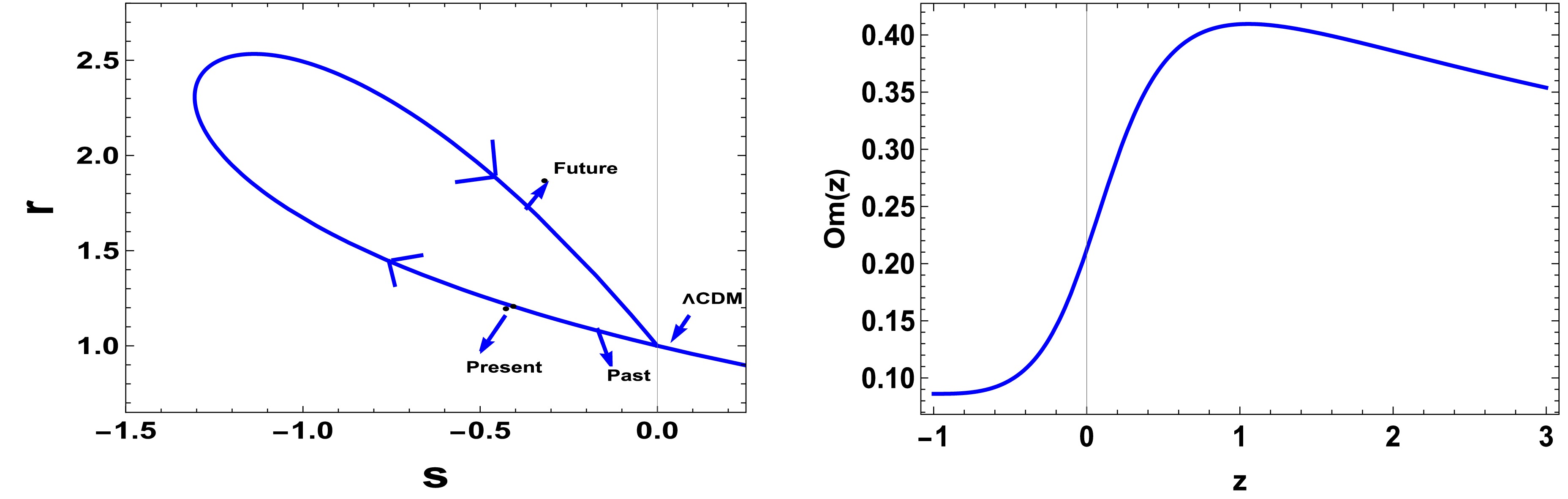
Figure 6. (color online) To check the models, we use two popular null tests for the ΛCDM model. First, we construct the
$ r-s $ plot, which shows late-time convergence to the ΛCDM model. We also use Om diagnostics to test the variation from ΛCDM for the Chaplygin gas model (as dark energy$ m\approx-5 $ ).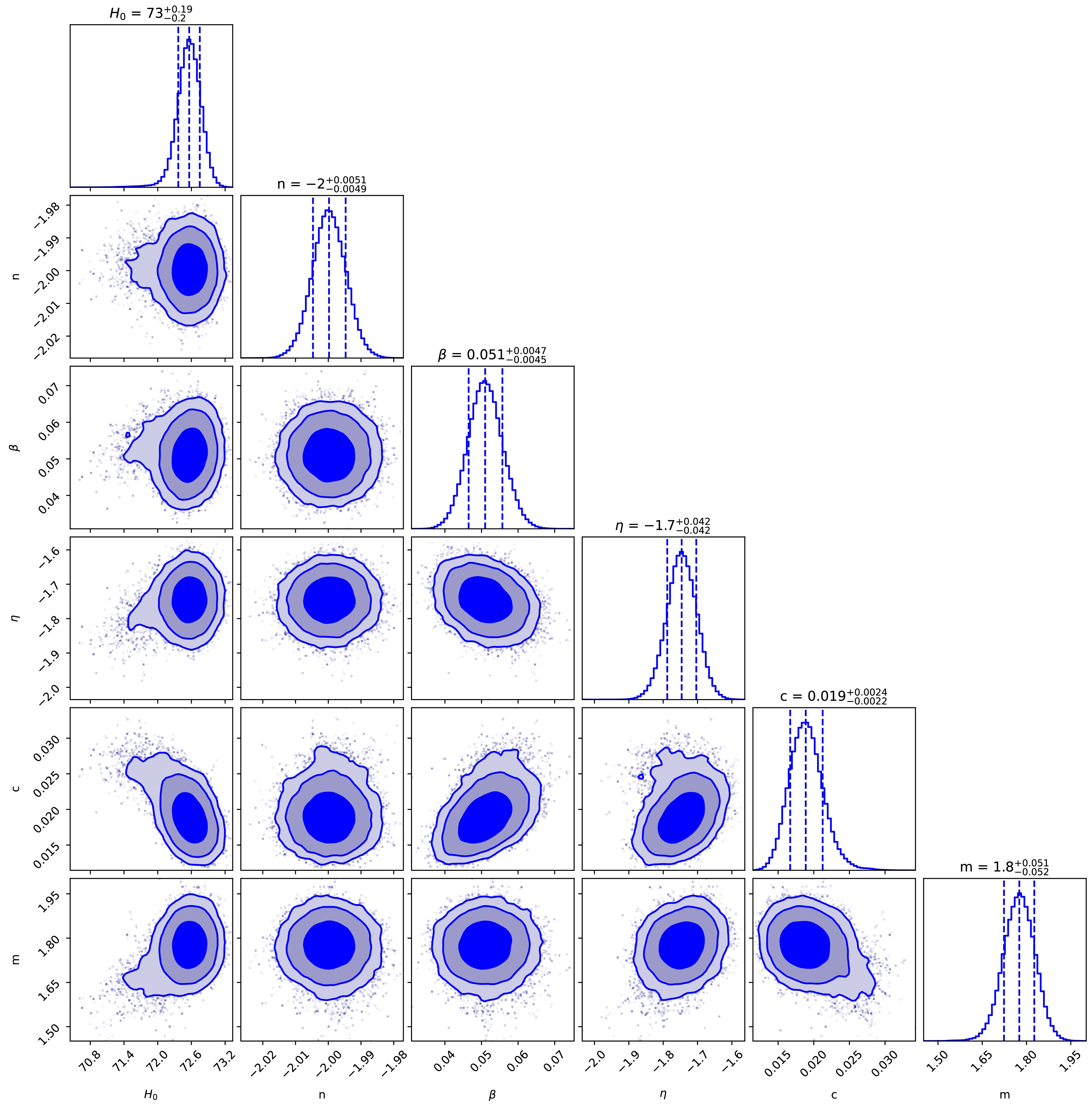
Figure 4. (color online) MCMC analysis for the Chaplygin gas model (as BEC dark matter
$ m\approx2 $ ). Based on a combined examination of the CC, BAO, and Pantheon+SH0ES datasets, the 2D-contour plot of the model parameters m, c, η,β, n, and$ H_0 $ displays the most likely values and confidence areas up to 3−σ.In general, both models indicate that they are globally in the phantom region.
-
Om diagnostics is the simplest form of diagnosis available for classification of the various dark energy-based cosmological models and their deviation from the ΛCDM.
It was first proposed by V. Sahni et al.[81], noting that the matter density falls as a third power of the scalar factor while the Λ remains constant. The formula for
$ Om(z) $ is given as,$ \begin{aligned} Om(z)=\frac{\left(\frac{H(z)}{H_0}\right)^2-1}{(1+z)^3-1} \end{aligned} $
(68) In our work, we have plotted this in the figure, and it shows that for approximately
$ z>1 $ the slope is negative, indicating quintessence scenarios, but for$ -1<z<1 $ the slope is positive, giving the phantom scenario. So, we can say for both of our cases that is both for the Chaplygin gas ($ m\approx -5 $ ) (Figure-6) and the BEC (Figure-$ m\approx 2 $ ) (Figure-4), we first obtain the quintessence scenario up to$ z=1, $ then from$ z=1 $ to present ($ z=0 $ ) and future ($ z<0 $ ) it follows phantom behavior to reach the de Sitter solution or ΛCDM. Therefore, both of our models exhibit phantom-like behavior in late times. This is not a contradiction, as the Om is susceptible to the full integration rather than the local instantaneous ω, so in a sense it measures the global evolution history of the$ H(z) $ , so in a sense we can say only after Om diagnosis that our model behavior is indeed phantom.
Figure 6. (color online) To check the models, we have used two very popular null tests for the ΛCDM model. First, we have done the
$ r-s $ plot, which shows that at late time it is converging to ΛCDM model, and we have also used Om diagnostics for testing variation from ΛCDM for the Chaplygin gas model (as dark energy$ m\approx-5 $ ).
Figure 4. (color online) The MCMC analysis for the Chaplygin gas model (as BEC dark matter
$ m\approx2 $ ). Based on a combined examination of the CC, BAO, and Pantheon+SH0ES datasets, the 2D-contour plot of the model parameters m, c, η,β, n, and$ H_0 $ displays the most likely values and the confidence areas up to 3−σ.So, in general, both models show that globally there are in the Phantom region.
-
Om diagnostics is the simplest form of diagnosis available for the classification of various dark energy-based cosmological models and their deviation from ΛCDM.
It was first proposed by Sahni et al. [81], who noted that the matter density falls as a third power of the scalar factor while Λ remains constant. The formula for
$ Om(z) $ is given as$ \begin{aligned} Om(z)=\frac{\left(\frac{H(z)}{H_0}\right)^2-1}{(1+z)^3-1}. \end{aligned} $
(72) In our study, we plot this relationship and find that, for approximately
$ z>1 $ , the slope is negative, indicating the quintessence scenario, whereas for$ -1<z<1 $ , the slope is positive, indicating the phantom scenario. Therefore, for both of our cases (the Chaplygin gas ($ m\approx -5 $ ) (Fig. 6) and BEC ($ m\approx 2 $ ) (Fig. 4)), the quintessence scenario is observed up to$ z=1, $ and then, from$ z=1 $ to the present ($ z=0 $ ) and future ($ z<0 $ ), the phantom behavior occurs to reach the de Sitter solution or ΛCDM. Therefore, both of our models exhibit late-time phantom-like behavior. This is not a contradiction, as the Om is susceptible to full integration rather than the local instantaneous ω. In a sense, it measures the global evolution history of$ H(z) $ ; hence, only after Om diagnosis can we suggest that our model behavior is indeed phantom.
Figure 6. (color online) To check the models, we use two popular null tests for the ΛCDM model. First, we construct the
$ r-s $ plot, which shows late-time convergence to the ΛCDM model. We also use Om diagnostics to test the variation from ΛCDM for the Chaplygin gas model (as dark energy$ m\approx-5 $ ).
Figure 4. (color online) MCMC analysis for the Chaplygin gas model (as BEC dark matter
$ m\approx2 $ ). Based on a combined examination of the CC, BAO, and Pantheon+SH0ES datasets, the 2D-contour plot of the model parameters m, c, η,β, n, and$ H_0 $ displays the most likely values and confidence areas up to 3−σ.In general, both models indicate that they are globally in the phantom region.
-
Om diagnostics is the simplest form of diagnosis available for the classification of various dark energy-based cosmological models and their deviation from ΛCDM.
It was first proposed by Sahni et al. [81], who noted that the matter density falls as a third power of the scalar factor while Λ remains constant. The formula for
$ Om(z) $ is given as$ \begin{aligned} Om(z)=\frac{\left(\frac{H(z)}{H_0}\right)^2-1}{(1+z)^3-1}. \end{aligned} $
(72) In our study, we plot this relationship and find that, for approximately
$ z>1 $ , the slope is negative, indicating the quintessence scenario, whereas for$ -1<z<1 $ , the slope is positive, indicating the phantom scenario. Therefore, for both of our cases (the Chaplygin gas ($ m\approx -5 $ ) and BEC ($ m\approx 2 $ ), the quintessence scenario is observed up to$ z=1, $ and then, from$ z=1 $ to the present ($ z=0 $ ) and future ($ z<0 $ ), the phantom behavior occurs to reach the de Sitter solution or ΛCDM. Therefore, both of our models exhibit late-time phantom-like behavior. This is not a contradiction, as the Om is susceptible to full integration rather than the local instantaneous ω. In a sense, it measures the global evolution history of$ H(z) $ ; hence, only after Om diagnosis can we suggest that our model behavior is indeed phantom.In general, both models indicate that they are globally in the phantom region.
-
Om diagnostics is the simplest form of diagnosis available for the classification of various dark energy-based cosmological models and their deviation from ΛCDM.
It was first proposed by Sahni et al. [81], who noted that the matter density falls as a third power of the scalar factor while Λ remains constant. The formula for
$ Om(z) $ is given as$ \begin{aligned} Om(z)=\frac{\left(\frac{H(z)}{H_0}\right)^2-1}{(1+z)^3-1}. \end{aligned} $
(72) In our study, we plot this relationship and find that, for approximately
$ z>1 $ , the slope is negative, indicating the quintessence scenario, whereas for$ -1<z<1 $ , the slope is positive, indicating the phantom scenario. Therefore, for both of our cases (the Chaplygin gas ($ m\approx -5 $ ) and BEC ($ m\approx 2 $ ), the quintessence scenario is observed up to$ z=1, $ and then, from$ z=1 $ to the present ($ z=0 $ ) and future ($ z<0 $ ), the phantom behavior occurs to reach the de Sitter solution or ΛCDM. Therefore, both of our models exhibit late-time phantom-like behavior. This is not a contradiction, as the Om is susceptible to full integration rather than the local instantaneous ω. In a sense, it measures the global evolution history of$ H(z) $ ; hence, only after Om diagnosis can we suggest that our model behavior is indeed phantom.In general, both models indicate that they are globally in the phantom region.
-
Om diagnostics is the simplest form of diagnosis available for the classification of various dark energy-based cosmological models and their deviation from ΛCDM.
It was first proposed by Sahni et al. [81], who noted that the matter density falls as a third power of the scalar factor while Λ remains constant. The formula for
$ Om(z) $ is given as$ \begin{aligned} Om(z)=\frac{\left(\frac{H(z)}{H_0}\right)^2-1}{(1+z)^3-1}. \end{aligned} $
(72) In our study, we plot this relationship and find that, for approximately
$ z>1 $ , the slope is negative, indicating the quintessence scenario, whereas for$ -1<z<1 $ , the slope is positive, indicating the phantom scenario. Therefore, for both of our cases (the Chaplygin gas ($ m\approx -5 $ ) and BEC ($ m\approx 2 $ ), the quintessence scenario is observed up to$ z=1, $ and then, from$ z=1 $ to the present ($ z=0 $ ) and future ($ z<0 $ ), the phantom behavior occurs to reach the de Sitter solution or ΛCDM. Therefore, both of our models exhibit late-time phantom-like behavior. This is not a contradiction, as the Om is susceptible to full integration rather than the local instantaneous ω. In a sense, it measures the global evolution history of$ H(z) $ ; hence, only after Om diagnosis can we suggest that our model behavior is indeed phantom.In general, both models indicate that they are globally in the phantom region.
-
Om diagnostics is the simplest form of diagnosis available for the classification of various dark energy-based cosmological models and their deviation from ΛCDM.
It was first proposed by Sahni et al. [81], who noted that the matter density falls as a third power of the scalar factor while Λ remains constant. The formula for
$ Om(z) $ is given as$ \begin{aligned} Om(z)=\frac{\left(\frac{H(z)}{H_0}\right)^2-1}{(1+z)^3-1}. \end{aligned} $
(72) In our study, we plot this relationship and find that, for approximately
$ z>1 $ , the slope is negative, indicating the quintessence scenario, whereas for$ -1<z<1 $ , the slope is positive, indicating the phantom scenario. Therefore, for both of our cases (the Chaplygin gas ($ m\approx -5 $ ) and BEC ($ m\approx 2 $ ), the quintessence scenario is observed up to$ z=1, $ and then, from$ z=1 $ to the present ($ z=0 $ ) and future ($ z<0 $ ), the phantom behavior occurs to reach the de Sitter solution or ΛCDM. Therefore, both of our models exhibit late-time phantom-like behavior. This is not a contradiction, as the Om is susceptible to full integration rather than the local instantaneous ω. In a sense, it measures the global evolution history of$ H(z) $ ; hence, only after Om diagnosis can we suggest that our model behavior is indeed phantom.In general, both models indicate that they are globally in the phantom region.
-
Om diagnostics is the simplest form of diagnosis available for the classification of various dark energy-based cosmological models and their deviation from ΛCDM.
It was first proposed by Sahni et al. [81], who noted that the matter density falls as a third power of the scalar factor while Λ remains constant. The formula for
$ Om(z) $ is given as$ \begin{aligned} Om(z)=\frac{\left(\frac{H(z)}{H_0}\right)^2-1}{(1+z)^3-1}. \end{aligned} $
(72) In our study, we plot this relationship and find that, for approximately
$ z>1 $ , the slope is negative, indicating the quintessence scenario, whereas for$ -1<z<1 $ , the slope is positive, indicating the phantom scenario. Therefore, for both of our cases (the Chaplygin gas ($ m\approx -5 $ ) and BEC ($ m\approx 2 $ ), the quintessence scenario is observed up to$ z=1, $ and then, from$ z=1 $ to the present ($ z=0 $ ) and future ($ z<0 $ ), the phantom behavior occurs to reach the de Sitter solution or ΛCDM. Therefore, both of our models exhibit late-time phantom-like behavior. This is not a contradiction, as the Om is susceptible to full integration rather than the local instantaneous ω. In a sense, it measures the global evolution history of$ H(z) $ ; hence, only after Om diagnosis can we suggest that our model behavior is indeed phantom.In general, both models indicate that they are globally in the phantom region.
-
Om diagnostics is the simplest form of diagnosis available for the classification of various dark energy-based cosmological models and their deviation from ΛCDM.
It was first proposed by Sahni et al. [81], who noted that the matter density falls as a third power of the scalar factor while Λ remains constant. The formula for
$ Om(z) $ is given as$ \begin{aligned} Om(z)=\frac{\left(\frac{H(z)}{H_0}\right)^2-1}{(1+z)^3-1}. \end{aligned} $
(72) In our study, we plot this relationship and find that, for approximately
$ z>1 $ , the slope is negative, indicating the quintessence scenario, whereas for$ -1<z<1 $ , the slope is positive, indicating the phantom scenario. Therefore, for both of our cases (the Chaplygin gas ($ m\approx -5 $ ) (Fig. 6) and BEC ($ m\approx 2 $ ) (Fig. 4)), the quintessence scenario is observed up to$ z=1, $ and then, from$ z=1 $ to the present ($ z=0 $ ) and future ($ z<0 $ ), the phantom behavior occurs to reach the de Sitter solution or ΛCDM. Therefore, both of our models exhibit late-time phantom-like behavior. This is not a contradiction, as the Om is susceptible to full integration rather than the local instantaneous ω. In a sense, it measures the global evolution history of$ H(z) $ ; hence, only after Om diagnosis can we suggest that our model behavior is indeed phantom.
Figure 6. (color online) To check the models, we use two popular null tests for the ΛCDM model. First, we construct the
$ r-s $ plot, which shows late-time convergence to the ΛCDM model. We also use Om diagnostics to test the variation from ΛCDM for the Chaplygin gas model (as dark energy$ m\approx-5 $ ).
Figure 4. (color online) MCMC analysis for the Chaplygin gas model (as BEC dark matter
$ m\approx2 $ ). Based on a combined examination of the CC, BAO, and Pantheon+SH0ES datasets, the 2D-contour plot of the model parameters m, c, η,β, n, and$ H_0 $ displays the most likely values and confidence areas up to 3−σ.In general, both models indicate that they are globally in the phantom region.
-
Although diagnosis Om is an excellent null test, there are several problems; for example, it does not distinguish between various types of quintessence and phantom models. There is also the fact that the formula is too simple, so it does not take into account the nuances of the other type of late cosmology and how much they differ from the ΛCDM.
In order to circumvent these things, V. Sahni et al. [82] have proposed a null test based on two different parameters that
$ r,s $ , where they are given by the formula:$ \begin{aligned} r=\frac{\dddot{a}}{aH^3} \end{aligned} $
(69) and
$ \begin{aligned} s=\frac{r-1}{3\left(q-\dfrac{1}{2}\right)} \end{aligned} $
(70) One first note is that for the standard ΛCDM model,
$ q=-1 $ , so$ r=0 $ , so one of the advantages of r is that even though many different models give similar H and q, they differ by the third derivative, that is, r. s is defined to distinguish between various forms of dark energy models. Together, r and s can distinguish between various models, such as Chaplygin gas, Phantom, Quintessence, etc. So, it can be easily shown that for ΛCDM ($ \omega=-1 $ )$ s=0,r=1 $ ; however,$ s<0 $ and$ r>1 $ (for both of our models), they are phantom in nature. However, it also shows that our current universe ($ z\approx 0 $ ) is located in the phantom region, and it will eventually converge to ΛCDM. It is worth noting that alone statefinder diagnosis alone can not tell any difference between Brane World or Chaplygin gas, we can not say for certainty which model of dark energy it represents, except the fact that it is not "pure quintessence" or a time-independent equation of state (i.e.$ \dot{\omega}\neq 0 $ ). It is worth noting that for a scalar field-based dark energy model, the statefinder, or more precisely s, does not uniquely specify the models. For example, a detailed analysis of the behavior with respect to the Phantom [83], interacting Phantom [84], and Quintom fields [85] reveals how the statefinder changes in general for all these potentials. -
Although Om diagnostics is an excellent null test, it has several problems; for example, it does not distinguish between various types of quintessence and phantom models. Moreover, the formula is too simple, so it does not take into account the nuances of the other types of late cosmology and how much they differ from ΛCDM.
To circumvent these issues, Sahni et al. [82] proposed a null test based on two different parameters,
$ r,s $ , given by the formulas$ \begin{aligned} r=\frac{\dddot{a}}{aH^3} \end{aligned} $
(73) and
$ \begin{aligned} s=\frac{r-1}{3\left(q-\dfrac{1}{2}\right)}. \end{aligned} $
(74) First, note that, for the standard ΛCDM model,
$ q=-1 $ ; hence,$ r=0 $ . Consequently, an advantage of r is that, although various models give similar H and q, they differ by the third derivative. In other words, r. s is defined to distinguish between various forms of dark energy models. Together, r and s can distinguish between various models, such as those of Chaplygin gas, phantom, and quintessence. Therefore, it can be easily shown that, for ΛCDM ($ \omega=-1 $ ),$ s=0,r=1 $ . However,$ s<0 $ and$ r>1 $ (for both of our models) are phantom in nature. This also shows that our current universe ($ z\approx 0 $ ) is located in the phantom region and will eventually converge to ΛCDM. It is worth noting that statefinder diagnosis alone cannot distinguish between brane world and Chaplygin gas, and we cannot say for certain which dark energy model is represented, except that it is neither "pure quintessence" nor a time-independent equation of state (i.e.,$ \dot{\omega}\neq 0 $ ). For a scalar field-based dark energy model, the statefinder, or more precisely s, does not uniquely specify the models. For example, a detailed analysis of the behavior with respect to the phantom [83], interacting phantom [84], and quintom fields [85] reveals how the statefinder generally changes for all these potentials. -
Although Om diagnostics is an excellent null test, it has several problems; for example, it does not distinguish between various types of quintessence and phantom models. Moreover, the formula is too simple, so it does not take into account the nuances of the other types of late cosmology and how much they differ from ΛCDM.
To circumvent these issues, Sahni et al. [82] proposed a null test based on two different parameters,
$ r,s $ , given by the formulas$ \begin{aligned} r=\frac{\dddot{a}}{aH^3} \end{aligned} $
(73) and
$ \begin{aligned} s=\frac{r-1}{3\left(q-\dfrac{1}{2}\right)}. \end{aligned} $
(74) First, note that, for the standard ΛCDM model,
$ q=-1 $ ; hence,$ r=0 $ . Consequently, an advantage of r is that, although various models give similar H and q, they differ by the third derivative. In other words, r. s is defined to distinguish between various forms of dark energy models. Together, r and s can distinguish between various models, such as those of Chaplygin gas, phantom, and quintessence. Therefore, it can be easily shown that, for ΛCDM ($ \omega=-1 $ ),$ s=0,r=1 $ . However,$ s<0 $ and$ r>1 $ (for both of our models) are phantom in nature. This also shows that our current universe ($ z\approx 0 $ ) is located in the phantom region and will eventually converge to ΛCDM. It is worth noting that statefinder diagnosis alone cannot distinguish between brane world and Chaplygin gas, and we cannot say for certain which dark energy model is represented, except that it is neither "pure quintessence" nor a time-independent equation of state (i.e.,$ \dot{\omega}\neq 0 $ ). For a scalar field-based dark energy model, the statefinder, or more precisely s, does not uniquely specify the models. For example, a detailed analysis of the behavior with respect to the phantom [83], interacting phantom [84], and quintom fields [85] reveals how the statefinder generally changes for all these potentials. -
Although Om diagnostics is an excellent null test, it has several problems; for example, it does not distinguish between various types of quintessence and phantom models. Moreover, the formula is too simple, so it does not take into account the nuances of the other types of late cosmology and how much they differ from ΛCDM.
To circumvent these issues, Sahni et al. [82] proposed a null test based on two different parameters,
$ r,s $ , given by the formulas$ \begin{aligned} r=\frac{\dddot{a}}{aH^3} \end{aligned} $
(73) and
$ \begin{aligned} s=\frac{r-1}{3\left(q-\dfrac{1}{2}\right)}. \end{aligned} $
(74) First, note that, for the standard ΛCDM model,
$ q=-1 $ ; hence,$ r=0 $ . Consequently, an advantage of r is that, although various models give similar H and q, they differ by the third derivative. In other words, r. s is defined to distinguish between various forms of dark energy models. Together, r and s can distinguish between various models, such as those of Chaplygin gas, phantom, and quintessence. Therefore, it can be easily shown that, for ΛCDM ($ \omega=-1 $ ),$ s=0,r=1 $ . However,$ s<0 $ and$ r>1 $ (for both of our models) are phantom in nature. This also shows that our current universe ($ z\approx 0 $ ) is located in the phantom region and will eventually converge to ΛCDM. It is worth noting that statefinder diagnosis alone cannot distinguish between brane world and Chaplygin gas, and we cannot say for certain which dark energy model is represented, except that it is neither "pure quintessence" nor a time-independent equation of state (i.e.,$ \dot{\omega}\neq 0 $ ). For a scalar field-based dark energy model, the statefinder, or more precisely s, does not uniquely specify the models. For example, a detailed analysis of the behavior with respect to the phantom [83], interacting phantom [84], and quintom fields [85] reveals how the statefinder generally changes for all these potentials. -
Although Om diagnostics is an excellent null test, it has several problems; for example, it does not distinguish between various types of quintessence and phantom models. Moreover, the formula is too simple, so it does not take into account the nuances of the other types of late cosmology and how much they differ from ΛCDM.
To circumvent these issues, Sahni et al. [82] proposed a null test based on two different parameters,
$ r,s $ , given by the formulas$ \begin{aligned} r=\frac{\dddot{a}}{aH^3} \end{aligned} $
(73) and
$ \begin{aligned} s=\frac{r-1}{3\left(q-\dfrac{1}{2}\right)}. \end{aligned} $
(74) First, note that, for the standard ΛCDM model,
$ q=-1 $ ; hence,$ r=0 $ . Consequently, an advantage of r is that, although various models give similar H and q, they differ by the third derivative. In other words, r. s is defined to distinguish between various forms of dark energy models. Together, r and s can distinguish between various models, such as those of Chaplygin gas, phantom, and quintessence. Therefore, it can be easily shown that, for ΛCDM ($ \omega=-1 $ ),$ s=0,r=1 $ . However,$ s<0 $ and$ r>1 $ (for both of our models) are phantom in nature. This also shows that our current universe ($ z\approx 0 $ ) is located in the phantom region and will eventually converge to ΛCDM. It is worth noting that statefinder diagnosis alone cannot distinguish between brane world and Chaplygin gas, and we cannot say for certain which dark energy model is represented, except that it is neither "pure quintessence" nor a time-independent equation of state (i.e.,$ \dot{\omega}\neq 0 $ ). For a scalar field-based dark energy model, the statefinder, or more precisely s, does not uniquely specify the models. For example, a detailed analysis of the behavior with respect to the phantom [83], interacting phantom [84], and quintom fields [85] reveals how the statefinder generally changes for all these potentials. -
Although Om diagnostics is an excellent null test, it has several problems; for example, it does not distinguish between various types of quintessence and phantom models. Moreover, the formula is too simple, so it does not take into account the nuances of the other types of late cosmology and how much they differ from ΛCDM.
To circumvent these issues, Sahni et al. [82] proposed a null test based on two different parameters,
$ r,s $ , given by the formulas$ \begin{aligned} r=\frac{\dddot{a}}{aH^3} \end{aligned} $
(73) and
$ \begin{aligned} s=\frac{r-1}{3\left(q-\dfrac{1}{2}\right)}. \end{aligned} $
(74) First, note that, for the standard ΛCDM model,
$ q=-1 $ ; hence,$ r=0 $ . Consequently, an advantage of r is that, although various models give similar H and q, they differ by the third derivative. In other words, r. s is defined to distinguish between various forms of dark energy models. Together, r and s can distinguish between various models, such as those of Chaplygin gas, phantom, and quintessence. Therefore, it can be easily shown that, for ΛCDM ($ \omega=-1 $ ),$ s=0,r=1 $ . However,$ s<0 $ and$ r>1 $ (for both of our models) are phantom in nature. This also shows that our current universe ($ z\approx 0 $ ) is located in the phantom region and will eventually converge to ΛCDM. It is worth noting that statefinder diagnosis alone cannot distinguish between brane world and Chaplygin gas, and we cannot say for certain which dark energy model is represented, except that it is neither "pure quintessence" nor a time-independent equation of state (i.e.,$ \dot{\omega}\neq 0 $ ). For a scalar field-based dark energy model, the statefinder, or more precisely s, does not uniquely specify the models. For example, a detailed analysis of the behavior with respect to the phantom [83], interacting phantom [84], and quintom fields [85] reveals how the statefinder generally changes for all these potentials. -
Although Om diagnostics is an excellent null test, it has several problems; for example, it does not distinguish between various types of quintessence and phantom models. Moreover, the formula is too simple, so it does not take into account the nuances of the other types of late cosmology and how much they differ from ΛCDM.
To circumvent these issues, Sahni et al. [82] proposed a null test based on two different parameters,
$ r,s $ , given by the formulas$ \begin{aligned} r=\frac{\dddot{a}}{aH^3} \end{aligned} $
(73) and
$ \begin{aligned} s=\frac{r-1}{3\left(q-\dfrac{1}{2}\right)}. \end{aligned} $
(74) First, note that, for the standard ΛCDM model,
$ q=-1 $ ; hence,$ r=0 $ . Consequently, an advantage of r is that, although various models give similar H and q, they differ by the third derivative. In other words, r. s is defined to distinguish between various forms of dark energy models. Together, r and s can distinguish between various models, such as those of Chaplygin gas, phantom, and quintessence. Therefore, it can be easily shown that, for ΛCDM ($ \omega=-1 $ ),$ s=0,r=1 $ . However,$ s<0 $ and$ r>1 $ (for both of our models) are phantom in nature. This also shows that our current universe ($ z\approx 0 $ ) is located in the phantom region and will eventually converge to ΛCDM. It is worth noting that statefinder diagnosis alone cannot distinguish between brane world and Chaplygin gas, and we cannot say for certain which dark energy model is represented, except that it is neither "pure quintessence" nor a time-independent equation of state (i.e.,$ \dot{\omega}\neq 0 $ ). For a scalar field-based dark energy model, the statefinder, or more precisely s, does not uniquely specify the models. For example, a detailed analysis of the behavior with respect to the phantom [83], interacting phantom [84], and quintom fields [85] reveals how the statefinder generally changes for all these potentials. -
Although Om diagnostics is an excellent null test, it has several problems; for example, it does not distinguish between various types of quintessence and phantom models. Moreover, the formula is too simple, so it does not take into account the nuances of the other types of late cosmology and how much they differ from ΛCDM.
To circumvent these issues, Sahni et al. [82] proposed a null test based on two different parameters,
$ r,s $ , given by the formulas$ \begin{aligned} r=\frac{\dddot{a}}{aH^3} \end{aligned} $
(73) and
$ \begin{aligned} s=\frac{r-1}{3\left(q-\dfrac{1}{2}\right)}. \end{aligned} $
(74) First, note that, for the standard ΛCDM model,
$ q=-1 $ ; hence,$ r=0 $ . Consequently, an advantage of r is that, although various models give similar H and q, they differ by the third derivative. In other words, r. s is defined to distinguish between various forms of dark energy models. Together, r and s can distinguish between various models, such as those of Chaplygin gas, phantom, and quintessence. Therefore, it can be easily shown that, for ΛCDM ($ \omega=-1 $ ),$ s=0,r=1 $ . However,$ s<0 $ and$ r>1 $ (for both of our models) are phantom in nature. This also shows that our current universe ($ z\approx 0 $ ) is located in the phantom region and will eventually converge to ΛCDM. It is worth noting that statefinder diagnosis alone cannot distinguish between brane world and Chaplygin gas, and we cannot say for certain which dark energy model is represented, except that it is neither "pure quintessence" nor a time-independent equation of state (i.e.,$ \dot{\omega}\neq 0 $ ). For a scalar field-based dark energy model, the statefinder, or more precisely s, does not uniquely specify the models. For example, a detailed analysis of the behavior with respect to the phantom [83], interacting phantom [84], and quintom fields [85] reveals how the statefinder generally changes for all these potentials. -
Although Om diagnostics is an excellent null test, it has several problems; for example, it does not distinguish between various types of quintessence and phantom models. Moreover, the formula is too simple, so it does not take into account the nuances of the other types of late cosmology and how much they differ from ΛCDM.
To circumvent these issues, Sahni et al. [82] proposed a null test based on two different parameters,
$ r,s $ , given by the formulas$ \begin{aligned} r=\frac{\dddot{a}}{aH^3} \end{aligned} $
(73) and
$ \begin{aligned} s=\frac{r-1}{3\left(q-\dfrac{1}{2}\right)}. \end{aligned} $
(74) First, note that, for the standard ΛCDM model,
$ q=-1 $ ; hence,$ r=0 $ . Consequently, an advantage of r is that, although various models give similar H and q, they differ by the third derivative. In other words, r. s is defined to distinguish between various forms of dark energy models. Together, r and s can distinguish between various models, such as those of Chaplygin gas, phantom, and quintessence. Therefore, it can be easily shown that, for ΛCDM ($ \omega=-1 $ ),$ s=0,r=1 $ . However,$ s<0 $ and$ r>1 $ (for both of our models) are phantom in nature. This also shows that our current universe ($ z\approx 0 $ ) is located in the phantom region and will eventually converge to ΛCDM. It is worth noting that statefinder diagnosis alone cannot distinguish between brane world and Chaplygin gas, and we cannot say for certain which dark energy model is represented, except that it is neither "pure quintessence" nor a time-independent equation of state (i.e.,$ \dot{\omega}\neq 0 $ ). For a scalar field-based dark energy model, the statefinder, or more precisely s, does not uniquely specify the models. For example, a detailed analysis of the behavior with respect to the phantom [83], interacting phantom [84], and quintom fields [85] reveals how the statefinder generally changes for all these potentials. -
Although Om diagnostics is an excellent null test, it has several problems; for example, it does not distinguish between various types of quintessence and phantom models. Moreover, the formula is too simple, so it does not take into account the nuances of the other types of late cosmology and how much they differ from ΛCDM.
To circumvent these issues, Sahni et al. [82] proposed a null test based on two different parameters,
$ r,s $ , given by the formulas$ \begin{aligned} r=\frac{\dddot{a}}{aH^3} \end{aligned} $
(73) and
$ \begin{aligned} s=\frac{r-1}{3\left(q-\dfrac{1}{2}\right)}. \end{aligned} $
(74) First, note that, for the standard ΛCDM model,
$ q=-1 $ ; hence,$ r=0 $ . Consequently, an advantage of r is that, although various models give similar H and q, they differ by the third derivative. In other words, r. s is defined to distinguish between various forms of dark energy models. Together, r and s can distinguish between various models, such as those of Chaplygin gas, phantom, and quintessence. Therefore, it can be easily shown that, for ΛCDM ($ \omega=-1 $ ),$ s=0,r=1 $ . However,$ s<0 $ and$ r>1 $ (for both of our models) are phantom in nature. This also shows that our current universe ($ z\approx 0 $ ) is located in the phantom region and will eventually converge to ΛCDM. It is worth noting that statefinder diagnosis alone cannot distinguish between brane world and Chaplygin gas, and we cannot say for certain which dark energy model is represented, except that it is neither "pure quintessence" nor a time-independent equation of state (i.e.,$ \dot{\omega}\neq 0 $ ). For a scalar field-based dark energy model, the statefinder, or more precisely s, does not uniquely specify the models. For example, a detailed analysis of the behavior with respect to the phantom [83], interacting phantom [84], and quintom fields [85] reveals how the statefinder generally changes for all these potentials. -
Although Om diagnostics is an excellent null test, it has several problems; for example, it does not distinguish between various types of quintessence and phantom models. Moreover, the formula is too simple, so it does not take into account the nuances of the other types of late cosmology and how much they differ from ΛCDM.
To circumvent these issues, Sahni et al. [82] proposed a null test based on two different parameters,
$ r,s $ , given by the formulas$ \begin{aligned} r=\frac{\dddot{a}}{aH^3} \end{aligned} $
(73) and
$ \begin{aligned} s=\frac{r-1}{3\left(q-\dfrac{1}{2}\right)}. \end{aligned} $
(74) First, note that, for the standard ΛCDM model,
$ q=-1 $ ; hence,$ r=0 $ . Consequently, an advantage of r is that, although various models give similar H and q, they differ by the third derivative. In other words, r. s is defined to distinguish between various forms of dark energy models. Together, r and s can distinguish between various models, such as those of Chaplygin gas, phantom, and quintessence. Therefore, it can be easily shown that, for ΛCDM ($ \omega=-1 $ ),$ s=0,r=1 $ . However,$ s<0 $ and$ r>1 $ (for both of our models) are phantom in nature. This also shows that our current universe ($ z\approx 0 $ ) is located in the phantom region and will eventually converge to ΛCDM. It is worth noting that statefinder diagnosis alone cannot distinguish between brane world and Chaplygin gas, and we cannot say for certain which dark energy model is represented, except that it is neither "pure quintessence" nor a time-independent equation of state (i.e.,$ \dot{\omega}\neq 0 $ ). For a scalar field-based dark energy model, the statefinder, or more precisely s, does not uniquely specify the models. For example, a detailed analysis of the behavior with respect to the phantom [83], interacting phantom [84], and quintom fields [85] reveals how the statefinder generally changes for all these potentials. -
In this study, we propose a unified model of dark energy and dark matter via the (generalized) Chaplygin gas model. We show that an MCMC analysis with both the Hubble and Pantheon+SH0ES datasets favors an MOG dark energy (
$ m\approx-5 $ ) and dark matter ($ m\approx=-2 $ ) dominated universe (dark energy originating from the MOG part). To systematically account for the transition, we employ a standard interaction term$ {\cal{I}} $ , which can serve as a mediator between dark matter and dark energy. Overall, we show that data analysis (ΔAIC and ΔBIC tests) favors the BEC dark-matter model over dark energy when using the pure Chaplygin gas model.Here is a brief overview of the final results presented in this manuscript. First, in Figs. 1 and 2, we present least squares fitting for the Hubble and supernova datasets and compare the Chaplygin gas (
$ m\approx-5 $ ) and BEC ($ m\approx2 $ ) models with the standard ΛCDM model to show the insignificant deviation between the two. This shows that, phenomenologically, our model is consistent with the current observation. Fig. 3 shows the results of the MCMC analysis; a$ 3\sigma $ contour plot is plotted using the corner plot in the EMCEE package in Python. Similarly, as shown in Fig. 4, we perform the same analysis for BEC dark matter and find that$ m\approx2 $ is also a valid solution, which produces a late-time de Sitter solution. Note that the obtained constraint$ n\neq1 $ does not contradict the standard GR tests, which allows for consistency between the MOG model and the data. Similar observations can be obtained in the context of$ f(R) $ gravity and also when adjusting it with large scale structures, X-rays [86], or UV-flux datasets [87]. This is analogous to the$ f(R) $ gravity case at lower scales, such as the Solar System or Shapiro time-delay-like experiments, where a screening mechanism adjusts the gravity to ensure it is consistent with the Einstein Hilbert action (as discussed in detail by Weltman et. al [88] and Harko et al. [89]). Fig. 5 shows the behaviors of phenomenological quantities such as q and$ \omega_{\rm eff} $ for$ m\approx-5 $ , followed by Fig. 6, which displays the statefinder and Om diagnostics for the same. Similarly, for$ m=2 $ , Figs. 7 and 8 present the phenomenological quantities and the null-test diagnostics, respectively. As expected, both cases exhibit late time de Sitter behavior (i.e., at$ z\rightarrow -1 $ ,$ q,\omega_{\rm eff}\rightarrow -1 $ ). The diagnostics indicate phantom behavior at current times and a late-time de Sitter transition, revealing the consistency of our model with the current paradigm.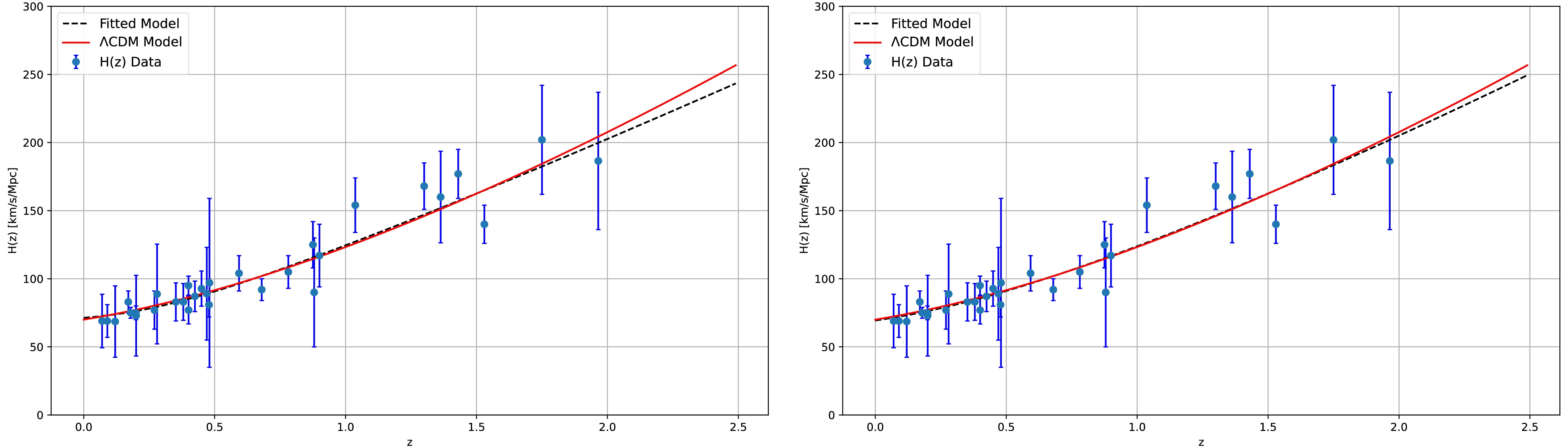
Figure 1. (color online) Least squares fitting for the Chaplygin gas model (left panel as dark energy
$ m\approx-5 $ and right panel as BEC dark matter$ m\approx2 $ ). The standard ΛCDM model (black dashed line) is compared with our proposed model fitted with the Hubble function$ H(z) $ versus redshift z (red line). An error bar plot representing the 31 CC dataset points considered for the analysis is also included.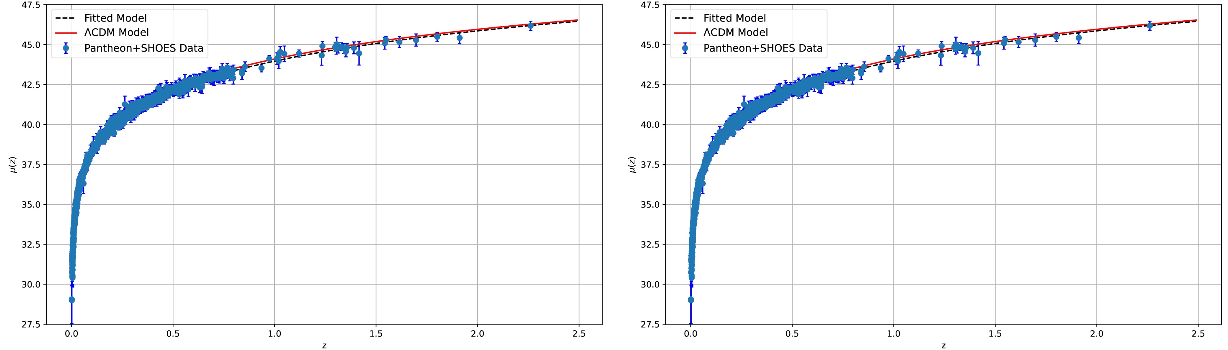
Figure 2. (color online) Least squares fitting for the Chaplygin gas model (left panel as dark energy
$ m\approx-5 $ and right panel as BEC dark matter$ m\approx2 $ ). The standard ΛCDM model (black dashed line) is compared with our proposed model fitted with the function$ \mu(z) $ versus redshift z (red line). An error bar plot representing the 1701 points of the Pantheon+SH0ES dataset considered for the analysis is also included.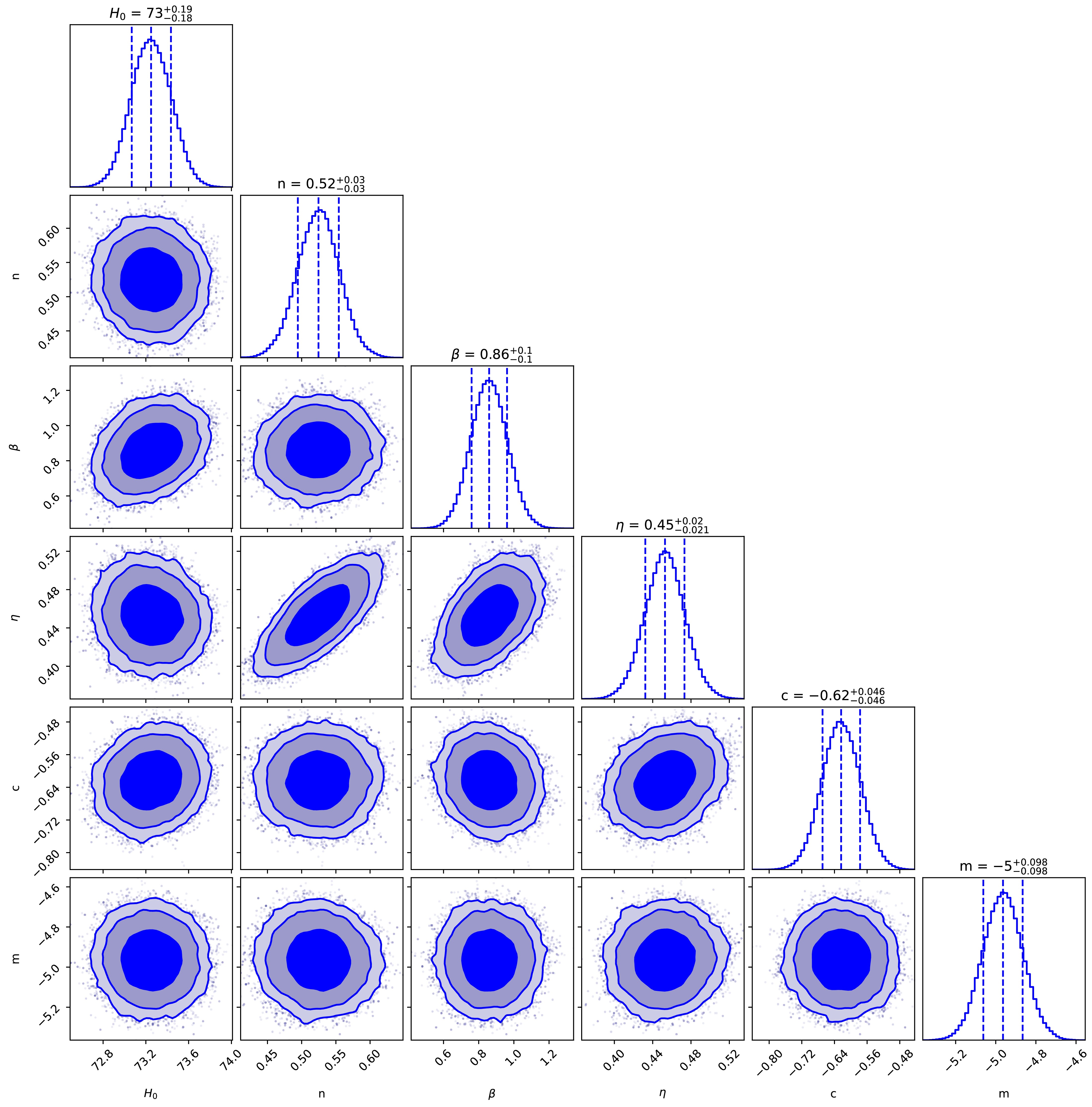
Figure 3. (color online) MCMC analysis for the Chaplygin gas model (as dark energy
$ m\approx-5 $ ). Based on a combined examination of the CC, BAO, and Pantheon+SH0ES datasets, the 2D-contour plot of the model parameters m, c, η, β, n, and$ H_0 $ displays the most likely values and confidence areas up to 3−σ.
Figure 4. (color online) MCMC analysis for the Chaplygin gas model (as BEC dark matter
$ m\approx2 $ ). Based on a combined examination of the CC, BAO, and Pantheon+SH0ES datasets, the 2D-contour plot of the model parameters m, c, η, β, n, and$ H_0 $ displays the most likely values and confidence areas up to 3−σ.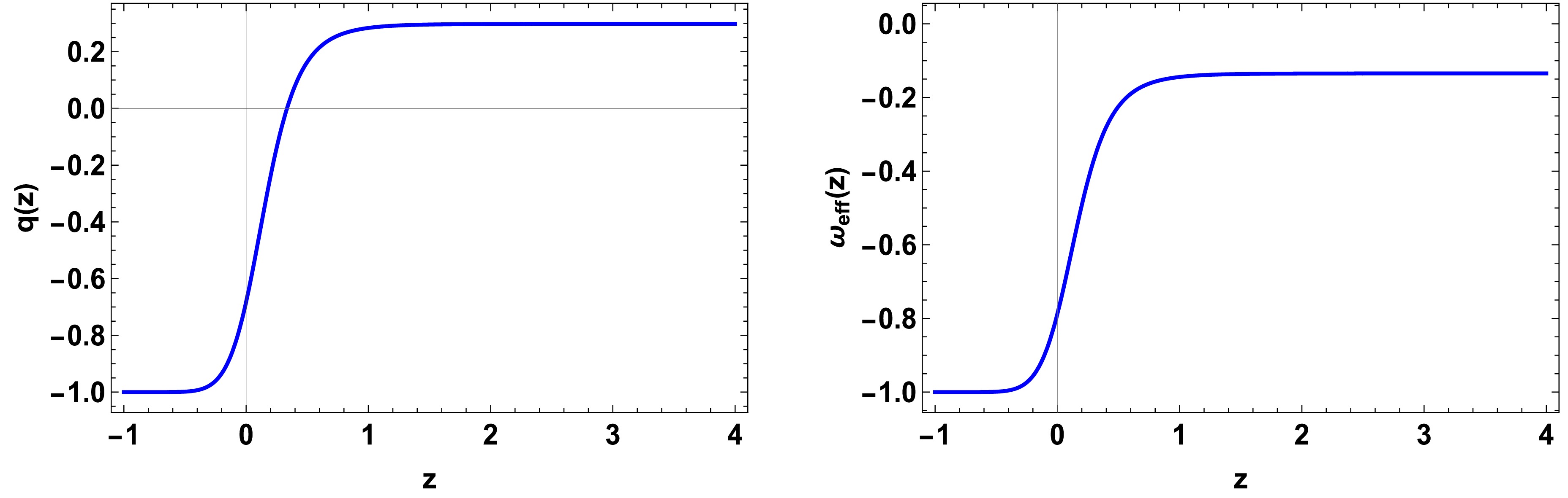
Figure 5. (color online) Deceleration parameter
$ q(z) $ and effective equations of state$ \omega(z) $ for the Chaplygin gas model (as dark energy$ m\approx-5 $ ). Both converge to −1 at$ z\xrightarrow{}-1 $ , as expected, which is highly consistent with the current values of the observed q and ω.
Figure 6. (color online) To check the models, we use two popular null tests for the ΛCDM model. First, we construct the
$ r-s $ plot, which shows late-time convergence to the ΛCDM model. We also use Om diagnostics to test the variation from ΛCDM for the Chaplygin gas model (as dark energy$ m\approx-5 $ ).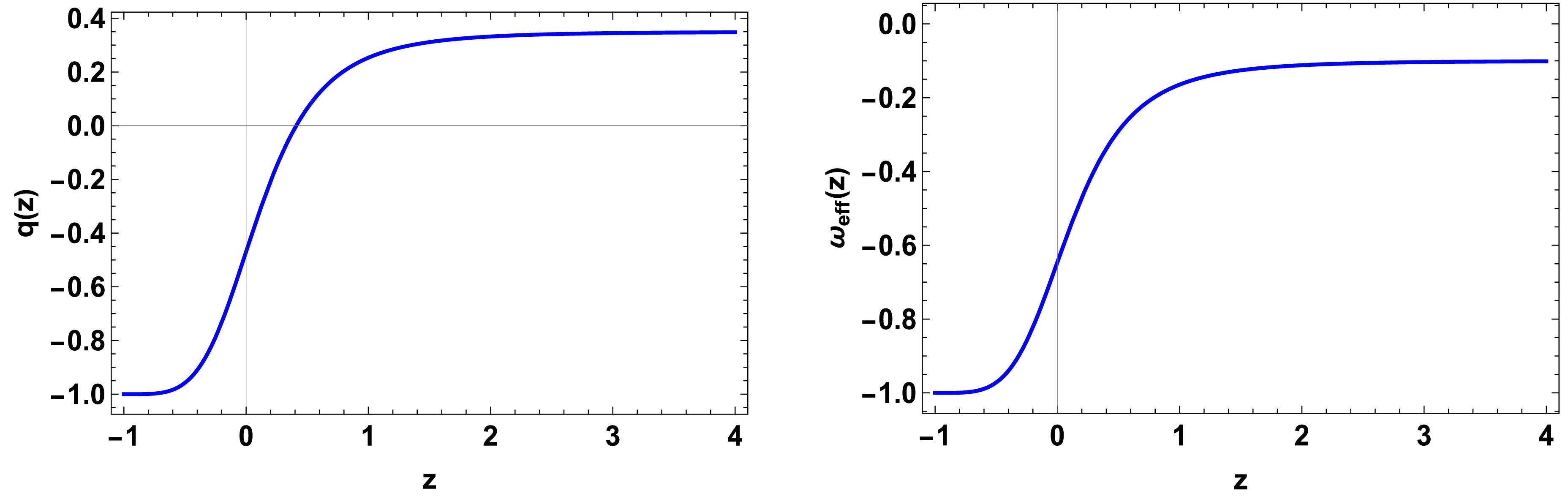
Figure 7. (color online) Deceleration parameter
$ q(z) $ and effective equations of state$ \omega(z) $ for the Chaplygin gas model (as dark matter$ m\approx2 $ ). Both converge to −1 at$ z\xrightarrow{}-1 $ , as expected, which is highly consistent with the current values of the observed q and ω.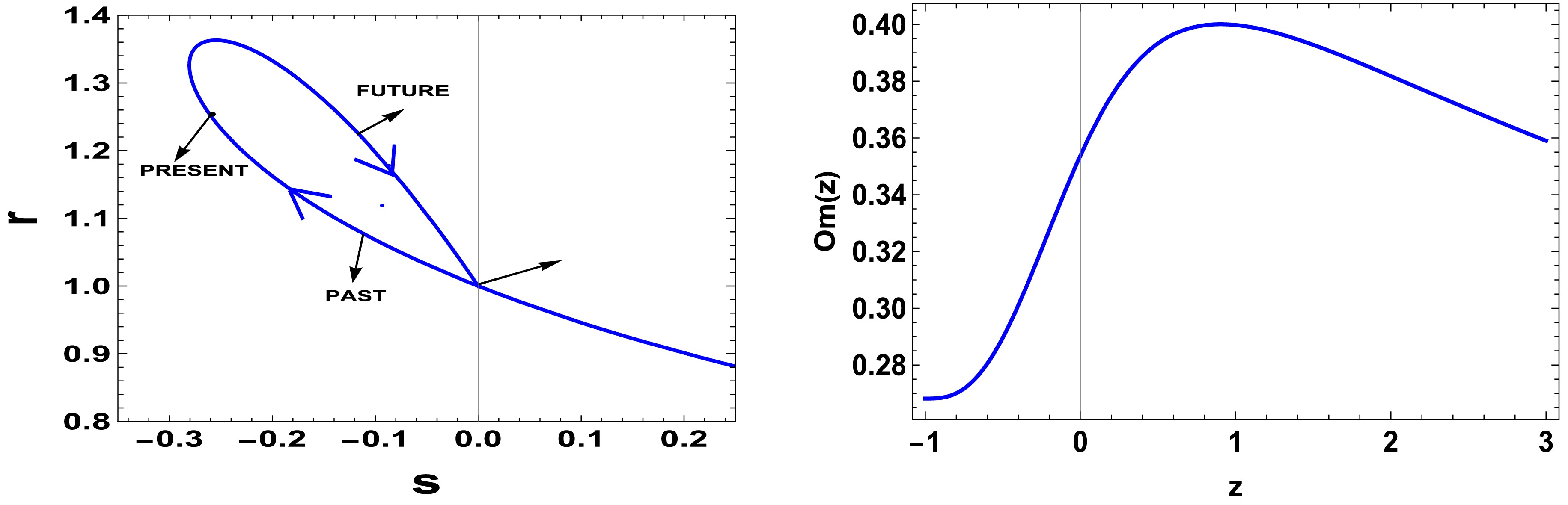
Figure 8. (color online) To check the models, we use two popular null tests for the ΛCDM model. First, we construct the
$ r-s $ plot, which shows late-time convergence to the ΛCDM model. We also use Om diagnostics to test the variation from ΛCDM for the Chaplygin gas model (as BEC dark matter$ m\approx2 $ ).Moreover, as listed in Table 3, after qualitatively examining ΔAIC and ΔBIC, our model is found to favor the BEC model over the Chaplygin gas model, confirming that there is a nontrivial interaction term between the two.
Here, we provide a brief outline of the entire paper.
First, we begin with the introduction (Section-I), where we detail our motivation for considering the Chaplygin gas equation of state as a unification of both dark matter and dark energy. We explain why Chaplygin gas models are appealing: they naturally occur in string theory and connect between a matter-dominated and dark-energy-dominated universe. We also discuss how the Bose-Einstein condensate could be a dark-matter candidate and the motivation for including the interaction term between dark matter and dark energy. After giving a brief outline of symmetric teleparallel-based gravity, we perform data analysis and null-tests (Om and statefinder diagnosis).
In Section II, we present a more detailed discussion on Chaplygin gas and show how various microscopic theories, such as the scalar field, DBI field, and brane world scenarios, can give rise to the Chaplygin gas equation of state. This section also serves as a primer indicating that the best fit for the Chaplygin gas model can be used to reconstruct the scalar field potential, DBI field potential, and even the wrapping factor for branes. Therefore, we demonstrate the universality of the Chaplygin gas model from both the microscopic and phenomenological perspectives.
In Section III, we discuss how dark matter can be modeled using BEC. We provide a brief physical motivation: the universe's state of formation could create an ideal environment for BEC to occur. BEC could explain the uniform density of dark-matter halos and is also an effective theory because, regardless the identity of the underlying bosons, if they are massive, there is a possibility for BEC. We also discuss the microscopic origin of BEC using the Gross-Pitaevskii equations for a weakly interacting Bose gas. Subsequently, we argue that the variation in such an energy function could lead to the Chaplygin gas equation-like form. Overall, this gives a microscopic and observationally sound reason for modeling dark matter as a Bose-Einstein condensate.
In Section IV, we advocate for a uniform framework for dark matter and dark energy, arguing that the values of m can be used to easily verify the domination of the model by dark energy, as described by the Chaplygin gas equation or BEC dark matter. We also discuss the need to include an interaction term to allow for consistency with the standard model of cosmology and to maintain the ratios of dark matter and dark energy.
In Section V, we give a brief description of
$ f(Q) $ gravity. We discuss the gauge choice and the reason why the boundary term does not impact the formulation. We then take a brief detour to explain a method of calculating the non-metric scalar from$ Q_{\alpha\mu\nu} $ . In Section VI, we continue the discussion on$ f(Q) $ gravity under the FLRW metric, taking a flat FLRW metric with signature (– + + +) and providing a way to calculate the non-metric scalar, which is found to be$ 6H^2 $ . We also argue that$ f(Q)=-Q $ can facilitate Einstein GR, providing a consistency check between MOG and standard Einstein GR.In Section VII, we provide the complete formula for
$ H(z) $ as a function of z (redshift), using the continuity equation and Friedmann equation to arrive at an exact formula. This enables us to perform data analysis and constrain the free parameters.In Section VIII, we perform a complete data analysis using the formula for
$ H(z) $ . We find two models: Model I ($ m\approx-5 $ ) and Model II ($ m\approx2 $ ), both of which yield constant observational values. Both models have similar q and ω, closely resembling our current universe's observational data. Although both models give observably constant results and satisfy the null tests, Model II, which is dark matter dominated, gives the lowest Δ AIC and Δ BIC, indicating that Chaplygin gas is more biased toward dark matter modeled by BEC. This also suggests that there is a non-trivial (as$ b\neq 0 $ ) interaction between dark matter and dark energy, that is, dark matter is transformed into dark energy.In Section IX, we perform two popular null tests for the ΛCDM model, namely, the Om and statefinder diagnoses. Both investigated models under the Om diagnosis approach the standard ΛCDM model while currently passing through the phantom epoch. In terms of the statefinder diagnosis, the results are also consistent with the phantom behavior; however, it could also denote any other form of the scalar fields, as mentioned above. This is unsurprising, as the Chaplygin gas equation of state typically gives phantom behavior. As shown in Section II, a non-standard kinetic energy term is required to arrive at the Chaplygin gas equation of state.
Finally, Section X presents the conclusion. Overall, this study demonstrates that a unified framework for dark matter and dark energy can be obtained through the Chaplygin gas model in
$ f(Q) $ MOG, and data analysis yields tight observational constraints on the free parameters. This study can be extended by using more general MOG models, such as$ f(Q,T),f(Q,B),f(Q,T) $ , or general$ f(Q,T,L_m) $ models, to ascertain whether the conclusions of our models are empirical. -
In this study, we propose a unified model of dark energy and dark matter via the (generalized) Chaplygin gas model. We show that an MCMC analysis with both the Hubble and Pantheon+SH0ES datasets favors an MOG dark energy (
$ m\approx-5 $ ) and dark matter ($ m\approx=-2 $ ) dominated universe (dark energy originating from the MOG part). To systematically account for the transition, we employ a standard interaction term$ {\cal{I}} $ , which can serve as a mediator between dark matter and dark energy. Overall, we show that data analysis (ΔAIC and ΔBIC tests) favors the BEC dark-matter model over dark energy when using the pure Chaplygin gas model.Here is a brief overview of the final results presented in this manuscript. First, in Figs. 1 and 2, we present least squares fitting for the Hubble and supernova datasets and compare the Chaplygin gas (
$ m\approx-5 $ ) and BEC ($ m\approx2 $ ) models with the standard ΛCDM model to show the insignificant deviation between the two. This shows that, phenomenologically, our model is consistent with the current observation. Fig. 3 shows the results of the MCMC analysis; a$ 3\sigma $ contour plot is plotted using the corner plot in the EMCEE package in Python. Similarly, as shown in Fig. 4, we perform the same analysis for BEC dark matter and find that$ m\approx2 $ is also a valid solution, which produces a late-time de Sitter solution. Note that the obtained constraint$ n\neq1 $ does not contradict the standard GR tests, which allows for consistency between the MOG model and the data. Similar observations can be obtained in the context of$ f(R) $ gravity and also when adjusting it with large scale structures, X-rays [86], or UV-flux datasets [87]. This is analogous to the$ f(R) $ gravity case at lower scales, such as the Solar System or Shapiro time-delay-like experiments, where a screening mechanism adjusts the gravity to ensure it is consistent with the Einstein Hilbert action (as discussed in detail by Weltman et. al [88] and Harko et al. [89]). Figs. 5 and 7 show the behaviors of phenomenological quantities such as q and$ \omega_{\rm eff} $ for$ m\approx-5 $ and$ m=2 $ , respectively. As expected, both exhibit late time de Sitter behavior (i.e., at$ z\rightarrow -1 $ ,$ q,\omega_{\rm eff}\rightarrow -1 $ ). Finally, Figs. 6 and 8 show the results of the two most famous null-tests for the ΛCDM model, that is, statefinder and Om diagnostics, both of which indicate phantom behavior in the current time and late-time de Sitter transition. This reveals the consistency of our model with the current paradigm.
Figure 1. (color online) Least squares fitting for the Chaplygin gas model (left panel as dark energy
$ m\approx-5 $ and right panel as BEC dark matter$ m\approx2 $ ). The standard ΛCDM model (black dashed line) is compared with our proposed model fitted with the Hubble function$ H(z) $ versus redshift z (red line). An error bar plot representing the 31 CC dataset points considered for the analysis is also included.
Figure 2. (color online) Least squares fitting for the Chaplygin gas model (left panel as dark energy
$ m\approx-5 $ and right panel as BEC dark matter$ m\approx2 $ ). The standard ΛCDM model (black dashed line) is compared with our proposed model fitted with the function$ \mu(z) $ versus redshift z (red line). An error bar plot representing the 1701 points of the Pantheon+SH0ES dataset considered for the analysis is also included.
Figure 3. (color online) MCMC analysis for the Chaplygin gas model (as dark energy
$ m\approx-5 $ ). Based on a combined examination of the CC, BAO, and Pantheon+SH0ES datasets, the 2D-contour plot of the model parameters m, c, η, β, n, and$ H_0 $ displays the most likely values and confidence areas up to 3−σ.
Figure 5. (color online) Deceleration parameter
$ q(z) $ and effective equations of state$ \omega(z) $ for the Chaplygin gas model (as dark energy$ m\approx-5 $ ). Both converge to −1 at$ z\xrightarrow{}-1 $ , as expected, which is highly consistent with the current values of the observed q and ω.
Figure 7. (color online) Deceleration parameter
$ q(z) $ and effective equations of state$ \omega(z) $ for the Chaplygin gas model (as dark matter$ m\approx2 $ ). Both converge to −1 at$ z\xrightarrow{}-1 $ , as expected, which is highly consistent with the current values of the observed q and ω.
Figure 8. (color online) To check the models, we use two popular null tests for the ΛCDM model. First, we construct the
$ r-s $ plot, which shows late-time convergence to the ΛCDM model. We also use Om diagnostics to test the variation from ΛCDM for the Chaplygin gas model (as BEC dark matter$ m\approx2 $ ).Moreover, as listed in Table 3, after qualitatively examining ΔAIC and ΔBIC, our model is found to favor the BEC model over the Chaplygin gas model, confirming that there is a nontrivial interaction term between the two.
Here, we provide a brief outline of the entire paper.
First, we begin with the introduction (Section-I), where we detail our motivation for considering the Chaplygin gas equation of state as a unification of both dark matter and dark energy. We explain why Chaplygin gas models are appealing: they naturally occur in string theory and connect between a matter-dominated and dark-energy-dominated universe. We also discuss how the Bose-Einstein condensate could be a dark-matter candidate and the motivation for including the interaction term between dark matter and dark energy. After giving a brief outline of symmetric teleparallel-based gravity, we perform data analysis and null-tests (Om and statefinder diagnosis).
In Section II, we present a more detailed discussion on Chaplygin gas and show how various microscopic theories, such as the scalar field, DBI field, and brane world scenarios, can give rise to the Chaplygin gas equation of state. This section also serves as a primer indicating that the best fit for the Chaplygin gas model can be used to reconstruct the scalar field potential, DBI field potential, and even the wrapping factor for branes. Therefore, we demonstrate the universality of the Chaplygin gas model from both the microscopic and phenomenological perspectives.
In Section III, we discuss how dark matter can be modeled using BEC. We provide a brief physical motivation: the universe's state of formation could create an ideal environment for BEC to occur. BEC could explain the uniform density of dark-matter halos and is also an effective theory because, regardless the identity of the underlying bosons, if they are massive, there is a possibility for BEC. We also discuss the microscopic origin of BEC using the Gross-Pitaevskii equations for a weakly interacting Bose gas. Subsequently, we argue that the variation in such an energy function could lead to the Chaplygin gas equation-like form. Overall, this gives a microscopic and observationally sound reason for modeling dark matter as a Bose-Einstein condensate.
In Section IV, we advocate for a uniform framework for dark matter and dark energy, arguing that the values of m can be used to easily verify the domination of the model by dark energy, as described by the Chaplygin gas equation or BEC dark matter. We also discuss the need to include an interaction term to allow for consistency with the standard model of cosmology and to maintain the ratios of dark matter and dark energy.
In Section V, we give a brief description of
$ f(Q) $ gravity. We discuss the gauge choice and the reason why the boundary term does not impact the formulation. We then take a brief detour to explain a method of calculating the non-metric scalar from$ Q_{\alpha\mu\nu} $ . In Section VI, we continue the discussion on$ f(Q) $ gravity under the FLRW metric, taking a flat FLRW metric with signature (– + + +) and providing a way to calculate the non-metric scalar, which is found to be$ 6H^2 $ . We also argue that$ f(Q)=-Q $ can facilitate Einstein GR, providing a consistency check between MOG and standard Einstein GR.In Section VII, we provide the complete formula for
$ H(z) $ as a function of z (redshift), using the continuity equation and Friedmann equation to arrive at an exact formula. This enables us to perform data analysis and constrain the free parameters.In Section VIII, we perform a complete data analysis using the formula for
$ H(z) $ . We find two models: Model I ($ m\approx-5 $ ) and Model II ($ m\approx2 $ ), both of which yield constant observational values. Both models have similar q and ω, closely resembling our current universe's observational data. Although both models give observably constant results and satisfy the null tests, Model II, which is dark matter dominated, gives the lowest Δ AIC and Δ BIC, indicating that Chaplygin gas is more biased toward dark matter modeled by BEC. This also suggests that there is a non-trivial (as$ b\neq 0 $ ) interaction between dark matter and dark energy, that is, dark matter is transformed into dark energy.In Section IX, we perform two popular null tests for the ΛCDM model, namely, the Om and statefinder diagnoses. Both investigated models under the Om diagnosis approach the standard ΛCDM model while currently passing through the phantom epoch. In terms of the statefinder diagnosis, the results are also consistent with the phantom behavior; however, it could also denote any other form of the scalar fields, as mentioned above. This is unsurprising, as the Chaplygin gas equation of state typically gives phantom behavior. As shown in Section II, a non-standard kinetic energy term is required to arrive at the Chaplygin gas equation of state.
Finally, Section X presents the conclusion. Overall, this study demonstrates that a unified framework for dark matter and dark energy can be obtained through the Chaplygin gas model in
$ f(Q) $ MOG, and data analysis yields tight observational constraints on the free parameters. This study can be extended by using more general MOG models, such as$ f(Q,T),f(Q,B),f(Q,T) $ , or general$ f(Q,T,L_m) $ models, to ascertain whether the conclusions of our models are empirical. -
In this study, we propose a unified model of dark energy and dark matter via the (generalized) Chaplygin gas model. We show that an MCMC analysis with both the Hubble and Pantheon+SH0ES datasets favors an MOG dark energy (
$ m\approx-5 $ ) and dark matter ($ m\approx=-2 $ ) dominated universe (dark energy originating from the MOG part). To systematically account for the transition, we employ a standard interaction term$ {\cal{I}} $ , which can serve as a mediator between dark matter and dark energy. Overall, we show that data analysis (ΔAIC and ΔBIC tests) favors the BEC dark-matter model over dark energy when using the pure Chaplygin gas model.Here is a brief overview of the final results presented in this manuscript. First, in Figs. 1 and 2, we present least squares fitting for the Hubble and supernova datasets and compare the Chaplygin gas (
$ m\approx-5 $ ) and BEC ($ m\approx2 $ ) models with the standard ΛCDM model to show the insignificant deviation between the two. This shows that, phenomenologically, our model is consistent with the current observation. Fig. 3 shows the results of the MCMC analysis; a$ 3\sigma $ contour plot is plotted using the corner plot in the EMCEE package in Python. Similarly, as shown in Fig. 4, we perform the same analysis for BEC dark matter and find that$ m\approx2 $ is also a valid solution, which produces a late-time de Sitter solution. Note that the obtained constraint$ n\neq1 $ does not contradict the standard GR tests, which allows for consistency between the MOG model and the data. Similar observations can be obtained in the context of$ f(R) $ gravity and also when adjusting it with large scale structures, X-rays [86], or UV-flux datasets [87]. This is analogous to the$ f(R) $ gravity case at lower scales, such as the Solar System or Shapiro time-delay-like experiments, where a screening mechanism adjusts the gravity to ensure it is consistent with the Einstein Hilbert action (as discussed in detail by Weltman et. al [88] and Harko et al. [89]). Fig. 5 shows the behaviors of phenomenological quantities such as q and$ \omega_{\rm eff} $ for$ m\approx-5 $ , followed by Fig. 6, which displays the statefinder and Om diagnostics for the same. Similarly, for$ m=2 $ , Figs. 7 and 8 present the phenomenological quantities and the null-test diagnostics, respectively. As expected, both cases exhibit late time de Sitter behavior (i.e., at$ z\rightarrow -1 $ ,$ q,\omega_{\rm eff}\rightarrow -1 $ ). The diagnostics indicate phantom behavior at current times and a late-time de Sitter transition, revealing the consistency of our model with the current paradigm.
Figure 1. (color online) Least squares fitting for the Chaplygin gas model (left panel as dark energy
$ m\approx-5 $ and right panel as BEC dark matter$ m\approx2 $ ). The standard ΛCDM model (black dashed line) is compared with our proposed model fitted with the Hubble function$ H(z) $ versus redshift z (red line). An error bar plot representing the 31 CC dataset points considered for the analysis is also included.
Figure 2. (color online) Least squares fitting for the Chaplygin gas model (left panel as dark energy
$ m\approx-5 $ and right panel as BEC dark matter$ m\approx2 $ ). The standard ΛCDM model (black dashed line) is compared with our proposed model fitted with the function$ \mu(z) $ versus redshift z (red line). An error bar plot representing the 1701 points of the Pantheon+SH0ES dataset considered for the analysis is also included.
Figure 3. (color online) MCMC analysis for the Chaplygin gas model (as dark energy
$ m\approx-5 $ ). Based on a combined examination of the CC, BAO, and Pantheon+SH0ES datasets, the 2D-contour plot of the model parameters m, c, η, β, n, and$ H_0 $ displays the most likely values and confidence areas up to 3−σ.
Figure 4. (color online) MCMC analysis for the Chaplygin gas model (as BEC dark matter
$ m\approx2 $ ). Based on a combined examination of the CC, BAO, and Pantheon+SH0ES datasets, the 2D-contour plot of the model parameters m, c, η, β, n, and$ H_0 $ displays the most likely values and confidence areas up to 3−σ.
Figure 5. (color online) Deceleration parameter
$ q(z) $ and effective equations of state$ \omega(z) $ for the Chaplygin gas model (as dark energy$ m\approx-5 $ ). Both converge to −1 at$ z\xrightarrow{}-1 $ , as expected, which is highly consistent with the current values of the observed q and ω.
Figure 6. (color online) To check the models, we use two popular null tests for the ΛCDM model. First, we construct the
$ r-s $ plot, which shows late-time convergence to the ΛCDM model. We also use Om diagnostics to test the variation from ΛCDM for the Chaplygin gas model (as dark energy$ m\approx-5 $ ).
Figure 7. (color online) Deceleration parameter
$ q(z) $ and effective equations of state$ \omega(z) $ for the Chaplygin gas model (as dark matter$ m\approx2 $ ). Both converge to −1 at$ z\xrightarrow{}-1 $ , as expected, which is highly consistent with the current values of the observed q and ω.
Figure 8. (color online) To check the models, we use two popular null tests for the ΛCDM model. First, we construct the
$ r-s $ plot, which shows late-time convergence to the ΛCDM model. We also use Om diagnostics to test the variation from ΛCDM for the Chaplygin gas model (as BEC dark matter$ m\approx2 $ ).Moreover, as listed in Table 3, after qualitatively examining ΔAIC and ΔBIC, our model is found to favor the BEC model over the Chaplygin gas model, confirming that there is a nontrivial interaction term between the two.
Here, we provide a brief outline of the entire paper.
First, we begin with the introduction (Section-I), where we detail our motivation for considering the Chaplygin gas equation of state as a unification of both dark matter and dark energy. We explain why Chaplygin gas models are appealing: they naturally occur in string theory and connect between a matter-dominated and dark-energy-dominated universe. We also discuss how the Bose-Einstein condensate could be a dark-matter candidate and the motivation for including the interaction term between dark matter and dark energy. After giving a brief outline of symmetric teleparallel-based gravity, we perform data analysis and null-tests (Om and statefinder diagnosis).
In Section II, we present a more detailed discussion on Chaplygin gas and show how various microscopic theories, such as the scalar field, DBI field, and brane world scenarios, can give rise to the Chaplygin gas equation of state. This section also serves as a primer indicating that the best fit for the Chaplygin gas model can be used to reconstruct the scalar field potential, DBI field potential, and even the wrapping factor for branes. Therefore, we demonstrate the universality of the Chaplygin gas model from both the microscopic and phenomenological perspectives.
In Section III, we discuss how dark matter can be modeled using BEC. We provide a brief physical motivation: the universe's state of formation could create an ideal environment for BEC to occur. BEC could explain the uniform density of dark-matter halos and is also an effective theory because, regardless the identity of the underlying bosons, if they are massive, there is a possibility for BEC. We also discuss the microscopic origin of BEC using the Gross-Pitaevskii equations for a weakly interacting Bose gas. Subsequently, we argue that the variation in such an energy function could lead to the Chaplygin gas equation-like form. Overall, this gives a microscopic and observationally sound reason for modeling dark matter as a Bose-Einstein condensate.
In Section IV, we advocate for a uniform framework for dark matter and dark energy, arguing that the values of m can be used to easily verify the domination of the model by dark energy, as described by the Chaplygin gas equation or BEC dark matter. We also discuss the need to include an interaction term to allow for consistency with the standard model of cosmology and to maintain the ratios of dark matter and dark energy.
In Section V, we give a brief description of
$ f(Q) $ gravity. We discuss the gauge choice and the reason why the boundary term does not impact the formulation. We then take a brief detour to explain a method of calculating the non-metric scalar from$ Q_{\alpha\mu\nu} $ . In Section VI, we continue the discussion on$ f(Q) $ gravity under the FLRW metric, taking a flat FLRW metric with signature (– + + +) and providing a way to calculate the non-metric scalar, which is found to be$ 6H^2 $ . We also argue that$ f(Q)=-Q $ can facilitate Einstein GR, providing a consistency check between MOG and standard Einstein GR.In Section VII, we provide the complete formula for
$ H(z) $ as a function of z (redshift), using the continuity equation and Friedmann equation to arrive at an exact formula. This enables us to perform data analysis and constrain the free parameters.In Section VIII, we perform a complete data analysis using the formula for
$ H(z) $ . We find two models: Model I ($ m\approx-5 $ ) and Model II ($ m\approx2 $ ), both of which yield constant observational values. Both models have similar q and ω, closely resembling our current universe's observational data. Although both models give observably constant results and satisfy the null tests, Model II, which is dark matter dominated, gives the lowest Δ AIC and Δ BIC, indicating that Chaplygin gas is more biased toward dark matter modeled by BEC. This also suggests that there is a non-trivial (as$ b\neq 0 $ ) interaction between dark matter and dark energy, that is, dark matter is transformed into dark energy.In Section IX, we perform two popular null tests for the ΛCDM model, namely, the Om and statefinder diagnoses. Both investigated models under the Om diagnosis approach the standard ΛCDM model while currently passing through the phantom epoch. In terms of the statefinder diagnosis, the results are also consistent with the phantom behavior; however, it could also denote any other form of the scalar fields, as mentioned above. This is unsurprising, as the Chaplygin gas equation of state typically gives phantom behavior. As shown in Section II, a non-standard kinetic energy term is required to arrive at the Chaplygin gas equation of state.
Finally, Section X presents the conclusion. Overall, this study demonstrates that a unified framework for dark matter and dark energy can be obtained through the Chaplygin gas model in
$ f(Q) $ MOG, and data analysis yields tight observational constraints on the free parameters. This study can be extended by using more general MOG models, such as$ f(Q,T),f(Q,B),f(Q,T) $ , or general$ f(Q,T,L_m) $ models, to ascertain whether the conclusions of our models are empirical. -
In this article, we have offered a unified model of both dark energy and dark matter via the (Generalized) Chaplygin Gas model. We have shown that the MCMC analysis with both Hubble and Pantheon+SH0ES data sets favors the modified gravity dark energy (
$ m\approx-5 $ ) as well as dark matter ($ m\approx=-2 $ ) dominated universe (dark energy coming from the modified gravity part). To systematically account for the transition, we have employed a standard interaction term$ {\cal{I}} $ , which can serve as a mediator between dark matter and dark energy. Overall, we have shown that data analysis (ΔAIC and ΔBIC tests) favors the BEC dark-matter model over dark energy purely by the Chaplygin gas model.Here is a brief overview of the final results, which are presented throughout the manuscript. First of all, in the Fig. 1 and Fig. 2, we have given the least square fitting for the Hubble and SN data set and compared our model Chaplygin Gas (
$ m\approx-5 $ ) and BEC ($ m\approx2 $ ) respectively, with the standard ΛCDM model to show that there is not much significant deviation between the two, which shows that at least phenomenologically, our model is consistent with the current observation. For Fig. 3, we have done the MCMC analysis and plotted the$ 3\sigma $ contour plot using the corner plot in the EMCEE package in Python. Similarly, in Fig. 4, we have performed the same analysis for BEC dark matter and shown that indeed$ m\approx2 $ is also a valid solution, which produces a late-time de Sitter solution. Also note that the obtained constraint$ n\neq1 $ does not contradict the standard GR tests, in a sense this gives the freedom to modified gravity model to be consistent with the data, very similar things can be seen in the context of$ f(R) $ gravity, and also when one try to adjust it with large scale structure or X-ray [86] or UV-flux datasets [87]. It is analogous to$ f(R) $ gravity case in lower scales such as the solar system or Shapiro time-delay-like experiments, there always exists a screening mechanism to adjust the gravity to make sure it is consistent with the Einstein Hilbert action, which is discussed in detail by Weltman et. al [88] and Harko et. al. [89]. In Fig. 5 and Fig. 7, we have shown the behaviors for the phenomenological quantities such as q and$ \omega_{eff} $ for both$ m\approx-5 $ and$ m=2 $ , respectively. As expected, both of them are showing late time de Sitter behavior (i.e., at$ z\rightarrow -1 $ ,$ q,\omega_{eff}\rightarrow -1 $ ). Finally, in Fig. 6 and Fig. 8 we have done the two most famous Null-tests for the ΛCDM model, that is, the statefinder and Om diagnostics, both of which show the Phantom behavior in the current time and late-time de Sitter transition, showing the consistency of our model with the current paradigm.
Figure 1. (color online) The least square fitting for the Chaplygin gas model (left panel as dark energy
$ m\approx-5 $ and right panel as BEC dark matter$ m\approx2 $ ). In comparison to the standard ΛCDM model (black dashed line), the figure displays the fitting of the Hubble function$ H(z) $ versus redshift z for our proposed model (red line). An error bar plot representing the 31 CC dataset points considered for the analysis is also included.
Figure 2. (color online) The least square fitting for the Chaplygin gas model (left panel as dark energy
$ m\approx-5 $ and right panel as BEC dark matter$ m\approx2 $ ). In comparison to the standard ΛCDM model (black dashed line), the figure displays the fitting of the function$ \mu(z) $ versus redshift z for our proposed model (red line). An error bar plot representing the 1701 points of the Pantheon+SH0ES dataset considered for the analysis is also included.
Figure 3. (color online) The MCMC analysis for the Chaplygin gas model (as dark energy
$ m\approx-5 $ ). Based on a combined examination of the CC, BAO, and Pantheon+SH0ES datasets, the 2D-contour plot of the model parameters m, c, η,β, n, and$ H_0 $ displays the most likely values and the confidence areas up to 3−σ.
Figure 5. (color online) The deceleration parameter
$ q(z) $ and effective equations of state$ \omega(z) $ for the Chaplygin gas model (as dark energy$ m\approx-5 $ ). As both blots show at$ z\xrightarrow{}-1 $ , both of them converge to −1 as expected, and also it is very consistent with the current values of the observed q and ω
Figure 7. (color online) The deceleration parameter
$ q(z) $ and effective equations of state$ \omega(z) $ for the Chaplygin gas model (as dark matter$ m\approx2 $ ). As both blots show at$ z\xrightarrow{}-1 $ , both converge to −1 as expected, and it is also very consistent with the current values of the observed q and ω
Figure 8. (color online) To check the models, we have used two very popular null tests for the ΛCDM model. First, we have done the
$ r-s $ plot, which shows that at late time it is converging to ΛCDM model, and we have also used Om diagnostics for testing variation from ΛCDM for the Chaplygin gas model (as for BEC dark matter$ m\approx2 $ ).)It should also be noted from Table 3 that, after qualitatively examining ΔAIC and ΔBIC, our model overall favors the BEC model over the Chaplygin Gas model, indicating that there is indeed a nontrivial interaction term between the two.
Here, we provide a brief outline of the entire paper.
First, we begin with an introduction (Section-I), where we provide a detailed motivation for considering the Chaplygin gas equation of state as a unification of both dark matter and dark energy. We also provide a rough idea of why Chaplygin gas models are appealing, as they naturally occur in string theory and naturally connect between a matter-dominated universe and a dark-energy-dominated universe. We also discussed how Bose-Einstein Condensation could be responsible for the dark-matter candidate. We also discussed the motivation for including the interaction term between dark matter and dark energy. After giving a brief outline of the symmetric teleparallel-based gravity, we close with the data analysis and the null-tests, such as Om and statefinder diagnosis.
In Section II we give a more detailed discussion on the Chaplygin gas, and we also show how various microscopic theories, such as the scalar field, DBI field, and Brane world scenarios, can give rise to the Chaplygin gas equation of state. This section also serves as a primer that from the best fit for the Chaplygin gas model, one can indeed reconstruct the scalar field potential, or DBI field potential, or even wrapping factor for the branes. In this sense, we have demonstrated the universality of the Chaplygin gas model from both a microscopic and a phenomenological perspective.
In Section III we discuss how dark matter can be modeled by BEC. We have provided a brief physical motivation that, after the universe's state of formation, it could indeed create the ideal environment for BEC to occur. The BEC could explain why the density of the dark-matter halos is so uniform, and it is also an effective theory in the sense that no matter what the underlying bosons are, as long as they are massive, there is a possibility for BEC. We have also discussed the microscopic origin of BEC by the Gross-Pitaevskii equations for a weakly interacting Bose gas. Then we argue that the variation of such an energy function could indeed lead to the Chaplygin gas equation-like form. Overall, this gives a microscopic and observationally sound motivation for why dark matter can be modeled as BEC.
In Section IV, we advocate for a uniform framework for dark matter and dark energy. We argue that from the values of m, one can easily verify how the model is dominated by dark energy, as described by the Chaplygin gas equation or BEC dark matter. We also argued that it is essential to include an interacting term, allowing for consistency with the standard model of cosmology and maintaining the ratios of dark matter and dark energy.
In Section V, we give a brief description of the
$ f(Q) $ gravity. We discuss which gauge one should choose and how the boundary term does not impact the formulation. We also take a brief detour to explain how to calculate the non-metric scalar from$ Q_{\alpha\mu\nu} $ . In Section VI, we continue the discussion for$ f(Q) $ gravity under the FLEW metric. We have taken a flat FLRW metric with a signature (- + + +), and we have given the way to calculate the non-metric scalar, which turns out to be$ 6H^2 $ . We also argue how$ f(Q)=-Q $ could give the Einstein GR, providing a consistency check between modified gravity and standard Einstein GR.In Section VII, we provide the complete formula for
$ H(z) $ as a function of z (redshift). We use the continuity equation and the Freedman equation to arrive at the exact formula. This would enable us to do the data analysis and constrain the free parameters.In Section VIII, we perform a complete data analysis using the formula
$ H(z) $ . We have found two models: Model I ($ m\approx-5 $ ) and Model II ($ m\approx2 $ ), both of which yield constant observational values. We also observe that both models have similar q and ω, which closely resemble our current universe's observational data. Even though both models give observably constant results and satisfy the null test, one can see that model II, which is the model that is dark matter dominates, d gives the lowest Δ AIC and Δ BIC, which shows that the Chaplygin gas is more biased toward dark matter modeled by BEC, and also there is non-trivial (as$ b\neq 0 $ ) interaction between bark matter and dark energy, that is, dark matter is transformed into dark energy.In Section IX, we have performed the two popular null tests for the ΛCDM model, namely Om and the statefinder design. We have shown that both models under the Om diagnoses approach the standard ΛCDM model while currently passing through the Phantom epoch. As for the statefinder is concerned, it is also consistent with the phantom behavior, but it could also denote any other form of the scalar fields as mentioned above. This is hardly surprising, as the Chaplygin gas equation of state typically gives the Phantom behavior, as we have shown in Section II that indeed one needs a non-standard kinetic energy term to arrive at the Chaplygin gas equation of state.
Finally, we end the manuscript with the Conclusion (Section X). Overall, this manuscript demonstrates that a unified picture of dark matter and dark energy can be obtained through the Chaplygin gas model in modified
$ f(Q) $ gravity, and data analysis yields very tight observational constraints on the free parameters. One can take this study further by taking more general modified gravity models, such as$ f(Q,T),f(Q,B),f(Q,T) $ or general$ f(Q,T,L_m) $ models, to see whether the conclusions of our models are empirical or not. -
In this study, we propose a unified model of dark energy and dark matter via the (generalized) Chaplygin gas model. We show that an MCMC analysis with both the Hubble and Pantheon+SH0ES datasets favors an MOG dark energy (
$ m\approx-5 $ ) and dark matter ($ m\approx=-2 $ ) dominated universe (dark energy originating from the MOG part). To systematically account for the transition, we employ a standard interaction term$ {\cal{I}} $ , which can serve as a mediator between dark matter and dark energy. Overall, we show that data analysis (ΔAIC and ΔBIC tests) favors the BEC dark-matter model over dark energy when using the pure Chaplygin gas model.Here is a brief overview of the final results presented in this manuscript. First, in Figs. 1 and 2, we present least squares fitting for the Hubble and supernova datasets and compare the Chaplygin gas (
$ m\approx-5 $ ) and BEC ($ m\approx2 $ ) models with the standard ΛCDM model to show the insignificant deviation between the two. This shows that, phenomenologically, our model is consistent with the current observation. Fig. 3 shows the results of the MCMC analysis; a$ 3\sigma $ contour plot is plotted using the corner plot in the EMCEE package in Python. Similarly, as shown in Fig. 4, we perform the same analysis for BEC dark matter and find that$ m\approx2 $ is also a valid solution, which produces a late-time de Sitter solution. Note that the obtained constraint$ n\neq1 $ does not contradict the standard GR tests, which allows for consistency between the MOG model and the data. Similar observations can be obtained in the context of$ f(R) $ gravity and also when adjusting it with large scale structures, X-rays [86], or UV-flux datasets [87]. This is analogous to the$ f(R) $ gravity case at lower scales, such as the Solar System or Shapiro time-delay-like experiments, where a screening mechanism adjusts the gravity to ensure it is consistent with the Einstein Hilbert action (as discussed in detail by Weltman et. al [88] and Harko et al. [89]). Fig. 5 shows the behaviors of phenomenological quantities such as q and$ \omega_{\rm eff} $ for$ m\approx-5 $ , followed by Fig. 6, which displays the statefinder and Om diagnostics for the same. Similarly, for$ m=2 $ , Figs. 7 and 8 present the phenomenological quantities and the null-test diagnostics, respectively. As expected, both cases exhibit late time de Sitter behavior (i.e., at$ z\rightarrow -1 $ ,$ q,\omega_{\rm eff}\rightarrow -1 $ ). The diagnostics indicate phantom behavior at current times and a late-time de Sitter transition, revealing the consistency of our model with the current paradigm.
Figure 1. (color online) Least squares fitting for the Chaplygin gas model (left panel as dark energy
$ m\approx-5 $ and right panel as BEC dark matter$ m\approx2 $ ). The standard ΛCDM model (black dashed line) is compared with our proposed model fitted with the Hubble function$ H(z) $ versus redshift z (red line). An error bar plot representing the 31 CC dataset points considered for the analysis is also included.
Figure 2. (color online) Least squares fitting for the Chaplygin gas model (left panel as dark energy
$ m\approx-5 $ and right panel as BEC dark matter$ m\approx2 $ ). The standard ΛCDM model (black dashed line) is compared with our proposed model fitted with the function$ \mu(z) $ versus redshift z (red line). An error bar plot representing the 1701 points of the Pantheon+SH0ES dataset considered for the analysis is also included.
Figure 3. (color online) MCMC analysis for the Chaplygin gas model (as dark energy
$ m\approx-5 $ ). Based on a combined examination of the CC, BAO, and Pantheon+SH0ES datasets, the 2D-contour plot of the model parameters m, c, η, β, n, and$ H_0 $ displays the most likely values and confidence areas up to 3−σ.
Figure 4. (color online) MCMC analysis for the Chaplygin gas model (as BEC dark matter
$ m\approx2 $ ). Based on a combined examination of the CC, BAO, and Pantheon+SH0ES datasets, the 2D-contour plot of the model parameters m, c, η, β, n, and$ H_0 $ displays the most likely values and confidence areas up to 3−σ.
Figure 5. (color online) Deceleration parameter
$ q(z) $ and effective equations of state$ \omega(z) $ for the Chaplygin gas model (as dark energy$ m\approx-5 $ ). Both converge to −1 at$ z\xrightarrow{}-1 $ , as expected, which is highly consistent with the current values of the observed q and ω.
Figure 6. (color online) To check the models, we use two popular null tests for the ΛCDM model. First, we construct the
$ r-s $ plot, which shows late-time convergence to the ΛCDM model. We also use Om diagnostics to test the variation from ΛCDM for the Chaplygin gas model (as dark energy$ m\approx-5 $ ).
Figure 7. (color online) Deceleration parameter
$ q(z) $ and effective equations of state$ \omega(z) $ for the Chaplygin gas model (as dark matter$ m\approx2 $ ). Both converge to −1 at$ z\xrightarrow{}-1 $ , as expected, which is highly consistent with the current values of the observed q and ω.
Figure 8. (color online) To check the models, we use two popular null tests for the ΛCDM model. First, we construct the
$ r-s $ plot, which shows late-time convergence to the ΛCDM model. We also use Om diagnostics to test the variation from ΛCDM for the Chaplygin gas model (as BEC dark matter$ m\approx2 $ ).Moreover, as listed in Table 3, after qualitatively examining ΔAIC and ΔBIC, our model is found to favor the BEC model over the Chaplygin gas model, confirming that there is a nontrivial interaction term between the two.
Here, we provide a brief outline of the entire paper.
First, we begin with the introduction (Section-I), where we detail our motivation for considering the Chaplygin gas equation of state as a unification of both dark matter and dark energy. We explain why Chaplygin gas models are appealing: they naturally occur in string theory and connect between a matter-dominated and dark-energy-dominated universe. We also discuss how the Bose-Einstein condensate could be a dark-matter candidate and the motivation for including the interaction term between dark matter and dark energy. After giving a brief outline of symmetric teleparallel-based gravity, we perform data analysis and null-tests (Om and statefinder diagnosis).
In Section II, we present a more detailed discussion on Chaplygin gas and show how various microscopic theories, such as the scalar field, DBI field, and brane world scenarios, can give rise to the Chaplygin gas equation of state. This section also serves as a primer indicating that the best fit for the Chaplygin gas model can be used to reconstruct the scalar field potential, DBI field potential, and even the wrapping factor for branes. Therefore, we demonstrate the universality of the Chaplygin gas model from both the microscopic and phenomenological perspectives.
In Section III, we discuss how dark matter can be modeled using BEC. We provide a brief physical motivation: the universe's state of formation could create an ideal environment for BEC to occur. BEC could explain the uniform density of dark-matter halos and is also an effective theory because, regardless the identity of the underlying bosons, if they are massive, there is a possibility for BEC. We also discuss the microscopic origin of BEC using the Gross-Pitaevskii equations for a weakly interacting Bose gas. Subsequently, we argue that the variation in such an energy function could lead to the Chaplygin gas equation-like form. Overall, this gives a microscopic and observationally sound reason for modeling dark matter as a Bose-Einstein condensate.
In Section IV, we advocate for a uniform framework for dark matter and dark energy, arguing that the values of m can be used to easily verify the domination of the model by dark energy, as described by the Chaplygin gas equation or BEC dark matter. We also discuss the need to include an interaction term to allow for consistency with the standard model of cosmology and to maintain the ratios of dark matter and dark energy.
In Section V, we give a brief description of
$ f(Q) $ gravity. We discuss the gauge choice and the reason why the boundary term does not impact the formulation. We then take a brief detour to explain a method of calculating the non-metric scalar from$ Q_{\alpha\mu\nu} $ . In Section VI, we continue the discussion on$ f(Q) $ gravity under the FLRW metric, taking a flat FLRW metric with signature (– + + +) and providing a way to calculate the non-metric scalar, which is found to be$ 6H^2 $ . We also argue that$ f(Q)=-Q $ can facilitate Einstein GR, providing a consistency check between MOG and standard Einstein GR.In Section VII, we provide the complete formula for
$ H(z) $ as a function of z (redshift), using the continuity equation and Friedmann equation to arrive at an exact formula. This enables us to perform data analysis and constrain the free parameters.In Section VIII, we perform a complete data analysis using the formula for
$ H(z) $ . We find two models: Model I ($ m\approx-5 $ ) and Model II ($ m\approx2 $ ), both of which yield constant observational values. Both models have similar q and ω, closely resembling our current universe's observational data. Although both models give observably constant results and satisfy the null tests, Model II, which is dark matter dominated, gives the lowest Δ AIC and Δ BIC, indicating that Chaplygin gas is more biased toward dark matter modeled by BEC. This also suggests that there is a non-trivial (as$ b\neq 0 $ ) interaction between dark matter and dark energy, that is, dark matter is transformed into dark energy.In Section IX, we perform two popular null tests for the ΛCDM model, namely, the Om and statefinder diagnoses. Both investigated models under the Om diagnosis approach the standard ΛCDM model while currently passing through the phantom epoch. In terms of the statefinder diagnosis, the results are also consistent with the phantom behavior; however, it could also denote any other form of the scalar fields, as mentioned above. This is unsurprising, as the Chaplygin gas equation of state typically gives phantom behavior. As shown in Section II, a non-standard kinetic energy term is required to arrive at the Chaplygin gas equation of state.
Finally, Section X presents the conclusion. Overall, this study demonstrates that a unified framework for dark matter and dark energy can be obtained through the Chaplygin gas model in
$ f(Q) $ MOG, and data analysis yields tight observational constraints on the free parameters. This study can be extended by using more general MOG models, such as$ f(Q,T),f(Q,B),f(Q,T) $ , or general$ f(Q,T,L_m) $ models, to ascertain whether the conclusions of our models are empirical. -
In this study, we propose a unified model of dark energy and dark matter via the (generalized) Chaplygin gas model. We show that an MCMC analysis with both the Hubble and Pantheon+SH0ES datasets favors an MOG dark energy (
$ m\approx-5 $ ) and dark matter ($ m\approx=-2 $ ) dominated universe (dark energy originating from the MOG part). To systematically account for the transition, we employ a standard interaction term$ {\cal{I}} $ , which can serve as a mediator between dark matter and dark energy. Overall, we show that data analysis (ΔAIC and ΔBIC tests) favors the BEC dark-matter model over dark energy when using the pure Chaplygin gas model.Here is a brief overview of the final results presented in this manuscript. First, in Figs. 1 and 2, we present least squares fitting for the Hubble and supernova datasets and compare the Chaplygin gas (
$ m\approx-5 $ ) and BEC ($ m\approx2 $ ) models with the standard ΛCDM model to show the insignificant deviation between the two. This shows that, phenomenologically, our model is consistent with the current observation. Fig. 3 shows the results of the MCMC analysis; a$ 3\sigma $ contour plot is plotted using the corner plot in the EMCEE package in Python. Similarly, as shown in Fig. 4, we perform the same analysis for BEC dark matter and find that$ m\approx2 $ is also a valid solution, which produces a late-time de Sitter solution. Note that the obtained constraint$ n\neq1 $ does not contradict the standard GR tests, which allows for consistency between the MOG model and the data. Similar observations can be obtained in the context of$ f(R) $ gravity and also when adjusting it with large scale structures, X-rays [86], or UV-flux datasets [87]. This is analogous to the$ f(R) $ gravity case at lower scales, such as the Solar System or Shapiro time-delay-like experiments, where a screening mechanism adjusts the gravity to ensure it is consistent with the Einstein Hilbert action (as discussed in detail by Weltman et. al [88] and Harko et al. [89]). Fig. 5 shows the behaviors of phenomenological quantities such as q and$ \omega_{\rm eff} $ for$ m\approx-5 $ , followed by Fig. 6, which displays the statefinder and Om diagnostics for the same. Similarly, for$ m=2 $ , Figs. 7 and 8 present the phenomenological quantities and the null-test diagnostics, respectively. As expected, both cases exhibit late time de Sitter behavior (i.e., at$ z\rightarrow -1 $ ,$ q,\omega_{\rm eff}\rightarrow -1 $ ). The diagnostics indicate phantom behavior at current times and a late-time de Sitter transition, revealing the consistency of our model with the current paradigm.
Figure 1. (color online) Least squares fitting for the Chaplygin gas model (left panel as dark energy
$ m\approx-5 $ and right panel as BEC dark matter$ m\approx2 $ ). The standard ΛCDM model (black dashed line) is compared with our proposed model fitted with the Hubble function$ H(z) $ versus redshift z (red line). An error bar plot representing the 31 CC dataset points considered for the analysis is also included.
Figure 2. (color online) Least squares fitting for the Chaplygin gas model (left panel as dark energy
$ m\approx-5 $ and right panel as BEC dark matter$ m\approx2 $ ). The standard ΛCDM model (black dashed line) is compared with our proposed model fitted with the function$ \mu(z) $ versus redshift z (red line). An error bar plot representing the 1701 points of the Pantheon+SH0ES dataset considered for the analysis is also included.
Figure 3. (color online) MCMC analysis for the Chaplygin gas model (as dark energy
$ m\approx-5 $ ). Based on a combined examination of the CC, BAO, and Pantheon+SH0ES datasets, the 2D-contour plot of the model parameters m, c, η, β, n, and$ H_0 $ displays the most likely values and confidence areas up to 3−σ.
Figure 4. (color online) MCMC analysis for the Chaplygin gas model (as BEC dark matter
$ m\approx2 $ ). Based on a combined examination of the CC, BAO, and Pantheon+SH0ES datasets, the 2D-contour plot of the model parameters m, c, η, β, n, and$ H_0 $ displays the most likely values and confidence areas up to 3−σ.
Figure 5. (color online) Deceleration parameter
$ q(z) $ and effective equations of state$ \omega(z) $ for the Chaplygin gas model (as dark energy$ m\approx-5 $ ). Both converge to −1 at$ z\xrightarrow{}-1 $ , as expected, which is highly consistent with the current values of the observed q and ω.
Figure 6. (color online) To check the models, we use two popular null tests for the ΛCDM model. First, we construct the
$ r-s $ plot, which shows late-time convergence to the ΛCDM model. We also use Om diagnostics to test the variation from ΛCDM for the Chaplygin gas model (as dark energy$ m\approx-5 $ ).
Figure 7. (color online) Deceleration parameter
$ q(z) $ and effective equations of state$ \omega(z) $ for the Chaplygin gas model (as dark matter$ m\approx2 $ ). Both converge to −1 at$ z\xrightarrow{}-1 $ , as expected, which is highly consistent with the current values of the observed q and ω.
Figure 8. (color online) To check the models, we use two popular null tests for the ΛCDM model. First, we construct the
$ r-s $ plot, which shows late-time convergence to the ΛCDM model. We also use Om diagnostics to test the variation from ΛCDM for the Chaplygin gas model (as BEC dark matter$ m\approx2 $ ).Moreover, as listed in Table 3, after qualitatively examining ΔAIC and ΔBIC, our model is found to favor the BEC model over the Chaplygin gas model, confirming that there is a nontrivial interaction term between the two.
Here, we provide a brief outline of the entire paper.
First, we begin with the introduction (Section-I), where we detail our motivation for considering the Chaplygin gas equation of state as a unification of both dark matter and dark energy. We explain why Chaplygin gas models are appealing: they naturally occur in string theory and connect between a matter-dominated and dark-energy-dominated universe. We also discuss how the Bose-Einstein condensate could be a dark-matter candidate and the motivation for including the interaction term between dark matter and dark energy. After giving a brief outline of symmetric teleparallel-based gravity, we perform data analysis and null-tests (Om and statefinder diagnosis).
In Section II, we present a more detailed discussion on Chaplygin gas and show how various microscopic theories, such as the scalar field, DBI field, and brane world scenarios, can give rise to the Chaplygin gas equation of state. This section also serves as a primer indicating that the best fit for the Chaplygin gas model can be used to reconstruct the scalar field potential, DBI field potential, and even the wrapping factor for branes. Therefore, we demonstrate the universality of the Chaplygin gas model from both the microscopic and phenomenological perspectives.
In Section III, we discuss how dark matter can be modeled using BEC. We provide a brief physical motivation: the universe's state of formation could create an ideal environment for BEC to occur. BEC could explain the uniform density of dark-matter halos and is also an effective theory because, regardless the identity of the underlying bosons, if they are massive, there is a possibility for BEC. We also discuss the microscopic origin of BEC using the Gross-Pitaevskii equations for a weakly interacting Bose gas. Subsequently, we argue that the variation in such an energy function could lead to the Chaplygin gas equation-like form. Overall, this gives a microscopic and observationally sound reason for modeling dark matter as a Bose-Einstein condensate.
In Section IV, we advocate for a uniform framework for dark matter and dark energy, arguing that the values of m can be used to easily verify the domination of the model by dark energy, as described by the Chaplygin gas equation or BEC dark matter. We also discuss the need to include an interaction term to allow for consistency with the standard model of cosmology and to maintain the ratios of dark matter and dark energy.
In Section V, we give a brief description of
$ f(Q) $ gravity. We discuss the gauge choice and the reason why the boundary term does not impact the formulation. We then take a brief detour to explain a method of calculating the non-metric scalar from$ Q_{\alpha\mu\nu} $ . In Section VI, we continue the discussion on$ f(Q) $ gravity under the FLRW metric, taking a flat FLRW metric with signature (– + + +) and providing a way to calculate the non-metric scalar, which is found to be$ 6H^2 $ . We also argue that$ f(Q)=-Q $ can facilitate Einstein GR, providing a consistency check between MOG and standard Einstein GR.In Section VII, we provide the complete formula for
$ H(z) $ as a function of z (redshift), using the continuity equation and Friedmann equation to arrive at an exact formula. This enables us to perform data analysis and constrain the free parameters.In Section VIII, we perform a complete data analysis using the formula for
$ H(z) $ . We find two models: Model I ($ m\approx-5 $ ) and Model II ($ m\approx2 $ ), both of which yield constant observational values. Both models have similar q and ω, closely resembling our current universe's observational data. Although both models give observably constant results and satisfy the null tests, Model II, which is dark matter dominated, gives the lowest Δ AIC and Δ BIC, indicating that Chaplygin gas is more biased toward dark matter modeled by BEC. This also suggests that there is a non-trivial (as$ b\neq 0 $ ) interaction between dark matter and dark energy, that is, dark matter is transformed into dark energy.In Section IX, we perform two popular null tests for the ΛCDM model, namely, the Om and statefinder diagnoses. Both investigated models under the Om diagnosis approach the standard ΛCDM model while currently passing through the phantom epoch. In terms of the statefinder diagnosis, the results are also consistent with the phantom behavior; however, it could also denote any other form of the scalar fields, as mentioned above. This is unsurprising, as the Chaplygin gas equation of state typically gives phantom behavior. As shown in Section II, a non-standard kinetic energy term is required to arrive at the Chaplygin gas equation of state.
Finally, Section X presents the conclusion. Overall, this study demonstrates that a unified framework for dark matter and dark energy can be obtained through the Chaplygin gas model in
$ f(Q) $ MOG, and data analysis yields tight observational constraints on the free parameters. This study can be extended by using more general MOG models, such as$ f(Q,T),f(Q,B),f(Q,T) $ , or general$ f(Q,T,L_m) $ models, to ascertain whether the conclusions of our models are empirical. -
In this study, we propose a unified model of dark energy and dark matter via the (generalized) Chaplygin gas model. We show that an MCMC analysis with both the Hubble and Pantheon+SH0ES datasets favors an MOG dark energy (
$ m\approx-5 $ ) and dark matter ($ m\approx=-2 $ ) dominated universe (dark energy originating from the MOG part). To systematically account for the transition, we employ a standard interaction term$ {\cal{I}} $ , which can serve as a mediator between dark matter and dark energy. Overall, we show that data analysis (ΔAIC and ΔBIC tests) favors the BEC dark-matter model over dark energy when using the pure Chaplygin gas model.Here is a brief overview of the final results presented in this manuscript. First, in Figs. 1 and 2, we present least squares fitting for the Hubble and supernova datasets and compare the Chaplygin gas (
$ m\approx-5 $ ) and BEC ($ m\approx2 $ ) models with the standard ΛCDM model to show the insignificant deviation between the two. This shows that, phenomenologically, our model is consistent with the current observation. Fig. 3 shows the results of the MCMC analysis; a$ 3\sigma $ contour plot is plotted using the corner plot in the EMCEE package in Python. Similarly, as shown in Fig. 4, we perform the same analysis for BEC dark matter and find that$ m\approx2 $ is also a valid solution, which produces a late-time de Sitter solution. Note that the obtained constraint$ n\neq1 $ does not contradict the standard GR tests, which allows for consistency between the MOG model and the data. Similar observations can be obtained in the context of$ f(R) $ gravity and also when adjusting it with large scale structures, X-rays [86], or UV-flux datasets [87]. This is analogous to the$ f(R) $ gravity case at lower scales, such as the Solar System or Shapiro time-delay-like experiments, where a screening mechanism adjusts the gravity to ensure it is consistent with the Einstein Hilbert action (as discussed in detail by Weltman et. al [88] and Harko et al. [89]). Figs. 5 and 7 show the behaviors of phenomenological quantities such as q and$ \omega_{\rm eff} $ for$ m\approx-5 $ and$ m=2 $ , respectively. As expected, both exhibit late time de Sitter behavior (i.e., at$ z\rightarrow -1 $ ,$ q,\omega_{\rm eff}\rightarrow -1 $ ). Finally, Figs. 6 and 8 show the results of the two most famous null-tests for the ΛCDM model, that is, statefinder and Om diagnostics, both of which indicate phantom behavior in the current time and late-time de Sitter transition. This reveals the consistency of our model with the current paradigm.
Figure 1. (color online) Least squares fitting for the Chaplygin gas model (left panel as dark energy
$ m\approx-5 $ and right panel as BEC dark matter$ m\approx2 $ ). The standard ΛCDM model (black dashed line) is compared with our proposed model fitted with the Hubble function$ H(z) $ versus redshift z (red line). An error bar plot representing the 31 CC dataset points considered for the analysis is also included.
Figure 2. (color online) Least squares fitting for the Chaplygin gas model (left panel as dark energy
$ m\approx-5 $ and right panel as BEC dark matter$ m\approx2 $ ). The standard ΛCDM model (black dashed line) is compared with our proposed model fitted with the function$ \mu(z) $ versus redshift z (red line). An error bar plot representing the 1701 points of the Pantheon+SH0ES dataset considered for the analysis is also included.
Figure 3. (color online) MCMC analysis for the Chaplygin gas model (as dark energy
$ m\approx-5 $ ). Based on a combined examination of the CC, BAO, and Pantheon+SH0ES datasets, the 2D-contour plot of the model parameters m, c, η, β, n, and$ H_0 $ displays the most likely values and confidence areas up to 3−σ.
Figure 4. (color online) MCMC analysis for the Chaplygin gas model (as BEC dark matter
$ m\approx2 $ ). Based on a combined examination of the CC, BAO, and Pantheon+SH0ES datasets, the 2D-contour plot of the model parameters m, c, η, β, n, and$ H_0 $ displays the most likely values and confidence areas up to 3−σ.
Figure 5. (color online) Deceleration parameter
$ q(z) $ and effective equations of state$ \omega(z) $ for the Chaplygin gas model (as dark energy$ m\approx-5 $ ). Both converge to −1 at$ z\xrightarrow{}-1 $ , as expected, which is highly consistent with the current values of the observed q and ω.
Figure 6. (color online) To check the models, we use two popular null tests for the ΛCDM model. First, we construct the
$ r-s $ plot, which shows late-time convergence to the ΛCDM model. We also use Om diagnostics to test the variation from ΛCDM for the Chaplygin gas model (as dark energy$ m\approx-5 $ ).
Figure 7. (color online) Deceleration parameter
$ q(z) $ and effective equations of state$ \omega(z) $ for the Chaplygin gas model (as dark matter$ m\approx2 $ ). Both converge to −1 at$ z\xrightarrow{}-1 $ , as expected, which is highly consistent with the current values of the observed q and ω.
Figure 8. (color online) To check the models, we use two popular null tests for the ΛCDM model. First, we construct the
$ r-s $ plot, which shows late-time convergence to the ΛCDM model. We also use Om diagnostics to test the variation from ΛCDM for the Chaplygin gas model (as BEC dark matter$ m\approx2 $ ).Moreover, as listed in Table 3, after qualitatively examining ΔAIC and ΔBIC, our model is found to favor the BEC model over the Chaplygin gas model, confirming that there is a nontrivial interaction term between the two.
Here, we provide a brief outline of the entire paper.
First, we begin with the introduction (Section-I), where we detail our motivation for considering the Chaplygin gas equation of state as a unification of both dark matter and dark energy. We explain why Chaplygin gas models are appealing: they naturally occur in string theory and connect between a matter-dominated and dark-energy-dominated universe. We also discuss how the Bose-Einstein condensate could be a dark-matter candidate and the motivation for including the interaction term between dark matter and dark energy. After giving a brief outline of symmetric teleparallel-based gravity, we perform data analysis and null-tests (Om and statefinder diagnosis).
In Section II, we present a more detailed discussion on Chaplygin gas and show how various microscopic theories, such as the scalar field, DBI field, and brane world scenarios, can give rise to the Chaplygin gas equation of state. This section also serves as a primer indicating that the best fit for the Chaplygin gas model can be used to reconstruct the scalar field potential, DBI field potential, and even the wrapping factor for branes. Therefore, we demonstrate the universality of the Chaplygin gas model from both the microscopic and phenomenological perspectives.
In Section III, we discuss how dark matter can be modeled using BEC. We provide a brief physical motivation: the universe's state of formation could create an ideal environment for BEC to occur. BEC could explain the uniform density of dark-matter halos and is also an effective theory because, regardless the identity of the underlying bosons, if they are massive, there is a possibility for BEC. We also discuss the microscopic origin of BEC using the Gross-Pitaevskii equations for a weakly interacting Bose gas. Subsequently, we argue that the variation in such an energy function could lead to the Chaplygin gas equation-like form. Overall, this gives a microscopic and observationally sound reason for modeling dark matter as a Bose-Einstein condensate.
In Section IV, we advocate for a uniform framework for dark matter and dark energy, arguing that the values of m can be used to easily verify the domination of the model by dark energy, as described by the Chaplygin gas equation or BEC dark matter. We also discuss the need to include an interaction term to allow for consistency with the standard model of cosmology and to maintain the ratios of dark matter and dark energy.
In Section V, we give a brief description of
$ f(Q) $ gravity. We discuss the gauge choice and the reason why the boundary term does not impact the formulation. We then take a brief detour to explain a method of calculating the non-metric scalar from$ Q_{\alpha\mu\nu} $ . In Section VI, we continue the discussion on$ f(Q) $ gravity under the FLRW metric, taking a flat FLRW metric with signature (– + + +) and providing a way to calculate the non-metric scalar, which is found to be$ 6H^2 $ . We also argue that$ f(Q)=-Q $ can facilitate Einstein GR, providing a consistency check between MOG and standard Einstein GR.In Section VII, we provide the complete formula for
$ H(z) $ as a function of z (redshift), using the continuity equation and Friedmann equation to arrive at an exact formula. This enables us to perform data analysis and constrain the free parameters.In Section VIII, we perform a complete data analysis using the formula for
$ H(z) $ . We find two models: Model I ($ m\approx-5 $ ) and Model II ($ m\approx2 $ ), both of which yield constant observational values. Both models have similar q and ω, closely resembling our current universe's observational data. Although both models give observably constant results and satisfy the null tests, Model II, which is dark matter dominated, gives the lowest Δ AIC and Δ BIC, indicating that Chaplygin gas is more biased toward dark matter modeled by BEC. This also suggests that there is a non-trivial (as$ b\neq 0 $ ) interaction between dark matter and dark energy, that is, dark matter is transformed into dark energy.In Section IX, we perform two popular null tests for the ΛCDM model, namely, the Om and statefinder diagnoses. Both investigated models under the Om diagnosis approach the standard ΛCDM model while currently passing through the phantom epoch. In terms of the statefinder diagnosis, the results are also consistent with the phantom behavior; however, it could also denote any other form of the scalar fields, as mentioned above. This is unsurprising, as the Chaplygin gas equation of state typically gives phantom behavior. As shown in Section II, a non-standard kinetic energy term is required to arrive at the Chaplygin gas equation of state.
Finally, Section X presents the conclusion. Overall, this study demonstrates that a unified framework for dark matter and dark energy can be obtained through the Chaplygin gas model in
$ f(Q) $ MOG, and data analysis yields tight observational constraints on the free parameters. This study can be extended by using more general MOG models, such as$ f(Q,T),f(Q,B),f(Q,T) $ , or general$ f(Q,T,L_m) $ models, to ascertain whether the conclusions of our models are empirical. -
In this study, we propose a unified model of dark energy and dark matter via the (generalized) Chaplygin gas model. We show that an MCMC analysis with both the Hubble and Pantheon+SH0ES datasets favors an MOG dark energy (
$ m\approx-5 $ ) and dark matter ($ m\approx=-2 $ ) dominated universe (dark energy originating from the MOG part). To systematically account for the transition, we employ a standard interaction term$ {\cal{I}} $ , which can serve as a mediator between dark matter and dark energy. Overall, we show that data analysis (ΔAIC and ΔBIC tests) favors the BEC dark-matter model over dark energy when using the pure Chaplygin gas model.Here is a brief overview of the final results presented in this manuscript. First, in Figs. 1 and 2, we present least squares fitting for the Hubble and supernova datasets and compare the Chaplygin gas (
$ m\approx-5 $ ) and BEC ($ m\approx2 $ ) models with the standard ΛCDM model to show the insignificant deviation between the two. This shows that, phenomenologically, our model is consistent with the current observation. Fig. 3 shows the results of the MCMC analysis; a$ 3\sigma $ contour plot is plotted using the corner plot in the EMCEE package in Python. Similarly, as shown in Fig. 4, we perform the same analysis for BEC dark matter and find that$ m\approx2 $ is also a valid solution, which produces a late-time de Sitter solution. Note that the obtained constraint$ n\neq1 $ does not contradict the standard GR tests, which allows for consistency between the MOG model and the data. Similar observations can be obtained in the context of$ f(R) $ gravity and also when adjusting it with large scale structures, X-rays [86], or UV-flux datasets [87]. This is analogous to the$ f(R) $ gravity case at lower scales, such as the Solar System or Shapiro time-delay-like experiments, where a screening mechanism adjusts the gravity to ensure it is consistent with the Einstein Hilbert action (as discussed in detail by Weltman et. al [88] and Harko et al. [89]). Figs. 5 and 7 show the behaviors of phenomenological quantities such as q and$ \omega_{\rm eff} $ for$ m\approx-5 $ and$ m=2 $ , respectively. As expected, both exhibit late time de Sitter behavior (i.e., at$ z\rightarrow -1 $ ,$ q,\omega_{\rm eff}\rightarrow -1 $ ). Finally, Figs. 6 and 8 show the results of the two most famous null-tests for the ΛCDM model, that is, statefinder and Om diagnostics, both of which indicate phantom behavior in the current time and late-time de Sitter transition. This reveals the consistency of our model with the current paradigm.
Figure 1. (color online) Least squares fitting for the Chaplygin gas model (left panel as dark energy
$ m\approx-5 $ and right panel as BEC dark matter$ m\approx2 $ ). The standard ΛCDM model (black dashed line) is compared with our proposed model fitted with the Hubble function$ H(z) $ versus redshift z (red line). An error bar plot representing the 31 CC dataset points considered for the analysis is also included.
Figure 2. (color online) Least squares fitting for the Chaplygin gas model (left panel as dark energy
$ m\approx-5 $ and right panel as BEC dark matter$ m\approx2 $ ). The standard ΛCDM model (black dashed line) is compared with our proposed model fitted with the function$ \mu(z) $ versus redshift z (red line). An error bar plot representing the 1701 points of the Pantheon+SH0ES dataset considered for the analysis is also included.
Figure 3. (color online) MCMC analysis for the Chaplygin gas model (as dark energy
$ m\approx-5 $ ). Based on a combined examination of the CC, BAO, and Pantheon+SH0ES datasets, the 2D-contour plot of the model parameters m, c, η, β, n, and$ H_0 $ displays the most likely values and confidence areas up to 3−σ.
Figure 5. (color online) Deceleration parameter
$ q(z) $ and effective equations of state$ \omega(z) $ for the Chaplygin gas model (as dark energy$ m\approx-5 $ ). Both converge to −1 at$ z\xrightarrow{}-1 $ , as expected, which is highly consistent with the current values of the observed q and ω.
Figure 7. (color online) Deceleration parameter
$ q(z) $ and effective equations of state$ \omega(z) $ for the Chaplygin gas model (as dark matter$ m\approx2 $ ). Both converge to −1 at$ z\xrightarrow{}-1 $ , as expected, which is highly consistent with the current values of the observed q and ω.
Figure 8. (color online) To check the models, we use two popular null tests for the ΛCDM model. First, we construct the
$ r-s $ plot, which shows late-time convergence to the ΛCDM model. We also use Om diagnostics to test the variation from ΛCDM for the Chaplygin gas model (as BEC dark matter$ m\approx2 $ ).Moreover, as listed in Table 3, after qualitatively examining ΔAIC and ΔBIC, our model is found to favor the BEC model over the Chaplygin gas model, confirming that there is a nontrivial interaction term between the two.
Here, we provide a brief outline of the entire paper.
First, we begin with the introduction (Section-I), where we detail our motivation for considering the Chaplygin gas equation of state as a unification of both dark matter and dark energy. We explain why Chaplygin gas models are appealing: they naturally occur in string theory and connect between a matter-dominated and dark-energy-dominated universe. We also discuss how the Bose-Einstein condensate could be a dark-matter candidate and the motivation for including the interaction term between dark matter and dark energy. After giving a brief outline of symmetric teleparallel-based gravity, we perform data analysis and null-tests (Om and statefinder diagnosis).
In Section II, we present a more detailed discussion on Chaplygin gas and show how various microscopic theories, such as the scalar field, DBI field, and brane world scenarios, can give rise to the Chaplygin gas equation of state. This section also serves as a primer indicating that the best fit for the Chaplygin gas model can be used to reconstruct the scalar field potential, DBI field potential, and even the wrapping factor for branes. Therefore, we demonstrate the universality of the Chaplygin gas model from both the microscopic and phenomenological perspectives.
In Section III, we discuss how dark matter can be modeled using BEC. We provide a brief physical motivation: the universe's state of formation could create an ideal environment for BEC to occur. BEC could explain the uniform density of dark-matter halos and is also an effective theory because, regardless the identity of the underlying bosons, if they are massive, there is a possibility for BEC. We also discuss the microscopic origin of BEC using the Gross-Pitaevskii equations for a weakly interacting Bose gas. Subsequently, we argue that the variation in such an energy function could lead to the Chaplygin gas equation-like form. Overall, this gives a microscopic and observationally sound reason for modeling dark matter as a Bose-Einstein condensate.
In Section IV, we advocate for a uniform framework for dark matter and dark energy, arguing that the values of m can be used to easily verify the domination of the model by dark energy, as described by the Chaplygin gas equation or BEC dark matter. We also discuss the need to include an interaction term to allow for consistency with the standard model of cosmology and to maintain the ratios of dark matter and dark energy.
In Section V, we give a brief description of
$ f(Q) $ gravity. We discuss the gauge choice and the reason why the boundary term does not impact the formulation. We then take a brief detour to explain a method of calculating the non-metric scalar from$ Q_{\alpha\mu\nu} $ . In Section VI, we continue the discussion on$ f(Q) $ gravity under the FLRW metric, taking a flat FLRW metric with signature (– + + +) and providing a way to calculate the non-metric scalar, which is found to be$ 6H^2 $ . We also argue that$ f(Q)=-Q $ can facilitate Einstein GR, providing a consistency check between MOG and standard Einstein GR.In Section VII, we provide the complete formula for
$ H(z) $ as a function of z (redshift), using the continuity equation and Friedmann equation to arrive at an exact formula. This enables us to perform data analysis and constrain the free parameters.In Section VIII, we perform a complete data analysis using the formula for
$ H(z) $ . We find two models: Model I ($ m\approx-5 $ ) and Model II ($ m\approx2 $ ), both of which yield constant observational values. Both models have similar q and ω, closely resembling our current universe's observational data. Although both models give observably constant results and satisfy the null tests, Model II, which is dark matter dominated, gives the lowest Δ AIC and Δ BIC, indicating that Chaplygin gas is more biased toward dark matter modeled by BEC. This also suggests that there is a non-trivial (as$ b\neq 0 $ ) interaction between dark matter and dark energy, that is, dark matter is transformed into dark energy.In Section IX, we perform two popular null tests for the ΛCDM model, namely, the Om and statefinder diagnoses. Both investigated models under the Om diagnosis approach the standard ΛCDM model while currently passing through the phantom epoch. In terms of the statefinder diagnosis, the results are also consistent with the phantom behavior; however, it could also denote any other form of the scalar fields, as mentioned above. This is unsurprising, as the Chaplygin gas equation of state typically gives phantom behavior. As shown in Section II, a non-standard kinetic energy term is required to arrive at the Chaplygin gas equation of state.
Finally, Section X presents the conclusion. Overall, this study demonstrates that a unified framework for dark matter and dark energy can be obtained through the Chaplygin gas model in
$ f(Q) $ MOG, and data analysis yields tight observational constraints on the free parameters. This study can be extended by using more general MOG models, such as$ f(Q,T),f(Q,B),f(Q,T) $ , or general$ f(Q,T,L_m) $ models, to ascertain whether the conclusions of our models are empirical. -
In this study, we propose a unified model of dark energy and dark matter via the (generalized) Chaplygin gas model. We show that an MCMC analysis with both the Hubble and Pantheon+SH0ES datasets favors an MOG dark energy (
$ m\approx-5 $ ) and dark matter ($ m\approx=-2 $ ) dominated universe (dark energy originating from the MOG part). To systematically account for the transition, we employ a standard interaction term$ {\cal{I}} $ , which can serve as a mediator between dark matter and dark energy. Overall, we show that data analysis (ΔAIC and ΔBIC tests) favors the BEC dark-matter model over dark energy when using the pure Chaplygin gas model.Here is a brief overview of the final results presented in this manuscript. First, in Figs. 1 and 2, we present least squares fitting for the Hubble and supernova datasets and compare the Chaplygin gas (
$ m\approx-5 $ ) and BEC ($ m\approx2 $ ) models with the standard ΛCDM model to show the insignificant deviation between the two. This shows that, phenomenologically, our model is consistent with the current observation. Fig. 3 shows the results of the MCMC analysis; a$ 3\sigma $ contour plot is plotted using the corner plot in the EMCEE package in Python. Similarly, as shown in Fig. 4, we perform the same analysis for BEC dark matter and find that$ m\approx2 $ is also a valid solution, which produces a late-time de Sitter solution. Note that the obtained constraint$ n\neq1 $ does not contradict the standard GR tests, which allows for consistency between the MOG model and the data. Similar observations can be obtained in the context of$ f(R) $ gravity and also when adjusting it with large scale structures, X-rays [86], or UV-flux datasets [87]. This is analogous to the$ f(R) $ gravity case at lower scales, such as the Solar System or Shapiro time-delay-like experiments, where a screening mechanism adjusts the gravity to ensure it is consistent with the Einstein Hilbert action (as discussed in detail by Weltman et. al [88] and Harko et al. [89]). Fig. 5 shows the behaviors of phenomenological quantities such as q and$ \omega_{\rm eff} $ for$ m\approx-5 $ , followed by Fig. 6, which displays the statefinder and Om diagnostics for the same. Similarly, for$ m=2 $ , Figs. 7 and 8 present the phenomenological quantities and the null-test diagnostics, respectively. As expected, both cases exhibit late time de Sitter behavior (i.e., at$ z\rightarrow -1 $ ,$ q,\omega_{\rm eff}\rightarrow -1 $ ). The diagnostics indicate phantom behavior at current times and a late-time de Sitter transition, revealing the consistency of our model with the current paradigm.
Figure 1. (color online) Least squares fitting for the Chaplygin gas model (left panel as dark energy
$ m\approx-5 $ and right panel as BEC dark matter$ m\approx2 $ ). The standard ΛCDM model (black dashed line) is compared with our proposed model fitted with the Hubble function$ H(z) $ versus redshift z (red line). An error bar plot representing the 31 CC dataset points considered for the analysis is also included.
Figure 2. (color online) Least squares fitting for the Chaplygin gas model (left panel as dark energy
$ m\approx-5 $ and right panel as BEC dark matter$ m\approx2 $ ). The standard ΛCDM model (black dashed line) is compared with our proposed model fitted with the function$ \mu(z) $ versus redshift z (red line). An error bar plot representing the 1701 points of the Pantheon+SH0ES dataset considered for the analysis is also included.
Figure 3. (color online) MCMC analysis for the Chaplygin gas model (as dark energy
$ m\approx-5 $ ). Based on a combined examination of the CC, BAO, and Pantheon+SH0ES datasets, the 2D-contour plot of the model parameters m, c, η, β, n, and$ H_0 $ displays the most likely values and confidence areas up to 3−σ.
Figure 4. (color online) MCMC analysis for the Chaplygin gas model (as BEC dark matter
$ m\approx2 $ ). Based on a combined examination of the CC, BAO, and Pantheon+SH0ES datasets, the 2D-contour plot of the model parameters m, c, η, β, n, and$ H_0 $ displays the most likely values and confidence areas up to 3−σ.
Figure 5. (color online) Deceleration parameter
$ q(z) $ and effective equations of state$ \omega(z) $ for the Chaplygin gas model (as dark energy$ m\approx-5 $ ). Both converge to −1 at$ z\xrightarrow{}-1 $ , as expected, which is highly consistent with the current values of the observed q and ω.
Figure 6. (color online) To check the models, we use two popular null tests for the ΛCDM model. First, we construct the
$ r-s $ plot, which shows late-time convergence to the ΛCDM model. We also use Om diagnostics to test the variation from ΛCDM for the Chaplygin gas model (as dark energy$ m\approx-5 $ ).
Figure 7. (color online) Deceleration parameter
$ q(z) $ and effective equations of state$ \omega(z) $ for the Chaplygin gas model (as dark matter$ m\approx2 $ ). Both converge to −1 at$ z\xrightarrow{}-1 $ , as expected, which is highly consistent with the current values of the observed q and ω.
Figure 8. (color online) To check the models, we use two popular null tests for the ΛCDM model. First, we construct the
$ r-s $ plot, which shows late-time convergence to the ΛCDM model. We also use Om diagnostics to test the variation from ΛCDM for the Chaplygin gas model (as BEC dark matter$ m\approx2 $ ).Moreover, as listed in Table 3, after qualitatively examining ΔAIC and ΔBIC, our model is found to favor the BEC model over the Chaplygin gas model, confirming that there is a nontrivial interaction term between the two.
Here, we provide a brief outline of the entire paper.
First, we begin with the introduction (Section-I), where we detail our motivation for considering the Chaplygin gas equation of state as a unification of both dark matter and dark energy. We explain why Chaplygin gas models are appealing: they naturally occur in string theory and connect between a matter-dominated and dark-energy-dominated universe. We also discuss how the Bose-Einstein condensate could be a dark-matter candidate and the motivation for including the interaction term between dark matter and dark energy. After giving a brief outline of symmetric teleparallel-based gravity, we perform data analysis and null-tests (Om and statefinder diagnosis).
In Section II, we present a more detailed discussion on Chaplygin gas and show how various microscopic theories, such as the scalar field, DBI field, and brane world scenarios, can give rise to the Chaplygin gas equation of state. This section also serves as a primer indicating that the best fit for the Chaplygin gas model can be used to reconstruct the scalar field potential, DBI field potential, and even the wrapping factor for branes. Therefore, we demonstrate the universality of the Chaplygin gas model from both the microscopic and phenomenological perspectives.
In Section III, we discuss how dark matter can be modeled using BEC. We provide a brief physical motivation: the universe's state of formation could create an ideal environment for BEC to occur. BEC could explain the uniform density of dark-matter halos and is also an effective theory because, regardless the identity of the underlying bosons, if they are massive, there is a possibility for BEC. We also discuss the microscopic origin of BEC using the Gross-Pitaevskii equations for a weakly interacting Bose gas. Subsequently, we argue that the variation in such an energy function could lead to the Chaplygin gas equation-like form. Overall, this gives a microscopic and observationally sound reason for modeling dark matter as a Bose-Einstein condensate.
In Section IV, we advocate for a uniform framework for dark matter and dark energy, arguing that the values of m can be used to easily verify the domination of the model by dark energy, as described by the Chaplygin gas equation or BEC dark matter. We also discuss the need to include an interaction term to allow for consistency with the standard model of cosmology and to maintain the ratios of dark matter and dark energy.
In Section V, we give a brief description of
$ f(Q) $ gravity. We discuss the gauge choice and the reason why the boundary term does not impact the formulation. We then take a brief detour to explain a method of calculating the non-metric scalar from$ Q_{\alpha\mu\nu} $ . In Section VI, we continue the discussion on$ f(Q) $ gravity under the FLRW metric, taking a flat FLRW metric with signature (– + + +) and providing a way to calculate the non-metric scalar, which is found to be$ 6H^2 $ . We also argue that$ f(Q)=-Q $ can facilitate Einstein GR, providing a consistency check between MOG and standard Einstein GR.In Section VII, we provide the complete formula for
$ H(z) $ as a function of z (redshift), using the continuity equation and Friedmann equation to arrive at an exact formula. This enables us to perform data analysis and constrain the free parameters.In Section VIII, we perform a complete data analysis using the formula for
$ H(z) $ . We find two models: Model I ($ m\approx-5 $ ) and Model II ($ m\approx2 $ ), both of which yield constant observational values. Both models have similar q and ω, closely resembling our current universe's observational data. Although both models give observably constant results and satisfy the null tests, Model II, which is dark matter dominated, gives the lowest Δ AIC and Δ BIC, indicating that Chaplygin gas is more biased toward dark matter modeled by BEC. This also suggests that there is a non-trivial (as$ b\neq 0 $ ) interaction between dark matter and dark energy, that is, dark matter is transformed into dark energy.In Section IX, we perform two popular null tests for the ΛCDM model, namely, the Om and statefinder diagnoses. Both investigated models under the Om diagnosis approach the standard ΛCDM model while currently passing through the phantom epoch. In terms of the statefinder diagnosis, the results are also consistent with the phantom behavior; however, it could also denote any other form of the scalar fields, as mentioned above. This is unsurprising, as the Chaplygin gas equation of state typically gives phantom behavior. As shown in Section II, a non-standard kinetic energy term is required to arrive at the Chaplygin gas equation of state.
Finally, Section X presents the conclusion. Overall, this study demonstrates that a unified framework for dark matter and dark energy can be obtained through the Chaplygin gas model in
$ f(Q) $ MOG, and data analysis yields tight observational constraints on the free parameters. This study can be extended by using more general MOG models, such as$ f(Q,T),f(Q,B),f(Q,T) $ , or general$ f(Q,T,L_m) $ models, to ascertain whether the conclusions of our models are empirical. -
In this study, we propose a unified model of dark energy and dark matter via the (generalized) Chaplygin gas model. We show that an MCMC analysis with both the Hubble and Pantheon+SH0ES datasets favors an MOG dark energy (
$ m\approx-5 $ ) and dark matter ($ m\approx=-2 $ ) dominated universe (dark energy originating from the MOG part). To systematically account for the transition, we employ a standard interaction term$ {\cal{I}} $ , which can serve as a mediator between dark matter and dark energy. Overall, we show that data analysis (ΔAIC and ΔBIC tests) favors the BEC dark-matter model over dark energy when using the pure Chaplygin gas model.Here is a brief overview of the final results presented in this manuscript. First, in Figs. 1 and 2, we present least squares fitting for the Hubble and supernova datasets and compare the Chaplygin gas (
$ m\approx-5 $ ) and BEC ($ m\approx2 $ ) models with the standard ΛCDM model to show the insignificant deviation between the two. This shows that, phenomenologically, our model is consistent with the current observation. Fig. 3 shows the results of the MCMC analysis; a$ 3\sigma $ contour plot is plotted using the corner plot in the EMCEE package in Python. Similarly, as shown in Fig. 4, we perform the same analysis for BEC dark matter and find that$ m\approx2 $ is also a valid solution, which produces a late-time de Sitter solution. Note that the obtained constraint$ n\neq1 $ does not contradict the standard GR tests, which allows for consistency between the MOG model and the data. Similar observations can be obtained in the context of$ f(R) $ gravity and also when adjusting it with large scale structures, X-rays [86], or UV-flux datasets [87]. This is analogous to the$ f(R) $ gravity case at lower scales, such as the Solar System or Shapiro time-delay-like experiments, where a screening mechanism adjusts the gravity to ensure it is consistent with the Einstein Hilbert action (as discussed in detail by Weltman et. al [88] and Harko et al. [89]). Figs. 5 and 7 show the behaviors of phenomenological quantities such as q and$ \omega_{\rm eff} $ for$ m\approx-5 $ and$ m=2 $ , respectively. As expected, both exhibit late time de Sitter behavior (i.e., at$ z\rightarrow -1 $ ,$ q,\omega_{\rm eff}\rightarrow -1 $ ). Finally, Figs. 6 and 8 show the results of the two most famous null-tests for the ΛCDM model, that is, statefinder and Om diagnostics, both of which indicate phantom behavior in the current time and late-time de Sitter transition. This reveals the consistency of our model with the current paradigm.
Figure 1. (color online) Least squares fitting for the Chaplygin gas model (left panel as dark energy
$ m\approx-5 $ and right panel as BEC dark matter$ m\approx2 $ ). The standard ΛCDM model (black dashed line) is compared with our proposed model fitted with the Hubble function$ H(z) $ versus redshift z (red line). An error bar plot representing the 31 CC dataset points considered for the analysis is also included.
Figure 2. (color online) Least squares fitting for the Chaplygin gas model (left panel as dark energy
$ m\approx-5 $ and right panel as BEC dark matter$ m\approx2 $ ). The standard ΛCDM model (black dashed line) is compared with our proposed model fitted with the function$ \mu(z) $ versus redshift z (red line). An error bar plot representing the 1701 points of the Pantheon+SH0ES dataset considered for the analysis is also included.
Figure 3. (color online) MCMC analysis for the Chaplygin gas model (as dark energy
$ m\approx-5 $ ). Based on a combined examination of the CC, BAO, and Pantheon+SH0ES datasets, the 2D-contour plot of the model parameters m, c, η, β, n, and$ H_0 $ displays the most likely values and confidence areas up to 3−σ.
Figure 5. (color online) Deceleration parameter
$ q(z) $ and effective equations of state$ \omega(z) $ for the Chaplygin gas model (as dark energy$ m\approx-5 $ ). Both converge to −1 at$ z\xrightarrow{}-1 $ , as expected, which is highly consistent with the current values of the observed q and ω.
Figure 7. (color online) Deceleration parameter
$ q(z) $ and effective equations of state$ \omega(z) $ for the Chaplygin gas model (as dark matter$ m\approx2 $ ). Both converge to −1 at$ z\xrightarrow{}-1 $ , as expected, which is highly consistent with the current values of the observed q and ω.
Figure 8. (color online) To check the models, we use two popular null tests for the ΛCDM model. First, we construct the
$ r-s $ plot, which shows late-time convergence to the ΛCDM model. We also use Om diagnostics to test the variation from ΛCDM for the Chaplygin gas model (as BEC dark matter$ m\approx2 $ ).Moreover, as listed in Table 3, after qualitatively examining ΔAIC and ΔBIC, our model is found to favor the BEC model over the Chaplygin gas model, confirming that there is a nontrivial interaction term between the two.
Here, we provide a brief outline of the entire paper.
First, we begin with the introduction (Section-I), where we detail our motivation for considering the Chaplygin gas equation of state as a unification of both dark matter and dark energy. We explain why Chaplygin gas models are appealing: they naturally occur in string theory and connect between a matter-dominated and dark-energy-dominated universe. We also discuss how the Bose-Einstein condensate could be a dark-matter candidate and the motivation for including the interaction term between dark matter and dark energy. After giving a brief outline of symmetric teleparallel-based gravity, we perform data analysis and null-tests (Om and statefinder diagnosis).
In Section II, we present a more detailed discussion on Chaplygin gas and show how various microscopic theories, such as the scalar field, DBI field, and brane world scenarios, can give rise to the Chaplygin gas equation of state. This section also serves as a primer indicating that the best fit for the Chaplygin gas model can be used to reconstruct the scalar field potential, DBI field potential, and even the wrapping factor for branes. Therefore, we demonstrate the universality of the Chaplygin gas model from both the microscopic and phenomenological perspectives.
In Section III, we discuss how dark matter can be modeled using BEC. We provide a brief physical motivation: the universe's state of formation could create an ideal environment for BEC to occur. BEC could explain the uniform density of dark-matter halos and is also an effective theory because, regardless the identity of the underlying bosons, if they are massive, there is a possibility for BEC. We also discuss the microscopic origin of BEC using the Gross-Pitaevskii equations for a weakly interacting Bose gas. Subsequently, we argue that the variation in such an energy function could lead to the Chaplygin gas equation-like form. Overall, this gives a microscopic and observationally sound reason for modeling dark matter as a Bose-Einstein condensate.
In Section IV, we advocate for a uniform framework for dark matter and dark energy, arguing that the values of m can be used to easily verify the domination of the model by dark energy, as described by the Chaplygin gas equation or BEC dark matter. We also discuss the need to include an interaction term to allow for consistency with the standard model of cosmology and to maintain the ratios of dark matter and dark energy.
In Section V, we give a brief description of
$ f(Q) $ gravity. We discuss the gauge choice and the reason why the boundary term does not impact the formulation. We then take a brief detour to explain a method of calculating the non-metric scalar from$ Q_{\alpha\mu\nu} $ . In Section VI, we continue the discussion on$ f(Q) $ gravity under the FLRW metric, taking a flat FLRW metric with signature (– + + +) and providing a way to calculate the non-metric scalar, which is found to be$ 6H^2 $ . We also argue that$ f(Q)=-Q $ can facilitate Einstein GR, providing a consistency check between MOG and standard Einstein GR.In Section VII, we provide the complete formula for
$ H(z) $ as a function of z (redshift), using the continuity equation and Friedmann equation to arrive at an exact formula. This enables us to perform data analysis and constrain the free parameters.In Section VIII, we perform a complete data analysis using the formula for
$ H(z) $ . We find two models: Model I ($ m\approx-5 $ ) and Model II ($ m\approx2 $ ), both of which yield constant observational values. Both models have similar q and ω, closely resembling our current universe's observational data. Although both models give observably constant results and satisfy the null tests, Model II, which is dark matter dominated, gives the lowest Δ AIC and Δ BIC, indicating that Chaplygin gas is more biased toward dark matter modeled by BEC. This also suggests that there is a non-trivial (as$ b\neq 0 $ ) interaction between dark matter and dark energy, that is, dark matter is transformed into dark energy.In Section IX, we perform two popular null tests for the ΛCDM model, namely, the Om and statefinder diagnoses. Both investigated models under the Om diagnosis approach the standard ΛCDM model while currently passing through the phantom epoch. In terms of the statefinder diagnosis, the results are also consistent with the phantom behavior; however, it could also denote any other form of the scalar fields, as mentioned above. This is unsurprising, as the Chaplygin gas equation of state typically gives phantom behavior. As shown in Section II, a non-standard kinetic energy term is required to arrive at the Chaplygin gas equation of state.
Finally, Section X presents the conclusion. Overall, this study demonstrates that a unified framework for dark matter and dark energy can be obtained through the Chaplygin gas model in
$ f(Q) $ MOG, and data analysis yields tight observational constraints on the free parameters. This study can be extended by using more general MOG models, such as$ f(Q,T),f(Q,B),f(Q,T) $ , or general$ f(Q,T,L_m) $ models, to ascertain whether the conclusions of our models are empirical. -
In this study, we propose a unified model of dark energy and dark matter via the (generalized) Chaplygin gas model. We show that an MCMC analysis with both the Hubble and Pantheon+SH0ES datasets favors an MOG dark energy (
$ m\approx-5 $ ) and dark matter ($ m\approx=-2 $ ) dominated universe (dark energy originating from the MOG part). To systematically account for the transition, we employ a standard interaction term$ {\cal{I}} $ , which can serve as a mediator between dark matter and dark energy. Overall, we show that data analysis (ΔAIC and ΔBIC tests) favors the BEC dark-matter model over dark energy when using the pure Chaplygin gas model.Here is a brief overview of the final results presented in this manuscript. First, in Figs. 1 and 2, we present least squares fitting for the Hubble and supernova datasets and compare the Chaplygin gas (
$ m\approx-5 $ ) and BEC ($ m\approx2 $ ) models with the standard ΛCDM model to show the insignificant deviation between the two. This shows that, phenomenologically, our model is consistent with the current observation. Fig. 3 shows the results of the MCMC analysis; a$ 3\sigma $ contour plot is plotted using the corner plot in the EMCEE package in Python. Similarly, as shown in Fig. 4, we perform the same analysis for BEC dark matter and find that$ m\approx2 $ is also a valid solution, which produces a late-time de Sitter solution. Note that the obtained constraint$ n\neq1 $ does not contradict the standard GR tests, which allows for consistency between the MOG model and the data. Similar observations can be obtained in the context of$ f(R) $ gravity and also when adjusting it with large scale structures, X-rays [86], or UV-flux datasets [87]. This is analogous to the$ f(R) $ gravity case at lower scales, such as the Solar System or Shapiro time-delay-like experiments, where a screening mechanism adjusts the gravity to ensure it is consistent with the Einstein Hilbert action (as discussed in detail by Weltman et. al [88] and Harko et al. [89]). Fig. 5 shows the behaviors of phenomenological quantities such as q and$ \omega_{\rm eff} $ for$ m\approx-5 $ , followed by Fig. 6, which displays the statefinder and Om diagnostics for the same. Similarly, for$ m=2 $ , Figs. 7 and 8 present the phenomenological quantities and the null-test diagnostics, respectively. As expected, both cases exhibit late time de Sitter behavior (i.e., at$ z\rightarrow -1 $ ,$ q,\omega_{\rm eff}\rightarrow -1 $ ). The diagnostics indicate phantom behavior at current times and a late-time de Sitter transition, revealing the consistency of our model with the current paradigm.
Figure 1. (color online) Least squares fitting for the Chaplygin gas model (left panel as dark energy
$ m\approx-5 $ and right panel as BEC dark matter$ m\approx2 $ ). The standard ΛCDM model (black dashed line) is compared with our proposed model fitted with the Hubble function$ H(z) $ versus redshift z (red line). An error bar plot representing the 31 CC dataset points considered for the analysis is also included.
Figure 2. (color online) Least squares fitting for the Chaplygin gas model (left panel as dark energy
$ m\approx-5 $ and right panel as BEC dark matter$ m\approx2 $ ). The standard ΛCDM model (black dashed line) is compared with our proposed model fitted with the function$ \mu(z) $ versus redshift z (red line). An error bar plot representing the 1701 points of the Pantheon+SH0ES dataset considered for the analysis is also included.
Figure 3. (color online) MCMC analysis for the Chaplygin gas model (as dark energy
$ m\approx-5 $ ). Based on a combined examination of the CC, BAO, and Pantheon+SH0ES datasets, the 2D-contour plot of the model parameters m, c, η, β, n, and$ H_0 $ displays the most likely values and confidence areas up to 3−σ.
Figure 4. (color online) MCMC analysis for the Chaplygin gas model (as BEC dark matter
$ m\approx2 $ ). Based on a combined examination of the CC, BAO, and Pantheon+SH0ES datasets, the 2D-contour plot of the model parameters m, c, η, β, n, and$ H_0 $ displays the most likely values and confidence areas up to 3−σ.
Figure 5. (color online) Deceleration parameter
$ q(z) $ and effective equations of state$ \omega(z) $ for the Chaplygin gas model (as dark energy$ m\approx-5 $ ). Both converge to −1 at$ z\xrightarrow{}-1 $ , as expected, which is highly consistent with the current values of the observed q and ω.
Figure 6. (color online) To check the models, we use two popular null tests for the ΛCDM model. First, we construct the
$ r-s $ plot, which shows late-time convergence to the ΛCDM model. We also use Om diagnostics to test the variation from ΛCDM for the Chaplygin gas model (as dark energy$ m\approx-5 $ ).
Figure 7. (color online) Deceleration parameter
$ q(z) $ and effective equations of state$ \omega(z) $ for the Chaplygin gas model (as dark matter$ m\approx2 $ ). Both converge to −1 at$ z\xrightarrow{}-1 $ , as expected, which is highly consistent with the current values of the observed q and ω.
Figure 8. (color online) To check the models, we use two popular null tests for the ΛCDM model. First, we construct the
$ r-s $ plot, which shows late-time convergence to the ΛCDM model. We also use Om diagnostics to test the variation from ΛCDM for the Chaplygin gas model (as BEC dark matter$ m\approx2 $ ).Moreover, as listed in Table 3, after qualitatively examining ΔAIC and ΔBIC, our model is found to favor the BEC model over the Chaplygin gas model, confirming that there is a nontrivial interaction term between the two.
Here, we provide a brief outline of the entire paper.
First, we begin with the introduction (Section-I), where we detail our motivation for considering the Chaplygin gas equation of state as a unification of both dark matter and dark energy. We explain why Chaplygin gas models are appealing: they naturally occur in string theory and connect between a matter-dominated and dark-energy-dominated universe. We also discuss how the Bose-Einstein condensate could be a dark-matter candidate and the motivation for including the interaction term between dark matter and dark energy. After giving a brief outline of symmetric teleparallel-based gravity, we perform data analysis and null-tests (Om and statefinder diagnosis).
In Section II, we present a more detailed discussion on Chaplygin gas and show how various microscopic theories, such as the scalar field, DBI field, and brane world scenarios, can give rise to the Chaplygin gas equation of state. This section also serves as a primer indicating that the best fit for the Chaplygin gas model can be used to reconstruct the scalar field potential, DBI field potential, and even the wrapping factor for branes. Therefore, we demonstrate the universality of the Chaplygin gas model from both the microscopic and phenomenological perspectives.
In Section III, we discuss how dark matter can be modeled using BEC. We provide a brief physical motivation: the universe's state of formation could create an ideal environment for BEC to occur. BEC could explain the uniform density of dark-matter halos and is also an effective theory because, regardless the identity of the underlying bosons, if they are massive, there is a possibility for BEC. We also discuss the microscopic origin of BEC using the Gross-Pitaevskii equations for a weakly interacting Bose gas. Subsequently, we argue that the variation in such an energy function could lead to the Chaplygin gas equation-like form. Overall, this gives a microscopic and observationally sound reason for modeling dark matter as a Bose-Einstein condensate.
In Section IV, we advocate for a uniform framework for dark matter and dark energy, arguing that the values of m can be used to easily verify the domination of the model by dark energy, as described by the Chaplygin gas equation or BEC dark matter. We also discuss the need to include an interaction term to allow for consistency with the standard model of cosmology and to maintain the ratios of dark matter and dark energy.
In Section V, we give a brief description of
$ f(Q) $ gravity. We discuss the gauge choice and the reason why the boundary term does not impact the formulation. We then take a brief detour to explain a method of calculating the non-metric scalar from$ Q_{\alpha\mu\nu} $ . In Section VI, we continue the discussion on$ f(Q) $ gravity under the FLRW metric, taking a flat FLRW metric with signature (– + + +) and providing a way to calculate the non-metric scalar, which is found to be$ 6H^2 $ . We also argue that$ f(Q)=-Q $ can facilitate Einstein GR, providing a consistency check between MOG and standard Einstein GR.In Section VII, we provide the complete formula for
$ H(z) $ as a function of z (redshift), using the continuity equation and Friedmann equation to arrive at an exact formula. This enables us to perform data analysis and constrain the free parameters.In Section VIII, we perform a complete data analysis using the formula for
$ H(z) $ . We find two models: Model I ($ m\approx-5 $ ) and Model II ($ m\approx2 $ ), both of which yield constant observational values. Both models have similar q and ω, closely resembling our current universe's observational data. Although both models give observably constant results and satisfy the null tests, Model II, which is dark matter dominated, gives the lowest Δ AIC and Δ BIC, indicating that Chaplygin gas is more biased toward dark matter modeled by BEC. This also suggests that there is a non-trivial (as$ b\neq 0 $ ) interaction between dark matter and dark energy, that is, dark matter is transformed into dark energy.In Section IX, we perform two popular null tests for the ΛCDM model, namely, the Om and statefinder diagnoses. Both investigated models under the Om diagnosis approach the standard ΛCDM model while currently passing through the phantom epoch. In terms of the statefinder diagnosis, the results are also consistent with the phantom behavior; however, it could also denote any other form of the scalar fields, as mentioned above. This is unsurprising, as the Chaplygin gas equation of state typically gives phantom behavior. As shown in Section II, a non-standard kinetic energy term is required to arrive at the Chaplygin gas equation of state.
Finally, Section X presents the conclusion. Overall, this study demonstrates that a unified framework for dark matter and dark energy can be obtained through the Chaplygin gas model in
$ f(Q) $ MOG, and data analysis yields tight observational constraints on the free parameters. This study can be extended by using more general MOG models, such as$ f(Q,T),f(Q,B),f(Q,T) $ , or general$ f(Q,T,L_m) $ models, to ascertain whether the conclusions of our models are empirical.
Observational constraints on dissipative Chaplygin gas cosmology in the framework of coincident f(Q) gravity
- Received Date: 2025-12-09
- Available Online: 2026-06-15
Abstract: In this study, we shed light on the unified approach to dark energy and dark matter via the generalized Chaplygin gas model in symmetric teleparallel gravity (STGR). We employ the equation of state provided by generalized Chaplygin gas, which naturally arises in string theory, tachyonic field theory, and Randall-Sundrum-type brane world solutions. Such a generalized Chaplygin gas not only provides a viable candidate for dark energy but also for dark matter via Bose-Einstein condensation (BEC). We also consider the interaction between dark matter and dark energy to provide a more realistic perspective. Moreover, we perform Markov Chain Monte Carlo (MCMC) analysis with the combined Hubble and Pantheon datasets, conduct Om diagnostics, and construct $ r-s $ plots to comment on the late behavior of our model. Through Om diagnostics, we find values located in phantom regions, as expected, owing to several physical reasons. Finally, we outline our future research directions.



 DownLoad: