


 Abstract
 HTML
HTML Reference
 Related
 PDF
PDF


-
Three-body hadronic B meson decay processes provide valuable insights into the various phenomena of weak and strong interactions. The b-quark weak decay in related processes is described well by the effective weak Hamiltonian
$ {\cal{H}}_{\rm{eff}} $ [1] in the standard model. Owing to the three-body effects [2, 3], hadronic interactions, and rescattering processes [4−7] in their final states, the strong dynamics in these three-body decays are considerably complex to be captured by a simple expression. Consequently, the relativistic Breit-Wigner (BW) formula [8] becomes a practical approach for theorists to describe the scalar, vector, and tensor resonance contributions associated with the quasi-two-body subprocesses involved in the three-body decays based on the experimental research with the isobar formalism [9−11] and Dalitz plot technique [12]. The quasi-two-body framework based on the perturbative quantum chromodynamics (PQCD) approach [13−16] has been discussed in detail in [17] and has been employed in Refs. [18−34] for the quasi-two-body B meson decays in recent years.In Ref. [23], the virtual contribution [19, 35−37] for the
$ K^+K^- $ pair from the BW tail of resonance$ \rho(770)^0 $ , which has been neglected in the experimental measurement by LHCb collaboration [38], was comparable to the contribution of the subprocess$ \rho(1450)^0\to K^+K^- $ in the three-body decays$ B^\pm\to \pi^\pm K^+K^- $ . Following the work of [23], the virtual contributions for kaon pair originating from resonances$ \rho(770) $ and$ \omega(782) $ in the three-body B meson decays have been recently studied in Refs. [24−26, 39, 40]. At first sight, the natural modes of$ \rho(770) $ and$ \omega(782) $ decay into kaon pair are blocked because of the pole masses for$ \rho(770) $ and$ \omega(782) $ , which are apparently below the threshold of the two kaons. However, in the processes$ e^+e^- \to K^+K^- $ [41−49],$ e^+ e^- \to K^0_{S}K^0_{L} $ [50−55],$ \bar p p \to K^+K^-\pi^0 $ [56, 57],$ \pi^-p\to K^-K^+n $ and$ \pi^+n\to K^-K^+p $ [58, 59], the virtual contributions from the BW tail effect of intermediate state$ \rho(770) $ were found indispensable for explanations of the experimental data. Besides, the resonance$ \rho(770) $ is an important intermediate state for hadronic τ decays with a kaon pair [60−63] and B or D meson decays with a$ \omega\pi $ pair [28, 64−66] in the final states.The resonance contributions for the kaon pair originating from the intermediate
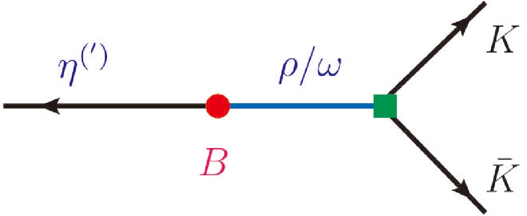
$ \rho(770) $ ,$ \omega(782) $ and their excited states for the decays$ B\to \pi K\bar K $ and$ B\to K K\bar K $ have been systematically studied [25] within the PQCD approach. However, the contributions of the subprocesses$ \rho(770,1450,1700) \to K \bar{K} $ and$ \omega(782,1420,1650)\to K \bar{K} $ remain missing for the three-body decays$ B\to \eta^{(\prime)} K\bar{K} $ . In this study, we assemble the blocks completely. The schematic view for the cascade decays$ B\to\eta^{(\prime)} \rho/ \omega\to \eta^{(\prime)}K\bar{K} $ , where$ \rho/\omega $ represents the intermediate states$ \rho(770,1450,1700) $ or$ \omega(782,1420,1650) $ that will decay into the kaon pair in this work, is shown in Fig. 1. The intermediate states in relevant cascade decays are generated in the hadronization of the quark-antiquark pair$ q\bar{q}^{(\prime)} $ , where$ {q}^{(\prime)} $ represents a u- or d-quark. The subprocesses of$ \rho\to K\bar{K} $ and$ \omega\to K\bar{K} $ which cannot be calculated in PQCD will be introduced into decay amplitudes via the kaon vector timelike form factors. The kaon vector timelike form factors are related to its electromagnetic form factors [67], which have been extensively studied in Refs. [63, 68−71] on the theoretical side and measured in the reactions$ e^+e^- \to K^+K^- $ [43, 44, 49] and$ e^+e^- \to K^+K^-(\gamma) $ [46]. A detailed discussion for the kaon vector timelike form factors as well as their coefficients are provided in Ref. [25]. The analyses for relevant three-body B meson decays within the symmetries one are referred to Refs. [72−80]; related papers within QCD factorization can be found in Refs. [67, 68, 81−97].
Figure 1. (color online) Schematic of the cascade decays
$ B\to\eta^{(\prime)} \rho/\omega \to \eta^{(\prime)}K\bar{K} $ , where$ \rho/\omega $ represents the intermediate states$ \rho(770,1450,1700) $ or$ \omega(782,1420,1650) $ that will decay into the kaon pair.This remainder of this paper is organized as follows. In Sec. II, we briefly describe the theoretical framework for the concerned quasi-two-body B meson decays within the PQCD approach and provide an expression for the differential branching fraction. In Sec. III, we present our numerical results for the CP averaged branching fractions and corresponding CP asymmetries for relevant quasi-two-body decay processes as well as some necessary discussions. A summary and conclusions of this work are provided in Sec. IV. The wave functions for the initial and final states and the factorization formulas for the related decay amplitudes are collected in Appendix A.
-
For the
$ B\to\eta^{(\prime)} \rho/\omega \to \eta^{(\prime)}K\bar{K} $ decays, the weak effective Hamiltonian can be specified as [1]$ \begin{aligned}[b] {\cal{H}}_{{\rm{eff}}} = \;&\frac{G_{\rm F}}{\sqrt{2}} \Biggr\{ V_{ub} V_{ud(s)}^* \Big[ C_1(\mu) O_1(\mu) + C_2(\mu) O_2(\mu) \Big] \\ \;&- V_{tb} V_{td(s)}^* \Biggr[ \sum\limits_{i=3}^{10} C_i(\mu) O_i(\mu) \Biggr] \Biggr\} + {\rm{H.c.}}, \end{aligned} $
(1) where
$ G_{\rm F} $ represents the Fermi coupling constant and$ V_{ub,uq,tb,tq} $ $ (q=d,s) $ represent the CKM matrix elements.$ C_i(\mu) $ are Wilson coefficients at the renormalization scale μ. In this study, we employ the renormalization group evolution of the Wilson coefficients from higher scale to lower scale as specified in Ref. [15], wherein the values of the Wilson coefficients at the$ m_b $ scale are$ \begin{aligned}[b] &C_1=-0.27034,\; \; C_2 = 1.11879,\; \; C_3 = 0.01261,\; \;\\ \;&C_4 = -0.02695,\; \; C_5 = 0.00847, \end{aligned} $
(2) $ \begin{aligned}[b] &C_6=-0.03260,\; \; C_7 = 0.00109,\; \; \\ \;&C_8 = 0.00040,\; \; C_9 = -0.00895,\; \; C_{10} = 0.00216. \end{aligned} $
(3) For the local four-quark operators
$ O_i $ , one has [1](1) Current-current operators
$ \begin{aligned} { \begin{array}{ll} O_1\, =\, (\bar{q}_\alpha u_\beta)_{V-A}(\bar{u}_\beta b_\alpha)_{V-A} , \ \ O_2\, =\, (\bar{q}_\alpha u_\alpha)_{V-A}(\bar{u}_\beta b_\beta)_{V-A} ; \end{array}} \end{aligned} $
(4) (2) QCD penguin operators
$ \begin{aligned}[b] \;& O_3\, =\, (\bar{q}_\alpha b_\alpha)_{V-A}\displaystyle\sum\limits_{q'}(\bar{q}'_\beta q'_\beta)_{V-A}\;, \\ & O_4\, =\, (\bar{q}_\alpha b_\beta)_{V-A}\displaystyle\sum\limits_{q'}(\bar{q}'_\beta q'_\alpha)_{V-A}\;, \\ \;& O_5\, =\, (\bar{q}_\alpha b_\alpha)_{V-A}\displaystyle\sum\limits_{q'}(\bar{q}'_\beta q'_\beta)_{V+A}\;, \\ & O_6\, =\, (\bar{q}_\alpha b_\beta)_{V-A}\displaystyle\sum\limits_{q'}(\bar{q}'_\beta q'_\alpha)_{V+A}\;; \end{aligned} $
(5) (3) Electroweak penguin operators
$ \begin{aligned}[b] \;& O_7\, =\, \frac{3}{2}(\bar{q}_\alpha b_\alpha)_{V-A}\sum\limits_{q'}e_{q'}(\bar{q}'_\beta q'_\beta)_{V+A}\;,\\ & O_8\, =\, \frac{3}{2}(\bar{q}_\alpha b_\beta)_{V-A}\sum\limits_{q'}e_{q'}(\bar{q}'_\beta q'_\alpha)_{V+A}\;, \\ \;& O_9\, =\, \frac{3}{2}(\bar{q}_\alpha b_\alpha)_{V-A}\sum\limits_{q'}e_{q'}(\bar{q}'_\beta q'_\beta)_{V-A}\;,\\ & O_{10}\, =\, \frac{3}{2}(\bar{q}_\alpha b_\beta)_{V-A}\sum\limits_{q'}e_{q'}(\bar{q}'_\beta q'_\alpha)_{V-A}\;. \end{aligned} $
(6) The subscripts
$ \alpha, \ \beta $ are the color indices and the notations$ (\bar{q}'q')_{V\pm A} $ represent$ \bar q' \gamma_\mu (1\pm \gamma_5)q' $ with the index$ q'=u,\;d,\;s $ .The theoretical analyses of B meson decays are performed in the B meson rest frame [98−103]. This is because working in this frame provides a clear physical picture in which final-state particles move fast in different directions and eliminates the effects of the intrinsic momentum of the B-meson in the calculations of decay amplitudes and integrals of phase space. Meanwhile, it is convenient to define the momenta for the initial and final states in the light-cone coordinates for B meson decays in the PQCD approach [13−16]. Subsequently, the momentum of
$ B^+, B^0 $ , or$ B^0_s $ for the decays considered in this work with mass$ m_B $ can be written as$ \begin{aligned} p_B=\frac{m_B}{\sqrt2}(1,1,0_{\rm{T}}) \end{aligned} $
(7) in the B meson rest frame. In return, one has the momenta
$ \begin{aligned} p_3&=\frac{m_B}{\sqrt2}(1-\zeta, 0, 0_{\rm{T}}), \end{aligned} $
(8) $ \begin{aligned} p&=\frac{m_B}{\sqrt 2}(\zeta, 1, 0_{\rm{T}}) \end{aligned} $
(9) for the bachelor state
$ \eta^{(\prime)} $ and$ K\bar K $ system originating from resonances ρ, ω, or their excited states, respectively. For the spectator quarks in the B meson,$ \eta^{(\prime)} $ , and the intermediate states, one has their momenta$ k_B=(\dfrac{m_B}{\sqrt2}x_B, 0, k_{B{\rm{T}}}) $ ,$ k_3=(\dfrac{m_B}{\sqrt2}(1-\zeta)x_3, 0, k_{3{\rm{T}}}) $ , and$ k= (0, \dfrac{m_B}{\sqrt 2}z, k_{\rm{T}}) $ accordingly. In addition, one needs to write down a longitudinal polarization vector$ \begin{aligned} \epsilon_L=\frac{1}{\sqrt 2}(-\sqrt\zeta, 1/\sqrt\zeta, 0_{\rm{T}}) \end{aligned} $
(10) for the resonances involved, which satisfies the relation
$ \epsilon_L \cdot p= 0 $ . The fractions$ x_B $ , z, and$ x_3 $ in the momenta will run from zero to one in the numerical calculation of this work. It is easy to check that the variable$ \zeta=s/m^2_B $ , when one defines the invariant mass square$ s=m^2_{K\bar K}\equiv p^2 $ .For subprocesses
$ \rho(770,1450,1700)\to K \bar{K} $ and$ \omega(782, 1420,1650)\to K \bar{K} $ , the corresponding electromagnetic form factors with the components of$ \rho, \omega $ and ϕ resonances and their excited states are written as [69]$ \begin{aligned}[b] F_{K^+}(s)=&+\frac12\sum\limits_{\iota=\rho,\rho^\prime,...} c^K_\iota {\rm{BW}}_\iota(s) +\frac16\sum\limits_{\varsigma=\omega,\omega^\prime,...} c^K_\varsigma {\rm{BW}}_\varsigma(s) \\ &+\frac13\sum\limits_{\kappa=\phi,\phi^\prime,..} c^K_\kappa {\rm{BW}}_\kappa(s), \end{aligned} $
(11) $ \begin{aligned}[b] F_{K^0}(s)=&-\frac12\sum\limits_{\iota=\rho,\rho^\prime,...} c^K_\iota {\rm{BW}}_\iota(s) +\frac16\sum\limits_{\varsigma=\omega,\omega^\prime,...} c^K_\varsigma {\rm{BW}}_\varsigma(s) \\ &+\frac13\sum\limits_{\kappa=\phi,\phi^\prime,..} c^K_\kappa {\rm{BW}}_\kappa(s), \quad \end{aligned} $
(12) which are defined by [69]
$ \begin{aligned} \langle K^+(p_1) K^-(p_2) | j^{em}_\mu | 0 \rangle &= (p_1-p_2)_\mu \,F_{K^+}(s), \end{aligned} $
(13) $ \begin{aligned} \langle K^0(p_1)\bar K^0(p_2) | j^{em}_\mu | 0 \rangle &= (p_1-p_2)_\mu\,F_{K^0}(s), \end{aligned} $
(14) where
$ \rho^\prime, \omega^{\prime} $ stand for$ \rho(1450), \omega(1420) $ , and the electromagnetic current$ j^{em}_\mu=\dfrac23\bar u\gamma_\mu u-\dfrac13\bar d\gamma_\mu d-\dfrac13\bar s\gamma_\mu s $ carried by the light quarks$ u, d $ and s [104]. The state ϕ and its excited states are embodied in components for the form factors$ F_{K^+}(s) $ and$ F_{K^0}(s) $ ; however, we are not concerned about the subprocess$ \phi(1020)\to K\bar{K} $ in this work because this decay is a natural decay mode compared to the$ \rho(770) $ and$ \omega(782) $ decay into$ K\bar{K} $ .The electromagnetic form factors
$ F_{K^+} $ and$ F_{K^0} $ can be separated into the isospin$ I=0 $ and$ I=1 $ components as$ F_{K^{+(0)}}=F_{K^{+(0)}}^{I=1} + F_{K^{+(0)}}^{I=0} $ , with the$ F_{K^+}^{I=0}=F_{K^0}^{I=0} $ and$ F_{K^+}^{I=1}= -F_{K^0}^{I=1} $ , and one has$ \langle K^+(p_1) \bar{K}^0(p_2) | \bar u \gamma_\mu d | 0 \rangle = (p_1- p_2)_\mu 2F_{K^+}^{I=1}(s) $ [69, 105]. Considering only the contribution for$ {K^+K^-} $ and$ {K^0\bar K^0} $ from the resonant states$\iota= \rho(770,$ $ 1450,1700) $ and$ \varsigma=\omega(782,1420,1650) $ , we have [67]$ \begin{aligned}[b] F_{K^+K^-}^{u}(s)=&F_{K^0\bar K^0}^{d}(s)= +\frac12\sum\limits_{\iota} c^K_\iota {\rm{BW}}_\iota(s) \\ \;&+\frac12\sum\limits_{\varsigma} c^K_\varsigma {\rm{BW}}_\varsigma(s), \end{aligned} $
(15) $ \begin{aligned}[b] F_{K^+K^-}^{d}(s)=&F_{K^0\bar K^0}^{u}(s)=-\frac12\sum\limits_{\iota} c^K_\iota {\rm{BW}}_\iota(s) \\ \;&+\frac12\sum\limits_{\varsigma} c^K_\varsigma {\rm{BW}}_\varsigma(s). \end{aligned} $
(16) For the
$ K^+\bar K^0 $ and$ K^0K^- $ pairs in the final states of the concerned decays in this work which will have no contribution from the neutral resonances$ \omega(782,1420,1650) $ , one has [63, 68, 69]$ \begin{aligned} F_{K^+\bar K^0}(s)=F_{K^0K^-}(s)&=F_{K^+}(s)-F_{K^0}(s) =\sum\limits_{\iota} c^K_\iota {\rm{BW}}_\iota(s), \end{aligned} $
(17) where
$ {\iota} $ represents the only component of the ρ family resonances.The coefficient
$ c^K_R $ in$ F_{K^{+,0}}(s) $ is proportional to the coupling constant$ g_{R K\bar K} $ , where R represents a resonance$ \rho(770,1450,1700) $ or$ \omega(782,1420,1650) $ in this work. The values for the related coefficients have been discussed in detail in Ref. [25]. In the numerical calculation of this work, we adopt the values$ \begin{aligned}[b] c^K_{\rho(770)}&=1.247\pm0.019, \\ c^K_{\omega(782)}&=1.113\pm0.019, \\ c^K_{\rho(1450)}&=-0.156\pm0.015, \\ c^K_{\omega(1420)}&=-0.117\pm0.013, \\ c^K_{\rho(1700)}&=-0.083\pm0.019, \\ c^K_{\omega(1650)}&=-0.083\pm0.019, \end{aligned} $
(18) as they are in [25] for the coefficients in the form factors
$ F_{K^{+}}(s) $ and$ F_{K^{0}}(s) $ .The BW formula in
$ F_{K^{+,0}}(s) $ has the form [106–107]$ \begin{aligned} {\rm{BW}}_R= \frac{m_{R}^2}{m_R^2-s- {\rm i} m_R \Gamma_{R}(s)}\,, \end{aligned} $
(19) where R represents the corresponding intermediate state, and the s-dependent width is given by
$ \begin{aligned} \Gamma_{R}(s) =\Gamma_R\frac{m_R}{\sqrt s} \frac{ \left| \overrightarrow{q} \right|^3}{ \left| \overrightarrow{q_0}\right|^3} X^2\left(\left| \overrightarrow{q} \right| r^R_{\rm{BW}}\right). \end{aligned} $
(20) The Blatt-Weisskopf barrier factor [108] is given by
$ \begin{aligned} X(z)=\sqrt{\frac{1+z^2_0}{1+z^2}}, \end{aligned} $
(21) with the barrier radius
$ r^R_{\rm{BW}}=4.0 $ GeV–1 as in Refs. [107, 109−112]. The magnitude of the momentum$ \begin{aligned} \left| \overrightarrow{q} \right|&=\frac{1}{2\sqrt s}\sqrt{\left[s-(m_K+m_{\bar K})^2\right] \left[s-(m_K-m_{\bar K})^2\right]}\,, \end{aligned} $
(22) and the
$ \left| \overrightarrow{q_0}\right| $ is$ \left| \overrightarrow{q} \right| $ at$ s=m^2_R $ .For the CP averaged differential branching fraction (
$ {\cal{B}} $ ) of the concerned quasi-two-body decays, we have the formula [23, 86, 113]$ \begin{aligned} \frac{{\rm d}{\cal{B}}}{{\rm d}\zeta}=\tau_B\frac{\left| \overrightarrow{q} \right|^3 \left| \overrightarrow{q_h}\right|^3} {12\pi^3m^5_B}\overline{|{\cal{A}}|^2}\;, \end{aligned} $
(23) with
$ \tau_B $ representing the mean lifetime of B meson. The factorization formula for the decay amplitude$ {\cal{A}} $ for the quasi-two-body decays$ B\to \eta^{(\prime)} [\rho/\omega\to] K\bar K $ is written as [114–115]$ \begin{aligned} {\cal{A}}=\phi_B \otimes {\cal{H}} \otimes \phi^{P{\text{-wave}}}_{K\bar K} \otimes \phi_{h} \end{aligned} $
(24) in the PQCD approach. The hard kernel
$ {\cal{H}} $ contains only one hard gluon exchange at the leading order in the strong coupling$ \alpha_s $ according to Fig. A1 in Appendix A. The symbol$\otimes $ indicates convolutions in parton momenta. Distribution amplitudes$ \phi_B $ ,$ \phi_{h} $ , and$\phi^{P{\text{-wave}}}_{K\bar K}$ and their input parameters as well as Lorentz invariant decay amplitudes for decays$ B\to \eta^{(\prime)} [\rho/\omega\to] K\bar K $ are provided in Appendix A. The magnitude of the momentum$ |\overrightarrow{q_{h}}| $ for the meson$ h=\eta^{(\prime)} $ in the rest frame of the resonance is written as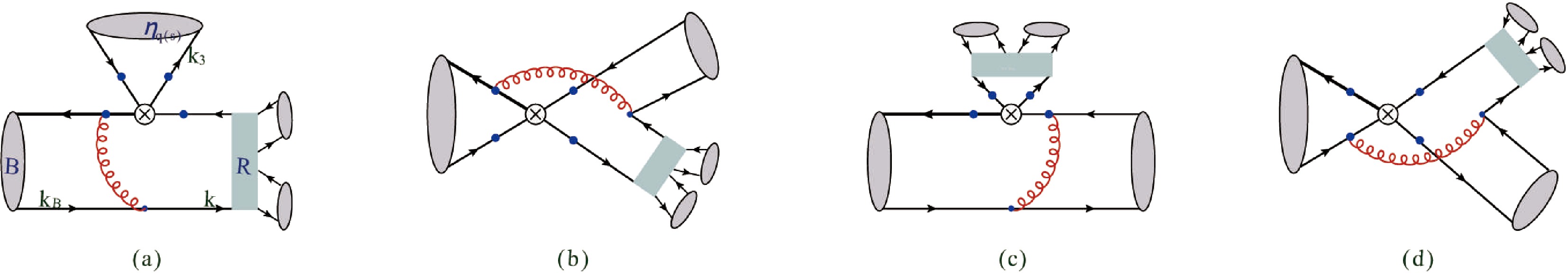
Figure A1. (color online) Typical Feynman diagrams for processes
$ B\to\eta_{q(s)} R \to \eta_{q(s)} K\bar K $ , where R represents the resonances ρ and ω and their excited states. The dots on the quarks connecting the weak vertex$ \otimes $ are the switchable vertices for the hard gluons.$ \begin{aligned} \left| \overrightarrow{q_h}\right|=\frac{1}{2\sqrt s} \sqrt{\left[m^2_{B}-(\sqrt s+m_{h})^2\right]\left[m^2_{B}-(\sqrt s-m_{h})^2\right]}, \end{aligned} $
(25) where
$ m_h $ represents the mass for the bachelor meson$ \eta^{(\prime)} $ . When we face the meson pairs$ K^+K^- $ and$ K^0\bar{K}^0 $ in the final states, Eq. (22) has a simpler form$ \begin{aligned} \left| \overrightarrow{q} \right|&=&\frac{1}{2}\sqrt{s-4m_K^2}\,. \end{aligned} $
(26) The direct CP asymmetry
${\cal{A}}_{\rm CP}$ for the decays in this work is defined as$ \begin{aligned} {\cal{A}}_{\rm CP}=\frac{{\cal{B}}(\bar B\to \bar f)-{\cal{B}}(B\to f)}{{\cal{B}}(\bar B\to \bar f)+{\cal{B}}(B\to f)}. \end{aligned} $
(27) -
In the numerical calculation in this study, we adopt the values
$ f_B=0.190 $ GeV and$ f_{B_s}=0.230 $ GeV for the decay constants of the$ B^{\pm,0} $ and$ B^0_s $ mesons [113], respectively. For these B mesons, their mean lifetimes are$ \tau_{B^\pm}=1.638 \times 10^{-12} $ s,$ \tau_{B^0}=1.517 \times 10^{-12} $ s and$ \tau_{B^0_s}= 1.520 \times 10^{-12} $ s [113]. The other inputs for the numerical results are presented in Table 1.$ m_{B^{\pm}}=5.279 $ $ m_{B^{0}}=5.280 $ $ m_{B^0_s}\,=5.367 $ $ m_{\pi^{\pm}}=0.140 $ $ m_{\pi^0}\,=0.135 $ $ m_{K^{\pm}}=0.494 $ $ m_{K^{0}}=0.498 $ $ m_{\eta}=0.548 $ $ m_{\eta^{'}} =0.958 $ $ m_{\rho(770)}=0.775 $ $ \Gamma_{\rho(770)}=0.147 $ $ m_{\omega(782)}=0.783 $ $ \Gamma_{\omega(782)}=0.00868 $ $ m_{\rho(1450)}=1.465\pm0.025 $ $ \Gamma_{\rho(1450)}=0.400\pm0.060 $ $ m_{\omega(1420)}=1.410\pm0.060 $ $ \Gamma_{\omega(1420)}=0.290\pm0.190 $ $ m_{\rho(1700)}=1.720\pm0.020 $ $ \Gamma_{\rho(1700)}=0.250\pm0.100 $ $ m_{\omega(1650)}=1.670\pm0.030 $ $ \Gamma_{\omega(1650)}=0.315\pm0.035 $ $ \lambda=0.22501\pm 0.00068 $ $ A=0.826^{+0.016}_{-0.015} $ $ \bar{\rho} = 0.1591\pm0.0094 $ $ \bar{\eta}= 0.3523^{+0.0073}_{-0.0071} $ Table 1. Inputs from [113]: Masses for the relevant particles, full widths for
$ \rho$ (770, 1450, 1700) and$ \omega(782, 1420, $ $ 1650) $ (in units of GeV), and the Wolfenstein parameters.Utilizing the decay amplitudes reported in Appendix A and the differential branching fractions in Eq. (23), it is trivial to obtain the CP averaged branching fractions and direct CP asymmetries for the concerned quasi-two-body decay processes
$ B\to \eta^{(\prime)} \rho(770, 1450,1700)\to \eta^{(\prime)}K\bar K $ and$ B\to\eta^{(\prime)}\omega(782,1420, 1650) \to \eta^{(\prime)}K\bar K $ , as shown in Tables 2, 3, and 4. Owing to the small mass difference between$ K^\pm $ and$ K^0 $ , the branching fractions or direct$\rm CP$ asymmetries for the specific quasi-two-body decays$ B\to \eta^{(\prime)}R\to \eta^{(\prime)}K^0\bar K^0 $ and$ B\to \eta^{(\prime)}R\to \eta^{(\prime)}K^+K^- $ are very close, where the intermediate state R is in these resonances$ \rho(770,1450,1700)^0 $ and$ \omega(782,1420,1650) $ . Consequently, we omit the corresponding results for those quasi-two-body decays with the subprocesses$ \rho(770, 1450, 1700)^0\to K^0\bar K^0 $ and$ \omega(782, 1420, 1650)\to K^0\bar K^0 $ in Tables 2, 3, and 4. We need to stress here that, the$ K^0\bar K^0 $ in the final states of the decays considered in this study with the P-wave resonant origin cannot produce$ K^0_SK^0_S $ or$ K^0_LK^0_L $ pairs.Decay modes $ {\cal{B}} $ ${\cal{A} }_{\rm CP}$ $ B^+ \to \eta [\rho(770)^+ \to] K^+ \bar K^0 $ $ 8.03^{+1.69+1.75+0.47+0.25+0.40+0.19}_{-2.31-2.09-0.47-0.24-0.35-0.10} \times 10^{-8} $ $ 0.00^{+0.00+0.01+0.01+0.00+0.00+0.00}_{-0.00-0.02-0.01-0.00-0.00-0.00} $ $ B^+ \to \eta{'} [\rho(770)^+ \to] K^+ \bar K^0 $ $ 5.01^{+1.07+0.99+0.41+0.15+0.24+0.02}_{-1.46-1.28-0.41-0.15-0.22-0.07} \times 10^{-8} $ $ 0.23^{+0.00+0.04+0.01+0.00+0.00+0.32}_{-0.01-0.03+0.01+0.00+0.00+0.32} $ $ B^0 \to \eta [\rho(770)^0 \to] K^+ K^- $ $ 1.51^{+0.26+0.95+0.09+0.05+0.07+0.17}_{-0.34-1.47-0.09-0.05-0.06-0.21} \times 10^{-9} $ $ 0.04^{+0.01+0.04+0.02+0.00+0.00+0.06}_{-0.02-0.03-0.02-0.00-0.00-0.06} $ $ B^0 \to \eta{'} [\rho(770)^0 \to] K^+ K^- $ $ 1.03^{+0.18+0.34+0.08+0.04+0.05+0.11}_{-0.24-0.90-0.07-0.03-0.04-0.12} \times 10^{-9} $ $ 0.64^{+0.00+0.39+0.02+0.00+0.00+0.43}_{-0.00-0.03-0.02-0.00-0.00-0.47} $ $ B^0 \to \eta [\omega(782) \to] K^+ K^- $ $ 1.41^{+0.22+0.30+0.08+0.05+0.07+0.19}_{-0.28-0.42-0.08-0.05-0.06-0.34} \times 10^{-9} $ $ 0.43^{+0.00+0.27+0.01+0.00+0.01+0.59}_{-0.00-0.20-0.01-0.00-0.01-0.60} $ $ B^0 \to \eta{'} [\omega(782) \to] K^+ K^- $ $ 9.36^{+1.57+3.39+1.03+0.32+0.46+1.14}_{-2.13-1.83-0.38-0.32-0.43-2.09} \times 10^{-10} $ $ 0.11^{+0.01+0.15+0.01+0.00+0.00+0.15}_{-0.00-0.37-0.01-0.00-0.00-0.15} $ $ B_s^0 \to \eta [\rho(770)^0 \to] K^+ K^- $ $ 3.16^{+0.92+0.24+0.33+0.10+0.13+0.28}_{-1.43-0.16-0.31-0.10-0.12-0.47} \times 10^{-10} $ $ -0.24^{+0.01+0.04+0.02+0.00+0.00+0.33}_{-0.02-0.04-0.02-0.00-0.00-0.33} $ $ B_s^0 \to \eta{'} [\rho(770)^0 \to] K^+ K^- $ $ 8.76^{+2.15+0.74+0.31+0.27+0.37+0.89}_{-3.17-0.73-0.29-0.27-0.35-1.34} \times 10^{-10} $ $ 0.12^{+0.01+0.02+0.00+0.00+0.00+0.16}_{-0.01-0.02-0.00-0.00-0.00-0.16} $ $ B_s^0 \to \eta [\omega(782) \to] K^+ K^- $ $ 3.08^{+0.90+0.22+0.32+0.11+0.13+0.28}_{-1.37-0.17-0.30-0.10-0.12-0.46} \times 10^{-10} $ $ -0.25^{+0.01+0.04+0.02+0.00+0.00+0.34}_{-0.02-0.04-0.02-0.00-0.00-0.34} $ $ B_s^0 \to \eta{'} [\omega(782) \to] K^+ K^- $ $ 8.46^{+2.08+0.71+0.29+0.29+0.36+0.86}_{-3.07-0.71-0.29-0.28-0.33-1.29} \times 10^{-10} $ $ 0.12^{+0.01+0.02+0.00+0.00+0.00+0.16}_{-0.01-0.02-0.00-0.00-0.00-0.16} $ Table 2. PQCD predictions of the
$\rm CP$ averaged branching fractions and direct$\rm CP$ asymmetries for the quasi-two-body$ B\to \eta^{(\prime)}\rho(770) \to \eta^{(\prime)}K\bar K $ and$ B\to \eta^{(\prime)}\omega(782) \to \eta^{(\prime)}K\bar K $ decays. The decays with the subprocess$ \rho(770)^0\to K^0\bar K^0 $ or$ \omega(782)\to K^0\bar K^0 $ have the same results as their corresponding decay modes with$ \rho(770)^0\to K^+K^- $ or$ \omega(782)\to K^+K^- $ .Decay modes $ {\cal{B}} $ ${\cal{A} }_{\rm CP}$ $ B^+ \to \eta [\rho(1450)^+ \to] K^+ \bar K^0 $ $ 5.49^{+1.18+1.13+0.32+1.00+0.26+0.27}_{-1.62-1.34-0.33-1.11-0.24-0.16} \times 10^{-8} $ $ 0.01^{+0.00+0.01+0.01+0.00+0.00+0.01}_{-0.00-0.01-0.01-0.00-0.00-0.01} $ $ B^+ \to \eta{'} [\rho(1450)^+ \to] K^+ \bar K^0 $ $ 3.47^{+0.77+0.66+0.29+0.02+0.16+0.16}_{-1.03-0.85-0.28-0.03-0.15-0.10} \times 10^{-8} $ $ 0.23^{+0.01+0.05+0.01+0.00+0.00+0.02}_{-0.01-0.03-0.01-0.00-0.00-0.10} $ $ B^0 \to \eta [\rho(1450)^0 \to] K^+ K^- $ $ 1.81^{+0.32+1.01+0.10+0.37+0.08+0.22}_{-0.40-1.95-0.11-0.37-0.07-0.19} \times 10^{-9} $ $ 0.00^{+0.01+0.02+0.02+0.00+0.00+0.00}_{-0.00-0.02-0.02-0.00-0.00-0.00} $ $ B^0 \to \eta{'} [\rho(1450)^0 \to] K^+ K^- $ $ 1.35^{+0.25+0.46+0.10+0.24+0.06+0.13}_{-0.30-1.49-0.09-0.28-0.05-0.12} \times 10^{-9} $ $ 0.65^{+0.00+0.45+0.02+0.00+0.00+0.04}_{-0.00-0.03-0.02-0.00-0.00-0.06} $ $ B^0 \to \eta [\omega(1420) \to] K^+ K^- $ $ 6.00^{+0.83+1.24+0.33+1.21+0.27+0.83}_{-1.05-1.74-0.34-1.37-0.26-2.03} \times 10^{-10} $ $ 0.45^{+0.01+0.27+0.01+0.00+0.01+0.11}_{-0.00-0.20-0.01-0.00-0.01-0.09} $ $ B^0 \to \eta{'} [\omega(1420) \to] K^+ K^- $ $ 4.00^{+0.64+1.15+0.30+0.84+0.20+0.57}_{-0.84-0.88-0.29-0.94-0.19-1.38} \times 10^{-10} $ $ 0.13^{+0.01+0.28+0.01+0.00+0.00+0.05}_{-0.00-0.36-0.01-0.00-0.01-0.02} $ $ B_s^0 \to \eta [\rho(1450)^0 \to] K^+ K^- $ $ 4.54^{+1.34+0.39+0.49+0.83+0.54+0.39}_{-2.09-0.30-0.45-0.92-0.60-0.68} \times 10^{-10} $ $ -0.24^{+0.02+0.05+0.03+0.00+0.00+0.05}_{-0.02-0.05-0.03-0.00-0.00-0.06} $ $ B_s^0 \to \eta{'} [\rho(1450)^0 \to] K^+ K^- $ $ 1.22^{+0.30+0.09+0.04+0.22+0.05+0.12}_{-0.45-0.09-0.04-0.25-0.05-0.17} \times 10^{-9} $ $ 0.14^{+0.01+0.02+0.00+0.00+0.00+0.02}_{-0.01-0.02-0.00-0.00-0.00-0.02} $ $ B_s^0 \to \eta [\omega(1420) \to] K^+ K^- $ $ 1.59^{+0.47+0.12+0.16+0.33+0.07+0.14}_{-0.72-0.11-0.16-0.37-0.06-0.24} \times 10^{-10} $ $ -0.24^{+0.01+0.05+0.03+0.00+0.00+0.05}_{-0.02-0.04-0.03-0.00-0.00-0.06} $ $ B_s^0 \to \eta{'} [\omega(1420) \to] K^+ K^- $ $ 4.04^{+1.02+0.29+0.15+0.85+0.17+0.39}_{-1.49-0.28-0.14-0.95-0.16-0.58} \times 10^{-10} $ $ 0.15^{+0.01+0.02+0.00+0.00+0.00+0.02}_{-0.01-0.02-0.00-0.00-0.00-0.02} $ Table 3. PQCD predictions of the
$\rm CP$ averaged branching fractions and direct$\rm CP$ asymmetries for the quasi-two-body$ B\to \eta^{(\prime)}\rho(1450) \to \eta^{(\prime)}K\bar K $ and$ B\to \eta^{(\prime)} \omega(1420) \to \eta^{(\prime)}K\bar K $ decays. Those decays with the subprocess$ \rho(1450)^0\to K^0\bar K^0 $ or$ \omega(1420)\to K^0\bar K^0 $ have the same results as their corresponding decay modes with$ \rho(1450)^0\to K^+K^- $ or$ \omega(1420)\to K^+K^- $ .Decay modes $ {\cal{B}} $ ${\cal{A} }_{\rm CP}$ $ B^+ \to \eta [\rho(1700)^+ \to] K^+ \bar K^0 $ $ 6.00^{+1.28+1.37+0.36+2.43+0.28+0.38}_{-1.72-1.62-0.35-3.06-0.27-0.25} \times 10^{-8} $ $ 0.00^{+0.00+0.01+0.01+0.00+0.00+0.00}_{-0.00-0.02-0.01-0.00-0.00-0.00} $ $ B^+ \to \eta{'} [\rho(1700)^+ \to] K^+ \bar K^0 $ $ 3.78^{+0.81+0.77+0.32+1.53+0.18+0.21}_{-1.11-1.01-0.31-1.93-0.17-0.14} \times 10^{-8} $ $ 0.24^{+0.01+0.05+0.01+0.00+0.00+0.02}_{-0.01-0.03-0.01-0.00-0.00-0.02} $ $ B^0 \to \eta [\rho(1700)^0 \to] K^+ K^- $ $ 2.11^{+0.38+1.40+0.12+0.85+0.09+0.30}_{-0.45-2.21-0.13-1.08-0.09-0.27} \times 10^{-9} $ $ -0.02^{+0.01+0.07+0.02+0.00+0.00+0.01}_{-0.01-0.05-0.02-0.00-0.00-0.01} $ $ B^0 \to \eta{'} [\rho(1700)^0 \to] K^+ K^- $ $ 7.89^{+1.44+2.55+0.57+3.20+0.34+0.83}_{-1.81-7.12-0.56-4.01-0.32-0.81} \times 10^{-10} $ $ 0.65^{+0.00+0.44+0.02+0.00+0.00+0.03}_{-0.00-0.03-0.02-0.00-0.00-0.06} $ $ B^0 \to \eta [\omega(1650) \to] K^+ K^- $ $ 6.81^{+1.04+1.44+0.39+2.76+0.32+1.12}_{-1.29-2.12-0.38-3.49-0.30-2.66} \times 10^{-10} $ $ 0.55^{+0.01+0.29+0.01+0.00+0.01+0.07}_{-0.00-0.20-0.01-0.00-0.01-0.07} $ $ B^0 \to \eta{'} [\omega(1650) \to] K^+ K^- $ $ 4.82^{+0.88+1.68+0.35+1.96+0.24+0.83}_{-0.98-0.96-0.35-2.45-0.23-1.96} \times 10^{-10} $ $ 0.19^{+0.00+0.21+0.01+0.00+0.01+0.06}_{-0.00-0.38-0.01-0.00-0.01-0.04} $ $ B_s^0 \to \eta [\rho(1700)^0 \to] K^+ K^- $ $ 4.40^{+1.33+0.50+0.52+1.79+0.19+0.37}_{-2.10-0.40-0.48-2.25-0.17-0.57} \times 10^{-10} $ $ -0.27^{+0.03+0.05+0.03+0.00+0.00+0.07}_{-0.03-0.05-0.03-0.00-0.00-0.07} $ $ B_s^0 \to \eta{'} [\rho(1700)^0 \to] K^+ K^- $ $ 1.31^{+0.33+0.05+0.04+0.53+0.06+0.12}_{-0.48-0.05-0.04-0.67-0.05-0.18} \times 10^{-9} $ $ 0.12^{+0.01+0.02+0.00+0.00+0.00+0.02}_{-0.01-0.02-0.00-0.00-0.00-0.02} $ $ B_s^0 \to \eta [\omega(1650) \to] K^+ K^- $ $ 1.54^{+0.47+0.16+0.17+0.78+0.06+0.13}_{-0.73-0.13-0.16-0.62-0.06-0.20} \times 10^{-10} $ $ -0.28^{+0.02+0.05+0.02+0.00+0.00+0.07}_{-0.02-0.05-0.04-0.00-0.00-0.08} $ $ B_s^0 \to \eta{'} [\omega(1650) \to] K^+ K^- $ $ 4.41^{+1.10+0.37+0.15+1.79+0.19+0.41}_{-1.62-0.35-0.15-2.25-0.17-0.61} \times 10^{-10} $ $ 0.12^{+0.01+0.02+0.00+0.00+0.00+0.02}_{-0.01-0.02-0.00-0.00-0.00-0.02} $ Table 4. PQCD predictions of the
$\rm CP$ averaged branching fractions and direct$\rm CP$ asymmetries for the quasi-two-body$ B\to \eta^{(\prime)}\rho(1700) \to \eta^{(\prime)}K\bar K $ and$ B\to \eta^{(\prime)}\omega(1650) \to \eta^{(\prime)}K\bar K $ decays. Those decays with the subprocess$ \rho(1700)^0\to K^0\bar K^0 $ or$ \omega(1650)\to K^0\bar K^0 $ have the same results as their corresponding decay modes with$ \rho(1700)^0\to K^+K^- $ or$ \omega(1650)\to K^+K^- $ .For these predicted results, the first error is induced from the uncertainties of the shape parameter
$ \omega_B = 0.40\pm0.04 $ and$ \omega_{B_s} = 0.50\pm 0.05 $ for the$ B^{+,0} $ and$ B^0_s $ meson. The second error comes from the uncertainties of the Gegenbauer moments$ a^0_R=0.25 \pm0.10 $ ,$ a^t_R=-0.50\pm 0.20 $ , and$ a^s_R=0.75\pm0.25 $ for the distribution amplitudes of the intermediate states in Eqs. (A10)−(A12), respectively. The$ \eta-\eta{'} $ mixing angle$ \phi=(40.0\pm2.0_{\rm{stat}}\pm0.6_{\rm{syst}})^{\circ} $ contributes the third error. The fourth and fifth errors originate from the coefficient$ c^K_R $ of$ F_{K^{+,0}}(s) $ in Eq. (18) and the Wolfenstein parameters in Table 1, respectively. The last error arises from the hard scale t with the range of$ 0.75t $ to$ 1.25t $ and the QCD scale$\Lambda_{\rm QCD}=0.25\pm0.05$ GeV with reference to [116]. There are other errors for the results in this work, which can be attributed to the uncertainties of the masses and the decay constants of the initial and final states, and the chiral scale parameters of the bachelor mesons, etc., are small and neglected.The branching fraction and direct CP asymmetry for the two-body decay
$ B^+ \to \eta \rho(770)^+ $ were averaged in [113] with$ {{\cal{B}}}=(7.0\pm2.9) \times 10^{-6} $ and$ {{\cal{A}}}_{\rm CP}=0.11\pm 0.11 $ from the original results$ {{\cal{B}}}=(9.9\pm1.2\pm0.8) \times 10^{-6} $ and$ {{\cal{A}}}_{\rm CP}=0.13\pm0.11\pm0.02 $ and$ {{\cal{B}}}=(4.1^{+1.4}_{-1.3}\pm0.4) \times 10^{-6} $ and${{\cal{A}}}_{\rm CP}=-0.04^{+0.34}_{-0.32}\pm0.01$ presented by the BABAR and Belle collaborations in [117] and [118], respectively. To illustrate the capabilities of the method adopted in this study, we calculate the branching fraction and direct CP asymmetry for the quasi-two-body decay$ B^+ \to \eta \rho(770)^+ \to \eta \pi^+\pi^0 $ with the results$ \begin{aligned} {{\cal{B}}}&=(6.34^{+1.73}_{-2.20}) \times 10^{-6}, \end{aligned} $
(28) $ \begin{aligned} {{\cal{A}}}_{\rm CP}&=-0.006^{+0.006}_{-0.010}, \end{aligned} $
(29) where individual errors have been added in quadrature. Apparently, our predictions are consistent with the corresponding data in [113] for the two-body decay
$ B^+ \to \eta \rho(770)^+ $ in view of$ {{\cal{B}}}( \rho(770)^+ \to \pi^+\pi^0)\approx $ 100% [113].The coupling constants
$ g_{\rho(1450)^0\pi^+\pi^-} $ and$ g_{\rho(1450)^0K^+K^-} $ can be achieved by$ \begin{aligned} g_{\rho(1450)^0h^+h^-}=\sqrt{\frac{6\pi m^2_{\rho(1450)}\Gamma_{\rho(1450)}{\cal{B}}_{\rho(1450)^0\to h^+h^-}}{q^3}}\,, \end{aligned} $
(30) where h is a pion or kaon, and
$ q=\dfrac{1}{2}\sqrt{m^2_{\rho(1450)}-4m_h^2} $ . According to the relationship$ g_{\rho(1450)^0K^+K^-}\approx \dfrac12 g_{\rho(1450)^0\pi^+\pi^-} $ [69] one has the ratio [23]$ \begin{aligned}[b] R_{\rho(1450)} &= \frac{{\cal{B}}(\rho(1450)^0\to K^+ K^-)}{{\cal{B}}(\rho(1450)^0 \to\pi^+\pi^-)} \\ \;&\approx \frac{g^2_{\rho(1450)^0K^+K^-} (m^2_{\rho(1450)}-4m^2_K)^{3/2}} {g^2_{\rho(1450)^0\pi^+\pi^-}(m^2_{\rho(1450)}-4m^2_\pi)^{3/2}} \\ &= 0.107. \end{aligned} $
(31) Since the pole mass of
$ \rho(770) $ is smaller than that of the kaon pair, it is not appropriate to calculate the ratio$ R_{\rho(770)} $ through a similar formula. Considering the smaller phase space available in$ \rho(770)\to K\bar K $ relative to$ \rho(770)\to \pi\pi $ , along with the ratio$ R_{\rho(1450)} $ , it is easy to understand the branching fraction in Table 2 for the quasi-two-body decay process$ B^+\to\eta [\rho(770)^+ \to] K^+ \bar K^0 $ , which is two orders smaller than the data in [113] for the two-body decay$ B^+ \to\eta\rho(770)^+ $ .From the branching fractions in Tables 2 and 3, the virtual contributions for the kaon pair from the BW tails of the resonances
$ \rho(770) $ and$ \omega(782) $ are on the order of or larger than the corresponding contributions from$ \rho(1450) $ and$ \omega(1420) $ . However, owing to the relatively smaller value for the$ c^K_{\omega(1420)} $ than that for$ c^K_{\rho(1450)} $ adopted in this study, the ratio of the branching fractions for a concerned quasi-two-body decay with the subprocesses$ \omega(1420)\to K\bar{K} $ and$ \omega(782)\to K\bar{K} $ is obviously smaller than the ratio of that with the$ \rho(1450)\to K\bar{K} $ and$ \rho(770)\to K\bar{K} $ . While the branching fractions in Table 4 with the subprocesses$ \rho(1700)\to K\bar{K} $ and$ \omega(1650)\to K\bar{K} $ are comparable to their corresponding branching fractions in Table 3, which can be attributed to the contribution of the resonances$ \rho(1450) $ and$ \omega(1420) $ for the kaon pair.In Fig. 2, we show the differential branching fractions for the decays
$ B^+\to \eta [\rho(770)^+\to] K^+\bar{K}^0 $ and$ B^+\to \eta [\rho(770)^+\to] \pi^+\pi^0 $ . To provide a good contrast, we magnify the value of each point of the solid line for$ B^+\to \eta [\rho(770)^+\to] K^+\bar{K}^0 $ by a factor of$ 10 $ in the diagram. The inset in Fig. 2 shows that the differential branching fraction for$ B^+\to \eta [\rho(770)^+\to] K^+\bar{K}^0 $ , which is related to the virtual contribution, does not appear as a typical BW curve for the normal quasi-two-body decay process like$ B^+\to \eta [\rho(770)^+\to] \pi^+\pi^0 $ . A broad bump is found for the process$ B^+\to \eta [\rho(770)^+ \to] K^+\bar{K}^0 $ with its peak at about$ \sqrt{s}=1.35 $ GeV. This bump does not represent the mass for a new resonance; it is generated from the BW tail of$ \rho(770)^+ $ along with a strong suppression factor$ \left| \overrightarrow{q_h}\right|^3 $ in Eq. (23). Further, we find that the curve for the differential branching fraction with the virtual contribution involved is not significantly affected by the decay width of the related intermediate state, which is surprising. In fact, the imaginary part of the denominator in the BW formula for$ \rho(770) $ (or$ \omega(782) $ ), which holds the energy dependent width of the intermediate state, is expected to become unimportant when the invariant mass square for kaon pair is sufficiently large. Then, the BW expression is charged only by the coefficient$ c^K_R $ in the time-like form factors for kaons in this study as well as by the gap between the s and squared mass$ m^2_R $ for the intermediate state. The threshold for the kaon pair is not far from the pole masse of$ \rho(770) $ (or$ \omega(782) $ ); therefore, because of the strong suppression from the factor$ \left| \overrightarrow{q}\right|^3 $ in Eq. (23), the differential branching fraction with the subprocess$ \rho(770)^+\to K^+\bar{K}^0 $ reaches its peak at about$ 1.35 $ GeV as shown in Fig. 2.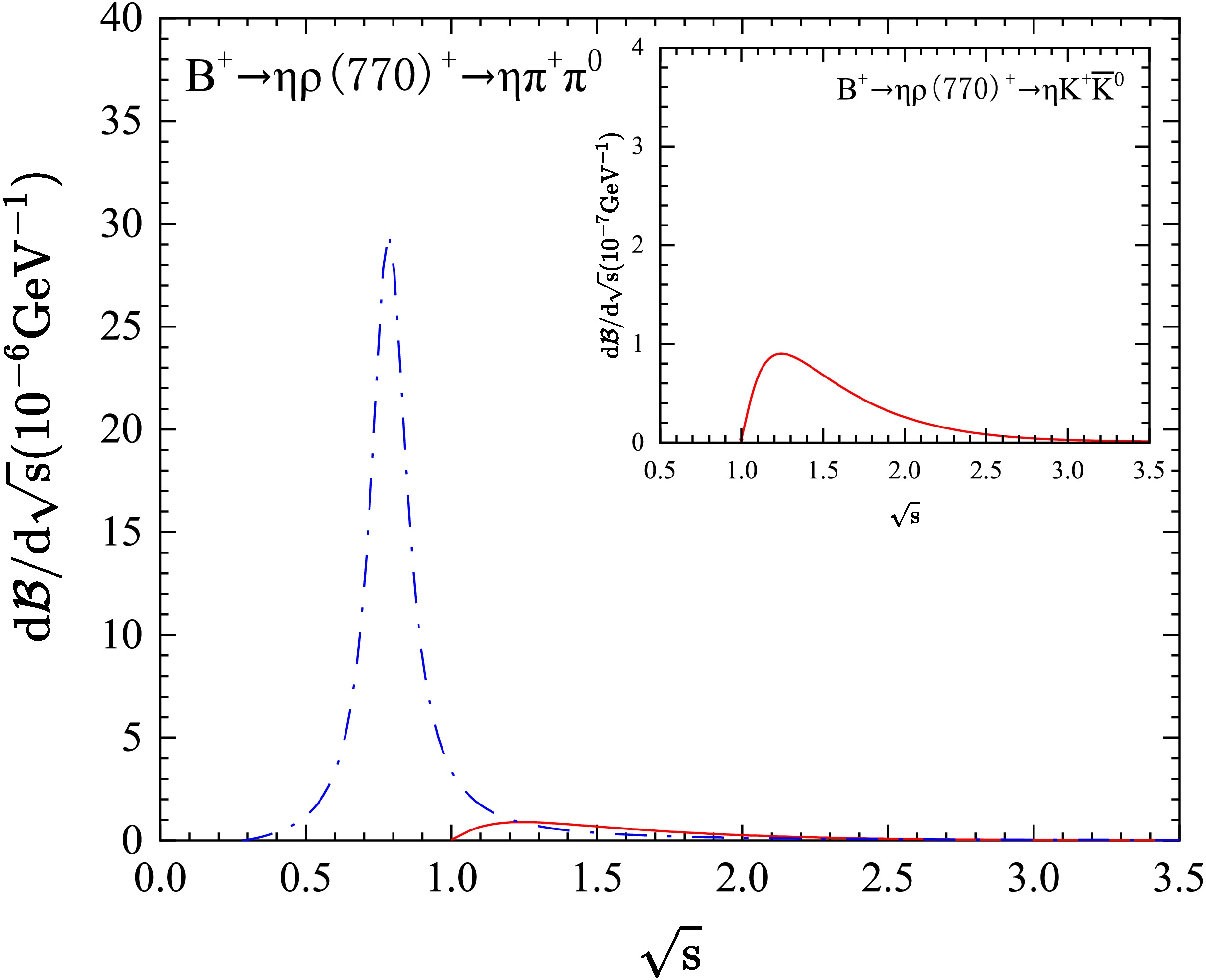
Figure 2. (color online) Differential branching fractions for the decays
$ B^+\to \eta [\rho(770)^+\to] K^+\bar{K}^0 $ and$ B^+\to \eta [\rho(770)^+\to] \pi^+\pi^0 $ . The inset is provided for comparison between the differential branching fractions of$ B^+\to \eta [\rho(770)^+\to] K^+\bar{K}^0 $ and$ B^+\to $ $ \eta [\rho(770)^+\to] \pi^+\pi^0 $ , in which the solid line for$ B^+\to \eta [\rho(770)^+\to] $ $ K^+\bar{K}^0 $ is magnified by a factor of$ 10 $ .In principle, the perturbative QCD calculations are applicable when the energy release is sufficiently large. Therefore, testing the reliability of the PQCD framework in the high-mass range is essential. Fortunately, the evolution of the time-like form factor
$ F_{K\bar K}(s) $ in the decay amplitude$ {\cal A} $ and phase space factor$ | \overrightarrow{q_h}| $ in the differential branching fraction of Eq. (23) naturally suppresses the resonant contribution from the region where the invariant mass of the kaon pair is considerably higher than the pole mass of the resonance. Considering$ B^+ \to \eta [\rho(770)^+ \to] K^+ \bar K^0 $ as an example, the main portion of its branching ratio is found to lie in the mass region around$ 1.35 $ GeV, as shown in Fig. 2. Numerically, the central values of its branching ratio are calculated as$ 5.69 \times 10^{-8} $ and$ 6.78 \times 10^{-8} $ when the$ K^+ \bar K^0 $ invariant mass upper limit is set to$ 2.0 $ GeV and$ 2.5 $ GeV, respectively; this amounts to 70.86% and 84.43% of the value$ 8.03 \times 10^{-8} $ , as indicated in Table 2. The similar ratios become 84.88% and 93.81% for$ B^+ \to \eta [\rho(1450)^+ \to] K^+ \bar K^0 $ , and 84.17% and 95.00% for$ B^+ \to \eta [\rho(1700)^+ \to] K^+ \bar K^0 $ . These results indicate that these considered resonance contributions primarily originate from the low invariant mass region. Meanwhile, compared to the contribution for a full resonance, the high invariant mass region has a more significant impact on the contribution for the off-shell state. On the whole, it validates the reliability of the PQCD predictions for the processes in this study. -
In this study, we investigated the contributions of the subprocesses
$ \rho(770,1450,1700) \to K \bar{K} $ and$ \omega(782,1420, 1650)\to K \bar{K} $ in the three-body decays$ B\to \eta^{(\prime)} K\bar{K} $ by employing the perturbative QCD approach. The kaon vector time like form factors for the subprocesses of$ \rho\to K\bar{K} $ and$ \omega\to K\bar{K} $ , which are related to its electromagnetic form factors, were introduced into the distribution amplitudes for$ K\bar K $ system. The CP averaged branching fractions for the considered decays were predicted to be on the order of$ 10^{-10} $ to$ 10^{-8} $ . The contributions for the kaon pair from the BW tails of the resonances$ \rho(770) $ and$ \omega(782) $ were found to be on the order of or larger than the corresponding contributions from$ \rho(1450,1700) $ and$ \omega(1420,1650) $ . This indicates that those virtual contributions cannot be ignored in the$ K\bar{K} $ system. Further, we found that the curve for the differential branching fraction with the virtual contribution involved is not significantly affected by the decay width of the related intermediate state$ \rho(770) $ (or$ \omega(782) $ ). This is because the imaginary part of the denominator in the BW formula becomes unimportant when the invariant mass square for kaon pair is considerably larger that the pole mass of the resonance. The well-determined relative phase angles between the states of the ρ or ω family in the$ K\bar K $ form factor are currently lacking, along with the experimental measurement for the decays considered in this study. Therefore, the total branching fractions and CP asymmetries accounting for all resonant contributions and their interference effects in the concerned decays will be considered in future studies. All PQCD predictions in this study are expected to be measured in the future high-statistics experiments conducted by Belle II and LHCb. -
In three-body decays
$ B\to \eta^{(\prime)} K\bar{K} $ , the mixing between η and$ \eta^{\prime} $ are considered. The physical states η and$ \eta^\prime $ are made from$ \eta_q=(u\bar u+d\bar d)/\sqrt2 $ and$ \eta_s=s\bar s $ at the quark level in early studies [119–120] with$ \begin{aligned} \left(\begin{array}{c} \eta \\ \eta^{\prime} \end{array} \right) = \left(\begin{array}{cc} \cos{\phi} & -\sin{\phi} \\ \sin{\phi} & \cos{\phi} \\ \end{array} \right) \left(\begin{array}{c} \eta_q \\ \eta_s \end{array} \right), \end{aligned} $
(A1) where the mixing angle
$ \phi=39.3^{\circ}\pm1.0^{\circ} $ , and the decay constants$ f_{\eta_q}=(1.07\pm0.02)f_\pi $ and$ f_{\eta_s}=(1.34\pm0.06)f_\pi $ [119–120]. In this study, the recent measurement of the angle$ \phi=(40.0\pm2.0_{\rm{stat}}\pm0.6_{\rm{syst}})^{\circ} $ conducted by the BESIII collaboration [121] is adopted for the numerical calculation.The light cone wave functions for the states
$ h=\eta_q $ and$ h=\eta_s $ are written as [122–123]$ \begin{aligned}[b] \Phi_{h}(p_3,x_3)\equiv \frac{\rm i}{\sqrt{2N_C}}\gamma_5 \left [\not{p}_3 \phi_{h}^{A}(x_3)+m_{03} \phi_{h}^{P}(x_3) + m_{03} (\not{n} \, \not{v} - 1)\phi_{h}^{T}(x_3)\right], \end{aligned} $
(A2) where
$ m_{03} $ represents the corresponding meson chiral mass. The distribution amplitudes$ \phi_{\eta_{q(s)}}^{A,P,T} $ for$ \eta_{q(s)} $ are given as [122–123]$ \begin{aligned}[b] \phi_{\eta_{q(s)}}^A(x) &= \frac{f_{q(s)}}{2\sqrt{2N_c} } 6x (1-x) \bigg[1+a^{\eta}_1C^{3/2}_1(2x-1)+a^{\eta}_2 C^{3/2}_2(2x-1)+a^{\eta}_4C^{3/2}_4(2x-1)\bigg], \\ \phi_{\eta_{q(s)}}^P(x) &= \frac{f_{q(s)}}{2\sqrt{2N_c} } \bigg[ 1+(30\eta_3-\frac{5}{2}\rho^2_{\eta_{q(s)} } )C^{1/2}_2(2x-1)-3\left[\eta_3\omega_3 +\frac{9}{20}\rho^2_{\eta_{q(s)} }(1+6a^{\eta }_2)\right] \times C^{1/2}_4(2x-1)\bigg], \\ \phi_{\eta_{q(s)}}^T(x) &= \frac{f_{q(s)}}{2\sqrt{2N_c} } (1-2x) \bigg[ 1+6 (5\eta_3-\frac{1}{2}\eta_3\omega_3 -\frac{7}{20}\rho^2_{\eta_{q(s)}}-\frac{3}{5}\rho^2_{\eta_{q(s)} }a_2^{\eta} ) (1-10x+10x^2 )\bigg], \end{aligned} $
(A3) with the Gegenbauer moments [123]
$ \begin{aligned} a^{\eta_{q(s)}}_1=0, \quad a^{\eta_{q(s)}}_2=0.115, \quad a^{\eta_{q(s)}}_4=-0.015, \quad \eta_3=0.015, \quad \omega_3=-3.0, \end{aligned} $
(A4) and parameters
$ \rho_{\eta_q}=2m_q/m_{qq} $ for$ \eta_q $ and$ \rho_{\eta_s}=2m_s/m_{ss} $ . The chiral masses$ m_{03}=m_0^q $ for$ \eta_q $ and$ m_{03}=m_0^s $ for$ \eta_s $ are defined as [124]$ \begin{aligned} m_0^q \equiv \frac{m_{qq}^2}{2m_q}=\frac{1}{2m_q} \left[m_{\eta}^2\cos^2\phi+m_{\eta'}^2\sin^2\phi- \frac{\sqrt{2}f_s}{f_q}(m_{\eta'}^2-m_\eta^2)\cos\phi\sin\phi\right], \end{aligned} $
(A5) $ \begin{aligned}\quad m_0^s&\equiv \frac{m_{ss}^2}{2m_s}=\frac{1}{2m_s} \left[m_{\eta'}^2\cos^2\phi+m_{\eta}^2\sin^2\phi- \frac{f_q}{\sqrt{2}f_s}(m_{\eta'}^2-m_\eta^2)\cos\phi\sin\phi\right]. \end{aligned} $
(A6) The Gegenbauer polynomials
$ C^{\nu}_n(t) $ ($ n=1,2,4 $ and$ \nu=1/2, 3/2 $ ) above have been reported in Ref. [116].The B meson light-cone matrix element in Eq. (24) is decomposed as [116, 125]
$ \begin{aligned} \Phi_B=\frac{\rm i}{\sqrt{2N_c}} (\not{p}_B+m_B)\gamma_5\phi_B (k_B), \end{aligned} $
(A7) where the distribution amplitude
$ \phi_B $ is of the form$ \begin{aligned}\\[-6pt] \phi_B(x_B,b_B)= N_B x_B^2(1-x_B)^2 {\rm{exp}}\left[-\frac{(x_Bm_B)^2}{2\omega_{B}^2} -\frac{1}{2} (\omega_{B}b_B)^2\right], \end{aligned} $
(A8) where
$ N_B $ represents the normalization factor,$ \omega_B = 0.40 \pm 0.04 $ GeV for$ B^{\pm,0} $ and$ \omega_{B_s}=0.50 \pm 0.05 $ for$ B^0_s $ , respectively.For the
$ K\bar K $ system along with subprocesses$ \rho\to K\bar K $ and$ \omega\to K\bar K $ , the distribution amplitudes are organized into [25, 126]$ \begin{aligned} \phi^{P{\text{-wave}}}_{K\bar K}(x,s)=\frac{-1}{\sqrt{2N_c}} \left[\sqrt{s}\,\not{\epsilon}_L\phi^0(x,s) + \not{\epsilon}_L \not{p} \phi^t(x,s) +\sqrt s \phi^s(x,s) \right], \end{aligned} $
(A9) with
$ \begin{aligned} \phi^{0}(x,s)&=\frac{3C_X F_K(s)}{\sqrt{2N_c}} x(1-x)\left[1+a_R^{0} C^{3/2}_2(1-2x) \right] , \end{aligned} $
(A10) $ \begin{aligned} \phi^{t}(x,s)&=\frac{3C_X F^t_K(s)}{2\sqrt{2N_c}}(1-2x)^2\left[1+a_R^t C^{3/2}_2(1-2x)\right] , \end{aligned} $
(A11) $ \begin{aligned} \phi^{s}(x,s)&=\frac{3C_X F^s_K(s)}{2\sqrt{2N_c}}(1-2x)\left[1+a_R^s\left(1-10x+10x^2\right) \right] , \end{aligned} $
(A12) where
$ F_K $ represents the abbreviation of the vector time-like form factors in Eqs. (15)–(17). Moreover, we factor out the normalisation constant$ \begin{aligned} C_{\rho^0}=C_{\omega}=\sqrt 2, \qquad C_{\rho^\pm}=1. \end{aligned} $
(A13) to ensure the proper normalizations for the kaon time-like form factors. The Gegenbauer moments have been catered to the data in Ref. [17] for the quasi-two-body decays
$ B\to K\rho\to K\pi\pi $ . Within flavour symmetry, we adopt the same Gegenbauer moments for the P-wave$ K\bar K $ system originating from the intermediate states ω and ρ in this study. The vector time-like form factors$ F^t_K $ and$ F^s_K $ for the twist-3 distribution amplitudes are deduced from the relations$ F^{t,s}_K(s)\approx (f^T_{\rho}/f_{\rho})F_K(s) $ and$ F^{t,s}_K(s)\approx (f^T_{\omega}/f_{\omega})F_K(s) $ [17]. The relationship$ f^T_\rho/f_\rho\approx f^T_\omega/f_\omega $ [127] is employed because of the lack of a lattice QCD determination for$ f^T_\omega $ , and the result$ f^T_\rho/f_\rho=0.687 $ is adopt at the scale$ \mu=2 $ GeV [128].With the subprocesses
$ \rho^+\to K^+ \bar K^0 $ ,$ \rho^-\to K^- K^0 $ ,$ \rho^0 \to K^+ K^- $ ,$ \rho^0 \to K^0\bar K^0 $ ,$ \omega \to K^+ K^- $ , and$ \omega \to K^0\bar K^0 $ , where ρ is$ \rho(770), \rho(1450) $ , or$ \rho(1700) $ and ω is$ \omega(782), \omega(1420) $ , or$ \omega(1650) $ , the Lorentz invariant decay amplitudes for the quasi-two-body decays$ B\to \eta^{(\prime)}\rho\to \eta^{(\prime)}K\bar K $ and$ B\to\eta^{(\prime)} \omega \to \eta^{(\prime)}K\bar K $ are given as$ \begin{aligned}[b] {\cal A}(B^+ \to \eta_q\rho^+) =& \frac{G_{\rm F}} {2} \{V_{ub}^*V_{ud}\left[\left(C_1+\frac{C_2}{3}\right)F^{LL}_{T\rho}+\left(\frac{C_1}{3}+C_2\right)(F^{LL}_{A\rho}+F^{LL}_{TP}+F^{LL}_{AP}) +C_2 M^{LL}_{T\rho}+C_1(M^{LL}_{A\rho}+M^{LL}_{TP}+M^{LL}_{AP})]\right.\\ &-V_{tb}^*V_{td}[\left(C_5-\frac{C_7}{2}\right)M^{LR}_{T\rho} +\left(\frac{7 C_3}{3}+\frac{5 C_4}{3}+\frac{1}{3}(C_9-C_{10})\right)F^{LL}_{T\rho}+\left(2\left(C_5+\frac{C_6}{3}\right)+\frac{1}{2}\left(C_7+\frac{C_8}{3}\right)\right)\\ & \times F^{LR}_{T\rho}+\left(\frac{C_5}{3}+C_6-\frac{1}{2}\left(\frac{C_7}{3}+C_8\right)\right)F^{SP}_{T\rho}+\left(C_3+2C_4-\frac{C_9}{2}+\frac{C_{10}}{2}\right)M^{LL}_{T\rho}+\left(\frac{C_3}{3}+C_4+\frac{C_9}{3}+C_{10}\right)\\ & \times (F^{LL}_{A\rho}+F^{LL}_{TP}+F^{LL}_{AP}) +\left(\frac{C_5}{3}+C_6+\frac{C_7}{3}+C_8\right)(F^{SP}_{A\rho}+F^{SP}_{AP}+F^{SP}_{TP}) +(C_3+C_9)(M^{LL}_{A\rho} +M^{LL}_{TP}+ M^{LL}_{AP}) \\ &+(C_5+C_7)(M^{LR}_{A\rho}+M^{LR}_{TP}+M^{LR}_{AP})+\left(2C_6+\frac{C_8}{2}\right)M^{SP}_{T\rho}]\} \;,\\[-10pt] \end{aligned} $
(A14) $ \begin{aligned} {\cal A}(B^+ \to \eta_s\rho^+) =& \frac{G_{\rm F}} {\sqrt{2}} \{-V_{tb}^*V_{td}\left[\left(C_3+\frac{C_4}{3}-\frac{1}{2}\left(C_9+\frac{C_{10}}{3}\right)\right)F^{LL}_{T\rho}+\left(C_5+\frac{C_6}{3}+\frac{1}{2}\left(C_7+\frac{C_8}{3}\right)\right)\right.\\ & \left. F^{LR}_{T\rho} +\left(C_4-\frac{C_{10}}{2}\right)M^{LL}_{T\rho}+\left(C_6-\frac{C_8}{2}\right)M^{SP}_{T\rho}\right]\} \;, \end{aligned} $
(A15) $ \begin{aligned} {\cal A}(B^+ \to \eta\rho^+) &= {\cal A}(B^+ \to \eta_q\rho^+ ) \cos{\phi}-{\cal A}(B^+ \to\eta_s \rho^+ )\sin{\phi} \;, \end{aligned} $
(A16) $ \begin{aligned} {\cal A}(B^+ \to \eta^{\prime}\rho^+) &= {\cal A}(B^+ \to \eta_q\rho^+ )\sin{\phi}+ {\cal A}(B^+ \to \eta_s\rho^+) \cos{\phi} \;, \end{aligned} $
(A17) $ \begin{aligned}[b] {\cal A}(B^0 \to \eta_q\rho^0) =& -\frac{G_{\rm F}} {2\sqrt{2}} \{V_{ub}^*V_{ud}\left[\left(C_1+\frac{C_2}{3}\right)(F^{LL}_{T\rho}-F^{LL}_{A\rho}-F^{LL}_{TP}-F^{LL}_{AP})+C_2( M^{LL}_{T\rho}-M^{LL}_{A\rho}-M^{LL}_{TP}-M^{LL}_{AP})\right] -V_{tb}^*V_{td}\\ & \left[\left(C_5-\frac{C_7}{2}\right)M^{LR}_{T\rho}+\left(\frac{7 C_3}{3}+\frac{5 C_4}{3}+\frac{1}{3}(C_9-C_{10})\right)F^{LL}_{T\rho}-\left(2\left(C_5+\frac{C_6}{3}\right)+\frac{1}{2}\left(C_7+\frac{C_8}{3}\right)\right)F^{LR}_{T\rho}\right.\\ & +\left(\frac{C_5}{3}+C_6-\frac{1}{2}\left(\frac{C_7}{3}+C_8\right)\right)(F^{SP}_{T\rho}-F^{SP}_{TP})+\left(C_3+2C_4-\frac{C_9}{2}+\frac{C_{10}}{2}\right)M^{LL}_{T\rho}-\left(-\frac{C_3}{3}-C_4 \right.\\ & \left.+\frac{5 C_9}{3}+C_{10}\right)(F^{LL}_{A\rho}+F^{LL}_{AP})+\frac{3}{2}\left(C_7+\frac{C_8}{3}\right)(F^{LR}_{A\rho}+F^{LR}_{AP})-\left(-\frac{C_5}{3}-C_6+\frac{1}{2}\left(\frac{C_7}{3}+C_8\right)\right)\\ &(F^{SP}_{A\rho}+F^{SP}_{AP})+\left(2C_6+\frac{C_8}{2}\right)M^{SP}_{T\rho}\left(-C_3+\frac{C_9}{2}+\frac{3 C_{10}}{2}\right)-(M^{LL}_{A\rho}+M^{LL}_{TP}+M^{LL}_{AP})\\ &-\left(-C_5+\frac{C_7}{2}\right) \times(M^{LR}_{A\rho}+M^{LR}_{TP} +M^{LR}_{AP})-\frac{3 C_8}{2}(M^{SP}_{A\rho}+M^{SP}_{TP}+M^{SP}_{AP})-\left(-\frac{C_3}{3}-C_4+\right.\\ & \left.\left.\frac{5 C_9}{3}+C_{10}\right)F^{LL}_{TP}-\frac{3}{2}\left(C_7+\frac{C_8}{3}\right)F^{LR}_{TP}\right]\}\;, \end{aligned} $
(A18) $ \begin{aligned}[b] {\cal A}(B^0 \to \eta_s\rho^0) =& -\frac{G_{\rm F}} {2} \{-V_{tb}^*V_{td}\left[\left(C_3+\frac{C_4}{3}-\frac{1}{2}\left(C_9+\frac{C_{10}}{3}\right)\right)F^{LL}_{T\rho}+\left(-C_5-\frac{C_6}{3}+\frac{1}{2}\left(C_7+\frac{C_8}{3}\right)\right)F^{LR}_{T\rho}\right.\\ & \left.+\left(C_4-\frac{C_{10}}{2}\right)M^{LL}_{T\rho}+\left(C_6-\frac{C_8}{2}\right)M^{SP}_{T\rho}\right]\} \;, \end{aligned} $
(A19) $ \begin{aligned} {\cal A}(B^0 \to \eta\rho^0) &={\cal A}(B^0 \to \eta_q\rho^0 ) \cos{\phi}-{\cal A}(B^0 \to \eta_s\rho^0 )\sin{\phi} \;, \end{aligned} $
(A20) $ \begin{aligned} {\cal A}(B^0 \to \eta^{\prime}\rho^0) &= {\cal A}(B^0 \to \eta_q\rho^0 )\sin{\phi}+{\cal A}(B^0 \to \eta_s\rho^0 ) \cos{\phi} \;, \end{aligned} $
(A21) $ \begin{aligned}[b] {\cal A}(B_s^0 \to \eta_q\rho^0) &= \frac{G_{\rm F}} {2\sqrt{2}} \{V_{ub}^*V_{us}\left[\left(C_1+\frac{C_2}{3}\right)\left(F^{LL}_{A\rho}+F^{LL}_{AP}\right)+C_2(M^{LL}_{A\rho}+M^{LL}_{AP})\right]-V_{tb}^*V_{ts}\left[\frac{3}{2}\left(C_9+\frac{C_{10}}{3}\right)(F^{LL}_{A\rho} +F^{LL}_{AP})\right.\\ & \left.+\frac{3}{2}\left(C_7+\frac{C_8}{3}\right)(F^{LR}_{A\rho} +F^{LR}_{AP})+\frac{3 C_8}{2}(M^{SP}_{A\rho}+M^{SP}_{AP})+\frac{3 C_{10}}{2}(M^{LL}_{A\rho}+M^{LL}_{AP})\right]\} \;, \end{aligned} $
(A22) $ \begin{aligned}[b] {\cal A}(B_s^0 \to \eta_s\rho^0) =&\frac{G_{\rm F}} {2} \{V_{ub}^*V_{us}\left[\left(C_1+\frac{C_2}{3}\right)F^{LL}_{TP}+C_2M^{LL}_{TP}\right]-V_{tb}^*V_{ts}\left[\frac{3 C_8}{2}M^{SP}_{TP}+\frac{3}{2}\left(C_7+\frac{C_8}{3}\right)F^{LR}_{TP}\right.\\ & \left.+\frac{3}{2}\left(C_9+\frac{C_{10}}{3}\right)F^{LL}_{TP}+\frac{3 C_{10}}{2}M^{LL}_{TP}\right]\} \;, \end{aligned} $
(A23) $ \begin{aligned} {\cal A}(B_s^0 \to \eta\rho^0) &= {\cal A}(B_s^0 \to \eta_q\rho^0 ) \cos{\phi}-{\cal A}(B_s^0 \to \eta_s\rho^0 )\sin{\phi} \;, \end{aligned} $
(A24) $ \begin{aligned} {\cal A}(B_s^0 \to \eta^{\prime}\rho^0) &= {\cal A}(B_s^0 \to \eta_q\rho^0 )\sin{\phi}+{\cal A}(B_s^0 \to \eta_s\rho^0 ) \cos{\phi} \;, \end{aligned} $
(A25) $ \begin{aligned}[b] {\cal A}(B^0 \to \eta_q\omega) =& \frac{G_{\rm F}} {2\sqrt{2}} \{V_{ub}^*V_{ud}\left[\left(C_1+\frac{C_2}{3}\right)(F^{LL}_{T\omega}+F^{LL}_{TP}+F^{LL}_{A\omega}+F^{LL}_{AP})+C_2(M^{LL}_{T\omega}+M^{LL}_{TP}+M^{LL}_{A\omega}+M^{LL}_{AP})\right]\\ &-V_{tb}^*V_{td}\left[\left(\frac{7}{3}C_3+\frac{5}{3}C_4+\frac{C_9}{3}-\frac{C_{10}}{3}\right)(F^{LL}_{T\omega}+F^{LL}_{TP})+\left(2C_5+\frac{2 C_6}{3}+\frac{ C_7}{2}+\frac{ C_8}{6}\right) (F^{LR}_{T\omega}+F^{LR}_{TP}) \right. \\ \;& +\left(\frac{ C_{5}}{3}+C_6-\frac{C_7}{6}-\frac{C_8}{2}\right)(F^{SP}_{T\omega}+F^{SP}_{TP})\left(C_3+2C_4-\frac{C_9}{2}+\frac{C_{10}}{2}\right)\times (M^{LL}_{T\omega}+M^{LL}_{TP}) \end{aligned} $
$ \begin{aligned}[b] & \left. +\left(C_5-\frac{C_7}{2}\right)(M^{LR}_{T\omega}+M^{LR}_{TP})\right] +\left(2C_6+\frac{C_8}{2}\right)(M^{SP}_{T\omega}+M^{SP}_{TP}) +\left(\frac{7C_3}{3}+\frac{5C_4}{3}-\frac{C_9}{3}-\frac{C_{10}}{3}\right)\\ & \times (F^{LL}_{A\omega}+F^{LL}_{AP})+\left(2C_5+\frac{2C_6}{3}+\frac{C_7}{2}+\frac{C_8}{6}\right)\left(F^{LR}_{A\omega}+F^{LR}_{AP}\right)+\left(\frac{C_5}{3}+C_6-\frac{C_7}{6}-\frac{C_8}{2}\right)(F^{SP}_{A\omega}+F^{SP}_{AP})\\ &+\left(C_3+2C_4-\frac{C_9}{2}+\frac{C_{10}}{2}\right)(M^{LL}_{A\omega}+M^{LL}_{AP})+\left(C_5-\frac{C_7}{2}\right) (M^{LR}_{A\omega}+M^{LR}_{AP})+\left(2C_6+\frac{C_8}{2}\right) \times(M^{SP}_{A\omega}+M^{SP}_{AP})] \} \; \end{aligned} $
(A26) $ \begin{aligned}[b] {\cal A}(B^0 \to \eta_s\omega)= & -\frac{G_{\rm F}} {2} V_{tb}^*V_{td}\left[\left(C_3+\frac{C_4}{3}-\frac{C_9}{2}-\frac{C_{10}}{6}\right)F^{LL}_{T\omega} +\left(C_5+\frac{C_6}{3}-\frac{C_7}{2}-\frac{C_8}{6}\right)F^{LR}_{T\omega}+\left(C_4-\frac{C_{10}}{2}\right)M^{LL}_{T\omega}\right.\\ & \left.+\left(C_6-\frac{C_8}{2}\right)M^{SP}_{T\omega}\right] \;, \end{aligned} $
(A27) $ \begin{aligned} {\cal A}(B^0 \to \eta\omega) &= {\cal A}(B^0 \to \eta_q\omega ) \cos{\phi}-{\cal A}(B^0 \to \eta_s\omega )\sin{\phi} \;, \end{aligned} $
(A28) $ \begin{aligned} {\cal A}(B^0 \to \eta^{\prime}\omega) &= {\cal A}(B^0 \to \eta_q\omega )\sin{\phi}+{\cal A}(B^0 \to \eta_s\omega ) \cos{\phi} \;, \end{aligned} $
(A29) $ \begin{aligned}[b] {\cal A}(B_s^0 \to \eta_q\omega) =\;& \frac{G_{\rm F}} {2\sqrt{2}} \{V_{ub}^*V_{us}\left[\left(C_1+\frac{C_2}{3}\right)(F^{LL}_{A\omega}+F^{LL}_{AP})+C_2(M^{LL}_{A\omega}+M^{LL}_{AP})\right] -V_{tb}^*V_{ts} \left[ \left(2C_4+\frac{ C_{10}}{2}\right)\right. \\ &\times (M^{LL}_{A\omega}+M^{LL}_{AP})+\left(2C_3+\frac{2C_4}{3}+\frac{C_9}{2}+\frac{C_{10}}{6}\right)(F^{LL}_{A\omega}+F^{LL}_{AP}) +\left(2C_5+\frac{ 2C_{6}}{3}+\frac{C_7}{2}+\frac{C_8}{6}\right)\\ & \left.(F^{LR}_{A\omega}+F^{LR}_{AP})+\left(2C_6+\frac{C_8}{2}\right)(M^{SP}_{A\omega}+M^{SP}_{AP})\right] \} \;, \end{aligned} $
(A30) $ \begin{aligned}[b] {\cal A}(B_s^0 \to \eta_s\omega)= \;&\frac{G_{\rm F}} {2} \{V_{ub}^*V_{us}\left[\left(C_1+\frac{C_2}{3}\right)F^{LL}_{TP}+C_2M^{LL}_{TP}\right] -V_{tb}^*V_{ts}\left[\left(2C_3+\frac{2C_4}{3}+\frac{C_9}{2} +\frac{C_{10}}{6}\right)F^{LL}_{TP}\right.\\ & \left.+\left(2C_5+\frac{2C_6}{3}+\frac{C_7}{2}+\frac{C_8}{6}\right)F^{LR}_{TP} +\left(2C_4+\frac{ C_{10}}{2}\right)M^{LL}_{TP} +\left(2C_6+\frac{ C_{8}}{2}\right)M^{SP}_{TP}\right] \} \;, \end{aligned} $
(A31) $ \begin{aligned} {\cal A}(B_s^0 \to \eta\omega) &= {\cal A}(B_s^0 \to \eta_q\omega ) \cos{\phi}-{\cal A}(B_s^0 \to \eta_s\omega )\sin{\phi} \;, \end{aligned} $
(A32) $ \begin{aligned} {\cal A}(B_s^0 \to \eta^{\prime}\omega) &= {\cal A}(B_s^0 \to \eta_q\omega )\sin{\phi}+{\cal A}(B_s^0 \to \eta_s\omega ) \cos{\phi} \;, \end{aligned} $
(A33) where
$ G_{\rm F} $ represents the Fermi coupling constant.$ V_{ij} $ terms represent the CKM matrix elements.The general amplitudes for the concerned quasi-two-body decays in the Eqs. (A14)−(A33) are deduced according to Fig. A1. For the emission diagrams the Fig. A1(a), one has
$ \begin{aligned}[b] F^{LL}_{T\rho(\omega)}= \;& 8\pi C_{\rm F} m^4_B f_h (\zeta-1)\int {\rm d} x_B {\rm d} z\int b_B {\rm d} b_B b {\rm d} b \phi_B(x_B,b_B)\big\{\big[(1+z)\phi^0+\sqrt{\zeta}(1 -2z) \times (\phi^s+\phi^t)\big]\\ & \times E_{a12}(t_{a1})h_{a1}(x_B,z,b_B,b)+[\zeta \phi^0+2 \sqrt{\zeta} \phi^s]E_{a12}(t_{a2}) \times h_{a2}(x_B,z,b_B,b) \big\}\;, \end{aligned} $
(A34) $ \begin{aligned} F^{LR}_{T\rho(\omega)} &= -F^{LL}_{T\rho(\omega)}\;, \end{aligned} $
(A35) $ \begin{aligned}[b] F^{SP}_{T\rho(\omega)}= & 16\pi C_{\rm F} m^4_B r f_h \int {\rm d}x_B {\rm d}z\int b_B {\rm d}b_B b {\rm d}b \phi_B(x_B,b_B)\big\{\big[(\zeta(2z-1)+1)\phi^0+\sqrt{\zeta}((2+z)\phi^s-z\phi^t)\big]E_{a12}(t_{a1})\\ & \times h_{a1}(x_B,z,b_B,b)+\big[x_B\phi^0+2\sqrt{\zeta}(\zeta-x_B+1)\phi^s\big] \times E_{a12}(t_{a2})h_{a2}(x_B,z,b_B,b)\big\}\;, \end{aligned} $
(A36) $ \begin{aligned} M^{LL}_{T\rho(\omega)} =\;& 32\pi C_{\rm F} m^4_B/\sqrt{2N_c} (\zeta-1)\int {\rm d}x_B {\rm d}z {\rm d}x_3\int b_B {\rm d}b_B b_3 {\rm d}b_3\phi_B(x_B,b_B)\phi^A\big\{\big[((1-\zeta) \times (1-x_3)-x_B-z\zeta)\phi^0\\ &-\sqrt{\zeta}z(\phi^s-\phi^t)\big] E_{a34}(t_{a3})h_{a3}(x_B,z,x_3,b_B,b_3)+\big[(x_3(\zeta-1)+x_B-z)\phi^0+z\sqrt{\zeta}(\phi^s +\phi^t)\big]\\ & \times E_{a34}(t_{a4})h_{a4}(x_B,z,x_3,b_B,b_3) \big\}\;, \end{aligned} $
(A37) $ \begin{aligned}[b] M^{LR}_{T\rho(\omega)} =\;& 32\pi C_{\rm F} r m^4_B/\sqrt{2N_c}\int {\rm d}x_B {\rm d}z {\rm d}x_3\int b_B {\rm d}b_B b_3 {\rm d}b_3\phi_B(x_B,b_B)\big\{\big[((1-x_3)(1-\zeta)- x_B)(\phi^P+\phi^T)\\ & \times (\phi^0+\sqrt{\zeta}(\phi^s-\phi^t))-\sqrt{\zeta} z(\phi^P-\phi^T)(\sqrt{\zeta}\phi^0 -\phi^s-\phi^t)\times E_{a34}(t_{a3})h_{a3}(x_B,z,x_3,b_B,b_3)\\ & +\big[\sqrt{\zeta}z(\phi^P+\phi^T)(\sqrt{\zeta}\phi^0-\phi^s-\phi^t) +(x_B-x_3(1-\zeta))(\phi^P-\phi^T)(\phi^0+\sqrt{\zeta}(\phi^s-\phi^t))\big]\\ & \times E_{a34}(t_{a4})h_{a4}(x_B,z,x_3,b_B,b_3)\big\}\;, \end{aligned} $
(A38) $ \begin{aligned}[b] M^{SP}_{T\rho(\omega)} =\;& 32\pi C_{\rm F} m^4_B/\sqrt{2N_c} (\zeta-1)\int {\rm d}x_B {\rm d}z {\rm d}x_3\int b_B {\rm d}b_B b_3 {\rm d}b_3\phi_B(x_B,b_B)\phi^A\big\{\big[((1-\zeta)(x_3-1)+x_B-z)\phi^0\\ & +\sqrt{\zeta}z(\phi^s+\phi^t)\big]E_{a34}(t_{a3})h_{a3}(x_B,z,x_3,b_B,b_3)+\big[(x_3(1-\zeta)-x_B-z\zeta)\phi^0-z\sqrt{\zeta}(\phi^s-\phi^t) \big]\\ & \times E_{a34}(t_{a4})h_{a4}(x_B,z,x_3,b_B,b_3) \big\}\;, \end{aligned} $
(A39) where the color factor
$ C_{\rm F} = 4/3 $ and the ratio$ r = m_0^h/m_B $ . The symbols$ LL $ ,$ LR $ , and$ SP $ are employed to denote the amplitudes from the$ (V-A)(V-A) $ ,$ (V-A)(V+A) $ , and$ (S-P)(S+P) $ operators, respectively. For the factorizable diagrams in Fig. A1, we name their expressions with F. For the other nonfactorizable diagrams, we name their expressions with M. The annihilation-type diagrams Fig. A1(b) give us$ \begin{aligned}[b] F^{LL}_{A\rho(\omega)} =\;& 8\pi C_{\rm F} m^4_B f_B\int {\rm d}z {\rm d}x_3\int b {\rm d}b b_3 {\rm d}b_3 \big\{\big[(1-\zeta)(1-z)\phi^A\phi^0+2r\sqrt{\zeta}\phi^P((z-2)\phi^s-z\phi^t)\big]E_{b12}(t_{b1})h_{b1}(z,x_3,b,b_3)\\ &+\big[[(1-x_3)\zeta^2+(2x_3-1)\zeta-x_3]\phi^A\phi^0+2r\sqrt{\zeta}[((1-x_3)\zeta+x_3)(\phi^P+\phi^T)+(\phi^P-\phi^T)]\phi^s\big]\\ & \times E_{b12}(t_{b2})h_{b2}(z,x_3,b,b_3) \big\}\;, \end{aligned} $
(A40) $ \begin{aligned} F^{LR}_{A\rho(\omega)} &= -F^{LL}_{A\rho(\omega)}\;, \end{aligned} $
(A41) $ \begin{aligned}[b] F^{SP}_{A\rho(\omega)} =\;& 16\pi C_{\rm F} m^4_B f_B \int {\rm d}z {\rm d}x_3\int b {\rm d}b b_3 {\rm d}b_3 \big\{\big[2r(1+(z-1)\zeta)\phi^P\phi^0-\sqrt{\zeta}(1-\zeta)(1-z) \times \phi^A(\phi^s+\phi^t)\big]\\ & \times E_{b12}(t_{b1})h_{b1}(z,x_3,b,b_3)+[r\left(x_3(1-\zeta)(\phi^P-\phi^T)-2\zeta \phi^T\right)\phi^0+2\sqrt{\zeta} \times (\zeta-1)\phi^A\phi^s ]\\ & \times E_{b12}(t_{b2}) h_{b2}(z,x_3,b,b_3)\big\}\;, \end{aligned} $
(A42) $ \begin{aligned}[b] M^{LL}_{A\rho(\omega)} =\;& 32\pi C_{\rm F} m^4_B/\sqrt{2N_c} \int {\rm d}x_B {\rm d}z dx_3\int b_B {\rm d}b_B b {\rm d}b\phi_B(x_B,b_B)\big\{\big[[(x_3-z-1)\zeta^2+(1 +z-2 x_3-x_B)\zeta+x_3+x_B] \\ &\phi^A\phi^0+ r\sqrt\zeta[z(\phi^P-\phi^T)(\phi^s+\phi^t)+((1-x_3)(1-\zeta)-x_B)(\phi^P+\phi^T)(\phi^s-\phi^t)-4\phi^P\phi^s]\big] \\ & \times E_{b34}(t_{b3})h_{b3}(x_B,z,x_3,b_B,b)+\big[(1-\zeta)^2(z-1) \times \phi^A\phi^0+ r\sqrt\zeta [(\zeta(1-x_3)+x_3-x_B)\\ &(\phi^P-\phi^T)(\phi^s+\phi^t)+ (1-z)(\phi^P+\phi^T) -(\phi^s-\phi^t)]\big]E_{b34}(t_{b4})h_{b4}(x_B,z,x_3,b_B,b)\big\}\;, \end{aligned} $
(A43) $ \begin{aligned}[b] M^{LR}_{A\rho(\omega)} =\;& 32\pi C_{\rm F} m^4_B/\sqrt{2N_c} \int {\rm d}x_B {\rm d}z {\rm d}x_3\int b_B {\rm d}b_B b {\rm d}b \phi_B(x_B,b_B)\big\{\big[r [(2+\zeta x_3-x_3-x_B)\times (\phi^P+\phi^T)\\ & -\zeta z(\phi^P-\phi^T)-2 \zeta \phi^P]\phi^0+\sqrt\zeta(1-\zeta)(1+z)\phi^A(\phi^s-\phi^t)\big] E_{b34}(t_{b3}) \times h_{b3}(x_B,z,x_3,b_B,b)\\ &+ \big[r[(x_3(1-\zeta)-x_B)(\phi^P+\phi^T)+\zeta z(\phi^P-\phi^T)+2\zeta \phi^T]\phi^0++\sqrt\zeta(1-\zeta)(1-z)\phi^A(\phi^s-\phi^t) \big]\\ & \times E_{b34}(t_{b4})h_{b4}(x_B,z,x_3,b_B,b)\big\}\;, \end{aligned} $
(A44) $ \begin{aligned}[b] M^{SP}_{A\rho(\omega)} =\;& 32\pi C_{\rm F} m^4_B/\sqrt{2N_c} \int {\rm d}x_B {\rm d}z {\rm d}x_3\int b_B {\rm d}b_B b {\rm d}b\phi_B(x_B,b_B)\big\{\big[(\zeta-1)[(\zeta-1)z+1]\phi^A\phi^0+ r\sqrt\zeta \\ &[((1-\zeta)(x_3-1)+x_B)(\phi^P-\phi^T)(\phi^s+\phi^t)-z(\phi^P+\phi^T)(\phi^s-\phi^t)+4\phi^P\phi^s]\big]\times E_{b34}(t_{b3}) h_{b3}(x_B,z,\\ &x_3,b_B,b)+ \big[[(\zeta-1)(x_3(\zeta-1)+x_B)+\zeta z(1-\zeta)]\phi^A\phi^0+r\sqrt\zeta \times [(z-1)(\phi^P-\phi^T) (\phi^s+\phi^t)\\ & +((\zeta-1)x_3+x_B-\zeta)(\phi^P+\phi^T)(\phi^s-\phi^t)]\big] \times E_{b34}(t_{b4})h_{b4}(x_B,z,x_3,b_B,b)\big\}\;, \end{aligned} $
(A45) The amplitudes from the emission diagrams the Fig. A1(c) can be written as
$ \begin{aligned}[b] F^{LL}_{TP} =\;& 8\pi C_{\rm F} m^4_B F_K\int {\rm d}x_B {\rm d}x_3\int b_B {\rm d}b_B b_3 {\rm d}b_3 \phi_B(x_B,b_B)\big\{\big[(1-\zeta)[(x_3(\zeta-1)-1)\phi^A + r\times (2x_3-1) \phi^P] \\ & -r(1+\zeta-2x_3(1-\zeta))\phi^T\big]E_{c12}(t_{c1})h_{c1}(x_B,x_3,b_B,b_3)+[x_B(1-\zeta) \times \zeta\phi^A-2r(1-\zeta(1-x_B))\phi^P] \\ &E_{c12}(t_{c2}) h_{c2}(x_B,x_3,b_B,b_3)\big\}\;, \end{aligned} $
(A46) $ \begin{aligned} F^{LR}_{TP} &= F^{LL}_{TP}, \end{aligned} $
(A47) $ \begin{aligned}[b] M^{LL}_{TP} =\;& 32\pi C_{\rm F} m^4_B/\sqrt{2N_c} \int {\rm d}x_B {\rm d}z {\rm d}x_3\int b_B {\rm d}b_B b {\rm d}b \phi_B(x_B,b_B)\phi^0 \big\{\big[(x_B+z-1)(1-\zeta)^2 \times \phi^A +r[\zeta(x_B+z) \\ & \times (\phi^P+\phi^T) +x_3(1-\zeta)(\phi^P-\phi^T)-2\zeta\phi^T]\big] E_{c34}(t_{c3})\times h_{c3}(x_B,z,x_3,b_B,b) +\big[(\zeta-1)[x_3(\zeta-1)\\ &+x_B -z]\phi^A+r[x_3(\zeta-1)(\phi^P+\phi^T)- (x_B-z)\zeta(\phi^P_K-\phi^T_K)]\big] \times E_{c34}(t_{c4})h_{c4}(x_B,z,x_3,b_B,b)\big\}\;, \end{aligned} $
(A48) $ \begin{aligned}[b] M^{LR}_{TP} =\;& 32\pi C_{\rm F} m^4_B\sqrt{\zeta}/\sqrt{2N_c} \int {\rm d}x_B {\rm d}z {\rm d}x_3\int b_B {\rm d}b_B b {\rm d}b \phi_B(x_B,b_B)\big\{\big[(1-x_B-z)(\zeta-1) \times (\phi^s+\phi^t)\phi^A\\ & -r \times (x_3(1-\zeta)+\zeta)(\phi^s-\phi^t)(\phi^P+\phi^T)-r(1-x_B-z)(\phi^s+\phi^t) \times (\phi^P-\phi^T)\big]E_{c34}(t_{c3})h_{c3}(x_B,z,x_3,\\ &b_B,b) +\big[(z-x_B)(1-\zeta)(\phi^s-\phi^t)\phi^A+rx_3(1-\zeta)(\phi^s+\phi^t)(\phi^P+\phi^T)+r(z-x_B)(\phi^s-\phi^t)(\phi^P-\phi^T)\big] \\ & \times E_{c34}(t_{c4})h_{c4}(x_B,z,x_3,b_B,b)\big\}\;, \end{aligned} $
(A49) $ \begin{aligned}[b] M^{SP}_{TP} =\;& 32\pi C_{\rm F} m^4_B/\sqrt{2N_c} \int {\rm d}x_B {\rm d}z {\rm d}x_3\int b_B {\rm d}b_B b {\rm d}b \phi_B(x_B,b_B)\phi^0\big\{\big[(\zeta(x_3-1)-x_3+x_B+z-1) (1-\zeta)\phi^A +r x_3\\ &(1-\zeta) (\phi^P+\phi^T)+ r\zeta(x_B+z)(\phi^P-\phi^T)+ 2r\zeta\phi^T\big] E_{c34}(t_{c3}) \times h_{c3}(x_B,z,x_3,b_B,b)+\big[(z-x_B) \times (1-\zeta)^2\\ & \phi^A+r\zeta(z-x_B)(\phi^P+\phi^T)-rx_3(1-\zeta)(\phi^P-\phi^T)\big] \times E_{c34}(t_{c4})h_{c4}(x_B,z,x_3,b_B,b)\big\}\;, \end{aligned} $
(A50) The annihilation-type diagrams Fig. A1(d) contribute the following amplitudes.
$ \begin{aligned}[b] F^{LL}_{AP}=\;& 8\pi C_{\rm F} m^4_B f_B \int {\rm d}z {\rm d}x_3\int b {\rm d}b b_3 {\rm d}b_3\big\{\big [(x_3(1-\zeta)-1)(\zeta-1)\phi^0\phi^A+ 2r\sqrt\zeta\phi^s[x_3(\zeta-1) \times (\phi^P-\phi^T) +2\phi^P]\big] \\ & \times E_{d12}(t_{d1})h_{d1}(z,x_3,b,b_3)+\big[z(\zeta-1)\phi^0\phi^A-2r\sqrt\zeta[z(\phi^s+\phi^t) +(1-\zeta)(\phi^s-\phi^t)]\phi^P\big] E_{d12}(t_{d2}) \\& \times h_{d2}(z,x_3,b,b_3) \big\}\;, \end{aligned} $
(A51) $ \begin{aligned} F^{LR}_{AP} &= -F^{LL}_{AP}\;, \end{aligned} $
(A52) $ \begin{aligned}[b] F^{SP}_{AP} =\;& 16\pi C_{\rm F} m^4_B f_B \int {\rm d}z {\rm d}x_3\int b {\rm d}b b_3 {\rm d}b_3 \big\{\big[(\zeta-1)[2\sqrt\zeta\phi^s\phi^A+r(1-x_3)\phi^0 \phi^P]- r[\zeta+x_3 \times (\zeta-1)+1]\phi^0\phi^T\big] \\ & \times E_{d12}(t_{d1})h_{d1}(z,x_3,b,b_3)+ \big[z\sqrt\zeta(\zeta-1)(\phi^s-\phi^t)\phi^A+2r(z \zeta+\zeta-1)\phi^0\phi^P \big] \times E_{d12}(t_{d2})h_{d2}(z,x_3,b,b_3)\big\}\;, \end{aligned} $
(A53) $ \begin{aligned}[b] M^{LL}_{AP} =\;& 32\pi C_{\rm F} m^4_B/\sqrt{2N_c} \int {\rm d}x_B {\rm d}z {\rm d}x_3\int b_B {\rm d}b_B b {\rm d}b\phi_B(x_B,b_B) \big\{\big[[(x_B+z-1)\zeta^2+ (1-2x_B - 2z)\zeta+x_B +z] \\ & \times \phi^0\phi^A- r\sqrt\zeta[(\eta(1-x_3)+x_3)(\phi^s-\phi^t)(\phi^P+\phi^T)+ (1-x_B-z)(\phi^s+\phi^t) (\phi^P-\phi^T)- 4\phi^s\phi^P]\big] \times E_{d34}(t_{d3})\\ & h_{d3}(x_B,z,x_3,b_B,b)+ \big[(\zeta-1)((1-x_3)(1-\zeta)+\zeta \times (x_B-z)) \phi^0\phi^A+r\sqrt\zeta[(x_B-z)(\phi^s-\phi^t) (\phi^P+\phi^T)\\ &+(1-\zeta)(x_3-1)(\phi^s+\phi^t)(\phi^P-\phi^T)]\big] \times E_{d34}(t_{d4})h_{d4}(x_B,z,x_3,b_B,b) \big\}\;, \end{aligned} $
(A54) $ \begin{aligned}[b] M^{LR}_{AP} =\;& 32\pi C_{\rm F} m^4_B/\sqrt{2N_c} \int {\rm d}x_B {\rm d}z {\rm d}x_3\int b_B {\rm d}b_B b {\rm d}b \phi_B(x_B,b_B)\big\{\big[\sqrt\zeta(1-\zeta)(x_B+z-2)(\phi^s+\phi^t)\phi^A\\ &+ r\phi^0[\zeta (x_B+z-1)(\phi^P+\phi^T)+ (1+x_3-\zeta x_3)(\phi^P-\phi^T)-2\zeta \phi^T]\big]E_{d34}(t_{d3}) \times h_{d3}(x_B,z,x_3,\\&b_B,b)+\big[\sqrt\zeta(1-\zeta)(x_B-z)(\phi^s+\phi^t)\phi^A+r\phi^0[\zeta(x_B-z)(\phi^P+\phi^T)+(1-\zeta)(1-x_3)(\phi^P-\phi^T)]\big]\\ & E_{d34}(t_{d4})h_{d4}(x_B,z,x_3,b_B,b)\big\}\;, \end{aligned} $
(A55) $ \begin{aligned}[b] M^{SP}_{AP} =\;& 32\pi C_{\rm F} m^4_B/\sqrt{2N_c} \int {\rm d}x_B {\rm d}z {\rm d}x_3\int b_B {\rm d}b_B b {\rm d}b\phi_B(x_B,b_B)\big\{\big[(\zeta-1)[x_3(\zeta-1)-\zeta(x_B+z)+1]\phi^0\phi^A \\ & - r\sqrt\zeta[(x_B+z-1)(\phi^s-\phi^t)(\phi^P+\phi^T)+ (\zeta x_3-\zeta-x_3)(\phi^s+\phi^t)(\phi^P-\phi^T) +14\phi^s\phi^P]\big]\\ & \times E_{d34}(t_{d3}) \times h_{d3}(x_B,z,x_3,b_B,b)+ \big[(\zeta-1)^2(z-x_B)\phi^0\phi^A- r\sqrt\zeta[(1-\zeta)(x_3-1) (\phi^s-\phi^t)\\ & \times (\phi^P+\phi^T)+ (x_B-z)(\phi^s+\phi^t)(\phi^P-\phi^T) \big] \times E_{d34}(t_{d4})h_{d4}(x_B,z,x_3,b_B,b) \big\}\;. \end{aligned} $
(A56) The formulas for the PQCD functions
$ t_{xi}, h_{xi} $ and$ E_{x12,x34} $ , with$ x\in\{a,b,c,d\} $ and$ i\in\{1,2,3,4\} $ , which appear in the factorization formulas Eqs. (A34)–(A56) are reported in Appendix B of [20].
Contributions of the subprocesses ρ(770, 1450, 1700) → KK and ω(782, 1420, 1650) → KK for the three-body decays B → η(')KK
- Received Date: 2025-12-15
- Available Online: 2026-05-15
Abstract: As an extension of our prior work, we analyze the resonance contributions for the kaon pair originating from the intermediate $ \rho(770) $, $ \omega(782) $, and their excited states in the three-body decays $ B\to \eta^{(\prime)} K\bar{K} $ within the perturbative quantum chromodynamics approach. The information of subprocesses $ \rho(770,1450,1700)\to K\bar K $ and $ \omega(782,1420,1650)\to K\bar K $ are included in the distribution amplitudes for the $ K\bar K $ system using the kaon vector time-like form factors. We calculate the charge-conjugation parity (CP)-averaged branching fractions and direct CP asymmetries for the relevant quasi-two-body B meson decays. The branching fractions of the virtual contributions for $ K\bar K $ from the Breit-Wigner formula tails of $ \rho(770) $ and $ \omega(782) $ for these decays are found comparable to the corresponding contributions from the resonances $ \rho(1450,1700) $ and $ \omega(1420,1650) $. Consequently, they comprise a significant component that should be accounted for in the considered three-body decays. All predictions in this work are expected to be tested by the LHCb and Belle-II experiments in future.


 DownLoad: