Relativistic corrections to energy spectrum of hydrogen due to full one-photon-exchange interaction

The study of the energy spectrum of hydrogen-like atoms has been pivotal in the development of quantum mechanics and has remained important for over a century. However, addressing bound states within a pure quantum field theory, particularly when the non-relativistic expansion is not valid, remains challenging. Over the past fifteen years, precise experimental measurements of the Lamb shifts in hydrogen and muonic hydrogen have advanced significantly; however, they have also presented numerous challenges [1−8]. Theoretically, the bound-state perturbative theory is commonly used to estimate energy corrections beyond the Coulomb potential (see recent reviews and books [9−11] and the references therein). To reliably estimate these corrections, the effective Schrodinger-like equation [12] or effective Dirac-like equations [13], which are derived exactly from the Bethe-Salpeter (BS) equation [14, 15] in quantum electrodynamics (QED) or non-relativistic quantum electrodynamics (NRQED) [16], should be employed, as there is no analytical solution for the physical BS equation.

In the bound-state perturbative theory, the interaction kernel in the effective Schrödinger-like equation or effective Dirac-like equations is expanded order by order in terms of the fine structure constant $ \alpha_e $, velocities $ {\boldsymbol{p}}_i/m_{e,p} $, and $ m_e/m_p $, where $ {\boldsymbol{p}}_i $ represents the three momenta of the particles in the center-of-mass frame, and $ m_e $ and $ m_p $ denote the masses of the electron and proton, respectively. The expansion of the interaction kernel in terms of velocities implies that only contributions from low momenta are accurately considered, while contributions from high momenta need to be treated separately.

Meanwhile, the wave functions derived from the Schrödinger-like equation with the Coulomb potential decrease polynomially with momentum in the momentum space. These wave functions are used over the entire momentum range in the bound-state perturbative theory. The integration of the wave functions and interaction kernels includes contributions from both low and high momenta, which can introduce additional ultraviolet (UV) divergences. These differ somewhat from the usual UV divergences in scattering amplitudes that arise from loop integrals in radiative corrections. Regularization methods are employed to handle these UV divergences [17−19]. After considering all the contributions at the same order, these UV divergences eventually cancel each other out, and the final results are independent of the regularization procedure and free of divergences.

Throughout history, various other methods have also been employed to investigate corrections beyond the Coulomb potential. These include the use of the Dirac equation with an effective potential [20], external field approximation [9], quasi-potential approach [21−23], and Foldy-Wouthuysen transformation method [24−26], among others.

In this study, we focus our discussion on the relativistic effective potential between two fermions within the framework of the effective Schrödinger-like equation, which is derived exactly from the Bethe-Salpeter equation in QED [12]. Different from the usual bound-state perturbative theory applied in hydrogen-like systems, we do not expand the interaction kernel in terms of velocities and $ m_e/m_p $, but retain them in its relativistic form. The relativistic form effective potential has correct behavior at high energy or short distance. By taking the one-photon-exchange (OPE) interaction kernel as an example, we express the corresponding relativistic form effective potential using eight scalar functions which include all relativistic corrections at the order of $ \alpha_e $. This effective potential is valid across the entire momentum range and reproduces the usual low energy behavior. With this potential, the additional UV divergences present in the bound-state perturbative theory naturally disappear. Furthermore, we use a highly precise numerical method to calculate the energy spectrum based on this potential. This numerical calculation can be regarded as a complete result incorporating the OPE interaction and provides an interesting basis for comparison with results obtained using the conventional bound-state perturbative theory.

The paper is organized as follows. In Sec. II, we introduce the framework used in our calculations. In Sec. III, we present the numerical results for specific states and highlight their properties. We also provide a brief discussion comparing these numerical results with those obtained using the conventional bound-state perturbative approach.

In QED, the bound states of the $ ep $ system in the center frame can be accurately described by the following effective Schrödinger-like equation [12]:

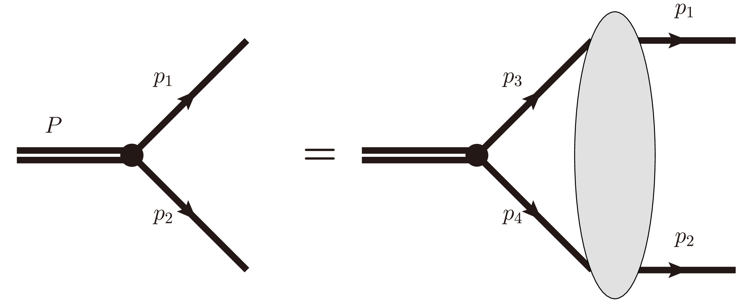
where $ P = (P_0,{\bf{0}})\equiv p_1+p_2 = p_3+p_4 $; $ p_{1,2,3,4} $ are the momenta of final and intermediate fermions, as shown in Fig. 1; $ E_{i}^{e}\equiv\sqrt{{\boldsymbol{p}}_i^2+m_e^2} $; $ E_{i}^{p}\equiv\sqrt{{\boldsymbol{p}}_i^2+m_p^2} $; $ {\boldsymbol{p}}_i $ are the three momenta of $ p_i $; $ m_{e,p} $ are the masses of the electron and proton; and $ \lambda, \mu $ are the indices related to the spinors. The interaction kernel $ \widetilde{K}_{\bar{\lambda}\lambda, \bar{\mu}\mu}({\boldsymbol{p}}_{1}, {\boldsymbol{p}}_{3}, P) $ is defined as

Figure 1.  Diagram for the BS equation.

where the spinors are chosen as

where $ \chi(+) = (1,0)^\dagger $ and $ \chi(-) = (0,1)^\dagger $. The kernel $ \bar{K}({\boldsymbol{p}}_{1}, {\boldsymbol{p}}_{3}, P) $ is defined as

where $ \tau_e\equiv m_e/(m_e+m_p) $, and $ K_{ {\rm{BS}}} $is the usual two-body BS irreducible kernel. Here, we directly make the assumption that the inverse $ [I-K_{ {\rm{BS}}}(G_0-\bar{G}_0)]^{-1} $ exists, and that $ \bar{K} $ can be expressed in a perturbative form as follows:

where

In the above expressions, $ S^{(e,p)}_{\rm full} $ are the full propagators of the electron and proton [10], respectively, and $ \Lambda_{\pm}^{a}({\boldsymbol{k}}) $ are

with $ E^{a}({\boldsymbol{k}})\equiv \sqrt{{\boldsymbol{k}}^2+m_a^2} $.

In the leading order of $ \alpha_e $, $ {\boldsymbol{p}}_{i}/m_{e,p} $, and $ m_e/m_p $, the interaction kernel $ \widetilde{K} $ can be chosen as

where

By utilizing this effective interaction kernel and expanding the equation in terms of momenta and bound energy, the effective Schrödinger-like equation Eq. (1) simplifies to the Schrödinger equation with the Coulomb potential. The contributions from interaction kernels involving higher orders of $ \alpha_e $, $ {\boldsymbol{p}}_{i}/m_{e,p} $, and $ m_e/m_p $ beyond $ \widetilde{K}^{(0)}({\boldsymbol{p}}_{1}, {\boldsymbol{p}}_{3}, P) $ can be estimated systematically using the bound-state perturbative theory, order by order. This approach can also be applied in NRQED, where the power counting and analytical calculations are more straightforward.

In the bound-state perturbative theory, the interaction kernels are expanded order by order in terms of $ {\boldsymbol{p}}_i/m_{e,p} $, and the corresponding matrix elements often exhibit divergences. To handle these divergences, regular methods are employed during the intermediate calculations. It is important to note that these divergences arise naturally owing to the slow decrease of the wave functions of the bound states with respect to momenta $ {\boldsymbol{p}}_i $, whereas the expansion of the interaction kernels in terms of momenta is not valid in the high momentum region.

In this study, we adopt a different approach by not expanding the interaction kernel $ \widetilde{K}({\boldsymbol{p}}_{1}, {\boldsymbol{p}}_{3}, P) $ in terms of $ {\boldsymbol{p}}_i/m_{e,p} $ and $ m_e/m_p $. Instead, we employ a numerical method to directly solve Eq. (1) using the leading-order $ \alpha_e $ expression of $ \widetilde{K}({\boldsymbol{p}}_{1}, {\boldsymbol{p}}_{3}, P) $.

In the leading order of $ \alpha_e $, only the OPE interaction contributes. As an approximation, we consider the proton to be a point-like particle in this study. Therefore, we have

and

where $ D_{\mu\nu}(p_1-p_3) $ refers to the propagator of the photon. In the Coulomb gauge, we have

and

with $ q = p_{1}-p_3 $, and $ j,k = 1,2,3 $. Here, $ q^0 = 0 $ because of the special choice of the momenta with $ p_{1}^{0} = p_{3}^{0} = \tau_e P_0 $.

After performing the necessary calculations, we obtain the following result:

where

and

with

By expanding the potential V in terms of $ {\boldsymbol{p}}_{i}/m_{e,p} $, it can be verified that the leading-order term corresponds to the Coulomb potential, while the next-leading-order terms correspond to the Breit potential. The higher-order terms correspond to the effective potential beyond the Breit potential. Similarly, the expansion results correspond to the amplitude in NRQED at the leading order of $ \alpha_e $, with higher orders of $ {\boldsymbol{p}}_i/m_{e,p} $.

Expanding $ H_p \equiv V + (E_1^{e}+E_1^{p}-m_e-m_p)(2\pi)^3\delta^3({\boldsymbol{p}}_1-{\boldsymbol{p}}_3) $ in terms of momenta yields the following results:

where

with

Here, $ H_p^{(4)} $ corresponds to the Breit potential in momentum space.

In perturbative bound-state theory, for a state $ | n,l,j,F \rangle $, labeled as $ nl_j^F $, where n is the principal quantum number, l corresponds to the orbital angular momentum of the electron, j corresponds to the sum of the spin and orbital angular momentum of the electron, and F corresponds to the total angular momentum, the energy contribution of hydrogen owing to the OPE interaction can be written as

where

Here, $ \alpha_e\equiv \dfrac{{\rm e}^2}{4\pi},\mu = \dfrac{m_em_p}{m_e+m_p} $, and Q is a projection operator on a subspace orthogonal to $ |n,l,j,F \rangle $.

The calculation of $ E_{n,i}^{(4)} $ can be performed directly, and the analytic results are expressed as

where

The calculation of $ E_n^{(6)} $ is somewhat complex [27−30], and there is a UV divergence in the middle matrix elements for the S wave, as explained above. In this study, we do not compare these results.

The wave function in Eq. (1) can be written as

This results in the following equation:

To compare with the results in Eq. (22), we also consider the state of the system as $ nl_{j}^{F} $. For $ F = j\pm\frac{1}{2} = l\pm1 $, we have the following form for $ \Phi_{\alpha,\beta}({\boldsymbol{p}}_3) $:

where $ F_z $ is taken as F, and only $ s_z^e $ and $ s_z^p $ need to be summed. When the effective potential V does not include spin-dependent terms, the above form of the wave function gives the same result as the following form:

We would also like to mention that the form of the wave functions expressed by Eq. (25) corresponds to the quantum numbers in non-relativistic quantum mechanics. When discussing states in QED, one can consider $ J^P $ as suitable quantum numbers to determine the most general form of the wave function $ \Phi_{\alpha,\beta} $ for solving the equation. In this case, effects such as mixing of the S and D waves naturally appear. However, in this study, we limit our discussion to the relativistic effects when considering the above form of the wave functions.

To calculate the energy contributions beyond the bound-state perturbative theory, we expand $ \Phi_{nlm}({\boldsymbol{p}}) $ as

where

where $ C $ is the Gegenbauer polynomial, $ \bar{p}\equiv a p $, and $ a = \dfrac{1}{\mu {\rm e}^2} $is the Bohr radius.

By choosing a specific value of $ n_{\rm max} $, one can calculate the following matrix:

where $ \Phi^{(0)}_{\alpha,\beta;i}({\boldsymbol{p}}_1) $ is simply $ \Phi_{\alpha,\beta}({\boldsymbol{p}}_1) $ in Eq. (25) after replacing $ \Phi_{nlm}({\boldsymbol{p}}_1) $ with $ \phi^{(0)}_{il}(|{\boldsymbol{p}}_1|)Y_{lm} $. The integration over the angles $ \Omega_{{\boldsymbol{p}}_1} $ and $ \Omega_{{\boldsymbol{p}}_3} $ can be performed analytically, while the integration over $ |{\boldsymbol{p}}_1| $ and $ |{\boldsymbol{p}}_3| $ can be performed numerically with high precision. After diagonalizing this matrix, the energy spectrum $ E_{n}\equiv P_{0,n}-m_e-m_p $ is obtained approximately.

We would like to highlight a significant difference between the method described above and the bound state perturbative theory. In the latter, non-relativistic potentials are utilized order by order. These non-relativistic potentials can lead to additional UV divergences in certain matrix elements, which are only canceled when all intermediate states are considered. In contrast, our calculation correctly accounts for the higher energy behavior of the effective potential, and there are no additional UV divergences; a finite $ n_{\rm max} $ can yield precise results. We elaborate on this property in detail in the next section.

In our numerical calculations, we set $ n_{\rm max} = 100 $, and the physical constants were set as $ m_e = 0.510998950 $ MeV, $ m_p = 938.27208816 $ MeV, and $ 1/\alpha_e = 137.035999084 $. The relative precision of the numerical calculation for each matrix element reached $ 10^{-20} $, ensuring that the absolute precision of the matrix elements was better than $ 10^{-18} $ eV. This guarantees the reliability of the numerical results. The numerical precision was also tested for the matrix elements involving the Coulomb and Breit potentials.

To compare the results with those obtained using the bound-state perturbative theory, we decompose the effective potential into three terms as follows:

where $ V_0 $ is spin-independent, $ V_1 $ depends only on the electron spin, and $ V_2 $ depends on the proton spin. We label the energy contributions corresponding to $ V_0,V_{0}+V_{1}, V_{0}+V_{1}+V_{2} $ as $ E_{n,0},E_{n,1},E_{n,2} $, respectively. The contributions beyond the Breit potential are expressed by the following quantities:

We present the numeric results for $ \Delta E_{n,i} $ in Tables 1, 2, and 3, respectively, where $ l = 0,1,2 $ or $ S,P,D $ waves, $ j = l+1/2 $, and $ F = l+1 $ are considered. For a more direct comparison, we also provide the contributions with specific orders as follows:

$n$	peV
	$\Delta E_{n,0}(S)$	$\Delta E_{n,0}(P)$	$\Delta E_{n,0}(D)$
$n=1$	−2349361	−	−
$n=2$	−289552	813	−
$n=3$	−85154	424	13
$n=4$	−35738	242	16
$n=5$	−18225	151	14

Table 1.  Numeric results for the energy corrections $\Delta E_{n,0}(l)$, where the unit is peV ($10^{-12}$ eV).

$n$	peV
	$\Delta E_{n,1}(S)$	$\Delta E_{n,1}(P)$	$\Delta E_{n,1}(D)$
$n=1$	−2349361	−	−
$n=2$	−289552	−44	−
$n=3$	−85154	50	3
$n=4$	−35738	48	6
$n=5$	−18225	37	6

Table 2.  Numeric results for the energy correction $\Delta E_{n,1}(l)$ with $j=l+1/2$, where the unit is peV ($10^{-12}$ eV).

$n$	peV
	$\Delta E_{n,2}(S)$	$\Delta E_{n,2}(P)$	$\Delta E_{n,2}(D)$
$n=1$	−2357360	−	−
$n=2$	−290555	−45	−
$n=3$	−85452	50	3
$n=4$	−35864	48	6
$n=5$	−18289	37	6

Table 3.  Numeric results for the energy correction $\Delta E_{n,2}(l)$ with $F=j+1/2=l+1$, where the unit is peV ($10^{-12}$ eV).

The results in Tables 1, 2, and 3 clearly demonstrate a notable property whereby the contributions in the S wave are significantly larger than those in the P and D waves.

In terms of magnitude, the contributions $ \Delta E_{n,0}(S) $ are approximately $ -\dfrac{\alpha_e^5\mu}{4.5n^3}\sim -\dfrac{30\alpha_e^6\mu}{n^3} $, which are larger than the contributions at the order of $ \dfrac{\alpha_e^6\mu}{n^3} $. The contributions $ \Delta E_{n,0}(P) $ are on the order of $ \dfrac{\alpha_e^6\mu}{20n^2} $. By contrast, the contributions $ \Delta E_{n,0}(D) $ weakly depend on $ n $ and are much smaller than $ \alpha_e^6\mu $.

The results for $ \Delta E_{n,1}(S) $ and $ \Delta E_{n,2}(S) $ are similar to those for $ \Delta E_{n,0}(S) $, indicating that the contributions from spin-independent terms are most significant for the S wave. This is expected, as the contributions from electron spin are zero for the S wave, and the contributions from proton spin are greatly suppressed.

The results for $ \Delta E_{n,1}(P) $ and $ \Delta E_{n,2}(P) $ are similar to each other and differ significantly from $ \Delta E_{n,0}(P) $. This indicates that in the P wave, the contributions from the electron spin are of the same order as the spin-independent contributions. The spin-dependent contributions in the D wave are similar to those in the P wave.

To illustrate the contributions more explicitly, we define the following terms:

These terms reflect the corrections to the fine structure and hyperfine structure beyond the Breit potential, respectively.

The numeric results for $ \Delta E_{n}^{fin} $ and $ \Delta E_{n}^{hyf} $ are presented in Tables 4 and 5, respectively. The numerical results in Table 4 indicate that the contributions to the fine structure beyond the Breit potential are approximately $ -\dfrac{\alpha_e^6\mu}{22n^2} $ in the P wave and $ -10 $ peV in the D wave. These values are much smaller compared to the contributions of $ -\dfrac{\alpha_e^6\mu}{n^2} $. The numeric results in Table 5 show that the contributions to the hyperfine structure beyond the Breit potential are approximately $ -\dfrac{200\alpha_e^6\mu}{n^3}\dfrac{m_e}{m_p} $ for the S wave, while the contributions are negligible for the P and D waves.

$n$	peV
	$\Delta E_{n}^{fin}(S)$	$\Delta E_{n}^{fin}(P)$	$\Delta E_{n}^{fin}(D)$
$n=1$	0	−	−
$n=2$	0	−857	−
$n=3$	0	−374	−10
$n=4$	0	−194	−10
$n=5$	0	−114	−8

Table 4.  Numeric results for the energy correction $\Delta E_{n}^{fin}(l)$ with $j=l+1/2$, where the unit is peV ($10^{-12}$ eV).

$n$	peV
	$\Delta E_{n}^{hyf}(S)$	$\Delta E_{n}^{hyf}(P)$	$\Delta E_{n}^{hyf}(D)$
$n=1$	−7999	−	−
$n=2$	−1003	$-0.66$	−
$n=3$	−298	$-0.27$	$-0.007$
$n=4$	−126	$-0.14$	$-0.007$
$n=5$	−65	$-0.08$	$-0.005$

Table 5.  Numeric results for the energy correction $\Delta E_{n}^{hyf}(l)$ with $F=l+1$, where the unit is peV ($10^{-12}$ eV).

To demonstrate the uncertainty arising from the approximation of finite $ n_{\text{max}} $, we plot $ \Delta E_{l+1,0}(l,n_{\rm max}) $ as a function of $ n_{\rm max} $ in Fig. 2. The results clearly indicate that the uncertainty is smaller than $ 0.5 $ peV when $ n_{\rm max}>60 $, suggesting that the approximation is reliable.

Figure 2.  (color online) Numeric results for $ \Delta E_{l+1,0}(l,n_{\text{max}}) $ vs. $ n_{\rm max} $ with $ l = 0,1 $ and 2, where the unit is peV ($ 10^{-12} $ eV).

In our calculations, we do not expand the OPE interaction kernel order by order in momenta; instead, we solve the effective Schrödinger-like equation using a numerical method. This approach enables us to include all contributions from ladder diagrams with the approximated propagator $ \bar{G}_0 $ and full photon propagator, while excluding the crossed diagrams. Consequently, the comparison of our results with those obtained from higher-order bound-state perturbation theory is not straightforward. To directly compare the pure relativistic contributions due to the OPE interaction by the two approaches at higher orders, one would need to separate the contributions in the bound-state perturbation theory based on the diagram types and momentum regions, and then compare them with our results. In the bound-state perturbation theory, the pure relativistic contributions are usually mixed with the same-order radiative corrections. Therefore, we only compare our results with $ E^{(2)}+E^{(4)} $.

In summary, the effective potential associated with the full OPE interaction in momentum space is expressed through eight scalar functions. The expansions of these scalar functions directly correspond to the $ ep\rightarrow ep $ amplitude in NRQED or the quasi-potential at order $ \alpha_e $ and any desired order of momenta. Our precise numerical calculations suggest that all relativistic contributions can be captured using this method. Extending these calculations to positronium, muonic hydrogen, and cases involving nuclear structure and radiative corrections would be interesting directions for future research.

H. Q. Z. would like to thank Zhi-Hui Guo, Xiao-Hai Liu, and Zhen-Xiang Zhong for their helpful suggestions and discussions.