Effective decay rates of nuclei in astrophysical environments

In nuclear astrophysics, the prediction of elemental abundance relies on incorporating nuclear reaction rates and decay rates into stellar models to simulate nucleosynthesis processes. This approach is fundamental for understanding the origin of elements in the universe. Nuclear β-decay plays a pivotal role at various stages of stellar evolution. Understanding nuclear decay rates in astrophysical environments is essential for unraveling the origins of elements in the universe. However, nuclear decay rates in stars can differ markedly from those observed on Earth.

Pioneering work by Cameron [1] demonstrated the importance of thermally populated excited states in enhancing decay rates. Specifically in stellar environments, nuclei are frequently excited by high-energy photons, leading to decay rates that differ significantly from those of ground states. Moreover, Bahcall [2] as well as Peterson and Bahcall [3] highlighted that elevated electron number density enhances electron-capture (EC) rates by supplying more high-energy electrons, while simultaneously suppressing $ \beta^- $ decay through Pauli blocking (occupied final electron states) [4]. Notably, in high-temperature (T$ > 1$ $ T_7 $($ 10^7 $ K)) and high-density (ρ$ > 10^3 $g/cm³) stellar interiors, elements undergo partial or complete ionization. As a result, the effective nuclear charge increases significantly, suppressing charge shielding effects. Furthermore, complete ionization eliminates bound-state electron capture (EC) due to the absence of orbital electrons. Most critically, ionization induced mass adjustments modify nuclear Q-values, enabling otherwise forbidden decays [5]. This effect is magnified for nuclei with laboratory measured β-decay Q-values that are small or marginally negative [6]. For example, the Q-value of $ \beta^- $decay for fully ionized ²⁰⁵Tl is 31.1(5) keV in the stellar interior, whereas the Q-value for its neutral atom is −50.6 keV under laboratory conditions.

Temperatures and densities can vary greatly in different nucleosynthesis environments. Therefore, stellar plasmas, where nucleosynthesis occurs, are not always fully ionized, and when thermodynamical conditions affect the ionization degree of the involved atoms, the β-decay process of their nuclei can also be strongly modified. Such an effect was first shown in the seminal work by Takahashi and Yokoi published in 1987 [7]; after 35 years, these values are still the most used in calculations of stellar and primordial nucleosynthesis. It is assumed that the initial nuclear states are in thermal equilibrium. The assumption of instantaneous thermal equilibrium may fail for nuclei exhibiting metastable isomers [7], such as ²⁶Al, and internal γ transitions from the isomer ($ 0^{+} $) to the ground state ($ 5^{+} $) are inhibited by the large spin difference. Here, equilibration between isomeric and ground states occurs indirectly via intermediate levels [8]. Ward and Fowler [8] proposed a generalized framework for multi-level equilibration. However, their model neglects the critical effects of ionization degree and electron number density, which dominate in high-temperature stellar plasmas.

This study established a unified computational framework for β-decay rates in astrophysical environments, explicitly integrating four critical parameters: temperature (T), electron number density ($ n_e $), ionization states, and nonthermal equilibrium corrections. The effective decay rates of ⁵⁹Fe, ⁷⁹Se, and ²⁰⁵Pb were calculated using the latest experimental data.

In stellar environments, nuclei are frequently excited by high-energy photons, leading to the population of low-lying excited states, as illustrated in Fig. 1. The evolution of the abundance between the excited states is described by the following equations [9]:

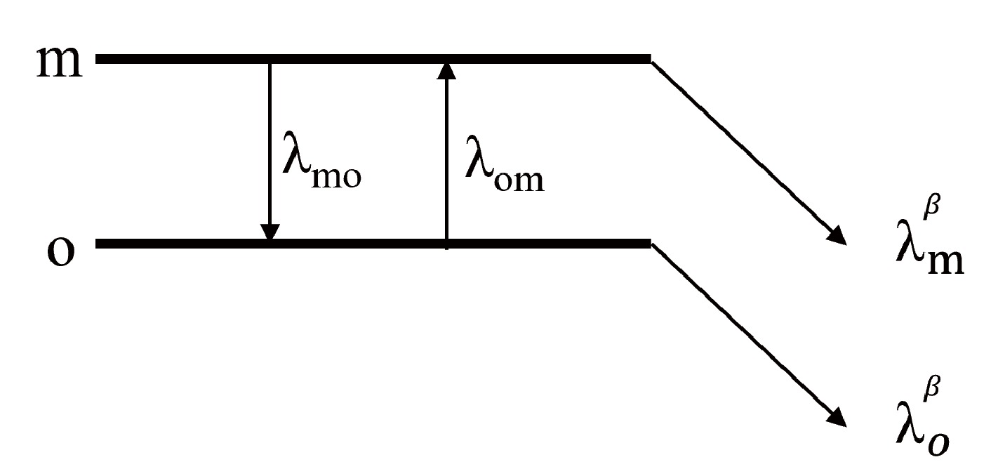
Figure 1.  Internal equilibration of a single excited state and the ground state of a nucleus.

The subscripts m and o indicate the excited and ground states, respectively. n is the abundance of the level. $ \lambda^{\beta}_m $ represents the β-decay rate of level m. $ \lambda_{mo} $represents the γ transition from level m to level o, which consists of spontaneous transitions and is stimulated by photons; it is expressed as

where $ \lambda^s_{mo} $ represents the spontaneous γ transition from level o to level m. T is temperature, $ k_B $ is the Boltzmann constant, and E is the energy of the nuclear level. $ \lambda_{om} $ represents the induced transition from level o to level m and is expressed as

where G is the partition function of nuclear level. For the case of internal equilibration, the abundance ratio of the two levels is given by

The effective decay rate λ is derived from the weighted average of the β-decay rates at different nuclear levels [7, 10]:

where the subscript K represents the nuclear level. $ P_K $ is the layout probability at thermal equilibrium. $ \lambda_K $ and $ E_K $ are the decay rate and energy, respectively. T is temperature.

In some cases, internal γ transitions from the isomer to the ground state are inhibited by the large spin difference, necessitating equilibration through an intermediate state, as illustrated in Fig. 2. The evolution of the abundance between the three levels for the nuclei is expressed as

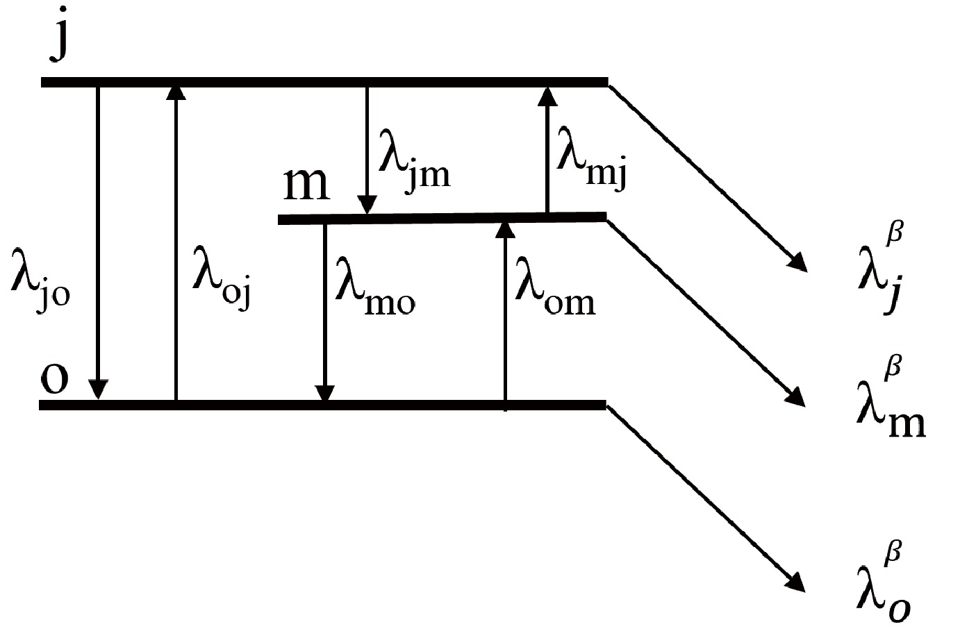
Figure 2.  Internal equilibration of a three-level nuclear system.

Ward and Fowler [8] provided general numerical calculations for this case. The rates of change of the abundances n of the nuclear levels can be writen by the coupled set of first order differential equations in matrix form as

where T is the β-decay and internal electromagnetic transition matrix [8] that follows from Eqs. (7)–(9), and

The general solution to this equation is of the form

where $ N_i $ and $ -\lambda_i $ are the eigenvectors and eigenvalues of T, respectively. By definition, the effective decay rate λ is expressed as

At the temperature of interest, for a sufficiently long time, if $ \lambda_3\ll\lambda_2 $ and $ \lambda_3\ll\lambda_1 $, the effective decay rate $ \lambda\approx\lambda_3 $.

Meanwhile, in the stellar environment, the nuclei may have different ionizations, such as bare nuclei, incompletely ionized atoms, and neutral atoms. $ \lambda_K $ is derived from the weighted average of decay rates at different ionization as follows [7]:

where the subscripts r and $ r+1 $ represent r-times and $ r+1 $-times ionized, respectively. $ N_r $ and $ P_r $ are the abundance and probability of the ion, respectively. The ionization probability of atoms in the stellar environment can be obtained from the Saha ionization equation [11]:

where $ b_r $ is the partition function of the r-times ionized atom, h is Planck's constant, and $ I_r $ is the ionization potential. In addition, electrons in an atom or ion can also be thermally excited in the same way as nucleons. $ \lambda_{K,r} $ is given by the following equation [7]:

where the subscript k is the level of the atom or ion. g is the partition function of the ion. $ \lambda_{K,r,k} $ is given by the following equation [7]:

where m=a, 1nu, 1u, and 2u represent allowed, non-unique first-forbidden, unique first-forbidden, and unique second-forbidden transitions, respectively. $ ft $ is the comparative half-life. For free electrons (positrons) to be emitted or captured, $ f_m $ is the phase space integral, given by [4, 12−14]

where W is the total, rest mass, and kinetic energy of the electron or positron in units of $ m_ec^2 $. Z is the proton number of the parent nucleus. $ Q_{ij} $ is the decay energy between the initial state of the parent i and final state of the daughter j in units of $ m_ec^2 $. $ W_{\mathrm{min}} $ is the lowest energy of the electron (positron) in the β-decay in units of $ m_ec^2 $:

$ F(Z,W) $ is the Fermi function [14−17]:

where

and

where α$ \approx \dfrac{1}{137} $ is the fine structure constant, Γ is the gamma function, and R is the nuclear radius in units of $ \hbar/mc $. $ S_m(Z,W) $ are the spectral shape factors [13, 15, 16]:

where $ W_v $ is the neutrino energy in units of $ mec^2 $. $ L_0 $, $ L_1 $, and $ L_2 $ are certain combinations of electron radial wave functions evaluated at an appropriately chosen nuclear radius R [13, 15, 16, 18]:

and

The last two terms of the phase space integal $ f_m $ are related to the electron, positron, and neutrino distributions. $ G_e $, $ G_p $, and $ G_v $are the Fermi–Dirac distribution functions of the electron, positron, and neutrino:

where $ E_e $, $ E_p $, and $ E_v $are the energies of the electron, positron, and neutrino in units of MeV, respectively. $ U_F $ is the Fermi energy of the electrons in units of MeV. The relation between Fermi energy and electron number density is given by [4, 13]

The chemical potential of the electron for given values $ \rho Y_e $ and T can be obtained by iterating Eqs. (31), (32), and (34).

For the bound-state $ \beta^- $ decay and bound-state (orbital) e^- capture processes, $ f_m $ is the lepton phase volume part, given by [17, 19]

where $ \sigma_x $ describes the vacancy (for bound-state $ \beta^- $ decays) or occupancy (for orbital e^- captures) of the electron orbit x and lies between zero and unity. [$ g_x $ or $ f_x $] is understood to be the larger component of the electron radial wave functions evaluated at nuclear radius R, which can be obtained by RADIAL with self-consistent method [20]. Here, $ S_{(m)x} $ are the spectral shape factors, given by [17, 19]

Having established the methodology for calculating the effective decay rates, we now present the results obtained under various astrophysical conditions.

In $ \beta^{+} $-decays, contributions from continuum and orbital electron capture processes are included, while in $ \beta^{-} $-decays, those from the bound state $ \beta^{-} $ processes are taken into account.

The nucleosynthesis of the observable long-lived radioactive nuclides ²⁶Al ($ T_{1/2}= $0.717 Myr) and ⁶⁰Fe ($ T_{1/2}= $2.26 Myr) is an important constraint on stellar models [21]. The abundances inferred from γ-ray astronomy may have important implications for rotationally induced mixing, convection theory, mass loss theory, the initial mass function for massive stars, and the distribution of metals in the Galaxy [22].

However, the predicted yield ratio ⁶⁰Fe/²⁶Al is larger than the experimental value [21]. Studies have shown that the main source of theoretical prediction uncertainty is the reaction cross section of the generation and destruction of these isotopes. The Log $ ft $ values of ²⁶Al and ⁵⁹Fe are listed in Tables 1 and 2, respectively. Therefore, to constrain the yield ratio ⁶⁰Fe/²⁶Al, it is necessary to calculate the decay rate. Internal γ transitions from the isomer ($ 0^{+} $) to the ground state ($ 5^{+} $) of ²⁶Al are inhibited by the large spin difference. Thus, thermal equilibrium cannot be established between the ground state and first excited state, but it can be achieved through an intermediate state [8, 9, 23]. The γ decay rates of ²⁶Al (internal) are listed in Table 3.

Transitions	Log $ft$
g.s.$\rightarrow $1.809 MeV	14.18
g.s.$\rightarrow $2.938 MeV	13.35
0.228 MeV$\rightarrow $g.s.	3.48
0.417 MeV$\rightarrow $1.809 MeV	3.63
0.417 MeV$\rightarrow $2.938 MeV	4.66
1.058 MeV$\rightarrow $g.s. MeV	4.01
1.058 MeV$\rightarrow $1.809 MeV	3.36
1.058 MeV$\rightarrow $2.938 MeV	4.63

Table 1.  Log $ft$ values for the decay of ²⁶Al$\rightarrow $²⁶Mg [4].

Transitions	Log $ft$
g.s.$\rightarrow $1.099 MeV	6.7 [24]
g.s.$\rightarrow $1.292 MeV	5.98 [24]
0.473 MeV$\rightarrow $g.s.	5.41 [21]
0.571 MeV$\rightarrow $g.s.	5.55 [21]

Table 2.  Log $ft$ values for the decay of ⁵⁹Fe$\rightarrow $⁵⁹Co.

Transitions	Multipolarity	$\lambda(s^{-1})$
0.417 MeV$\rightarrow $g.s.	E2	6.88×108
0.417 MeV$\rightarrow $228 MeV	M3	0.062
1.058 MeV$\rightarrow $417 Mev	E2	7.24×108

Table 3.  Electromagnetic transition rates of ²⁶Al [23].

In this case, the method of Runkle [23] is used to describe the internal behavior of the system (equilibration) at high temperatures. The evolution of the clusters can be written as

where the subscripts o, m, 2, and 3 refer to the ground state, isomer, 417 keV, and 1058 keV states, respectively. The β decay rates $ \lambda^\beta $ for each level are obtained by Eqs. (15)–(36), which are different from those of Runkle [9, 23] in that the effects of electron number density, chemical potential, and ionization are ignored. The factors $ c_{ij} $ are the thermal equilibrium abundance $ c_{ij} $ ratios

This can be recast as a matrix equation

where T is the transition matrix that follows from Eqs. (37) and (38), and

The smaller eigenvalues λ of T are related to the effective decay rate of ²⁶Al [23].

The effective decay rate of ²⁶Al is depicted in Fig. 3, illustrating the significant impacts of temperature and electron number density on its decay behavior. As the electron number density increases, the chemical potential of electrons rises, leading to an enhancement in the electron capture decay rate. The electron density dependence of positron emission is negligible in most cases of interest. With an increase in temperature, the decay rate of electron capture increases significantly owing to the increase in the contribution of excited states. At temperatures between 0.2 $ T_9 $ and 0.4 $ T_9 $, the decay rate exhibits minimal dependence on the electron number density. This is because the thermal layout rate from ground state population to the first excited state is smaller than the β-decay rate of the first excited state at lower temperatures. In this case, the actual decay rate of the first excited state will be determined by its thermal layout rate, which is independent of electron number density. As the temperature continues to increase, the thermal equilibrium rate begins to exceed the β-decay rate. At this point, the interior of the nucleus can reach thermal equilibrium so that the effective decay rate of the nucleus is not restricted by the thermal layout rate. When incomplete thermal equilibrium is considered, the effective decay rate of the nuclei is smaller than the thermal equilibrium because of the restriction of the thermal layout rate at lower temperatures. Our calculations show that the effective decay rate is amplified by a factor of $ 10^{10} $ when the effects of the celestial environment are taken into account. This has a significant effect on the production of ²⁶Al in the star.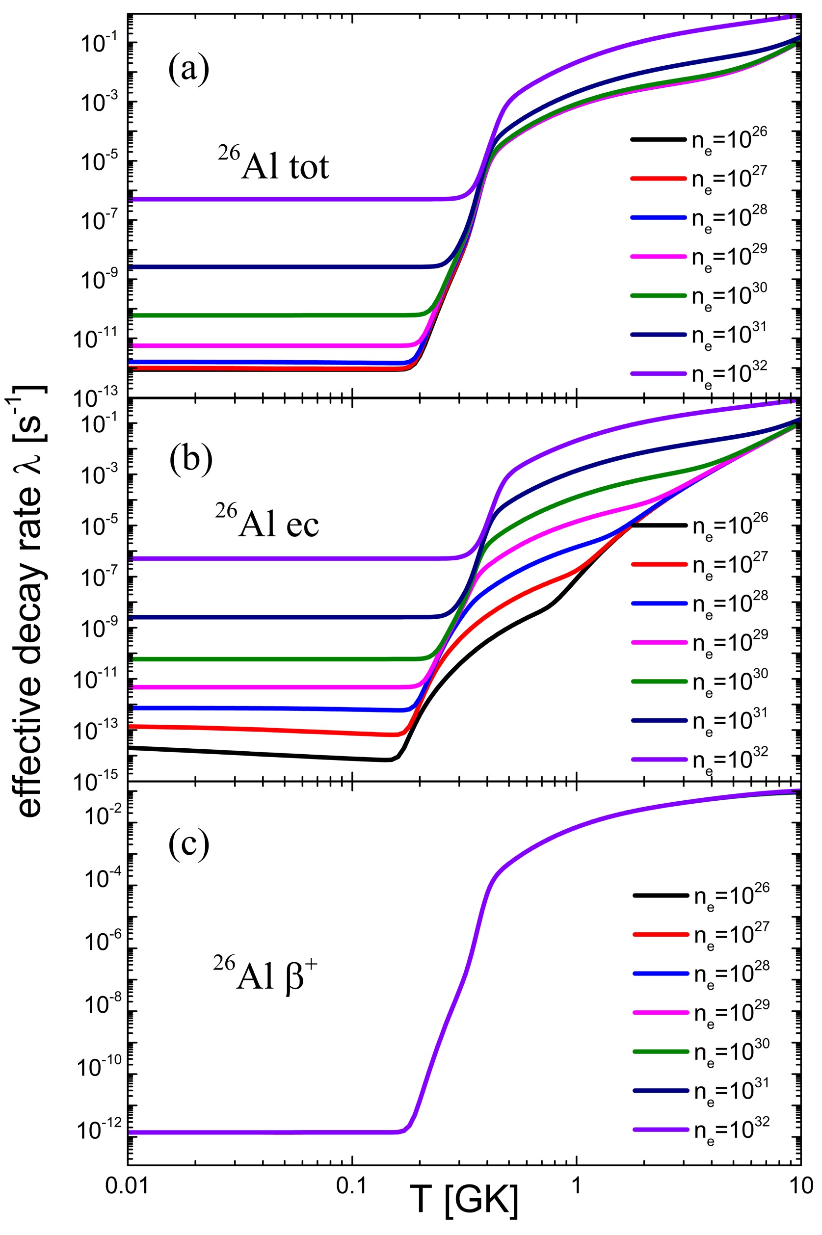

Figure 3.  (color online) Effective decay rate of ²⁶Al as a function of T and $n_e$. (a) Effective total decay rate $ \lambda_{\mathrm{tot}} $ of ²⁶Al as a function of T and $n_e$. (b) Effective electron capture decay rate $\lambda_{ec}$ of ²⁶Al as a function of T and $n_e$. (c) Effective decay rate $\lambda_{\beta^+}$ of ²⁶Al as a function of T and $n_e$.

As mentioned above, to constrain the yield ratio ⁶⁰Fe/²⁶Al, Gao et al. [21] measured the $ B(GT) $ of the low excited state of ⁵⁹Fe to calculate the effective $ \beta^- $-decay rates and showed that the ⁶⁰Fe production yield of an 18 solar mass star by ⁵⁹Fe(n, γ) reaction is decreased significantly by 40%. However, the effect of electron number density and ionization was ignored in their research. To study the yield of ⁶⁰Fe, it is necessary to consider the environmental impact more comprehensively.

The effective decay rate of ⁵⁹Fe is calculated by considering the influences of temperature, electron number density, and ionization, as shown in Fig. 4. With an increase in temperature, the decay rate of ⁵⁹Fe increases by up to 1000 times. In contrast, the decay rates decrease with increasing environmental electron density. When the electron number density is $ 10^{30} $, the effective decay rate is reduced by a factor of 10. When the electron number density $ n_e $ is greater than $ 10^{29} $, the effective decay rate of ⁵⁹Fe is significantly reduced. This leads to an increase in the production of ⁶⁰Fe in the stellar interior.

Figure 4.  (color online) Effective $\beta^-$ decay rate $\lambda_{\beta^-}$ of ⁵⁹Fe as a function of T and $n_e$.

⁷⁹Se is a branching point in the slow neutron capture process (s-process), with relevant implications in nucleosynthesis and stellar models. The products of the s-process nucleosynthesis after ⁷⁹Se are the s-only isotopes ^80,82Kr, whose solar system abundances are accurately known. The Log ft value of ⁷⁹Se is listed in Table 4. The ground state half-life of ⁷⁹Se is 0.327 My, and its first excited state is 2 h. Therefore, the half-life of ⁷⁹Se is sensitive to the temperature of the stellar interior. This information, in conjunction with the decay rate of ⁷⁹Se, allows one to extract reliable conditions for temperature and neutron and electron number densities. The effective decay rate of ⁷⁹Se was given by Takahashi and Yokoi in 1987 [7]. However, the ground state of ⁷⁹Se was missing from their calculations, and the decay rates of the first excited and ground states were updated.

Transitions	Log $ft$
g.s.$\rightarrow $g.s.	10.8
0.096 MeV$\rightarrow $g.s.	4.7 [25]

Table 4.  Log $ft$ values for the decay of ⁷⁹Se$\rightarrow $⁷⁹Br.

The effective decay rate of ⁷⁹Se was obtained using the latest data, as shown in Fig. 5. The effective decay rate of ⁷⁹Se is very sensitive to temperature. As the temperature rises, the effective decay rate of ⁷⁹Se increases by five orders of magnitude. In contrast, the decay rates decrease with increasing environmental electron density. In summary, the effective decay rate in the environment of interest is significantly greater than that on earth. This results in a lower yield ratio of ⁸²Kr/⁸⁰Kr. This is of great significance to the study of the s-process.

Figure 5.  (color online) Effective $\beta^-$ decay rate $\lambda_{\beta^-}$ of ⁷⁹Se as a function of T and $n_e$.

As a unique pure s-process nucleus, ²⁰⁵Pb can be used not only as a unique nucleosynthesis tracer but also as a ²⁰⁵Pb-²⁰⁵Tl clock to time the evolution of elements [26]. In conclusion, ²⁰⁵Pb provides a unique opportunity to study s-process nucleosynthesis, which has important implications for the study of cosmic evolution and solar system formation. This was analyzed by Dong et al. [27], and the origin of ²⁰⁵Pb in the solar system was investigated. At the temperature of interest, the layout probability $ P_K $ of the first excited state of ²⁰⁵Pb is relatively large, as shown in Fig. 6. The decay rate of the first excited state (2.32 keV) is much greater than that of the ground state for this isotope. Thus, the effective decay rate of ²⁰⁵Pb is very sensitive to temperature. Meanwhile, the higher electron number density can greatly increase the electron capture rate in the stellar interior. To obtain the yield of ²⁰⁵Pb, it becomes crucial to calculate the effective decay rate of ²⁰⁵Pb. In 2024, Leckenby [28] measured the bound-state $ \beta^- $ decay of ²⁰⁵Tl to determine the Log $ ft $ value of the first excited state of ²⁰⁵Pb, which further constrained the uncertainty brought by the input.

Figure 6.  (color online) Thermally populated probability $P_K$ and ionization probability $P_r$ as functions of T and $n_e$. (a) Thermally populated probability $P_K$ of ²⁰⁵Pb as a function of T and $n_e$. (b) Ionization probability $P_r$ of ²⁰⁵Pb as a function of T.

The ionization probability $ P_r $ of ²⁰⁵Pb obtained using the Saha equation varies with temperature and density, as shown in Fig. 6. The ionization probabilities of ²⁰⁵Pb⁸²⁺ and ²⁰⁵Pb⁷⁹⁺ in different environments are shown. In the celestial environment of interest, ²⁰⁵Pb⁸²⁺ is the main component, in addition to a large number of highly ionized states. When the temperature is$ 0.1\ T_9-0.3\ T_9 $, there is a large amount of highly ionized ²⁰⁵Pb. In this case, orbital electron capture significantly increases the decay rate.

The latest data in Table 5 were used to calculate the effective decay rate of ²⁰⁵Pb, as shown in Fig. 7. As the temperature increases, the decay rate of ²⁰⁵Pb increases by a factor of $ 10^8 $. With an increase in temperature, the thermal distribution probability of the first excited state of 2.32 keV increases, and the decay rate becomes faster. The decay rate of ²⁰⁵Pb from temperatures of 0.002 to 0.05 $ T_8 $ are enhanced significantly by the thermal population of the first excited state. Above 0.05 $ T_8 $, the rate decreases owing to increasing ionization, which reduces the available bound electrons to be captured. The electron capture rate increases with increasing electron number density. In summary, the decay rate of ²⁰⁵Pb is sensitive to temperature and electron density. To study the abundance ratio of ²⁰⁵Pb/²⁰⁵Tl in the early solar system, it is necessary to consider the influence of the environment on the decay.

Transitions	Log $ft$
g.s.$\rightarrow $g.s.	12 [7]
0.00232 MeV$\rightarrow $g.s.	5.91 [27]
0.262 MeV$\rightarrow $g.s.	6.5 [7]

Table 5.  Log $ft$ values for the decay of ²⁰⁵Pb$\rightarrow $²⁰⁵Tl.

Figure 7.  (color online) Effective electron capture decay rate $ \lambda_{ec}$ of ²⁰⁵Pb as a function of temperature and electron number density.

In this study, we developed a comprehensive framework for calculating the effective decay rates of nuclei in astrophysical environments, incorporating the effects of temperature, electron number density, ionization, and nonthermal equilibrium. Using ²⁶Al as a case study, we addressed the challenge of incomplete thermal equilibrium due to large spin differences in internal γ-transitions between the isomer ($ 0^+ $) and ground state ($ 5^+ $). This extends the work of Takahashi and Yokoi [7] by providing a more nuanced understanding of nuclear decay in stellar environments. We also calculated the effective decay rates of ⁵⁹Fe, ⁷⁹Se, and ²⁰⁵Pb using the latest experimental data. Our results demonstrate that these decay rates vary significantly under the influence of astrophysical conditions, with particular sensitivity to temperature and electron density.

Notably, we found that the inclusion of electron number density in the decay rate calculation for ⁵⁹Fe, a factor overlooked by Gao [21], provides a more accurate representation of its astrophysical behavior. These findings have important implications for nucleosynthesis models. For instance, the yield ratio of ⁶⁰Fe/²⁶Al is significantly altered when environmental effects are considered. Furthermore, our results highlight the sensitivity of branching ratios in the s-process to astrophysical conditions, offering new insights into elemental abundance patterns.

In conclusion, our study underscores the importance of considering astrophysical environmental effects on nuclear decay rates, providing new insights into the origin of elements and constructing astrophysical nucleosynthesis. Future studies should extend this framework to other nuclei and explore additional environmental factors, such as magnetic fields and nonthermal equilibrium. Such studies will further refine our understanding of stellar evolution and the origin of elements in the universe.