Bayesian-optimized CatBoost for Ground-State Nuclear Charge-Radius Prediction

Nuclear charge radius ($ R_c $) is one of the most fundamental features of atomic nuclei and has been extensively investigated in nuclear physics [1]. It not only provides insights into the charge distribution within the nucleus and the overall nuclear shape but also the nuclear stability and behavior [2]. Ford et al. [3] emphasized the importance of nuclear charge radius in understanding nuclear shape and behavior. There are a number of experimental techniques to calculate charge radii, some of which have been in use since the mid-20th century. For example, one of the precise experimental techniques is electron scattering experiments for the determination of charge distribution of nuclei, or more specifically, electron scattering experiments of ⁶Li, ⁷Li, ¹²C, and ¹⁶O [4, 5]. Muonic atom spectroscopy and Kα X-ray isotope shift (KIS) are also being extensively used [6]. However, limitations in experimental techniques restrict their application to specific regions of the nuclear chart.

For this reason, a wide variety of nuclear models have also been developed, that can analyze ground state properties, including $ R_c $, with much greater accuracy. Macroscopic models, including the liquid drop model [7, 8] and the Garvey-Kelson relation [9] are the simplest approaches that provide preliminary insights into nuclear structure and its properties. For better predictions, phenomena like isospin dependence and shell effects have also been incorporated [10]. Microscopic models further enhance theoretical accuracy by delving into the nucleus at the nucleon level, focusing on individual interactions between protons and neutrons. The Skyrme-Hartree-Fock-Bogoliubov (HFB) models use the Skyrme interaction to model nucleon-nucleon forces, approximate the average potential experienced by each nucleon by using Hartree-Fock approximation, and handle pairing correlations by Bogoliubov transformation for accurate calculations [11, 12]. The relativistic effects on Skyrme-Hartree-Fock are studied in the RMF model [13]. Apart from these approaches, empirical formulae have also been derived by capturing the local relations, for example, $ \delta R $, i.e., the charge radii difference of two isotopes of a single element [14]. Advanced mean field models, e.g., deformed relativistic Hartree-Bogoliubov, offer a further deep description by adding properties like deformation and superfluidity [15−17]. Furthermore, ab initio no-core shell models consider direct interaction of nucleons without core approximations [18, 19]. Lastly, the Weizsäcker-Skyrme (WS*) model, which integrates both microscopic and macroscopic parameters for a better description of nuclear properties of exotic as well as stable nuclei [10].

Machine learning (ML) and deep learning (DL) offer high potential in their application to both theoretical and experimental nuclear physics [20]. For example, prediction of nuclear mass using support vector regressor and Gaussian process regressor shows good predictive capabilities both within and beyond the training set [21]. Application of machine learning algorithms over AME2020 data [22, 23], where ML models outperformed the semi-empirical Bethe-Weisäker formula [24]. Similarly, the impact parameter in heavy-ion collisions is determined by utilizing neural networks (NN) [25]. Predictive modeling of ground state energies of even-even nuclei by using ANNs over a theoretical dataset calculated using the Hartree-Fock-Bogoliubov (HFB) model [26]. The study of unstable nuclei relies heavily on α decay. An approach integrating the sophisticated α-decay model with a Bayesian neural network (BNN) is employed to enhance the prediction accuracy of α-decay half-lives. According to global and extrapolated analyses, model-based predictions of α decay can be more effectively described by the BNN approach [27]. The extreme gradient Boosting (XGBoost) framework is used to study the α-decay energy and half-life of superheavy nuclei, which are optimized using Bayesian hyperparameters. By incorporating key nuclear structural features, including mass number, proton-to-neutron ratio, magic number proximity, and angular momentum transfer, the optimized model captures essential physical mechanisms governing α-decay [28]. On the basis of WKB barrier penetrability, an improved formula considering the deformation effect for the α-decay half-lives is proposed. The improved empirical formula and XGBoost models were used to predict the α-decay half-lives of nuclei with Z = 117,118,119, and 120. You et al. [29], combined the empirical formulas with ML techniques to explore the effect of nuclear deformation on α decay half-lives, enhancing predictive performance within deformed regions. The α-decay energies and half-lives have also been studied using Gaussian process algorithm [30].

The recent and most comprehensive exploration of modern machine learning models in charge radii predictions, Bayram et al [31], showed high potential of both modern tree-based algorithms (XgBoost, Cubist) along with conventional machine learning. These models have a relatively low RMSE (0.03992-0.0119) fm. Jalili et al. [32] have extensively explored the Support Vector Regression (SVR) over a diverse range of Z and also pointed out the impact of including A as a feature on the model performance. Their most prominent contribution includes the novel application of RBF (Radial Basis Function) with SVR, a decrease in RMSE from 0.045 fm to 0.016 fm for over 1000 isotopes, as well as improved extrapolation ability of the model. Wu et al. [33] applied feed-forward networks with Z, N, and $ B(E2) $ inputs to capture magic-number kinks and study symmetry-energy links. Utama et al. [34] bridged Bayesian neural networks with density functional theory to substantially reduce prediction errors by three times. Ma et al. [35] used naive Bayes classifiers to refine HFB and semi-empirical radii, with notable gains in terms of accuracy. Dong et al. [36] reduced errors significantly by combining Bayesian networks with the NP formula, and Dong et al. [37] later included physics-driven features to overcome overfitting. Recently, Jian et al. [38] implemented a continuous Bayesian probability (CBP) estimator and Bayesian model averaging (BMA) to enhance the predictions of charge radii from sophisticated theoretical nuclear structure models. They combined the CBP estimator and BMA to refine charge radii predictions from the HFB, RHB, and semi-empirical liquid-drop model. Their method pushed the standard deviation in predictions of $ R_C $ below 0.02 fm, demonstrating a strong potential for CBP and BMA in accurate predictions of nuclear charge radii.

Despite the theoretical and machine-learning studies being very broad, two prominent gaps persist. First, global models such as RHB reproduce broad charge-radius trends but fail to capture fine features at the isotopic chain level such as odd-even staggering and exotic-isotope kinks across the nuclear chart. Second, ML approaches (ANNs, Bayesian NNs, SVR) achieve competitive RMSEs but remain constrained by limited data and imbalanced experimental data, narrow feature sets, and a lack of interpretability. Moreover, most of the machine learning studies are limited to $ A\ge40 $ and $ Z\ge20 $. To the best of our knowledge, no work has leveraged CatBoost's ordered boosting with Optuna-TPE optimization, combined complementary experimental datasets and RHB-based theoretical features of PC-X data, and used SHAP analysis to provide feature-level insights both globally and at the chain level around N=50.

We present, the utlizations of CatBoost regression for predicting $ R_C $ in this work. The model is trained on merged and processed data extracted from three data tables: (Li et al. [39], Angeli et al. [40], and PC-X [41]. They systematically pushed our study range to $ A\ge17 $ and $ Z\ge8 $ below the previously reported range, i.e., $ A\ge40 $ and $ Z\ge20 $. For the best possible performance, the hyperparameters were efficiently searched with Optuna’s TPE sampler, and the model's interpretation was conducted with SHAP analysis. The Kr and Sr chains are reproduced to assess the model's ability to capture the characteristic “kink” at $ N=50 $ and odd-even staggering effects. We demonstrate that our approach outperforms the theoretical model (Skyrme-Hartree-Fock-Bogoliubov model) and established ML techniques in rigorously cross-validated tests. Our study's main contribution is better predictive performance by the first implementation of CatBoost, which is systematically combined with Optuna-driven Bayesian hyperparameter adjustment.

The structure of the paper is organized as follows. Section 2 presents a quick overview of the theoretical background of the CatBoost algorithm, Optuna’s Bayesian optimization with TPE sampler, SHAP values, and the RHB-derived physics features. Section 3) describes dataset merging and preprocessing, feature selection, hyperparameter tuning, and the model evaluation protocol. Section 4 reports cross-validation and hold-out performance, comparative benchmarking, optimization history, SHAP insights, and isotopic-chain kink reproduction. Section 5 concludes the main findings of this work and outlines directions for future research.

The CatBoost algorithm works on the gradient boosting framework using functional gradient descent to iteratively improve an ensemble predictor [42]. After every iteration m, the current approximation $ F_{m-1} $ is updated simply as

where $ p_{m} $ shows the step size and $ h(x;a_{m}) $ is a chosen binary decision tree parameterized by $ a_{m} $, which is used to estimate the negative gradient of the loss over the training data [42]. Each tree segregates the feature space into disjoint regions and fits constant values on the leaves, which builds its structure greedily to minimize residual error.

CatBoost fits gradient-boosted decision trees using a second-order expansion of a regularized loss [43], which is itself an implementation of Prokhorenkova et al. [42] and the original gradient boosting framework of Friedman [44] on the CatBoost model. At iteration t, the new tree $ w_t $ is chosen to minimize

where $ g_{i,t} = \partial_{W_{t-1}} \ell\bigl(y_i, W_{t-1}({x}_i)\bigr) $, $ h_{i,t} = \partial^2_{W_{t-1}} \ell\bigl(y_i, W_{t-1}({x}_i)\bigr) $ and $ u(w_t) $ denotes a regularization term to penalize the complexity of the tree. The distinct and powerful feature of CatBoost is ordered boosting. The standard gradient boosting approaches, such as XGBoost, LightGBM, and AdaBoost [45−47], are prone to overfitting on small or skewed datasets. These models are prone to overfitting the training set by learning from their residuals. This issue is addressed in the CatBoost using ordered boosting. Rather than building each tree using the entire training data, ordered boosting draws on progressively larger prefixes of data. For each new split, only previous observations (not those that are being split) are used to calculate gradients, preserving unbiasedness and independence (for further details, see [43]). CatBoost’s ability to perform unbiased ordered boosting and effective categorical feature handling makes it faster to train and improves its generalization ability compared to other boosting models.

Hyperparameter tuning is very crucial for achieving high model accuracy, but all the possible configurations can be extremely expensive since each combination of parameters requires full model training and validation. To address time and cost issues, we apply Optuna's Bayesian framework [48], that utilizes past trial results to direct subsequent search and lower the total number of evaluations. Hyperparameter tuning is formulated as

where $ x\in{\cal{X}} $ denotes a hyperparameter configuration and $ f(x) $ is the K-fold cross-validated loss. Optuna [48] constructs the search space dynamically within the objective using calls and allows conditional and hierarchical parameter definitions. It employs the tree-structured parzen estimator (TPE) sampler [49], which models two densities.

where $ \ell(x) $ is the density formed by the observations $ \{x^{(i)}\} $ with $ f(x^{(i)})<y^* $, and $ g(x) $ is formed by the remaining observations. The TPE algorithm depends on $ y^* $ to the quantile γ of the observed y-values, so that $ P(y<y^*)=\gamma $. New potential best combinations of hyperparameters are then drawn by maximizing the ratio $ \ell(x)/g(x) $, focusing the search only on the promising regions of the hyperparameter space. This complete package of dynamic search-space definition, Bayesian TPE sampling, and effective metadata storage provides efficient exploration of complex, high-dimensional hyperparameter space in a very short time and reduced computational cost.

SHAP (SHapley Additive exPlanations) [50] is a technique based on game theory and used to interpret the output of machine learning models by determining the contribution of each feature to the model's performance. SHAP values use Lloyd Shapley’s original cooperative game theoretic solution [51] to feature attribution in machine learning. The explanation model is given by a linear function of binary variables

uniquely satisfying the axioms of local consistency, accuracy, and missingness [50]. Then KernelSHAP approximates $ \{\phi_i\} $ using a single weighted regression; on the other hand, TreeSHAP calculates them exactly for tree ensembles in polynomial time [52].

In the present analysis, we employed the physics-driven features computed by [41] using the relativistic Hartree-Bogoliubov framework with separable pairing force incorporating the latest PC-X parametrization. The nonlinear point-coupling PC-X functional within the covariant density functional theory of nuclear structure provides a self-consistent description of bulk saturation, shell effects, and pairing effects. Instead of recomputing theoretical features, we utilized the S_n, S_2n, and BE directly from Ref. [41]. The reason behind our choice of features computed using PC-X functional was the large data volume, i.e., 9162 nuclei (ensuring BE values for virtually all of our experimental entries), and its demonstrated high fidelity in reproducing the experimental ground state properties, including BE and nuclear charge radii across the nuclear chart. These properties make it a reliable physics-driven feature source, encoding saturation properties, symmetry-energy effects, shell-closure behavior, and pairing correlations, laying the theoretical foundation for our CatBoost model.

This study makes use of three state-of-the-art datasets [39−41] to build this CatBoost model of nuclear charge radii. The first data source is [40] updated compilation of experimental charge radii, which contains experimentally measured charge radii of 909 isotopes ranging from hydrogen (Z = 1) to curium (Z = 96). The second data source [10] contains 257 samples of nuclear charge radii from beryllium (Z = 4) to radium (Z = 88), where 236 of them were measured using laser spectroscopy. The third data source is theoretical ground state properties of 9162 isotopes calculated using the relativistic Hartree-Bogoliubov framework with separable pairing forces along with the latest point coupling density functional PC-X [41]. First, we integrated the Angeli & Marinova’s with the latest data table compiled by Li, Luo & Wang. In the case of clashes, i.e., repetition of the charge radius of a single isotope in both datasets, we retained the latest charge radius compiled by Li, Luo, and Wang. This integrated dataset was then introduced with new columns of theoretical ground state properties from the 3rd dataset. A, N, and Z were used as identifiers for adding new features from the theoretical dataset. After the integration, Tukey’s “1.5 × IQR” rule [53] was used to find and eliminate potential outliers. Tukey’s Interquartile Range (IQR) method is a robust, distribution-agnostic technique that is widely used in exploratory data analysis and outlier removal. In this method, first quartile (25th percentile) Q1 and third quartile (75th percentile) Q3 were calculated using the pandas library, and then the interquartile range was established, followed by the calculation of lower and upper fences. The complete calculation is given below.

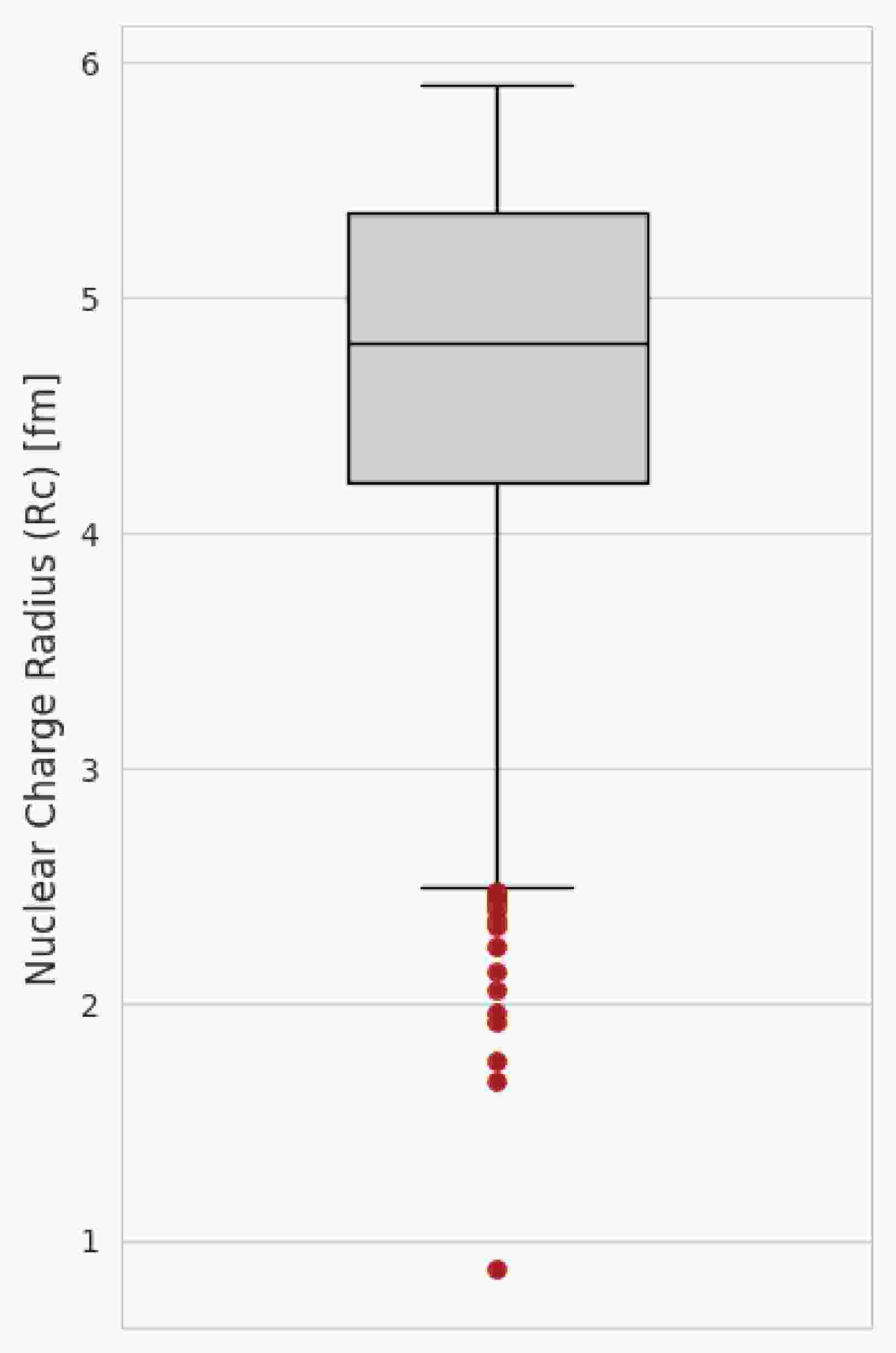
Based on this technique, 17 out of 1040 nuclei were falling outside the lower fence. Figure 1 shows the resulting box plot with outliers highlighted in red, and Table 1 lists the corresponding nuclides.

Figure 1.  (color online) Box-plot of $ R_c $ using 1.5×IQR rule

Sr.#	A	N	Z	$ R_c $ (fm)
1	1	0	1	0.8783
2	2	1	1	2.1421
3	3	2	1	1.7591
4	3	1	2	1.9661
5	4	2	2	1.6755
6	6	4	2	2.0660
7	8	6	2	1.9239
8	7	4	3	2.4440
9	8	5	3	2.3390
10	9	6	3	2.2450
11	11	8	3	2.4820
12	10	6	4	2.3612
13	11	7	4	2.4669
14	10	5	5	2.4277
15	11	6	5	2.4060
16	12	6	6	2.4702
17	13	7	6	2.4614

Table 1.  Nuclides flagged as outliers by Tukey’s 1.5 × IQR rule on $ R_c $.

The theoretical ground state properties were only available for the nuclides ranging from oxygen (Z = 8) to darmstadtium (Z = 110), and 26 nuclides had missing values of theoretical ground state properties. We simply excluded these isotopes from our study; therefore, our study was restricted to the range between oxygen (Z = 8) and curium (Z = 96). The reasons behind exclusion are that 17 nuclei of them were flagged as outliers, and the remaining 9 isotopes were also removed to keep our data complete (without missing entries). Finally, we ended up with the consolidated data table of charge radii of 1014 isotopes with predictors N, Z, theoretical BE, S_2n (two-neutron separation energy), and S_n (one-neutron separation energy). Including mass number (A) would add perfect multicollinearity with neutron number and proton number (since $ A = N + Z $), and would provide no independent information, and our preliminary tests showed no improvement in predictive performance. Its exclusion thus can enhance the model stability and preserve the clarity for SHAP-based feature importance analysis. However, as detailed in Section 3.2, S_n and S_2n were subsequently removed from the feature set for the final model.

In the feature selection phase, a very lightweight CatBoost model was trained with iterations = 500, learning_rate = 0.1 for quick insight into the candidate features and to select the most promising ones. A random seed of 42 was maintained to ensure the reproducibility of the feature selection process. Rather than training on a single random test/train split, we k-fold cross-validated (described in Section 3.4) on shuffled 10-folds but with a fixed random seed of 42. In this exploratory lightweight model's feature score (as shown in Fig. 2), neutron number, BE, and proton number were the most influential features, with mean importance of 36.8%, 28.1%, and 26.7,%. Based on these insights, we dropped less important features, i.e., S_n and S_2n, corresponding to the theoretical S_n and S_2n, which demonstrated very low mean importances (4.6% and 3.8%, respectively) and were therefore dropped from the final model. With only three features mentioned above, we were getting very promising predictive performance therefore we reduced our feature set to three features only and to demonstrate that CatBoost works well even with limited features.

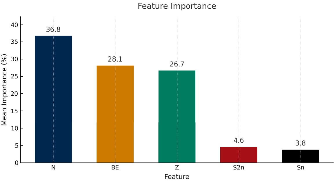
Figure 2.  (color online) Preliminary feature-importance bar plot of selected candidates

The model was then tuned for the best possible predictive performance by searching for optimal hyperparameters. Hyperparameters are selected via Optuna’s Tree-Structured Parzen Estimator (TPE) sampler. The search was performed with 10-fold cross-validation by targeting the minimum average RMSE across all folds. In total, 200 Optuna trials were executed, and each trial's metadata was stored in a relational database file, which we queried later to analyze search history using the Optuna “best-so-far” plot (Fig. 4), and hyperparameter interactions were studied using a parallel-coordinate plot (Fig. 5). The full search space is summarized in Table 2.

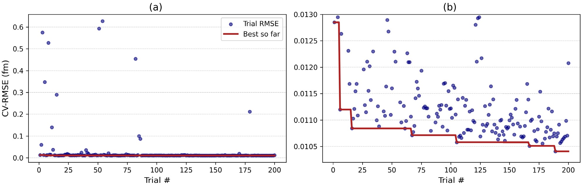
Figure 4.  (color online) Optuna CV-RMSE progress over 200 trials. (a) Full-range CV-RMSE history for all trials. (b) Zoomed-in view (outliers clipped).

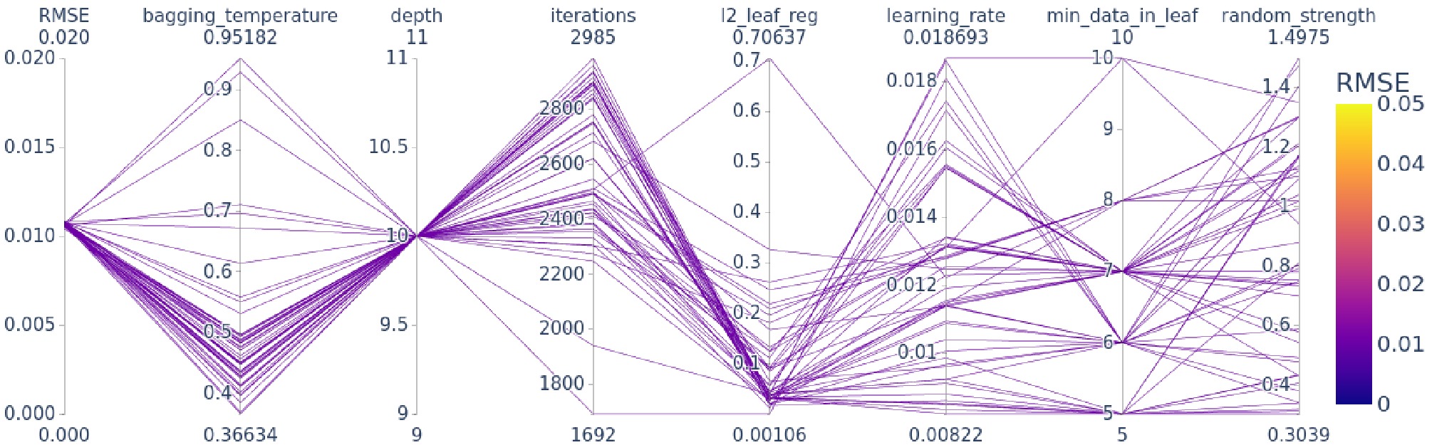
Figure 5.  (color online) Parallel-coordinates plot of the top 50 Optuna trials, showing the sampled hyperparameter values and their corresponding 10-fold CV-RMSE (color-coded).

Hyperparameter	Type	Search Range	Scale
iterations	integer	1000–3000	linear
learning_rate	float	$ 10^{-4} $–$ 10^{-1} $	log
depth	integer	6–12	linear
l2_leaf_reg	float	$ 10^{-3} $–10	log
random_strength	float	0.0–2.0	linear
bagging_temperature	float	0.0–1.0	linear
min_data_in_leaf	integer	5–20	linear

Table 2.  Search space for CatBoost hyperparameters.

To assess the predictive performance and reliability of our model, we rigorously evaluated our model in a systematic protocol.

Error Metrics: Three standard regression metrics for performance evaluation have been used on both 10-fold cross-validation and unseen hold-out sets:

where N denotes the number of samples (isotopes in our case), $ y_i $ the true (experimental) charge radius, and $ \hat y_i $ the predicted charge radius by Catboost.

● Mean Absolute Error (MAE) calculates simple average absolute deviation. Since it weights all equally, this makes it robust and relatively less sensitive to large errors.

● Root Mean Squared Error (RMSE) is the most commonly used metric in regression studies. It squares errors, computing averages, which penalizes larger errors more heavily, thus making it robust to highlight significant prediction failures.

● Mean Absolute Percentage Error (MAPE) describes errors as percentages of actual values, allowing scale-independent comparison between different measurement ranges. Moreover, the percentage error is always more intuitive than all other metrics.

Cross-Validation: The whole training dataset (80% of the total, i.e., 811 nuclides) was segregated into 10 equal samples via random sampling, and then training and testing were performed on these ten samples. Each time, nine samples were used to train, and the remaining sample was used as a validation set. This 10-fold CV was used both for hyperparameter tuning and to report error metrics (with standard deviation) over all folds (see Table 3 in section (4) for fold-wise RMSE, MAE, and MAPE, plus mean ± SD and hold-out results).

Hold-Out Test: To ensure the robustness and reliability, the final hyperparameter-tuned model was then tested on a fully unseen holdout test set of 203 nuclei. Final performance is reported on the 203-nuclide test set. This procedure diagnoses overfitting and allows robust assessment of the model's accuracy for real-world predictions.

Comparative Benchmarking: Results are compared against nine recently reported machine-learning methods (RF, QRF, Cubist, XGBoost, GPPK, MARS, SVR, ANN, and CNN) [31, 54] and the BRUSLIB BSkG3 [55] theoretical data library for ground state properties based on Hartree-Fock-Bogoliubov (HFB) with Skyrme Energy-Density Functional. All the models are compared while treating experimental measurements as the gold standard.

Interpretability: The performance of CatBoost is interpreted using residual analysis, parallel-coordinate plot, and SHAP summary analysis.

● Residual Analysis: Discrepancy plots and predicted-vs-true scatter (Fig. 3) were used for residual analysis and to highlight any systematic biases.

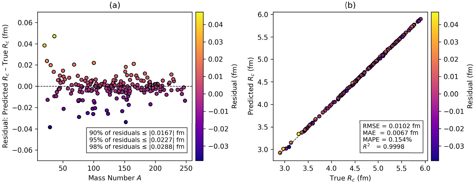
Figure 3.  (color online) (a) Discrepancy Plot of Residuals (Predicted $ R_c $ - True $ R_c $) vs mass number A. (b) Predicted versus true $ R_c $.

● Hyperparameter Insights: The Optuna “best-so-far” plot (Fig. 4) was used to track convergence history, while parallel-coordinate plots (Fig. 5) revealed key insights into hyperparameter interactions.

● Feature Contributions: SHAP values were computed on the training data, and a beeswarm SHAP summary plot was used to rank feature importances and to interpret our model.

This rigorous, systematic and comprehensive evaluation protocol makes our conclusion about the model performance and claim of superiority over other models physically meaningful and statistically sound.

This section presents the analysis of our CatBoost model's accuracy and performance on charge radii predictions. First, we present a summary of 10-fold cross-validation results on the training set by using performance metrics RMSE, MAE, and MAPE to examine the overall stability across 10-fold isotopic splits. Then we analyze the model's performance on hold-out unseen tests and quantitatively compare our model's predictive abilities with recently reported machine learning algorithms. Then, we analyze the outcome of hyperparameter tuning, followed by a feature interactions study and SHAP analysis. Finally, we use our trained model to predict krypton and strontium isotopic chains to compare our CatBoost predictions with theoretical models (BSkG3 and PC-X) and previously reported machine learning algorithms.

Table 4 provides a quick summary of error metrics of the CatBoost model, while Table 3 presents the detailed fold-wise error metrics. The holdout test RMSE was 0.0102 fm, which is quite low, demonstrating a very good predictive performance on unseen real-world predictions. The mean RMSE of 10 folds was 0.0106 fm with a standard deviation of 0.0030 fm. The fold-wise RMSE ranged between 0.0070 fm and 0.0182 fm, where the upper value is still lower than many models' average of 10-fold error (Table 5). The 10-fold average of MAE and MAPE was 0.0067 fm with a standard deviation of 0.0011 fm and 0.157% with a standard deviation of 0.033% respectively, demostrating remarkable predictive accuracy. In K-fold CV, we found that eight out of 10 folds demonstrated RMSE below 0.012 fm. This consistent low error suggests that the model was stable and not sensitive to variations in training-validation splitting. In summary, consistently low error is evidence that our model was able to capture the underlying relations between the charge radius and our features (N, Z, BE).

In Fig. 3, we present a two-way perspective on the model's generalization performance. In panel (a), residuals ($ \text{Predicted } R_c - \text{Actual } R_c $) are plotted against the atomic mass number A, and color encoding indicates the magnitude of residuals. This plot reveals that most of the points are tightly concentrated at the central zero error line, with very few outliers. The inset quantifying the residual distribution is added, which shows that 90%, 95%, and 98% of the absolute errors are below 0.0167 fm, 0.0227 fm, and 0.0288 fm, respectively. This proves that the model's errors are consistently low, and very few predictions have errors beyond 0.03 fm. Importantly, no systematic bias over the whole range of mass numbers is observed. A few outliers can be seen with relatively higher residuals, suggesting the model's limitation in the scarce light-nuclei region of the nuclear chart. Panel (b) illustrates the correlation between predicted and true charge radii, which is an excellent agreement along the ideal $ y=x $ line. The inset in the panel (b) shows the performance metrics showing RMSE = 0.0102 fm, MAE = 0.0067 fm, MAPE = 0.154%, and $ R^2 $ = 0.9998, which means that our model can explain approximately 99.98% of the variance in the nuclear charge radius.

In Table 5, we side-by-side compare our model's 10-fold cross-validation and hold-out test errors with a range of alternative data-driven algorithms [31, 54]. Notably, CatBoost outperforms all other algorithms by delivering the smallest 10-fold CV with RMSE 0.0106 fm and MAE 0.0067 fm, as well as the lowest test RMSE 0.0102 fm and MAE 0.0067 fm. The closest competitor of CatBoost is Cubist, which achieves a CV-RMSE of 0.0120 fm with the same test RMSE. XGBoost, Random Forest, and Quantile Random Forest rank third, fourth, and fifth in the competition, respectively, whose CV errors exceed CatBoost’s by roughly 15-30%. Gaussian Process polynomial Kernel (GPPK), Multivariate Adaptive Regression Splines (MARS), Support Vector Regression (SVR), and Artificial Neural Networks (ANN) exhibit relatively larger errors (CV-RMSE up to 0.04286 fm, test RMSE up to 0.0564 fm), while the CNN exhibits a test RMSE of 0.0156 fm. In other words, GPPK, MARS, SVR, and ANN are roughly three to four times less accurate than CatBoost (see Table 5). These results establish the fact that CatBoost excels in nuclear charge-radii modeling, combining the lowest errors in both cross-validation and hold-out testing. Its consistent superior performance, especially against modern algorithms like Cubist, XGBoost, etc., demonstrates CatBoost’s robust generalization ability. This highlights the potential of CatBoost in nuclear science, particularly in ground state properties and nuclear structure, leading to efficient and more accurate modeling of nuclear structure and even nucleosynthesis.

In Fig. 4, we present a full-scale optimization history (panel a) and a zoomed-in view of the best-so-far trajectory (panel b) of Optuna-driven 10-fold CV hyperparameter search over 200 trials. If we discuss the first 50 trials, in panel (a), trial 0 begins at 0.012849 fm, then for exploration it spikes at trial 1 (0.060102 fm) and trial 2 (0.574825 fm), then settles back to 0.012948 fm at trial 3. We see a prominent improvement at trial 5, where CV-RMSE falls to 0.011198 fm. In subsequent trials (6-49), CV-RMSE oscillates mostly between 0.010880 fm (trial 38) and 0.015588 fm (trial 24), with occasional higher values at trials 10 (0.139897 fm), 14 (0.289320 fm), 35 (0.024157 fm), and 39 (0.035871 fm) as the sampler initially explores various hyperparameter regions.

Panel (b) downscaled on the best-so-far CV-RMSE trajectory, also present in panel (a), but with extreme outliers clipped off to show the evolution of optimization effectively. The best-so-far curve descends as the trials proceed until trial 188 achieves the minimum CV-RMSE of approximately 0.0104 fm. This trial remains the best through trial 200. This evolution of rapid early descent followed by continuous fine-tuning confirms that our 200-trial search was both efficient and sufficient to search the optimal CatBoost hyperparameters for the prediction of nuclear charge radii. We note that additional trials might slightly reduce CV-RMSE, but since we achieved the desired performance and it stabilized by trial 200, therefore we limited our search to 200 trials to balance accuracy and computational cost. To study the interactions among the hyperparameters, we filtered out the top 50 trials (with the lowest CV-RMSE) and visualized them using the parallel-coordinates plot among the CV-RMSE and all the hyperparameters. Fig. 5 shows a parallel-coordinates plot of the 50 Optuna trials with the lowest 10-fold CV-RMSE. Each line tracks one trial’s hyperparameter settings, i.e., number of iterations, learning rate, tree depth, $ l_2 $-leaf regularization, bagging temperature, minimum data in leaf, and random strength, and is color-encoded by its corresponding CV-RMSE. Interestingly, all the best configurations use a single depth of 10 and learning rates spread between 0.008 and 0.018, iteration counts lie toward the upper end of the search range, and mostly spread between 2300 and 2985. $ l_2 $- Leaf regularization mostly remains below 0.15, bagging temperature falls in a moderate range, i.e. between 0.4 and 0.55, and minimum data in leaf is clustered on 5, 6, 7, and 8. The random strength is almost equally spread between 0.8 and 1.4. In Table 6, we report the best found hyperparameter values from trial 188 in Optuna. Using these parameters on our processed data, one can reproduce the exact CatBoost model with exact predictions and evaluation metrics, highlighting full reproducibility of this work.

In Fig. 6, we present a SHAP (Shapley Additive exPlanations) beeswarm plot that quantitatively analyzes how each input feature impacts the predictions of nuclear charge radii by the CatBoost model. The features are ordered from top to bottom based on the mean SHAP value. This highlights that PC-X BE is the most influential feature, followed by Z and N. Each point in the plot corresponds to an individual nuclide from the training set, horizontally positioned based on its SHAP value, which reflects its specific impact on the predicted radius, and color-encoded to show the actual value or magnitude of the corresponding feature value from blue to red (low to high). We note that all three features demonstrate both positive and negative SHAP contributions: nuclei with higher BEs, proton numbers, or neutron numbers systematically exhibit positive SHAP values, corresponding to larger predicted radii. This outcome is quite obvious and aligned with established nuclear theory, where greater proton and neutron numbers naturally lead to larger nuclear sizes due to increased nucleon occupancy in nuclear shells. Likewise, total BE grows with mass number A, and because charge radius scales as $ R \approx A^{1/3}, $ nuclei with higher BE usually produce positive SHAP contributions, so in general (for local chain-level, see Section 4.3.1), charge radius increases with an increase in BE. Conversely, lower BE corresponds to a negative SHAP value, reflecting smaller charge radii.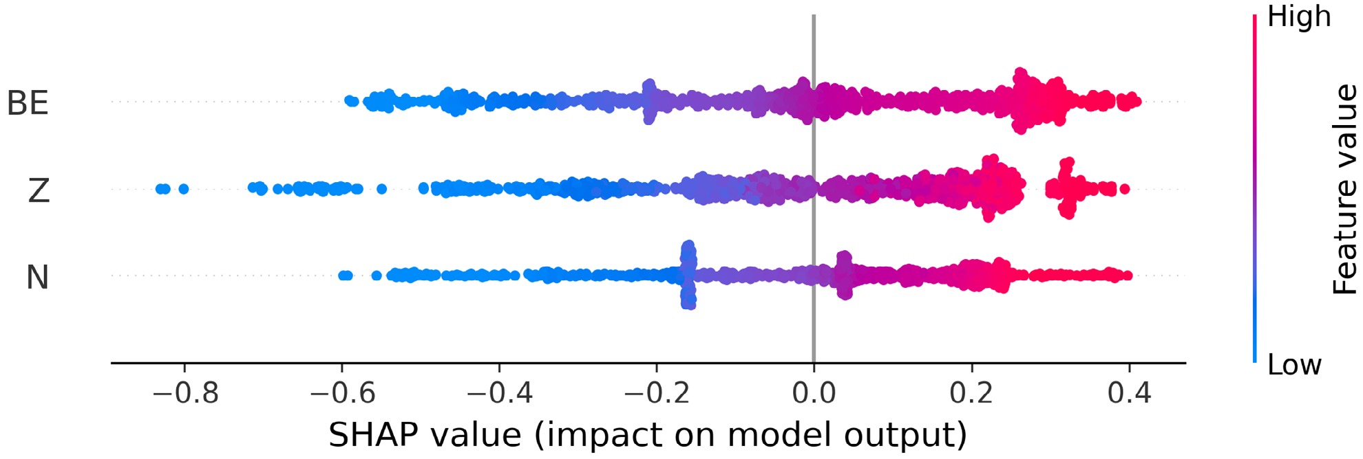

Figure 6.  (color online) Beeswarm plot of SHAP values for the CatBoost charge-radius model.

Quantitatively (see Table 7), BE achieves the highest mean absolute SHAP (0.223), followed by Z (0.213) and N (0.176), demonstrating that it drives model output more strongly on average. Z exhibits the largest SHAP range (-0.83 to +0.39), showing that extreme atomic numbers can both strongly increase and decrease predicted radii. The near-zero mean SHAP values ($ Z\approx3\times10^{-5} $, $ N\approx1.4\times10^{-3} $, BE$ \approx-1.5\times10^{-3} $) indicate that positive and negative effects balance each other across the training set. This implies that the model is well balanced and does not overly overestimate or underestimate the predictions. In conclusion, this SHAP analysis confirms that BE is the most influential feature overall, consistent with its fundamental role in nuclear structure, followed by neutron number and proton number. This highlights that the inclusion of theoretical BE in the dataset as a feature has helped the model to generalize well over the data and improve prediction accuracy.

Feature	Mean SHAP	Mean |SHAP|	Span (max–min)	Range (min to max)
Binding energy (BE)	$ -0.00145 $	0.2234	0.9990	$ -0.5898 $ to $ +0.4092 $
Proton number (Z)	$ 0.00003 $	0.2132	1.2248	$ -0.8305 $ to $ +0.3942 $
Neutron number (N)	$ 0.00142 $	0.1759	0.9955	$ -0.5977 $ to $ +0.3978 $

Table 7.  SHAP value summary: mean SHAP, mean absolute SHAP, span, and min-max range, ordered by descending mean absolute impact.

We also explore the localized SHAP for Sr (Z = 38) and Kr (Z = 36) chains, computed using an interventional TreeExplainer on a global background sampled from the whole training set. This common baseline stabilizes the sign and scale of attributions and we interpret results within each chain.

The chain-level beeswarms (Fig. 7) shows that at the chain level neutron number N is the dominant feature (largest horizontal spread), Z is negligible inside each chain (constant value), and BE is a secondary, often negative contributor in this local neutron window. The dependence plot of $ {\rm{SHAP}}(N) $ on N (Fig. 8) shows a sharp minimum at $ N \approx 50 $. For $ N<50 $ adding more neutrons yields negative contributions (model predicts charge radius below the global expectation), whereas for $ N>50 $ the contributions recover toward zero, indicating a trend reversal across the shell closure. When $ BE $ is included as a feature, color-coding shows that although $ BE $ rises with N, the most negative $ {\rm{SHAP}}(N) $ appears near $ N \approx 50 $, demonstrating that at magic number, the local shell effects can override the global trends.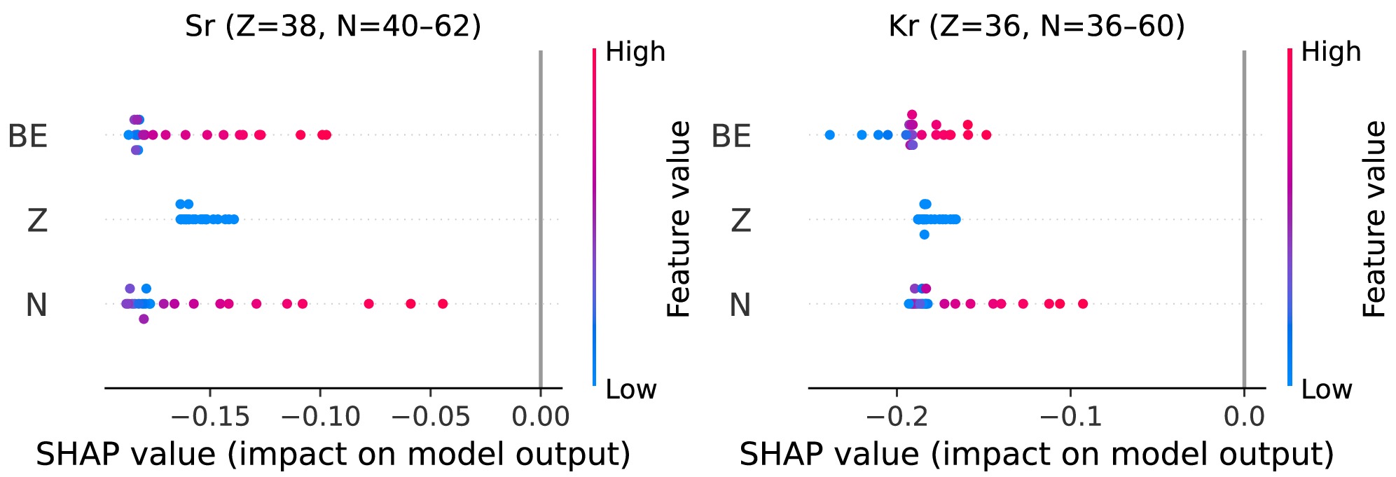

Figure 7.  (color online) Localized SHAP (beeswarm) for Sr (Z=38) and Kr (Z=36) with a single global background. Within each chain, N dominates; Z is near zero (constant locally).

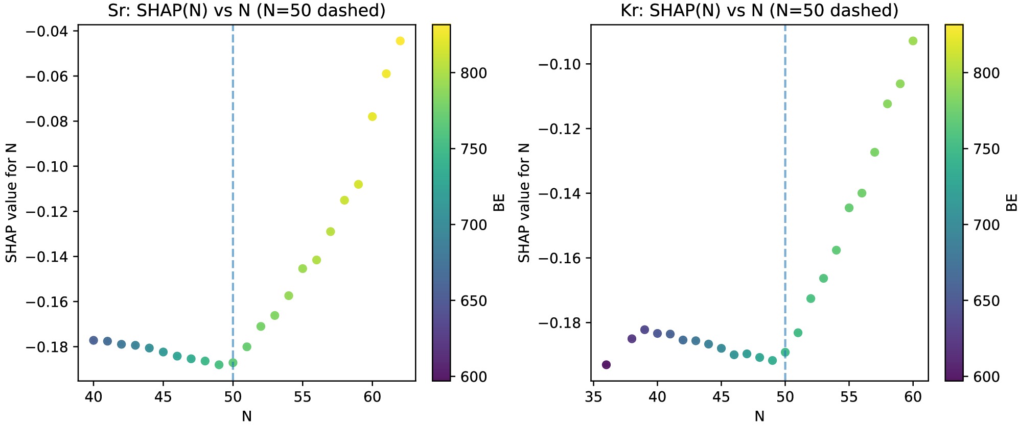
Figure 8.  (color online) $ {\rm{SHAP}}(N) $ versus N with $ N=50 $ marked. Both chains show a minimum near $ N \approx 50 $ (negative for $ N<50 $, recovery for $ N>50 $).

Variations in the charge radii within isotopic chains encode the deformation, shell effects, and pairing properties, making isotopic chain patterns a cornerstone of nuclear structure investigations. Reproducing these isotopic chain trends with high accuracy can be used as a litmus test to assess any predictive model, ranging from a basic empirical model to a complex mean field model and even data-driven algorithms. To make our claim of our model's superiority over others more strong, we focus on krypton (^72-96Kr) and strontium (^78-100Sr), which exhibit the shell-closure “kink” at N = 50, the odd-even staggering due to pairing effects. This comparison allows us to critically assess how well our model captures the underlying physics behind nuclear charge-radius variations. Moreover, both these isotopic chains lie on or near potential astrophysical r-process pathways. Therefore, an accurate description of these chains can improve the nucleosynthesis models and our understanding of heavy element formation in the universe.

In Fig. 9(a), we present a comparison of CatBoost against Cubist, Random Forest (RF), and Quantile Regression Forest (QRF), using experimental data as a standard benchmark. CatBoost’s prediction data points not only follow the overall trend but also coincide with the experimental points (except A = 75) across A = 72-96, accurately reproducing the N = 50 shell-closure kink at A = 86. RF and QRF also follow the overall trend but consistently overestimate the charge-radius values, with several larger deviations. Cubist shows a prominent error at A = 78, and after the shell-closure kink point, it becomes excessively steep and overshoots the charge-radius values. On the other hand, CatBoost gives predictions of both even and odd masses, and its odd-A predictions faithfully align with the experimental odd-A charge radii values.

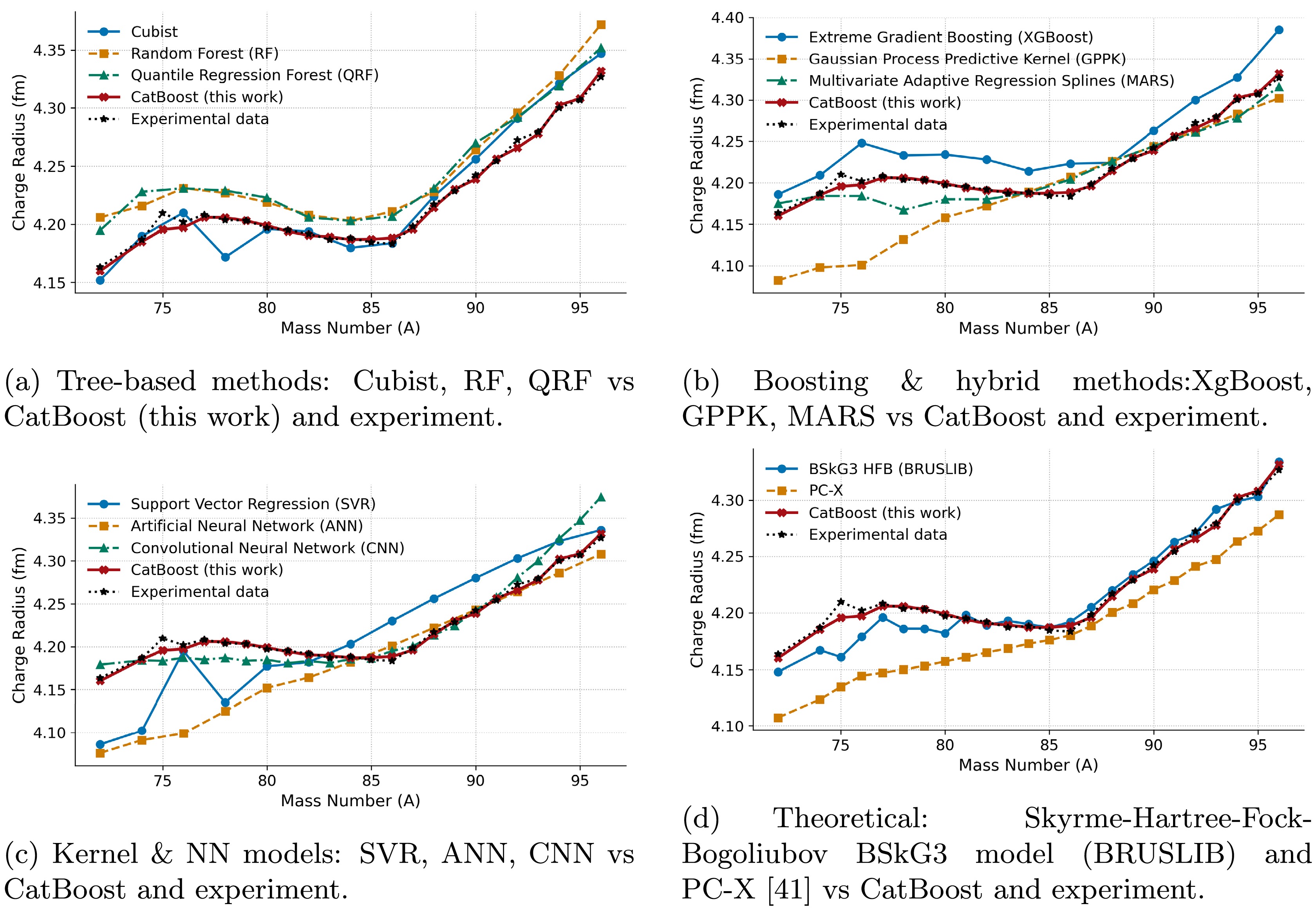
Figure 9.  (color online) Charge-radius predictions for the $ ^{72\text{-}96}{\rm{Kr}} $ chain. CNN and experimental data cover both even and odd-A (note $ A= 73 $ is unavailable experimentally). Therefore, A = 73 data point was dropped. Other models (RF, QRF, Cubist,XgBoost, GPPK, MARS, SVR, ANN and PC-X) report only even-A values, hence gaps visible at odd-A.

In Fig. 9(b), we compare CatBoost against Extreme Gradient Boosting (XGBoost), the Gaussian Process Predictive Kernel (GPPK), and Multivariate Adaptive Regression Splines (MARS). Similar to RF and QRF, XGBoost also consistently over-predicts the charge radii values and shows a steep slope after A = 50, producing a larger deviation from the experimental values. GPPK under-predicts with quite large errors below A = 80 and then oversmoothes the data points, producing a too flat curve, which shows its inability to reproduce actual chain trends and capture odd-even staggering and kinks at shell closure. MARS, while closer to the experimental slope, underestimates several points between A = 74 to 82. But overall, it follows the trend and captures the kink at shell closure relatively better than tree-based models. But despite this, CatBoost predictions are still superior to those of MARS, as demonstrated by precisely overlapping experimental data points and capturing the chain trend.

In Fig. 9(c), Support Vector Regression (SVR) underestimates the radii predictions at the low-A end, and at A = 82 it shows an almost constant slope, deviating significantly from experimental values, showing its inability to capture both trend and shell-closure kink. The Artificial Neural Network (ANN) likewise underpredicts the overall trend but accurately predicts in the mid-A range, as shown in the figure. The Convolutional Neural Network (CNN) gives both even and odd A predictions and accurately captures N = 50 kinks and slightly overpredicts radii in the neutron-rich end.

In Fig. 9(d), we see a comparison of our model with the theoretical BSkG3 model (Skyrme-Hartree-Fock-Bogoliubov). We extracted this data from the Brussels Nuclear Library for Astrophysical Applications (BRUSLIB). Although it captures the chain trend effectively and precisely predicts the odd-even oscillations as well as the kink at N = 50. But it underestimates the charge radii values in the lighter half of the chain until A = 82, which highlights its limited performance for the neutron-deficient range.

In Fig. 10, we present the same comparison for the strontium chain. In the Strontium chain ($ A = 78-100 $), classical tree models (Cubist, RF, QRF) show a relatively good fit with shell-closure kink but also come with localized deviations at multiple points larger than Catboost's predictions. XGBoost follows the overall trend, captures the kink at shell closure, but yet overestimates beyond A = 96, therefore having lesser predictive performance than CatBoost. GPPK and MARS underestimate at both the light- and heavy-mass ends and produce overly smooth, too-flat profiles that diverge from experimental values. SVR also demonstrates a too-flat line, misses the N = 50 kink and overall trend pattern, while ANN underestimates both heavy-mass and light-mass end radii and only fits relatively well in the mid-range (A = 86 to 97). Among all approaches (except CatBoost), CNN exhibits the closest fit but still deviates from A=95 to 97. The BSkG3 model reproduces the kink and accurate charge radii between A=85 and 95 but underestimates radii below A = 80.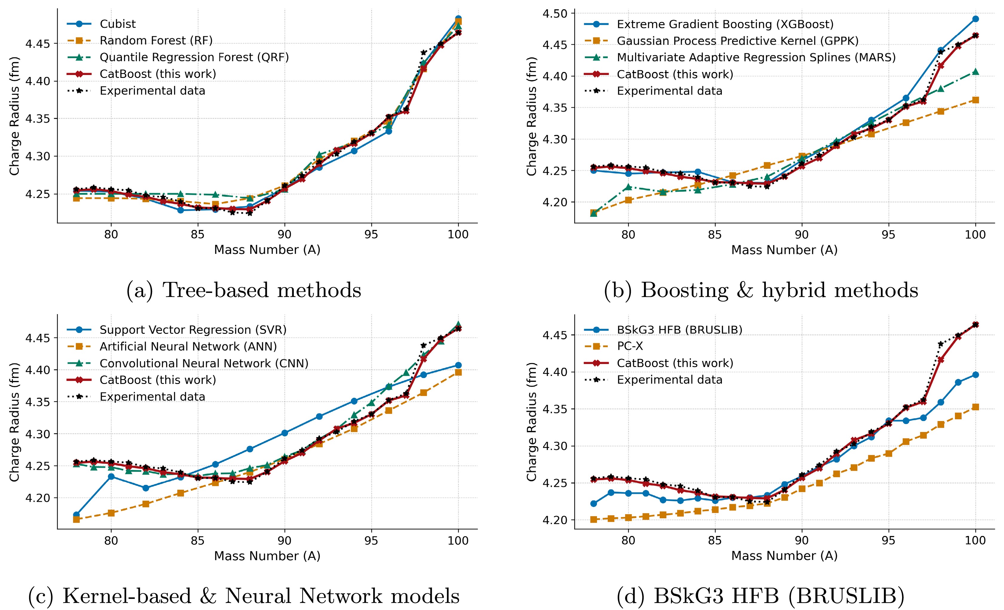

Figure 10.  (color online) Same as Fig. 9, but for the ^78-100Sr chain.

The CatBoost model consistently outperforms all the models in the prediction of both krypton and strontium chains, simultaneously capturing the shell-closure kink and the subtle odd-even oscillations while accurately following the overall trend. Although individual models (tree models, boosting, ANN, CNN, and BSkG3) [31, 54, 55] each excel in one or two aspects, none are best in all at once. CatBoost excels at all these qualities simultaneously, which proves its predictive superiority against these models and suggests that it can be a highly promising approach for ground state properties predictions, including charge radii, error quantification, and refinement of nuclear models.

In the present analysis, we report the first utilization of the CatBoost model for more accurate ground-state nuclear charge radii computations across 1014 nuclides. In order to create a high-quality dataset that is larger than prior research, we combine two extensive experimental compilations (Angeli & Marinova; Li et al.). We also incorporate physics-informed features from PC-X computations. An Optuna driven hyperparameter search was conducted to minimize the average 10-fold cross validation RMSE to 0.0106 fm, and (MAE = 0.0067 fm, MAPE = 0.154%) yielded a hold-out test RMSE of 0.0102 fm (MAE = 0.0067 fm, MAPE = 0.154%). SHAP analysis indicated that BE had an advantageous influence on the model's performance and appeared as the leading predictor, which is consistent with nuclear theory. The residual analysis revealed no significant consistent bias throughout nearly entire atomic mass range. When compared to nine established machine learning methods and the BRUSLIB library (BSkG3), CatBoost displayed higher global predictive power and stability. Notably, our model accurately modeled isotopic properties including the N = 50 shell-closure kink and odd even staggering in Kr and Sr chains, demonstrating its excellent generalizability. These findings establish CatBoost as a potent, interpretable tool for nuclear radius prediction, paving the path for future enhancements such as enlarged feature sets, uncertainty quantification, and hybrid modeling using ab initio techniques.