Universal momentum distributions for the spin-singlet NN channels

The problem of short-range correlations (SRC) is very relevant nowadays due to recent theoretical and experimental achievements [1−8]. The new experiments allow us to count correlated nucleon pairs with high relative momentum and small center of mass momentum. The theoretical description of the corresponding cross-sections in quasi-elastic kinematics is reduced, in many cases, to treatment of the momentum distributions of nucleons in nuclei. This gives rise to the contact formalisms [9, 10], which appear to be convenient for practical calculations [5].

In this paper, we discuss one of the key aspects of the SRC problem. The two-nucleon momentum distribution $ \rho^A_{ { {NN}}} $ in the nucleus A depends on the relative momentum of nucleons k, the momentum of their center of mass Q, and the angle θ between the corresponding vectors. These distributions have similar properties for different nuclei [11] and satisfy the factorization property at high relative momenta k and low Q [9, 12]:

where $ C^A_{ { {NN}}} $ is a constant depending on the nucleus A (the so-called nuclear contact), $ \rho^{A, { {NN}}}_{\rm{cm}}(Q) $ is a distribution of center-of-mass momentum for a pair of nucleons in the nucleus, while $ \rho_{ { {NN}}}(k) $ represents a universal two-nucleon momentum distribution (UMD) that does not depend on A [9]. The high-momentum part of this distribution depends on the chosen model of $ NN $ interaction. In the case of spin-triplet $ np $ pairs, this universal distribution coincides with the distribution of nucleons in the deuteron: $ \rho_{np}(k) = \rho_d(k) $. Because $ \rho_d(k) $ is normalized to 1, one can explicitly calculate a weight of the high-momentum part of the distribution $ a_2^d $ [13], which determines the magnitude of SRC.

At the same time, for spin-singlet $ ^1S_0 $ $ NN $ channels (i.e., $ np $, $ pp $, and $ nn $), bound states are absent and there is a problem of determining the corresponding universal distributions [9], as well as estimating the magnitude of high-momentum components for such states for two-nucleon system. In [12], the corresponding momentum distributions at $ Q = 0 $ in $ ^4 {\rm{He}}$ were considered as universal distributions for $ pp $ (or $ nn $) pairs, and factorization (1) was used to calculate spectral functions for heavier nuclei up to $ ^{40} $Ca. Another approach to determining the UMD for spin-singlet pairs was proposed within the Generalized Contact Formalism (GCF) [5, 10] by using the two-body $ NN $ scattering wave functions at zero energy, which are normalized by their high-momentum tails, i.e., the integral from some $ p_0 $ (the boundary of the high-momentum region) to infinity. However, the problem of quantitatively evaluating the high-momentum components for spin-singlet channels, which would allow comparison of different $ NN $ interactions in this regard, still remains open.

In the present paper, we propose a universal distribution for singlet $ NN $ channels that does not depend on the boundary of the high-momentum region $ p_0 $ and is determined directly by the momentum distribution for the virtual state. It should be noted that such a distribution for a particular case of a separable $ NN $ interaction was used as a two-body $ pp $-distribution in Ref. [14]. In a general case, to obtain the momentum distribution for virtual state, one can use the low-energy scattering wave functions.

For this purpose, we use the approach of Fäldt and Wilkin [15, 16], which established a relation between the scattering and bound state wave functions and was applied to inelastic $ NN $ scattering calculations [17]. This approach gives an explicit factor (the Fäldt-Wilkin factor) that allows the bound- and virtual-state momentum distributions to be approximately reproduced in the high-momentum region by using the low-energy scattering wave functions. As a result of the developed technique, we introduce high-momentum constants for different $ NN $ interactions in the spin-singlet channel and compare quantitatively high-momentum parts of momentum distributions for different models of $ NN $ interactions. Our recently suggested treatment [18] for high-momentum components of the scattering wave functions is helpful for this.

As a numerical illustration, we calculate the nuclear contacts for $ pp $ momentum distributions in $ ^3 {\rm{He}}$ with respect to the introduced two-nucleon momentum distributions for four realistic but essentially different models of $ NN $ and $ 3N $ interaction and show that these contacts have nearly the same values. Thus, the suggested formalism can be considered as an extension of the formalism presented in Ref. [9] for $ np $ triplet momentum distributions.

The paper is organized as follows. In Sec. II, we derive a relation between the scattering and bound- or virtual-state wave functions and define an explicit factor, i.e., the Fäldt–Wilkin factor. In Sec. III, the found relations are tested for the separable interaction when the virtual-state momentum distribution is found analytically and for the realistic $ NN $ interaction as well. In Sec. IV, the UMDs for the spin-singlet $ NN $ channels are introduced based on the developed formalism, and the values of the high-momentum constants $ a_2^v $ are presented for four different models of $ NN $ interaction. In Sec. V, the nuclear contacts for the $ ^3 {\rm{He}}$ nucleus are calculated based on the two-nucleon UMDs. A summary is given in Sec. VI. For the reader's convenience, a small Appendix A gives the explicit relations between different universal momentum distributions.

Let's start with the definitions which we will use below.

For the spin-triplet bound state, the two-nucleon momentum distribution is naturally introduced by using the deuteron wave function with the S-wave and D-wave components $ u(k) $ and $ w(k) $, respectively:

The S-matrix $ S(p) $ for the spin-triplet $ np $-scattering (here, $ p = \sqrt{2\mu E/\hbar^2} $ is the on-shell momentum) has a pole in a complex p-plane at $ p = {\rm i} \varkappa_d $, where $ \varkappa_d\equiv \sqrt{-2\mu E_d/\hbar^2}>0 $ is the wave number corresponding to the bound-state energy $ E_d $, and μ is the reduced mass of two nucleons.

The corresponding residues of the S-matrix elements at this pole determine the asymptotic normalization coefficients (ANCs) $ N_S $ and $ N_D $ (see Sec. II.D), which set amplitudes of components of the deuteron wave function in configuration space at $ r\to \infty $:

provided that the deuteron wave function is normalized to unity: $ \int_0^\infty [u^2(r)+w^2(r)]{\rm d}r = 1 $.

There are no bound $ NN $ states in the spin-singlet channel $ ^1S_0 $. However, in this channel, there is a virtual state $ u_v(r) $ with $ E_v<0 $ (for the $ np $ system $ E_v \approx -67 $ keV). The pole of the S-matrix corresponding to the virtual state lies on the unphysical energy sheet and on the negative imaginary semi-axis in the complex p-plane at $ p = {\rm i} \varkappa_v $:

The function $ u_v(r) $ grows exponentially at the asymptotics:

in contrast to the bound-state case. However, the constant $ N_v $ in Eq. (5) is the ANC for a virtual state, which is related to the residue of the S-matrix $ S(p) $ for the singlet state at the pole $ p = {\rm i} \varkappa_v $.

It should be noted that although the virtual state function in the coordinate representation $ u_v(r) $ with the asymptotics (5) cannot be normalized, the virtual state wave function in the momentum representation $ u_v(k) $ is square integrable [19] (also see the example with a separable potential in Sec. III). One can also define a special Fourier transform procedure that relates the coordinate and momentum representations for the virtual-state wave function [20].

Therefore, one can consider the momentum distribution for the virtual state in a similar manner as for the bound-state (2) as follows:

This distribution has the same dimension as for the bound-state, however, it is not normalized to unity. It would be convenient to define the UMD for the spin-singlet $ NN $ channels based on these distributions for virtual states. However, a practical calculation of such a momentum distribution could be complicated for realistic $ NN $ interactions. Thus, we will show how to reconstruct it in the high-momentum region just from the low-energy scattering wave functions for the same interaction.

Finally, we introduce the scattering wave functions here. Below, we consider the radial parts of the scattering wave functions $ \psi_p^s $ and $ \psi_{p,l = 0,2}^t $ for two main $ NN $ configurations $ ^1S_0 $ and $ ^3S_1 $-$ ^3D_1 $ both in coordinate and momentum representations. In the momentum space, these functions are normalized as follows:

where p is the on-shell momentum.

In the configuration space, we consider functions that satisfy the asymptotic condition of a standing wave. For a singlet channel, this means

where $ \phi(p) $ is the partial phase shift.

In Ref. [15], the authors found an explicit relation between bound-state and scattering wave functions for the same Hamiltonian in case of the S-wave interactions (without tensor coupling) by using an analytical continuation of the scattering wave function to the bound-state pole of the S-matrix. For our purposes, we also require a similar relation for the virtual state. Thus, let us briefly reproduce the derivation from Ref. [15] with some minor changes in notations.

Near the pole $ p = {\rm i} \varkappa $ corresponding to the bound or virtual state, the S-matrix can be presented in the form

For a bound state, the constant N in Eq. (9) is a corresponding ANC (see [21, 22] and references therein). Near the pole, the relation (9) can also be written in the form

where $ \varkappa>0 $ for a bound state and $ \varkappa<0 $ for a virtual state.

The asymptotics of the wave function of both bound and virtual states in the configuration space can be written in a unified way:

At the same time, the scattering wave function has the following asymptotics:

where in agreement with (8),

Near the pole $ p = {\rm i} \varkappa $, $ \phi\to -{\rm i}\infty $, $ C^{(-)}(p)\to 0 $; hence,

Comparing Eqs. (10) and (13), one can find an explicit relation between $ C^{(+)} $ near the pole and ANC N:

The quantity

is referred to as the Fäldt-Wilkin's Factor (FWF).

Combining Eqs. (11), (14), and (15), we obtain the following relationship between the wave functions of the discrete and continuous spectra

Equation (17) was derived in [15] for a bound state with $ u(r) $ normalized to unity. However, we have just shown that it is also valid for the virtual state for which the wave function $ u(r) $ is defined according to (11) with ANC N related to a pole of the S-matrix (9). The transition from a bound state to a virtual one can be considered as an analytical continuation with respect to the variable $ \varkappa $ from $ \varkappa>0 $ to $ \varkappa<0 $, or equivalently, with respect to some constant characterizing the strength of the interaction potential.

Because $ C^{(+)}(p) $ is real for imaginary values of p, it follows from (15) that ANC N is real for bound states ($ \varkappa > 0 $) and purely imaginary for virtual states ($ \varkappa < 0 $). The validity of this assertion can be illustrated by the example of the frequently used effective range approximation, within which

where $ r_{\rm{eff}} $ is an effective range. Applying the effective range approximation to the $ np $ system in the $ ^1S_0 $-state and using the experimental values of the singlet scattering length ($ a = -23.74 $ fm) and effective range ($ r_{\rm{eff}} = 2.77 $ fm) results in $ \varkappa = -0.0399 $ fm⁻¹ and $ N_v = i\cdot 0.268 $ fm$ ^{-1/2} $ ¹.

The relation (17) is an equality at the complex pole $ p = i \varkappa $ only. However, it should be approximately satisfied in a certain region near the pole, including small real positive p. Indeed, in [16], it was shown that a similar approximate relationship between the scattering function $ \psi_p(r) $ at small p (low energies) and weakly bound state function $ u(r) $ holds in the region of small values of r:

A similar relation must also be valid for wave functions in the momentum representation, and thus for momentum distributions, in the high-momentum area for both bound and virtual states:

where the squared FWF is introduced as

The approximation (20) can be explained as follows. The wave function of each type (i.e., the bound state, virtual state, and scattering) satisfies the Schrödinger equation in the form:

where p is either an on-shell momentum (for the scattering wave function) or $ p = {\rm i} \varkappa $ for the bound (virtual) state wave function. At $ k\gg |p| $, the second term in parentheses on the left-hand side of Eq. (22) can be neglected. Therefore, the scattering and bound (or virtual) state wave functions for the same interaction potential should be the same at large momenta k up to some factor. According to (20), these factors are FWF for the wave functions and squared FWF for momentum distributions.

The realistic $ NN $ interaction includes the tensor term, so the above S-wave formalism could not be applied directly for such a case. However, the approach can be generalized.

In particular, the total S-matrix is a matrix $ (2\times2) $ for the coupled $ ^3S_1 $-$ ^3D_1 $ channels. Near the bound-state pole $ p = {\rm i} \varkappa_d $, it can be represented in the form [24, 25]

where $ N_S $ and $ N_D $ are the ANCs introduced in Eq. (3). It can be shown that this S-matrix has one eigenvalue with a non-zero residue at $ p = {\rm i} \varkappa_d $, corresponding to the so-called eigenchannel representation [25]. It seems that the procedure with a continuation to the bound-state pole can be applied and proved for one of the low-energy scattering states defined in this representation. Also note that at low positive energy, mixing in the S-matrix is very small; thus, the required momentum distribution can be calculated from the ordinary scattering wave function corresponding to the boundary condition with the incoming S-wave.

Thus, within the above assumptions, one can write the following approximate relation between the momentum distributions found from the scattering wave function and from the deuteron bound-state wave function in case of the realistic interaction:

Here, we emphasize that this approximate equality should be valid only for one of the scattering states in the $ ^3S_1 $-$ ^3D_1 $ channels at given on-shell momentum p, i.e., the state corresponding to the incoming S-wave.

The approximate relations (20) and (24) between bound- and virtual-state momentum distributions and those found from the scattering wave functions represent the main result of this section. In fact, these relations allow us to obtain the high-momentum parts of the “basic” momentum distributions (2) and (6) from the low-energy scattering wave functions, as we have initially suggested. Prior to introducing a new form for the universal momentum distributions, in the next section, we will test both relations numerically in more detail.

In this section, we demonstrate that the approximations (20) and (24) are valid for cases of the model and realistic $ NN $ interactions.

Using a simple example with a separable interaction, it is easy to test the considered approximations explicitly because all solutions are expressed in analytical form in this case. For the reader's convenience, we give the well-known formulas for a separable potential [26], but we supplement them with the details of the virtual state calculation, which seems to be less well-known.

Consider the S-wave attractive separable potential

The unitary on-shell amplitude $ f_0(p)\equiv 1/(p\cot\phi_0-{\rm i}p) $ is written in explicit form as

where $ E = p^2/(2\mu) $, μ is the reduced mass, and

The bound state function $ u_b $ for the separable potential (25) is found from the homogeneous Lippmann–Schwinger equation (LSE) such that

where the normalization factor

and the energy $ E_b $ is determined by the condition

The bound state exists for $ \lambda >\lambda_{\rm{min}} $ ($ \lambda_{\rm{min}} = \{\int_0^\infty g^2(k){\rm d}k\}^{-1} $ corresponds to $ \varkappa = 0 $), while for $ \lambda <\lambda_{\rm{min}} $, there is a virtual state with $ \varkappa<0 $, which corresponds to the pole of the t-matrix on the unphysical energy sheet.

The virtual state must satisfy the LSE continuated to the second (unphysical) sheet of the energy Riemann surface (or for $ {\rm{Im}}\ p < 0 $). As shown, for example, in [20], the continuation to the second energy sheet is actually a continuation of the Cauchy-type integral and reduces to adding a separable energy-dependent term to the interaction. For the case of an initial separable potential, this is equivalent to modifying the coupling constant λ.

Therefore, in the case of a separable potential, the formulas for determining the functions on the second energy Riemann sheet remain the same those on the physical sheet, but a residue at the pole $ p = -{\rm i}|\varkappa| $ (multiplied by $ 2{\rm i}\pi $) must be added to all integrals over k , including the factor $ 1/(p^2-k^2) $. In particular, Eq. (30) relating λ and $ \varkappa $ for the virtual state takes the form

In this case, the virtual state function itself in the momentum representation has the same form as the bound state function (28):

i.e., it is square-integrable (unlike the function in the coordinate representation). However, when calculating the normalization factor for this function, a residue (of the second order) at the pole $ p = -{\rm i}|\varkappa| $ must be added to the integral:

Here, there is no need to use explicit formulas (32) or (33) to continue Cauchy-type integrals, as these integrals are given by analytical functions. Having calculated the integral in (30) for positive $ \varkappa $, one gets the analytic function $ \lambda^{-1}(\varkappa) $, which is defined for any values $ \varkappa $ and thus determines the value of $ \lambda^{-1} $ corresponding to the bound (for $ \varkappa>0) $) or virtual state (for $ \varkappa<0 $). The same applies to the normalization factor (29).

Below, we present some results for the Yamaguchi form factor [26]:

for which the explicit relations are well known in both configuration and momentum representations. In particular, the integrals (30) and (29) for the Yamaguchi form factor define functions

which are analytic in the entire $ \varkappa $-plane except for the pole at $ \varkappa = -\beta $. It should be noted that according to (35), the square of the normalization factor $ A^2_v $ for the virtual state function ($ \varkappa<0 $) is negative, i.e., the virtual state function $ u_v(k) $ and its ANC are purely imaginary (cf. (18)). The wave function of the bound (or virtual) state for the Yamaguchi potential in configuration space has a very simple form:

Note that the wave function (36) coincides with the wave function for the local Hulthén potential: $ V(r) = -V_0{\rm e}^{-\beta r}/(1-{\rm e}^{-\beta r}) $.

It is easy to show that the ANC $ N_{b(v)} $ for a separable potential is expressed in terms of the normalizing factor $ A_{b(v)} $ and the value of the form factor at the pole $ g({\rm i}\varkappa) $:

The S-wave scattering function $ |\psi^+_{p}\rangle $ for energy $ E = {p^2}/{2\mu} $ can be written in an explicit form, e.g., in terms of the amplitude $ f_0(p) $ (26):

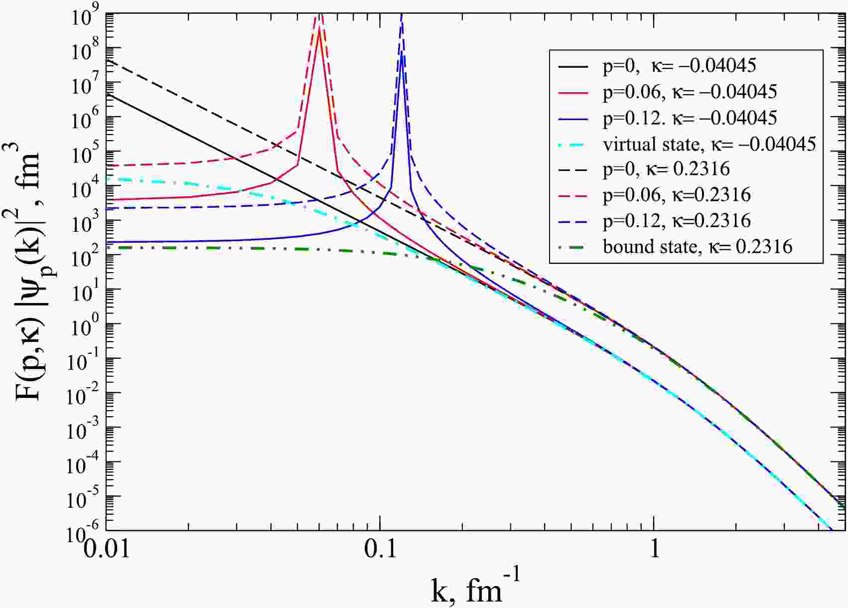
Let us now check the approximations (20) and (24). We use the Yamaguchi potential [26] with the parameter $ \beta = 1.4488 $ fm⁻¹ and two values of $ \varkappa $ corresponding to two main $ NN $-configurations (at $ \hbar^2/2\mu = 41.47 $ MeV fm$ ^{2} $): $ \varkappa = -0.04045 $ fm^-1, which corresponds to the singlet $ NN $-channel with a virtual state, and $ \varkappa = 0.2316 $ fm⁻¹, which gives a bound state with $ E_b = -2.2244 $ MeV.

Figure 1 shows the momentum distributions for the scattering wave functions $ \rho_p(k) = F(p, \varkappa)|\psi_p(k)|^2 $, calculated for the two above-mentioned values of $ \varkappa $ and three energies corresponding to the values of the on-shell momentum: $ p = $0, 0.06, and 0.12 fm^-1 in comparison with the momentum distributions for the virtual state $ |u_v(k)|^2 $ and bound state $ |u_b (k)|^2 $.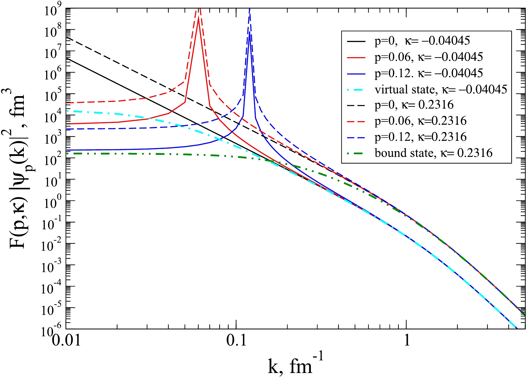

Figure 1.  (color online) Momentum distributions for the scattering functions $\rho_p(k)=F(p,\varkappa)|\psi_p(k)|^2$ for the Yamaguchi potential at three values $p=$0, 0.06, and 0.12 fm⁻¹ and for two values of $\varkappa$: -0.04045 fm⁻¹ (solid curves) and $\varkappa=0.2316$ fm⁻¹ (dashed curves) compared to the momentum distributions for the virtual state $|u_v(k)|^2$ and bound state $|u_b (k)|^2$.

As can be seen from Fig. 1, the momentum distributions $ \rho_p(k) = F(p, \varkappa)|\psi_p(k)|^2 $ found from the low-energy scattering wave functions do not depend on p at $ k>p $ and approach (in absolute value) the corresponding momentum distribution for the virtual or bound state. Thus, the approximation based on the Fäldt–Wilkin equality does indeed work in the region of large momenta for both the bound and virtual states. Note that, as discussed above, a chosen form of the virtual state wave function means that the integral $ \int_0^\infty|u_v(k)|^2k^2{\rm d}k $ is not equal to unity in contrast to the bound-state. For example, such an integral of $ |u_v(k)|^2 $ with $ \varkappa = -0.04045 $ fm^-1, as shown in Fig. 1, is equal to 0.8377.

To demonstrate the accuracy of the approximation (20), Fig. 2 shows the ratios of the momentum distributions $ \rho_p(k) $ at different p to the virtual-state momentum distribution $ \rho_v(k) $. This ratio has the form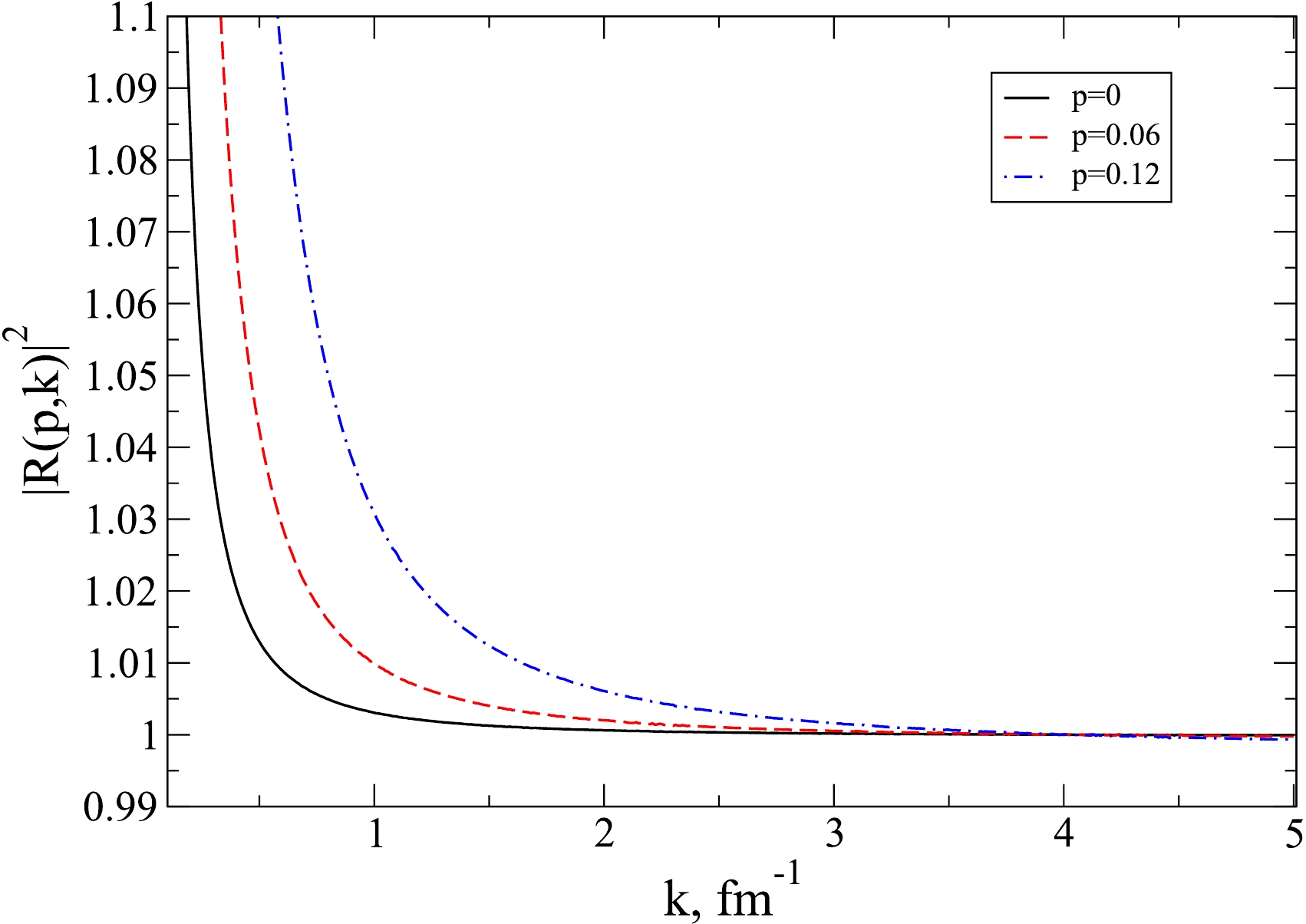

Figure 2.  (color online) Ratio of momentum distributions for the scattering functions $\rho_p(k)=F(p,\varkappa)|\psi_p(k)|^2$ at $p=$0, 0.06, and 0.12 fm⁻¹ to the distribution for the virtual state $|u_v(k)|^2$ at $\varkappa=0.04045$ fm⁻¹.

where the function determining k dependence

monotonically approaches 1 (the faster it does, the smaller $ \varkappa^2+p^2 $). At the same time, the ratio $ R_{p, \varkappa}(k) $ tends to the limit value $ A( \varkappa,p) $, which is slightly less than 1, even at zero energy $ p = 0 $, due to the non-zero value of $ \varkappa $.

The limit values $ A( \varkappa,p) $ for $ \varkappa = -0.0405 $ fm^-1 are 0.9998, 0.9994, and 0.9980 for $ p = 0 $, 0.06, and 0.12 fm^-1, respectively. For comparison, the limit ratio $ A( \varkappa,0) $ at $ \varkappa = 0.2316 $ fm^-1, corresponding to the bound state, is 0.9971. As can be seen from Fig. 2, at $ p = 0 $, the ratio $ R_{p, \varkappa}(k) $ differs from 1 by less than one percent for all $ k>0.6 $ fm^-1. The above accuracy of the approximation (20) seems to be sufficient for calculations with such two-nucleon momentum distributions.

Let us now test the approximations based on the Fäldt–Wilkin factor for a realistic local $ NN $ interaction. In Fig. 3, we present the momentum distributions for the $ ^1S_0 $ $ np $ scattering wave functions with the factor (21) at three values of energy for the Argonne V18 (AV18) potential [27]. Here, the wave number of the virtual state is $ \varkappa_{v} = -0.04 $ fm^-1. All three curves in this figure are almost indistinguishable in the region $ k>1 $ fm^-1. Thus, the FWF indeed allows us to get close momentum distributions at different small on-shell momenta. Based on the exact equality (17) and the results for separable interaction, we assume that the approximation (20) is also valid for realistic interaction. That is, the momentum distribution for the scattering state multiplied by the factor (21) is an approximation of the momentum distribution for the virtual state in this case.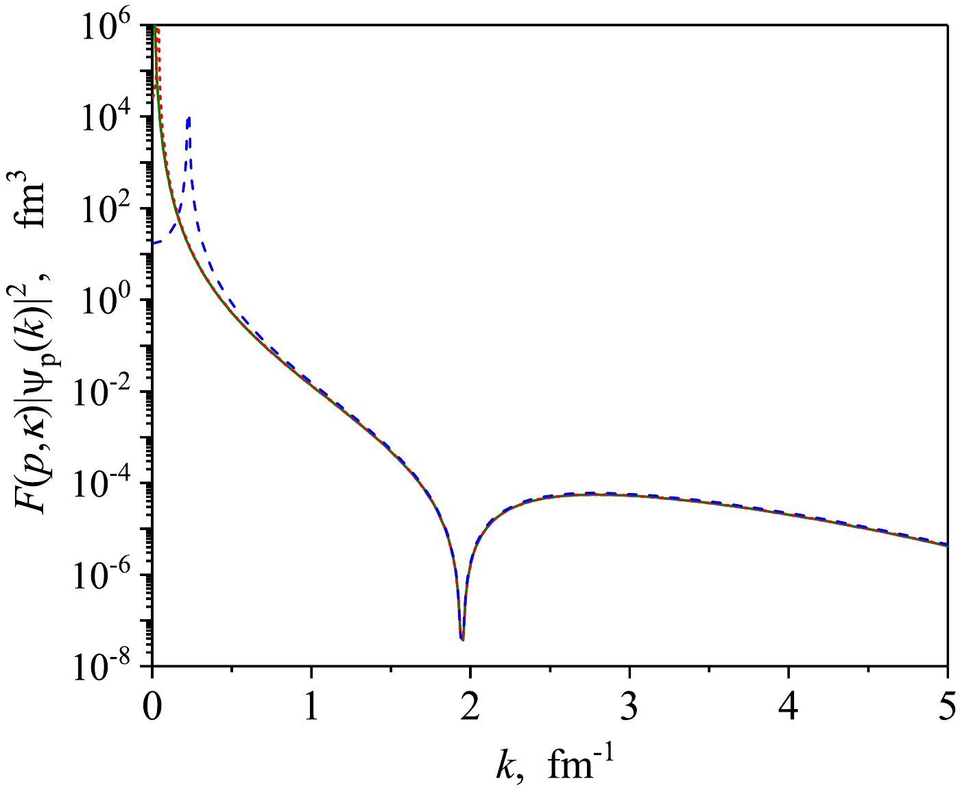

Figure 3.  (color online) Spin-singlet $np$ momentum distributions for the AV18 potential with the factor from Eq. (20) for three momenta: $p=0.008$ fm⁻¹ (solid curve), $p=0.041$ fm⁻¹ (dotted curve), and p=0.23 fm⁻¹ (dashed curve).

In Fig. 4, we test the relation (24) for the $ ^3S_1 $-$ ^3D_1 $ coupled channels with AV18 $ NN $ interaction. Here, $ \varkappa_d = 0.2316 $ fm^-1. Although all three curves are very close to each other in the high-k region, one can see a small deviation of the momentum distributions found from the scattering wave functions from the deuteron one, even for the smallest p. Thus, the approximate relation (24) is also valid for realistic $ NN $-interaction. Here, we can even estimate its error, which is approximately 5% for the case of zero energy.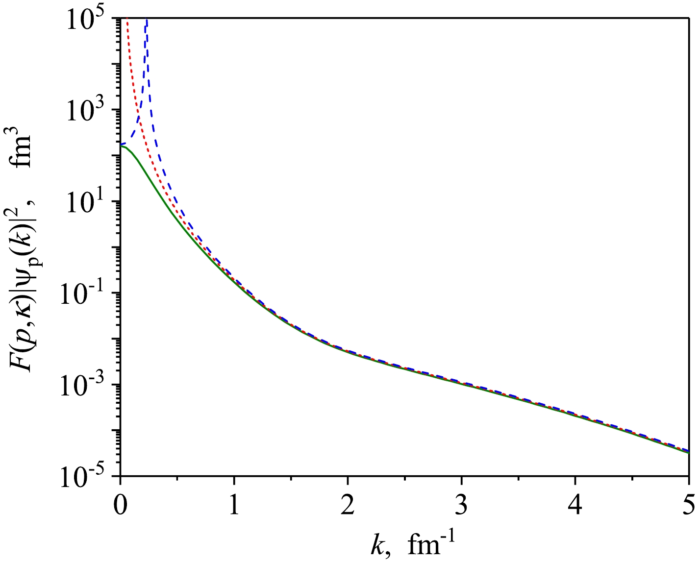

Figure 4.  (color online) Deuteron momentum distribution (solid curve) for AV18 potential in comparison with the momentum distributions found from the scattering wave functions according to Eq. (24): $p=0.041$ fm^-1 (dotted curve) and $p=0.23$ fm^-1 (dashed curve).

Taking into account the above example with a separable potential, it can be concluded that the FWF-based approximation works slightly better for the spin-singlet channel due to the smaller value of $ | \varkappa| $. Thus, the error for the spin-singlet channel should be no more than 2%−3%.

The results of the previous sections allow us to introduce a new form for UMD for the singlet $ NN $ channels based on the scattering wave functions at zero or small on-shell momentum p as follows:

Based on the results of the previous sections, in the high-momentum region, these distributions should approximate the momentum distribution for the virtual state (6) (whose wave function in the configuration space is uniquely determined by the ANC (5)):

Here, it should be noted that for the interactions that take the charge dependence of $ NN $ forces into account, one will have three different singlet UMDs for $ pp $, $ np $, and $ nn $ pairs. The values of $ \varkappa_v $ differ for these three cases as well.

The corresponding UMD for the spin-triplet channel is just the deuteron momentum distribution. A comparison of the deuteron momentum distributions for different $ NN $ interactions is presented in Fig. 5. Below, we consider four models for $ NN $ interactions: CD Bonn potential [28], AV18 potential [27] and two versions of the dibaryon model with energy dependent interactions, DBM-1 and DBM-2024 (see details and further Refs. in [29]). As shown in Fig. 5, the deuteron momentum distributions at small relative momenta are nearly indistinguishable for the considered interactions, while in the high-momentum region, at $ k>1.3 $ fm^-1, all distributions show quite different behavior. Thus, we chose the above interactions with evidently different high-momentum properties for further tests of the presented formalism.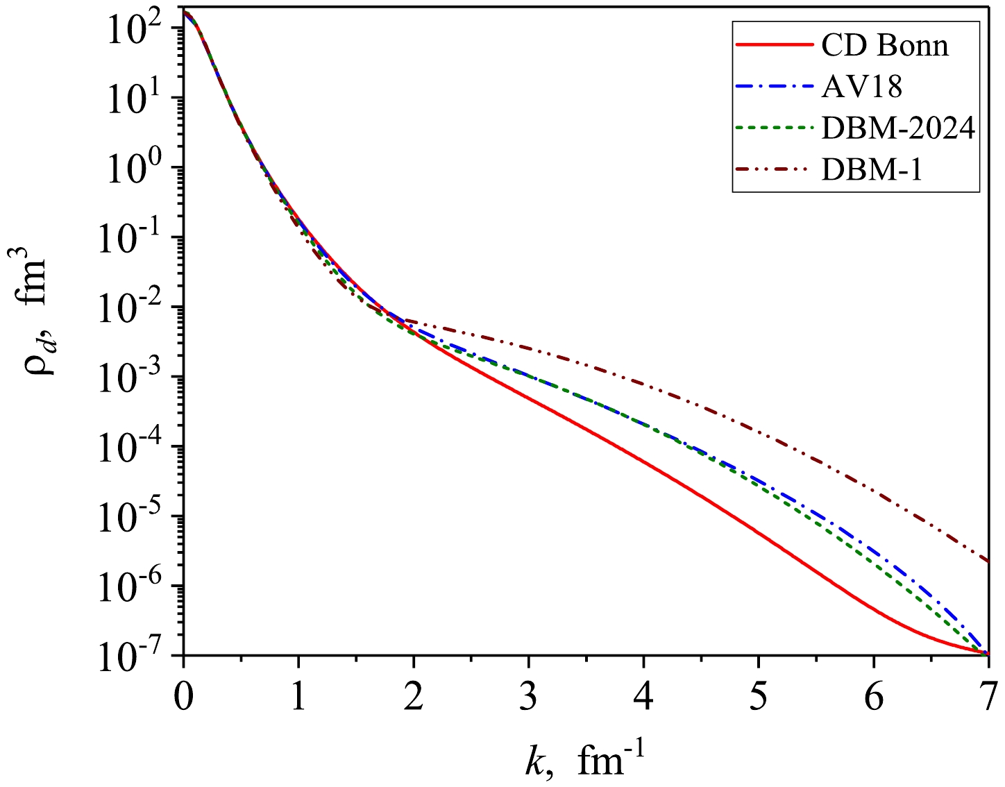

Figure 5.  (color online) Spin-triplet (deuteron) $np$-momentum distributions for different realistic $NN$-potentials: CD Bonn (solid curve), AV18 (dash-dotted curve), DBM-2024 (dashed curve), and DBM-1 (dash-dot-dotted curve).

A comparison of the spin-singlet $ np $ UMDs constructed from the scattering wave functions (calculated at $ p = 0.008 $ fm^-1) using (41) for the four above interactions is shown in Fig. 6.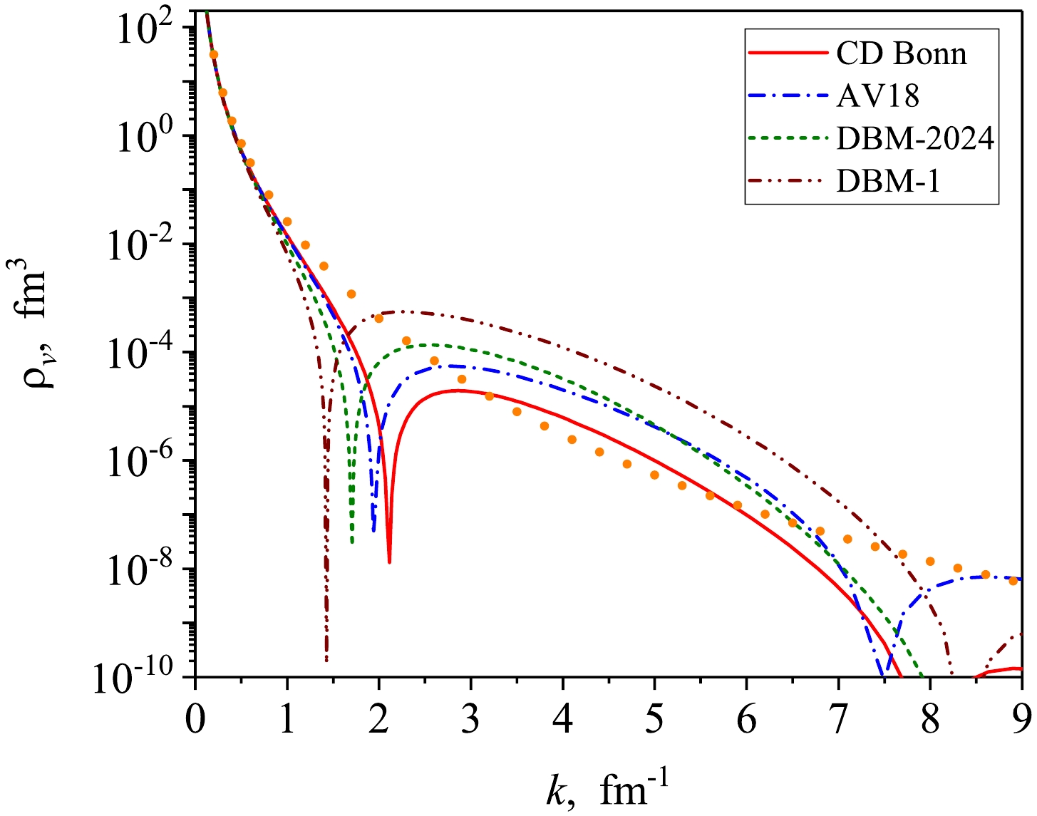

Figure 6.  (color online) Spin-singlet $np$ universal momentum distributions for different realistic $NN$-potentials. The notations are the same as in Fig. 5. The dots show the virtual-state momentum distribution for the Yamaguchi potential.

It can be seen that the UMDs for different interactions are almost the same in the momentum region $ 0.2<k<0.6 $ fm^-1. Also, in this region, they are close to the exact distribution $ \rho_v(k) $ for the separable Yamaguchi potential, as shown by dots. At the same time, at $ k >1 $ fm^-1, all distributions exhibit different behavior, which is primarily due to the difference in the position of the nodes of the corresponding wave functions.

Thus, by using the definition of (41), one can evidently compare high-momentum components of the distributions in the spin-singlet channels for different $ NN $ interactions. Below, we introduce constants that allow us to quantify these differences.

To consider high-momentum parts of the distributions, which just correspond to SRC, let us introduce the boundary of the high-momentum region as a constant $ p_0 $. Usually, it is taken to be comparable with the Fermi momentum $ k_F $ in nuclei [5, 13].

A high-momentum part of the deuteron (bound-state) distribution is defined by the integral

which, due to normalization to unity (2), is simply the weight of the high-momentum components in the deuteron. The values of $ a_2^d $ are different for different realistic $ NN $-interactions [13].

Now, one can consider the high-momentum parts of the singlet UMDs by taking the integral of the momentum distribution for the virtual state (6):

It should be emphasized that, unlike the triplet channel, the quantity $ a_2^v $ is not the weight of the high-momentum tail in the singlet channel. However, the quantity $ a_2^v $ is dimensionless, and its value estimates the high-momentum contribution for different $ NN $ interactions.

For practical calculation of these quantities, let us consider high-momentum integrals of the squared modulus of scattering wave functions:

where $ p\ll p_0 $ is assumed so that these integrals are finite. The functions $ c_2^{s(t)}(p) $ do not have the same meaning as the values $ a_2^d $ and $ a_2^v $, as is already evident from their dimension (fm$ ^{3} $); however, they contain quantitative information about the high-momentum components of the $ NN $ scattering states.

By using FWF, one can get an explicit approximate expression for the constant $ a_2^{v} $ for a virtual state:

The same approximate equality is also valid for the triplet channel, but there is no need for it there, as the high-momentum constant $ a_2^d $ is simply calculated from the deuteron momentum distribution.

To check the relation (46), Fig. 7 shows the function $ c_2^s(p)F(p, \varkappa_{np}) $ for the $ NN $ potentials considered here. As can be seen from the figure, these functions are practically constant at $ p<0.1 $ fm^-1, which allows us to calculate the values $ a_2^v $ for different potentials from the scattering wave functions.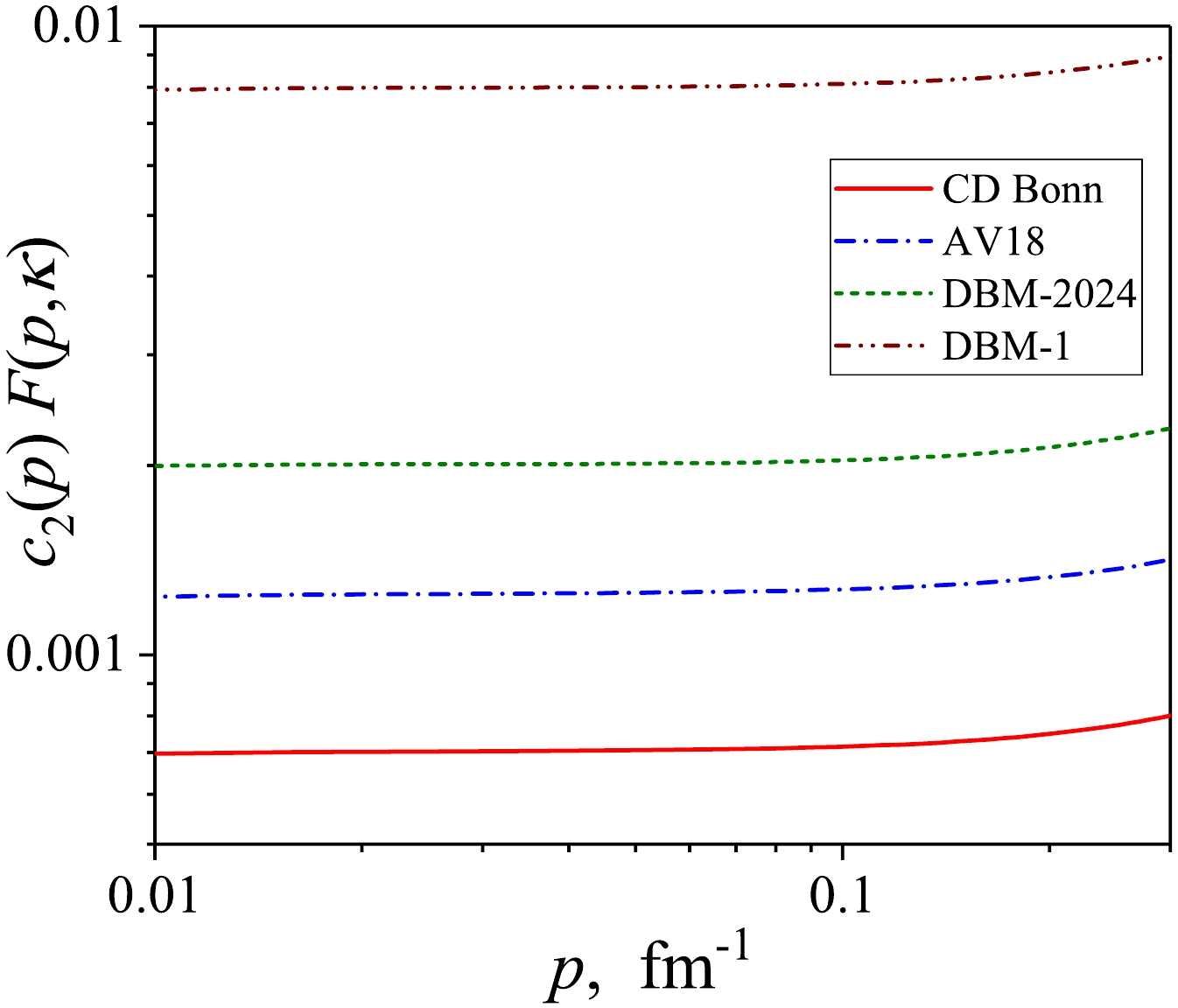

Figure 7.  (color online) Function $c_2^s(p)$ with the factor (21) at low on-shell momentum p for different $np$ potentials.

The values of $ a_2^v $ for different $ NN $ interactions in comparison with $ a_2^d $ found for the deuteron momentum distribution are given in Table 1. Here, the high-momentum region boundary $ p_0 = 1.4 $ fm^-1 is used, which corresponds to the generally accepted value of $ k_F $ for nuclei. From Table 1, it can be seen that the spread of high-momentum constants for various interactions is different for triplet and singlet channels. In all cases, even for the traditional AV18 and CD Bonn models, the $ a_2^{v} $ constants differ from each other more than the $ a_2^d $ constants for the same potentials.

model	$ a_2^d \qquad $	$ a^{v(np)}_2\qquad $	$ a^{v(pp)}_2 \qquad $	$ a_2^{v(pp)}/a_2^d $
CD Bonn	0.031	0.0007	0.0009	0.03
AV18	0.041	0.0013	0.0016	0.04
DBM-2024	0.036	0.002	0.0026	0.07
DBM-1	0.068	0.008	0.011	0.16

Table 1.  High-momentum constants for different $ NN $ models for $ p_0=1.4 $ fm^-1.

Note also that the $ a_2^d $ value for DBM-2024 is slightly smaller than that for AV18, while the $ a_2^v $ values are more than 1.5 times larger than for AV18. Thus, one can conclude that the value $ a_2^v $ represents an independent high-momentum characteristic of the $ NN $ interaction in spin-singlet channels.

In Table 1, the high-momentum constants for the $ pp $ interaction, $ a_2^{v(pp)} $, are also presented. These constants correspond ² to $ \varkappa_{pp}\approx - 0.054 $ fm^-1. It is clear that the ratio $ a_2^{v(pp)}/a_2^{v(np)} $ depends very weakly on the model.

Finally, in Table 1, we present the ratios of constants $ a_2^{v(pp)}/a_2^d $, which are discussed in the next subsection.

Recently [18], we proposed a way to calculate the weight of high-momentum components for scattering wave functions via the integral over on-shell momentum p up to some small value q ($ q\ll{p_0} $):

Such an integral is dimensionless and can be compared with the $ a_2^d $ value for the bound-state wave function.

Now, one can also quantitatively compare the weights of high-momentum components for the singlet and triplet channels using the ratio [18]

The values in the numerator and denominator represent the cumulative weights of high-momentum components from all states of the spectra up to the energy related to the considered on-shell momentum q in the singlet and the triplet $ NN $ channels, respectively.

Using the relations in (46) as approximations for both singlet and triplet functions $ c_2(p) $ at small values of p, one gets the following approximate expressions for the high-momentum integrals $ A(q) $ at small q:

This results in the following relation for the ratio $ \eta(q) $:

A useful feature of this presentation is that the function ζ depends on the on-shell parameters $ \varkappa_v $ and $ \varkappa_d $ only, so the dependence on q in the ratio η is the same for all the realistic $ NN $ interactions. Thus, the only difference in the values of $ \eta(q) $ for different $ NN $ interaction models is the ratio of the constants $ a_2^v/a_2^d $. At $ q = | \varkappa_{pp}| $ and $ q = \varkappa_d $, the corresponding ratios are as follows:

One can see that the ratio of high-momentum weights $ \eta(q) $ increases with increasing q, showing that the spin-singlet channel contribution to high-momentum components grows faster with energy than the spin-triplet one. At the same time, the ratio $ a_2^{v(pp)}/a_2^d $ represents an informative characteristic for high-momentum components of the momentum distributions in continuum for the chosen model of the $ NN $ interaction.

Using the data from Table 1, one can compare the ratios $ a_2^{v(pp)}/a_2^d $ at $ p_0 = 1.4 $ fm^-1 for different $ NN $ interactions. From the considered models, the minimal value of this ratio corresponds to the CD Bonn potential, while the DBM-1 gives an essentially greater one. Based on the contact formalism, we may also expect that the use of an interaction with greater $ a_2^v/a_2^d $ ratio at the two-nucleon level will lead to greater mean values for the ratios of $ pp $ and $ np $ momentum distributions in nuclei.

Figure 8 presents the ratio $ a_2^{v(pp)}/a_2^d $ as a function of the high-momentum parameter $ p_0 $. One can see that the ratio $ a_2^{v(pp)}/a_2^d $ depends significantly on the value of $ p_0 $. It is interesting to note that the minimum of this ratio for the conventional AV18 and CD Bonn potentials corresponds just to the most frequently considered range of $ p_0 \sim 1.3-1.5 $ fm^-1, where the pp/np ratio is very sensitive to the chosen value of $ p_0 $.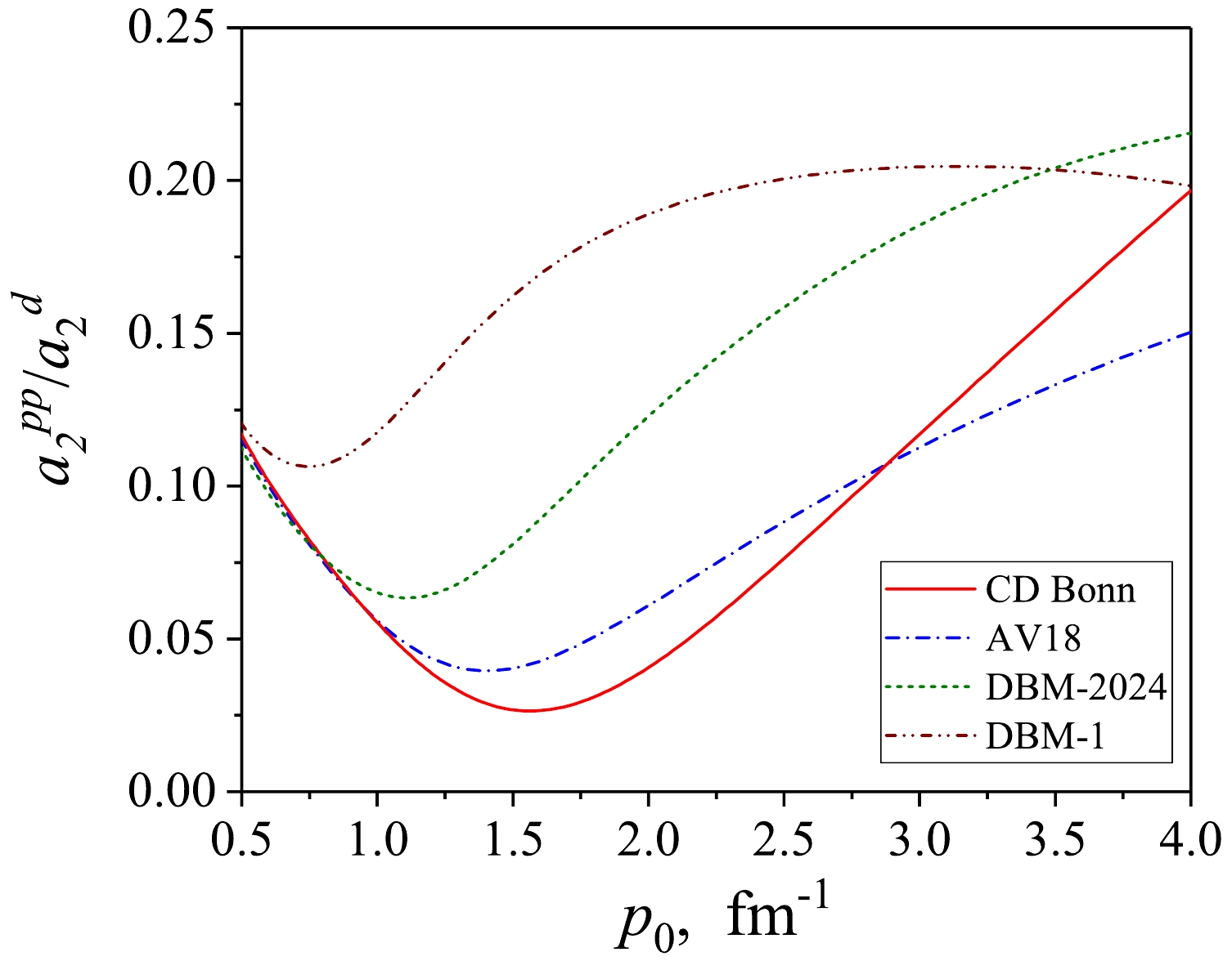

Figure 8.  (color online) Ratio of $a_2^{v(pp)}/a_2^d$ values as a function of high-momentum parameter $p_0$ for different $NN$ potentials.

Thus, the UMDs suggested in this section are quite convenient for practical calculations. The developed formalism also allows a high-momentum constant $ a_2^v $ to be introduced for the spin-singlet channel, in addition to $ a_2^d $ for the deuteron channel. Besides, some estimations for the ratios of $ pp $ and $ np $ momentum distributions in nuclei for various models of $ NN $ interactions can already be given at the two-body level. In the next section, we show how the introduced UMDs can be employed within the contact formalism for analyzing $ NN $ distributions in $ ^3 {\rm{He}}$.

Here, we test the factorization property (1) of two-nucleon momentum distributions $ \rho^A_{ { {NN}}} $ for the$ ^3 {\rm{He}}$ nucleus as an example and calculate the nuclear contacts $ C^{^3{\rm He}}_{ { {NN}}} $ for various interactions. We consider the distributions $ \rho^A_{ { {NN}}}(k,Q = 0) $, which correspond just to back-to-back SRC pairs, where Q is the center-of-mass momentum of the pair.

In this case, it is convenient to introduce the normalized distribution at $ Q = 0 $ as follows [9]:

where $ n_{ { {NN}}} $ is a number of nucleon pairs, which is equal to 2 for $ NN = np $ and 1 for $ NN = pp $. Note that with such a normalization, the distribution of the center-of-mass momentum of a pair of nucleons $ \rho^{A, { {NN}}}_{\rm{cm}}(Q) $ is assumed to be normalized to 1.

According to [9], the normalized momentum distribution is proportional to the UMD $ \rho_{ { {NN}}}(k) $ in the high-momentum region, with the nuclear contact as a factor:

Here, because we consider only the $ ^3 {\rm{He}}$ nucleus, we have omitted the index A, indicating the nucleus, in the notations of the distributions ρ and nuclear contacts C. Below, we use the UMDs $ \rho_{np} = \rho_d $ and $ \rho_{pp} = \rho_{v(pp)} $ for $ np $- and $ pp $-pairs, respectively.

We use the same four $ NN $ interactions: CD Bonn, AV18, DBM-1, and DBM-2024 listed in the previous section and the $ ^3 {\rm{He}}$ $ NN $-distributions calculated using these interactions and corresponding three-particle forces. The $ ^3 {\rm{He}}$ distributions for AV18 potential with UIX $ 3N $ force are taken from Ref. [30], the distributions for CD Bonn potential supplemented with $ 3N $ TM force are from Ref. [13], and the distributions for the two versions of the DBM were obtained by the present authors from the variational calculations on an antisymmetrized Gaussian basis (see details in Ref. [29]).

First, let us check how the factorization (53) is satisfied for $ np $ distributions, where the momentum distribution in the deuteron is used as the UMD. Figure 9 shows the normalized momentum $ np $-distributions in $ ^3 {\rm{He}}$ at $ Q = 0 $, $ \rho^0_{np}(k) $, for the different interaction models in comparison with the corresponding deuteron distributions $ \rho_d(k) $ multiplied by the corresponding nuclear contacts $ C_{np} $.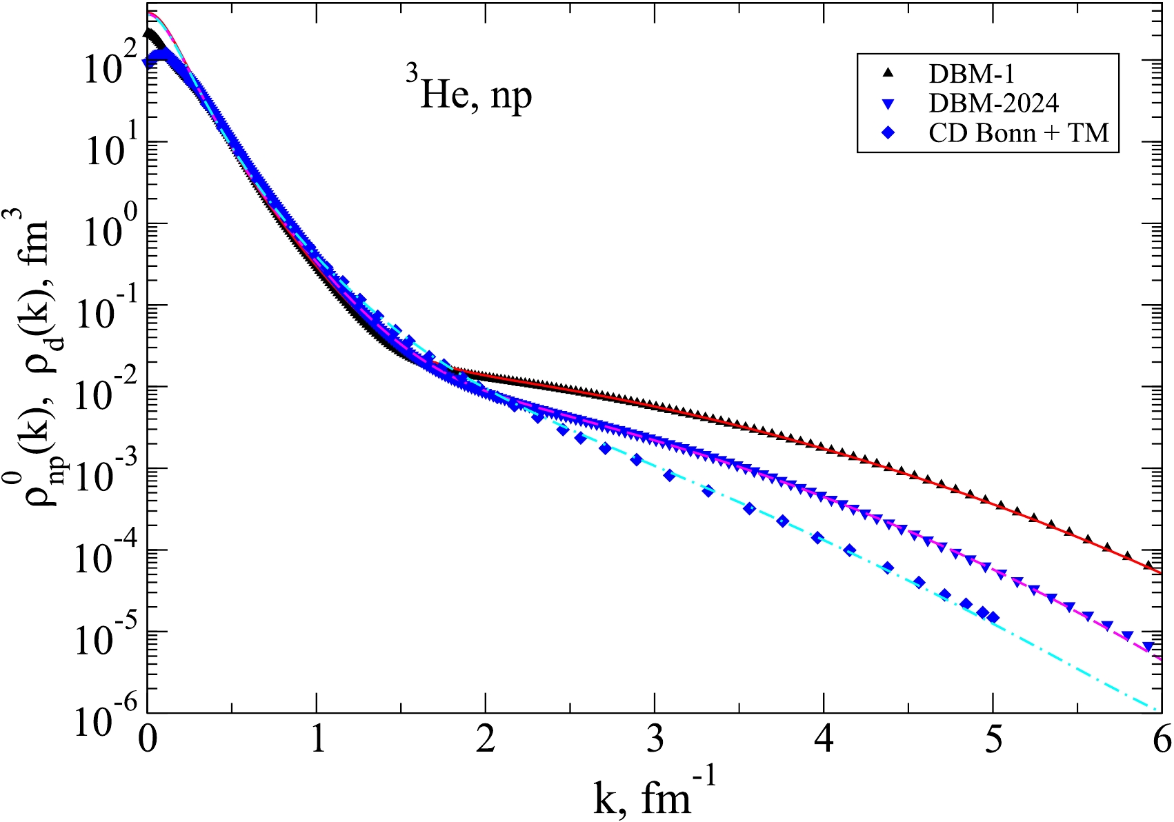

Figure 9.  (color online) Normalized momentum $np$-distributions in $^3$He at $Q=0$, $\rho^0_{np}(k)$, for three interaction models (DBM-1 – triangles-up, DBM-2024 – triangles-down, CD Bonn+TM – diamonds) in comparison with the corresponding deuteron distributions $\rho_d(k)$ multiplied by $C_{np}$ (solid curves).

Here, for all the interaction models considered, the $ ^3 {\rm{He}}$ momentum distributions achieve the deuteron "asymptotics" already at the relative momentum $ k \sim 1.5 $ fm^-1. Although high-momentum parts of the distributions for different interactions differ significantly, their ratios to their "own" deuteron momentum distributions in the high-momentum region (i.e., the nuclear contacts) are nearly independent of the interaction model. The found nuclear contacts $ C_{np} $ for all considered interaction models are close to 2, which agrees with the results of Ref. [9]. The values of $ C_{np} $ found in the present study are given in Table 2.

	AV18 + UIX	CD Bonn + TMa	DBM-1	DBM-2024
$ C_{np} $	$ 1.82\pm 0.07 $	2.2	$ 2.26\pm 0.03 $	$ 2.17\pm 0.04 $
$ C_{pp} $	$ 2.91\pm 0.16 $	3.1	$ 3.12\pm 0.03 $	$ 2.98\pm 0.05 $
aThe data on the distribution in $ ^3 {\rm{He}}$ are obtained by digitizing the figure in Ref. [13] so that the results are given without errors.

Table 2.  Nuclear contacts for $ ^3 {\rm{He}}$ for different models of $ NN $ and $ 3N $ interaction.

Now, having the UMD for the singlet channel $ \rho_v(k) $, one can compare the normalized momentum $ pp $-distributions in $ ^3 {\rm{He}}$ at $ Q = 0 $ with these UMDs and find the corresponding nuclear contacts $ C_{pp} $. Figure 10 shows such a comparison for the four interaction models considered. Here, the ratios of the $ pp $-distributions to the corresponding UMDs become nearly constant at values of $ k\geq 2.3 $ fm^-1. In this figure, we show the UMDs multiplied by the corresponding nuclear contacts $ C_{pp} $, the values of which are given in Table 2 and are close to 3.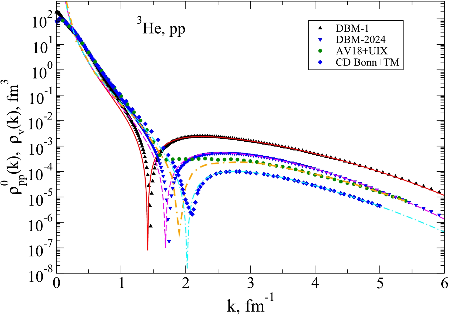

Figure 10.  (color online) Normalized momentum $pp$ distributions in $^3$He at $Q=0$, $\rho^0_{pp}(k)$, for four interaction models in comparison with the corresponding singlet UMDs, multiplied by the contacts $C_{pp}$. The notations are the same as in Fig. 9, with filled circles representing AV18+UIX.

As mentioned above, the values of the nuclear contacts found for the $ np $-pairs are consistent with the results of Ref. [9]. However, these values of both $ np $- and $ pp $-nuclear contacts differ from those given in Ref. [5] because the definitions of the corresponding UMDs and nuclear contacts are different there ³ (see also the relations between momentum distributions in Appendix A).

Thus, we have shown that the nuclear contacts for the $ ^3 {\rm{He}}$ nucleus, calculated with respect to the two-particle UMD corresponding to a virtual state, are indeed almost identical for $ NN $ interactions; nevertheless, the high-momentum components of the momentum distributions for those interactions differ significantly at $ k>p_0 $. Based on the results of the contact formalisms [5, 9], one may expect that this property will hold for heavier nuclei.

In this paper, we have suggested a way to construct the momentum distributions for the spin-singlet $ ^1S_0 $ $ NN $ channels based on the virtual state from the low-energy scattering wave functions. The advantages of such momentum distributions are as follows:

$ ({\rm{i}}) $ The distribution does not depend on the boundary of the high-momentum region $ p_0 $.

$ ({\rm{ii}}) $ One can introduce two-nucleon short-range constants $ a_2^v $ for spin-singlet channels, which characterize the $ NN $ interaction with respect to high-momentum components of wave functions, similar to the value $ a_2^d $, which is well known for the deuteron channel.

$ ({\rm{iii}}) $ The ratio $ a_2^{v(pp)}/a_2^d $ differs for various realistic $ NN $ models and allows us to estimate differences in ratios of $ pp $- and $ np $-momentum distributions in nuclei.

$ ({\rm{iv}}) $ In the low-momentum region, the momentum distribution for the virtual state depends only on the on-shell characteristics of the $ NN $-system, such as the wave number $ \varkappa $ and scattering length, which are the same for all realistic $ NN $ interaction models. Thus, the introduced UMDs turn out to be the same for different models in the momentum region of 0.2−0.6 fm⁻¹, exhibiting obvious differences at high momenta.

$ ({\rm{v}}) $ Due to the previous property, the nuclear contacts calculated relative to the introduced UMDs should be nearly the same for different realistic $ NN $ interactions.

The last property has been demonstrated for $ A = 3 $ nuclei with four essentially different models of $ NN $ interactions, which correspond to the same observables in $ 2N $ and $ 3N $ systems. One can expect that a weak dependence of nuclear contacts on the $ NN $ interaction will also hold for heavier nuclei, which should be studied and verified in future research.

The above conclusion seems to differ from the results of Ref. [5], where a spread of the $ pp $-nuclear contacts for different $ NN $ interactions was found. This is caused by the difference in the definitions of UMDs and nuclear contacts. At the same time, the relation (A5) from Appendix A shows that the ratio of nuclear contacts for two nuclei remains the same for differently defined UMDs. This result agrees with the findings of Ref. [5], where a very weak dependence on the interaction models for such ratios of the nuclear contacts was demonstrated.

The suggested spin-singlet universal distributions based on the momentum distribution for the virtual state can be considered as a supplement to the contact formalism presented in Ref. [9] for the triplet $ np $ distributions. Because the proposed UMDs do not depend on the high-momentum boundary $ p_0 $, one can expect that our formalism will be suitable for calculations with $ NN $ models using various "low-k" approximations. In particular, the nuclear $ pp $-contacts for such interactions would be the same as for other realistic $ NN $ models, as the momentum distributions for the virtual state are nearly identical at low momenta for all realistic $ NN $ interactions. One may assume that the contacts will not depend on the cut-off parameters for this type of $ NN $ potentials as well.

Let us show how the introduced UMDs are related to other universal distributions used in the GCF.

The momentum distribution for the virtual state can be calculated using the scattering wave function at zero energy $ \psi_{p = 0}^s(k) $ (normalized according to (7)) from the relation

which is valid with high accuracy at $ k>0.5 $ fm⁻¹.

The universal momentum distributions normalized to unity in the region $ [p_0,\infty) $ can be calculated from the ratios [18]

where functions $ c_2(p) $ are defined in Eq. (45). It has been shown [18] that these distributions do not depend on p in the high-momentum region.

Thus, by using Eq. (46) for the spin-singlet channel, one gets that such a "tail-normalized" distribution is related to the density defined in Eq. (41) as follows:

which can be used at $ p = 0 $ as well. At the same time, the nuclear contacts defined relatively these two types of the universal distributions are recalculated as follows:

where $ \bar{C}_{pp}^A $ is a nuclear contact corresponding to the distribution $ \bar{\rho} $. This property shows that the ratios of the nuclear contacts for two nuclei $ A_1 $ and $ A_2 $ are the same for both distributions: