


 Abstract
 HTML
 Reference
 Related
 PDF


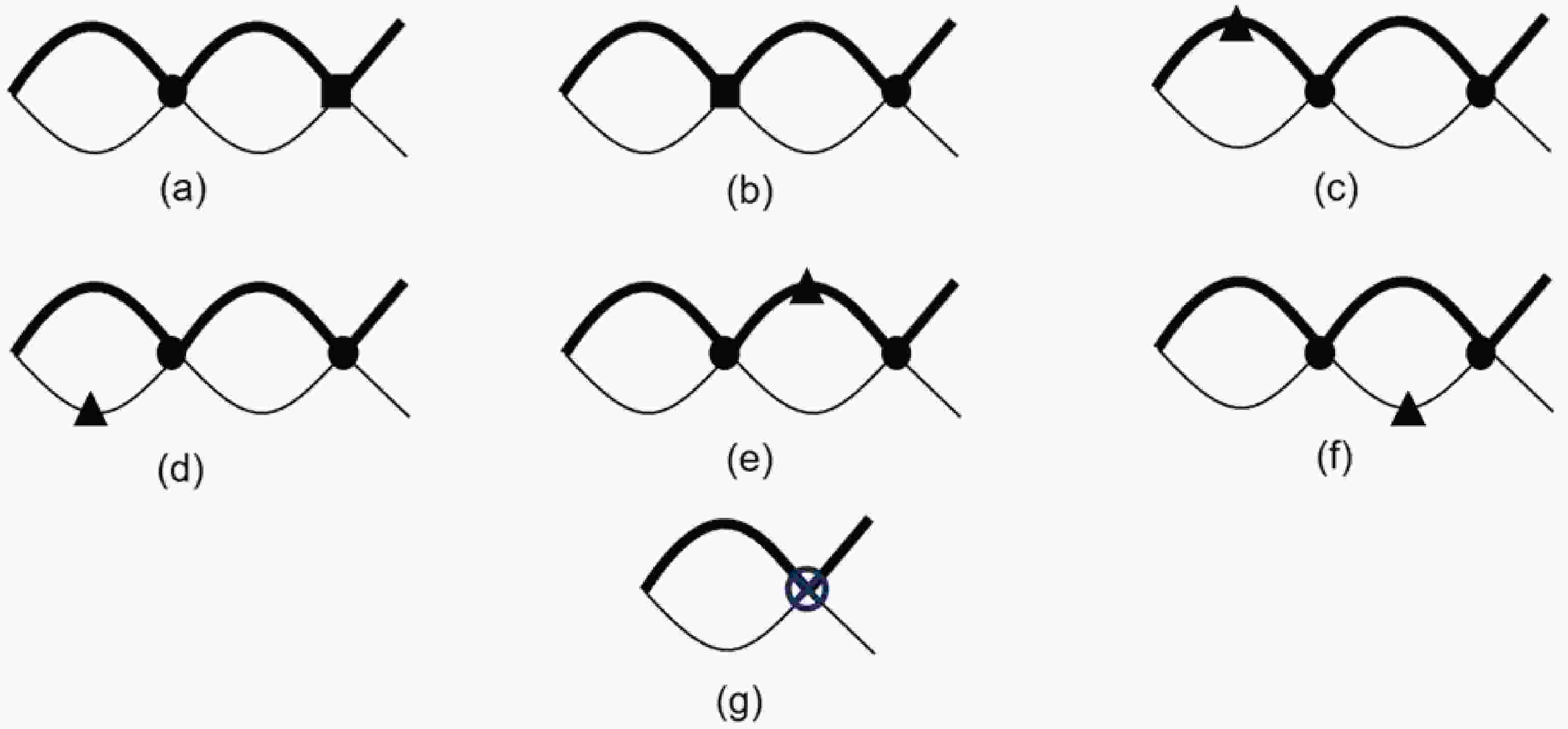


-
The
$ B_c $ meson is the only ground-state meson in the Standard Model composed of two heavy quarks of distinct flavors. In this work, we adopt the convention$ B_c^+(\bar b c) $ , with the charge-conjugate channel implied throughout. Unlike flavor-neutral quarkonia, such as charmonium and bottomonium, the$ B_c $ possesses open bottom and charm quantum numbers and therefore decays exclusively via weak interactions. This distinctive property gives the$ B_c $ a relatively long lifetime,$ \tau_{B_c}\approx0.51\; {\rm{ps}} $ [1, 2], making it a valuable system for precision studies of QCD and weak interactions.The
$ B_c $ meson was first observed by the CDF Collaboration in 1998 in$ p\bar p $ collisions at$ \sqrt{s}=1.8\; {\rm{TeV}} $ through the semileptonic decay channel$ B_c^\pm\to J/\psi\,\ell^\pm\nu $ [3]. Subsequent measurements at the Tevatron and the LHC have refined its mass, lifetime, and production properties [1, 2]. The spectroscopy of excited$ B_c $ states has also seen substantial progress: the ATLAS Collaboration reported evidence for the$ B_c(2S) $ state in 2014 [4], and both CMS and LHCb later observed the$ B_c(2S) $ and$ B_c^*(2S) $ states [5, 6]. The ground-state vector meson$ B_c^*(1S) $ , however, has not yet been observed, primarily because it is expected to decay predominantly through the radiative transition$ B_c^*\to B_c\gamma $ , with a soft photon that poses significant experimental reconstruction challenges. The hyperfine splitting between the$ B_c $ and$ B_c^* $ is predicted to lie in the range$ 60 $ –$ 70\; {\rm{MeV}} $ [7, 8].The doubly heavy structure of the
$ B_c $ system permits a clean separation between perturbative dynamics at the heavy-quark mass scale and nonperturbative bound-state effects. In the NRQCD factorization approach [9], the decay constants can be expressed as products of perturbatively calculable short-distance coefficients (SDCs) and universal long-distance matrix elements (LDMEs). The pseudoscalar decay constant$ f_{B_c} $ governs the purely leptonic decay$ B_c\to\ell\nu_\ell $ and enters the determination of the CKM matrix element$ |V_{cb}| $ [10, 11]. It is also relevant to precision flavor tests and searches for new physics beyond the Standard Model [12]. The vector decay constant$ f_{B_c^*} $ plays the corresponding role for the vector meson$ B_c^* $ .Considerable effort has been devoted to higher-order QCD corrections to these decay constants. The one-loop QCD correction to
$ f_{B_c} $ was obtained by Braaten and Fleming [10]. An important step toward the full higher-order result was taken by Onishchenko and Veretin, who computed the two-loop short-distance coefficient as an asymptotic expansion in the small mass ratio$ m_c/m_b $ [13]. Later, Chen and Qiao derived the complete two-loop result for an arbitrary mass ratio [11], and the pseudoscalar coefficient is now known numerically through three loops [14]. For the vector channel, the NNLO matching coefficient was obtained in Ref. [15], and the$ B_c^* $ decay constant was subsequently evaluated through$ {\cal{O}}(\alpha_s^3) $ [16]. Three-loop matching coefficients are also available for a broad set of heavy flavor-changing currents [17, 18]. These studies indicate that large corrections to the matching coefficients can be partially compensated by corrections to the wave functions at the origin when the scale relations of potential NRQCD are employed [17]. Complementary determinations from QCD sum rules and lattice QCD can be found in Refs. [19, 20].The mode separation adopted in this work is based on the threshold expansion, also known as the method of regions [21]. Near a heavy-particle threshold, a loop momentum in QCD receives distinct homogeneous contributions from the hard, soft, potential, and ultrasoft regions. Taylor expansion of the integrand in each region yields the velocity expansion, while dimensional regularization avoids double counting through scaleless overlap integrals. Integrating out the hard region yields NRQCD; retaining separate dynamical degrees of freedom for the remaining regions gives rise to velocity NRQCD (vNRQCD) [22−27].
vNRQCD separates the soft three-momentum scale from the ultrasoft kinetic-energy scale and correlates their renormalization through the velocity renormalization group (VRG). Its label formalism provides a homogeneous velocity expansion in dimensional regularization, makes the pull-up mechanism for mixed soft-ultrasoft counterterms explicit, and supplies the natural framework for evolving the subtraction velocity from
$ \nu=1 $ to$ \nu\sim v $ [22, 26, 28]. The framework has passed nontrivial checks in threshold-current evolution, the running of the QCD potential through order$ v^2 $ , and ultrasoft-induced operator mixing [22−24, 26, 27, 29].For the equal-mass case, the two-loop scale dependence of the currents has long been established within the vNRQCD framework. The first rigorous derivation was carried out by Luke and collaborators [22], who performed a complete analysis for the
$ J/\psi $ channel. In this work, we extend this line of analysis to the unequal-mass sector. Our calculation provides a direct two-loop determination of the anomalous dimension for the flavor-changing currents and treats the pseudoscalar and vector channels1 on an equal footing through a spin-unified formalism.Our calculation concerns the two leading S-wave flavor-changing currents,
$ \chi_b^\dagger\psi_c $ and$ \chi_b^\dagger{\boldsymbol{\sigma}}\psi_c $ , which correspond to the pseudoscalar and vector channels, respectively. We determine their anomalous dimensions directly from the ultraviolet poles of the effective-theory current matrix elements. The advance is methodological: a direct, spin-unified vNRQCD derivation of coefficients previously known from full-QCD matching. The result is a compact analytical formula valid for an arbitrary mass ratio$ x=m_c/m_b $ . In the equal-mass limit$ x\to1 $ , our result reduces to the known quarkonium expressions, providing a robust consistency check of the calculation.Two related RG problems enter the analysis. Substituting the potential matching coefficients at
$ \nu=1 $ into the ultraviolet counterterm determines the fixed-order anomalous dimension of the standard NRQCD factorization-scale RGE; this quantity cancels the residual infrared poles in the full-QCD short-distance coefficients. The velocity renormalization group (VRG) correlates the soft and ultrasoft subtraction scales below$ \nu=1 $ and involves running potentials generated by soft-loop contractions and ultrasoft-induced mixing operators. The present work determines the current anomalous dimension and identifies the relevant unequal-mass mixing structure, while a full solution of the unequal-mass VRG remains a natural next step.The remainder of this paper is organized as follows. In Sec. II, we extract the relevant mode content of vNRQCD from the threshold expansion and present the ultrasoft, potential, and soft sectors of the effective Lagrangian. Section III is devoted to the definition of the bare currents and their renormalization constants; we then evaluate the ultraviolet poles from potential-loop contributions and derive the two-loop anomalous dimensions. The factorization-scale evolution of the leading LDME is illustrated in Sec. IV, and we conclude with a brief summary of our findings in Sec. V.
-
The method of regions determines the mode content of vNRQCD. Let p denote the magnitude of the relative three-momentum of the
$ c\bar b $ pair, and let$ E\sim \frac{p^2}{2m} $ denote its nonrelativistic energy. Near threshold, the relevant homogeneous momentum regions are [21]$ \begin{array}{l} \quad\quad \text{hard:}\quad k^0,|{\bf{k}}|\sim m_c\ \text{or}\ m_b, \\ \quad\quad\ \ \text{soft:}\quad k^0,|{\bf{k}}|\sim p, \\ \text{potential:}\quad k^0\sim E,\qquad |{\bf{k}}|\sim p, \\ \text{ultrasoft:}\quad k^0,|{\bf{k}}|\sim E. \end{array} $
(1) The familiar notation
$ p\sim mv $ and$ E\sim mv^2 $ provides a shorthand for these scalings. In the unequal-mass calculation below, the two kinetic energies and all subleading mass factors are kept distinct.The threshold expansion is obtained by Taylor expanding each QCD integrand according to the scaling rules in Eq. (1) and integrating each expanded term over the full loop-momentum domain. In dimensional regularization, overlap contributions are scaleless. The hard region is absorbed into the Wilson coefficients when QCD is matched onto the nonrelativistic effective theory. Potential modes describe the heavy constituents, soft modes transfer momenta of order p, and ultrasoft modes carry the kinetic energy E. vNRQCD makes the homogeneous scaling of these low-energy regions explicit in a mass-independent subtraction scheme through separate fields [22, 28].
-
In the
$ c\bar b $ center-of-mass frame, the potential fields carry soft three-momentum labels of equal magnitude and opposite sign:$ p_c^\mu =(m_c,{\bf{p}})+k_c^\mu, \ \ \ \ \ \ \ \ \ \ \ \ \ \ \ \ \ \ \ \ p_{\bar b}^\mu =(m_b,-{\bf{p}})+k_{\bar b}^\mu, $
(2) where
$ |{\bf{p}}|\sim p $ and$ k_c^\mu,k_{\bar b}^\mu\sim E $ . We denote the corresponding fields by$ \psi_{{\bf{p}}}(x) $ and$ \chi_{-{\bf{p}}}(x) $ . Their coordinate dependence contains residual ultrasoft momenta,$ i\partial^\mu\psi_{{\bf{p}}}(x)\sim E\,\psi_{{\bf{p}}}(x), \qquad i\partial^\mu\chi_{-{\bf{p}}}(x)\sim E\,\chi_{-{\bf{p}}}(x). $
(3) Soft gauge fields, light-quark fields, and ghost fields depend on both a soft label and residual coordinates. For example,
$ A_s^\mu(x)=\sum\limits_q e^{-iq\cdot x}A_q^\mu(x), \qquad q^\mu\sim p,\qquad i\partial^\mu A_q^\nu(x)\sim E\,A_q^\nu(x), $
(4) with analogous decompositions for
$ \varphi_q $ and$ c_q $ . Thus, the continuous coordinate labels the residual ultrasoft momentum, whereas the order-p soft momentum is discrete. Ultrasoft fields$ A_u^\mu(x) $ remain unlabeled.The vNRQCD Lagrangian is organized as
$ {\cal{L}}_{\rm{vNRQCD}}={\cal{L}}_u+{\cal{L}}_p+{\cal{L}}_s, $
(5) where the three terms correspond to ultrasoft interactions, four-fermion potentials, and soft interactions, respectively. At the order required here, the ultrasoft sector is
$\begin{aligned}[b] {\cal{L}}_u=\;&\sum\limits_{{\bf{p}}}\psi_{{\bf{p}}}^\dagger \left[ iD^0-\frac{({\bf{p}}-i{\bf{D}})^2}{2m_c} +\frac{{\bf{p}}^4}{8m_c^3} \right]\psi_{{\bf{p}}} \\& +\sum\limits_{{\bf{p}}}\chi_{-{\bf{p}}}^\dagger \left[ iD^0-\frac{(-{\bf{p}}-i{\bf{D}})^2}{2m_b} +\frac{{\bf{p}}^4}{8m_b^3} \right]\chi_{-{\bf{p}}}\\&-\frac14F_{u\,\mu\nu}^AF_u^{A\mu\nu}+\cdots . \end{aligned}$
(6) Here,
$ D^\mu $ contains the ultrasoft gauge field, and the antiquark transforms with$ \bar T^A=-(T^A)^* $ . Reparameterization invariance requires the label and residual derivatives to appear in the combinations shown in Eq. (6).The potential sector takes the form
$ {\cal{L}}_p=-\sum\limits_{{\bf{p}},{\bf{p}}'} V({\bf{p}},{\bf{p}}')\, \psi_{{\bf{p}}'}^\dagger\psi_{{\bf{p}}}\, \chi_{-{\bf{p}}'}^\dagger\chi_{-{\bf{p}}}. $
(7) For a
$ c\bar b $ system with unequal masses, the potential in the color basis used below can be expressed as [24, 26]$ \begin{aligned}[b]V({\bf{p}},{\bf{p}}') =\;& \left(T^A\otimes \bar T^A\right) \Bigg[ \frac{V_c^{(T)}}{{\bf{k}}^2} + \frac{V_k^{(T)}\pi^2}{2m_r|{\bf{k}}|} +\frac{V_2^{(T)}}{m_r^2}\\&- \frac{V_{2o}^{(T)}(m_b-m_c)^2}{8m_b^2m_c^2} + \frac{V_r^{(T)}({\bf{p}}^2+{\bf{p}}'^2)}{2m_bm_c\,{\bf{k}}^2} \\ & +\frac{V_s^{(T)}}{m_bm_c}{\bf{S}}^2 +V_\Lambda^{(T)}\Lambda({\bf{p}}',{\bf{p}}) +\frac{V_t^{(T)}}{m_bm_c}T({\bf{k}}) \Bigg], \end{aligned} $
(8) where
$ {\bf{k}}={\bf{p}}'-{\bf{p}} $ ,$ m_r=m_bm_c/(m_b+m_c) $ , and$ {\bf{S}}=({\boldsymbol{\sigma}}_1+{\boldsymbol{\sigma}}_2)/2 $ . Here,$ {\boldsymbol{\sigma}}_1 $ acts on the$ \bar b $ line and$ {\boldsymbol{\sigma}}_2 $ on the c line. The identity$ {\bf{S}}^2=\dfrac32\,{\bf{1}}+ \dfrac12\,{\boldsymbol{\sigma}}_1 \cdot {\boldsymbol{\sigma}}_2 $ relates the total-spin and spin–spin bases. Expressing$ V_s^{(T)}{\bf{S}}^2/(m_bm_c) $ in the latter basis yields the spin-independent contact term$ 3V_s^{(T)}/(2m_bm_c) $ together with the spin–spin term. Throughout, we retain the$ {\bf{S}}^2 $ basis and include this contact term in$ V_s^{(T)} $ . The remaining spin-dependent structures are defined by$ \begin{aligned}[b]\Lambda(\mathbf{p}',\mathbf{p})=\;& i\frac{{\boldsymbol{\sigma}}_1\cdot(\mathbf{p}'\times \mathbf{p})}{2\mathbf{k}^2m_b} \left(\frac{1}{2m_b}+\frac{1}{m_c}\right) \\&+i\frac{{\boldsymbol{\sigma}}_2\cdot(\mathbf{p}'\times \mathbf{p})}{2\mathbf{k}^2m_c} \left(\frac{1}{2m_c}+\frac{1}{m_b}\right),\end{aligned} $
(9) $ T(\mathbf{k})={\boldsymbol{\sigma}}_1 \cdot {\boldsymbol{\sigma}}_2 -\frac{3(\mathbf{k}\cdot {\boldsymbol{\sigma}}_1) (\mathbf{k}\cdot {\boldsymbol{\sigma}}_2)}{\mathbf{k}^2}. $
(10) At the matching scale
$ \nu=1 $ , the tree-level coefficients are$ \begin{aligned}[b]&V_c^{(T)}=V_r^{(T)}=V_{2o}^{(T)}=4\pi\alpha_s(m_b), \qquad V_s^{(T)}=-\frac{4\pi}{3}\alpha_s(m_b), \\& V_\Lambda^{(T)}=4\pi\alpha_s(m_b), \qquad V_t^{(T)}=-\frac{\pi}{3}\alpha_s(m_b). \end{aligned} $
(11) where
$ V_{2}^{(T)}=0 $ , while$ V_{2o}^{(T)} $ multiplies the contact term that vanishes in the equal-mass limit. The structures Λ and T do not contribute to the S-wave anomalous dimensions at the order considered here.The Wilson coefficients in Eq. (8) are matching coefficients of the vNRQCD potential. Using their known hard-scale values is part of specifying the effective theory, just as the Coulomb coefficient is fixed by matching QCD onto vNRQCD. In particular, Ref. [30] provides the unequal-mass hard matching coefficient of the
$ 1/|{\bf{k}}| $ potential. Given this EFT input, the current ultraviolet counterterm is evaluated within vNRQCD.For completeness, the soft sector contains both the free label fields and their interactions with potential quarks. Its structure can be displayed as
$ {\cal{L}}_s={\cal{L}}_s^{\rm{free}}+{\cal{L}}_s^{\rm{int}}, $
(12) with
$ \begin{aligned}[b] {\cal{L}}_s^{\rm{free}}=\;&\sum\limits_q\bigg[ -\frac14\left(q^\mu A_q^\nu-q^\nu A_q^\mu\right)^\dagger \left(q_\mu A_{q\nu}-q_\nu A_{q\mu}\right) \\ & +\bar\varphi_q\not q\,\varphi_q+\bar c_q\,q^2c_q \bigg]+\cdots , \end{aligned} $
(13) where gauge-fixing terms are understood. A convenient gauge-covariant organization of the potential–soft interactions is [22, 23, 27]
$ \begin{aligned}[b] {\cal{L}}_s^{\rm{int}}=\;&-g_s^2 \sum\limits_{{\bf{p}},{\bf{p}}',q,q'}\bigg\{ \frac12\psi_{{\bf{p}}'}^\dagger[A_q^\mu,A_{q'}^\nu] U_{\mu\nu}^{(\sigma)}\psi_{{\bf{p}}} \\&+\frac12\psi_{{\bf{p}}'}^\dagger\{A_q^\mu,A_{q'}^\nu\} W_{\mu\nu}^{(\sigma)}\psi_{{\bf{p}}} \\& +\psi_{{\bf{p}}'}^\dagger[\bar c_{q'},c_q]Y^{(\sigma)} \psi_{{\bf{p}}} +\psi_{{\bf{p}}'}^\dagger T^A Z_\mu^{(\sigma)} \psi_{{\bf{p}}}\, \bar\varphi_{q'}T^A\gamma^\mu\varphi_q \\ & +\left(\psi\to\chi,\ T^A\to\bar T^A\right) \bigg\}. \end{aligned} $
(14) Momentum-label conservation in Eq. (14) is implicit. A single soft field would transfer energy of order p and drive a potential quark off shell; therefore, the leading interactions contain two soft fields. The coefficients have a homogeneous velocity expansion; for example,
$ U_{\mu\nu}^{(\sigma)}=\sum\nolimits_n U_{\mu\nu}^{(n)} $ , with$ U_{00}^{(0)}=1/q^0 $ and$ Z_0^{(0)}=1/({\bf{p}}'-{\bf{p}})^2 $ . Their complete expressions are given in Refs. [22, 23]. At the matching scale, the diagrams evaluated below involve the potential sector, whereas the soft sector controls the running of the potentials and soft-ultrasoft operator mixing away from$ \nu=1 $ .The VRG correlates the soft and ultrasoft subtraction scales as
$ \mu_S=m_b\nu,\qquad \mu_U=m_b\nu^2, $
(15) where
$ m_b $ is chosen as the reference hard scale and ν denotes the subtraction velocity. The corresponding evolution operator is$ \nu\frac{d}{d\nu} =\mu_S\frac{\partial}{\partial\mu_S} +2\mu_U\frac{\partial}{\partial\mu_U}. $
(16) The two heavy masses remain explicit in the propagators and potentials. Evolution from
$ \nu=1 $ to$ \nu\sim v $ resums logarithms associated with the soft momentum and ultrasoft energy scales [22, 26]. This correlated velocity evolution differs from the standard factorization-scale RGE for a renormalized NRQCD current. In this work, we use the mode-separated theory to compute the ultraviolet poles that renormalize the leading currents at the matching point$ \nu=1 $ . -
We denote the mass ratio by
$ x\equiv\frac{m_c}{m_b}. $
(17) The bare leading S-wave current is
$ J_{S,B}=\sum\limits_{{\bf{p}}} \chi_{-{\bf{p}}}^\dagger\Gamma_S\psi_{{\bf{p}}}, \qquad \Gamma_{S=0}=1,\qquad \Gamma_{S=1}={\boldsymbol{\varepsilon}}\cdot\mathit{{\boldsymbol{\sigma}}}. $
(18) We first define the corresponding renormalized quantity and then introduce the anomalous dimension:
$ J_{S,B}=\widetilde Z_S(\mu_\Lambda)\, J_S(\mu_\Lambda),\qquad \widetilde Z_S=1+\delta\widetilde Z_S. $
(19) The counterterm
$ \delta\widetilde Z_S $ is defined as the negative of the ultraviolet pole part of the amputated vNRQCD vertex with an insertion of$ J_S $ . Because the bare operator is scale independent,$ \gamma_S(\mu_\Lambda) \equiv \frac{d\ln\widetilde Z_S}{d\ln\mu_\Lambda} =\left(\frac{\alpha_s}{\pi}\right)^2 \gamma_S^{(2)}(x)+{\cal{O}}(\alpha_s^3). $
(20) Here,
$ \mu_\Lambda $ is the conventional NRQCD factorization scale shared by the renormalized current and its SDC. Equation (20) uses$ \mu_\Lambda d/d\mu_\Lambda $ , whereas the VRG derivative in Eq. (16) varies$ \mu_S $ and$ \mu_U $ in a correlated manner. Equations (18)–(20) establish the sign and scale conventions used throughout the paper.2 In relativistic normalization, the decay constants are defined by
$ \langle0|\bar b\gamma^\mu\gamma_5 c|B_c(P)\rangle =iP^\mu f_{B_c}, $
(21a) $ \langle0|\bar b\gamma^\mu c|B_c^*(P)\rangle =M_{B_c^*}\varepsilon^\mu f_{B_c^*}. $
(21b) We use
$ \begin{aligned}[b] &\langle H({\bf{P}}')|H({\bf{P}})\rangle_{\rm{rel}} =2E_H(2\pi)^3\delta^{(3)}({\bf{P}}-{\bf{P}}'),\\ &\langle H({\bf{P}}')|H({\bf{P}})\rangle_{\rm{NR}} =(2\pi)^3\delta^{(3)}({\bf{P}}-{\bf{P}}'). \end{aligned} $
(22) For a hadron H at rest, these conventions imply
$ |H\rangle_{\mathrm{rel}}=\sqrt{2M_H}\,|H\rangle_{\mathrm{NR}}. $
Therefore, to leading order in v, NRQCD factorization gives
$ f_H=\sqrt{\frac{2}{M_H}}\, {\cal{C}}(m_b,x,\mu_\Lambda)\, \langle0|J_S(\mu_\Lambda)|H({\bf{P}})\rangle_{\rm{NR}}. $
(23) Here
$ {\cal{C}}_{S=0}\equiv C_{A^0} $ is the SDC of the temporal axial current, whereas$ {\cal{C}}_{S=1}\equiv C_V $ is the SDC of the spatial vector current. The pseudoscalar-density coefficient$ C_P $ corresponds to the separate pseudoscalar QCD current; below, “pseudoscalar channel” refers to the spin-singlet hadronic channel. All subsequent vNRQCD matrix elements use the nonrelativistic state normalization, and we suppress the subscript$ {\rm{NR}} $ . Writing the same QCD current as$ {\cal{C}}_B J_{S,B}={\cal{C}}(\mu_\Lambda)J_S(\mu_\Lambda) $ yields$ {\cal{C}}_B={\cal{C}}\widetilde Z_S^{-1} $ . Scale independence of the bare operator then implies$ \frac{d\ln \langle0|J_S(\mu_\Lambda)|H({\bf{P}})\rangle} {d\ln\mu_\Lambda} =-\left(\frac{\alpha_s}{\pi}\right)^2\gamma_S^{(2)}(x) +{\cal{O}}(\alpha_s^3), $
(24) so that the scale dependences of the SDC and LDME cancel in Eq. (23).
-
All ultraviolet poles below are evaluated at
$ \nu=1 $ , where$ \mu_S=\mu_U=m_b $ ; for the matching-scale current counterterm, we identify$ \mu_\Lambda=\mu_S $ . This numerical equality does not eliminate the distinction between the two RG operations. The fixed-order$ \mu_\Lambda $ counterterm cancels the residual infrared pole of the full-QCD SDC, whereas the VRG for$ \nu<1 $ follows Eq. (16) and also requires running potentials and operator mixing.The leading coupling of an ultrasoft temporal gluon to a potential heavy quark can be removed by the field redefinition [22]
$ \begin{aligned}[b]& W_F(x) ={\cal{P}}\exp \left[ ig\int_{-\infty}^{x^0}dt\,A_u^{0A}(t,{\bf{x}})T^A\right],\\& W_{\bar F}(x) ={\cal{P}}\exp \left[ ig\int_{-\infty}^{x^0}dt\,A_u^{0A}(t,{\bf{x}})\bar T^A\right], \\& \bar T^A=-(T^A)^*, \end{aligned} $
(25) $ \psi_{{\bf{p}}}(x) \to W_F(x)\psi_{{\bf{p}}}(x),\qquad \chi_{-{\bf{p}}}(x)\to W_{\bar F}(x)\chi_{-{\bf{p}}}(x) $
(26) Here,
$ W_F $ and$ W_{\bar F} $ act in the fundamental and anti-fundamental representations, respectively. The corresponding quark and antiquark Wilson lines cancel in a leading color-singlet current. Spatial ultrasoft couplings and multipole-suppressed interactions enter only at higher orders in v.For
$ \nu<1 $ , ultrasoft renormalization of the soft operators in Eq. (14) induces mixing operators through the pull-up mechanism [26]. In the unequal-mass theory, these operators include line-diagonal terms proportional to$ 1/m_c^2 $ and$ 1/m_b^2 $ , as well as mixed terms proportional to$ 1/(m_cm_b) $ . The corresponding pull-up counterterms are proportional to$ [\alpha_s(\mu_U)-\alpha_s(\mu_S)]/\epsilon $ ; therefore, their Wilson coefficients vanish at$ \nu=1 $ . The$ O(v^2) $ potentials also receive genuine soft-loop contributions from contractions such as$ U_{00}^{(2)}U_{00}^{(0)} $ and$ U_{0i}^{(1)}U_{0i}^{(1)} $ , together with light-quark and ghost operators [23, 24]. These effects complete the velocity running, while the matching-point counterterm follows from the potential diagrams evaluated here. -
An earlier pedagogical account of the vNRQCD setup and this potential-loop calculation appears in Chap. 6 of Ref. [31]. We present the derivation here in a self-contained form, keeping the two heavy masses explicit throughout.
We keep the two heavy propagators separate before performing the energy integral. For a loop momentum
$ q^\mu=(q^0,{\bf{q}}) $ , they are$\begin{aligned}[b]& G_{\bar b}(q)= \frac{i}{q^0-{\bf{q}}^2/(2m_b)+i0}, \\& G_c(E-q)= \frac{i}{E-q^0-{\bf{q}}^2/(2m_c)+i0}. \end{aligned}$
(27) The two poles are located on opposite sides of the real axis. Closing the contour yields
$ \begin{aligned}[b]& \int\frac{dq^0}{2\pi}\, G_{\bar b}(q)G_c(E-q) = \frac{i}{D({\bf{q}})}, \\& D({\bf{q}}) \equiv E-\frac{{\bf{q}}^2}{2m_b} -\frac{{\bf{q}}^2}{2m_c}+i0 . \end{aligned} $
(28) After this step, the sum in
$ D({\bf{q}}) $ can be written in terms of the reduced mass. The subleading insertions retain their separate mass dependence,$ {\bf{q}}^4/(8m_b^3) $ and$ {\bf{q}}^4/(8m_c^3) $ .After the energy integrations, each diagram is represented by an integral over
$ d=3-2\epsilon $ spatial dimensions. We use$ \int_{{\bf{q}}}\equiv \int\frac{d^d{\bf{q}}}{(2\pi)^d}. $
(29) The logarithmic ultraviolet poles reduce to
$ \begin{aligned}[b]& I_0 \equiv \mu_S^{4\epsilon} \int_{{\bf{q}},{\bf{q}}'} \frac{1}{{\bf{q}}^2{\bf{q}}'^2({\bf{q}}-{\bf{q}}')^2} =\frac{1}{64\pi^2}\frac{1}{\epsilon_{\rm{UV}}}+\cdots , \\& I_1 \equiv \mu_S^{2\epsilon} \int_{{\bf{q}}}\frac{1}{({\bf{q}}^2)^{3/2}} =\frac{1}{4\pi^2}\frac{1}{\epsilon_{\rm{UV}}}+\cdots . \end{aligned} $
(30) For example, the nested subintegral in
$ I_0 $ is$ \int_{{\bf{q}}'} \frac{1}{{\bf{q}}'^2({\bf{q}}-{\bf{q}}')^2} = \frac{\Gamma(2-d/2)\Gamma^2(d/2-1)} {(4\pi)^{d/2}\Gamma(d-2)} ({\bf{q}}^2)^{d/2-2}. $
(31) At
$ d=3 $ , its leading term is$ 1/(8|{\bf{q}}|) $ . Retaining the$ \epsilon $ dependence of the exponent, the remaining radial integral behaves as$ \int^\infty dq\,q^{-1-4\epsilon} $ and yields the first pole in Eq. (30); the one-loop integral behaves as$ \int^\infty dq\,q^{-1-2\epsilon} $ and yields the second. An off-shell energy$ E<0 $ or a nonzero external momentum is retained as an infrared regulator when extracting these poles. Setting all external scales to zero at the outset would render$ I_0 $ and$ I_1 $ scaleless integrals and obscure the separate ultraviolet and infrared poles.We use the standard
$ SU(N_c) $ color factors$ C_F=\frac{N_c^2-1}{2N_c},\qquad C_A=N_c,\qquad T_F=\frac12,\qquad N_c=3. $
(32) For the color-singlet current,
$ (T^A\otimes\bar T^A)|1\rangle=-C_F|1\rangle . $
(33) We denote the singlet-projected coefficient of each kinematic potential as
$ {\cal{V}}_i^{[1]} $ . All coefficients used below are expressed in a consistent on-shell vNRQCD operator basis. The field variables and equation-of-motion convention are fixed throughout, with the contact terms assigned as in Eq. (7). The kinetic operators are defined in the same convention, with their coefficients fixed by reparameterization invariance. At tree level,$ {\cal{V}}_c^{[1]}={\cal{V}}_r^{[1]} ={\cal{V}}_{2o}^{[1]}=-4\pi C_F\alpha_s, \qquad {\cal{V}}_s^{[1]}=\frac{4\pi}{3}C_F\alpha_s . $
(34) The coefficient
$ {\cal{V}}_k^{[1]} $ is obtained in the on-shell matching scheme of Ref. [30]. Equations (2.32) and (D.14) of that reference give$ \begin{aligned}[b] \widetilde V_{1/m}^\text{on-shell}({\bf{k}}) =\;&\frac{1}{|{\bf{k}}|} \left( \frac{\widetilde D_\text{on-shell}^{(1,0),\overline{\rm{MS}}}({\bf{k}})}{m_b} +\frac{\widetilde D_\text{on-shell}^{(0,1),\overline{\rm{MS}}}({\bf{k}})}{m_c} \right)\\ =\;&\frac{\pi^2\alpha_s^2}{|{\bf{k}}|} \left(\frac{C_F^2m_r}{m_bm_c} -\frac{C_FC_A}{2m_r}\right) +{\cal{O}}(\alpha_s^3). \end{aligned} $
(35) After factoring out the normalization
$ \pi^2/(2m_r|{\bf{k}}|) $ and using$ m_r^2/(m_bm_c)=x/(1+x)^2 $ , we obtain$ {\cal{V}}_k^{[1]}=\alpha_s^2 \left[\frac{2x}{(1+x)^2}C_F^2-C_AC_F\right]. $
(36) Equation (2.29) of Ref. [30] defines the momentum-space potential as a matrix element of the potential operator, whereas our Lagrangian is
$ {\cal{L}}_p=-V $ in Eq. (7). Therefore, the two potential coefficients have the same overall sign.With all amplitudes normalized to the tree-level current, minimal subtraction fixes the two-loop counterterm via
$ \delta\widetilde Z_S\big|_{\alpha_s^2} =-\left. \left({\cal{A}}_a+{\cal{A}}_b+{\cal{A}}_c+{\cal{A}}_d +{\cal{A}}_e+{\cal{A}}_f+{\cal{A}}_g\right) \right|_{\rm{UV}}. $
(37) The anomalous dimension is then obtained by differentiating this counterterm according to Eq. (20), including the
$ \mu_S $ factors displayed explicitly in the loop integrals. In particular, the products of two tree-level potentials carry$ \mu_S^{4\epsilon} $ , whereas the single insertion of the order-$ \alpha_s^2 $ potential is normalized with$ \mu_S^{2\epsilon} $ . These factors generate a relative factor of two between the first two classes and the$ 1/|{\bf{k}}| $ class when the pole counterterms are differentiated. In the equal-mass limit, this is precisely the relative normalization between the two-potential terms and the$ {\cal{V}}_{|{\bf{k}}|}/2 $ term in Eq. (55) of Ref. [22].First consider diagrams (a) and (b) in Fig. 1. After performing the two energy integrations, diagram (a) is
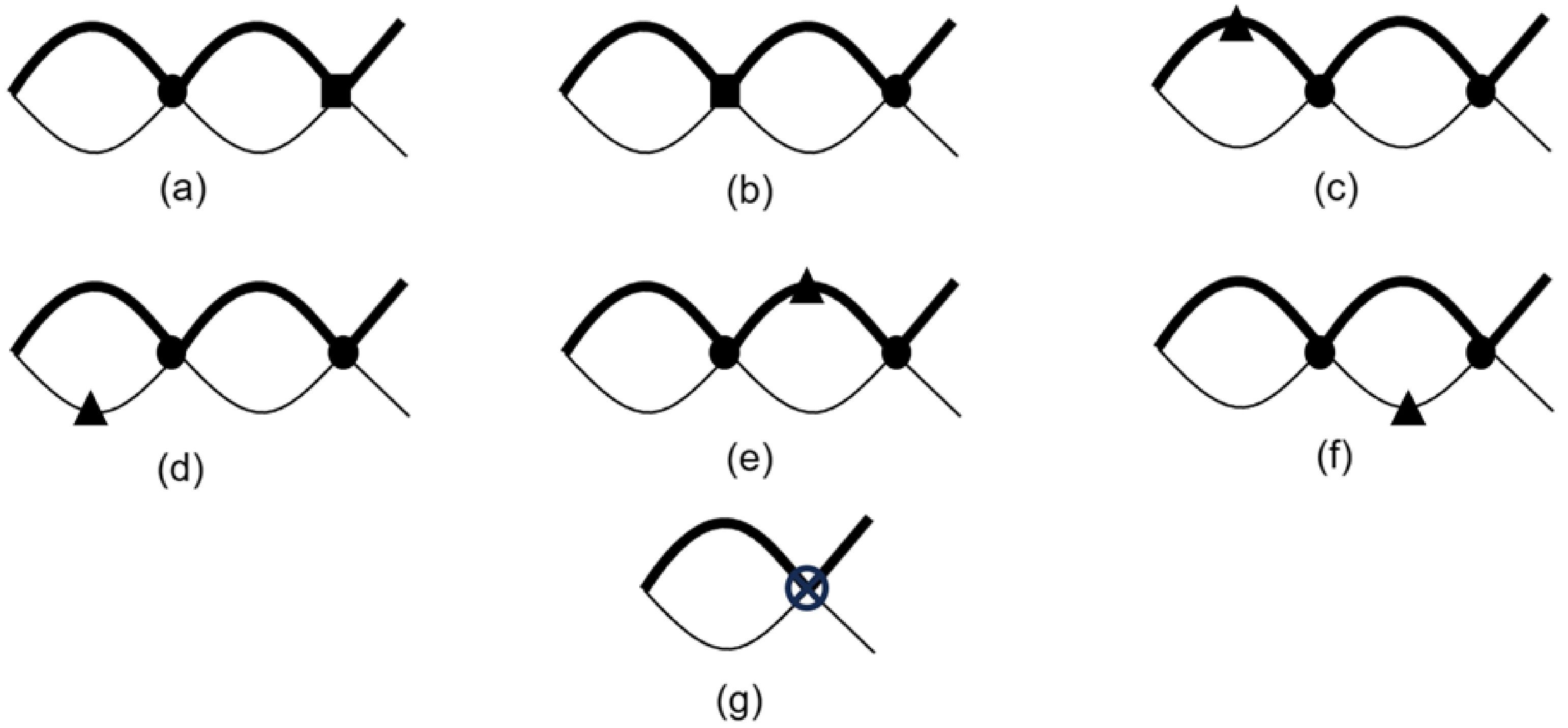
Figure 1. Potential-loop topologies that contribute to the two-loop current anomalous dimensions. Solid dots denote Coulomb potentials; solid squares denote the
$ V_r $ ,$ V_{2o} $ , and$ V_s $ potentials; solid triangles denote separate$ {\bf{p}}^4/(8m_b^3) $ or$ {\bf{p}}^4/(8m_c^3) $ kinetic insertions; and the crossed circle denotes the$ 1/|{\bf{k}}| $ potential. Diagrams (a) and (b) yield Eqs. (39) and (40), diagrams (c)–(f) yield Eq. (48), and diagram (g) yields Eq. (53).$ \begin{aligned}[b] {\cal{A}}_a=\;&\mu_S^{4\epsilon}\int_{{\bf{q}},{\bf{q}}'} \frac{{\cal{V}}_c^{[1]}} {D({\bf{q}})D({\bf{q}}')({\bf{q}}-{\bf{q}}')^2} \bigg[ \frac{{\cal{V}}_r^{[1]}({\bf{p}}^2+{\bf{q}}'^2)} {2m_bm_c({\bf{p}}-{\bf{q}}')^2} \\& +\frac{{\cal{V}}_s^{[1]}S(S+1)}{m_bm_c} -\frac{{\cal{V}}_{2o}^{[1]}(m_b-m_c)^2} {8m_b^2m_c^2} \bigg]. \end{aligned} $
(38) Expanding the large-momentum contribution relevant to the logarithmic pole yields
$\begin{aligned}[b] {\cal{A}}_a\big|_{\rm{UV}} =\;&-\frac{4x}{(1+x)^2}{\cal{V}}_c^{[1]} \bigg[ \frac{{\cal{V}}_r^{[1]}}{2} +S(S+1){\cal{V}}_s^{[1]}\\& -\frac{(1-x)^2}{8x}{\cal{V}}_{2o}^{[1]} \bigg] \frac{1}{64\pi^2\epsilon_{\rm{UV}}},\end{aligned} $
(39) $ {\cal{A}}_b\big|_{\rm{UV}} =-\frac{4x}{(1+x)^2}{\cal{V}}_c^{[1]} \frac{{\cal{V}}_r^{[1]}}{2} \frac{1}{64\pi^2\epsilon_{\rm{UV}}}. $
(40) The factor
$ 4x/(1+x)^2 $ arises from the two unequal-mass denominators in Eq. (28), before applying the reduced-mass simplification. Adding Eqs. (39) and (40) gives$ \begin{aligned}[b] \left.({\cal{A}}_a+{\cal{A}}_b)\right|_{\rm{UV}} =\;&-\frac{x}{16\pi^2(1+x)^2\epsilon_{\rm{UV}}}\, {\cal{V}}_c^{[1]}\\&\times \left[ {\cal{V}}_r^{[1]}+S(S+1){\cal{V}}_s^{[1]} -\frac{(1-x)^2}{8x}{\cal{V}}_{2o}^{[1]} \right], \\ \delta\widetilde Z_{S,{\rm{pot}}} =\;&\frac{x}{16\pi^2(1+x)^2\epsilon_{\rm{UV}}}\, {\cal{V}}_c^{[1]} \Bigg[ {\cal{V}}_r^{[1]}+S(S+1){\cal{V}}_s^{[1]} \\&-\frac{(1-x)^2}{8x}{\cal{V}}_{2o}^{[1]} \Bigg]. \end{aligned} $
(41) For each tree-level potential insertion,
$ {\cal{V}}_{i,B}=\mu_S^{2\epsilon}{\cal{V}}_i $ . Thus, with the bare potential coefficients held fixed,$ \frac{d}{d\ln\mu_S} \left({\cal{V}}_c^{[1]}{\cal{V}}_i^{[1]}\right) =-4\epsilon\, {\cal{V}}_c^{[1]}{\cal{V}}_i^{[1]} +{\cal{O}}(\alpha_s^3). $
(42) At this order,
$ \ln\widetilde Z_S=\delta\widetilde Z_S $ , and therefore$\begin{aligned}[b] \gamma_{{\rm{pot}}} =\;&-4\epsilon\,\delta\widetilde Z_{S,{\rm{pot}}} =-\frac{x}{4\pi^2(1+x)^2}\, {\cal{V}}_c^{[1]}\\&\times \left[ {\cal{V}}_r^{[1]}+S(S+1){\cal{V}}_s^{[1]} -\frac{(1-x)^2}{8x}{\cal{V}}_{2o}^{[1]} \right].\end{aligned} $
(43) At this point, we substitute the matching values into Eq. (34). Comparing the result with Eq. (20) yields
$ \gamma_{{\rm{pot}}}^{(2)} =-\frac{4x\pi^2 C_F^2}{(1+x)^2} \left[ 1-\frac{S(S+1)}{3}-\frac{(1-x)^2}{8x} \right]. $
(44) Diagrams (c)–(f) each contain one relativistic kinetic insertion. For example, the energy integral in diagram (e), which includes the double pole generated by the insertion on the antibottom line, yields
$ {\cal{A}}_e= \mu_S^{4\epsilon}\int_{{\bf{q}},{\bf{q}}'} \frac{({\cal{V}}_c^{[1]})^2}{8m_b^3} \frac{({\bf{q}}'^2)^2} {D({\bf{q}})[D({\bf{q}}')]^2 ({\bf{q}}-{\bf{q}}')^2({\bf{p}}-{\bf{q}}')^2}. $
(45) The corresponding insertion on the charm line is
$ {\cal{A}}_f= \mu_S^{4\epsilon}\int_{{\bf{q}},{\bf{q}}'} \frac{({\cal{V}}_c^{[1]})^2}{8m_c^3} \frac{({\bf{q}}'^2)^2} {D({\bf{q}})[D({\bf{q}}')]^2 ({\bf{q}}-{\bf{q}}')^2({\bf{p}}-{\bf{q}}')^2}, $
(46) which follows from the interchange
$ m_b\leftrightarrow m_c $ . Their logarithmic pole parts are obtained directly from the simultaneous ultraviolet limit. For the momentum routing in Eqs. (45) and (46),$ {\bf{q}}' $ denotes the momentum flowing through the propagator on which the kinetic operator is inserted, and thus through the double denominator$ [D({\bf{q}}')]^2 $ . Explicitly,$ \frac{({\bf{q}}'^2)^2} {D({\bf{q}})[D({\bf{q}}')]^2} \xrightarrow[|{\bf{q}}|,|{\bf{q}}'|\to\infty]{} -\frac{(2m_r)^3}{{\bf{q}}^2}. $
(47) The minus sign arises from the single unsquared heavy-pair denominator
$ D({\bf{q}}) $ . Including the insertion factors$ 1/(8m_b^3) $ and$ 1/(8m_c^3) $ yields$ \begin{aligned}[b]& {\cal{A}}_e\big|_{\rm{UV}} =-\frac{({\cal{V}}_c^{[1]})^2}{8m_b^3} \left(\frac{2m_bm_c}{m_b+m_c}\right)^3 \frac{1}{64\pi^2\epsilon_{\rm{UV}}}, \\& {\cal{A}}_f\big|_{\rm{UV}} =-\frac{({\cal{V}}_c^{[1]})^2}{8m_c^3} \left(\frac{2m_bm_c}{m_b+m_c}\right)^3 \frac{1}{64\pi^2\epsilon_{\rm{UV}}}, \end{aligned} $
(48) whereas
$ {\cal{A}}_c|_{\rm{UV}}={\cal{A}}_d|_{\rm{UV}}=0 $ . After symmetrization of the spatial integrals, the latter two topologies are logarithmically UV finite; their remaining power divergences vanish in dimensional regularization. Summing the two poles in Eq. (48)$ \left.({\cal{A}}_e+{\cal{A}}_f)\right|_{\rm{UV}} =-\frac{({\cal{V}}_c^{[1]})^2}{64\pi^2\epsilon_{\rm{UV}}} \frac{1-x+x^2}{(1+x)^2}. $
(49) Using the same two-potential argument as in Eq. (42),
$\begin{aligned}[b] \gamma_{\rm{kin}} =\;&-4\epsilon\left[ \frac{({\cal{V}}_c^{[1]})^2}{64\pi^2\epsilon_{\rm{UV}}} \frac{1-x+x^2}{(1+x)^2} \right] \\=\;&-\frac{({\cal{V}}_c^{[1]})^2}{16\pi^2} \frac{1-x+x^2}{(1+x)^2} =-\alpha_s^2C_F^2\frac{1-x+x^2}{(1+x)^2}.\end{aligned} $
(50) In the final equality, we have used the matching value of
$ {\cal{V}}_c^{[1]} $ . Comparison with Eq. (20) then yields$ \gamma_{\rm{kin}}^{(2)} =-\pi^2C_F^2\frac{1-x+x^2}{(1+x)^2}. $
(51) Finally, diagram (g) involves a single
$ 1/|{\bf{k}}| $ potential:$ {\cal{A}}_g= -\mu_S^{2\epsilon}\int_{{\bf{q}}} \frac{1}{D({\bf{q}})} \frac{\pi^2{\cal{V}}_k^{[1]}} {2m_r|{\bf{q}}-{\bf{p}}|}. $
(52) Using
$ D({\bf{q}})\to-{\bf{q}}^2/(2m_b)-{\bf{q}}^2/(2m_c) $ in the ultraviolet region, together with Eq. (30), gives$ {\cal{A}}_g\big|_{\rm{UV}} =\frac{{\cal{V}}_k^{[1]}}{4\epsilon_{\rm{UV}}}. $
(53) We initially treat
$ {\cal{V}}_k^{[1]} $ as an independent EFT Wilson coefficient. Because there is only one potential insertion,$ {\cal{V}}_{k,B}^{[1]}=\mu_S^{2\epsilon}{\cal{V}}_k^{[1]} $ and$ d{\cal{V}}_k^{[1]}/d\ln\mu_S=-2\epsilon{\cal{V}}_k^{[1]} $ with the bare coefficient held fixed. Equations (53) and (37) therefore give$ \delta\widetilde Z_{S,1/|{\bf{k}}|} =-\frac{{\cal{V}}_k^{[1]}}{4\epsilon_{\rm{UV}}}, \qquad \gamma_{1/|{\bf{k}}|} =-2\epsilon\,\delta\widetilde Z_{S,1/|{\bf{k}}|} =\frac{{\cal{V}}_k^{[1]}}{2}. $
(54) After performing this differentiation, we insert the unequal-mass matching coefficient. Substitution of Eq. (36) and comparison with Eq. (20) gives
$ \gamma_{1/|{\bf{k}}|}^{(2)} =\pi^2\left[ \frac{x}{(1+x)^2}C_F^2-\frac{C_AC_F}{2} \right]. $
(55) Summing these contributions gives a unified expression for the pseudoscalar and vector currents:
3 $ \gamma_S^{(2)}(x) =-\pi^2\left[ \frac{C_FC_A}{2} +\frac{x^2+6x+1-\frac{8x}{3}S(S+1)} {2(1+x)^2}C_F^2 \right]. $
(56) The spin dependence enters via
$ {\bf{S}}^2=S(S+1) $ , with$ S=0 $ for the pseudoscalar current and$ S=1 $ for the vector current. Equation (56) is invariant under interchange of the two heavy-quark masses,$ x\to1/x $ , as expected.For the two phenomenologically relevant channels, Eq. (56) gives
$ \gamma_{S=0}^{(2)}(x) = -\pi^2\left[ \frac{C_FC_A}{2} +\frac{1+6x+x^2}{2(1+x)^2}C_F^2 \right], $
(57) $ \gamma_{S=1}^{(2)}(x) = -\pi^2\left[ \frac{C_FC_A}{2} +\frac{3x^2+2x+3}{6(1+x)^2}C_F^2 \right], $
(58) corresponding to the
$ B_c $ and$ B_c^* $ currents, respectively.These results are consistent with the residual infrared poles obtained in full-QCD matching calculations. Equation (57) reproduces the two-loop anomalous dimension of the pseudoscalar current inferred from the
$ B_c $ leptonic decay amplitude [11, 14], whereas Eq. (58) reproduces the corresponding vector-current result [15, 16]. To our knowledge, Eqs. (57) and (58) provide the first simultaneous direct vNRQCD derivation of the two unequal-mass matching-scale current anomalous dimensions in a spin-unified form [31]. This qualified statement is consistent with the earlier equal-mass effective-theory calculations cited above.As a further check, we take the equal-mass limit
$ x\to1 $ . Equation (56) becomes$ \gamma_{S=0}^{(2)}(1) = -\pi^2C_F\left(C_F+\frac{C_A}{2}\right), $
(59) $ \gamma_{S=1}^{(2)}(1) = -\pi^2C_F\left(\frac{C_F}{3}+\frac{C_A}{2}\right), $
(60) This is in agreement with direct equal-mass effective-theory analyses and with the known matching results in the
$ d/d\ln\mu_\Lambda $ convention [11, 15, 22, 32].4 This smooth limit provides a stringent check of both the unequal-mass formula and the convention conversion.Finally, we summarize the two RG roles. The vNRQCD diagrams evaluated with the potential coefficients at their matching boundary
$ \nu=1 $ determine the$ {\cal{O}}(\alpha_s^2) $ anomalous dimension of the ordinary factorization-scale RGE in Eq. (20). This coefficient governs the$ \mu_\Lambda $ dependence of the current throughout the perturbative range and cancels the residual infrared poles in the full-QCD SDCs. Velocity evolution below$ \nu=1 $ follows the correlated derivative in Eq. (16). It generates unequal-mass mixed structures and the sum operators$ {\cal{O}}_{k1}^{(S)} $ and$ {\cal{O}}_{k2}^{(S)} $ of Ref. [26], together with running potentials arising from the soft-loop contractions discussed above. The present result provides the ordinary$ \mu_\Lambda $ evolution kernel and the matching-boundary input for a complete future VRG analysis. -
We now integrate the ordinary
$ \mu_\Lambda $ RGE in Eq. (24). The coefficient$ \gamma_S^{(2)}(x) $ is obtained from the minimal-subtraction ultraviolet pole and governs the fixed-order factorization-scale dependence of the current at perturbative values of$ \mu_\Lambda $ . The matching values of the potentials at$ \nu=1 $ determine this$ {\cal{O}}(\alpha_s^2) $ coefficient. The numerical curves below show the resulting factorization-scale evolution of the leading current. In contrast, complete velocity evolution follows the correlated trajectory$ (\mu_S,\mu_U)=(m_b\nu,m_b\nu^2) $ and incorporates the running potentials and induced operators described above.The HPQCD decay constant is a continuum-limit QCD observable extracted using a specific lattice-current normalization and extrapolation procedure [20], and it is independent of the
$ \overline{\rm{MS}} $ NRQCD factorization scale. Relating an absolute lattice matrix element to the vNRQCD LDME in Eq. (23) requires a scheme-matched SDC. We therefore use the dimensionless factorization-scale evolution ratio:$ U_H(\mu_\Lambda,\mu_{\rm{ref}}) \equiv \frac{\langle0|J_S(\mu_\Lambda)|H({\bf{P}})\rangle} {\langle0|J_S(\mu_{\rm{ref}})|H({\bf{P}})\rangle}. $
(61) This normalization eliminates dependence on the absolute normalization of the lattice current and isolates the running induced by the anomalous dimension at the stated perturbative accuracy. The residual dependence on the scheme and scale provides an estimate of the perturbative truncation uncertainty.
We use the standard potential-model scale masses
$ m_c=1.50\; {\rm{GeV}},\qquad m_b=4.80\; {\rm{GeV}}, $
(62) which are representative of heavy-quark phenomenology [7], and choose the reference point and the lower endpoint
$ \mu_{\rm{ref}}=\sqrt{m_bm_c}=2.683\; {\rm{GeV}}, \qquad \mu_{\rm{low}}=m_c=1.50\; {\rm{GeV}}. $
(63) The choice
$ \mu_{\rm{ref}}=\sqrt{m_bm_c} $ is distinguished by two structural properties of the unequal-mass problem: it is invariant under interchange of the heavy masses and exactly removes the explicit fixed-order factorization logarithm$ \ln[\mu_\Lambda^2/(m_bm_c)] $ in the SDC [16]. It is therefore the natural symmetric normalization point for the evolution factor in Eq. (61). The denominator of this ratio is a normalization convention that is independent of the hard matching scale. QCD-to-vNRQCD matching remains at$ \nu=1 $ , where$ \mu_S=\mu_U=m_b $ , while$ \sqrt{m_bm_c} $ serves as the reference point for the normalized LDME ratio. Thus,$ U_H(\mu_{\rm{ref}},\mu_{\rm{ref}})=1 $ follows directly from its definition. A normalization at$ m_b $ is related by the composition law$ U_H(\mu_\Lambda,m_b) =U_H(\mu_\Lambda,\mu_{\rm{ref}})\, U_H(\mu_{\rm{ref}},m_b), $
(64) and yields the same physical product of the SDC and LDME to the stated accuracy. The horizontal axis in the plots denotes the factorization scale
$ \mu_\Lambda $ ; the subtraction velocity ν labels the corresponding correlated soft–ultrasoft trajectory. We take$ \mu_{\rm{low}}=m_c $ as the lower endpoint; the interval remains perturbative in both fixed-flavor coupling conventions considered below.At one-loop accuracy, we use
$ \frac{1}{\alpha_s^{(n_f)}(\mu)} = \frac{1}{\alpha_s^{(n_f)}(\mu_0)} +\frac{\beta_0^{(n_f)}}{2\pi}\ln\frac{\mu}{\mu_0}, \qquad \beta_0^{(n_f)}=11-\frac{2n_f}{3}. $
(65) To facilitate combination with SDCs expressed in either a three- or four-flavor coupling convention, we carry out the illustrative evolution for both
$ n_f=3 $ and$ n_f=4 $ , while keeping the chosen value fixed throughout the interval$ \mu_{\rm{low}}\leq\mu_\Lambda\leq\mu_{\rm{ref}} $ .Combining Eq. (24) with the one-loop running of the coupling yields
$ U_H(\mu_\Lambda,\mu_{\rm{ref}}) = \exp\left[ +\frac{2\gamma_S^{(2)}(x)}{\beta_0^{(n_f)}\pi} \left(\alpha_s^{(n_f)}(\mu_\Lambda) -\alpha_s^{(n_f)}(\mu_{\rm{ref}})\right) \right]. $
(66) Here,
$n_f$ is the number of active flavors in the fixed-flavor coupling$\alpha_s^{(n_f)}$ . Equation (66) resums the conventional factorization-scale logarithms generated by the$ {\cal{O}}(\alpha_s^2) $ current anomalous dimension with one-loop coupling running. Velocity logarithms are governed separately by the VRG in Eq. (16). The fixed-order expansion begins at$ {\cal{O}}[\alpha_s^2\ln(\mu_\Lambda/\mu_{\rm{ref}})] $ . Here, S denotes the spin of$ H=B_c $ or$ B_c^* $ . For$ x=m_c/m_b=0.3125 $ , Eqs. (57) and (58) give$ \gamma_{S=0}^{(2)}=-34.8781, \qquad \gamma_{S=1}^{(2)}=-26.3902. $
(67) The corresponding endpoint ratios are
$ U_{B_c}(\mu_{\rm{low}},\mu_{\rm{ref}}) = \left\{ {\begin{array}{*{20}{l}} {0.8629,}&{{n_f} = 3,}\\ {0.8609,}&{{n_f} = 4,} \end{array}} \right. $
(68a) $ U_{B_c^*}(\mu_{\rm{low}},\mu_{\rm{ref}}) = \left\{ {\begin{array}{*{20}{l}} {0.8944,}&{{n_f} = 3,}\\ {0.8929,}&{{n_f} = 4.} \end{array}} \right. $
(68b) Thus, under this leading factorization-scale evolution, lowering the scale from
$ 2.683 $ to$ 1.50\; {\rm{GeV}} $ decreases the pseudoscalar LDME by approximately$ 13.7$ % ($ 13.9$ %) and the vector LDME by approximately$ 10.6$ % ($ 10.7$ %) for$ n_f=3 $ ($ n_f=4 $ ). The larger effect in the pseudoscalar channel reflects the greater magnitude of$ \gamma_{S=0}^{(2)} $ . These percentages quantify the current anomalous-dimension contribution; complete velocity running also incorporates the potential and mixing effects described above. -
The ratios shown in Fig. 2 describe the factorization-scale dependence of the leading vNRQCD current. Predictions for the physical decay constants also require the SDCs and power-suppressed matrix elements. For the pseudoscalar channel, the Standard Model leptonic width is given by
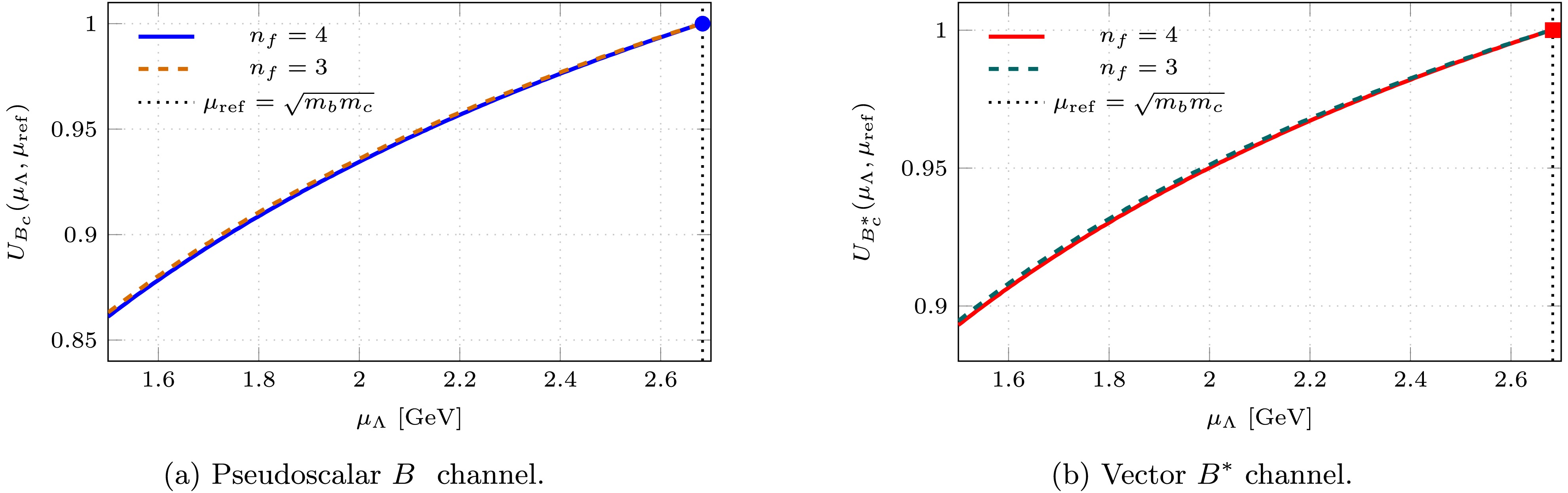
Figure 2. (color online) Factorization-scale running ratios for the leading
$ B_c $ and$ B_c^* $ LDMEs, generated by Eqs. (57) and (58). The parameters are set to$ m_c=1.50\; {\rm{GeV}} $ ,$ m_b=4.80\; {\rm{GeV}} $ , and$ \mu_{\rm{ref}}=2.683\; {\rm{GeV}} $ . The solid and dashed curves correspond to the$ n_f=4 $ and$ n_f=3 $ coupling conventions, respectively; the dotted vertical line indicates$ \mu_{\rm{ref}} $ .$ \begin{aligned}[b]&\Gamma(B_c^+\to\ell^+\nu_\ell) \\=\;&\frac{G_F^2|V_{cb}|^2}{8\pi}\, f_{B_c}^2M_{B_c}m_\ell^2 \left(1-\frac{m_\ell^2}{M_{B_c}^2}\right)^2 \left(1+\delta_{\rm EW+QED}\right). \end{aligned}$
(69) Therefore, a future measurement of the branching fraction would determine
$ f_{B_c}|V_{cb}| $ . Neglecting smaller parametric terms in this discussion, the linearized fractional variation satisfies$ \frac{\delta|V_{cb}|}{|V_{cb}|} =\frac12\frac{\delta{\cal{B}}}{{\cal{B}}} -\frac12\frac{\delta\tau_{B_c}}{\tau_{B_c}} -\frac{\delta f_{B_c}}{f_{B_c}}+\cdots . $
(70) The decay-constant uncertainty therefore propagates linearly into an extraction of
$ |V_{cb}| $ , rather than being reduced by the factor$ 1/2 $ that applies to the decay rate.Such a precision extraction requires power-suppressed operators in addition to the leading-current contribution. Up to relative order
$ v^2 $ , the pseudoscalar factorization formula may be written in the conventions of Ref. [33] as$\begin{aligned}[b] f_{B_c} =\;&\sqrt{\frac{2}{M_{B_c}}} \Big[P_0(\mu_\Lambda)\langle{\cal{O}}_0(\mu_\Lambda)\rangle \\&+P_1(\mu_\Lambda)\langle{\cal{O}}_1(\mu_\Lambda)\rangle +{\cal{O}}(v^4)\Big],\end{aligned} $
(71) $ {\cal{O}}_0 =\chi_b^\dagger\psi_c, $
(72) $ {\cal{O}}_1 =\chi_b^\dagger \left(-\frac{i}{2}\overleftrightarrow{\boldsymbol\nabla}\right)^2\psi_c . $
(73) Here,
$ P_0 $ denotes the temporal–axial coefficient associated with the spin-singlet current. The ordinary-derivative operator is defined in the Coulomb-gauge basis of Ref. [33], and$ \langle{{\boldsymbol{p}}}_{\rm{rel}}^2\rangle \equiv\langle{\cal{O}}_1\rangle/\langle{\cal{O}}_0\rangle $ . At tree level,$ \frac{P_1^{(0)}}{P_0^{(0)}} =-\frac{(m_b+m_c)^2}{8m_b^2m_c^2}. $
(74) For the masses
$ m_b=4.6\; {\rm{GeV}} $ and$ m_c=1.5\; {\rm{GeV}} $ used in Ref. [33], this coefficient is$ -0.09769\; {\rm{GeV}}^{-2} $ . The reference value$ \langle{{\boldsymbol{p}}}_{\rm{rel}}^2\rangle=0.124\; {\rm{GeV}}^2 $ adopted there is the midpoint of the renormalized$ \overline{\rm{MS}} $ $ J/\psi $ and$ \Upsilon(1S) $ benchmarks,$ 0.441 $ and$ -0.193\; {\rm{GeV}}^2 $ , rather than a direct$ B_c $ determination. These inputs yield a central tree-level derivative-current correction of$ -1.21$ %; evaluating the two endpoints gives$ -4.31$ % and$ +1.89$ %, respectively. These endpoint values are scheme-dependent benchmarks that illustrate the possible range of the correction. If this term were the dominant omitted correction, its fractional shift in$ f_{B_c} $ would induce an equal-magnitude shift of opposite sign in the extracted$ |V_{cb}| $ .A complete error estimate requires the relative-
$ v^2 $ coefficients and renormalized matrix elements to be specified in a common scheme, including$ {\cal{O}}(\alpha_s v^2) $ matching, operator mixing, and an estimate of the$ v^4 $ remainder. A lattice NRQCD calculation should determine both$ \langle{\cal{O}}_0\rangle $ and$ \langle{\cal{O}}_1\rangle $ with the corresponding continuum conversion and control the lower-dimensional mixing of$ {\cal{O}}_1 $ . Fully relativistic lattice calculations avoid an explicit velocity truncation; for example, HPQCD obtained$ f_{B_c}=0.427(6)(2)\; {\rm{GeV}} $ [20], corresponding to a total uncertainty of about$ 1.5$ % and thus the same fractional decay-constant contribution to a prospective$ |V_{cb}| $ extraction. This physical continuum-QCD decay constant is conceptually distinct from the scale-dependent leading-current matrix element shown in Fig. 2.Within vNRQCD, these power corrections arise from an enlarged basis of relative-
$ v^2 $ currents whose hard coefficients, renormalized matrix elements, and operator mixing must be treated in a single scheme. Their standard factorization-scale dependence must cancel that of the corresponding SDCs, whereas resumming velocity logarithms also requires the correlated soft and ultrasoft VRG evolution. A precision$ |V_{cb}| $ analysis therefore requires the leading result obtained here to be embedded in this extended vNRQCD factorization framework. -
We have directly calculated the two-loop anomalous dimensions of the leading flavor-changing NRQCD currents relevant to the leptonic decays of the
$ B_c $ and$ B_c^* $ mesons. Using the vNRQCD potential coefficients at their matching boundary$ \nu=1 $ , we obtained the$ {\cal{O}}(\alpha_s^2) $ anomalous dimension of the standard$ \mu_\Lambda $ RGE. The result is the unified expression in Eq. (56) for the pseudoscalar and vector channels, which are distinguished by the spin factor$ S(S+1) $ .Our results agree with the anomalous dimensions extracted from residual infrared poles in full-QCD matching calculations [11, 15, 16], and they reduce smoothly to the known equal-mass effective-theory results [22, 32]. These agreements provide a nontrivial check of NRQCD factorization for flavor-changing currents at two-loop order and confirm that vNRQCD provides a self-contained description of current renormalization at the matching point. The methodological advance of this work is a direct unequal-mass derivation that treats the pseudoscalar and vector channels simultaneously and explicitly demonstrates how the mode separation of vNRQCD controls the calculation.
The
$ 10$ % –$ 14$ % factorization-scale evolution shown in Fig. 2 indicates that this current contribution can be numerically important. Complete velocity evolution supplements this contribution with the running potentials and induced operators. Our result provides the unequal-mass, spin-resolved current contribution needed for a future combination of the complete VRG evolution, relativistic currents, and consistently matched lattice matrix elements. This combination provides the appropriate theoretical input for a precision extraction of$ |V_{cb}| $ .The next step within the same vNRQCD framework is to include the full unequal-mass velocity running of the potentials, the ultrasoft-induced operators and their pull-up counterterms, the line-diagonal wavefunction completion, and the genuine soft-loop contractions of subleading soft operators. The current basis should then be enlarged to relative order
$ v^2 $ and renormalized with the same mode separation, including the$ {\cal{O}}(\alpha_s^2v^2) $ contributions to the flavor-changing currents. This would place the velocity logarithms and the relativistic corrections entering a future$ |V_{cb}| $ analysis within a single internally consistent effective-theory framework.
Direct renormalization of flavor-changing currents in vNRQCD for ${{\boldsymbol B}_{\boldsymbol c}^{(*)}}$ decays
- Received Date: 2026-08-17
- Available Online: 2027-02-01
Abstract: We present a direct vNRQCD calculation of the two-loop anomalous dimensions of the leading flavor-changing nonrelativistic currents that govern the leptonic decays of the $ B_c $ and $ B_c^* $ mesons. Using the potential matching coefficients at the boundary $ \nu=1 $, we determine the ultraviolet counterterms for the currents directly within the effective theory. These counterterms provide the $ {\cal{O}}(\alpha_s^2) $ ordinary factorization-scale RGE required to cancel the residual infrared poles in the full-QCD short-distance coefficients. The pseudoscalar and vector channels are obtained from a single spin-unified formula, with the spin dependence entering through $ S(S+1) $. We also clarify the distinct role of the velocity RGE: the ultrasoft-induced mixing coefficients vanish at $ \nu=1 $ and become essential for the full velocity running below the matching boundary. The results agree with known matching calculations and reduce smoothly to the equal-mass quarkonium limits.



 DownLoad: