Empirical predictions of α-decay and spontaneous fission half-lives in the decay chains of elements 119 and 120

Alpha decay and spontaneous fission (SF) are the principal decay modes of heavy and superheavy nuclei (SHN) [1−7]. The unambiguous identification of new isotopes is greatly facilitated by the observation of their $ \alpha $-decay chains terminating in SF. Experimental and theoretical investigations of these nuclei constitute a major frontier in modern nuclear physics [8−21]. Consequently, a comprehensive understanding of the competition between $ \alpha $ decay and SF is indispensable for guiding experimental exploration and accurately mapping the extent and boundaries of the island of stability [1−3, 22−30].

Although various microscopic approaches have been developed to describe $ \alpha $ decay [31−35] and SF [36−42], their application to heavy and superheavy systems remains computationally demanding and sensitive to uncertainties in shell structure and fission barrier heights. These challenges have sustained strong interest in developing fast semi-empirical methods for systematic half-life predictions [43−55].

For $ \alpha $ decay, the Viola–Seaborg relation [45] remains a widely used semi-empirical tool. It is commonly expressed as

where Z is the proton number and $ Q_\alpha $ is the $ \alpha $-decay energy. In this work, we adopt the Parkhomenko–Sobiczewski parameterization [56], which, as demonstrated in Ref. [57], provides high accuracy for SHN when benchmarked against experimental $ T_{1/2}^{\alpha} $ data. The corresponding coefficients are $ a = 1.3892 $, $ b = 13.862 $, $ c = -0.1086 $, and $ d = -41.458 $, while $ h_{\alpha} = 0 $, 0.437, 0.641, and 1.024 for even-even, odd-even, even-odd, and odd-odd nuclei, respectively.

For SF half-lives, we have previously found that, at fixed $ N-Z $, $ \log_{10} T_{1/2}^{\rm{SF}} $ depends nearly linearly on $ Q_\alpha $ [58, 59]. This observation enabled us to derive an empirical formula that relates SF half-lives directly to the $ \alpha $-decay energy $ Q_\alpha $ and the neutron excess $ N-Z $:

where $ h_{\rm{SF}} = 0 $, h, and $ 1.575h $ for even-even, odd-A, and odd-odd nuclei, respectively. The coefficients are divided into two sets according to Z: for $ 90 \le Z \le 102 $, $ c_0 = -244.845 $, $ c_1 = 12.2843 $, $ c_2 = -0.12658 $, $ c_Q = -6.1023 $, and $ h = 4.309 $; for $ Z \ge 103 $, $ c_0 = -0.414 $, $ c_1 = 0.1379 $, $ c_2 = 0 $, $ c_Q = -0.9097 $, and $ h = 2.327 $. Because Eq. (2) uses only $ Q_\alpha $, which is typically determined more reliably than absolute masses or shell-correction energies [60], it avoids the model-dependent uncertainties inherent in microscopic fission calculations.

Most heavy and superheavy nuclei are deformed, and deformation can affect both $ \alpha $-decay and SF half-lives. Explicitly incorporating quadrupole and hexadecapole deformation parameters into the generalized liquid drop model has been shown to improve agreement with experimental data, particularly in the superheavy region [61]. Because the ground-state masses of the parent and daughter nuclei depend on their shapes, deformation is partially embedded in the $ \alpha $-particle separation energy $ Q_\alpha $. In the present work, therefore, deformation is treated implicitly through $ Q_\alpha $.

The aim of the present work is to investigate the competition between $ \alpha $ decay and SF along the $ \alpha $-decay chains of $ Z=119 $ and $ Z=120 $ isotopes, whose properties are currently the subject of intensive experimental and theoretical studies. For this purpose, we employ Eq. (1) and Eq. (2) to estimate the corresponding half-lives for nuclei in the $ \alpha $-decay chains of $ Z=119 $ isotopes with A = 293–298 and $ Z=120 $ isotopes with A = 295–300, extending down to Lr and Rf isotopes. The corresponding neutron-excess values, $ N-Z = 55 $ to 60, place these nuclei near the predicted island of stability, making their decay characteristics particularly relevant for guiding future experimental efforts at the limits of the nuclear chart. The novelty of the present work lies in its systematic mapping of this competition and its identification of robust experimental decay chains.

To obtain an overall picture of the competition between $ \alpha $ decay and SF in the region of interest, we first calculate the partial half-lives using the formulas described above. The $ \alpha $-decay half-life $ T_{1/2}^\alpha $ is obtained from Eq. (1), whereas the SF half-life $ T_{1/2}^{\rm{SF}} $ is calculated using Eq. (2). Both formulas require the $ \alpha $-decay energy $ Q_\alpha $ as input.

The calculations use experimental $ Q_\alpha $ values from Ref. [62] whenever available; otherwise, the values are taken from the macroscopic–microscopic model of Ref. [63]. This model combines the Yukawa-plus-exponential macroscopic energy [64] with microscopic shell and pairing corrections obtained via the Strutinsky method from the single-particle levels of a deformed Woods–Saxon potential. It is widely used in this mass region and provides calculated $ Q_\alpha $ values for all nuclei of interest. To quantify its accuracy, we define the deviation for $ Q_\alpha $ as $ \delta^{Q_\alpha} = Q_\alpha^{{\rm{calc}}.} - Q_\alpha^{{\rm{exp}}.} $. Its performance against the experimental $ Q_\alpha $ data from Ref. [62] is characterized by a mean deviation (indicating overestimation) of $ \langle \delta^{Q_\alpha} \rangle = 136 $ keV, a mean absolute deviation of $ \langle \left| \delta^{Q_\alpha} \right| \rangle = 260 $ keV, and a root-mean-square deviation of $ \delta_{\rm{rms}}^{Q_\alpha} = 315 $ keV, evaluated for 92 nuclei with $ Z \ge 103 $.

To assess the quality of the description, the calculated half-lives for both decay modes are compared with experimental data. For $ \alpha $-decay half-lives, the primary source is Ref. [7], supplemented by the most recent experimental data for ²⁷²Hs, ²⁷⁵Ds [13], ²⁷⁶Ds [12], and ²⁵⁷Sg [15]. The ground-state half-lives of ²⁶¹Rf, ²⁶⁵Sg, ²⁷¹Hs, and ²⁷³Ds are updated according to the one-quasiparticle level schemes proposed in Ref. [13]. Additional data for ²⁵¹Lr [65], ²⁵³Rf [30], ²⁵⁷Db [66], ²⁶⁸Db [9, 11], ²⁷²Bh, ^282–285Nh and ²⁸⁶Mc [11], ²⁵⁸Sg [67], ²⁶²Sg [68], ²⁶⁴Sg [25], ²⁶⁹Sg, ²⁸¹Cn, ²⁸⁹Lv [69], ²⁸⁸Lv [70], ²⁷¹Sg, ²⁷⁵Hs, ²⁸³Cn, ²⁸⁶Fl [10], ²⁶⁵Bh [71], ²⁶⁴Hs [29], ²⁶⁷Hs [24], ²⁷³Hs [72], ²⁸²Mt, ²⁸⁶Rg, ²⁸⁴Fl [23], and ²⁸⁴Cn [20] are also included, with half-lives and branching ratios (or their limits) taken from the original publications or updated as necessary.

For SF half-lives, experimental values are taken primarily from Refs. [7, 29], together with the recently reported half-lives of ²⁵²Rf [14], ²⁶³Rf [13], ²⁶⁴Lr [9, 11], ²⁵⁷Db [66], ²⁶⁶Db [11], ²⁵⁷Sg [15], ²⁶⁸Sg, and ²⁷⁶Ds [12]. In addition, the data for ²⁵⁵Lr [73], ^267,268Db, ^279,281Rg, ²⁸⁵Nh [11], ²⁷⁷Mt [74], ²⁵⁹Sg [75], ²⁶⁹Sg, ²⁸¹Cn [69], ²⁶⁰Bh [76], ²⁶⁵Hs [77], ²⁷⁰Hs [78], ²⁷⁵Hs [10], and ²⁸⁴Fl [23] are updated or supplemented, including branching ratios and half-life limits where applicable.

To validate the use of theoretical $ Q_\alpha $ values from Ref. [63] in the present calculations, we compare the resulting half-lives with experimental data. Nuclei for which only limits are available were excluded from the statistical analysis. For each decay mode m ($ m=\alpha $ or SF), we define the deviation as $ \delta^{T_{1/2}^{m}} = \log_{10} ( T_{1/2}^{m,\,{{\rm{calc}}.}} / T_{1/2}^{m,\,{{\rm{exp}}.}} ) $. For 120 nuclei with $ Z \ge 103 $ and known experimental $ \alpha $-decay half-lives, the use of theoretical $ Q_\alpha $ values in Eq. (1) yields a mean absolute deviation $ \langle | \delta^{T_{1/2}^{\alpha}} | \rangle = 0.80 $ orders of magnitude and a root-mean-square deviation $ \delta_{{\rm{rms}}}^{T_{1/2}^{\alpha}} = 1.10 $. For 59 nuclei with $ Z \ge 103 $ and known experimental SF half-lives, the same $ Q_\alpha $ input in Eq. (2) gives $ \langle | \delta^{T_{1/2}^{{\rm{SF}}}} | \rangle = 0.97 $ orders of magnitude and $ \delta_{{\rm{rms}}}^{T_{1/2}^{{\rm{SF}}}} = 1.40 $. These deviations are within the typical accuracy of empirical systematics and confirm that the formulas reproduce the overall magnitudes of the half-lives. We therefore use theoretical $ Q_\alpha $ values for all nuclei for which experimental values are unavailable.

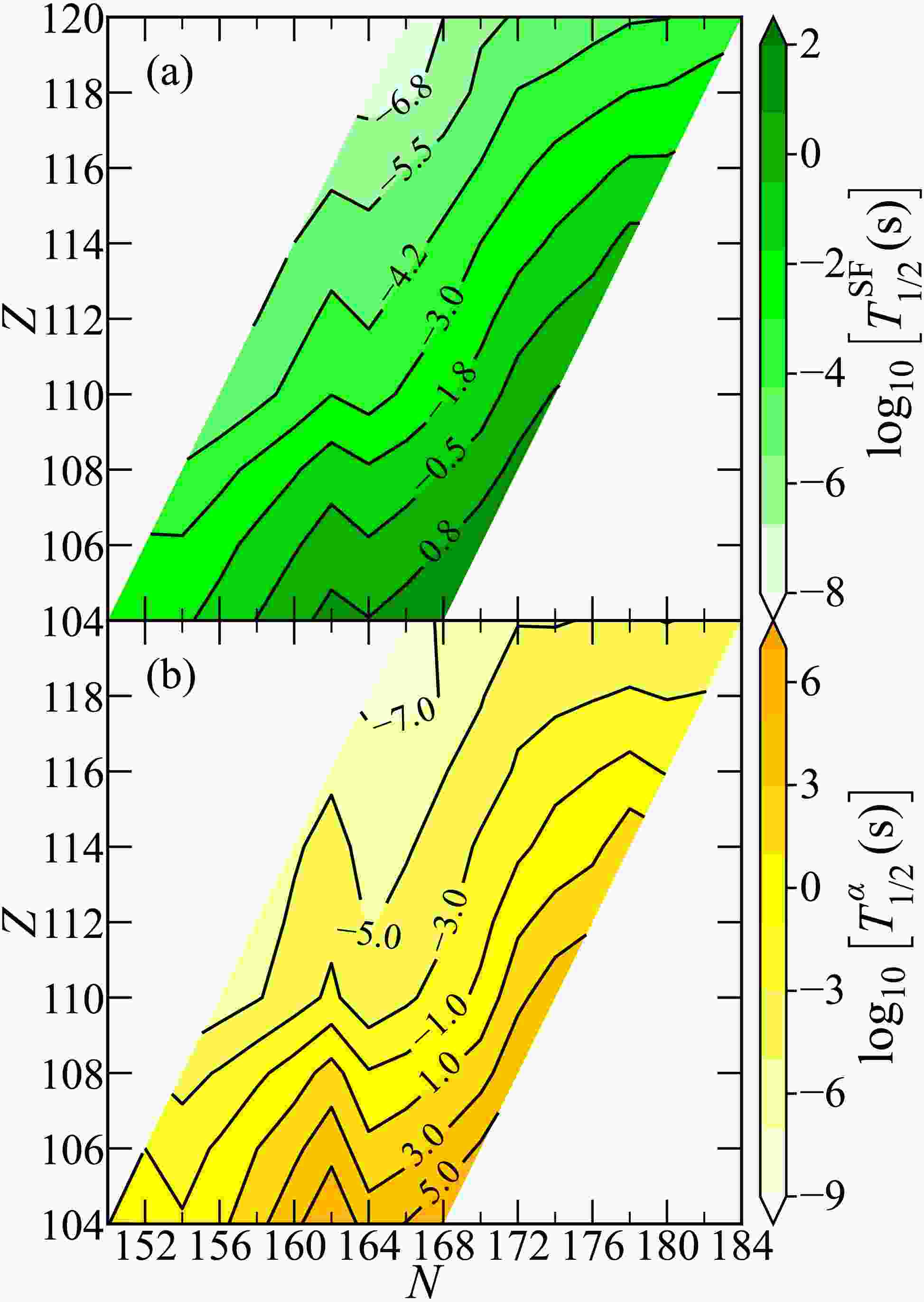
Figure 1 presents contour maps of the logarithms of the calculated half-lives for SF and $ \alpha $ decay of even-even nuclei in the region $ 104 \le Z \le 120 $ and $ 46 \le N-Z \le 64 $. The calculations use $ Q_\alpha $ values obtained from Ref. [63]. The half-lives exhibit smooth trends, decreasing gradually with decreasing neutron excess and increasing proton number. In contrast to shell-correction energies, which typically exhibit pronounced structures around magic numbers [79−81], the half-lives vary more smoothly across the considered region. Although the formulas used for both decay modes do not explicitly include shell corrections, shell-structure information enters through the $ Q_\alpha $ values and is reflected in the observed half-life variations. An increase in both SF and $ \alpha $-decay half-lives is observed near the deformed shell closure at $ N=162 $. Within the present semi-empirical description, the enhancement of the half-lives associated with this shell closure is less pronounced for SF than for $ \alpha $ decay.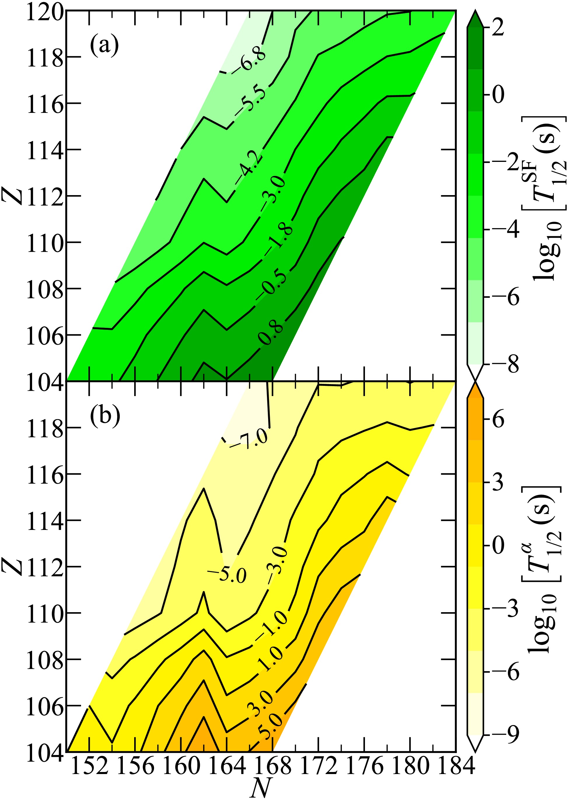

Figure 1.  (color online) Color contour maps show the logarithms of SF (a) and $ \alpha $-decay (b) half-lives, expressed in seconds, for even-even nuclei with proton numbers $ 104 \le Z \le 120 $ and neutron excess $ 46 \le N-Z \le 64 $. The half-lives were calculated using Eq. (1) for $ \alpha $ decay and Eq. (2) for SF, with $ Q_\alpha $ values from Ref. [63].

Figures 2 and 3 present the calculated partial half-lives for $ \alpha $ decay and SF along the $ \alpha $-decay chains of $ Z=119 $ and $ Z=120 $ isotopes, respectively, in comparison with experimental data. Experimental $ Q_\alpha $ values from Ref. [62] are used where available; otherwise, theoretical $ Q_\alpha $ values from Ref. [63] are employed.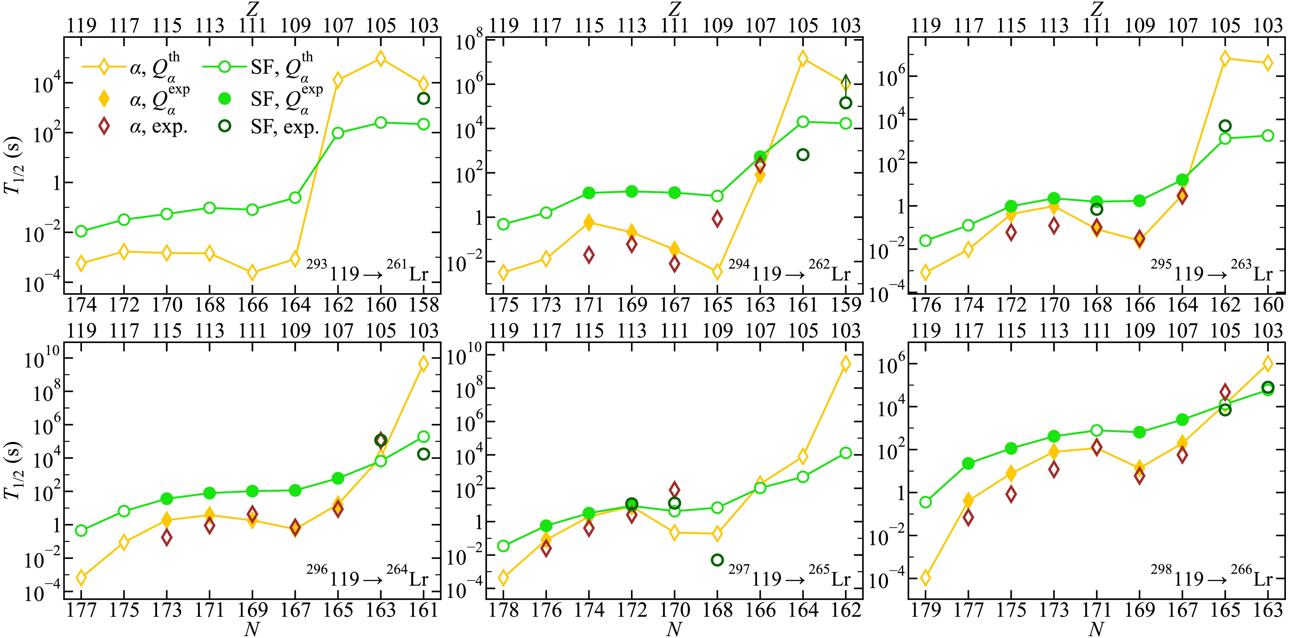

Figure 2.  (color online) Comparison of the calculated $ \alpha $-decay (yellow diamonds connected by lines) and SF (green circles connected by lines) half-lives for $ \alpha $-decay chains originating from isotopes of element 119 with mass numbers A = 293–298. The $ \alpha $-decay and SF half-lives are calculated using Eq. (1) and Eq. (2), respectively. Solid symbols denote calculations based on experimental $ Q_\alpha $ values from Ref. [62], whereas open symbols denote calculations based on theoretical $ Q_\alpha $ values from Ref. [63]. Experimental $ \alpha $-decay (open brown diamonds) and SF (open darkgreen circles) half-lives are taken from Refs. [7, 29]. Downward (upward) arrows indicate upper (lower) limits on the half-life for the corresponding decay mode.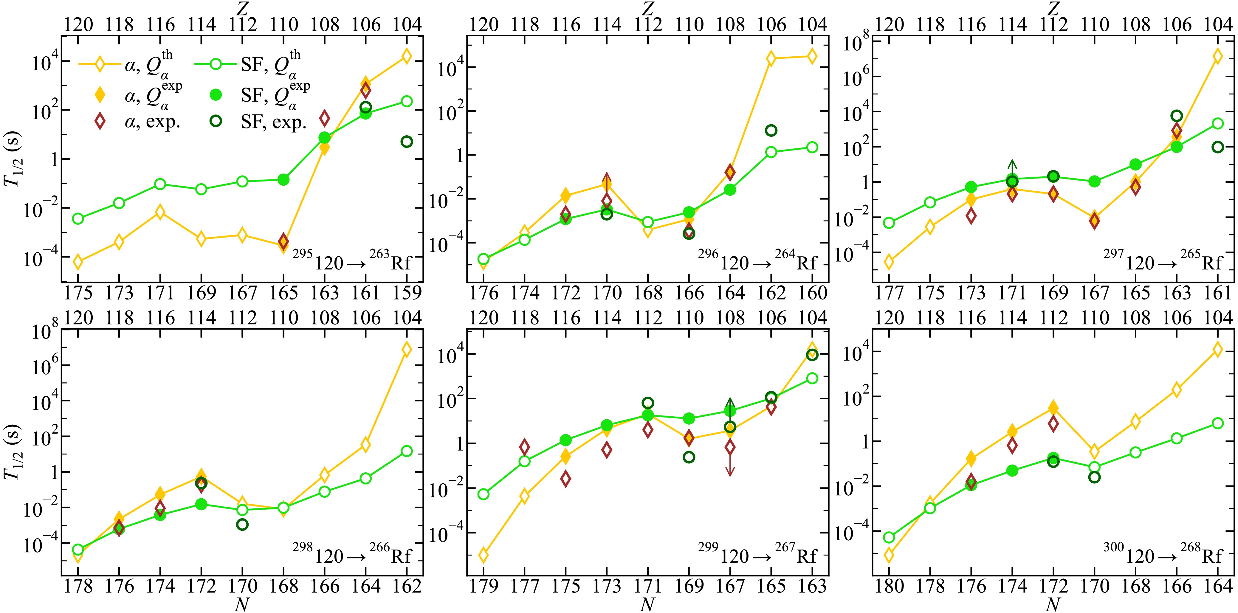

Figure 3.  (color online) Same as in Fig. 2, but for the $ \alpha $-decay chains of $ Z=120 $ isotopes with mass numbers A = 295–300.

A global trend observed in both figures is the decrease in the partial half-lives for both decay modes as one moves further into the superheavy region. The extent to which one decay mode dominates over the other can be assessed from the vertical separation between the two corresponding curves: the larger the separation, the higher the probability of decay through the mode with the shorter half-life.

For chains starting from ^293,294,296119 and ²⁹⁵120, $ \alpha $ decay clearly dominates over SF by about two orders of magnitude at the initial members of the chains. However, this behavior changes abruptly at neutron number $ N=162 $, where the $ \alpha $-decay half-lives increase sharply, whereas the SF half-lives exhibit a much less pronounced increase. Consequently, SF becomes the dominant decay mode for $ N<162 $. In contrast, for chains starting from ^295,297,298119 and ^297,299120, the two decay modes already exhibit strong competition from the initial steps of the chains, with SF clearly dominating for $ N<162 $. For chains initiated by ^296,298,300120, SF dominates almost immediately. A particularly prominent feature is observed at $ N=172 $, where the $ \alpha $-decay half-lives increase more substantially than the SF half-lives, leading to pronounced SF dominance.

Comparing the two elements, the half-lives of $ Z=119 $ isotopes are systematically longer than those of $ Z=120 $ isotopes. Odd-even effects are also evident: for even-Z-odd-N nuclei, the SF half-lives are noticeably longer than those of even-even nuclei, whereas the $ \alpha $-decay half-lives show much weaker sensitivity to these effects.

To further assess the predictive power of the approach, we compare the calculated dominant decay modes with experimental data for 64 nuclei with $ 103 \le Z \le 118 $ and $ 261 \le A \le 295 $. This set comprises the nuclei for which at least one partial half-life of the two considered decay modes is experimentally known with sufficient accuracy for a quantitative comparison. The full comparison of the calculated and experimental half-lives and branching ratios is given in Table 1 of Appendix A, which also includes two additional nuclei for which only limits on the branching ratios are available. The predicted dominant decay mode agrees with experiment in 53 cases. The remaining 11 discrepancies are discussed below and grouped according to the predicted dominant mode.

For ²⁷⁷Mt and ^279,281Rg, $ \alpha $ decay is predicted to dominate. For ²⁷⁷Mt, only SF has been observed, whereas for ²⁷⁹Rg and ²⁸¹Rg, the available experimental data on both modes indicate competition between $ \alpha $ decay and SF. Microscopic calculations of $ T_{1/2}^{{\rm{SF}}} $ are not available for these three nuclei. For ²⁸¹Rg, the WS4 model [82, 83] gives $ Q_\alpha = 9.76 $ MeV, which is 0.60 MeV lower than the value used here, and the corresponding $ T_{1/2}^{\alpha,\,{{\rm{calc}}.}} = 8.4 $ s is only about one order of magnitude smaller than the experimental value $ T_{1/2}^{\alpha,\,{{\rm{exp}}.}} = 79 $ s. For ²⁷⁷Mt, all considered models [63, 81, 83] give $ T_{1/2}^{{\rm{SF}},\,{{\rm{calc}}.}} \sim 10 $ s, which is three to four orders of magnitude larger than $ T_{1/2}^{{\rm{SF}},\,{{\rm{exp}}.}} = 5.0 $ μs. For ²⁷⁹Rg, the values calculated with $ Q_\alpha^{{\rm{exp}}} $ favour $ \alpha $ decay but differ only by a factor of 19, which is still consistent with the experimentally observed competition.

For ^286,288Fl and ^288,290,292Lv, SF is predicted to dominate. For ²⁸⁶Fl, the available experimental data on both modes indicate competition between $ \alpha $ decay and SF, whereas for ²⁸⁸Fl and the Lv isotopes, only $ \alpha $ decay has been detected so far. The microscopic models show considerable disagreement for these nuclei when compared with the $ T_{1/2}^{\alpha} $ values calculated from $ Q_\alpha^{{\rm{exp}}} $ using Eq. (1). For ²⁸⁸Fl, Ref. [84] predicts SF dominance, whereas Refs. [36, 38] favour $ \alpha $ decay. For ²⁸⁶Fl and ²⁸⁸Lv, Ref. [39] predicts SF dominance, Refs. [36−38] favour $ \alpha $ decay, and Ref. [84] predicts competition. For ²⁹²Lv and ²⁹⁰Lv, Refs. [39, 84] predict competition, whereas Refs. [37, 38] favour $ \alpha $ decay. In particular, for ²⁹⁰Lv, Refs. [39] and [84] give $ T_{1/2}^{{\rm{SF}}} = 13 $ ms and 10 ms, respectively, which are comparable to the $ T_{1/2}^{\alpha} = 52 $ ms calculated from $ Q_\alpha^{{\rm{exp}}} $ using Eq. (1) and thus lead to the same competition between the two modes. In contrast, Refs. [37] and [38] give $ T_{1/2}^{{\rm{SF}}} = 12 $ min and 3 y, respectively, and therefore favour $ \alpha $ decay.

For ²⁷²Hs, ²⁸³Cn, and ²⁹⁴Og, competition between $ \alpha $ decay and SF is predicted. For ²⁷²Hs and ²⁹⁴Og, only $ \alpha $ decay has been observed, whereas for ²⁸³Cn, the available experimental data on both modes show $ \alpha $-decay dominance. For ²⁷²Hs, Ref. [39] gives $ T_{1/2}^{{\rm{SF}}} = 66 $ ms, which is comparable to $ T_{1/2}^{\alpha} \left( Q_\alpha^{{\rm{exp}}} \right) = 170 $ ms and therefore also indicates competition, whereas Ref. [38] gives $ T_{1/2}^{{\rm{SF}}} = 9 $ days, which strongly favours $ \alpha $ decay. For ²⁹⁴Og, all four microscopic models [37−39, 84] predict $ \alpha $-decay dominance when compared with the corresponding $ T_{1/2}^{\alpha} \left( Q_\alpha^{{\rm{exp}}} \right) $ value; in particular, Ref. [84] gives $ T_{1/2}^{{\rm{SF}}} = 3.2\times10^{-1} $ s, which is consistent with the experimentally observed $ \alpha $ decay. For ²⁸³Cn, no microscopic calculations of $ T_{1/2}^{{\rm{SF}}} $ have been reported. Nevertheless, the experimental values of the two half-lives differ by a factor of less than 16, so this observation does not contradict the competition predicted by the empirical formulas.

The spread among the microscopic predictions of $ T_{1/2}^{{\rm{SF}}} $ is substantial and exceeds ten orders of magnitude for several nuclei. For example, for ²⁸⁸Fl, the values of $ T_{1/2}^{{\rm{SF}}} $ are $ 8.7\times10^{-6} $ s [39], $ 2.4\times10^{6} $ s [38], $ 2.1\times10^{3} $ s [36], and $ 1.0\times10^{-2} $ s [84], spanning about twelve orders of magnitude. This spread makes it difficult to draw unambiguous conclusions about the dominant decay mode from any single microscopic prediction. Furthermore, the discrepancies in the predicted dominant decay modes may reflect the sensitivity of $ T_{1/2}^{\alpha} $ and $ T_{1/2}^{{\rm{SF}}} $, calculated with Eqs. (1) and (2), respectively, to $ Q_\alpha $ and especially to variations in the predicted $ Q_\alpha $ values among different mass models.

To assess the robustness of the predicted dominant decay modes against variations in the input $ Q_\alpha $ values, we performed a sensitivity analysis by varying $ Q_\alpha $ by $ \pm \delta^{Q_\alpha} $. For nuclei with an experimental $ Q_\alpha^{\rm{exp}} $ value, the calculations were performed using $ Q_\alpha^{\rm{exp}} $ and $ Q_\alpha^{\rm{exp}} \pm Q_\alpha^{{\rm{err}}} $, where $ Q_\alpha^{{\rm{err}}} $ is the experimental uncertainty; thus, $ \delta^{Q_\alpha} = Q_\alpha^{{\rm{err}}} $. Both $ Q_\alpha^{\rm{exp}} $ and $ Q_\alpha^{{\rm{err}}} $ were taken from Ref. [62]. For the remaining nuclei, for which only the theoretical $ Q_\alpha^{\rm{th}} $ value from Ref. [63] is available, $ Q_\alpha^{\rm{th}} $ was varied by $ \pm \delta_{\rm{rms}}^{Q_\alpha} = \pm 315 $ keV, so that $ \delta^{Q_\alpha} = \delta_{\rm{rms}}^{Q_\alpha} $. The competition regime between $ \alpha $ decay and SF was defined by $ \left| \log_{10} \left( T_{1/2}^{\alpha} / T_{1/2}^{\rm{SF}} \right) \right| \le 1 $. The complete set of predictions for all 108 nuclei in the region $ 103 \le Z \le 120 $ and $ 55 \le N-Z \le 60 $ is given in Table 2 in Appendix B.

Among the 108 nuclei considered, 85 (78.7%) retain their predicted dominant decay mode under the $ Q_\alpha $ variation, whereas 23 (21.3%) change it. In all cases, the change occurs at only one of the two limits, while the other limit preserves the same mode as the central value. Moreover, the transition always occurs between a single dominant mode and the competition regime, and never directly between $ \alpha $ decay and SF.

The 23 nuclei for which the prediction changes can be divided into four groups. For 13 of them, the change occurs when $ Q_\alpha $ is increased, $ Q_\alpha + \delta^{Q_\alpha} $. In 7 of these cases, ²⁷¹Sg, ²⁷⁰Bh, ^271,273Hs, ²⁸²Rg, ²⁸¹Cn, and ³⁰⁰120, the competition regime is replaced by $ \alpha $-decay dominance. In the remaining 6 cases, ^261,262,266Lr, ²⁶⁷Rf, ²⁶⁹Db, and ²⁷⁶Hs, SF dominance is replaced by competition. For the other 10 nuclei, the change occurs when $ Q_\alpha $ is decreased, $ Q_\alpha - \delta^{Q_\alpha} $. In 7 of these cases, ²⁷⁴Bh, ²⁸¹Rg, ²⁸⁷Lv, ^289,291Ts, ²⁹³Og, and ²⁹³119, $ \alpha $-decay dominance is replaced by competition. In the remaining 3 cases, ²⁶⁸Db, ²⁷⁴Hs, and ²⁸⁰Ds, the competition regime is replaced by SF dominance.

The predicted modes were also compared with available experimental data. For 13 of the 23 nuclei for which the prediction changes upon $ Q_\alpha $ variation, experimental information on at least one decay mode is available. In 5 cases (²⁷⁰Bh, ²⁷³Hs, ²⁸⁰Ds, and ^281,282Rg), varying $ Q_\alpha $ brings the predicted mode into agreement with the experimental observation, whereas the central prediction disagrees. For example, for ²⁸¹Rg, the central $ Q_\alpha $ value yields $ \alpha $ dominance with $ T_{1/2}^{\alpha} = 0.22 $ s and $ T_{1/2}^{{\rm{SF}}} = 4.2 $ s, whereas the experimental data indicate competition between the two modes. Lowering $ Q_\alpha $ by $ \delta_{\rm{rms}}^{Q_\alpha} $ gives $ T_{1/2}^{\alpha} = 1.4 $ s and $ T_{1/2}^{{\rm{SF}}} = 8.1 $ s, placing the prediction within the competition regime and in agreement with experiment. For ²⁸²Rg, the central prediction gives competition with $ T_{1/2}^{\alpha} = 1.9 $ min and $ T_{1/2}^{{\rm{SF}}} = 13 $ min, while only $ \alpha $ decay has been observed experimentally. Increasing $ Q_\alpha $ yields $ T_{1/2}^{\alpha} = 15 $ s and $ T_{1/2}^{{\rm{SF}}} = 6.7 $ min, shifting the prediction to $ \alpha $ dominance and restoring agreement with experiment. Conversely, for ²⁸⁰Ds, the central prediction gives competition with $ T_{1/2}^{\alpha} = 348 $ ms and $ T_{1/2}^{{\rm{SF}}} = 70 $ s, whereas SF is observed experimentally. Decreasing $ Q_\alpha $ yields $ T_{1/2}^{\alpha} = 2.5 $ s and $ T_{1/2}^{{\rm{SF}}} = 0.14 $ s, resulting in SF dominance and a correct prediction.

The sensitivity analysis shows that predictions for nuclei in the competition regime are inherently sensitive to $ Q_\alpha $ variations and should therefore be treated with caution.

The few remaining mismatches highlight the sensitivity of decay competition to fine structural details of the nucleus and indicate the limitations of the empirical formulas in regimes where the two decay modes are in close competition. Nevertheless, the overall agreement for the vast majority of cases supports the reliability of the formulas for predicting the dominant decay mode in yet unexplored nuclei.

The total half-life of each nucleus, considering only $ \alpha $ decay and SF, is calculated as

where the branching ratios are defined as $ b_{\alpha} = T_{1/2}/ T_{1/2}^{\alpha} $ and $ b_{{\rm{SF}}} = T_{1/2}/ T_{1/2}^{\rm{SF}} $, so that $ b_{\alpha} + b_{{\rm{SF}}} = 1 $. The quoted branching ratios are normalized within the two-channel ($ \alpha $ decay and SF) approximation.

The partial half-lives $ T_{1/2}^{\alpha} $ and $ T_{1/2}^{\rm{SF}} $ are taken from three sources in order of priority. Direct experimental half-lives from Refs. [7, 29] are used whenever available. If no direct experimental half-life is available but an experimental $ Q_{\alpha} $ value is known from Ref. [62], the partial half-lives are calculated using Eq. (1) and Eq. (2). In the absence of both direct experimental half-lives and experimental $ Q_{\alpha} $ values, the $ Q_{\alpha} $ values predicted by the macroscopic–microscopic model of Ref. [63] are employed.

The results are summarized in Figs. 4 and 5. Each figure presents the complete decay chains for a given element and shows, for each nucleus, the total half-life, the branching ratios $ b_{{\rm{SF}}} $ and $ b_{\alpha} $ (in %), and the $ Q_{\alpha} $ value of the parent nucleus. A detailed comparison of calculated and experimental half-lives for all nuclei with available data is given in Table 1 in Appendix A.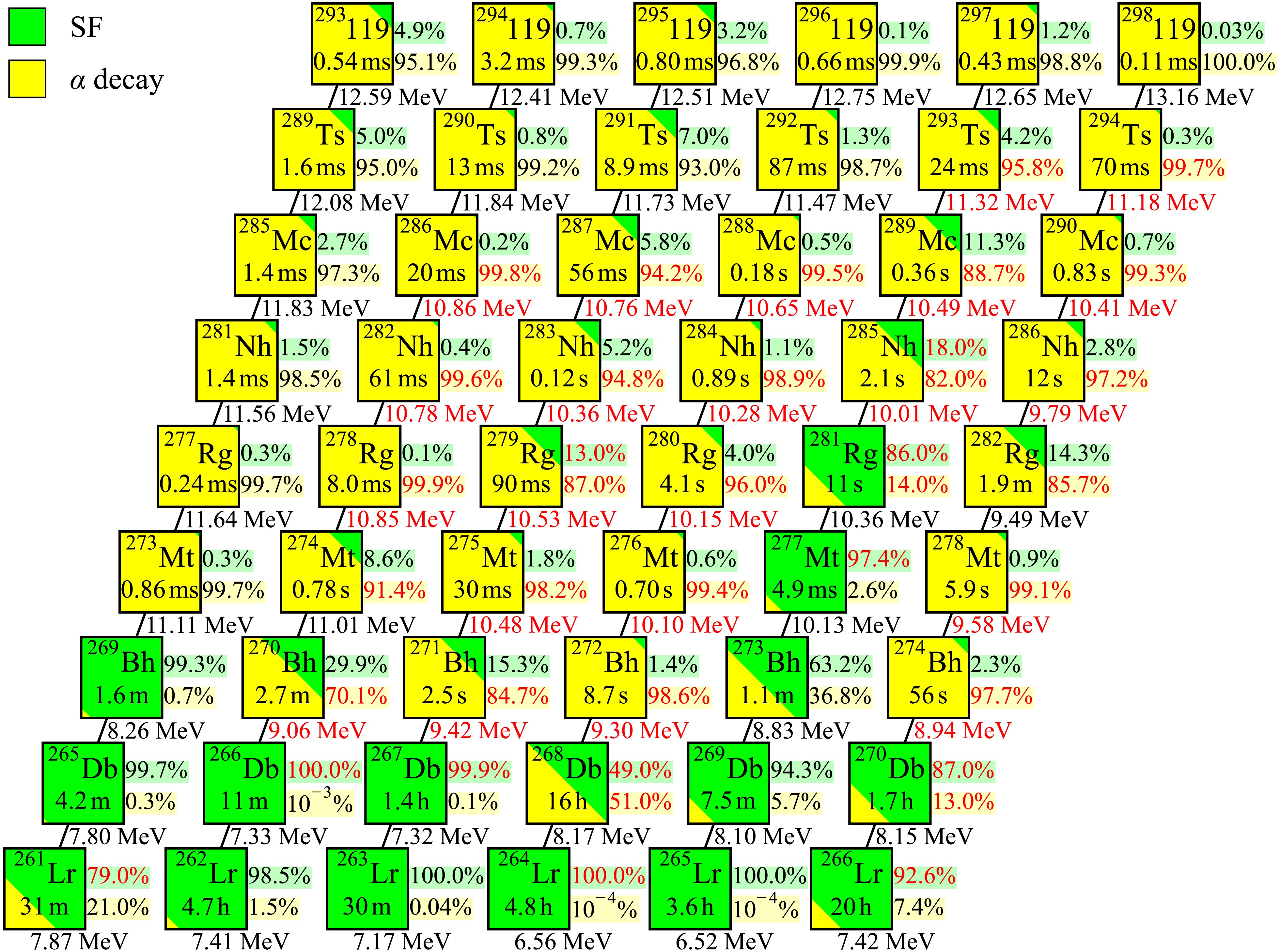

Figure 4.  (color online) $ \alpha $-decay chains of $ Z=119 $ isotopes with mass numbers A = 293–298. Each cell lists the nuclear symbol and the total half-life, taking into account competition between $ \alpha $ decay (yellow) and SF (green). The SF and $ \alpha $-decay branching ratios, $ b_{\rm{SF}} $ and $ b_{\alpha} $, respectively (in %), are given to the right of each cell ($ b_{\alpha}+b_{\rm{SF}} $ = 100%); the upper value is $ b_{\rm{SF}} $, and the lower value is $ b_{\alpha} $. Branching ratios shown in red indicate that the corresponding partial half-life was taken from experimental data [7, 10−13, 20, 29]; those shown in black indicate that the partial half-lives for $ \alpha $ decay and SF were calculated using Eq. (1) and Eq. (2), respectively. The $ Q_\alpha $ value for each parent nucleus is shown below the cell. Red $ Q_\alpha $ values are experimental [62], whereas black values are theoretical values obtained from Ref. [63].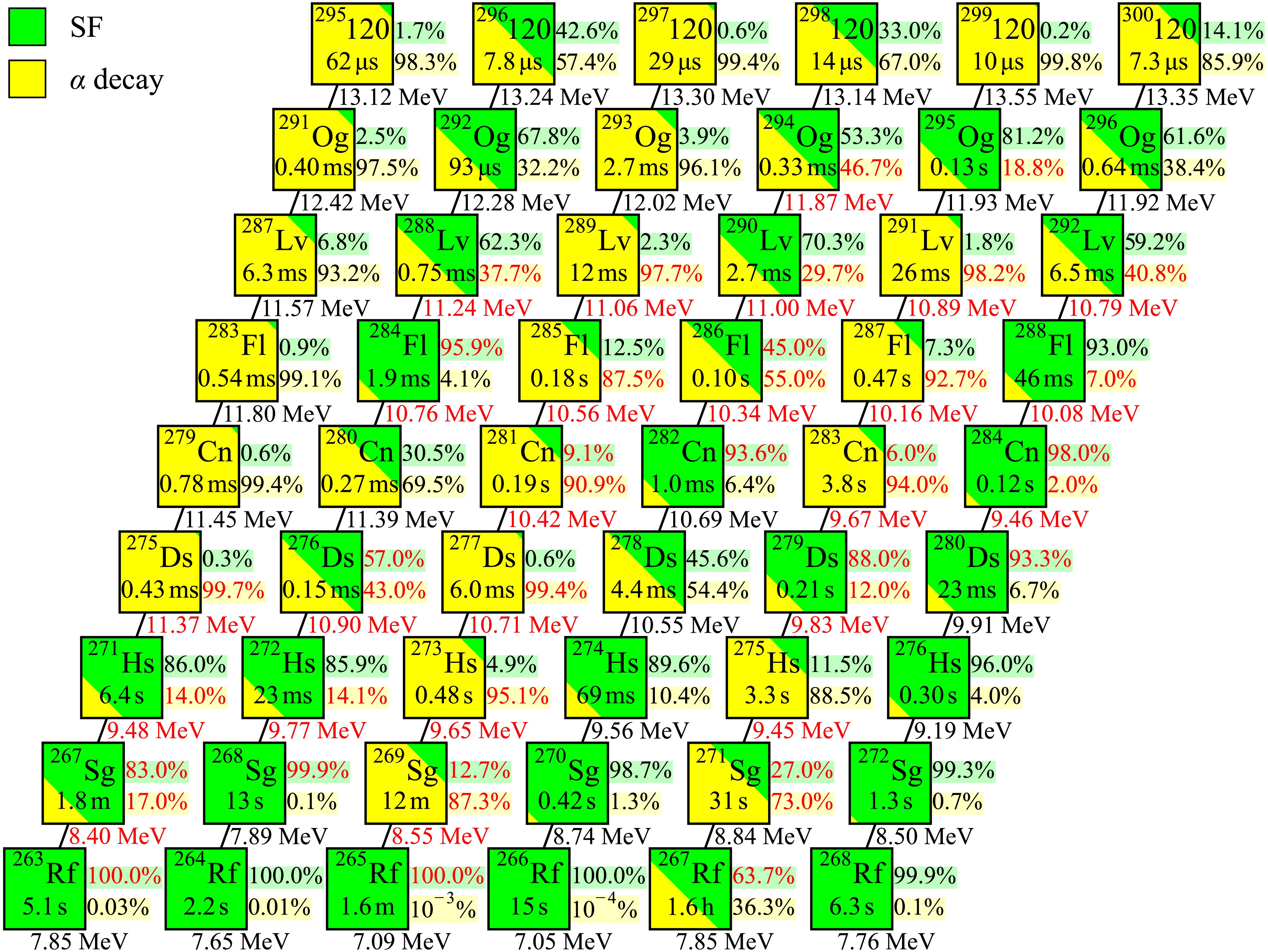

Figure 5.  (color online) Same as Fig. 4, but for the $ \alpha $-decay chains of $ Z=120 $ isotopes with mass numbers A = 295–300.

To systematically assess the competition between the two decay modes, we classify each nucleus according to the relative magnitudes of its partial half-lives. When the two half-lives differ by no more than one order of magnitude, i.e., $ \left| \log_{10} \left( T_{1/2}^{\alpha} / T_{1/2}^{\rm{SF}} \right) \right| \le 1 $, the nucleus is regarded as exhibiting strong competition between the two decay modes. Otherwise, if $ T_{1/2}^{\alpha} \lt T_{1/2}^{\rm{SF}} $, $ \alpha $ decay is considered to be the dominant mode, whereas if $ T_{1/2}^{\alpha} \gt T_{1/2}^{\rm{SF}} $, SF is considered dominant.

We now discuss each chain individually, focusing on the competition between $ \alpha $ decay and SF and on the prospects for experimental observation of the isotopes of elements 119 and 120 through their $ \alpha $-decay chains.

The most favorable cases for experimental identification are those in which $ \alpha $ decay remains the dominant mode over many consecutive steps, producing extended correlated sequences that terminate in SF. Among the isotopes of elements 119 and 120 considered here, this behavior is found in the chains starting from ^293,294,296119 and ²⁹⁵120. Here and below, the number of $ \alpha $ decays in a chain is defined as the number of consecutive $ \alpha $-emitting steps up to the first nucleus that undergoes SF.

Chain starting from ²⁹³119 ($ N-Z = 55 $). This chain provides six consecutive $ \alpha $ decays, from ²⁹³119 down to ²⁷³Mt. Throughout this sequence, $ \alpha $ decay remains clearly dominant. The transition to SF dominance occurs at ²⁶⁹Bh, where the chain terminates. The half-lives along the $ \alpha $-dominated part of the chain are in the submillisecond-to-millisecond range. This chain is among the most promising candidates for experimental identification.

Chain starting from ²⁹⁴119 ($ N-Z = 56 $). This chain yields seven $ \alpha $ decays, from ²⁹⁴119 down to ²⁷⁰Bh. The dominance of $ \alpha $ decay is clear from ²⁹⁴119 through ²⁷⁴Mt. At ²⁷⁰Bh, competition between the two modes becomes apparent, although $ \alpha $ decay still dominates. SF becomes dominant at ²⁶⁶Db. Our predictions for the nuclei from ²⁸⁶Mc onward are consistent with experimental data, which show only $ \alpha $ decays down to ²⁶⁶Db.

Chain starting from ²⁹⁶119 ($ N-Z = 58 $). This chain provides seven $ \alpha $ decays before SF terminates the sequence at ²⁶⁴Lr. The dominance of $ \alpha $ decay is clear from ²⁹⁶119 through ²⁷²Bh. At ²⁶⁸Db, our calculations predict strong competition between the two modes, and the experimental data confirm this competition.

Chain starting from ²⁹⁵120 ($ N-Z = 55 $). This chain provides six consecutive $ \alpha $ decays, from ²⁹⁵120 down to ²⁷¹Hs. Throughout this sequence, $ \alpha $ decay remains clearly dominant. At ²⁶⁷Sg, competition between the two modes emerges, and the chain terminates at ²⁶³Rf. Our predictions for the lower part of the chain are consistent with experimental data.

The chains discussed in this section contain one or more nuclei exhibiting strong competition according to the above criterion, although smaller but non-negligible SF branches may occur at other steps. Although these chains may still be observable as $ \alpha $ emitters, the presence of SF branches could affect the decay pattern or shorten the observed sequence in some cases. Such behavior is found in the chains starting from ^295,297,298119 and ^297,299120.

Chain starting from ²⁹⁵119 ($ N-Z = 57 $). The dominant decay sequence contains seven consecutive $ \alpha $ decay steps, from ²⁹⁵119 down to ²⁷¹Bh. A noticeable SF admixture appears at ²⁸³Nh and remains appreciable at ²⁷⁹Rg. For ²⁸⁷Mc, the experimental $ \alpha $-decay half-life is significantly shorter than our prediction, although $ \alpha $ decay remains the observed mode. The chain can terminate by SF at ²⁶⁷Db.

Chain starting from ²⁹⁷119 ($ N-Z = 59 $). This chain exhibits competition between $ \alpha $ decay and SF from the initial steps. A notable discrepancy with experiment appears at ²⁸¹Rg: while our calculations predict $ \alpha $-decay dominance with a significant SF admixture, the experimental data indicate SF as the dominant mode. An even larger discrepancy is observed at ²⁷⁷Mt, where the experimental SF half-life is three orders of magnitude shorter than our prediction. The chain terminates at ²⁶⁵Lr in our calculations, although the experimental observation of SF only for ²⁷⁷Mt indicates a possible earlier termination.

Chain starting from ²⁹⁸119 ($ N-Z = 60 $). Starting from ²⁹⁸119, the chain proceeds through seven consecutive $ \alpha $ decays down to ²⁷⁴Bh. A noticeable SF admixture appears at ²⁸²Rg and becomes strong at ²⁷⁰Db, where the two decay modes compete. Experimental data for ²⁷⁰Db indicate SF dominance, consistent with our predictions. The chain can terminate at ²⁶⁶Lr.

Chain starting from ²⁹⁷120 ($ N-Z = 57 $). The chain beginning at ²⁹⁷120 undergoes seven consecutive $ \alpha $ decays down to ²⁷³Hs before SF terminates the sequence at ²⁶⁹Sg. The dominance of $ \alpha $ decay is clear in the initial steps. Competition becomes noticeable starting from ²⁸⁵Fl and persists through ²⁷³Hs, apart from a return to $ \alpha $-decay dominance at ²⁷⁷Ds. At ²⁶⁹Sg, our calculations predict competition between the two modes, whereas only $ \alpha $ decay has been observed experimentally, indicating a possible overestimation of the SF branch in this nucleus.

Chain starting from ²⁹⁹120 ($ N-Z = 59 $). Among the $ Z=120 $ isotopes, the chain starting from ²⁹⁹120 is the longest $ \alpha $-dominated chain, with seven consecutive $ \alpha $ decays. Strong competition appears already at the second decay step, at ²⁹⁵Og, and persists throughout the chain. Notably, at ²⁷⁹Ds, our calculations predict $ \alpha $-decay dominance, whereas experimental data indicate strong competition with SF. The chain continues beyond ²⁶⁷Rf in our calculations, although the calculated SF branch becomes increasingly important.

For some isotopes, SF becomes the dominant decay mode at an early stage in the chain, preventing the observation of extended $ \alpha $-decay sequences. Among the isotopes of element 120, this behavior is found in the chains starting from ^296,298,300120.

Chain starting from ²⁹⁶120 ($ N-Z = 56 $). This chain exhibits strong competition between $ \alpha $ decay and SF from the first step, beginning with ²⁹⁶120, and this competition persists throughout the chain. For ²⁷⁶Ds, the experimentally observed competition between the two modes is consistent with our predictions. At ²⁷²Hs, however, only $ \alpha $ decay has been observed experimentally, whereas our calculations indicate a significant SF component. The chain terminates by SF at ²⁶⁸Sg, in agreement with experiment.

Chain starting from ²⁹⁸120 ($ N-Z = 58 $). This chain is characterized by strong competition already at ²⁹⁸120, and the two modes remain competitive throughout most of the chain. For ²⁹⁴Og and ²⁹⁰Lv, only $ \alpha $ decay has been observed experimentally, whereas our calculations predict competition with SF. For ²⁸⁶Fl, the experimental data confirm competition between the two decay modes.

Chain starting from ³⁰⁰120 ($ N-Z = 60 $). In this chain, strong competition is already present at ³⁰⁰120 and continues through ²⁹⁶Og and beyond. For ²⁹²Lv and ²⁸⁸Fl, only $ \alpha $ decay has been observed experimentally, whereas our calculations indicate strong competition with SF. For ²⁸⁴Cn, both the experimental data and our predictions show SF dominance, with both decay modes observed. At ²⁸⁰Ds, only SF has been observed experimentally, consistent with our calculated SF dominance. The early onset and persistence of strong competition with SF make this chain particularly unfavorable for experimental identification via $ \alpha $-decay chains.

The competition between $ \alpha $ decay and SF was analyzed along the $ \alpha $-decay chains of the as-yet-unsynthesized elements $ Z=119 $ and $ Z=120 $ in the mass ranges A = 293–298 and A = 295–300, respectively. These ranges correspond to neutron-excess values of $ N-Z $ = 55–60, which may be accessible in fusion-evaporation reactions. The $ \alpha $-decay half-lives were calculated using the Viola–Seaborg formula [45] with the Parkhomenko–Sobiczewski parameterization [56], whereas the SF half-lives were obtained using our recently proposed empirical formula [58, 59]. Theoretical $ Q_\alpha $ values were taken from the macroscopic–microscopic model of Ref. [63] when experimental values from Ref. [62] were unavailable.

The chains originating from ^293,294,296119 and ²⁹⁵120 are found to be the most favorable for experimental identification, with six or more consecutive $ \alpha $ decays expected. For the chains originating from ^295,297,298119 and ^297,299120, the presence of significant SF branches indicates a more complex decay pattern. Among the considered isotopes, the chains originating from ^296,298,300120 are the least favorable, with SF becoming dominant at early stages.

The present results may be of interest for ongoing experimental searches at JINR (Dubna) [8, 85, 86], LBNL (Berkeley) [87], GSI (Darmstadt) [23, 28, 88], RIKEN (Tokyo) [89], and IMP (Lanzhou) [90], all of which are currently pursuing the synthesis of elements 119 and 120 at the upper end of the nuclear chart.

Table 1 compares the calculated and experimental half-lives of 66 nuclei in the region $ 103 \le Z \le 118 $ and $ 55 \le N-Z \le 60 $ for which experimental data or limits are available for at least one decay mode. The total half-lives and branching ratios are obtained using Eq. (3) within the two-channel ($ \alpha $ decay + SF) approximation.

Table 2 presents the calculated $ \alpha $-decay and SF half-lives, the resulting dominant decay modes for the three considered input $ Q_\alpha $ values, and an indication of whether the predicted mode is robust against the $ Q_\alpha $ uncertainty.